the impact of different completion parameters on well … · well performance of gas unconventional...

The Impact of Different Completion Parameters on Well

Performance of Gas Unconventional Reservoirs

Ibrahim S. Mohamed, Hamid M. Khattab, Ahmed A. Gawish and Mazher H. Ibrahim

Abstract— Unconventional reservoirs are defined as reservoirs that cannot be produced at economic flow rates or that do not produce

economic volumes of oil and gas without assistance from massive stimulation treatments or special recovery process. Shale and tight

reservoirs are low quality reservoirs with low permeability. This low permeability can be as low as 100 Nano decries. . Well performance in

gas unconventional reservoirs is greatly affected by different completion parameters of the horizontal wells. These completion parameters

include number of frac stages, frac face skin, production under different draw down or (𝑝𝑖 - 𝑝𝑤𝑓) and the effect of production from

different drainage areas. In this study, these parameters will be studied and quantified for proper analysis of long-term linear flow periods

associated with tight/shale gas production.

Index Terms— Unconventional reservoirs, low permeability, . Well performance, , frac face skin, tight/shale gas, hydraulic fracture , completion configurations, draw down

—————————— ——————————

1. Introduction

Horizontal drilling and multistage hydraulic fracture are

the two key enabling technologies for the economic

development of ultralow permeability reservoirs as tight and

shale gas reservoirs (permeability in Nano Darcy).The use of

multi-fractured horizontal wells is expected to create a

complex sequence of flow regimes.

Well performance of gas unconventional reservoirs is greatly

affected by the different completion configurations between

the reservoir and the horizontal well. Completion parameters

that greatly affect the well performance include the number of

frac stages, frac face skin, production under different draw

down or (𝑝𝑖 - 𝑝𝑤𝑓) and the effect of production from different

drainage areas. These parameters should be studied and

quantified for proper analysis of long-term linear flow

periods associated with tight/shale gas production.

2. Methodology

GASSIM simulator is used, GASSIM is a single phase, 2D

simulator that is originally developed to simulate real gas

flow in both x-y and r-z domain. Later, it was modified to

include the ability to simulate liquid case. It is written in

Visual Basic code for Excel. It has been used extensively in

previous studies and proved to give accurate solutions.

3. The effect of number of the frac stages .

The effect of the number of stages of the hydraulic fractures

on well performance of gas unconventional reservoirs can be

studied in terms of the frac spacing.

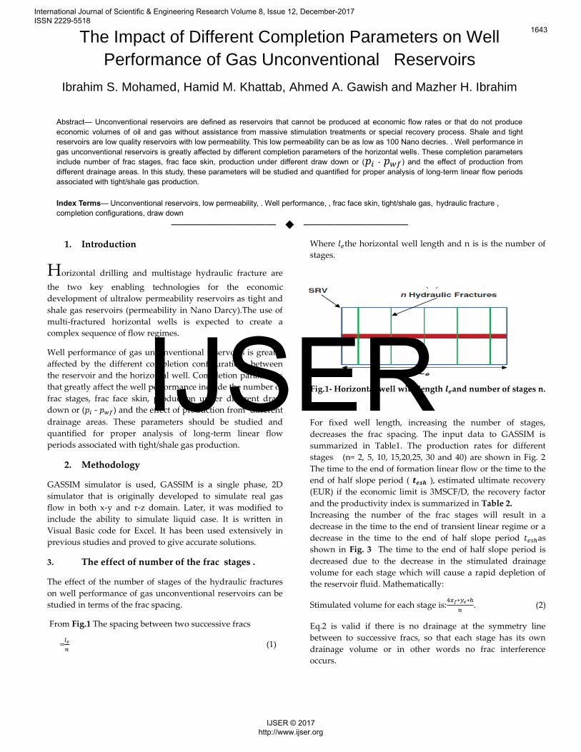
From Fig.1 The spacing between two successive fracs

=

(1)

Where the horizontal well length and n is is the number of

stages.

Fig.1- Horizontal well with length and number of stages n.

For fixed well length, increasing the number of stages,

decreases the frac spacing. The input data to GASSIM is

summarized in Table1. The production rates for different

stages (n= 2, 5, 10, 15,20,25, 30 and 40) are shown in Fig. 2

The time to the end of formation linear flow or the time to the

end of half slope period ( ), estimated ultimate recovery

(EUR) if the economic limit is 3MSCF/D, the recovery factor

and the productivity index is summarized in Table 2.

Increasing the number of the frac stages will result in a

decrease in the time to the end of transient linear regime or a

decrease in the time to the end of half slope period as

shown in Fig. 3 The time to the end of half slope period is

decreased due to the decrease in the stimulated drainage

volume for each stage which will cause a rapid depletion of

the reservoir fluid. Mathematically:

Stimulated volume for each stage is:

. (2)

Eq.2 is valid if there is no drainage at the symmetry line

between to successive fracs, so that each stage has its own

drainage volume or in other words no frac interference

occurs.

International Journal of Scientific & Engineering Research Volume 8, Issue 12, December-2017 ISSN 2229-5518

1643

IJSER © 2017 http://www.ijser.org

IJSER

Increasing the number of stages also decrease the total time

needed to deplete the reservoir due to increasing the

production rate as shown in Fig.4 Mathematically:

The total production of the total stages

= n* production of single stage (3)

Eq.3 is valid if we assume that all stages are identically and

equally spaced.

Although the initial rate increases with increasing the number

of stages ,the ratio of the initial rate to the rate at the

beginning the boundary dominated flow decreases which

indicates that the decline rate is higher when more stages are

added as shown in Fig. 5.

Increasing the number of stages also results in an increase in

the productivity index (PI).The increase in the productivity

index is a result of the increase in the production rate with

increasing the number of stages under constant bottom hole

flowing pressure i.e. constant 𝑝𝑤𝑓as shown in Fig. 6.

Table 1- The input data to GASSIM to simulate the effect of

changing the number of stages on well performance.

Fig. 2- The production rate for different stages on the same

graph .

Table 2- Summary of , EUR, total time, RF and PI for

different values of n.

Fig. 3-The effect of increasing frac stages on the transient

linear period.

Fig. 4-The effect of inceasing frac stages on the total

depletion time till economic limit is reached .


1644


IJSER

Fig. 5-The ratio between the initial rate to the rate at the

beginning of the boundary dominated flow.

Fig. 6-The effect of increasing frac stages on the productivity

index.

Increasing the number of stages, increases the

cumulative production as shown in Fig. 7 and Fig. 4.8 . Fig.

4.9 is the percentage of production increase for n> 2 and n>15

after 14000 day of production . As shown in Fig.4.9, increasing

the number of stages from n=2 to n=5,10,15 will result in a

percentage of production increase of 60%, 73.6%, 75.5%

while increasing the number of stages from n=2 to n=40

results in a percentage of production increased of

77%.Increasing the number of stages from n=15 to n=40 results

in percentage of production increase of 5%. Similar results

after 2000 day of production is shown in Fig.4.10 .

The number of stages should be economically optimum and

determined in terms of the in situe conditions of the reservoir

, the estimated ultimate recovery and the expected production

period. Fig. 11 is the percentage of production increase if the

production period extended from 2000 to 14000 day .As

shown from Fig.11 that for n=2,5,10,15 extending the

production period from 2000 to 14000 will result in a

percentage of production increase of 60% ,58%,48%,35%while

for n= 40 increasing the production period will result in

average production increase of 3.8% .

Fig. 7–The cumulative production with the time for

different stages.

Fig. 8– The cumulative production different stages after

14000 day.

Fig. 9- The percentage of production increase for n> 2 and

n>15 after 14000 day of production.


1645


IJSER

Fig. 10- The percentage of production increase for n> 2 and

n>15 after 2000 day of production.

The number of stages should be economically optimum and

determined in terms of the in situe conditions of the reservoir

, the estimated ultimate recovery and the expected production

period. Fig. 11 is the percentage of production increase if the

production period extended from 2000 to 14000 day .As

shown from Fig.11 that for n=2,5,10,15 extending the

production period from 2000 to 14000 will result in a

percentage of production increase of 60% ,58%,48%,35%while

for n= 40 increasing the production period will result in

average production increase of 3.8% .

Fig. 11- Percentage of production increase if the production

period extended from 2000 to 14000 day.

4. Effect of fracture face skin.

Fracture face skin is modeled in two different models as

chocked fracture damage and fracture face damage

Chocked fracture damage occurs when the region around the

well bore has a reduced permeability. Choked fracture

damage originates when the proppant within the fracture is

embedded or crushed or lost as shown in Fig.12 Where

, , are the chocked fracture length , the permeability of

the damaged zone and the width of the damaged zone

respectively. Fracture face damage occurs due to the filtration

of the fracturing fluid into the formation and formation of

filter cake. Filtration and filter cake reduce the permeability in

the region surrounding the frac as shown in Fig.4.13 .

Different values of fracture face skin (0, 0.01, 0.02, 0.05, 0.07,

0.1, 0.2, 0.5, 0.7, 1) are used to study the impact of skin on the

well performance. The data used for simulation is

summarized in Table 3. As the fracture face skin increases, the

linear flow regimes dimensioned gradually and look like

another flow regimes. This is could lead to wrong analysis for

the well performance and reservoir parameters estimated

from wrong flow regime as shown in Fig. 14.

Fig. 12- Choked fracture damage from

.

Fig. 13- Hydraulic fracture with fracture face damage

from .

For small values of frac face skin i.e ( 𝑓𝑓=0.0. 𝑓𝑓=0.01, 𝑓𝑓=0.05,

𝑓𝑓=0.1), the linear flow regime or half slope on log- log plot is

changed at early time and the curves become more flatten but

finally linear flow is reached or the half slope appears .The

flatness of the curves may cause misinterpretation of the well

performance during the early production period. The flat part

of the curve indicates a transient radial flow which is

completely incorrect. Other note is that, although the small

values of skin change the shape of the production rate on the

log-log plot, the total production time is nearly the same i.e.

the curves are matched. For large values of skin ( 𝑓𝑓=0.5

, 𝑓𝑓=1), the linear flow regime doesn't appear on the log –log

plot at all but complete transient radial and boundary flow

appear on the log-log plot and the total production time

increased


1646


IJSER

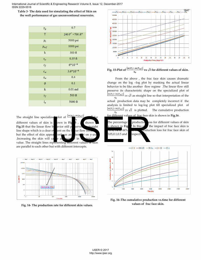
Table 3- The data used for simulating the effect of Skin on

the well performance of gas unconventional reservoirs.

The straight line specialized plot of [ ]

vs √ for

different values of skin is shown in Fig.15 . As shown in

Fig.15 that the linear flow behavior still preserves its straight

line shape which is a clear evident on the linear flow behavior

but the effect of skin appears only as an intercept on y-axis

.Increasing the skin will cause an increase in the intercept

value. The straight lines representing different values of skin

are parallel to each other but with different intercepts.

Fig. 14- The production rate for different skin values.

Fig. 15-Plot of [ ]

vs √ for different values of skin.

From the above , the frac face skin causes dramatic

change on the log –log plot by masking the actual linear

behavior to be like another flow regime .The linear flow still

preserve its characteristic shape on the specialized plot of [ ]

vs √ as straight line so that interpretation of the

actual production data may be completely incorrect if the

analysis is limited to log-log plot till specialized plot of [ ]

vs √ is plotted. The cumulative production

for different values of frac face skin is shown in Fig.16 .

The percentage of production loss for different values of skin

is shown in Fig.17 In this case the impact of frac face skin is

7.6%, 14%, 44% and 60% production loss for frac face skin of

0.05,0.1,0.5 and 1, respectively.

Fig. 16–The cumulative production vs.time for different

values of frac face skin.


1647


IJSER

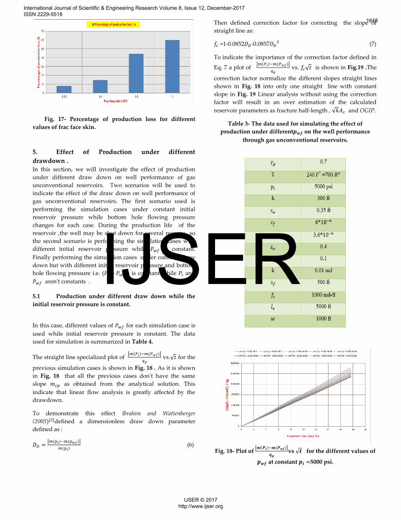
Fig. 17- Percentage of production loss for different

values of frac face skin.

5. Effect of Production under different

drawdown . In this section, we will investigate the effect of production

under different draw down on well performance of gas

unconventional reservoirs. Two scenarios will be used to

indicate the effect of the draw down on well performance of

gas unconventional reservoirs. The first scenario used is

performing the simulation cases under constant initial

reservoir pressure while bottom hole flowing pressure

changes for each case. During the production life of the

reservoir ,the well may be shut down for several reasons so

the second scenario is performing the simulation cases with

different initial reservoir pressure while 𝑤𝑓 is constant.

Finally performing the simulation cases under constant draw

down but with different initial reservoir pressure and bottom

hole flowing pressure i.e. ( 𝑖 𝑤𝑓 ) is constant while 𝑖 and

𝑤𝑓 aren't constants .

5.1 Production under different draw down while the

initial reservoir pressure is constant.

In this case, different values of 𝑤𝑓 for each simulation case is

used while initial reservoir pressure is constant. The data

used for simulation is summarized in Table 4.

The straight line specialized plot of [ ]

vs.√ for the

previous simulation cases is shown in Fig. 18 . As it is shown

in Fig. 18 that all the previous cases don't have the same

slope as obtained from the analytical solution. This

indicate that linear flow analysis is greatly affected by the

drawdown.

To demonstrate this effect Ibrahim and Wattenberger

(2005 defined a dimensionless draw down parameter

defined as :

[ ]

(6)

Then defined correction factor for correcting the slope of

straight line as:

=1-0.0852 -0.0857 (7)

To indicate the importance of the correction factor defined in

Eq. 7 a plot of [ ]

vs. √ is shown in Fig.19 .The

correction factor normalize the different slopes straight lines

shown in Fig. 18 into only one straight line with constant

slope in Fig. 19 Linear analysis without using the correction

factor will result in an over estimation of the calculated

reservoir parameters as fracture half-length , √ and OGIP.

Table 3- The data used for simulating the effect of

production under different on the well performance

through gas unconventional reservoirs.

Fig. 18- Plot of [ ]

vs √ for the different values of

at constant 5000 psi.


1648


IJSER

Fig. 19- [ ]

vs √ for the different values of

at constant 5000 psi.

5.2 Production under constant while the initial

reservoir pressure isn't constant .

Different scenario to indicate the effect of production under

different draw down while the initial reservoir pressure is not

constant but 𝑝𝑤𝑓 is constant. During the production period

the well may be shut for different reasons but when the

production is continued the reservoir pressure may be not at

the initial reservoir pressure during the initial production

period. To show the effect of production under different

initial reservoir pressure different simulation cases are run

with constant 𝑝𝑤𝑓. The input data used to run these

simulation cases is the same data in Table 4 but with

𝑝𝑤𝑓=2000 psi and 𝑝𝑖=6000,5000,4000,3000 and 2500 psi.

A plot of [ ]

vs. √ is shown in Fig. 20. As shown in

Fig. 20 that different straight lines with different slopes is

obtained for different 𝑝𝑖.The reason for these different slopes

straight lines is the reservoir and fluid pressure dependent

properities √( )𝑖 . To obtain a single straight line with

constant slope it is preffered to plot [ ]

𝑓

√( )

√ or √( )𝑖

[ ]

√

to eleminate the effect of the pressure dependent properities

and obtaining a single straight line with constant slope as

shown in Fig.21.

6. The effect of Production from different

drainage area on well performance In this section we will study the effect of production from

different drainage areas on well performance of gas

unconventional reservoirs . This effect will be studied by

assuming that the horizontal well isn’t completely penetrate

the reservoir .Assuming different horizontal well lengthes (

with constant number of stages.In the previous study of the

impact of different fracture stages we assumed a constant

Fig. 4. 20-Plot of

vs √ for the different values

of at constant 2000 psi.

The slope of the straight line in Fig.4.31 is

√

which is constant for the same reservoir because it doesn't

include any pressure dependent properties. This slope can be

used for the straight line analysis to obtain the different

reservoir and frac properties.

Fig. 21-Plot of √( )

[ ]

√ for the

different values of at constant 2000 psi.

reservoir length but the number of stages was variable. The

data used for simulationg the effect of different drainage

areas is summerised in Table 5.The well length is changed in

each simulation case ( =1000, 2000, 3000, 4000 and 5000 ft).

The effect of different drainage areas or frac spacing on the

well performance can be illustrated by plotting all the

previous cases on the same log log plot as shown in Fig. 22.


1649


IJSER

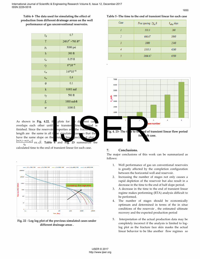
Table 4- The data used for simulating the effect of

production from different on the well

performance of gas unconventional reservoirs.

As shown in Fig. 4.22, the plots for the different cases

overlaps each other until the transient linear period is

finished. Since the reservoir properties and the fracture half-

length are the same in all these simulated cases so that they

have the same slope on the straight line specialized plot of [ ]

√ . Table 6 and Fig. 23 summarize the

calculated time to the end of transient linear for each case.

.

Fig. 22 - Log log plot of the previous simulated cases under

different drainage areas .

Table 5 -The time to the end of transient linear for each case

.

Fig. 4. 23- The time to the end of transient linear flow period

for each case.

7. Conclusions. The major conclusions of this work can be summarized as

follows:

1. Well performance of gas un conventional reservoirs

is greatly affected by the completion configuration

between the horizontal well and reservoir.

2. Increasing the number of stages not only causes a

rapid depletion of the reservoir but also result in a

decrease in the time to the end of half slope period.

3. A decrease in the time to the end of transient linear

regime makes performing (RTA) analysis difficult to

be performed.

4. The number of stages should be economically

optimum and determined in terms of the in situe

conditions of the reservoir , the estimated ultimate

recovery and the expected production period

5. Interpretation of the actual production data may be

completely incorrect if the analysis is limited to log-

log plot as the fracture face skin masks the actual

linear behavior to be like another flow regimes so


1650


IJSER

the straight line specialized plot is required for

proper interpretation as the skin appears only as an

intercept on y-axis .

6. RTA is a draw down dependent analysis so that

performing RTA without the use of the correction

factor developed by Ibrahim and wattenberger would

result in over estimation of the reservoir properties.

7. The length of the horizontal well throught out the

reservoir only results in an increase in the time of the

end of transient linear flow but has no effect on the

straight line specialized plot .

8. NOMENCLATURE = half width of the reservoir, ft

𝑓= frac half length ft

= half distance between two successive fracs ,ft

𝑝𝑤 = dimensionless pressure

= dimensionless time based on half width of the reservoir

=dimensionless time based on half distance between two

successive fracs

= dimensionless rate

𝑤 = dimensionless pseudo pressure

𝑝𝑖 = pseudopressure at initial reservoir pressure,

𝑝𝑤𝑓 pseudopressure at bottom hole flowing pressure

,

= gas flow rate, MSCF/D

= reservoir tempreture, ,

= reservoir permeability , md

= total compressibility,

= gas viscosity, cp

= porosity

=slope in case of constant rate

=slope in case of constant pressure

= reservoir thickness , ft

= cross sectional area to the flow,

= time to the end of half slope period ,Day

= pore volume

= original gas in place,BSCF.

𝑖 = gas formation volume factor at initial reservoir pressure

,RB/STB

= reservoir extension, ft

9. REFERENCES (1) Cinco-Ley, H., Samaniego-V., F. 1981. Transient

Pressure Analysis: Finite Conductivity Fracture

Case Versus Damaged Fracture Case. Paper SPE

10179 presented at the SPE Annual Technical

Conference and Exhibition, San Antonio, Texas,

USA, 4–7 October.

(2) Ibrahim, M. and Wattenbarger R.A. 2005. Rate

Dependence of Transient Linear Flow inTight

Gas Wells. Paper CIPC 2005-057 presented at

Canadian International

Petroleum Conference, Calgary, Alberta, 7–9

June. DOI: 10.2118/2005-057.


1651


IJSER

the impact of different completion parameters on well … · well performance of gas unconventional...

Documents