The Impact of Economic Shocks on Wage Dynamics in Indonesia

Lukas Hensel∗

January 12, 2017

Abstract

This paper tests for downward nominal wage rigidity in agricultural labour markets using transitory

labour demand shocks induced by plausibly exogenous rainfall fluctuations. The results suggest that

downward adjustment of nominal wages is a function of the cost of maintaining the nominal wage at

the prevailing level: nominal wages adjust downwards when these costs are high, while they remain

fixed when the costs of keeping the wage level constant are relatively low. In particular, I exploit the

fact that past positive productivity shocks exogenously increase these costs by raising the prevailing

nominal wage level. I show that nominal wages only decline when negative productivity shocks are

preceded by a positive shock. By providing convergent evidence from large repeated cross-sections

and data on individual nominal wage changes, I rule out that my results are driven by composi-

tional changes in my sample or selective migration. Furthermore, I provide evidence of persistent

employment effects of positive agricultural productivity shocks, which suggests that the potential

negative employment effects of downwardly rigid nominal wages can be at least partially offset by

employment rigidities. I present a simple model of agricultural labour markets including reference

dependent utility over nominal wage cuts and firing frictions which is consistent with the observed

wage and employment rigidities.

JEL Codes: J23, J31, J43, Q12

∗St. Peter’s College, University of Oxford, New Inn Hall St, OX1 2DL Oxford, lukas.hensel@economics.ox.ac.uk. I am

grateful to my supervisor Dr. Climent Quintana-Domeque for his guidance and encouragement in working on this paper.

I also thank Christopher Roth for valuable feedback throughout the process of writing this paper. For helpful discussions

and feedback, I thank Simon Franklin, Douglas Gollin, Surpreet Kaur, Clement Imbert, Simon Quinn, Jan Priebe, Giulio

Schinaia, Timo Reinelt, Sasha Parameswaran, and my wonderful girlfriend Sangjung Ha. I gratefully acknowledge financial

support by the German National Academic Foundation and the German National Academic Exchange Service.

1

1 Introduction

Labour market frictions can have important economic consequences. This is particularly true for de-

veloping countries, where labour typically comprises a larger share of factor inputs for production.

Well-functioning labour markets in developing countries are important to mitigate the impact of eco-

nomic shocks (Colmer, 2015) and for efficient allocation of labour resources (Bryan and Morten, 2015).

The wage - as the price of labour - plays a particularly important role in the functioning of labour mar-

kets: partial or non-adjustment of wages to economic shocks can have vital consequences for profits,

employment and production. In particular, downward rigidity of nominal wages is a potential source of

large economic distortions, which may result in the misallocation of factor inputs. A long literature has

examined the economic effects of downward nominal wage rigidity, ranging from employment effects

(Card, 1990; Altonji and Devereux, 2000; Kaur, 2015) to aggravated business cycle volatility (Clarida

et al., 1999; Galı, 2009; Benigno and Ricci, 2011).

A large body of literature has described the existence of downward nominal wage rigidity in developed

countries (Akerlof et al., 1996; Dickens et al., 2007). However, the results of recent empirical work using

credible identification strategies to test for downward nominal wage rigidity in developing countries is

contradictory. Kaur (2015) finds strong evidence of downward rigidity of nominal agricultural wages in

response to agricultural productivity shocks in India, whereas Franklin and Labonne (2016) find a large

degree of downward flexibility of nominal wages following a typhoon in the Philippines.1 This paper

contributes to the existing literature by leveraging both a large repeated cross-section and individual

level wage change data from Indonesia to analyse the determinants of downward nominal wage rigidity

in agricultural labour markets in Indonesia.

I show that agricultural wages in Indonesia are at least partially downwardly flexible and provide

evidence that treating downward nominal wage rigidity as binary is an oversimplification. To explain

the heterogeneous adjustment patterns of nominal wages to economic shocks, I introduce the effective

productivity gap that measures the cost of not adjusting the wage downwards. In particular, I exploit

differences in the prevailing nominal wage induced by past productivity shocks to show that wages only

adjust downwards for large values of the effective productivity gap.

1The different findings of these papers could potentially be explained by several factors: Kaur (2015) relies on cross-sectional and district level data, whereas Franklin and Labonne (2016) use high frequency panel data. The different natureof the shocks analysed could also drive the diverging results. Both the duration and the specificity of shocks could influencewages: Typhoons are more permanent (i.e. they destroy capital) and less specific (i.e. they affect more than just theagricultural sector). The employment status of workers also varies between the two papers: Kaur (2015) uses wage databy agricultural day labourers and Franklin and Labonne (2016) find evidence for more flexibility with permanent workers.Also, if fairness norms determine downward rigidity of wages as suggested by Kaur (2015) different cultural contexts couldlead to divergent results.

2

The empirical analysis of downward nominal wage rigidity and its consequences faces several chal-

lenges. Studies using cross-sectional wage level data are generally subject to aggregation bias due to

endogenous sample composition (Bils, 1985; Keane et al., 1988; Keane and Prasad, 1996). The use of

wage change data allows to partially deal with this endogeneity, however it makes the analysis of aggre-

gate employment effects generally more difficult.2 Another common problem in many of the empirical

studies on downward rigidity of nominal wages is the difficulty of plausibly identifying exogenous shocks

to labour demand. This paper overcomes both of these problems. First, to identify exogenous and

transitory labour demand shocks, I follow Kaur (2015) and exploit the fact that rice yields, the main

agricultural crop in large parts of Indonesia, depend on monsoon rainfall (Naylor et al., 2007; Levine

and Yang, 2014). I validate my preferred rainfall measure by demonstrating that it predicts rice yields

in Indonesia over the sample period from 1993 to 2010. Second, I provide convergent evidence from

both large repeated cross-sections and individual-level wage change data. This allows me to plausibly

rule out that my results are driven by compositional changes or selective migration, while also enabling

me to analyse aggregate employment effects.

In contrast to much of the existing literature, I find that downward nominal wage rigidity does not

necessarily cause negative employment effects. I argue that the negative effects can be partially offset

by rigidities in the firing of workers. In particular, I provide evidence that the employment effects of

positive labour demand shocks are persistent and that the non-downward adjustment of nominal wages

to negative productivity shocks does not necessarily lead to a decrease in employment.

The findings of my analysis speak to a number of different literatures. First, I contribute to the

wider understanding of labour market reactions to weather-induced productivity shocks (Dell et al.,

2014, provide a comprehensive overview). The empirical results of this analysis reinforce the notion that

past weather events matter for current wage dynamics. Using a model of agricultural labour markets

I show that the effect of past positive shocks is theoretically ambiguous: past positive shocks could

lead current nominal wages to either increase or decrease. My results suggest that nominal wages

are partially downwardly flexibility, which is in line with a large part of the existing literature on wage

dynamics and economic shocks in developing countries. Jayachandran (2006), Franklin and Labonne

(2016), and Gignoux and Menendez (2015) all find some degree of elasticity of wages with respect to

negative economic shocks. On the other hand, my results contrast with Kaur (2015)’s finding of fully

downwardly rigid nominal wages and Kirchberger (2014)’s result of positive short term wage effects of

earthquakes.

2Card (1990) and Franklin and Labonne (2016) are rare exceptions.

3

Second, my paper also contributes to the literature on the efficiency of labour market reactions

to economic shocks. Flexible labour markets can be important mechanisms to mitigate the impact of

negative economic shocks, especially when those shocks are predictable (Rosenzweig and Udry, 2014;

Colmer, 2015; Groger and Zylberberg, 2016). On the other hand, factors hindering labour mobility or

job search can lead to large individual and aggregate economic inefficiencies (Bryan and Morten, 2015;

Franklin, 2015). My results show that wage and employment rigidities have the potential to partially

offset each other. Rigidities in the firing process in particular have the potential of mitigating the

negative employment effects of downward nominal wage rigidity.

Third, I provide a theoretical extension of Kaur (2015)’s model which explains downward nominal

wage rigidity using reference dependent utility of workers over nominal wage cuts: workers perceive a

nominal wage cut as unfair which leads them to reduce their effort. My contribution is to show that

these fairness norms only bind for certain intensities of productivity shocks and I show that nominal

wages can be downwardly flexible in equilibrium. I further augment the model with firing frictions to

explain persistent employment effects.

2 The Model

The theoretical analysis in this paper is based on Kaur (2015), but I extend her analysis by showing

that the model is also consistent with partially downwardly flexible nominal wages. The model describes

a agricultural labour markets in a static, small open economy with simultaneous wage setting and

exogenous producer prices.3 Workers exhibit reference dependent utility modelled as exogenous fairness

norms, which cause them to work with less effort if they are paid below their reference wage.4 My

contribution is to show that the cost of not adjusting the nominal wage downwards can be greater than

cost of accepting a lower effort induced by violated fairness norms.

3I briefly discuss implications of dynamic setting at the end of the section.4This specification is based on research suggesting that workers reduce effort in response to wage which are perceived

as unfair: Fehr et al. (2009) summarize the existing literature on fairness norms and labour markets and find that effortresponds particularly strongly to nominal wage cuts below a ’fair’ wage. Their review builds on theoretical models (Akerlofand Yellen, 1990), qualitative evidence (Bewley, 1995), and experimental findings (Fehr and Falk, 1999).

4

2.1 Set-up

There is a continuum of workers i with a mass normalized to one. I further normalize their payoff from

not working to zero. The utility function of worker i is:

Ui = u

(w

p

)− ψie

(1 +

1− λλ

1w<wt−1

)(1)

u(·) is a continuous, increasing, twice-differentiable, and concave function. w is the contemporaneous

nominal wage, p is the price level, and wt−1 is last period’s average nominal wage which is assumed

to be the reference wage.5 Note that I omit the t subscripts for contemporaneous variables due to the

static nature of the model. The reference wage is the only intertemporal component of the model.

1w<wt−1 is an indicator function, which is equal to one if the paid wage is below the reference wage.

The individual disutility of labour ψi indexes all workers and is uniformly distributed on [0, ψ]. e is the

level of effort workers exert, which is discontinuous around the reference wage:

e =

1, if w ≥ wt−1

λ, if w < wt−1

(2)

If workers are paid at least the reference wage, they exert effort e = 1. Workers reduce their effort to

λ ∈ (0, 1] if they are paid less than the reference wage. λ = 1 means that workers have no fairness

concerns. Note that workers decrease effort by exactly the amount needed to offset the disutility induced

by the violation of the fairness norm. Thus, the individual utility of accepting a wage offer w is

U(w) = u

(w

p

)− ψi (3)

This implies the following aggregate labour supply equation:

Ls =u(wp )

ψ(4)

There are J identical firms, where J is arbitrarily large. Firm j has the following profit function:

πj = pθf(Lje)− wjLj (5)

5Throughout this analysis I follow Kaur (2015) in focussing on pure strategy Nash Equilibria. This means that allworkers will be paid the same wage each period so that reference wage also equals worker i’s last period wage.

5

θ > 0 is the level of productivity, Lj is labour employed by firm j, Lje is effective labour, and wj

is the nominal wage set by firm j. f(·) is a continuous, increasing, twice differentiable, and concave

production function.

I assume that firms simultaneously set wages to maximize their profits. Furthermore, I assume that

firms hire labour in descending order of their wage offer. If multiple firms offer the same wage, the order

of hiring will be random between all firms offering the same wage. I further assume that workers with

the lowest disutility of labour will get hired first.6

2.2 Benchmark: Solution without Reference Dependence

If workers are paid strictly more than the reference wage or they do not exhibit fairness norms the level

of effort is constant at e = 1. If workers are paid strictly less than the reference wage and they exhibit

fairness concerns, the effort is constant at e = λ. Wage setting in either of those cases is not influenced

by the discontinuity in the effort introduced by fairness norms. Thus, at a given wage w∗ the first order

condition of the firm (6) determines individuals’ labour demand in either of those cases:

w∗(e, θ, p) = peθf ′(eL∗), for e ∈ {λ, 1} (6)

where I refer to w∗(e, θ, p) as the benchmark wage at effort level e.

Market clearing requires that labour demand equals labour supply:

JL∗ =u(wp )

ψ(7)

Proposition 1. Market clearing without reference dependence

For a constant level of worker effort e ∈ {λ, 1}, equations (6) and (7) determine labour supply and the

wage in the unique pure strategy Nash Equilibrium for all values of θ.

Proof. See Appendix A.1. �

Proposition 1 states that there is a unique pure strategy Nash Equilibrium in the benchmark case of

no fairness concerns (e = 1) and the case of permanently low effort (e = λ). It further states that

this equilibrium is fully described by the labour market clearing condition (7) and the firm’s first order

condition (6).

6As described by Kaur (2015), the specification of an allocation mechanism is necessary to prove the propositions.

6

2.3 The Impact of Fairness Concerns: Downward Rigidity

Fairness concerns introduce a discontinuity into to the firms’ profit function. To see this note that the

first order condition of the firms is discontinuous around last period’s average wage wt−1. In this case,

the first order condition for a given wage w is:

w =

pθf ′(L), if w ≥ wt−1

pθλf ′(λL), if w < wt−1

(8)

For w ≥ wt−1 the first order condition corresponds to the benchmark case of full effort e = 1. If

w < wt−1 the first order condition reflects the lower productivity of each unit of labour at the lower

level of effort, e = λ.

Let θR be implicitly defined as w∗(1, θR, p) = wt−1, i.e. the productivity level at which the reference

wage equals the market clearing wage at full effort. Further denote L∗(e, θ, p, w∗) as the labour demand

at w∗(e, θ, p). The labour demand at the reference wage (w = wt−1) is determined by the first

order condition (6) and is L(1, θ, p, wt−1).7 π∗(e, θ, w∗, L∗) and π(1, θ, wt−1, L) are the profits at the

respective wage levels. From here onwards, I only show the arguments of the function which are relevant

to the analysis.

Proposition 2. Asymmetric adjustment of wages to shocks

For λ sufficiently close to 1 there exists a 0 < θ′R < θR such that

1. For 0 < θ ≤ θ′R, all firms j setting wj = w∗(λ, θ, p) < wt−1 is a pure strategy Nash Equilibrium.

Furthermore, wj = wt−1 for all j is the only other candidate pure strategy Nash Equilibrium and∫ 10 π∗(λ, θ, w∗)dj >

∫ 10 π(1, θ, wt−1)dj.

2. For θ′R < θ ≤ θR all firms setting wj = wt−1 is the unique pure strategy Nash Equilibrium.

3. For θR < θ the wage will correspond to the benchmark case wj = w∗(1, θ, p).

Proof. See Appendix A.2. �

I extend Kaur (2015)’s model by distinguishing between three ranges of productivities. Proposition 2

states that as long as the decrease of workers’ effort in response to violated fairness norms is sufficiently

small, for low levels of productivity θ < θ′R firms would not deviate upwards from the benchmark wage

at low effort (w∗(λ, θ, p)) if all firms set this wage. It further states that total profits at the only other

candidate pure strategy Nash Equilibrium are smaller than at the aforementioned equilibrium. Thus,

7I will omit the reference to the effort from now on, as effort is always 1 at the reference wage.

7

while downward adjustment of wages is not necessarily the unique pure strategy Nash Equilibrium, it

can be argued that it is the only plausible equilibrium, as long as coordination costs are relatively low.8

At medium levels of productivity θ′R < θ ≤ θR, the only pure strategy Nash Equilibrium wage will be all

firms setting the reference wage and there will be excess labour supply. For high levels of productivity

(θ ≥ θR), the reference wage does not bind and wages will correspond to the benchmark case.

2.4 The Impact of Past Productivity

To facilitate the analysis of past shocks, Proposition 3 introduces the effective productivity gap denoted

by ρ. It is a measure of how costly it would be to maintain nominal wages at last period’s level. It

incorporates three factors which influence these costs: current productivity lowers the cost by increasing

the current benchmark nominal wage level; last period’s productivity increases the cost by raising last

period’s nominal wage level, and inflation decreases the cost by increasing current real wage levels. Note

that throughout this analysis I normalize the past price level pt−1 to one such that inflation is equivalent

to the contemporaneous price level p.

Proposition 3. The effective productivity gap

Define the effective productivity gap as ρ(θt, θt−1, p) = θt−1

θtp−1. Further define the reference wage

implicitly by wt−1 = θt−1f′(L) and equation (7). The following holds:

1. ρ ≤ 1⇔ θ ≥ θR, and there exists ρ∗ such that ρ∗ ≥ ρ > 1⇔ θ′R ≤ θ < θR.

2. An increase in θt−1 widens the range of θt for which wages adjust downwards.

Proof. See Appendix A.3. �

The advantage of using ρ is that one can directly analyse the impact of past shocks. Proposition

3 assumes that the last period’s wage was set according to the the benchmark case.9 Part one states

that there is a one-to-one mapping from ρ to θ such that ρ can be used to determine the predicted

wage level. The second part states that increases in past productivity make downward adjustment of

current nominal wages more likely, by increasing the cost of maintaining last period’s wage level. This

prediction is the main driver of the interpretation of my empirical results.

8In the context of Indonesian village labour markets, this is a reasonable assumption. While there are many potentialemployers in each village, there is a substantial amount of cooperation going on. According to the 1993 Indonesian VillageCensus (PODES) 60% of villages in districts included in this analysis have a farmers’ cooperative. In Java which is themost populous Island, this share goes up to 80%. This indicates a large amount of cooperation between farmers, whichsupports the assumption.

9I show empirically that considering further lags of productivity does not alter the results.

8

2.5 The Effect on Labour Supply

The model yields the following predictions for the employment relative to the benchmark case.

Proposition 4. The effect on labour supply

The following holds for total employed labour Le relative to labour employed in the benchmark case

L∗(1, w∗):

1. L∗(1, w∗) > Le = L(1, wt−1) if ρ ∈ (1, ρ∗)

2. L∗(1, w∗) = Le = L(1, wt−1) if ρ ≤ 1

3. The prediction for Le = L∗(λ,w∗(λ)) relative to L∗(1, w∗(1)) if ρ > ρ∗ is ambiguous.

Proof. See Appendix A.4. �

The first part of Proposition 4 implies the prediction that if downward nominal wage rigidity binds

and wages do not adjust, there is less labour supplied than in the benchmark case. The second part

of the proposition states that if the reference wage is below the benchmark case, there is no difference

in employment. The third part states that without further assumptions the model’s prediction about

total labour supply when wages adjust downwards is ambiguous. The intuition behind this prediction is

that reduced effort decreases marginal productivity of effective labour, while it increases the amount of

labour needed per unit of effective labour. This leads to an ambiguous direction of the net employment

effect.

2.6 The Impact of Inflation

Note that dρdp = − θt−1

θtp−2 < 0, that is the effective productivity gap decreases in inflation. This

means that inflation has two effects in the model with fairness norms:10 First, it decreases the range

of productivity realizations at which wages adjust downwards, by lowering the cost of maintaining the

nominal wage at the reference wage level. Thus, binding downward nominal wage rigidity become

more likely when the productivity difference between two periods is relatively large. Second, inflation

decreases the contemporaneous real wage, which decreases the range of productivities for which the

contemporaneous nominal wage is below the reference wage. Hence, high inflation makes binding

nominal wage rigidity less likely for small productivity differences between two consecutive periods.

10If there are no fairness norms, inflation is neutral. To see this note that employed labour does not change with the

price: JL∗ = u(θf ′(L∗)ψ

. Furthermore, nominal wages change one to one with the price: dw∗

dp= p. This means that real

profits are not affected.

9

2.7 Discussion

The model discussed above is static, but the results translate to a dynamic setting in which firms would

choose wages in two consecutive periods. In principle, firms would have an incentive to set lower wages

in the first period to lower the reference wage in the next period. However, for a large number of firms

J , the contribution of a single firm’s wage to the average wage is negligible. This implies that firms set

wages without considering the impact on profits in future periods. If firms engaged in an intertemporal

relationship with workers, this would maintain the qualitative predictions of the model although its

quantitative predictions could change (Kaur, 2015).

Given the assumption of low coordination costs, one could think of modelling collusion between

firms. However, even if firms perfectly colluded and acted as a monopsonist, the general pattern of

wage setting would not change. The monopsonist would still weigh the cost of keeping the wage at the

reference wage against the cost of reduced effort, which would lead to the same switching behaviour

pattern in wage setting. My results are compatible with either model and I do not take a strong stance

on the competitiveness of agricultural labour markets in Indonesia.

The choice of last period’s average nominal wage as a reference point is in line with survey evidence

(Kahneman et al., 1986; Kaur, 2015). However, I do not claim that this is the correct specification

for Indonesia, nor that fairness concerns are the underlying mechanism behind the observed rigidities.

I only show that this model of fairness norms is consistent with my empirical findings. The exact

microeconomic mechanism for the observed rigidities remains to be determined in future research.

3 Context and Data

3.1 The Indonesian Agricultural Sector

The agricultural sector in Indonesia is to a large extent governed by seasonal monsoon rainfall. The

timing of the monsoon and the total quantity of rainfall are highly correlated with the ’El Nino Southern

Oscillation’ (ENSO) phenomenon. In El Nino years Indonesia generally experiences a significant delay

and shortfall of rainfall. This shortfall has important implications for agricultural production, in particular

for rice which is the main crop planted in large parts of Indonesia.11 Planting of rice usually takes place

during the onset of monsoon (September to November). On unirrigated fields, rice can only be planted

after at least 20cm of cumulative rainfall. Following Naylor et al. (2007), I exploit this threshold for the

11According to the Global Rice Science Partnership (GRSP) 77% of all farmers engage in rice planting (http://ricepedia.org/index.php/indonesia, last accessed April 2016).

10

104 - 13888 - 10461- 8839 - 6124 - 39Excluded districts

Average monsoon onset timingin days after August first

Figure 1: Differential Patterns of Monsoon Arrival

definition of rainfall shocks. In normal years the rice harvest usually takes place from February to April

followed by a second (smaller) dry growing season. Harvesting for the dry season takes place from June

to August. In years of low rainfall, rice production is delayed so that some of the production is pushed

into the dry season. Rice production during the dry season is not affected by the El Nino cycle (Falcon

et al., 2004). Due to its location around the equator, temperature in Indonesia is relatively constant

within or across years and it does not affect agricultural yields (Kleemans and Magruder, 2016).

Based on the 1996 Indonesian village census about 25% of the agricultural wetland relies exclusively

on rain fed irrigation. While this may appear to be little, much of the installed irrigation capacity is to

some degree reliant on rainfall.12

Agricultural labour markets are reported to be active and well functioning with most agricultural

households hiring day labour for all stages of the agricultural production cycle (LaFave and Thomas,

2014). However, labour market patterns demonstrate a substantial amount of cyclicality.13

There are also geographic differences in the timing of the agricultural production cycle. Figure 1 dis-

plays the differential patterns of monsoon onset in Indonesia. The differences are particularly pronounced

between the northern Sumatra and Java.14 Section 3.2 describes how I account for this cyclicality in

agricultural production and labour markets.

12http://ricepedia.org/index.php/indonesia, last accessed April 2016.13Over the sample period of 1998 to 2007, nominal agricultural wages in August were on average 14% lower than

agricultural wage in February of the same year. This is in line with the finding of LaFave and Thomas (2014) that wagesin the harvesting season are higher than for other agricultural activities.

14In Section 4.5 I show that my results are robust to excluding Sumatra from the analysis.

11

3.2 Data Description

3.2.1 Labour Market Data

This thesis uses two different sets of Indonesian labour market data. The first is a nationwide repeated

cross-section for the years 1998 until 2007. I combine National Socioeconomic Survey (Survei Sosial

Ekonomi Nasional or SUSENAS) data from 1998 to 2004 with National Annual Labour Market Survey

(Survei Angkatan Kerja Nasional or SAKERNAS) data from 2005 to 2007. Both questionnaires contain

very similar questions about last month’s income and days worked last week. The most important reason

for this particular choice is the timing of the surveys. As agricultural productivity during the dry season

is not affected by rainfall, I only use observations that fall in the provincial monsoon season as defined

by Maccini and Yang (2009).15 I merge the cross-sectional survey data at the district level.16 This

leaves me with ten consecutive years of wage data collected in February.

In theory, using the two data sources in a repeated cross-section does not pose a problem. First,

individuals in both surveys are sampled using the same household listing, which is roughly updated every

five years for the population surveys. This means that they represent the same underlying population.

Second, my identification strategy relies on comparing individual level wages within a given year and

I do not pool data sources within a year. Hence, small differences in wording or ordering of questions

between years should not affect the results.17

The surveys do not directly ask for wages, but they ask for income and working time of individuals

who consider wage work as their main job. Hence, my sample does not include workers which only

occasionally sell their labour on the market. Furthermore, I focus on wages of non-casual workers

because of data constraints.18 I calculate the daily wages of individuals as monthly income divided by

4.5 times days worked last week.19 I restrict the sample to individuals working in agriculture and I drop

the top and bottom percentile of the wage distribution in each year. In total, I observe wages for 7.6%

of individuals working in agriculture, which contrasts with the findings of active labour markets. This is

largely explained by the informal structure of agricultural labour markets and known underreporting of

15This excludes SAKERNAS data from 1994 to 2004 as the month of data collection was August, which does not fallin the monsoon season for a large part of my sample. Later SAKERNAS data do not identify individuals at the districtlevel, which makes them unsuitable for this analysis. SUSENAS data from 2005 onwards were collected in August andSUSENAS questionnaires before 1998 are missing the income questions, which is why they cannot be used in the analysis.

16Districts or Kabupaten are the second administrative unit in Indonesia. Whenever district boundaries changed after1998, I collapse the observations using 1998 district boundaries.

17In Section 4.5 I show that the results for just the SUSENAS sample are similar.18I only explicitly observe income for casual workers for four of the ten years. In Section 4.5 I show that my results

are robust to including these observations. Casual workers are defined as having more than one employer during the lastmonth.

19Days worked is defined as days worked last week in all jobs. I observe days worked in the main job for the years2005-2007, but I find only very small differences between the two measures (results available upon request).

12

labour market activity (Smith et al., 2002). While this affects the external validity of my results, it is

not a threat to the internal consistency of my findings.

The second data source is the Indonesian Family Life Survey (IFLS). The IFLS is a panel of around

12,000 Indonesian households, which are representative of 83% of the Indonesian population in 1993.

As of now, there are four rounds of data (1993 1997, 2000, and 2007). The timing of the questionnaires

falls broadly within the monsoon season, but the surveys tend to be fielded at the beginning rather

than at the harvest stage. The questionnaires for the years 1993, 1997, and 2000 include detailed

questions about current and past primary and secondary employment, including income, working time,

and migration data for at least the last five years. The wage recall questions were not included in the

last round of data collection. Given the unreliable nature of recall questions of longer periods of time,

I only use the first year of recall data.20 I define past wages as average monthly wage income last year

divided by 4.5 times the working hours in an average week last year.21 To calculate the current wage

I divide last month’s wage income by hours worked in a normal week time 4.5. For individuals with a

secondary job, I first check whether the first job is agricultural wage work. If that is the case I use the

wage of the first job. If not, I check whether the secondary job is agricultural wage work. If that is

true, I use the secondary wage as wage observation. I use this wage data to construct first differences

in log hourly wages for individuals working in the same job and who did not move to another district

between the years. This restriction guarantees that the analysis is robust to sample selection issues, in

particular, to selective migration and changes in labour force participation . I truncate wage changes by

the top and bottom 1% as implausibly large changes might be caused by coding issues (Frankenberg

and Karoly L, 1993).

Figure 2 shows the top and bottom coded distribution of log nominal wage changes observed in

the IFLS data. Most notably, there is a large peak at zero. In total 49% of reported wage changes

are zero with the remainder being split between of 22% of negative wage and about 29% of positive

wage changes. The wage histogram does not immediately allow any conclusions about rigidities, rather

one has to combine the histogram with economic shocks to come to firm conclusions (Barattieri et al.,

2014). I argue that this bunching at zero is at least partially driven by overreporting of zero wage

20The evidence on quality of recall data in developing countries is mixed: Beegle et al. (2012) find that data qualityfor salient event such as harvest volume or fertilizer use is relatively high. However, they also find that data quality oflabour use deteriorates with recall duration. Evidence on developed countries as summarized by Bound et al. (2001) alsoindicates that recall data on working hours is very noisily measured. Duncan and Hill (1985) find a significant deteriorationof data quality of reported earnings with recall period. Notably, I found no study credibly assessing the data quality ofrecall data of more than two years in the past. All this led me to conclude, that using more than one year of recall datawould jeopardize the reliability of my inference.

21Unfortunately, the IFLS surveys did not ask for days worked.

13

Figure 2: Distribution of Nominal Wage Changes in the IFLS

0.1

.2.3

.4.5

Fra

ctio

n

−.5 −.4 −.3 −.2 −.1 0 .1 .2 .3 .4 .5Log wage change

Observations bottom (top) coded at −0.5 (0.5).

changes rather than a strong degree of nominal wages rigidity in both directions.22 There could be

other other sources of measurement error, but the converging empirical results suggest that it does not

compromise the internal validity. In Section 4.1 I propose an empirical specification which is robust to

measurement error in the magnitude of wage changes and only requires the sign to be accurate.

Naturally, each data source has advantages and disadvantages. By using two separate data sources

I can overcome potential shortcomings of studies such as Kaur (2015) who relies only on cross-sectional

and district aggregate data. Comparing results in both datasets allows me to tackle problems such as

measurement error, selective migration, and endogenous sample composition provides me with a good

measurement framework to rigorously answer the research question of interest.

To ensure that rainfall is a valid proxy for agricultural productivity, I restrict the sample of districts

used in the analysis. First, I exclude the two most eastern, sparsely populated provinces Papua and

Maluku from the cross-sectional data (they are not covered by the IFLS). The agricultural cycles in these

provinces are very different from the rest of Indonesia (the monsoon season extends until July/August)

and data quality in these provinces is inferior, in particular in the aftermath of the Asian financial crisis.23

This only marginally affects the scope of my data as the two provinces are home to less than 2.5% of the

22Recalling last year’s income and working time correctly is likely to be more cognitively expensive to just use currentincome and working hours. Furthermore, as the questionnaire only asks for ’usual’ income and hours, which could smoothnegative or positive effect during the previous monsoon season. Both factors are likely to lead to serious over reporting ofzero wage changes in the data. To see that this is not only true for negative wage cuts consider that inflation at the timeof the IFLS surveys was between 9% and 12%. Thus, one would expect a larger positive side of the distribution (evenwithout positive contemporaneous shocks).

23Budget constraints following the financial crisis led to smaller sample sizes during this period.

14

Indonesian population (according to the 1995 intercensal survey). I also drop big cities defined as having

more than 50,000 inhabitants in the 1930 census from both samples as rice yields are not responsive to

rainfall in these locations (Levine and Yang, 2014).

This yields repeated cross-section data for individuals in 256 Indonesian districts in 26 provinces

over ten consecutive years.24 The IFLS data contain observations of wage changes in 162 districts in at

least one of the following years: 1993, 1997, or 2000.25

3.2.2 Rainfall Data

I use the ERA-Interim Reanalysis dataset which provides daily precipitation data from 1979 until 2010

for a grid of 0.25◦×0.25◦.26 I define rainfall at district level as rainfall at the grid point closest to

the geometric centre of the district. Reanalysis data is based on a mix of real weather observations

(station and satellite data) and an atmospheric climate model. This allows the provision of uninterrupted

observations for each grid point, which is particularly important as the definition of my rainfall shocks

relies on daily precipitation data. A further advantage of reanalysis data is the homogeneous data quality

across time and space, which alleviates the issue of endogenous weather station placement (Colmer,

2015).

I use the daily precipitation data to construct a measure of monsoon onset timing. I follow the

literature in defining monsoon onset as the number of days after August first when cumulative rainfall

of 20cm is reached. Onset delay is defined as deviation in days of monsoon onset from the district’s

long-term mean monsoon onset.27 This measure is similar to Kaur (2015)’s variable of rainfall in the

first month of the monsoon season.28 Appendix Table 6 shows summary statistics for both data sets.

In order to show that monsoon onset delay is a valid proxy for agricultural productivity, I show that

monsoon onset delay affects rice yields in Indonesia. Rice is the most important crop for large parts of

Indonesia and it is highly dependent on precipitation. I use provincial level rice yield data from 1993 to

2010 provided by the Indonesian Statistical Agency. I redefine the rainfall measures at province level, by

averaging district level deviations at the province level.29 The number of provinces increases over time,

24Not all districts have observations in all years. For example, data were not collected in some districts in the provinceof Aceh in the early 2000s because of violent conflict.

25Appendix Figure C.1 shows the spatial distribution of the included districts.26As Indonesia is mostly stretched out along the equator, the grid size in kilometres is relatively constant.27I do not standardize the the onset delay by district standard deviations, because the standard deviations depend

mechanically on the geographic location of districts. Districts in the north-west are the first to receive monsoon rain,which means that early arrival is has a lower bound which mechanically lowers the variance. In Section 4.5 I provide someevidence that my results are not driven by different probabilities of experiencing rainfall shocks.

28I do not use the rainfall in the first month of the season as the onset delay dominates in the yields regression (resultsavailable upon request).

29This aggregation at province level means that the rice yield analysis is highly underpowered compared to my mainanalysis. I use much more fine grained spatial disaggregation to obtain my main results.

15

Table 1: Impact of Monsoon Onset on Rice Yields

Impact on log province rice yields(1) (2)

Rainfall measure

1 Monsoon onset delay -0.0006**[0.02]

2 positive shock 0.013*[0.076]

3 negative shock -0.024**[0.042]

Observations 463 463R-squared 0.96 0.97Number of clusters 28 28

Province fixed effects Yes YesYear fixed effects Yes Yes

Notes: p-values obtained using wild bootstraps at province level with 1000repetitions are in square brackets. Level of observation is Indonesian province.Sample is restricted to provinces used in the main analysis. Positive shocksare defined as monsoon onset of at least 20 days before the local mean.Negative shocks are defined as a monsoon onset of at least 30 days afterthe local mean. Monsoon onset is defined as reaching cumulative rainfall of20cm after August first. *** p<0.01, ** p<0.05, * p<0.1.

and I adjust the rainfall measure to include only districts within the new boundaries whenever province

boundaries change. I further drop the provinces of Maluku and Papua as they are not used in the main

analysis. This yields a province-year panel with a total of 28 provinces and 18 years.30 Equation (9)

shows the empirical specification I use to estimate the impact of monsoon onset timing on yields:

ln(yieldpt) = α0 + α1onsetpt + δp + δt + εpt (9)

where ln(yieldpt) is the natural logarithm of the rice yield in province p at time t, onsetpt is the average

deviation of monsoon onset with respect to the district long-term mean of province p at time t, and δp

and δt are province and year fixed effects, respectively. To allow for intertemporal correlation of error

terms, I cluster standard errors at province level. Given the small number of clusters these standard

errors are likely to underestimate the true standard errors (Bertrand et al., 2004). Hence, I use the wild

bootstrap procedure proposed by Cameron et al. (2008) to obtain p-values for the coefficient estimates.

Column 1 of Table 1 shows the results for the estimation. I find a statistically significant effect of

monsoon onset on rice yields consistent with the idea of it being a proxy for agricultural productivity: an

30Four provinces have less than 18 observations.

16

increase in the monsoon delay of one day is associated with a decrease of rice yields by on average 0.06

percent. To account for non-linearities in the rice yield function, I define non-linear positive and negative

rainfall shocks.31 Following Naylor et al. (2007) I define a negative shock as a delayed onset of thirty

days or more and a positive shock as monsoon onset twenty days earlier than the local district mean.

This asymmetric definition is justified by the fact that the distribution of rainfall shocks is right-skewed

for my sample period (see Appendix Figure C.3). I then estimate the impact of the shocks on yields

using equation (1):

ln(yieldpt) = α′0 + α2Pospt + α3Negpt + δp + δt + εpt (10)

where Pospt (Negpt) is an indicator function which is one if province p in period t experienced a

positive (negative) shock. Column 2 of Table 1 demonstrates that these shock definitions capture

the non-linearities of the rice yield curve. A positive monsoon onset shock increases rice yields by

on average 1.3% and a negative shock decreases rice yields by on average 2.4%. These effects are

statistically significant at the 10% and 5% level, respectively.32 This discrete definition allows the

separation into three different productivity values θ: θH is the productivity induced by a positive shock,

θM is the productivity in the absence of any shock, and θL is the productivity following a negative

shock. In additional to the obvious ordering θH > θM > θL, the results of the rice yields estimation

allow an ordering by the severity of shocks. The coefficient on the negative shock is almost twice as

large as the coefficient on the positive shock, which suggests that yields are more elastic to negative

rainfall shocks.33 The point estimates lead me to believe that negative shocks have a larger impact

than positive shocks. This can be expressed as θH

θM< θM

θL< θH

θL.34

31Appendix Figure C.2 displays a non-parametric estimation of the impact of monsoon onset on rice yields. The yieldcurve is flat for most of the distribution and only shows changes at the edges of the distribution, which suggests that anon-linear specification is appropriate to capture the effect of rainfall.

32Note that the difference in magnitudes is not driven by the asymmetric definition of shocks; with a symmetric cutoff oftwenty days in either direction, the difference in effect sizes remains basically unchanged (results available upon request).

33This is plausible, since the negative impact on rice yields is likely to be underestimated, because crops are endogenouslychosen in response to rainfall shocks (Ricepedia, http://ricepedia.org/index.php/indonesia, last accessed April2016). On the most affected rice paddies will be substituted by other crops, which have lower yields than rice in normalyears. Not surprisingly given the high level of aggregation of this analysis, I am not able to reject the hypothesis ofα2 = −α3 when I cluster the standard errors on district level (the p-value is 0.34).

34Technically the estimated impact of shocks on rice yields implies∣∣θH − θM

∣∣ < ∣∣θL − θM∣∣ which is a sufficient condition

for the stated inequalities. I use the different representation to draw the analogy with the effective productivity gap definedin the model section.

17

4 Empirical Specification and Results

4.1 Empirical Specifications

The empirical specification of this paper closely follows Kaur (2015). I start by considering the impact

of contemporaneous shocks, before exploiting the the dynamic structure of rainfall shocks. Lastly, I split

negative shocks by their intensity to provide further tests of my results.

Testing whether nominal wages decrease with contemporaneous negative productivity shock is a

straightforward approach to analyse nominal wage rigidity. Equation (11) describes how I implement

this empirically:

widt = β0 + β1Posdt + β2Negdt + δXidt + δd + δt + εidt (11)

where widt is the log nominal wage of individual i in district d at time t, Posdt is a positive rainfall

shock in district d and season t and Negdt is a negative rainfall shock in district d and season t, Xidt is

a vector of predetermined individual characteristics (age, age squared, sex, a dummy for living in a rural

area and an indicator for primary school completion) of individual i in district d at time t, and δd and δt

are district and time fixed effects, respectively. β1 (β2) can be interpreted as the percentage difference

of wages in districts with a positive (negative) rainfall shock compared to wages in districts without

any shock within a given agricultural season t. District fixed effects account for permanently different

price or wage levels between districts and time fixed effects account for time varying levels of inflation.

In the benchmark model without fairness concerns, wages fully adjust to the changes in productivity

implied by the rainfall shock and therefore β1 > 0 and β2 < 0. With fairness concerns, the prediction

of the model depends on the severity of the shock. If the effective productivity gap ρ is always below

the threshold ρ∗, wages are fully downwardly rigid and the prediction is β2 = 0.

In a next step, I exploit the intertemporal patterns of rainfall shocks to further test the predictions

of the model. Equation (13) demonstrates the specification I use to implement these tests:

widt =γ0 + γ1Posdt + γ2NonPosd,t−1Negdt + γ3Posd,t−1Negdt + γ4Posd,t−1Nonedt (12)

+ δXidt + δd + δt + εidt (13)

where NonPosd,t−1 is an indicator of no positive shock last year, and Nonedt indicates that there was

no shock in period t. The omitted category in this equation is districts with no shock this year and

no positive shock last year. The gamma-coefficients should be interpreted as comparing wages to this

18

category. In the benchmark case of flexible wages, only the contemporaneous realizations of shocks

matter with the predictions of γ1 > 0, γ2 = γ3 < 0, and γ4 = 0. Once fairness concerns are introduced,

Propositions 2 and 3 imply that the exact predictions depend on the size of the threshold effective

productivity gap ρ∗. For a high threshold (ρ∗ > ρHL) nominal wages never adjust downwards and the

predictions for the coefficients are γ2 = 0 and γ3, γ4 > 0. For ρHL > ρ∗ > ρML nominal wages only

adjust to negative shocks when they are preceded by positive shocks. This changes the predictions to

γ2 = 0, γ3 < 0 and γ4 > 0. With ρHL > ρML > ρ∗ nominal wages always adjust downwards to a

negative productivity gap, but remain high following a lagged positive shock which is not followed by

a negative shock. This translates into the following predictions for the coefficient in equation (13):35

γ2 < 0, γ3 < 0, and γ4 > 0. Lastly, consider the case in which inflation causes the effective productivity

gap of the lagged positive shock to fall below 1 (p ≥ θt−1

θtsuch that ρMH ≤ 1). In this case the

downward rigidity does not bind for the lagged positive shock, so that the prediction changes to:36

γ2 < 0, γ3 < 0, and γ4 = 0.

To further strengthen the support for my proposed mechanism, I split negative shocks by intensity:

I define strong negative shocks as observations of shocks which fall above the median onset delay for

all districts which experience a negative shock. Weak negative shocks are defined as experiencing a

negative shock and having monsoon onset delay below the median shock strength. Equation (15) is the

empirical specification for this analysis:

widt = ξ0 + ξ1Posdt + ξ2NonPosd,t−1Negwdt + ξ3NonPosd,t−1Neg

sdt + ξ4Posd,t−1Neg

wdt (14)

+ ξ5Posd,t−1Negsdt + ξ6Posd,t−1Nonedt + δXidt + δd + δt + εidt (15)

where Negwdt indicates a weak negative shock in district d at time t, and Negsdt is a strong negative

shock in district d at time t. This separation yields one clear prediction in terms of magnitude of the

productivity gap: It is largest when a positive shock is followed by a strong negative shock. This means

that nominal wages are most likely to adjust downwards following this shock combination and thus that

the coefficient ξ5 is most likely to be negative.

To rule out that selective migration and other factors drive the results of the cross-sectional esti-

mation, I use first-difference wage data from the IFLS. This allows me to directly test for individual

nominal wage changes, avoiding an endogenous composition of the labour force. Unfortunately, I only

35It also implies β2 < 0 in equation (11).36Note that in this case one might also observe a noisily measured zero for γ3, because the coefficient captures the

difference between keeping the nominal wage at the reference level, while the control district increase their wages withinflation. This effect might be to small to show up in the data.

19

have three years of data, which limits identifying variation in rainfall shocks: Less than two percent

of observations experience a contemporaneous positive onset shock and there is no observation that

experiences a lagged negative shock (Appendix Figure C.4 shows the distribution of current and lagged

district onset delay for the IFLS sample). This small sample size does not allow precise estimates of the

impact of positive shocks, which is why the following specifications omit the positive shock variable and

observations with positive shocks.37 However, this does not limit the conclusions I can draw from the

data, as I have sufficient observations for all the relevant shock categories to test the predictions of my

model.

Parallel to the wage level analysis, equation (16) is a simple way to directly test for downward rigidity

of nominal wages:

1∆widt≥0 = β′0 + β′2Negdt + δt + εidt (16)

where 1∆widt≥0 is an indicator of non-negative wage changes. Using this variable instead of the actual

wage changes is justified on several grounds.38 First, by collapsing the wage data into a dummy variable

I reduce noise from measurement error in the size of wage changes.39 Second, the indicator function

suffices to test for the existence of downward nominal wage rigidity which the primary question of interest.

And third, by using this dummy instead of wage change, I make the analysis robust to relatively high

levels of inflation. Note that in this specification β′2 compares the probability of a negative nominal

wage change in districts with a negative shock to districts without a negative shock. If I used wage

changes instead of 1∆widt≥0, the comparison group would experience average wage growth in line with

inflation. This means an estimate of β2 < 0 could also be caused by nominal wages staying at the same

level while wages in the control group increase.

Equation (16) also includes time fixed effects (δt), which capture the effect of general productivity

growth in the same time span. These dummies are equivalent to fixed effects for the different IFLS

waves and also control for the slightly different questionnaires and interview procedures. By basing my

dependent variable on first-differences, I effectively control for district fixed effects and pre-determined

individual controls.40 The predictions for this specification are the same as for (11): if nominal wages

37Including these observations does not change the results (results available upon request).38I report the results for wage changes in Appendix Table 7 for the sake of completeness.39I allow for arbitrary measurement error in the size of wage changes and only require that the sign is remembered

correctly. Given the unusual high estimated magnitudes of a large part of non-zero wage changes observed in Figure 2, thisspecification is likely improve data quality significantly. Classical measurement error would speak against this specification,but the graphical evidence shows no evidence of such behaviour.

40Including district fixed effects would be equivalent to including differential district time trends. Similarly, I do notcontrol for time constant individual characteristics, as this would amount to including differential time trends by eachcharacteristic. Given the small sample size in the IFLS data, I do not have the power to credibly estimate a model withdifferential time trends.

20

were fully downwardly rigid, there should not be any negative wage changes and the estimation should

yield α′2 = 0. If negative wage changes are predicted by productivity shocks (α′2 < 0), this would be a

clear sign of at least partial wage flexibility.

Next, I refine the test for different degrees of nominal wage rigidity by considering different shock

combinations similar to the wage level analysis. Using the same indicator for non-negative wage changes

as dependent variable, equation (18) allows to directly test for nominal wage rigidity:

1∆widt≥0 = γ′0 + γ′2Noned,t−1Negdt + γ′3Posd,t−1Negdt + γ′4Posd,t−1Nonedt (17)

+ δt + εidt (18)

The predictions for γ′2 are the same as in the wage level equation (13). The predictions for γ′3 and γ′4

change in the wage change specification. In the case of fully flexible wages, the model predicts γ′4 < 0

as wages adjust back downwards following a positive shock. In the case of full downward rigidity, the

wages would not adjust back downwards and the prediction would be γ′3 = γ′4 = 0. As a last step, I

again refine the analysis by dividing the negative shocks into strong and weak shocks. Equation (20)

shows the corresponding specification:

1∆widt≥0 = ξ′0 + ξ′1Posdt + ξ′2NonPosd,t−1Negwdt + ξ′3NonPosd,t−1Neg

sdt + ξ′4Posd,t−1Neg

wdt (19)

+ ξ′5Posd,t−1Negsdt + ξ′6Posd,t−1Nonedt + δXidt + δd + δt + εidt (20)

The prediction for the coefficients are similar to those of equation (20): ξ′5 is the coefficient on the

shock combination with the highest effective productivity gap and it is therefore the most likely to be

negative. Also, as for equation (18) full rigidity implies ξ′i = 0 for i ∈ {1, 2, 3, 4, 5, 6}.

To test the labour supply predictions of Proposition 4 I estimate equation (22):

lidt =ϕ0 + ϕ1Posdt + ϕ2NonPosd,t−1Negdt + ϕ3Posd,t−1Negdt + ϕ4Posd,t−1Nonedt (21)

+ δXidt + δd + δt + εidt (22)

where lidt is the individual labour supply in agricultural wage work measured as days worked last week.

As I aim to analyse movements in aggregate employment I only use the SUSENAS and SAKERNAS data

for this estimation. The predictions of Proposition 4 depend on the threshold productivity gap. If the

downward rigidities bind, the model predicts a decline in employment relative to the benchmark case.

21

In particular, if ρHL > ρ∗ > ρML the implications of Proposition 4 are: ϕ3 < ϕ2 < 0. Furthermore, the

prediction of part three of the proposition implies that when rigidities do not bind, employment should

be at the level of the control districts.

4.2 Main Results

The empirical results strongly support my theory that the effective productivity gap determines the

existence of downward nominal wage rigidity. Before presenting the estimation results, I briefly discuss

my choice of standard errors. For my preferred specification I cluster standard errors at the province year

level. This allows for spatial correlation of error terms within a given year, which is appropriate given

the spatial correlation of rainfall.41 Clustering the standard error at the province year level yields 232

clusters for the wage level analysis, but it only yields 40 distinct clusters in the IFLS data. To ensure

correct statistical inference using the IFLS data, I use wild-bootstraps for statistical inference. In the

following result tables, I distinguish between clustered standard errors and wild-bootstrapped p-values,

showing them in parenthesis and square brackets, respectively.

Table 2 shows the results of the basic test of whether nominal wages adjust to contemporaneous

negative productivity shocks. Column 1 shows the results of the wage level specification. Agricultural

wages in districts which experience a positive shock are about 5.3% higher than in districts without a

shock. This effect is significant at the 1% level. This indicates that agricultural wages are responsive

to productivity shocks in general. Row 2 shows a decrease in wages by 3.6% in response to a negative

shock. However, the effect is not statistically significant. Column 2 shows that the probability of a

decrease in the individual nominal wage in districts with a negative shock increases by 8.5 percentage

points. This is equivalent to an increase in the probability of a negative wage change by almost forty

percent. This effect is significant at the 5% level.42,43

The results of this basic estimation are a first sign that wages are not fully downwardly rigid. In

particular, the observed decline of the probability of wage changes is clear evidence against full nominal

wage rigidity. Effects on wage levels are less clear, but the relatively large point estimate could be a

sign of heterogeneous downward adjustment.

The results in Table 3 shows my preferred specification and distinguishes impact of various magni-

41The results are robust to clustering at the district level (Appendix Table 8).42The large difference in R-squared between the cross-sectional and the panel data can be attributed the different

measurement error and different nature of wage levels and changes. A large part of the variance of wage levels canbe explained by time and district fixed effects. Wage changes on the other hand are very idiosyncratic and depend onunobservable and time specific local and individual characteristics.

43If I exclude observations with positive shocks from the wage level analysis the impact of the negative coefficientbecomes significant, too (results available upon request).

22

Table 2: Basic Results

Source: Source:SUSENAS & SAKERNAS Indonesian Family Life

(1998-2007) Survey (1993-2000)Dependent variable log daily wages 1∆w≥0

(1) (2)

Rainfall shock this year

1 Positive 0.053***(0.0179)

2 Negative -0.036 -0.085**(0.0242) [0.026]

Mean of dependent variable 8.95 0.78

Observations 86,605 1,654R-squared 0.563 0.004Number of clusters 232 40

District FE Yes NoTime FE Yes Yes

Notes: Standard errors clustered at province year level displayed in parenthesis. p-values obtainedusing wild bootstraps at province-year level with 1000 repetitions displayed in square brackets. Samplerestricted to agricultural wage workers. Positive shocks are defined as a monsoon onset of at at least20 days before the district mean. Negative shocks are defined as a monsoon onset of at least 30 daysafter the local mean. Monsoon onset is defined as reaching cumulative rainfall of 20cm after Augustfirst. SAKERNAS & SUSENAS data consists of National Socioeconomic Survey data from 1998 to2004 and of National Labour Force Survey data collected in February 2005 to 2007. The positive shockcategory is omitted for the IFLS sample due to insufficient sample size. Sample restricted to individualsworking in the same job in both years. Dependent variable is a dummy indicating a non-negative wagechange. *** p<0.01, ** p<0.05, * p<0.1.

tudes of the effective productivity gap. Column 1 and 2 show the results using nominal daily wage levels

with and without individual controls. Including time-constant individual controls does not change the

results significantly and suggests that observable changes in the underlying sample of wage earners do

not drive the results.

Similar to the basic specification there is a significant wage increase of 5% to 6% with contempora-

neous positive shocks. However, downward adjustment of nominal wages to contemporaneous negative

shocks depends on the previous season’s rainfall. Row 2 shows the impact of a negative shock following

a season with no positive shock. The coefficient on this variable is not statistically different from zero.

Row 3 reports the impact of a positive shock which is followed by a negative shock. The estimates

imply that wages in districts that experience this shock combination are 7% to 9% lower than wages

in control districts. The effect is significant at the 1% level. This result is in line with the theoretical

prediction outlined in section 2 and is the main result of this paper.

The estimated impacts of a contemporaneous negative shock which is not preceded by a positive

23

Table 3: Main Results

Source: Source:SUSENAS & SAKERNAS Indonesian Family Life

(1998-2007) Survey (1993-2000)Dependent variable log daily wages 1∆w≥0

(1) (2) (3)

Shock last year Shock this year

1 any positive 0.051*** 0.064***(0.019) (0.015)

2 non-positive negative -0.021 -0.020 -0.066(0.027) (0.027) [0.22]

3 positive negative -0.090*** -0.070*** -0.096**(0.027) (0.026) [0.04]

4 positive none 0.010 0.022 0.056(0.022) (0.019) [0.28]

Mean of dependent variable 8.95 8.95 0.78F-test p-value: row 2= row 3 0.01*** 0.03** -

Observations 86,605 86,605 1,654R-squared 0.563 0.617 0.005Number of clusters 232 232 40

Individuals Controls No Yes -District FE Yes Yes -Time FE Yes Yes Yes

Notes: Standard errors clustered at province year level displayed in parenthesis. p-values obtained using wildbootstraps at province-year level with 1000 repetitions displayed in square brackets. Sample restricted to agri-cultural wage workers. Positive shocks are defined as a monsoon onset of at at least 20 days before the districtmean. Negative shocks are defined as a monsoon onset of at least 30 days after the local mean. Monsoon onsetis defined as reaching cumulative rainfall of 20cm after August first. SAKERNAS & SUSENAS data consist ofNational Socioeconomic Survey data from 1998 to 2004 and of National Labour Force Survey data collected inFebruary 2005 to 2007. The positive shock category is omitted for the IFLS sample due to insufficient sample size.Sample restricted to individuals working in the same job in both years. Dependent variable is a dummy indicatinga non-negative wage change. Individual controls include age, age squared, sex and dummies for living in a ruralarea and having at least primary education. *** p<0.01, ** p<0.05, * p<0.1.

shock which is insignificant (with a t-statistic of less than 1) and has a fairly small point estimate

(row 2). This absence of an observable downward adjustment is also in line with the theory of partial

nominal wage rigidity. The coefficient on the lagged positive shock in row 4 is not statistically different

from zero. This lack of an impact can be explained by consistently high inflation during the sample

period, which causes the effective productivity gap to fall below one: During the years 1999 to 2007

the average national inflation was 8.4%, which is higher than the average wage increase following a

positive shock.44 This means that the nominal wage level in control districts would increase to the level

44Excluding 1998 because inflation was around 80% in 1998 due to the one-off effects of the Asian Financial Crisis.

24

in districts exposed to a positive shock and that it would be impossible to detect persistent nominal

wage increases.45 I further test whether the coefficient in row 2 and 3 are statistically different from

each other using standard F-tests. I can reject the hypothesis that the impact of a negative shock is the

same regardless of the preceding shock. This leads to the conclusion that past shocks indeed matter for

current wage responses to negative rainfall shocks.46

These results have two implications for the presence of downward nominal wage rigidity: First, I

can reject the hypothesis of full nominal wage rigidity as wages clearly adjust downwards in some cases.

Second, I find evidence that downward nominal wage rigidity is present when the effective productivity

gap is not too high. Taken together, this is a clear indication of partial nominal wage rigidity.

One major innovation of this analysis relative to the existing literature is that it validates cross-

sectional results with results obtained using data on wage changes. This allows to overcome potential

problems of an endogenous labour force composition. By focussing on individuals which stayed in the

labour force and did not migrate or switch jobs, I can credibly estimate the impact of productivity

shocks on individual wages. Column 3 of Table 3 shows the results of equation (18). The results clearly

indicate that negative wage changes are predicted by a negative rainfall shocks which are preceded by a

positive shock. The point estimate implies a 9.6 percentage point increase in the probability of having

a negative wage change. This is equivalent to an increase of almost 44% of the baseline probability

of having a negative wage change and amounts to an average 32% probability of reporting a negative

wage change in districts that experience this shock combination. Given the described wage reporting

issues and relatively high inflation (between 9% and 12% for the IFLS years), this result supports the

wage level result that wages adjust downwards in response to negative shocks which are preceded by

positive shocks.

The coefficient on negative shock which are not preceded by a positive shock is also relatively

large, but not statistically significant. The difference between the two becomes more pronounced once I

include province time trends (see Section 4.5). While I cannot reject that they are equal to each other’s

point estimate, their relative size is in line with the predictions of the theory and the cross-sectional

results.47 Further note that the model predicts a zero impact of the lagged positive shock in wage

change specification which is in line with the insignificant impact found in row 4. The results of the

wage-change analysis presented above clearly support the findings of the wage level analysis and provide

45The high average levels inflation could also cause the negative point estimate in row 2, even when nominal wages donot adjust downwards.

46The results on the negative shock coefficient holds when I drop observations with a contemporaneous positive shock.In this case the coefficient on the lagged positive shock is positive and significant, too (results available on request).

47I do not directly test for statistical difference of the coefficients, because I use wild bootstraps of the coefficients whichto not yield estimates for variance-covariance matrix of the estimated coefficients.

25

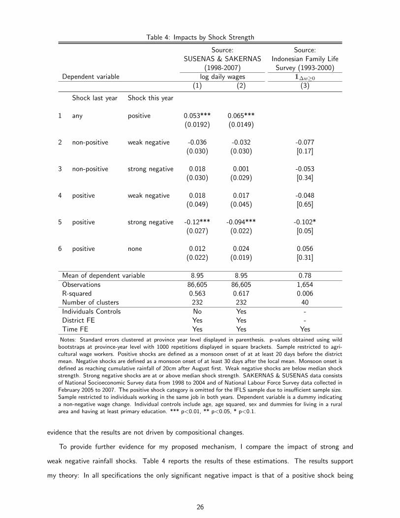
Table 4: Impacts by Shock Strength

Source: Source:SUSENAS & SAKERNAS Indonesian Family Life

(1998-2007) Survey (1993-2000)Dependent variable log daily wages 1∆w≥0

(1) (2) (3)

Shock last year Shock this year

1 any positive 0.053*** 0.065***(0.0192) (0.0149)

2 non-positive weak negative -0.036 -0.032 -0.077(0.030) (0.030) [0.17]

3 non-positive strong negative 0.018 0.001 -0.053(0.030) (0.029) [0.34]

4 positive weak negative 0.018 0.017 -0.048(0.049) (0.045) [0.65]

5 positive strong negative -0.12*** -0.094*** -0.102*(0.027) (0.022) [0.05]

6 positive none 0.012 0.024 0.056(0.022) (0.019) [0.31]

Mean of dependent variable 8.95 8.95 0.78

Observations 86,605 86,605 1,654R-squared 0.563 0.617 0.006Number of clusters 232 232 40

Individuals Controls No Yes -District FE Yes Yes -Time FE Yes Yes Yes

Notes: Standard errors clustered at province year level displayed in parenthesis. p-values obtained using wildbootstraps at province-year level with 1000 repetitions displayed in square brackets. Sample restricted to agri-cultural wage workers. Positive shocks are defined as a monsoon onset of at at least 20 days before the districtmean. Negative shocks are defined as a monsoon onset of at least 30 days after the local mean. Monsoon onset isdefined as reaching cumulative rainfall of 20cm after August first. Weak negative shocks are below median shockstrength. Strong negative shocks are at or above median shock strength. SAKERNAS & SUSENAS data consistsof National Socioeconomic Survey data from 1998 to 2004 and of National Labour Force Survey data collected inFebruary 2005 to 2007. The positive shock category is omitted for the IFLS sample due to insufficient sample size.Sample restricted to individuals working in the same job in both years. Dependent variable is a dummy indicatinga non-negative wage change. Individual controls include age, age squared, sex and dummies for living in a ruralarea and having at least primary education. *** p<0.01, ** p<0.05, * p<0.1.

evidence that the results are not driven by compositional changes.

To provide further evidence for my proposed mechanism, I compare the impact of strong and

weak negative rainfall shocks. Table 4 reports the results of these estimations. The results support

my theory: In all specifications the only significant negative impact is that of a positive shock being

26

followed by a strong negative shock. This is in line with Proposition 3, because this shock combination

has unambiguously the largest productivity gap.

Overall, my empirical findings suggest that the existence of downward nominal wage rigidity depends

on observable factors: the evidence supports the idea that wages are more likely to adjust downwards

when the cost of maintaining the wage at last period’s nominal wage is high. My results contradict full

nominal wage rigidity in agricultural labour markets as found by Kaur (2015), but at the same time my

findings support the existence of downward nominal wage rigidity when these costs are sufficiently low.

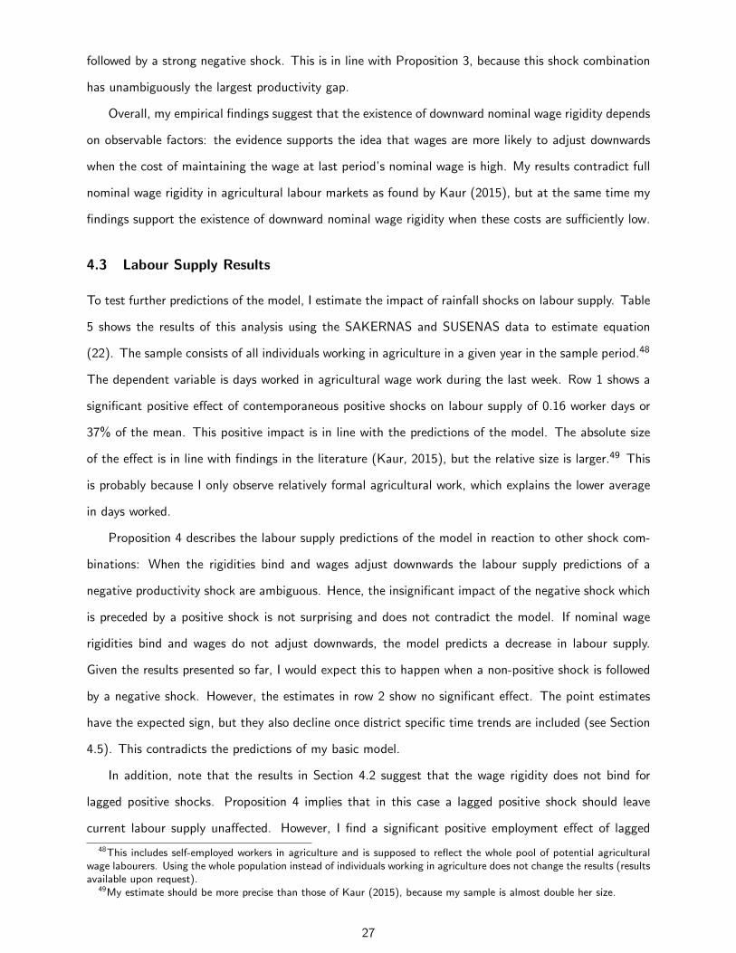
4.3 Labour Supply Results

To test further predictions of the model, I estimate the impact of rainfall shocks on labour supply. Table

5 shows the results of this analysis using the SAKERNAS and SUSENAS data to estimate equation

(22). The sample consists of all individuals working in agriculture in a given year in the sample period.48

The dependent variable is days worked in agricultural wage work during the last week. Row 1 shows a

significant positive effect of contemporaneous positive shocks on labour supply of 0.16 worker days or

37% of the mean. This positive impact is in line with the predictions of the model. The absolute size

of the effect is in line with findings in the literature (Kaur, 2015), but the relative size is larger.49 This

is probably because I only observe relatively formal agricultural work, which explains the lower average

in days worked.

Proposition 4 describes the labour supply predictions of the model in reaction to other shock com-

binations: When the rigidities bind and wages adjust downwards the labour supply predictions of a

negative productivity shock are ambiguous. Hence, the insignificant impact of the negative shock which

is preceded by a positive shock is not surprising and does not contradict the model. If nominal wage

rigidities bind and wages do not adjust downwards, the model predicts a decrease in labour supply.

Given the results presented so far, I would expect this to happen when a non-positive shock is followed

by a negative shock. However, the estimates in row 2 show no significant effect. The point estimates

have the expected sign, but they also decline once district specific time trends are included (see Section

4.5). This contradicts the predictions of my basic model.

In addition, note that the results in Section 4.2 suggest that the wage rigidity does not bind for

lagged positive shocks. Proposition 4 implies that in this case a lagged positive shock should leave

current labour supply unaffected. However, I find a significant positive employment effect of lagged

48This includes self-employed workers in agriculture and is supposed to reflect the whole pool of potential agriculturalwage labourers. Using the whole population instead of individuals working in agriculture does not change the results (resultsavailable upon request).

49My estimate should be more precise than those of Kaur (2015), because my sample is almost double her size.

27

Table 5: Labour Supply Results

Impact on worker-days in agriculture(1) (2)

Last year’s shock This year’s shock

1 any positive 0.164*** 0.164***(0.049) (0.049)

2 non-positive negative -0.076 -0.076(0.068) (0.068)

3 positive negative -0.006 -0.011(0.143) (0.143)

4 positive none 0.141** 0.139**(0.068) (0.068)

Mean of dependent variable 0.43 0.43

Observations 1,190,023 1,190,023R-squared 0.079 0.086Number of clusters 232 232

Individuals Controls No YesDistrict FE Yes YesTime FE Yes Yes

Notes: Data source is National Socioeconomic Survey from 1998 to 2004 and of National LabourForce Survey in February 2005 to 2007. Dependent variable is days worked as agricultural wageworkers. Sample restricted to individuals working in agricultural. Individual observations weightedusing cross-sectional sample weights. Positive shocks are defined as a monsoon onset of at at least20 days before the district mean. Negative shocks are defined as a monsoon onset of at least 30days after the local mean. Monsoon onset is defined as reaching cumulative rainfall of 20cm afterAugust first. Standard errors clustered at province year level displayed in parenthesis. Individualcontrols include age, age squared, sex and dummies for living in a rural area and having at leastprimary education. *** p<0.01, ** p<0.05, * p<0.1.

positive shocks of 0.14 worker days, or 32% of the mean without a corresponding increase in wages (row

4). This again contradicts the predictions of my model.

My labour supply results suggest that there are factors preventing firms from reducing employment

when the wage does not adjust downwards. One such factor could be firing frictions that make the

layoffs of workers expensive. The Indonesia Jobs Report of the World Bank (The World Bank, 2010)

asserts that employers are legally obliged to make costly severance payments to laid-off of workers. While

compliance with this law is relatively low, it could still be part of the explanation of why employment is

rigid, especially given that this analysis focuses on relatively formal agricultural workers.50

In Appendix Section A.5 I analyse the theoretical implications of including firing frictions in the

50I do not take a strong stance of what exactly causes these frictions. Alternative explanations include fairness normsover employment or implicit contracts between firms and workers.

28

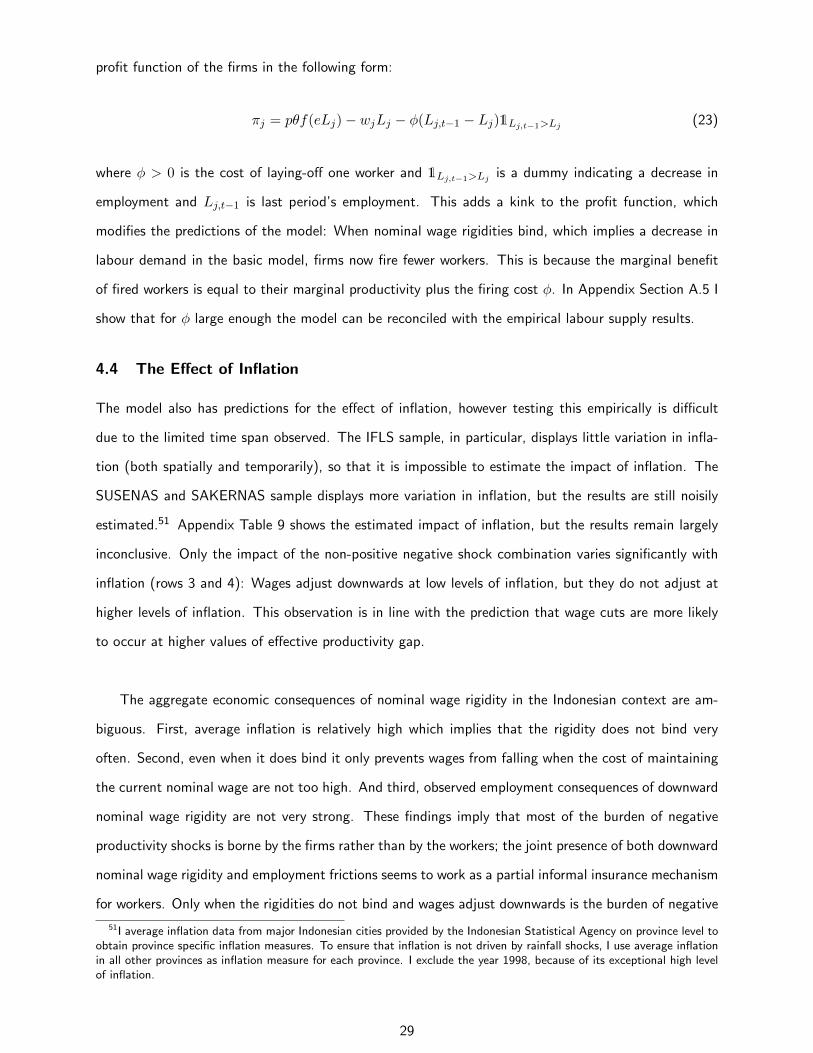
profit function of the firms in the following form:

πj = pθf(eLj)− wjLj − φ(Lj,t−1 − Lj)1Lj,t−1>Lj (23)

where φ > 0 is the cost of laying-off one worker and 1Lj,t−1>Lj is a dummy indicating a decrease in

employment and Lj,t−1 is last period’s employment. This adds a kink to the profit function, which

modifies the predictions of the model: When nominal wage rigidities bind, which implies a decrease in

labour demand in the basic model, firms now fire fewer workers. This is because the marginal benefit

of fired workers is equal to their marginal productivity plus the firing cost φ. In Appendix Section A.5 I

show that for φ large enough the model can be reconciled with the empirical labour supply results.

4.4 The Effect of Inflation

The model also has predictions for the effect of inflation, however testing this empirically is difficult

due to the limited time span observed. The IFLS sample, in particular, displays little variation in infla-

tion (both spatially and temporarily), so that it is impossible to estimate the impact of inflation. The

SUSENAS and SAKERNAS sample displays more variation in inflation, but the results are still noisily

estimated.51 Appendix Table 9 shows the estimated impact of inflation, but the results remain largely

inconclusive. Only the impact of the non-positive negative shock combination varies significantly with

inflation (rows 3 and 4): Wages adjust downwards at low levels of inflation, but they do not adjust at

higher levels of inflation. This observation is in line with the prediction that wage cuts are more likely

to occur at higher values of effective productivity gap.

The aggregate economic consequences of nominal wage rigidity in the Indonesian context are am-

biguous. First, average inflation is relatively high which implies that the rigidity does not bind very

often. Second, even when it does bind it only prevents wages from falling when the cost of maintaining

the current nominal wage are not too high. And third, observed employment consequences of downward

nominal wage rigidity are not very strong. These findings imply that most of the burden of negative

productivity shocks is borne by the firms rather than by the workers; the joint presence of both downward

nominal wage rigidity and employment frictions seems to work as a partial informal insurance mechanism

for workers. Only when the rigidities do not bind and wages adjust downwards is the burden of negative

51I average inflation data from major Indonesian cities provided by the Indonesian Statistical Agency on province level toobtain province specific inflation measures. To ensure that inflation is not driven by rainfall shocks, I use average inflationin all other provinces as inflation measure for each province. I exclude the year 1998, because of its exceptional high levelof inflation.

29

economic shocks shared between firms and workers. However, the nature of my analysis does not allow

for an explicit welfare analysis. Empirical evidence on the micro-foundations of downward nominal wage

rigidity and other labour market frictions, including experimental evidence on the presence and strength

of fairness norms in labour markets in developing countries, is needed to draw conclusions about welfare

effects.52

4.5 Ruling out Alternative Explanations

Could the observed results be caused by factors other than wage and employment rigidities? First,

in-migration following positive shocks could cause the differential impact of contemporaneous negative

shocks increasing the total labour supply.53,54 This could in theory explain the impacts of past positive

shocks on the wage reaction to contemporaneous negative shocks. However, this does not explain the

insignificant effect of negative shocks which were not preceded by a positive shock. In theory it could

be that the effects of negative productivity shocks are too weak to be detectable in the data. However,

given the strong reaction of wages to positive shocks it is implausible that negative shocks (which have a

stronger effect on productivity than positive shocks) should be too weak to influence wages. Furthermore,

when I separate negative shocks by strength the point estimates for strong negative shocks are smaller

than those for weak negative shocks (Table 4). This combined with the large sample size leave me

confident that the null effect is not caused by lack of power.55 Permanent in-migration also implies

downward pressure on wages following a lagged positive shock without a shock in the next period,

but again I do not find such an effect on wages. I cannot directly rule out that the inflow of workers

offsets positive demand spillovers caused by in-migration (Santangelo (2016) finds such spillover effects

in India). However, this is unlikely to be the case in Indonesia as Bazzi (2016) shows that wages decline

with migration inflows induced by favourable rainfall.

Second, if rainfall shocks had a permanent impact (for example by filling water depots or moisturising

52Theoretically, the ’theory of the second best’ implies that it is at least possible for firing frictions to partially offset theinefficiencies in the labour market adjustment to economic shocks caused by downward nominal wage rigidity (Lipsey, R.G. Lancaster, 1956).

53By using the IFLS data, I have already ruled out that selective migration affects the sample composition directly.54It is well-known that rainfall induces migration in Indonesia and that this migration occurs with some time lag (Bazzi,

2016). Furthermore, Rosenzweig and Udry (2014) show that the impact of rainfall shocks can be aggravated by migrationif shocks are unexpected. This in would in particular be true if rainfall shock were positively serially correlated, as workerswould expect good year to follow on another good year, which should increase the expected value of migrating to a givenlocation. However, in Appendix Table 10 I show that monsoon onset delay is negatively serially correlated in Indonesia as awhole. This means that if intertemporal optimization takes place, negative shocks should be expected to follow on positiveshocks. I workers adapted to this pattern, I would expect the serial correlation to weaken the impact of in-migration.Furthermore, I show that serial correlation disappears once time and district fixed effects are included. This means thatpast shocks in a given district have no predictive power about future shocks, once the local means and national trends areaccounted for.

55The more noisily measured result using wage change data is not surprising due to the smaller sample size and describedmeasurement issues.

30

the soil), this could explain the persistent increase of employment following a positive shock. However,

in this case wages would also remain high following a positive shock which is not the case. Similarly, if

positive shocks allowed credit-constrained farmers to invest in capital this could explain the persistent

increase in employment following a positive shock. For this to happen labour and capital would have

to be complements which implies an increase in the marginal product of labour. This would cause the

wage to increase following a lagged positive shock. However, this contradicts my empirical findings.

Permanent shocks and migration combined could explain the persistent employment effect and the

influence of past positive shocks on wage setting. However, it does, again, not explain why wages do

not fall significantly with just a negative shock.

Third, it could be that districts are on differential wage growth paths which were not accounted for

in the data. It is possible that the different shock combinations spuriously picked up these differential

trends. Appendix Table 11 shows that the cross-sectional wage rigidity results are robust to including

province and district specific linear time trends (columns 1 and 2). The positive employment effect of

lagged shocks is not fully robust to including specific time trends, but it is only marginally insignificant

when district time trends are included (column 4). Once I include district trends in the panel specification

the estimated coefficients even increase further. Clearly, the inclusion of district trends decreases power

and increases standard errors which is why these results are noisily measured.56 Thus, I can rule out

that my results are driven by differential trends.

Fourth, the definition of rainfall shocks in absolute terms causes some districts to receive either no

shocks or only one kind of shock. If for example district which only ever received a positive shock during

the period of 1979 to 2010 had systematically higher wages than districts which received a negative

shock, this could lead to spurious estimates of negative effects of negative shocks. A similar argument

can be made for district which only receive negative shocks. If districts with just negative shocks had

systematically lower wages than districts without negative shocks, this difference could be picked up by

the regression coefficient. Districts that do not receive any shock in this period are always in the control

group. For this to bias the results, wages would have to move in the opposite direction of wages districts

which experience a shock, but given the spatial correlation of monsoon onset this is relatively unlikely.

Appendix Figure C.5 shows that the spatial distribution of districts without shocks closely follows the

timing of monsoon onset. Those districts are clustered in the north west of Indonesia which means that

lack of shock coincides with different agricultural production cycle. Wages in these district are ex-ante

less likely to be affected by monsoon onset as the data collection falls into the second cropping season.

56If I cluster standard errors at the province year level, the results are significant (results available on request).

31

Hence, excluding these shocks is similar to testing for the impact by differential agricultural production

cycle. Appendix Table 12 shows that excluding districts which experienced either no shocks or only one

type of shock does not affect point estimates and results are only slightly more nosily measured.

Fifth, measurement error could contaminate the results. If measurement error was classical, my

findings would be attenuated towards zero which would strengthen the validity of my finding of partial

downward flexibility. The presence of classical measurement error would theoretically weaken the finding

of no impact of the negative shock which is not preceded by a positive shock. However, it does not

account for the differential adjustment to contemporaneous negative shocks. If wages are systematically

misreported, this could in theory bias my results in either direction. However, for this to explain the

findings, misreporting of wages would have to be correlated with intertemporal shock patterns (for

example underreporting of wages has to be more likely if a negative shock follows on a positive shock).

Furthermore, the misreporting would have to occur in both data sources in a similar fashion.

Sixth, further lags of positive shocks could potentially influence the results by defining the wage level

in the previous year. Including dummies for lagged positive shocks does not change my results for wage

level (columns 1 and 3 of Appendix Table 13). The IFLS results are a bit more noisily measured, and

the coefficient on the negative shock which is preceded by positive shock turns marginally insignificant

(column 5 of Appendix Table 13), but the general interpretation of the results is still similar. The results

are also robust to defining shocks by using a symmetric cutoff of twenty days for positive and negative

shocks (even columns of Appendix Table 13). The cross-sectional results do not change at all, while

the point estimates of both contemporaneous negative shocks increase further.

Appendix Table 14 provides further evidence that my results are not driven by selecting a specific

sample or time period. Column 1 shows that the results are robust to including wages of casual workers

for the years 2000 and 2005 to 2007 when they are reported. Column 2 shows the results excluding

observations in February 1998 when the consequences of the Asian Financial Crisis coincided with a

major drought which caused a spike in inflation and had severe economic consequences in Indonesia

(Frankenberg and Smith, 2003; Smith et al., 2002). The results confirm that my findings are not driven

by one-off effects of the crisis. The results also hold when I restrict the cross-sectional sample to districts

found in the IFLS data (column 3). Column 4 shows the results excluding the island of Sumatra from

the regression. The idea behind this is that monsoon onset is relatively early for most of the island

which could influence the results. The estimated impact of the positive negative shock combination

declines, but it still remains significant. Column 5 shows the results of the main estimation only using

32

years in which the SUSENAS are the data source.57 The positive-negative coefficient decreases slightly

and becomes marginally insignificant (with a p-value of 0.12) and the effect of the lagged positive

shock turns marginally significant. Using hourly instead of daily wages show similar results (column

6). The coefficient on the negative shock following a positive shock this time has a p-value of 0.11,

and the lagged positive coefficient becomes significant. The fact that the coefficient on lagged positive

shocks is significant in some specifications can be interpreted as further evidence supporting the idea of

downwardly rigid nominal wages.

5 Conclusion

This paper contributes to the understanding of downward nominal wage rigidity: I provide evidence that

the existence of downward nominal wage rigidity depends on observable factors which can be predicted

using economic theory. Furthermore, I propose a theoretical mechanism which is a potential explanation

for the contradictory findings of the existing casual literature on the existence of downward nominal

wage rigidity.

In particular, this paper tested for the presence of downward nominal wage rigidity in Indonesian

agricultural labour markets. I provided evidence from two separate data sources that nominal wages

exhibit differential adjustment patterns to negative labour demand shocks: when negative shocks are

not preceded by a positive shock they do not adjust downwards. However, when negative shocks follow

on a positive labour demand shock, nominal wages adjust downwards to the reduction in productivity.

Additionally, I showed that this effect is driven by differences in the cost of maintaining last period’s

nominal wage. Splitting negative productivity shocks by their severity, this paper provided further

evidence for this mechanism: wages only adjust downwards when strong negative shocks are preceded

by positive shocks, but not when weak negative shocks follow positive shocks. Furthermore, I validated

the results of a wage level analysis with an equivalent analysis using wage change data. This enabled

me to credibly deal with potential threats to identification such as selective migration or aggregation

bias.

Presenting a model of agricultural labour markets, I formalized the idea that the cost of downward

adjustment of wages determines whether nominal wages adjust to negative productivity shocks. I showed

that the cost of violating workers’ fairness norms by decreasing the nominal wage can be outweighed by

the cost of keeping nominal wages constant, which leads firms to adjust their nominal wages downwards

in some cases.

57Around 90% of my sample consists of SUSENAS data, because the SAKERNAS surveys were fairly small.

33

In addition to analysing wage-setting in response to productivity shocks, this paper also analysed the

labour supply response to labour productivity shocks. I found persistent employment effects following

positive productivity shocks and my results show no observable negative employment effect of downward

nominal wage rigidity. I augmented the model by including firing costs and proved that it is consistent

with the observed employment movements.

The results of my analysis suggest that the cost of not adjusting wages to negative productivity

shocks can explain the existence of downward nominal wage rigidity. However, to fully understand the

determinants of downward nominal wage rigidity, other potential explanations have to be considered.

In particular, analysing the impacts of duration of employment contracts and the nature of economic

shocks on downward nominal wage rigidity is a promising avenue for future research.

References

Akerlof, G. A., W. T. Dickens, G. L. Perry, R. J. Gordon, and N. G. Mankiw (1996). The Macroeconomics

of low inflation. Brookings Papers on Economic Activity 1996(1), 1–76.

Akerlof, G. A. and J. L. Yellen (1990). The Fair Wage-Effort Hypothesis and Unemployment. The

Quarterly Journal of Economics 105(2), 255–283.

Altonji, J. G. and P. J. Devereux (2000). The extent and consequences of downward nominal wage

rigidity. In Research in Labor Economics, Volume 19, pp. 383–431. Emerald Group Publishing Limited.

Barattieri, A., S. Basu, and P. Gottschalk (2014). Some Evidence on the Importance of Sticky Prices.

American Economic Journal: Macroecnomics 6(1), 70–101.

Bazzi, S. (2016). Wealth Heterogeneity and the Income Elasticity of Migration. American Economic

Journal: Applied Economics Forthcomin.

Beegle, K., C. Carletto, and K. Himelein (2012). Reliability of recall in agricultural data. Journal of

Development Economics 98(1), 34–41.

Benigno, P. and L. A. Ricci (2011). The Inflation-Output Trade-off with Downward Wage Rigidities.

American Economic Review 101(4), 1436–1466.

Bertrand, M., E. Duflo, and S. Mullainathan (2004). How Much Should We Trust Differences-in-

Differences Estimates? The Quarterly Journal of Economics 119(1), 249–275.

34

Bewley, T. F. (1995). A Depressed Labor Market as Explained by Participants. The American Economic

Review 85(2), 250–254.

Bils, M. J. (1985). Real Wages over the Business Cycle: Evidence from Panel Data. Journal of Political

Economy 93(4), 666–689.

Bound, J., C. Brown, and N. Mathiowetz (2001). Measurement error in survey data. In Handbook of

Econometrics, Volume 5, Chapter 59, pp. 3705–3843. Elsevier Masson SAS.

Bryan, G. and M. Morten (2015). Economic Development and the Spatial Allocation of Labor: Evidence

From Indonesia. Mimeo.

Cameron, a. C., J. B. Gelbach, and D. L. Miller (2008). Bootstrap-Based Improvements for Inference

with Clustered Errors. Review of Economics and Statistics 90(3), 414–427.

Card, D. (1990). Unexpected Inflation, Real Wages, and Employment Determination in Union Contracts.

The American Economic Review 80(4), 669–688.

Clarida, R. H., J. Gali, and M. Gertler (1999). The Science of Monetary Policy: A New Keynesian

Perspective. Journal of Economic Literature 37(4), 1661–1707.

Colmer, J. (2015). Weather, Labour Reallocation, and Industrial Production: Evidence from India. Job

Market Paper .

Dell, M., B. F. Jones, and B. a. Olken (2014). What Do We Learn from the Weather? The New

Climate-Economy Literature. Journal of Economic Literature 52(3), 740–798.

Dickens, W. T., L. Goette, E. L. Groshen, S. Holden, J. Messina, M. E. Schweitzer, J. Turunen, and

M. E. Ward (2007). How Wages Change: Micro Evidence from the International Wage Flexibility

Project. Journal of Economic Perspectives 21(2), 195–214.

Duncan, G. J. and D. H. Hill (1985). An Investigation of the Extent and Consequences of Measurement

Error in Labor-Economic Survey Data. Journal of Labor Economics 3(4), 508–532.

Falcon, W. P., R. L. Naylor, W. L. Smith, M. B. Burke, and E. B. McCullough (2004). Using climate

models to improve Indonesian food security. Bulletin of Indonesian Economic Studies 40(3), 355–377.

Fehr, E. and A. Falk (1999). Wage Rigidity in a Competitive Incomplete Contract Market. Journal of

Political Economy 107(1), 106–134.

35

Fehr, E., L. Goette, and C. Zehnder (2009). A Behavioral Account of the Labor Market: The Role of

Fairness Concerns. Annual Review of Economics 1(1), 355–384.

Frankenberg, E. and Karoly L (1993). The 1993 Indonesian Family Life Survey: Overview and Field

Report. Technical report, RAND, Santa Monica, CA.

Frankenberg, E. and J. P. Smith (2003). Economic Shocks , Wealth, and Welfare. The Journal of

Human Resources 38(2), 280–321.

Franklin, S. (2015). Location, search costs and youth unemployment: A randomized trial of transport

subsidies in Ethiopia. CSAE Working Paper WPS/2015-1(0).

Franklin, S. and J. Labonne (2016). Economic Shocks and Labour Market Flexibility. Mimeo.

Galı, J. (2009). Monetary Policy, Inflation, and the Business Cycle: An Introduction to the New

Keynesian Framework. Princeton University Press.

Gignoux, J. and M. Menendez (2015). Benefit in the wake of disaster: Long-run effects of earthquakes

on welfare in rural Indonesia. Journal of Development Economics 118, 26–44.

Groger, A. and Y. Zylberberg (2016). Internal Migration as a Risk-coping Strategy: Evidence from a

Typhoon. American Economic Journal: Applied Economics 8(2), 123–153.

Jayachandran, S. (2006). Selling Labor Low: Wage Responses to Productivity Shocks in Developing

Countries. Journal of Political Economy 114(3), 538–575.

Kahneman, D., J. L. Knetsch, and R. Thaler (1986). Fairness as a Constraint on Profit Seeking:

Entitlements in the Market. The American Economic Review 76(4), 728–741.

Kaur, S. (2015). Nominal Wage Rigidity in Village Labor Markets. NBER Working Paper No. 20770.

Keane, M., R. Moffitt, and D. Runkle (1988). Real Wages over the Business Cycle: Estimating the

Impact of Heterogeneity with Micro Data. Journal of Political Economy 96(6), 1232–1266.

Keane, M. P. and E. S. Prasad (1996). The Employment and Wage Effects of Oil Price Changes: A

Sectoral Analysis. Review of Economics and Statistics 78(3), 389–400.

Kirchberger, M. (2014). Natural Disasters and Labour Markets. CSAE Working Paper WPS/2014-1.

Kleemans, M. and J. Magruder (2016). Labor markets changes in response to immigration: evidence

from internal migration driven by weather shocks. Mimeo (November), 1–37.

36

LaFave, D. and D. Thomas (2014). Farms, Families, and Markets: New Evidence on Agricultural Labor

Markets. National Bureau of Economic Research No. 20699.

Levine, D. I. and D. Yang (2014). The Impact of Rainfall on Rice Output in Indonesia. NBER Working

Paper No. 20302.

Lipsey, R. G. Lancaster, K. (1956). The General Theory of Second Best. The Review of Economic

Studies 24(1), 11–32.

Maccini, S. and D. Yang (2009). Under the weather: Health, schooling, and economic consequences of

early-life rainfall. American Economic Review 99(3), 1006–1026.

Naylor, R. L., D. S. Battisti, D. J. Vimont, W. P. Falcon, and M. B. Burke (2007). Assessing risks of

climate variability and climate change for Indonesian rice agriculture. Proceedings of the National

Academy of Sciences of the United States of America 104(19), 7752–7757.

Rosenzweig, M. R. and C. Udry (2014). Rainfall forecasts, weather, and wages over the agricultural

production cycle. American Economic Review 104(5), 278–283.

Santangelo, G. (2016). Firms and Farms: The Impact of Agricultural Productivity on the Local Indian

Economy. Job Market Paper .

Smith, J. P., D. Thomas, E. Frankenberg, K. Beegle, and G. Teruel (2002). Wages, Employment and

Economic Shocks: Evidence from Indonesia. Journal of Population Economics 15(1), 161–193.

The World Bank (2010). Indonesia Jobs Report Towards Better Jobs and Security for All. Technical

report.

37