DI

SC

US

SI

ON

P

AP

ER

S

ER

IE

S

Forschungsinstitut zur Zukunft der ArbeitInstitute for the Study of Labor

The Impact of Education and Occupation onTemporary and Permanent Work Incapacity

IZA DP No. 6963

October 2012

Nabanita Datta GuptaDaniel LauDario Pozzoli

The Impact of Education and Occupation on Temporary and Permanent Work Incapacity

Nabanita Datta Gupta Aarhus University and IZA

Daniel Lau Cornell University

Dario Pozzoli

Aarhus University and IZA

Discussion Paper No. 6963 October 2012

IZA

P.O. Box 7240 53072 Bonn

Germany

Phone: +49-228-3894-0 Fax: +49-228-3894-180

E-mail: iza@iza.org

Any opinions expressed here are those of the author(s) and not those of IZA. Research published in this series may include views on policy, but the institute itself takes no institutional policy positions. The IZA research network is committed to the IZA Guiding Principles of Research Integrity. The Institute for the Study of Labor (IZA) in Bonn is a local and virtual international research center and a place of communication between science, politics and business. IZA is an independent nonprofit organization supported by Deutsche Post Foundation. The center is associated with the University of Bonn and offers a stimulating research environment through its international network, workshops and conferences, data service, project support, research visits and doctoral program. IZA engages in (i) original and internationally competitive research in all fields of labor economics, (ii) development of policy concepts, and (iii) dissemination of research results and concepts to the interested public. IZA Discussion Papers often represent preliminary work and are circulated to encourage discussion. Citation of such a paper should account for its provisional character. A revised version may be available directly from the author.

IZA Discussion Paper No. 6963 October 2012

ABSTRACT

The Impact of Education and Occupation on Temporary and Permanent Work Incapacity*

This paper investigates whether education and working in a physically demanding job causally impact temporary work incapacity, i.e. sickness absence, and permanent work incapacity, i.e. the inflow to disability via sickness absence. Our contribution is to allow endogeneity of both education and occupation by estimating a quasi-maximum-likelihood discrete factor model. Data on sickness absence and disability spells for the population of older workers come from the Danish administrative registers for 1998-2002. We generally find an independent role of both education and occupation on temporary work incapacity only. Having at least primary education reduces women’s (men’s) probability of temporary work incapacity by 16% (38%) while working in a physically demanding job increases it by 37% (26%). On the other hand, conditional on sickness absence, the effects of education and occupation on permanent work incapacity are generally insignificant. JEL Classification: I12, I20, J18, C33, C35 Keywords: work incapacity, education, occupation, factor analysis, discrete factor model Corresponding author: Dario Pozzoli Aarhus University Department of Economics and Business Fuglesangs Allé 4 8210 Aarhus Denmark E-mail: dpozzoli@asb.dk

* We would like to thank Jakob Arendt, Pilar Garcia-Gomez, Hans van Kippersluis, Petter Lundborg, Filip Pertold, David C. Ribar and Chan Shen for helpful comments and suggestions. We also appreciate comments from participants at seminars organized by Lund University, University of Maastricht, The Danish Institute of Governmental Research (AKF) and The Swedish Institute of Social Research (SOFI), and participants at the workshop on Health, Work and the Workplace, Aarhus University, May 2011, at the 32nd Nordic Health Economists Study Group Meeting, Odense, August 2011, and at the ASHE conference in Minneapolis, June 2012. Funding from the Danish Council for Independent Research-Social Sciences, Grant no.x09-064413/FSE is gratefully acknowledged. The usual disclaimer applies.

1 Introduction

Disability among working-age individuals is arguably the most important health pa-

rameter for policy purposes. Despite the impressive medical breakthroughs which have

improved aggregate health over the last decades, persistently large numbers of people

of working age leave the workforce and rely on health-related income support like sick-

ness absence and disability benefits (Autor and Duggan, 2006). This trend is witnessed

in virtually all OECD countries today, including Denmark, and the lost work effort of

these individuals represent a great cost to society.1 Health-related problems, thus, are

increasingly proving to be an obstacle to raising labor force participation rates and

keeping public expenditures under control.

Previous, mainly descriptive, research has shown a significant educational gradient

in the onset of long-term sickness absence and disability (see e.g. Fried and Guralnik,

1997, Freedman and Martin, 1999, Cutler and Lleras-Muney, 2007) and the few studies

that have estimated causal effects of education on self-reported disability status also

find significant negative effects (Kemptner et al., 2011, Oreopoulous, 2006). An occu-

pational gradient in health is also well documented (Case and Deaton, 2005; Fletcher

et al. 2009; Morefield et al. 2012; for Denmark, see Lund et al., 2004). Yet no study up

to now has tried to simultaneously uncover the relationships between these variables

and health deterioration of old workers.

1On average, expenditures on disability and sickness benefits account for about 2% of GDP inOECD countries, about 2.5 times what is spent on unemployment benefits. This ranges from 0.4%for Canada to 5% in Norway. In the US it is 1.4% of GDP, while in Denmark 3.1% of GDP is spentannually (OECD, 2005).

2

A possible theoretical basis for a socioeconomic gradient in health arising from

both education and the nature of jobs is provided in the modified version of Gross-

man’s 1972 intertemporal model of health (Muurinen, 1982; Muurinen and Le Grand,

1985; Case and Deaton, 2005). According to this theoretical setup, health deteriorates

over time but it is maintained by education through various channels. First, education

raises the efficiency of inputs needed to restore health by e.g. following directions on

medicine packages (Goldman and Lakdawalla, 2001). Second, education gives people

greater health knowledge (Kenkel, 1991). A third channel proposed by Fuchs (1982)

and Becker and Mulligan (1997) is that education can change people’s rate of time

preferences and thereby lead them to invest in better health. A final pathway between

education and health is that educated individuals can avoid physically demanding jobs

and this reduces the rate at which their health deteriorates (Muurinen, 1982, Muuri-

nen and Le Grand, 1985, Case and Deaton, 2005). That is, health is also affected

by the extent to which “health capital” is used in consumption and in work. Some

consumption activities are harder on the body than others and manual or physically

demanding work is harder on the body than non-manual work. Allowing for the health

deterioration rate to depend on physical effort provides an explanation for why health

may deteriorate faster with age among the low-educated or manual workers.

In a health care system with universal access and insurance such as the Danish one,

we would expect financial constraints to be less binding for the purpose of meeting

3

health needs. Maurer (2007) analyzes comparable cross-national data from the SHARE

on 10 European countries. Estimating health care utilization using flexible semi- and

non-parametric methods, there is no evidence of any education-related health gradient

in Denmark, and education is typically a good proxy for permanent income.2 An-

other characteristic of the Danish labor market that works against finding work-related

health-deterioration is a relatively high degree of employer accommodation paid for by

the municipalities. Danish workplaces are reportedly among the most accommodating

in Europe, especially after the twin pillars of corporate social responsibility and activa-

tion of marginalized groups were incorporated starting from the mid-1990s (Bengtsson,

2007). Larsen (2006) reports that almost half of the private and public workplaces in

Denmark with at least ten employees and with a least one employee above the age of

50 make an effort to retain older workers. These institutional features imply that any

work-related health deterioration in manual jobs found in Denmark is probably only a

lower bound of what can be found in other settings.

At the same time, prior research has convincingly shown that sickness absence and

disability are forms of moral hazard behavior in settings where agents are fully insured,

e.g. in welfare states with generous benefit provision for health-related problems (for

instance, Johansson and Palme, 2005). Compensation-seeking behavior can be of two

types: ex ante moral hazard, implying individuals do not undertake sufficient mea-

sures or investments to prevent diseases/disability or ex post moral hazard, according

2Education health gradients are found in Greece, Italy and to a certain extent in Austria andSwitzerland, but not in Spain, France, the Netherlands or Sweden. Although the results are not asclear-cut for Germany, over most of the profile the utilization appears fairly flat.

4

to which individuals claim compensation for hard to verify diseases, overplay their

symptoms or even withhold their labor supply during the awardings’ phase such as

continuing to be on sickness absence while waiting for a decision on a disability appli-

cation (Bolduc et al., 2002). In Denmark, municipalities pay for necessary workplace

adaptations, provide employers with wage subsidies and give sick-listed workers a form

of social support that facilitates continued work without risk of benefit loss. Educated

people and individuals working in non-manual jobs have lower expected payoffs from

disability insurance or sickness benefits, i.e. they would be less prone to compensation-

seeking behaviour. Although direct measures of moral hazard behavior are not present

in register data, they constitute an important source of unobserved heterogeneity that

needs to be accounted for.

The aim of this paper is to empirically model and estimate the relationships be-

tween education, working in a physically demanding job and individual health-related

exit from the labor market. More specifically, our study adds to the literature in this

field in several respects. To the best of our knowledge, this is the first attempt to

distinguish between whether lower labor market attrition among educated working-age

individuals is due to less wear-and-tear and fewer accidents on their jobs, or whether it

is due to the protective effect of education leading to greater health knowledge, more

caution and greater efficiency in health investments. Thus, our empirical analysis sin-

gles out the indirect effect of education on health working through occupational choice

from the direct effect. Second, by applying clear identification strategies based on a

5

major educational reform and on the historical characteristics of local labor supply,

we aim to uncover causal impacts of both education and working in a physically de-

manding job on sickness absence and disability. By modeling the pathway of disability

exit going through sickness absence, we also aim to explore similarities and differences

in the factors affecting behavior for these two processes. Third, to construct a highly

reliable measure of the physical demands of jobs, we use very detailed skill information

in the Dictionary of Occupational Titles (DOT) data in conjunction with the informa-

tion provided in the US census occupation codes and the Danish register’s occupation

codes.3 Furthermore, whereas much of the previous research on disability is based on

error-prone self-reported measures, we access more objective register-based indicators.

The reliability of self-reported measures has in fact been questioned because of report-

ing heterogeneity (Johns, 1994, Bago d’Uva et al., 2008, Kapetyn et al., 2007, Grøvle,

2012) as individuals may have an incentive to overplay their own health problems for

the purpose of gaining disability benefits. Finally, an important advantage of our anal-

yses is that they are carried out in a very interesting yet homogeneous setting, such

as the Danish one. Denmark has rising disability-related exit, universal health care

access and coverage and generous health benefits provision. Thus, any socioeconomic

gradient in health in Denmark cannot be due to differential access, allowing for cleaner

identification of the effects of education and occupation on health-related exit from the

labor market.

3In a sensitivity analysis, we try an alternative measure of physical demands using the DanishWork Environment Cohort Study (DWECS) data which has less detailed skill measures compared tothe DOT.

6

The comprehensiveness of the Danish register data enable us to estimate a recur-

sive model of work incapacity, education and occupation with correlated cross-equation

errors and unobserved heterogeneity. Our findings indicate that education generally

reduces sickness absence, although more strongly for men than women. At the same

time, we find an independent role for occupation, which also differs by gender. More

specifically, a stronger causal effect increasing temporary work incapacity is seen for

women than men, despite the average probability of sickness absence being fairly sim-

ilar by gender. The effects of education and occupation on permanent work incapacity

or disability, on the other hand, are generally insignificant. These results may be rele-

vant for countries with similar institutions to the Danish case, and can inform policy in

these cases of the ways in which to stem the inflow into sickness absence and disability,

respectively, temporary and permanent incapacity.

The paper is organised as follows. Section 2 introduces the data set and presents

main descriptive statistics. Section 3 provides details on the empirical strategy. Section

4 explains the results of our empirical analysis, Section 5 presents the findings from

the sensitivity analysis and Section 6 concludes.

7

2 Data

2.1 Data description

We begin with the population of individuals from 1998 to 2002. Individuals selected

for the sample are required to be employed at least in 1997 and are born in Denmark

between 1943 and 1950, which are cohorts a few years prior to and after the school

reform, that we use for our identification strategy.4 Data is taken from administrative

registers from Statistics Denmark. It is sourced from the Integrated Database for La-

bor Market Research (IDA) and includes characteristics for individuals such as highest

educational attainment, marital status, and occupation for each year. Work incapac-

ity data comes from another admistrative dataset, DREAM (Danish Register-based

Evaluation of Marginalisation), which contains information on weekly receipts of all

social transfer payments for all citizens in Denmark since 1991, and seperately records

sickness absence since 1998.

Temporary work incapacity (TWI) is defined as sickness absence for more than

eight consecutive weeks.5 This threshold is chosen as municipalities in Denmark are

4A general reform in 1958 abolished a division of schooling that occurred after the 5th grade andaffected attendance particularly beyond the 7th grade, i.e. beyond primary school. The reform alsoeliminated a distinction between rural and urban elementary schools wherein only urban schools couldoffer classes from 8th to 10th grades. The impact of the reform on individuals is based on their yearand area of birth (on the parish level). Whether the area had an urban or rural school is specifiedin the same way as in Arendt (2008). Measuring the effect on beyond primary education exploitschanges in the rural-urban difference from before to after the reform. More details about the 1958reform are reported in the next section.

5Workers can receive the benefit for up to 52 weeks, but the benefit period may be extendedunder certain circumstances, e.g. if the worker has an ongoing workers’ compensation or disabilitybenefit claim. Employers finance their workers’ sickness benefits for the first three weeks, and publicauthorities finance the remaining period.

8

obliged to follow up all cases of sickness benefit within eight weeks after the first day of

work incapacity, and aligns with other studies using Danish register data (Christensen

et al. (2008), Lund et al. (2006)) and combined survey-register data (Høgelund and

Holm (2006) and Høgelund et al. (2010)).6 If return to ordinary work is impossible

because of permanently reduced working capacity, the municipality may refer the sick-

listed worker to a wage-subsidized job, the latter being wage-subsidized jobs with tasks

accommodated to the worker’s working capacity and with reduced working hours. De-

pending on the reduction of the worker’s working capacity, the wage subsidy equals

either one half or two-thirds of the minimum wage as stipulated in the relevant collec-

tive agreement. If a person with permanently reduced working capacity is incapable of

working in a wage-subsidized job, the municipality may award a permanent disability

benefit, which is financed entirely by public authorities.

The first model, of TWI, uses the entire population of Danish workers who meet

the selection criteria stated earlier. The second model uses the full sample of indi-

viduals who experience TWI. It considers permanent work incapacity as the receipt

of disability benefit or the transit to wage-subsidized jobs, and uses data for welfare

and employment status following TWI, which is also taken from the DREAM register.

We consider the longest spell in the 24 weeks following TWI as the destination status.

The latter is grouped into four categories: permanent work incapacity, self-sufficiency,

6After the first eight weeks of sickness, the municipality must perform a follow-up assessment everyfourth week in complicated cases and every eighth week in uncomplicated cases. The primary goal ofthe assessments is to restore the sick-listed worker’s labor market attachment. The assessments musttake place in cooperation with the sick-listed worker and other relevant agents, such as the employerand medical experts.

9

early retirement and other welfare receipts (see Table 1). Permanent work incapac-

ity (PWI) includes disability benefits and wage-subsidized jobs while self-sufficiency

is largely full-time employment. 68% of the sample goes back to ordinary work after

experiencing temporary work incapacity and a considerable share (22%) transit to a

status of permanent work incapacity.

As a measure of education, we use a binary variable denoting education beyond

primary schooling (greater than 8 registered years of education). Whether or not an

individual has a physically demanding job is proxied by an occupational brawn score,

which we construct from the individual’s contemporaneous occupation codes linked to

detailed job characteristics from the U.S. Dictionary of Occupational Titles (DOT).

The fourth edition (1977) of the DOT provides measures of job content, reporting 38

job characteristics for over 12,000 occupations. Rendall (2010) performs factor analysis

on the 38 job characteristics in DOT, taken across occupations and employment from

the US 1970 census. Following Ingram (2006), Rendall arrives at 3 factors, which are

labelled brain, brawn, and motor coordination.7 We use the results of factor analysis

by Rendall (2010) on these characteristics, and obtain a single measure of brawn for

each occupational code provided in the Danish register set.

We then use crosswalks to match census occupation codes to the Danish register’s

7The orthogonal factor analysis results in three factors explaining 93 percent of the total covariance.A partition of job characteristics into the three factors is chosen, according to high coefficients from theanalysis. This partition is then used to construct a second factor analysis that allows for correlationacross factors. We sum the scores on the six variables contributing to the brawn factor, weighted bythe coefficients from factor loading, so that for each 1970 census occupation, we obtain a single valuedenoting brawn level. For more details about the factor loadings, see Table 2.

10

occupation codes, called DISCO (Danish ISCO - International Standard Classification

of Occupations). ICPSR has used the Treiman file to map from DOT to 1970 and

1980 census occupation codes. Each 1980 census occupation code in the Treiman file

carries a vector of DOT scores, which is, where applicable, an average over the 1970

codes’ scores. We use a crosswalk of 506 occupations at Ganzeboom (2003) to map

1980 census codes to ISCO-88. The 4-digit ISCO code is organised hierarchically in

four levels and is almost identical to DISCO (390 vs. 372 codes).8 The first digit aligns

broadly with the education level required for the job, and the job classification becomes

more detailed with the second and third digits. If a direct match from a DISCO code

to 1980 census code is not found, we use the nearest category, above or immediately

adjacent (based on preceding digits). One-to-many matches receive an average of the

brawn score. Over 92% of workers have an occupation code to which a brawn score

can be attributed.

We proceed with two alternative measures of physical demands of the job. One is

related only to the brawn level of the current job being above the 75th percentile of

the gender specific brawn distribution while the other is based on having a history of

brawny work in the last three years.

8http://www.dst.dk/Vejviser/Portal/loen/DISCO/DISCO-88/Introduktion.aspx

11

2.2 Variables and Descriptive Statistics

The full sample consists of 2.3 million individuals born between 1943 and 1950, em-

ployed in 1997, and subsequently observed in 1998-2002. Table 3 presents descriptive

statistics for the full sample split by gender, and within gender group, separately for

all and for the higher of the two educational groups (above primary level). Means are

taken over all person years 1998-2002 when workers are between 48 and 59 years of age.

1998 is selected as the first year because reliable information on sickness spells is only

available starting from that point on. Prior to this, sickness spells are indistinguishable

from maternity leave spells for women. Furthermore, because we are concerned about

encountering major changes in the disability policy scheme in 2003, 2002 is the last

allowable year in the sample period.

Around 3% of women and men aged 48-59 experience TWI. For those with edu-

cation beyond primary level, the corresponding shares are on average slightly lower.

Years of education are, by definition, lower for all workers compared to educated work-

ers, almost 10 years vs. 12 years. Women and men in the full sample are similar in

terms of age, the average being 53 years. Looking at the shares of workers employed

in physically demanding occupations, a striking gender difference is seen, no matter

their age (see also Figure 2). While 12% of women work in such occupations, 25% per-

cent of all men (even 13% of men with more than primary education) work in brawny

jobs, reflecting the high degree of occupational segregation by gender into, respectively,

blue-collar (male) and white-collar (female) occupations in the Danish labor market.

12

Moreover, the average brawn level in women’s commuting areas (see footnote 5) is also

considerably lower, 67, compared to 98 for men. Marriage rates among older working

women are about 2 percentage points lower than among their male counterparts. Ed-

ucated workers -both women and men-are more likely to be born in a city. The next

row in the table indirectly provides the proportion affected by the education reform

instrument, by gender and education. As approximately 26% of individuals are born

in a city after the reform year, 74% of our sample is affected by the reform. Due to

mortality risk increasing with age, there is slightly more representation of the younger

cohorts in the sample, however, differences in cohort sizes are not large.

When conditioning on TWI in Table 4, 21-23% of women and 19-21% of men are

on PWI, so the differences are not large. The TWI sample is also less educated than

the full sample but is about the same age. Those on TWI are more likely to work

in brawny jobs than those in the full sample. The brawniness of their (the TWI)

commuting area is, however, similar to that of all workers. They are also less likely

to be married compared to the full worker sample, perhaps indicative of the health

benefits that can be obtained from marriage (Wilson and Owsald, 2005). Means of

the remaining factors in this table (born in city, reform*born in city, cohort dummies)

appear to be largely the same for the TWI sub-sample as for the full sample.

13

3 Empirical strategy

Our point of departure for describing the determinants of either TWI or PWI is a set

of modified versions of Grossman’s intertemporal model of health (Muurinen, 1982;

Muurinen and Le Grand, 1985; Case and Deaton, 2005). According to this theoretical

setup, utility maximization determines the optimal level of health inputs and yields a

reduced form model of the demand of health, such as:

Hit = Xitβ + γ1Ei + γ2PJit + ξit (1)

where Hit is the health stock of individual i at time t, Xit include a number of ex-

ogenous regressors in the health equation, Ei is education, PJit is having a physically

demanding job and ξit is an error term, consisting of a time invariant vi and an idiosyn-

cratic component uit. Education may be correlated with the unobserved component

as those with better “endowment” obtain more education and are at the same time

more healthy as adults (Card, 1999; Rosenzweig and Schultz, 1983). Alternatively a

correlation between education and ξit may stem from the assumption that individu-

als with higher preferences for the future are more likely to engage in activities with

current costs and future benefits such as education and health investments (Fuchs,

1982; Grossman and Kæstner, 1997). To take account of this endogeneity issue, we

assume that education9 and the health outcome, WIit (work incapacity), in our case

9Education is measured by a dummy variable taking value of one for those having any educationbeyond primary schooling, as explained in the previous section.

14

the probability of either TWI or PWI, are related through the following equations:

WIit = X1itβ1 + γ1Ei + γ2PJit + v1i + uit

Ei = X2iβ2 + φ1URBi + φ2(URBi ∗REFi) + v2i + ηi (2)

where v1i is the time invariant unobserved component correlated with v2i but un-

correlated with X1it, which include age, age squared, gender10, whether married and

born in a urban area, the average work incapacity (TWI or PWI) annual growth rate

for each level of brawn, cohort and region of living dummies. Education is instead a

function of cohort dummies and whether born in a urban area (URBi) and whether

affected by the 1958 school reform (REFi). As in Arendt (2005, 2008), the interaction

of the urban and reform dummies constitute our exclusion restrictions. That is, the

change in urban-rural differences in education due to the 1958 reform is exploited to

identify the education effect on work incapacity. We contend that the exogenous vari-

ation in education is stronger than what is visible in the population from the number

of years of education registered (see Figure 1), for two reasons. Prior to the reform,

schooling in the 6th and 7th grades was determined on the basis of a test conducted at

the end of 5th grade. This would have led to a different schooling experience between

two sets of students in the same cohort, even when both are registered with 7 years

of education. Plus in rural schools before the reform, the curriculum level and the

number of lessons were lower. These differences were abolished in 1958, which we use

10To allow the effects of education and occupation to be gender specific, we will provide estimationresults separately for women and men.

15

to identify causal effects of increasing years of education, as well as of potentially in-

creasing quality of education, for individuals born in rural areas and from 1946 onwards.

We apply a quasi-maximum-likelihood estimator with discrete factor approxima-

tions (Mroz, 1999; Picone et al., 2003; Arendt, 2008) to estimate equation (2). The

advantages of this approach are twofold. On one hand, it is particularly suited to cor-

rect for endogeneity and selection bias caused by unmeasured explanatory variables in

dichotomous dependent-variable models (Cameron and Taber, 1998). On the other, it

avoids the need to evaluate multivariate normal integrals and it is less expensive com-

putationally. Moreover many economists have criticized IV two-stage methods (Vuong,

1984) arguing that they may deliver consistent parameter estimates with high standard

errors, making the estimates very unreliable. According to Mroz, the discrete factor

method compares favourably with efficient estimators in terms of precision and bias.

He demonstrates that the discrete factor method outperforms 2SLS in the presence of

weak instruments. Also, Staiger and Stock (1997) showed that two step approaches

are highly dependent on the quality of instruments.

To implement this estimation method, the following recursive model of work inca-

pacity (WI) and education (E) with correlated errors is considered:

WIit = f(X1itβ1 + γ1Ei + γ2PJit + v1k + uit)

Ei = g(X2iβ2 + φ1URBi + φ2(URBi ∗REFi) + v2k + ηi)

16

where uit, ηi are independently distributed and v1k and v2k represent the random

components. The latter are assumed to follow a discrete distribution pk, where pk ≥ 0

for k = 1, ...., K and∑K

k=1 pk = 1. The identification of the education effect is obtained

by the non linearity of the f(.) and g(.) functions, but it is strengthened using an

exclusion restriction. With education being binomial, the contribution to the likelihood

of a given individual is given by:

P (WIit = wiit, Ei = ei) =K∑k=1

pkP (WIit = wiit|v1k)P (Ei = ei|v2k)

Because the number of points K are unknown and there can be many local max-

ima, it is important to look for good starting values. We use single equation Probit

estimates and add one point of support for the mixing distribution at a time, doing a

grid search for the new point. We added up to three points of support. Unfortunately,

there is no standard theory indicating how to select K in a finite sample. Following

Cameron and Taber (1998) and Heckman and Singer (1984), we add additional points

of support until the likelihood fails to improve.

The previous recursive model is then extended to also tease out the causal impact

of a physically demanding job (PJ):

17

WIit = f(X1itβ1 + γ1Ei + γ2PJit + v1k + uit)

Ei = g(X2iβ2 + φ1URBi + φ2(URBi ∗REFi) + v2k + ηi)

PJit = h(X3itβ3 + δ1Ei + δ2BRAWN AV Ei + v3k + µit)

where X3it includes age, age squared and marital status. As before, the identifica-

tion of the occupation effect is obtained by the non linearity of the functions, but it is

strengthened using an exclusion restriction. As an instrument for having a physically

demanding job, we use the 1994 average brawn (separately for male and female) of

all employed individuals in the current “commuting area”.11 The average brawn at

the commuting area level presents a suitable supply driven instrument for the indi-

vidual decision to select a brawny job herself which is not correlated with the risk of

work incapacity. This argument is further reinforced by the role of networks in the

employment process (Montgomery, 1991, Munshi, 2003). Thus individuals placed in

areas with high average brawn are also more likely to have a physically demanding job.

Furthermore, it is important to emphasize that although the commuting areas are not

closed economies in the sense that workers are free to move out, there is a clear evidence

of low residential mobility for Denmark (Deding et al. 2009), which seems to support

the appropriaterness of our IV strategy. In theory, it may be preferable to use as in-

strument the brawn level of the commuting area when the individuals made their first

11The so-called functional economic regions or commuting areas are identified by using a specificalgorithm based on the following two criteria. Firstly, a group of municipalities constitute a commutingarea if the commuting within the group of municipalities is high compared to the interaction withother areas. Secondly, at least one municipality in the area must be a center, i.e. a certain share ofthe employees living in the municipality must work in the municipality, too (Andersen A. K., 2000).In total 51 commuting areas are identified.

18

job decisions, say at ages 20-25. Unfortunately, the DISCO occupational code used

to identify the commuting area average brawn is only available from 1994 onwards,

meaning that we cannot go back earlier than that for the purpose of constructing the

instrument. Furthermore, the Danish Economic Council (2002) reports that despite

low geographic mobility, the job turnover rate is quite high in Demark which means

that a significant share of individuals would have changed their jobs. Table 2 shows

the distribution of average brawn across commuting areas by gender. At the median,

the average brawn of males’ commuting areas is 45% greater than the average brawn

of females’ commuting areas.12

4 Results

4.1 Results for temporary work incapacity

We begin by exploring the effects of education and working in a physically demanding

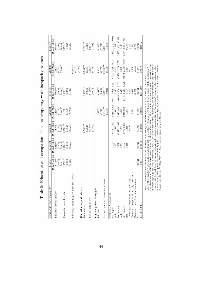
job on temporary work incapacity. In Tables 5-6, the dependent variable is tempo-

rary work incapacity (TWI), i.e., the probability of having a sickness spell of at least

8 weeks, for, respectively, women and men. Coefficient estimates from the quasi-ML

model with discrete factor approximation are shown together with standard errors.

For education and physically demanding job, we also report the calculated marginal

effects, in parentheses below. Six models (columns) are discussed in this section, while

12The correlation between having had a brawny job in the past three years and the average brawnin the commuting area is 14% for males and 9.5% for females. The correlation between the currentbrawn of individual occupation and the average brawn in the commuting area is 15% for males and13% for females.

19

the seventh is taken up in Section 5: Model 1 where both education and occupation

are treated as exogenous and time-invariant unobserved heterogeneity is not accounted

for, Model 2 the same as Model 1 but accounting for unobserved heterogeneity, Model

3 which is the same as Model 2 except that the endogeneity of education is modeled,

Model 4 the same as Model 2 but where working in a physically demanding occupation

is treated as endogenous, Model 5 in which both education and occupation are endoge-

nously determined, and finally, Model 6 which is the same as Model 5 but where an

alternate definition of occupation reflecting a past history of working in a physically

demanding job is applied in place of a current brawny occupation i.e., observed working

in a physically demanding job in the last 3 years. As clarified in the previous section,

to minimize other sources of potential endogeneity, we include only few covariates in

the specification of the main equation: age, marital status, born in a city, the average

work incapacity annual growth rate for each level of brawn, 7 cohort dummies and 14

regional dummies.

The results for women, in Table 5, are discussed first. Model 1 shows that education

exceeding primary school level reduces their likelihood of TWI significantly by 1.4pp.

Working in a physically demanding job, as expected, increases the likelihood of females

going on TWI by 1.8pp, and this effect is also statistically significant. Accounting for

time-invariant unobserved heterogeneity in Model 2 hardly changes the results and

produces, if anything, even larger effects of education and occupation on TWI.

20

In Model 3, when instrumenting education by the urban-rural difference in educa-

tion following the 1958 school reform, we see that the instrument is significantly related

to the education measure at the 5% level and shows, as expected, that the urban-rural

difference in the share attaining education beyond primary level decreased after the

reform. However, the effect of education on reducing TWI likelihood now becomes

statistically insignificant. The effect of a physically demanding job remains significant

with the same marginal effect. In Model 4, current occupation is instrumented by the

(lagged) average brawn in a worker’s commuting area while education is treated as ex-

ogenous to TWI. The average brawn is positively related to the brawniness of a female

worker’s job and is highly significant, i.e. at the 1% level. Instrumenting occupation,

as can be expected, reduces its effect on TWI and in fact, it is no longer statistically

significant.

In Model 5, both education and occupation are simultaneously instrumented for

and the results show that education (occupation) reduces (increases) the probability of

experiencing TWI and the impacts remain statistically significant. More specifically,

education exceeding primary school level reduces the likelihood of TWI by 0.5pp while

working in a physically demanding job increases the same likelihood by 1.2pp. These

marginal effects are equivalent to a decrease and a rise in the probability of TWI by

16 and 38 per cent, respectively.13 Interestingly, when computed separately by age, we

also find that the marginal effect of having a physically demanding job monotonically

13The figures are obtained using the average probability of TWI. From the estimates in Table 5, theaverage probability of TWI is approximately 3 per cent. Therefore, the changes in the probability ofTWI, in percentage terms, are (-0.005/0.032)*100=-15.625 and (0.012/0.032)*100=37.5, respectively.

21

increases with age (except for a flattening off between ages 52 and 55), as shown in

Figure 4, confirming the “broken down by work” hypothesis formulated in Case and

Deaton (2005).

What if it is not the brawniness of the current occupation but rather having a history

of brawny jobs that matters for TWI? Workers approaching the end of their careers,

particularly those experiencing health deterioration, may switch to softer “bridge” jobs

or partial retirement before retiring that may even be outside the occupation of the

career job (Ruhm, 1990). This would imply that the physical demands of the job

are erroneously proxied by current occupation brawn. However, when applying the

history-based measure of the physical demands of the job (having a brawny job in the

last three years) in Model 6, it can be seen that occupation still has a causal effect on

females’ probability of TWI, and that the marginal effect decreases slightly to 0.8pp.

Thus for women, the attributes of the current job matter more for sickness absence

than a history of physically demanding work. Presumably, this result shows that bridge

jobs are not as important a mechanism in high-wage, high labor-cost regimes where

it may be more difficult for older workers to switch jobs at the end of their careers

and/or the incentives to do so may be lower. Furthermore, Danish workplaces are said

to be among the most accommodating in the world, and the possibility to decrease

work hours or negotiate more flexible conditions would be tried before switching em-

ployment. Education remains significant in this specification.

22

Moving to the results of the effect of education and occupation on TWI for men,

in Table 6 we see in Model 1 that the effect of working in a physically demanding

occupation is slightly smaller than it is for women, increasing the chances of TWI by

0.9pp. Similar to women, education beyond primary decreases men’s likelihood of TWI

by 1.4pp. As in the case for women, accounting for time-invariant unobserved hetero-

geneity does not change the results substantially. When instrumenting education in

Model 3, the effect of education on TWI is reduced in size and the exclusion restriction

is significant and negative as we would expect. In Model 4, where occupation is endog-

enized and instrumented by the (lagged) average brawn in a worker’s commuting area,

the instrument is significant at the 1% level. Interestingly, the effect of occupation

remains significant once it is modeled as endogenous.

Proceeding to the most general specification in which both education and occupa-

tion are modeled as endogenous in Model 5, we find that both education and occupation

are statistically significant. Education exceeding primary school level reduces the like-

lihood of TWI by 1pp, while working in a physically demanding occupation has a

marginal effect, which is a little more than half as large as the effect for women, 0.7pp

compared to 1pp. However, relative to the mean, these figures are equivalent to a de-

crease and a rise in the probability of TWI by 37 and 26 per cent, respectively.14 As in

the case for women, the impact of occupation magnifies with age, as clearly indicated

in Figure 8, however, the incline is not as steep. Trying out the alternative definition of

14From the estimates in Table 7, the average probability of TWI is 2.7 per cent. There-fore, the changes in the probability of TWI, in percentage terms, are (-0.010/0.027)*100=-37 and(0.007/0.027)*100=25.9, respectively.

23

occupation based on history of physically demanding work does not change the results

for men: education remains negative and significant and occupation exerts a statisti-

cally significant effect on increasing TWI with a marginal effect of 0.5 pp.

Finally, for both men and women, in Model 6, the covariances between education

and TWI is estimated to be negative (i.e. the unobserved factors affecting a greater

tendency to go on TWI vary negatively with the unobserved factors affecting more

education), the covariance between working in a physically demanding job and TWI

is positive and the covariance between education and physically demanding job is neg-

ative, as may be expected. The negative (positive) correlation between TWI and

education (physically demanding job) could reflect the impact of unobservables such

as moral hazard behavior that was mentioned earlier.

4.2 Results for permanent work incapacity

To probe further the effects of occupation and education on work incapacity, in Ta-

bles 7 and 8 we estimate their impact on the probability of PWI (either the receipt of

disability benefits or the transit to non-regular subsidized jobs) conditional on TWI,

hence the lower sample sizes. Here too, the same six models are estimated for, respec-

tively, women and men. As was the case for TWI, the same parsimonius specification

is chosen for the equation for PWI. Besides education and occupation (and their in-

struments), only age and its square, marital status and residence in an urban area

are included as determinants. Although in principle PWI and TWI could be separate

24

processes with each their own determinants, we retain a sparse set of common deter-

minants for both mainly because our focus is on uncovering the relationships between

education, occupation and the relevant measure of work incapacity controlling for the

most obvious sources of heterogeneity and not on accounting for all the variation in

the measure of work incapacity. While the latter is certainly a worthwhile approach, it

would introduce many potentially endogenous determinants which further complicates

the analysis, given that we already are handling two sources of endogeneity simultane-

ously.

Comparing the results for women in Table 7 to Table 5, we see that in Model 1,

the estimated effect of education is stronger when the outcome is permanent work

incapacity, 4.4pp compared to 1.4pp. However, similarly to TWI, working in a physi-

cally demanding job increases this probability by 1pp. When endogenizing education

and occupation simultaneously, their effects lose significance, in spite of significant and

correctly signed instruments. The effect of occupation is not statistically significant

even in the specification based on the occupational history.15 As in Andren (2011), we

also estimate the most general specification by distinguishing between the probability

of “full time” work disability, i.e. the receipt of disability benefits, and the probability

of part-time “work disability”’, i.e. working as subsidized worker at reduced working

hours. The results are reported in columns 7 and 8 of Table 7 and hardly change

compared to the previous ones. Very similar results are found for men in Table 8, as

15Results not reported in this paper show that the impact of occupation does not even vary withage. These additional calculations are available on request from the authors.

25

the causal impact of both education and occupation are not precisely estimated.

For both men and women, in Tables 7 and 8, the cross-equation correlations between

education and PWI are estimated to be negative (i.e. the unobserved factors affecting

a greater tendency to go on PWI vary negatively with the unobserved factors affecting

more education) and the covariance between working in a physically demanding job

and PWI is positive. As earlier mentioned, a possible explanation for these plausible

correlations could be, controlling for other things, that educated people and individu-

als working in non-manual jobs have lower expected replacement rates from disability

insurance and, therefore, would be less prone to compensation-seeking behaviour.

5 Sensitivity

The results imply a significant role for our novel measure of a physically demanding

job, so we test the sensitivity of results to this measure. To this end, we run the model

using an alternative measure of brawny job based on responses to the Danish Work

Environment Cohort Study (DWECS). An index is constructed from principal compo-

nents analysis (PCA) on a subset of the workplace questions in the survey conducted

in 2005. 16

DWECS is a panel study to monitor the working population for the prevalence of

occupational risk factors. The study conducted phone interviews on physical, thermo-

16We use the 2005 survey as it includes two questions on physical exertion, where earlier surveysdo not.

26

chemical and psychosocial exposures, health and symptoms, including a doctor’s diag-

nosis, as well as self and peer assessment. It is a representative sample of the Danish

labor force. Details of the sampling are in (Burr et al., 2003, 2006). The purpose of the

DWECS survey is not to derive a complete description of the job or activities, so it is

not appropriate to use factor analysis on the entire questionnaire, as variation driven by

any factor accounts for too little of the total variation. Instead, we first select questions

about more intrinsic (objective) aspects of the job (rather than of the workplace, or

of the manager and colleagues), and these include all questions about physical activity

in the workplace. They also include aspects of job control and autonomy, and mental

or emotional demands. The first principal component accounts for almost 30 percent

of the variation, whose eigenvector reflects a brawn- like dimension. Although it is

driven by variation of jobs in relation to other jobs, rather than by fundamental tasks

or analysis of the composition of a job, it appears that the most objective questions

in the survey highlight variation in brawniness as the main dimension along which to

discriminate occupations.17

Results obtained using this alternative measure of brawny job are reported in the

last columns of Tables 5-8. In line with the main results, we find that women (men)

working in a physically demanding job have a 1.3 (0.7) percentage points higher likeli-

17The eigenvector corresponding to the first principal component is used to score each occupationfor brawn. The 61 elements in the eigenvector, each corresponding to a survey question, are theloadings given to each survey question. As most of the questions have ordered multiple choice (5 or 2)answers, we use the polychoricpca package in Stata (Kolenikov and Angeles, 2009) to derive principalcomponents from the 105 occupations for which there were at least 10 respondents. If a direct matchfrom an occupation to a DISCO code from the full sample is not found, we use the nearest category.For each individual in the full sample, the instrument of commuting area level brawn based on thenew index is generated in the same way as for the DOT-based index.

27

hood of TWI than otherwise comparable women (men).18 Furthermore, for both women

and men, the effects on the probability of PWI are imprecisely estimated, as we have

previously found in section 4, exploiting the DOT-based brawn index.

6 Conclusion

Large numbers of working age individuals continue to leave the labor force via disability

pension enroute sickness absence in almost all OECD countries today and the lost work

effort of these individuals constitute a great cost to these economies. The objective of

this paper is to empirically model the relationships between education, working in a

physically demanding job and health-related exit from the labor market with a view

to determining whether these factors have causal impacts on sickness absence and the

inflow to disability and their relative importance for each of these processes.

Theoretically, education can impact health and disability through various channels,

and one of these could be the nature of jobs. For this reason, we estimate a recursive

model of work incapacity and education and occupation with correlated cross-equation

errors and unobserved heterogeneity on comprehensive Danish longitudinal data. These

data contain objective register-based sickness absence and disability spells, unlike self-

reported measures used in the previous literature. The empirical model simultaneously

allows for endogenous education and occupation and identification is achieved by ap-

18From the estimates in Table 7 and 8, the average probability of PWI is approximately 22 per centfor both women and men. Therefore, the changes in the probability of TWI, in percentage terms, arerespectively (0.013/0.23)*100=5.65 and (0.007/0.23)*100=3.04, respectively.

28

plying as exclusion restrictions a carefully constructed measure of the physical demands

of the occupations at the commuting area level and the exogenous variation induced

by a major educational reform.

Our findings show that education (physically demanding occupation) generally re-

duces (increases) temporary work incapacity only, as the effects on permanent work

incapacity are not precisely estimated. For both men and women, education exceeding

primary school level decreases the probability of TWI, but more so for men than women

(37 versus 16 per cent). As this effect arises net of occupation, it suggests that the

extra education benefits men more, via more health knowledge, changed time rate of

preferences or greater efficiency in health investments. This is similar to the finding in

Kemptner et al. (2011) who also find that changes in compulsory schooling laws over

a 20-year period in West Germany mainly reduce the probability of long-term illness

for men but not for women.19

At the same time, we find an independent role for occupation, which also differs by

gender. More specifically, a stronger causal effect increasing temporary work incapacity

is seen for women than men (38 versus 26 per cent), despite the average probability of

TWI being fairly similar by gender. We also uncover evidence of workers in physically

demanding jobs, both men and women, being “broken down by work” over time, and

19In earlier work, Datta Gupta and Bengtsson (2012) find, using two-stage least square methods,that the educational reform significantly reduces both men and women’s disability exit, in a speci-fication which does not control for job characteristics. Thus, they do not model the endogeneity ofoccupation and nor do they estimate separate exits via sickness absence and disability.

29

women more so than men, even though the average brawn level of men’s jobs was

significantly higher. A number of explanations could be offered for the stronger effect

of a physically demanding occupation on women’s transit to sickness absence such as

biological differences in the perception of pain, a greater socialization of men to “tol-

erate” declining health and remain in the workforce or a higher degree of employer

accommodation in men’s jobs. Future work could look into which of these potential

explanations carry merit.

Our second major finding is that neither education nor the brawniness of the oc-

cupation has any effect on disability benefit receipt. One explanation could be that

conditional on being on sickness absence, disability decisions are based on strict health

and not social criteria in Denmark. However, the fact that in 2003 the programme was

reformed and the awards criteria made stricter testify perhaps to a certain laxity in the

awards system in the period before 2003, which we study. Another mechanism could

be the rise in the share of awards based on mental disorders over this period, going

from 32.1% of all grants in 2001 to 44.4% in 2006 and a decline in the share of grants

based on musculo-skeletal disorders implying a decreasing role for occupational brawn.

Recall that the factor analysis based on DWECS data included questions relating to

job control and autonomy, and mental or emotional demands in addition to physical

demands. However, occupations distinguished themselves most from each other in the

DWECS according to a brawn-like aspect. A remaining explanation for the lack of an

effect of brawn on permanent work incapacity could be greater workplace accommo-

30

dation and efforts to retain workers in Danish workplaces. Finally, several robustness

checks on the definition of work incapacity and physically demanding job confirmed

the results above.

31

References

[1] Andersen, Anne K., 2000. “Commuting Areas in Denmark”, Copenhagen, AKF

forlaget.

[2] Arendt, J. N., 2008. “In Sickness and in Health- Till Education do us Part: Ed-

ucation Effects on Hospitalization”, The Economics of Education Review, 27(2):

161-172.

[3] Andren, D., 2011. “Half empty of half full: The importance of the definition of

part-time sick leave when estimating its effects”, Orebro University working paper,

4/2011.

[4] Autor, D. H., and Duggan M.G., 2006. “The Growth in the Social Security Dis-

ability Rolls: A Fiscal Crisis Unfolding”, Journal of Economic Perspectives 20(3):

71-96.

[5] Bago d’Uva, T., van Doorslaer, E., Lindeboom, M. and O Donnell, O. 2007. “Does

reporting heterogeneity bias the measurement of health disparities?”, Health Eco-

nomics, 17.

[6] Becker, G. S. and C.B. Mulligan, 1997. “The Endogenous Determination of Time

Preference”, Quarterly Journal of Economics, 112: 729-758.

[7] Bengtsson, S. Report on the Employment of Disabled Persons in European Coun-

tries, Country: Denmark. The Academic Network of European Disability Experts

(ANED) 2007; VT/2007/005

32

[8] Bolduc, D., Fortin B., Labrecque F., and Lanoie P., 2002. “Workers’ Compensa-

tion, Moral Hazard and Composition of Workplace Injuries”, Journal of Human

Resources 37(3):623-652.

[9] Burr H, Bjorner JB, Kristensen TS, et al., 2003. “Trends in the Danish work

environment in 1990-2000 and their associations with labor-force changes”, Scand

J Work Environ Health 29.

[10] Burr, H., Bach, E., Gram, H. and Villadsen, E., 2006.

“Arbejdsmiljo i Danmark 2005 - et overblik fra den Na-

tionale Arbejdsmiljøkohorte”, Kobenhavn, Arbejdsmiljø instituttet

http://www.arbejdsmiljoforskning.dk/ /media/Arbejdsmiljoedata/NAK/nak2005-

arbejdsmiljoe.pdf

[11] Cameron, S. and C. Taber, 1998. “Discount Rate Bias in the Returns to School-

ing”, Nothwestern U

[12] Card, D., 1999. “Causal effects of education on earnings”. Handbook of labor

economics 3 A: 1801-1863.

[13] Case, A. and Deaton, A., 2005. “Broken Down by Work and Sex: How Our

Health Declines”, in David A. Wise, editor, “Analyses in the Economics of Aging”

University of Chicago Press.

[14] Christensen KB, Labriola M, Kivimaki M, Lund T., 2008. “Explaining the social

gradient in long-term sickness absence: a prospective study of Danish employees”,

J Epidemiol Community Health. 62.

33

[15] Cutler, D.M. and Lleras-Muney, A., 2006. “Education and Health: Evaluating

Theories and Evidence”, NBER Working Paper, no. 12352.

[16] Cutler, D.M. and Lleras-Muney, A., 2007. “The Education Gradient in Old-age

Disability”, NBER forthcoming chapter in the Research Findings in the Economics

of Aging.

[17] Datta Gupta, N. and Bengtsson, S. “The Stronger Sex? The Effect of Compulsory

Schooling Reforms on Gender Differences in Disability Exit”, mimeo, University

of Aarhus.

[18] Deding, M., Filges, T. and Jos Van Ommeren, 2009. “Spatial Mobility and Com-

muting: the Case of Two-Earner Households”, Journal of Regional Science 49:

113-47.

[19] Deding, M. and Filges, T., 2009. “Danske lønmodtagers arbejdstid - En regis-

teranalyse baseret p̊a lønstatistikken (Working hours of Danish Employees - A

Register Analysis based on the Wage Statistics)”, SFI Working Paper, 09-03.

[20] Fletcher, J. M., Sindelarn J., and Yamaguchi S., (Forthcoming). “Cumulative

effects of job characteristics on health”, Health Economics.

[21] Freedman, V.A. and Martin, L.G., 1999. “The Role of Education in Explaining

and Forecasting Trends in Functional Limitations among Older Americans”, De-

mography, 36(4):461-473.

34

[22] Fried, L.P. and Guralnik, J.M., 1997. “Disability and Older Adults: Evidence

regarding Significance, Etiology and Risk”. Journal of American Geriatric Society,

45:92-100.

[23] Fuchs, V., 1982. “Time Preference and Health: An Exploratory Study”. In Fuchs

(ed.) Economic Aspects of Health: Second NBER Conference in Standford. Uni-

versity of Chicago Press, Chicago, 93-119.

[24] Ganzeboom, Harry B.G.; Treiman, Donald J., 2003. “Inter-

national Stratification and Mobility File: Conversion Tools”,

http://home.fsw.vu.nl/hbg.ganzeboom/ismf/occisko. (26.2.03)

[25] Goldman, D.P. and Lakdawalla, D., 2001. “Understanding Health Disparities

across Education Groups”, NBER Working Paper, no. 8328.

[26] Grossman, M., 1972. “On the Concept of Health Capital and the Demand for

Health”, Journal of Political Economy 80(2): 223-255

[27] Grossman, M., and Kæstner, R., 1997. “The Effects of Education on Health”, The

Social Benefits of Education, MI: 69-123.

[28] Grøvle, L. et al., 2012. “Poor agreement found between self-report and a public

registry on duration of sickness absence”, Journal of Clinical Epidemiology, 65,

212-218.

35

[29] Heckman J. and B. Singer, 1984. “ A Method for Minimizing the Impact of Distri-

butional Assumptions in Econometric Models for Duration Data”, Econometrica,

52(2): 271-320.

[30] Høgelund, J. and Holm, A. “Case management interviews and the return to work

of disabled employees”, Journal of Health Economics. 2006;25(3):500-519

[31] Høgelund, Jan and Holm, Anders and McIntosh, James, 2010. “Does graded

return-to-work improve sick-listed workers’ chance of returning to regular working

hours?”, Journal of Health Economics, Elsevier, vol. 29(1): 158-169.

[32] Ingram, B.F. and G.R. Neumann, 2006. “The returns to Skill”, labor Economics,

13(1), 35-59.

[33] Larsen, M. 2006. “Fastholdelse og rekruttering af ældre. Arbejdspladsers indsats.

(Retaining and Recruiting the Elderly: Workplace Interventions)”, (Copenhagen:

The Danish National Centre for Social Research), WP 06: 09.

[34] Johansson, P., Palme, M. 2005. “Moral hazard and sickness insurance”, Journal

of Public Economics, 89: 1879-1890.

[35] Johns, G., 1994. “How often were you absent? A review of the use of self-reported

absence data”, Journal of Applied Psychology, 79, 574-591.

[36] Kenkel, D., 1991. “Health Behavior, Health Knowledge and Schooling”, Journal

of Political Economy 99: 287-305.

36

[37] Kemptner, D. H., Jurges, H. and Reinhold, S., 2011. “Changes in compulsory

schooling and the causal effect of education on health: Evidence from Germany”,

Journal of Health Economics, 30(2):340-354.

[38] Kolenikov, S., and G. Angeles, 2009. “Socioeconomic Status Measurement With

Discrete Proxy Variables: Is Principal Component Analysis A Reliable Answer?”,

Review of Income and Wealth, 55(1), 128-165.

[39] Lund T, Labriola M, Christensen KB, et al. 2006. “Physical work environment

risk factors for long term sickness: prospective findings among a cohort of 5357

employees in Denmark”, BMJ 332:449-52.

[40] Maurer, J., Socioeconomic and Health Determinants of Health Care Utilization

Among Elderly Europeans: A New Look at Equity, Intensity and Responsiveness

in Ten European Countries HEDG Working Paper 07/26

[41] Montgomery, James D., 1991. “Social Networks and Labor Market Outcomes:

Toward an Economic Analysis”, American Economic Review 81: 1408-18.

[42] Morefield, B., Ribar, D. and Ruhm, C., 2012 “Occupational Status and Health

Transitions”, The B.E. Journal of Economic Analysis & Policy, 11, 3.

[43] Mroz, T., 1999. “Discrete Factor Approximations in Simultaneous Equations Mod-

els: Estimating the Impact of a Dummy Endogenous Variable on a Continuous

Outcome”, Journal of Econometrics, 72(2), 233-274.

37

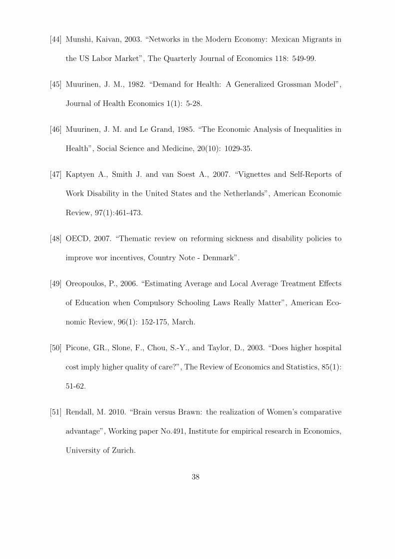
[44] Munshi, Kaivan, 2003. “Networks in the Modern Economy: Mexican Migrants in

the US Labor Market”, The Quarterly Journal of Economics 118: 549-99.

[45] Muurinen, J. M., 1982. “Demand for Health: A Generalized Grossman Model”,

Journal of Health Economics 1(1): 5-28.

[46] Muurinen, J. M. and Le Grand, 1985. “The Economic Analysis of Inequalities in

Health”, Social Science and Medicine, 20(10): 1029-35.

[47] Kaptyen A., Smith J. and van Soest A., 2007. “Vignettes and Self-Reports of

Work Disability in the United States and the Netherlands”, American Economic

Review, 97(1):461-473.

[48] OECD, 2007. “Thematic review on reforming sickness and disability policies to

improve wor incentives, Country Note - Denmark”.

[49] Oreopoulos, P., 2006. “Estimating Average and Local Average Treatment Effects

of Education when Compulsory Schooling Laws Really Matter”, American Eco-

nomic Review, 96(1): 152-175, March.

[50] Picone, GR., Slone, F., Chou, S.-Y., and Taylor, D., 2003. “Does higher hospital

cost imply higher quality of care?”, The Review of Economics and Statistics, 85(1):

51-62.

[51] Rendall, M. 2010. “Brain versus Brawn: the realization of Women’s comparative

advantage”, Working paper No.491, Institute for empirical research in Economics,

University of Zurich.

38

[52] Rosenzweig, M. R., and Schultz, T., P., 1983. “Estimating a Household Production

Function: Heterogeneity, the Demand for Health Inputs and their Effects on Birth

Weight”, The Journal of Political Economy, 91(5): 723-746.

[53] Ruhm, C. J, 1990. “Bridge Jobs and Partial Retirement”, Journal of Labor Eco-

nomics, 8(4): 482-501.

[54] Stock, J. H. and Yogo M., 2005. “Testing for weak instruments in linear IV re-

gression”, In D.W.K. Andrews and J.H. Stock (eds.), Identification and inference

for econometric models: Essays in honour of Thomas Rothenberg, Cambridge:

Cambridge University Press.

[55] The Danish Economic Council, 2002. “Den geografisk mobilitet p̊a arbejds-

markedet (Geographic mobility on the labor market)”, Fall 2002 report, Chapter

IV.

[56] Vuong, Q. H. (1984). “Two-stage Conditional Maximum Likelihood Estimation of

Econometric Models”, Social Science Working Paper 538, California Institute of

Technology.

[57] Wilson, C. M. and Oswald, A. J. (2005). “How Does Marriage Affect Physical

and Psychological Health? A Survey of the Longitudinal Evidence”, The War-

wick Economics Research Paper Series (TWERPS) 728, University of Warwick,

Department of Economics.

39

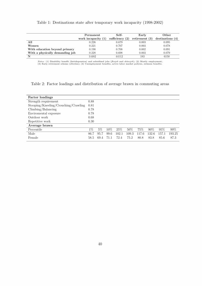
Table 1: Destinations state after temporary work incapacity (1998-2002)

Permanentwork incapacity (1)

Self-sufficiency (2)

Earlyretirement (3)

Otherdestinations (4)

All 0.226 0.679 0.003 0.095Women 0.221 0.707 0.003 0.078With education beyond primary 0.198 0.708 0.002 0.091With a physically demanding job 0.228 0.698 0.003 0.079N 14482 44112 183 6150

Notes: (1) Disability benefit (førtidspension) and subsidized jobs (flexjob and sk̊anejob); (2) Mostly employment;(3) Early retirement scheme (efterløn); (4) Unemployment benefits, active labor market policies, sickness benefits.

Table 2: Factor loadings and distribution of average brawn in commuting areas

Factor loadingsStrength requirement 0.88Stooping/Kneeling/Crouching/Crawling 0.81Climbing/Balancing 0.78Enviromental exposure 0.78Outdoor work 0.68Repetitive work 0.30Average brawnPercentile 1% 5% 10% 25% 50% 75% 90% 95% 99%Male 86.7 95.7 99.6 102.1 109.3 117.6 132.6 157.1 193.25Female 58.5 69.4 71.1 72.4 75.2 80.8 83.8 85.6 87.3

40

Table 3: Descriptive statistics of the all sample

Women MenVariables: All Education beyond primary All Education beyond primaryTemporary work incapacity 0.0340 0.0281 0.0283 0.0202Years of education 10.7272 12.0451 10.8406 12.5959Education beyond primary 0.5918 0.4855Age 53.3294 53.1016 53.4342 53.2460Physically demanding job 0.1198 0.0818 0.2477 0.1274Average brawn at the commuting area 67.4503 66.57455 97.8857 96.0558Married 0.7493 0.7402 0.7735 0.7857Born in city 0.4069 0.4681 0.4043 0.4898Reform*Born in city 0.2684 0.3180 0.2602 0.3245Cohort (1943) 0.0996 0.0851 0.1075 0.0947Cohort (1944) 0.1138 0.1002 0.1207 0.1098Cohort (1945) 0.1258 0.1152 0.1313 0.1218Cohort (1946) 0.1352 0.1308 0.1384 0.1353Cohort (1947) 0.1381 0.1362 0.1344 0.1338Cohort (1948) 0.1318 0.1372 0.1272 0.1337Cohort (1949) 0.1265 0.1410 0.1203 0.1303Cohort (1950) 0.1293 0.1542 0.1203 0.1406N 1105809 647598 1230614 597433

Table 4: Descriptive statistics of the sample of individuals with temporary work inca-pacity

Women MenVariables: All Education beyond primary All Education beyond primaryPermanent work incapacity 0.2349 0.2059 0.2219 0.1904Years of education 10.1411 11.7620 9.8879 11.7150Education beyond primary 0.2256 0.1636Age 53.7681 53.8967 53.8150 54.0297Physically demanding job 0.1711 0.1298 0.3457 0.2148Average brawn at the commuting area 67.9019 66.8856 99.1773 97.0483Married 0.7142 0.6510 0.7262 0.7442Born in city 0.3985 0.4737 0.3810 0.4672Reform*Born in city 0.2591 0.3143 0.2352 0.2918Cohort (1943) 0.1008 0.0948 0.1216 0.1161Cohort (1944) 0.1199 0.1075 0.1313 0.1249Cohort (1945) 0.1308 0.1167 0.1362 0.1326Cohort (1946) 0.1362 0.1377 0.1430 0.1458Cohort (1947) 0.1406 0.1403 0.1327 0.1499Cohort (1948) 0.1266 0.1279 0.1179 0.1157Cohort (1949) 0.1232 0.1305 0.1104 0.1149Cohort (1950) 0.1220 0.1446 0.1070 0.1001N 33297 16027 31760 10593

41

Figure 1: The school reform and the share of individuals with at least primary education

Notes: Trends before and after the school reform are calculated with a quadratic fit.

42

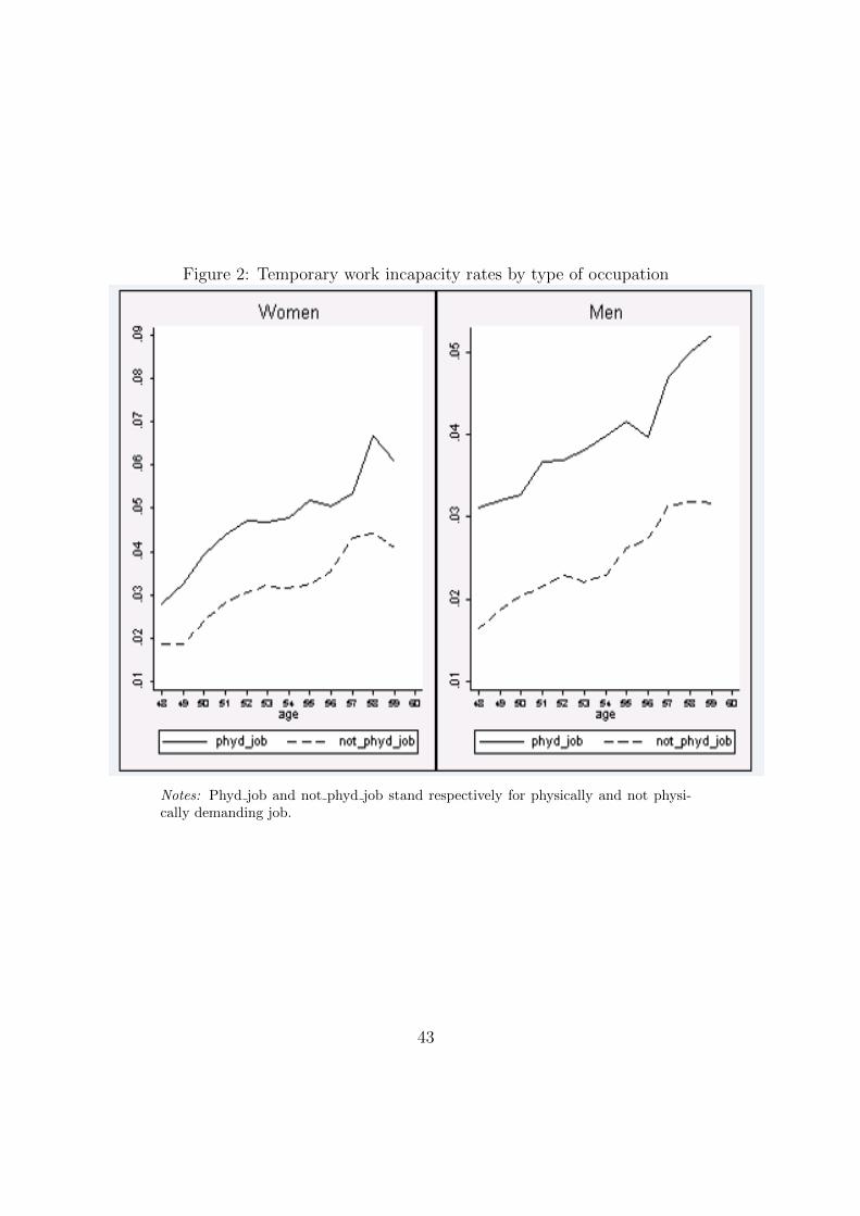
Figure 2: Temporary work incapacity rates by type of occupation

Notes: Phyd job and not phyd job stand respectively for physically and not physi-cally demanding job.

43

Tab

le5:

Educa

tion

and

occ

upat

ion

effec

tson

tem

por

ary

wor

kin

capac

ity,

wom

en

Tem

pora

ryw

ork

inca

paci

tyM

od

el1

Mod

el2

Mod

el3

Mod

el4

Mod

el5

Mod

el6

Mod

el7

(S.E

.)[M

.E.]

(S.E

.)[M

.E.]

(S.E

.)[M

.E.]

(S.E

.)[M

.E.]

(S.E

.)[M

.E.]

(S.E

.)[M

.E.]

(S.E

.)[M

.E.]

Educa

tion

bey

ond

pri

mar

y–0

.188

***

–0.2

25**

*–0

.102

–0.2

15**

*–0

.065

***

–0.0

89**

*–0

.079

***

(0.0

06)

(0.0

07)

(0.0

75)

(0.0

06)

(0.0

14)

(0.0

17)

(0.0

17)

[-0.014]

[-0.016]

[-0.007]

[-0.015]

[-0.005]

[-0.006]

[-0.006]

Physi

cally

dem

andin

gjo

b0.

151*

**0.

178*

**0.

153*

**0.

007

0.13

6***

0.15

1***

(0.0

08)

(0.0

09)

(0.0

07)

(0.0

21)

(0.0

22)

(0.0

07)

[0.013]

[0.014]

[0.013]

[0.0001]

[0.012]

[0.013]

Physi

cally

dem

andin

gjo

bin

the

last

3ye

ars

0.10

5***

(0.0

07)

[0.008]

Ed

uca

tion

beyon

dp

rim

ary

Bor

nin

city

0.54

8***

0.49

3***

0.54

3***

0.30

1***

(0.0

81)

(0.0

15)

(0.0

41)

(0.0

48)

Ref

orm

*Bor

nin

city

–0.1

40**

–0.1

40**

*–0

.149

***

–0.1

54**

(0.0

67)

(0.0

19)

(0.0

49)

(0.0

58)

Physi

call

yd

em

an

din

gjo

bE

duca

tion

–0.4

20**

*–0

.164

***

–1.9

04**

*–0

.796

***

(0.0

12)

(0.0

17)

(0.0

55)

(0.2

27)

Ave

rage

bra

wn

atth

eco

mm

uti

ng

area

0.01

4***

0.01

5***

0.01

8***

0.19

9***

(0.0

01)

(0.0

01)

(0.0

00)

(0.0

03)

Unobserved

heterogeneity

1st

supp

ort

-1.0

12-0

.513

,-4

.322

-1.2

23;

-1.1

080.

087,

-7.0

04,

-0.3

930.

416,

-3.7

16,

-0.2

27-0

.215

,-3

.242

,-0

.003

pro

b0.

295

0.41

50.

482

0.34

60.

431

0.65

12n

dsu

pp

ort

0.93

1-0

.171

,2.

948

0.94

0;3.

801

-0.0

54,

4.48

6,0.

216

-0.4

22,

2.27

0,3.

579

0.49

5,2.

691,

-0.8

61pro

b0.

273

0.25

30.

123

0.53

50.

103

0.11

03r

dsu

pp

ort

0.10

20.

775,

3.17

61.

203;

0.16

7-0

.007

,3.

537,

-0.5

20-0

.292

,2.

945,

-0.5

870.

357,

1.90

0,7.

581

pro

b0.

431

0.33

10.

394

0.11

70.

464

0.23

95C

ovar

iance

(tem

p.

wor

kin

c.,

educa

tion

)-0

.610

-0.3

44-0

.117

-0.2

48C

ovar

iance

(tem

p.

wor

kin

c.,

phy.

dem

.jo

b)

1.17

40.

022

0.76

60.

030

Cov

aria

nce

(phy.

dem

.jo

b,

educa

tion

)-0

.205

-0.4

04-0

.995

N91

0763

9107

6391

0763

9107

6391

0763

9107

6391

0763

Pse

udo

R2;

LL

0.01

9–1

2895

4.6

–283

223.

6–2

6900

6.3

-473

715.

92-6

5595

9.1

-733

491.

7

Note

s:T

he

dep

endent

vari

able

isth

epro

babilit

yof

havin

ga

sickness

spell

of

at

least

8w

eeks.

Incolu

mns

1,2

,3,4

,5and

6,

the

vari

able

”physi

cally

dem

andin

gjo

b”

isconst

ructe

don

aD

OT

-base

dbra

wn

index,

while

incolu

mn

7is

calc

ula

ted

on

aD

WE

CS-b

ase

dbra

wn

index.

Inall

specifi

cati

ons:

i)th

e”te

mp

ora

ryw

ork

incapacit

y”

equati

on

als

oin

clu

des

age,

age

square

d,

a”m

arr

ied”

and

a”b

orn

ina

urb

an

are

a”

dum

mie

s,th

eavera

ge

work

incapacit

yannual

gro

wth

rate

for

each

level

of

bra

wn,

cohort

and

regio

nal

dum

mie

s;ii

)th

e”educati

on”

equati

on

als

oin

clu

des

cohort

dum

mie

s;iii)

the

”physi

cally

dem

andin

gjo

b”

equati

on

als

oin

clu

des

age,

age

square

dand

a”m

arr

ied”

dum

my.

Sig

nifi

cance

levels

:***1%

,**5%

,*10%

,st

andard

err

ors

inpare

nth

ese

s.

44

Tab

le6:

Educa

tion

and

occ

upat

ion

effec

tson

tem

por

ary

wor

kin

capac

ity,

men

Tem

pora

ryw

ork

inca

paci

tyM

od

el1

Mod

el2

Mod

el3

Mod

el4

Mod

el5

Mod

el6

Mod

el7

(S.E

.)[M

.E.]

(S.E

.)[M

.E.]

(S.E

.)[M

.E.]

(S.E

.)[M

.E.]

(S.E

.)[M

.E.]

(S.E

.)[M

.E.]

(S.E

.)[M

.E.]

Ed

uca

tion

bey

ond

pri

mar

y–0

.224

***

–0.2

82**

*-0

.193

***

–0.2

88**

*–0

.156

***

–0.0

54**

*–0

.123

***

(0.0

06)

(0.0

08)

(0.0

07)

(0.0

07)

(0.0

07)

(0.0

11)

(0.0

14)

[-0.014]

[-0.018]

[-0.013]

[-0.018]

[-0.010]

[-0.004]

[-0.007]

Physi

call

yd

eman

din

gjo

b0.

174*

**0.

178*

**0.

171*

**0.

146*

*0.

131*

**0.

120*

**(0

.007

)(0

.008

)(0

.007

)(0

.015

)(0

.015

)(0

.015

)[0.009]

[0.011]

[0.009]

[0.007]

[0.007]

[0.007]

Physi

call

yd

eman

din

gjo

bin

the

last

3ye

ars

0.09

4***

(0.0

17)

[0.005]

Ed

uca

tion

beyon

dp

rim

ary

Bor

nin

city

0.25

1**

0.21

5***

0.47

6***

0.44

4***

(0.0

88)

(0.0

59)

(0.0

11)

(0.0

13)

Ref

orm

*Bor

nin

city

–0.2

16**

–0.2

18**

–0.0

90**

*–0

.048

**(0

.091

)(0

.072

)(0

.013

)(0

.016

)P

hysi

call

yd

em

an

din

gjo

bE

du

cati

on–0

.843

***

–1.7

57**

*–1

.223

**–1

.007

***

(0.0

11)

(0.5

26)

(0.5

26)

(0.0

14)

Ave

rage

bra

wn

atth

eco

mm

uti

ng

area

0.01

0***

0.00

9***

0.02

2***

0.02

9***

(0.0

00)

(0.0

00)

(0.0

01)

(0.0

06)

Unobserved

heterogeneity

1st

sup

por

t-0

.948

0.21

3,-3

.328

-1.0

40,

0.81

0-0

.328

,-3

.006

,-1

.891

0.09

1,-5

.757

,-0

.763

0.05

9,-5

.639

,-0

.449

pro

b0.

304

0.27

70.

475

0.32

20.

333

0.61

2nd

sup

por

t1.

122

-1.1

19,

3.88

31.

057,

-1.8

250.

398,

3.73

1,1.

605

0.08

7,-0

.541

,2.

924

0.01

5,-0

.548

,2.

843

pro

b0.

256

0.48

40.

245

0.48

50.

236

0.16

53r

dsu

pp

ort

0.0

032.

029,

-4.0

173.

310,

0.19

9-0

.456

,0.

620,

-4.3

77-0

.118

,4.

754,

-1.0

10-0

.173

,15

.735

,-0

.875

pro

b0.

439

0.23

80.

278

0.19

20.

431

0.22

4C

ovar

ian

ce(t

emp

.w

ork

inc.

,ed

uca

tion

)-0

.241

-0.4

23-0

.430

-0.8

21C

ovar

ian

ce(t

emp

.w

ork

inc.

,p

hy.

dem

.jo

b)

1.61

91.

179

0.08

80.

924

Cov

aria

nce

(phy.

dem

.jo

b,

edu

cati

on)

-0.6

06-0

.978

-1.8

02N

9598

9995

9899

9598

9995

9899

9598

9995

9899

9598

99P

seu

do

R2;

LL

0.01

7–1

1756

0.1

–288

485.

1–3

6608

3.0

–623

798.

6–6

5620

2.4

–634

045.

9

Note

s:T

he

dep

endent

vari

able

isth

epro

babilit

yof

havin

ga

sickness

spell

of

at

least

8w

eeks.

Incolu

mns

1,2

,3,4

,5and

6,

the

vari

able

”physi

cally

dem

andin

gjo

b”

isconst

ructe

don

aD

OT

-base

dbra

wn

index,

while

incolu

mn

7is

calc

ula

ted

on

aD

WE

CS-b

ase

dbra

wn

index.

Inall

specifi

cati

ons:

i)th

e”te

mp

ora

ryw

ork

incapacit

y”

equati

on

als

oin

clu

des

age,

age

square

d,

a”m

arr

ied”

and

a”b

orn

ina

urb

an

are

a”

dum

mie

s,th

eavera

ge

work

incapacit

yannual

gro

wth

rate

for

each

level

of

bra

wn,

cohort

and

regio

nal

dum

mie

s;ii

)th

e”educati

on”

equati

on

als

oin

clu

des

cohort

dum

mie

s;iii)

the

”physi

cally

dem

andin

gjo

b”

equati

on

als

oin

clu

des

age,

age

square

dand

a”m

arr

ied”

dum

my.

Sig

nifi

cance

levels

:***1%

,**5%

,*10%

,st

andard

err

ors

inpare

nth

ese

s.

45

Figure 3: Marginal effects of physically demanding job on temporary work incapacityby age, women

.01

.01

5.0

2.0

25

Ma

rgin

al effe

ct of p

hysic

ally

de

man

din

g job

48 49 50 51 52 53 54 55 56 57 58 59 60age

46

Figure 4: Marginal effects of physically demanding job on temporary work incapacityby age, men

.00

6.0

08

.01

.01

2.0

14

Ma

rgin

al effe

ct of p

hysic

ally

de

man

din

g job

48 49 50 51 52 53 54 55 56 57 58 59 60age

47

Tab

le7:

Educa

tion

and

occ

upat

ion

effec

tson

per

man

ent

wor

kin

capac

ity,

wom

en

Perm

anent

work

inca

paci

tyM

odel1

Model2

Model3

Model4

Model5

Model6

Model7

Model8

Model9

(S.E

.)[M

.E.]

(S.E

.)[M

.E.]

(S.E

.)[M

.E.]

(S.E

.)[M

.E.]

(S.E

.)[M

.E.]

(S.E

.)[M

.E.]

(S.E

.)[M

.E.]

(S.E

.)[M

.E.]

(S.E

.)[M

.E.]

Educa

tion

bey

ond

pri

mar

y–0

.146

***

–0.1

50**

*–0

.126

–0.1

28**

*–0

.056

–0.1

06–0

.062

–0.0

82–0

.051

(0.0

17)

(0.0

18)

(0.1

25)

(0.0

19)

(0.0

29)

(0.0

58)

(0.0

34)

(0.3

06)

(0.0

37)

[–0.04

4][–0.04

4][–0.03

3][–0.03

9][–0.01

6][-0.02

2][–0.01

6][-0.01

8][–0.01

6]P

hysi

cally

dem

andin

gjo

b0.

031

0.03

20.

031

0.02

60.

028

0.01

80.

010

0.03

1(0

.023

)(0

.023

)(0

.022

)(0

.029

)(0

.024

)(0

.025

)(0

.037

)(0

.077

)[0.010

][0.010

][0.010

][0.008

][0.009

][0.015

][0.004

][0.010

]P

hysi

cally

dem

andin

gjo

bin

the

last

3ye

ars

0.01

6(0

.042

)[0.004

]E

duca

tion

beyond

pri

mary

Bor

nin

city

4.57

3***

4.32

3***

3.71

8***

4.26

5***

4.40

0***

4.51

4***

(1.1

73)

(1.1

54)

(1.1

49)

(1.1

42)

(1.1

67)

(0.0

25)

Ref

orm

*Bor

nin

city

–0.5

10*

–0.6

83*

–0.4

20*

–0.5

41*

–0.4

10**

–0.3

62**

*(0

.266

)(0

.331

)(0

.210

)(0

.267

)(0

.187

)(0

.031

)P

hysi

cally

dem

andin

gjo

bE

duca

tion

–1.2

33**

*–0

.837

***

–0.9

37**

*–0

.824

***

–0.8

44**

*–0

.818

***

(0.1

21)

(0.1

17)

(0.2

22)

(0.1

17)

(0.1

13)

(0.1

15)

Ave

rage

bra

wn

atth

eco

mm

uti

ng

area

0.07

0***

0.01

9***

0.02

5***

0.01

8***

0.01

8***

0.06

6***

(0.0

05)

(0.0

01)

(0.0

02)

(0.0

01)

(0.0

01)

(0.0

19)

Unobserved

heterogeneity

1st

supp

ort

-0.3

62-0

.090

,0.

074

0.06

3,-0

.266

-0.0

23,

-5.2

51,

-0.3

310.

022,

-1.9

90,

-1.7

34-0

.050

,0.

042,

-5.1

660.

130,

-0.1

08,

-5.2

570.

084,

-0.2

30,

0.11

7pro

b0.

309

0.45

10.

807

0.45

20.

392

0.45

30.

453

0.73

12n

dsu

pp

ort

0.16

2-5

.532

,4.

549

-0.7

88,

3.30

80.

019,

4.33

2,0.

273

-0.0

14,

1.28

8,1.

122

4.27

1,-0

.322

,0.

266

4.35

5,-0

.334

,0.

277

-0.3

19,

-0.7

47,

2.03

2pro

b0.

690

0.19

20.

547

0.60

70.

547

0.54

60.

268

Cov

aria

nce

(wor

kdis

abilit

y,ed

uca

tion

)-0

.413

-0.1

02-0

.027

-0.0

91-0

.056

-0.1

72C

ovar

iance

(wor

kdis

abilit

y,phy.

dem

.jo

b)

0.21

00.

006

0.02

40.

014

0.03

60.

027

Cov

aria

nce

(phy.

dem

.jo

b,

educa

tion

)1.

435

2.23

41.

085

1.09

21.

039

N26

794

2679

426

794

2679

426

794

2679

426

794

2679

426

794

Pse

udo

R2;

LL

0.00

6–1

4377

.9–3

1324

.7–2

5730

.8–3

6461

.3–4

3302

.4–3

7138

.1–3

7138

.2-5

2966

.4

Note

s:In

colu

mns

1,2

,3,4

,5and

6th

edep

endent

vari

able

isth

epro

babilit

yof

bein

ggra

nte

da

perm

anent

dis

abilit

yb

enefi

tor

oftr

ansi

tto

asu

bsi

zed

job,condit

ionalon

tem

pora

ryw

ork

incapacit

y.

Incolu

mn

7,th

edep

endent

vari

able

isth

epro

babilit

yof

bein

ggra

nte

da

perm

anent

dis

abilit

yb

enefit,

condit

ional

on

tem

pora

ryw

ork

incapacit

y.

Incolu

mn

8,

the

dep

endent

vari

able

isth

epro

babilit

yof

transi

tto

asu

bsi

zed

job,

condit

ional

on

tem

pora

ryw

ork

incapacit

y.

Incolu

mns

1,2

,3,4

,5,6

,7and

8,

the

vari

able

”physi

call

ydem

andin

gjo

b”

isconst

ructe

don

aD

OT

-base

dbra

wn

index,

while

incolu

mn

9is

calc

ula

ted

on

aD

WE

CS-b

ase

dbra

wn

index.

Inall

specifi

cati

ons:

i)th

e”p

erm

anent

work

incapacit

y”

equati

on

als

oin

clu

des

age,

age

square

d,

a”m

arr

ied”

and

a”b

orn

ina

urb

an

are

a”

dum

mie

s,th

eavera

ge

work

incapacit

yannual

gro

wth

rate

for

each

level

of

bra

wn,

cohort

and

regio

nal

dum

mie

s;ii)

the

”educati

on”

equati

on

als

oin

clu

des

cohort

dum

mie

s;iii)

the

”physi

cally

dem

andin

gjo

b”

equati

on

als

oin

clu

des

age,

age

square

dand

a”m

arr

ied”

dum

my.

Sig

nifi

cance

levels

:***1%

,**5%

,*10%

,st

andard

err

ors

inpare

nth

ese

s.

48

Tab

le8:

Educa

tion

and

occ

upat

ion

effec

tson

per

man

ent

wor

kin

capac

ity,

men

Perm

anent

work

inca

paci

tyM

odel1

Model2

Model3

Model4

Model5

Model6

Model7

Model8

Model9

(S.E

.)[M

.E.]

(S.E

.)[M

.E.]

(S.E

.)[M

.E.]

(S.E

.)[M

.E.]

(S.E

.)[M

.E.]

(S.E

.)[M

.E.]

(S.E

.)[M

.E.]

(S.E

.)[M

.E.]

(S.E

.)[M

.E.]

Educa

tion

bey

ond

pri

mar

y–0

.118

***

–0.1

28**

*–0

.077

–0.0

50*

–0.0

57–0

.036

–0.0

49–0

.059

–0.0

90(0

.020

)(0

.023

)(0

.115

)(0

.025

)(0

.115

)(0

.088

)(0

.114

)(0

.204

)(0

.094

)[–0.033]

[–0.033]

[-0.019]

[-0.014]

[-0.016]

[-0.014]

[-0.016]

[-0.016]

[-0.029]

Physi

cally

dem

andin

gjo

b–0

.013

–0.0

12–0

.015

–0.4

20**

*–0

.042

–0.0

50–0

.044

0.12

2(0

.020

)(0

.022

)(0

.021

)(0

.100

)(0

.035

)(0

.026

)(0

.036

)(0

.085

)[–0.004]

[–0.004]

[–0.004]

[–0.131]

[-0.011]

[-0.013]

[-0.013]

[0.041]

Physi

cally

dem

andin

gjo

bin

the

last

3ye

ars

–0.0

52(0

.038

)[-0.012]

Educa

tion

beyond

pri

mary

Bor

nin

city

1.64

9***

1.82

9***

1.07

3***

2.08

6***

1.67

0***

0.95

6***

(0.2

11)

(0.2

65)

(0.1

21)

(0.3

65)

(0.2

11)

(0.0

28)

Ref

orm

*Bor

nin

city

–0.6

09**

–0.5

52*

–0.6

48*

–0.6

34*

–0.4

52**

–0.4

50**

*(0

.193

)(0

.273

)(0

.325

)(0

.314

)(0

.215

)(0

.035

)P

hysi

cally

dem

andin

gjo

bE

duca

tion

–2.0

88**

*–4

.093

*–4

.643

**–4

.089

*–3

.872

**-2

.287

(0.2

20)

(1.8

47)

(1.7

18)

(2.0

15)

(1.2

08)

(3.0

76)

Ave

rage

bra

wn

atth

eco

mm

uti

ng

area

0.01

3***

0.00

4***

0.00

9***

0.00

3***

0.00

4***

0.08

1***

(0.0

02)

(0.0

01)

(0.0

01)

(0.0

01)

(0.0

01)

(0.0

42)

Unobserved

heterogeneity

1st

supp

ort

-0.6

34-0

.965

,1.

764

0.17

7,-0

.334

0.02

4,-2

.088

,-1

.440

0.02

6,-4

.911

,-1

.873

-0.0

26,

0.04

1,-2

.298

0.12

0,-0

.185

,-1

.990

0.01

3,-0

.036

,0.

267

0.33

20.

646

0.65

30.

605

0.57

30.

607

0.60

70.

731

2nd

supp

ort

0.31

4-1

.625

,2.

971

-1.3

38,

2.51

6-0

.038

,3.

203,

2.20

9-0

.035

,6.

591,

,2.

514

3.56

1,-1

.425

,2.

211

3.07

9,-1

.346

,2.

083

-0.7

26,

-1.2

96,

3.52

40.

668

0.35

30.

347

0.39

40.

427

0.39

20.

392

0.26

8C

ovar

iance

(wor

kdis

abilit

y,ed

uca

tion

)–0

.867

–0.0

79-0

.176

-0.0

95-0

.170

-0.0

46C

ovar

iance

(wor

kdis

abilit

y,phy.

dem

.jo

b)

0.44

70.

055

0.06

70.

058

0.05

60.

009

Cov

aria

nce

(phy.

dem

.jo

b,

educa

tion

)4.

614

4.71

05.

083

4.14

51.

9415

N23

762

2376

223

762

2376

223

762

2376

223

762

2376

223

762

Pse

udo

R2;

LL

0.00

7-1

1933

.28

-258

09.1

6–2

5899

.4–3

2145

.8–4

0537

.2–3

8759

.2–3

3383

.4-4

2755

.9

Note

s:In

colu

mns

1,2

,3,4

,5and

6th

edep

endent

vari

able

isth

epro

babilit

yof

bein

ggra

nte

da

perm

anent

dis

abilit

yb

enefi

tor

oftr

ansi

tto

asu

bsi

zed

job,condit

ionalon

tem

pora

ryw

ork

incapacit

y.

Incolu

mn

7,th

edep

endent

vari

able

isth

epro

babilit

yof

bein

ggra

nte

da

perm

anent

dis

abilit

yb

enefit,

condit

ional

on

tem

pora

ryw

ork

incapacit

y.

Incolu

mn

8,

the

dep

endent

vari

able

isth

epro

babilit

yof

transi

tto

asu

bsi

zed

job,

condit

ional

on

tem

pora

ryw

ork

incapacit

y.

Incolu

mns

1,2

,3,4

,5,6

,7and

8,

the

vari

able

”physi

call

ydem

andin

gjo

b”

isconst

ructe

don

aD

OT

-base

dbra

wn

index,

while

incolu

mn

9is

calc

ula

ted

on

aD

WE

CS-b

ase

dbra

wn

index.

Inall

specifi

cati

ons:

i)th

e”p

erm

anent

work

incapacit

y”

equati

on

als

oin

clu

des

age,

age

square

d,

a”m

arr

ied”

and

a”b

orn

ina

urb

an

are

a”

dum

my,

the

avera

ge

work

incapacit

yannual

gro

wth

rate

for

each

level

of

bra

wn,

cohort

and

regio

nal

dum

mie

s;ii

)th

e”educati

on”

equati

on

als

oin

clu

des

cohort

dum

mie

s;iii)

the

”physi

cally

dem

andin

gjo

b”

equati

on

als

oin

clu

des

age,

age

square

dand

a”m

arr

ied”

dum

my.

Sig

nifi

cance

levels

:***1%

,**5%

,*10%

,st

andard

err

ors

inpare

nth

ese

s.

49