the impact of emu on growth and...
TRANSCRIPT

EUROPEAN COMMISSION
The impact of EMU on growth and employment
Ray Barrell, Sylvia Gottschalk, Dawn Holland, Ehsan Khoman, Iana Liadze
and Olga Pomerantz
Economic Papers 318| April 2008
EUROPEAN ECONOMY
Economic Papers are written by the Staff of the Directorate-General for Economic and Financial Affairs, or by experts working in association with them. The Papers are intended to increase awareness of the technical work being done by staff and to seek comments and suggestions for further analysis. The views expressed are the author’s alone and do not necessarily correspond to those of the European Commission. Comments and enquiries should be addressed to: European Commission Directorate-General for Economic and Financial Affairs Publications B-1049 Brussels Belgium E-mail: [email protected] This paper exists in English only and can be downloaded from the website http://ec.europa.eu/economy_finance/publications A great deal of additional information is available on the Internet. It can be accessed through the Europa server (http://europa.eu) ISBN 978-92-79-08243-6 doi: 10.2765/63598 © European Communities, 2008
EMU@10 Research
In May 2008, it will be ten years since the final decision to move to the third and final stage of Economic and Monetary Union (EMU), and the decision on which countries would be the first to introduce the euro. To mark this anniversary, the Commission is undertaking a strategic review of EMU. This paper constitutes part of the research that was either conducted or financed by the Commission as source material for the review.
The Impact of EMU on Growth and Employment
Ray Barrell, Sylvia Gottschalk, Dawn Holland, Ehsan Khoman, Iana Liadze and Olga Pomerantz1
National Institute of Economic and Social Research 2 Dean Trench Street
Smith Square London SW1P 3HE
March 2008
1 We would like to thank our colleagues Martin Weale, Geoff Mason and Rebecca Riley for their inputs and Paul van den Noord and participants at the EMU@10 workshop in Brussels in November 2007 for their comments and advice. All errors remain ours.

1
Table of Contents I. Introduction............................................................................................................2 II. Factors behind recent slow Euro Area growth.......................................................4 III. The impact of the euro on European economies..................................................18
3.1 EMU and growth..........................................................................................18 3.2 EMU and openness ......................................................................................21 3.3 Exchange rate volatility and investment ......................................................22 3.4 EMU and FDI ..............................................................................................24 3.5 EMU and labour markets .............................................................................25
IV. EMU and productivity .........................................................................................28 V. EMU and volatility ..............................................................................................38 VI. The effects of EMU on prices and labour markets ..............................................45 VII. Conclusions..........................................................................................................52 References....................................................................................................................54 Appendix. Data description and sources......................................................................58

2
I. Introduction This study addresses and evaluates the impacts of the introduction of the euro on both actual and potential output and employment in the Euro Area. In order to achieve this, a descriptive and analytical examination of developments before and after the launch of the euro is undertaken, with comparisons drawn between countries that are EMU members and non-EMU members. There are several channels through which the euro may have affected growth and employment: greater transparency and its impact on competitiveness and the effectiveness of the single market; integration of financial markets, which may raise productivity; and a more stable macroeconomic environment, which affects risk and investment decisions. We analyse the impact of each of these channels on the drivers of growth, after controlling for factors such as workforce skills, research base, openness, demographic developments and structural reform on the evolution of output.
The central result of our study is that EMU affects output growth directly and also promotes reductions in output and real effective exchange rate volatility and thereby influences the accumulation of productive capital. Many potential concerns preceding the launch of the euro seem to have been unfounded, and our work suggests that the effects of EMU that we observe have been beneficial for economic growth and employment overall. Our analysis suggests that the direct positive effects of EMU are likely to be larger in the core countries, despite their recent slow growth, and that EMU may lead to agglomeration of activities.
The effects of EMU on output can come through a number of channels. Economists find it useful to describe output as being the result of inputs such as capital and labour organised for output through a production function and influenced by efficiency and technology. EMU might influence the stock of capital or the supply of labour. It might also affect the efficiency with which factors are used as it may reduce barriers to competition. The time frame over which these effects may come through will vary, and it may be particularly long for capital, and hence it may not be possible to uncover the effects directly. However, the effects on labour markets and on efficiency may be more visible after eight years of EMU.
The desired stock of capital depends on the equilibrium capital output ratio, which in turn depends on the user cost of capital adjusted for risk, and on real wages. It is possible that EMU could affect the risk premium applied to the evaluation of the desired capital stock, and hence it is possible that it could change capital input per unit of labour. The stock of capital is the result of accumulation of investment, and it might take a long time for EMU effects to be visible. It is therefore important to ask what factors affect the risk premium, and investigate the extent to which EMU might

3
have affected them. Answering this question will allow us to gauge what the effects of EMU will be, rather than what they have been.
EMU effects could be more readily observable in both the labour market and in the efficiency with which factor of production are used. If EMU increases the scope of competition in the Euro Area then there are likely to be effects on the mark up of prices over costs and also on the size and distribution of inefficiency rents within firms. The former might be directly observable in the pricing decision, and hence it might be visible in the demand for labour. The literature on the role of the markup in the labour market is extensive, and it suggests that if mark-ups fall then equilibrium employment will rise. A number of factors such as the globalisation of production and the liberalisation of trade may influence the mark-up, and it is possible that EMU effects might also matter. We might expect this effect to be observable soon after the formation of EMU, even if it takes some time to work fully through. The effect on cost price mark-ups is potentially different from the direct efficiency effects of EMU on output, and they can be investigated separately.
We could expect EMU effects to be present in the labour market, in the efficiency with which factors are used and in the capital formation decision. The effects would come through at different speeds, with those in the labour market potentially being the earliest to arrive, and those in the determination of capital stocks taking the longest to have a directly observable impact. A study of the impact of EMU on output in Europe requires that all three channels are investigated, and that other factors that may have been influencing growth are also taken into account.
The structure of the paper is as follows. Section 2 sets out the issues to be discussed, with a comparison of output, factor input and productivity growth, and the factors behind recent slow productivity growth in the Euro Area. Section 3 presents a descriptive and analytical survey of the existing literature on the implications of the euro for research and development (R&D), trade, the level of foreign direct investment (FDI), as well as the direct impact on growth and employment. In section 4 we set out a simple approach to modelling productivity and output, within a framework that allows us to test the impact of EMU on growth after allowing for other systemic factors and structural reforms. We then report the results of econometric estimation of this model and discuss the multiple channels through which EMU may impact output and productivity growth. Section 5 reports a series of econometric results that illustrate the proximate role of EMU in determining output, through its impact on volatility. Section 6 reports on work on the impact of EMU on sustainable employment through the mark-up of prices over costs, and section 7 concludes.

4
II. Factors behind recent slow Euro Area growth Since the introduction of the common currency, growth in the Euro Area has been weak relative to that in the US and the EU countries outside the Euro Area, the UK, Denmark and Sweden2. Figure II.1 highlights the average annual growth rate differentials among the US, Euro Area, the UK and Sweden3. In the US and the Euro Area growth was similar in the two decades to 1991 whilst Swedish and UK growth rates were generally lower than those in the US and the Euro Area over the same period. Since the mid 1990s growth in the Euro Area has lagged behind that of other economies, with the gap widening from 2002. The UK and Sweden, both of whom were in the European Union for (much of) the period from 1992, have been performing significantly better than the other members of the European Union whilst they have stayed outside EMU.
Figure II.1 Output growth in the Euro Area, the US, the UK and Sweden Average annual growth rates
0.0
0.5
1.0
1.5
2.0
2.5
3.0
3.5
72-76 77-81 82-86 87-91 92-96 97-01 02-06
ave.
% p
er a
nnum
Euro Area US UK Sweden
A closer look at the output growth in individual Euro Area members reveals a significant degree of variation in rates. Output growth rates, presented in Table II.1 suggest that the weak performance in the Euro Area in the early half of the current decade was driven primarily by slow output growth in Germany and Italy, each of
2 We exclude the new member states that joined the EU after the formation of EMU. 3 We use the most commonly quoted measure of output growth, real GDP at market prices, in order that we can compare growth across these countries and construct a consistent Euro Area aggregate. It also allows comparisons with other studies. Over five year periods this should grow at a similar rate to GDP at basic prices, which removes indirect taxes and subsidies.

5
which expanded at an average rate of less than 1 per cent per annum over the 5-year period from 2002 to 2006. Growth in the Netherlands was also less than the Euro Area average over the same period. By contrast, GDP growth in Finland and in Spain outpaced that recorded in the US and the non-EMU EU members. Growth picked up noticeably in 2006 and 2007 in much of the Area, and differentials narrowed. The slowdown in growth in the Euro Area after the adoption of the common currency has led many to look for the causes as coming from the monetary arrangements.
Table II.1 Output growth – country details Average annual growth rates
period BG DK FN FR GE IT NL OE SD SP UK US EMU 72-76 3.8 2.7 2.4 3.4 2.6 3.8 3.4 4.1 2.6 5.0 2.2 3.1 3.4 77-81 1.5 1.0 3.2 2.7 2.3 2.8 1.7 2.4 1.1 1.1 0.9 3.1 2.4 82-86 1.4 3.6 3.0 2.0 1.6 2.1 1.9 1.9 2.2 2.1 3.1 3.4 1.8 87-91 3.1 0.8 1.5 3.1 4.0 2.8 3.2 3.5 1.6 4.4 2.2 2.5 3.4 92-96 1.9 2.6 1.2 1.2 1.3 1.1 2.3 2.0 1.2 1.2 2.5 3.2 1.4 97-01 2.6 2.4 4.6 3.0 2.1 2.1 3.7 2.6 3.2 4.4 3.1 3.5 2.8 02-06 1.9 1.8 3.1 1.7 0.9 0.7 1.3 1.9 3.0 3.3 2.6 2.9 1.6
Note: BG=Belgium, DK=Denmark, FN=Finland, FR=France, GE=Germany, IT=Italy, NL=Netherlands, OE=Austria, SD=Sweden, SP=Spain.
A decomposition of GDP growth into changes in labour input and labour productivity gives some insight into the source of growth differentials between the Euro Area members and other OECD countries observed in recent years. Figure II.2 shows this breakdown, with labour input measured as total hours worked and labour productivity measured as real GDP per hour worked. This latter measure reflects the impacts of changes in capital per person employed as well as improvements in the efficiency of the use of factors. From 2002 to 2006, labour input in the Euro Area grew at a similar rate to that in the EU countries outside EMU, but somewhat more slowly than it did in the US. However, labour productivity grew noticeably more slowly in the Euro Area over this period, and is largely responsible for the weaker output growth recorded.

6
Figure II.2 GDP, labour input and labour productivity growth Average annual per cent change
0.0
0.5
1.0
1.5
2.0
2.5
3.0
3.5
EM
U
US
UK
Sw
eden
EM
U
US
UK
Sw
eden
EM
U
US
UK
Sw
eden
GDP Labour input Labour productivity
ave.
% p
er a
nnum
97-01 02-06
Tables II.2 and II.3 present labour input and labour productivity growth for individual EU member states and the US. Over all of the period labour input growth has been more rapid in the US than in the Euro Area, in part because average hours worked per person employed have declined less, but also because the population of working age has been growing more rapidly in the US, in part because of migration. The labour input growth differential has been much lower in the last ten years than previously, and it has contributed less to the recent growth differential than it had in previous periods. Participation and employment rates in Europe have been rising, whilst they have fallen marginally in the US. Labour input growth in the UK and Sweden has been marginally lower than in the Euro Area in the last decade, and hence this cannot be a major factor behind the relative slowdown in Euro Area growth.
Table II.2 Average annual growth of labour input period BG DK FN FR GE IT NL OE SD SP UK US EMU 72-76 -0.9 -1.5 0.9 -0.3 -1.7 -0.3 -1.9 -0.6 0.1 0.1 0.0 1.8 -0.7 77-81 -1.4 0.1 0.2 -0.9 -0.1 0.1 0.0 -0.9 -0.6 -3.2 -0.9 2.0 -0.6 82-86 -0.8 1.9 -0.1 -1.1 -0.4 -0.4 -0.8 -0.8 0.9 -1.9 0.2 1.9 -0.8 87-91 0.7 -1.4 -1.3 0.5 0.9 0.5 1.2 0.4 0.7 2.9 0.9 1.2 0.9 92-96 -0.6 0.0 -1.9 -0.5 -1.0 -1.5 0.8 0.4 -1.0 -0.5 -0.1 1.7 -0.8 97-01 1.3 1.6 2.0 0.9 0.2 1.0 2.3 0.6 0.9 4.6 0.9 1.5 1.3 02-06 0.3 0.5 0.3 0.0 -0.5 0.6 0.0 0.5 0.3 3.1 0.5 0.9 0.5
Note: BG=Belgium, DK=Denmark, FN=Finland, FR=France, GE=Germany, IT=Italy, NL=Netherlands, OE=Austria, SD=Sweden, SP=Spain.

7
The breakdown of labour productivity growth by country reveals significant variation. During the early years of the current decade, overall productivity growth in the Euro Area was reduced noticeably by remarkably low productivity growth in Italy and in Spain. This may partly reflect the responses of these economies to unanticipated increases in the labour force4. Over the same period, labour productivity growth in Finland and Ireland – two Euro Area members – was higher than in the US and in the EU member states outside EMU.
Table II.3 Average annual growth of labour productivity
period BG DK FN FR GE IT NL OE SD SP UK US EMU 72-76 4.7 4.2 1.5 3.7 4.3 4.1 5.4 4.8 2.5 4.9 2.3 1.3 4.2 77-81 2.9 1.0 3.0 3.6 2.4 2.7 1.7 3.3 1.7 4.4 1.9 1.1 3.0 82-86 2.2 1.6 3.1 3.1 2.1 2.6 2.7 2.7 1.3 4.1 2.9 1.5 2.6 87-91 2.4 2.3 2.8 2.6 3.1 2.4 1.9 3.1 0.9 1.4 1.3 1.3 2.5 92-96 2.4 2.6 3.1 1.7 2.4 2.6 1.4 1.7 2.1 1.7 2.6 1.5 2.2 97-01 1.3 0.8 2.5 2.0 1.9 1.1 1.5 2.0 2.2 -0.2 2.2 2.0 1.5 02-06 1.6 1.4 2.8 1.7 1.4 0.2 1.3 1.4 2.6 0.2 2.1 2.0 1.1
Note: BG=Belgium, DK=Denmark, FN=Finland, FR=France, GE=Germany, IT=Italy, NL=Netherlands, OE=Austria, SD=Sweden, SP=Spain.
Spain has seen significant increases in employment, which rose by around 30 percentage points more than the Euro Area average between 1997 and 2006. This was largely due to an increase in the labour force because of inward migration but about a third also came from reductions in unemployment. Both of these will push the supply of labour down an existing labour demand curve, and hence wages and productivity growth will be lower than they otherwise would have been. Once investment takes place to provide capital for productive use, productivity rises again as the labour demand curve shifts out. However, it is possible that much of the initial capital accumulation after large scale migration might be in the stock of housing, as in Spain, and hence labour productivity growth might take some time to return to trend.
While productivity growth in the Euro Area lagged the same measure in the US and in the non-EMU members, levels of productivity present a more nuanced story. Figure II.3 highlights the evolution of productivity levels in Europe relative to the US. Measured in constant US dollars at 2000 purchasing power parities, productivity per person hour in France has been the same as or slightly higher than in the US since the mid-1990s. While productivity levels in the Euro Area as a whole have been declining relative to the US since the mid-1990s, the overall figure is influenced largely by the 4 If the labour force increase is anticipated well in advance then capital can be in place to match the labour force. This balanced growth path has been common in countries with high natural population growth rates or sustained and anticipated inflows of migrants. Both of these assumptions describe the US from 1840 to 1920

8
developments in Spain. Those outside the Euro Area have not experienced a significant catch-up in productivity levels relative to the US. Notably, productivity levels in the UK have been remarkably constant relative to the US for much of the past decade. These differences in the level of productivity reflect different levels of skills, knowledge and capital endowments, and catching up to the higher levels can take place through the accumulation of any one of these three factors.
Figure II.3 Productivity levels relative to the US US productivity = 100 in each year
65
70
75
80
85
90
95
100
105
1980
1982
1984
1986
1988
1990
1992
1994
1996
1998
2000
2002
2004
2006
FR GE EL* UK
* Euro Area
The comparison of productivity levels is inevitably broad brush, as levels of data may not be comparable across countries, but comparisons of productivity growth rates are less subject to this problem. Using standard growth accounting techniques, labour productivity can be disaggregated into capital deepening and total factor productivity (TFP) (See for example Barrell, Guillemineau and Holland, 2007), allowing us to determine if the differences in labour productivity growth across countries stem from the factors that drive capital accumulation or factors that drive the efficiency of use of factor inputs. We can compare whole economy TFP in European Union countries using output at constant basic prices. This output measure removes indirect taxes and subsidies from the volume data, and is available up until the end of 2006 for all countries except Greece5. We take estimates of the whole economy capital stock along with employment and hours data and use equation (1) for TFP growth (tfp) where Yt is constant price output in basic prices, Kt is the constant price value of the whole
5 We do not include the US in this comparison as it only produces basic price whole economy numbers in current prices. The OECD recalculate these numbers to produce volume figures, but with a delay and hence they are not as up to date, nor at the same stage of revision, as other countries. We use data on all other countries up until 2006 at a time when data for the US stopped in 2005.
9
economy capital stock, Et is total employment in the economy, and Ht are hours per person in employment. The parameter bt is the average of the capital share in output for the two most recent years.6
tfpt = dlnYt -[btdlnKt + (1-bt) dln(EtHt)] (1)
Figure II.4 Growth of total factor productivity Average per cent per annum
0
0.5
1
1.5
2
2.5
1996-1992 2001-1997 2006-2002non-EMU EMU
* The non-EMU aggregate covers the UK, Sweden and Denmark
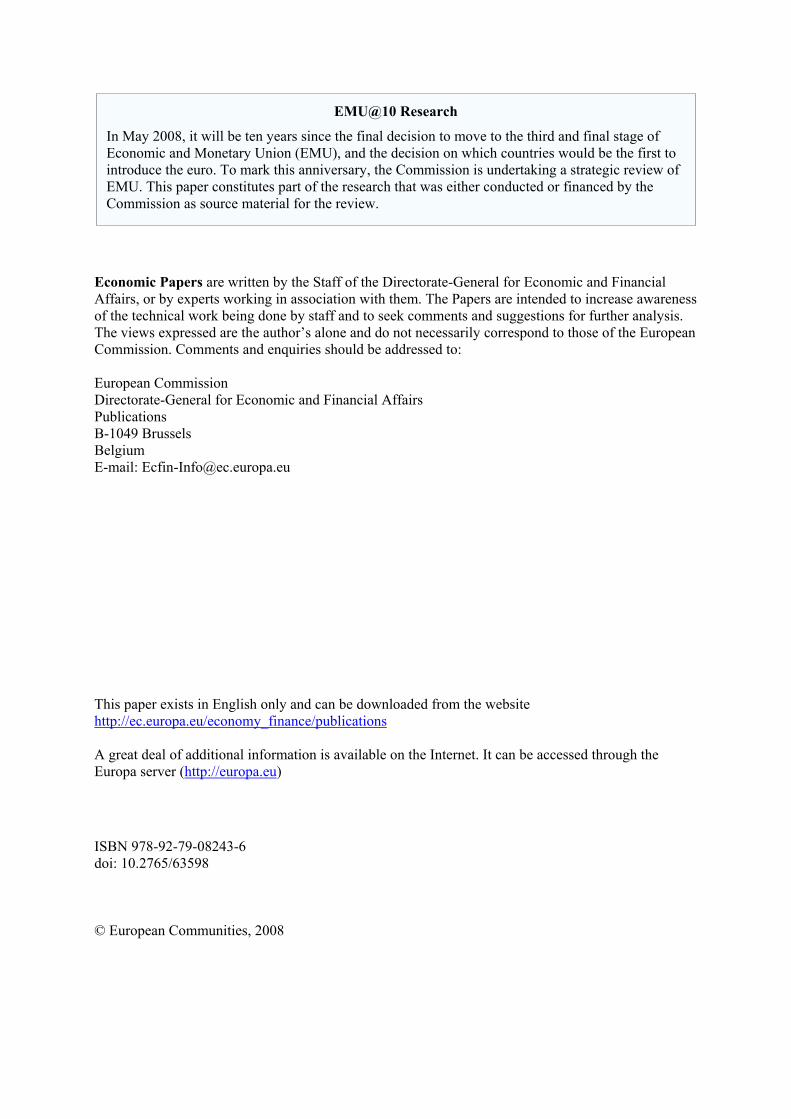
Figure II.4 presents a comparison of TFP growth in the Euro Area and the non-EMU EU members. The EU countries outside the Euro Area experienced faster TFP growth as compared to the Euro Area members well in advance of the introduction of the common currency. TFP growth in EMU slowed after the introduction of the euro
Figure II.5 illustrates the calculations for TFP growth on a country-by-country basis7. TFP growth slowed between 1997-2001 and 2002-2006 in almost all EU countries, both inside and outside of EMU. TFP growth was particularly robust in Finland and Ireland8 between 1997 and 2001. Productivity growth in the UK and in Sweden was
6 We have assumed that the self employed receive the same wage per hour as the employed. 7 Basic price data are not available for Greece, and we do not present that country separately. In Figure II.4 we have made the appropriate but approximate adjustment to the Greek market price data in order to calculate the aggregate for the Euro Area. 8 The strong growth in Ireland may in part reflect transfer pricing from elsewhere in Europe. In most countries GDP is a good indicator of production and incomes received by domestic residents. Incomes of residents can be scaled by GNP, and as a rule GDP and GNP move together. However, Ireland has been chosen by non-EU firms as a location for declaring profits to ensure that they are remitted at low tax rates. The ratio between GDP and GNP in Ireland was around 1.1 in 1986, and stayed at that level for a decade. When it became clear that Ireland would be in monetary union there was a sharp increase in profits oriented transfer pricing through that country and between 1996 and 1998 the ratio rose by six percentage points. The allocation of profits to Ireland on this scale will have raised measured output and productivity growth in a spurious way. Over this period the equivalent ratios in the UK, the US and Belgium fluctuated around or just below one despite their differing net foreign asset positions.

10
higher in this period than in any of the other Euro Area countries, and it remained so between 2002 and 2006. However, TFP growth was only noticeably lower than in the UK in Italy, Spain and Belgium between 1997 and 2001, and in the same countries along with the Netherlands, Austria and Portugal between 2002 and 2006. In both these periods productivity growth in France and Germany was marginally lower than in the UK. Productivity levels actually declined in Spain in the second two sub periods and in Italy in the last period.
Figure II.5 TFP growth (basic prices)
-1.0%
0.0%
1.0%
2.0%
3.0%
4.0%
5.0%
6.0%
7.0%
8.0%
UK
Swed
en
Den
mar
k
Ger
man
y
Fran
ce
Italy
Spai
n
Net
hs
Belg
ium
Finl
and
Aust
ria
Portu
gal
Irela
nd1992-1996 1997-2001 2002-2006
Some of the factors affecting TFP growth are discussed in Barrell (2007), Crafts (2007) and McMorrow and Röger (2007). We can decompose them into the skills of the workforce, the level of scientific knowledge and the efficiency with which factors of production are used. Any production function may be written as Yt=f(capitalt, labourt, techt) where the labour input is in efficiency units and techt picks up other forms of technical progress. If we cannot measure labour in efficiency units then the tech term will be a combination of labour skills effects and other technology and productivity effects. If we were able to measure labour in efficiency units (rather than in person hours) then the resulting tfp calculated from equation (1) above would
11
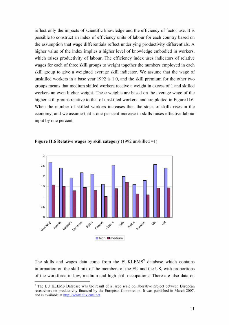
reflect only the impacts of scientific knowledge and the efficiency of factor use. It is possible to construct an index of efficiency units of labour for each country based on the assumption that wage differentials reflect underlying productivity differentials. A higher value of the index implies a higher level of knowledge embodied in workers, which raises productivity of labour. The efficiency index uses indicators of relative wages for each of three skill groups to weight together the numbers employed in each skill group to give a weighted average skill indicator. We assume that the wage of unskilled workers in a base year 1992 is 1.0, and the skill premium for the other two groups means that medium skilled workers receive a weight in excess of 1 and skilled workers an even higher weight. These weights are based on the average wage of the higher skill groups relative to that of unskilled workers, and are plotted in Figure II.6. When the number of skilled workers increases then the stock of skills rises in the economy, and we assume that a one per cent increase in skills raises effective labour input by one percent.
Figure II.6 Relative wages by skill category (1992 unskilled =1)
0
0.5
1
1.5
2
2.5
3
German
y
Austria
Belgium
Denmark
Spain
Finlan
d
France Ita
lyNeth
s
Sweden UK US
high medium
The skills and wages data come from the EUKLEMS9 database which contains information on the skill mix of the members of the EU and the US, with proportions of the workforce in low, medium and high skill occupations. There are also data on 9 The EU KLEMS Database was the result of a large scale collaborative project between European researchers on productivity financed by the European Commission. It was published in March 2007, and is available at http://www.euklems.net.

12
the relative compensation of these groups over time and therefore it is possible to produce a compound skill indicator if we assume that the skill level of the unskilled is constant and that relative wages reflect relative marginal product10. Table II.4 reports average annual growth of a skills index with fixed weights based on 1992 for each of the countries where we have data. Care has to be taken in the interpretation of these data when making cross country comparisons at a single point in time, as definitions of skill categories differ between countries, especially amongst the high skilled groups. Educational systems also differ, with average graduates representing a larger and different group in the US than in most European counties. However, these differences matter less when we make comparisons over time within a country as definitions and education systems change much less in this dimension.
Table II.4 The growth rate of skills
period BG DK FN FR GE IT NL OE SD SP UK US 85-89 0.4 0.5 0.4 0.7 0.4 0.2 0.4 0.5 0.3 0.8 0.7 0.3 90-94 0.8 0.6 0.7 0.8 0.3 0.2 0.3 0.5 0.3 0.8 1.0 0.3 95-99 0.5 0.4 0.2 0.6 0.0 0.2 0.3 0.5 0.2 0.7 0.8 0.3 00-04 0.4 0.3 0.2 0.4 0.2 0.1 0.2 0.3 0.6 0.7 0.6 0.4
Note: BG=Belgium, DK=Denmark, FN=Finland, FR=France, GE=Germany, IT=Italy, NL=Netherlands, OE=Austria, SD=Sweden, SP=Spain. Source: Own calculations using EUKLEMS data
The existence of the skills data constrains both the time frame and the country coverage of this study. They are available from 1980 for most countries, but EUKLEMS data starts later for Sweden, for instance. We have extended the Swedish data back using national sources. In other countries, such as Spain, the growth of skilled and semi skilled occupations has been rapid because of the urbanisation and industrialisation catching up process that country has undergone, and the meaning of the unskilled group may change over time in such situations. Hence caution has to be used when utilising these data. While it is difficult to make cross-country comparisons because definitions of skills vary greatly across countries, it is clear that the relatively slow accumulation of skills in Germany over the past two decades as compared to the UK and France may be one reason for relatively low productivity growth in the Euro Area’s largest economy. The differential accumulation of skills shows up mainly amongst university graduates, and figure II.7 shows their share in total employment.
10 A skills index can be constructed either by using a Tornquist discrete time version of a Divisia index, or it can be constructed with fixed weights. We have experimented with both, and marginally prefer the fixed weight index shown in Table II.4. The chain weighted index induces a cycle into the quality index that is related to the business cycle, as wage differentials become compressed or expand over the business cycle. If we could choose either similar points on the cycle or calculate cycle average relative wages then we could construct an approximate Tornquist index.

13
The proportion of employees with university education has grown faster in the UK and France as compared to Germany over the past several decades.
Figure II.7 Percent of university graduates in total employment
0
5
10
15
20
25
30
35
1980
1982
1984
1986
1988
1990
1992
1994
1996
1998
2000
2002
2004
perc
ent
Germany France UK US
We repeat our growth accounting, taking into account the quality of labour. If St, is the stock of skills then a skills adjusted tfp indicator, denoted tfps, can be written as:
tfps = dlnYt -[btdlnKt + (1-bt) dln(EtHtSt)] (2)
For growth accounting purposes we can use the time period from 1991 for comparison, and if we do that we only lose Greece, Portugal and Ireland from our calculations, as the former has neither the basic price GDP data and skills information we need, whilst the latter two do not have enough information on skills and relative wages to be included in the comparison.
Figure II.8 plots the skills adjusted TFP growth for the Europeans where we have a sufficiently reliable data set, and compares the period before the formation of EMU with that afterwards. After skills adjustment, TFP growth was similar in the UK, Germany and the US over the period 1999-2004.

14
However, in the Euro Area as a whole TFP growth on a skills adjusted basis averaged less than 1 per cent per annum, or about half a percentage point lower than in Germany, the UK and the US11.
Figure II.8 Skills adjusted TFP growth
-1.5%
-1.0%
-0.5%
0.0%
0.5%
1.0%
1.5%
2.0%
2.5%U
K
Sw
eden
Den
mar
k
Ger
man
y
Fran
ce
Italy
Spa
in
Net
hs
Bel
gium
Finl
and
Aus
tria
Ann
ual g
row
th
1993-1998 1999-2004
Figure II.9 Unadjusted TFP growth
-0.5%
0.0%
0.5%
1.0%
1.5%
2.0%
2.5%
3.0%
UK
Sw
eden
Den
mar
k
Ger
man
y
Fran
ce
Italy
Spai
n
Net
hs
Belg
ium
Finl
and
Aus
tria
annu
al g
row
th
1993-1998 1999-2004
11 In order to calculate this figure we have used our factor price adjustment for Greece and we have assumed that skills in Ireland, Portugal and Greece grew at the same rate as in France, a country that performed well. Changes in these assumptions would only marginally change the results as these three countries represent a small share of Euro Area output

15
Figure II.9 reports TFP growth before skills adjustment for the same period and countries. It is clear that TFP growth was particularly low in Spain and Italy, especially during the EMU period, but skills adjusted or not, TFP growth rates, especially in Spain, were also weak before the formation of EMU. TFP growth was positive and accelerated in the EMU period in France, Netherlands, Finland and Austria, and only Italy experienced a marked slowdown of skills adjusted TFP growth into the EMU period.
As with the previous analysis we also lose the US because it lacks data for constant price output at basic prices, although we can approximate this data for the US over the same period. These estimates suggest that TFP growth was around 1.7 per cent per annum between 1993 and 2004, and that skills contributed about 0.2 percentage points per annum of this, leaving underlying TFP growth (tfps above) at around 1.5 per cent a year on average over this period. These figures for TFP growth are lower than those commonly referred to for the US as they reflect whole economy output and whole economy capital stocks as well as whole economy labour input. Most work on the US, including that published by the Bureau of Economic Analysis, reports figures for TFP growth in the non-farm business sector, and hence misses out the more slowly developing government sector and the agricultural sector.
Figure II.10 Skills component of TFP growth
0.0%
0.1%
0.2%
0.3%
0.4%
0.5%
0.6%
0.7%
UK
Sw
eden
Den
mar
k
Ger
man
y
Fran
ce
Italy
Spa
in
Net
hs
Bel
gium
Finl
and
Aus
tria
annu
al g
row
th
1993-1998 1999-2004
Figure II.10 plots the contribution of skills to the growth rate of these countries. The contribution of skills growth in the UK is noticeably greater than that in Germany or Italy, as we might expect from Table II.4, but the contribution of skills growth was
16
also quite noticeable in France, Spain, Belgium and Austria. These results suggest that most of the poor productivity performance of the German economy in the EMU period has been due to slow skills growth, and to a lesser extent the same is true of France. A low contribution from skills has also been important in Italy, but there are also other factors holding back productivity growth there, as there are in Spain. Productivity growth after factoring out skills has been particularly strong in Sweden and Finland. It would appear that differences in skills growth have contributed about a quarter of a point to the Euro Area growth deficit against the UK since 1999, and around a fifth of a percentage point in the period in the run up to the formation of EMU. Skills growth rates were similar in aggregate to the US12.
Our skills adjusted TFP growth can result from either increases in the stock of knowledge or changes in the competitive environment that make factor use more efficient. All of the European countries were members of the European Union, and hence all will have been influenced by the Single Market Programme, and the only major market efficiency related initiative that separates them is the EMU process. Knowledge comes from many sources, and that part not embodied in the skills of the workforce depends on access to the knowledge base associated with scientific activity. In practice, the stock of knowledge in an economy is often proxied by the levels of Research and Development (R&D) activity and access to technology from abroad through imports and Foreign Direct Investment (FDI).
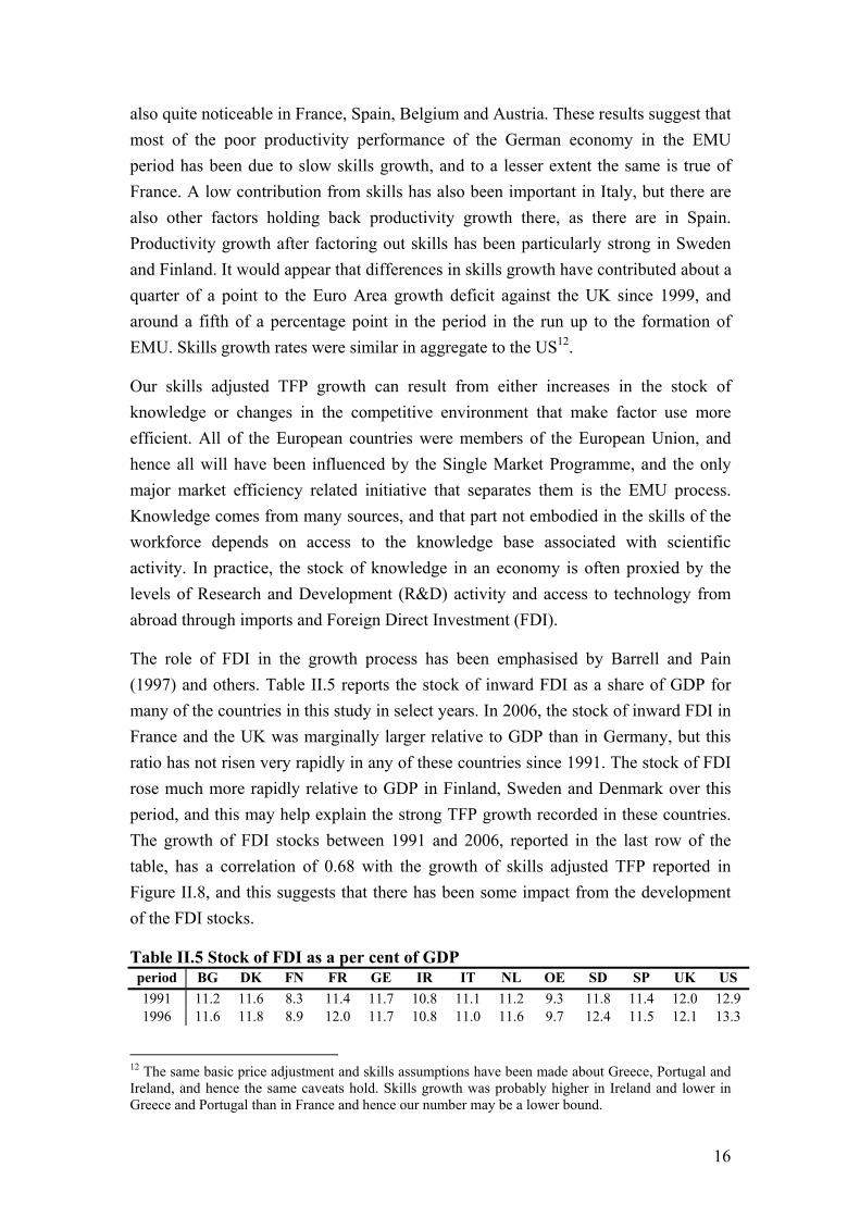
The role of FDI in the growth process has been emphasised by Barrell and Pain (1997) and others. Table II.5 reports the stock of inward FDI as a share of GDP for many of the countries in this study in select years. In 2006, the stock of inward FDI in France and the UK was marginally larger relative to GDP than in Germany, but this ratio has not risen very rapidly in any of these countries since 1991. The stock of FDI rose much more rapidly relative to GDP in Finland, Sweden and Denmark over this period, and this may help explain the strong TFP growth recorded in these countries. The growth of FDI stocks between 1991 and 2006, reported in the last row of the table, has a correlation of 0.68 with the growth of skills adjusted TFP reported in Figure II.8, and this suggests that there has been some impact from the development of the FDI stocks.
Table II.5 Stock of FDI as a per cent of GDP period BG DK FN FR GE IR IT NL OE SD SP UK US 1991 11.2 11.6 8.3 11.4 11.7 10.8 11.1 11.2 9.3 11.8 11.4 12.0 12.9 1996 11.6 11.8 8.9 12.0 11.7 10.8 11.0 11.6 9.7 12.4 11.5 12.1 13.3
12 The same basic price adjustment and skills assumptions have been made about Greece, Portugal and Ireland, and hence the same caveats hold. Skills growth was probably higher in Ireland and lower in Greece and Portugal than in France and hence our number may be a lower bound.

17
2001 12.4 13.3 10.2 12.7 12.6 12.0 11.7 12.6 10.5 13.7 12.2 12.8 14.1 2006 13.0 13.5 10.8 13.2 12.8 11.8 12.2 12.6 10.9 14.2 12.5 13.3 14.4
2006-1991
1.8
1.9
2.5
1.8
1.1
1.0
1.1
1.4
1.6
2.4
1.1
1.3
1.5
Note: BG=Belgium, DK=Denmark, FN=Finland, FR=France, GE=Germany, IR=Ireland, IT=Italy, NL=Netherlands, OE=Austria, SD=Sweden, SP=Spain. Source: UNCTAD and NIESR calculations
A number of endogenous growth models have been developed where R&D expenditures or the number of researchers drive the growth process with Aghion and Howitt (1998) and Griffith et al (2004) being amongst the most significant for our purposes. Not only does R&D increase the innovation rate in the technology frontier country, but it also raises the absorptive capacity of an economy to new ideas. Hence we use an estimate of the stock of R&D at t as an indicator of usable knowledge, based on the accumulation of flows of R&D onto a depreciating stock13.
Table II.6 Stock of R&D – annual average growth rate
period BG DK FN FR GE IT NL OE SD SP UK US 90-94 4.6 5.0 6.9 3.7 3.8 4.0 2.5 6.2 4.9 9.3 1.5 2.8 95-99 4.5 5.6 7.6 2.6 2.9 2.3 2.7 6.1 5.2 6.1 1.3 3.0 00-05 4.0 5.8 7.7 2.4 3.0 2.6 2.1 6.3 5.2 6.8 1.6 3.2
Note: BG=Belgium, DK=Denmark, FN=Finland, FR=France, GE=Germany, IT=Italy, NL=Netherlands, OE=Austria, SD=Sweden, SP=Spain. GERD stock, million national currencies, constant prices, 5% depreciation rate
Table II.6 shows the average growth rates of the R&D stock for all the countries in this study. The stock of R&D grew most rapidly in Finland, Spain and Austria over this sample period. Over the last 10 years, the stock of R&D in Germany has risen at about the same rate as in the US, after growing more rapidly in the previous 10-year period. The stock of R&D in France has risen somewhat more slowly than it has in Germany, while the growth of R&D has been particularly slow in the UK. There seems to be no strong pattern from a simple investigation of the table, unlike with FDI, but more careful investigation, and allowance for other factors should help us uncover any possible role for R&D in explaining differences in productivity growth.
Both R&D and FDI are potential variables that might explain differences in growth rates. However, a number of other factors have been affecting productivity growth in these countries. Increased openness is often regarded as a factor driving growth, and all have become more open over time, at least as measured by the ratio of the volumes of exports and imports of goods and services to output. Openness increases in part 13 We benchmark the stock in 1974, before the beginning of our data period, as the flow divided by the average growth rate and the depreciation rate, and we cumulate flows onto this stock with a depreciation rate of 5 per cent per annum in line with Coe and Helpman (1995). The data comes from the OECD Science and Technology database.

18
because the nature of goods changes, and they become lighter and more mobile, and import penetration rises. However, it is not clear that such changes increase competition and the efficiency of factor use. Openness can also increase because barriers to trade are removed, as with the European Single Market, the North American Free Trade Agreements and other measures that are designed to increase trade and competition. We include indicators of these agreements in our work.
III. The impact of the euro on European economies The introduction of the euro and the conduct of the single monetary policy have helped establish an environment of price stability in the Euro Area. The ECB’s monetary policy has acquired credibility and has succeeded in anchoring long-term inflation expectations to price stability, thereby exerting a moderating influence on price and wage-setting behaviour. To the extent that the introduction of the euro and the implementation of the Single Market Programme removed trade barriers and increased transparency, they may have impacted output and productivity growth directly.
The debate on EMU has centred around three main benefits for the single currency: increased competition and transparency; a reduction of exchange rate volatility and uncertainty within the area; and improved price stability. Increased competition and transparency may improve factor efficiency and raise output for given inputs. It may also reduce the mark-up of prices over costs and raise the equilibrium level of employment. The establishment of the European Monetary Union may have also affected output growth indirectly by for instance reducing the risk associated with output and exchange rate volatility, reducing the cost of investment and encouraging inflows of FDI into and within the region. Identifying and quantifying the impact of EMU on output per person hour adjusted for skills is the subject of the following section. Below we review the existing literature on the impact of EMU on the drivers of potential growth and employment.
3.1 EMU and growth The literature has addressed several aspects of the benefits of EMU and its contribution to economic growth and employment. The economic success or failure of EMU can be judged through its impact on output and employment in the participating countries. Two key factors can be identified through which EMU can be expected to spur growth and employment. One of the most important factors relates to the creation

19
of a macroeconomic policy framework conducive to stability. Another factor concerns the formation of a large single market where prices are denominated in the single currency. The variability of intra-area exchange rates was eliminated with the creation of the euro. In the early part of the 1990s, exchange rate volatility associated with the Exchange Rate Mechanism crisis is thought to have augmented cyclical tensions, leading to recession in the Euro Area.
Although the relatively poor economic performance in the Euro Area over the past several years has received considerable attention, the debate on the culprits of comparatively slow growth and the role of common currency is wide open. The European Commission (2004) suggested that the disappointing Euro Area growth performance in its early years could be viewed as a combination of external shocks to the Euro Area and weak domestic demand growth. They identified three major external developments as having significantly dented economic growth in the Euro Area since the introduction of the single currency. These relate to an oil price hike in 2000, which reduced households’ purchasing power; the pronounced correction of stock market prices starting in the spring of 2000; and most importantly the slump in world trade growth in 2001. However, all these factors affected all OECD countries to varying degrees and therefore cannot explain the slowdown in output growth in the Euro Area relative to the other major economies. In addition, Barrell and Pomerantz (2004) suggest that there is only a small impact of higher oil prices on output growth across many OECD countries. They note that the impact of oil price increases on output depends in part on the oil intensity of production, which has fallen at different rates in different countries in the last two decades, and is generally low in Europe compared to the non-European OECD economies. According to Barrell and Pomerantz (2004) oil price shocks should reduce output marginally in the long run as they change the OECD’s terms of trade and raise the real interest rate. The short run impacts on output can be largely or even completely offset by monetary policy makers, but only at the cost of higher inflation in the short run and higher prices in the long run. Oil prices have continued to rise since the Commission report was published, and growth strengthened in most OECD countries during this period, which supports the suggestion that high oil prices have little impact on output.
Others studies have looked at the role of factor inputs in determining the level of growth. Barrell, Guillemineau and Holland (2007) examine the largest EU economies and argue that Germany has had weak growth in part because labour input has fallen, and this would be difficult to attribute to the introduction of the euro. The United Kingdom’s higher growth has originated mainly from the business and finance sectors, which have benefited from a more rapid diffusion of ICT developments than in other countries, while France’s higher growth relative to Germany since 1999

20
comes essentially from the non-tradable sectors and from a higher labour input. Neither of these developments is thought to be directly related to EMU. Barrell (2007a) suggests that the impact of globalisation and trade agreements may account for the weak growth in Italy. In the short-term to medium-term, it is possible that rising competition associated with trade agreements may have a negative effect on growth in some countries if it necessitates a significant level of restructuring of the economy, and this appears to have been the case in Italy.
Wyplosz (2006) examines the Maastricht convergence criteria, the stability and growth pact and monetary policy strategy. He suggests that the euro has been a major success, but that there have been many secondary problems associated with it. Throughout the 1990s, inflation was cut significantly in the UK, US and ‘Big Four’ Euro Area economies (France, Germany, Italy and Spain). However, whereas GDP growth rose and unemployment fell in both the UK and the US, in the major Euro Area economies GDP growth fell and unemployment remained very high. Wyplosz (2006) suggests that the run up to the introduction of the euro and the one-size-fits-all Maastricht convergence criteria are partly responsible for slow output growth in the Euro Area. He argues that the strong performance of both the US and the UK after 1992 followed from reasons which are unrelated to their location outside the Euro Area. The US had a surge in labour productivity growth in the mid 1990s, driven by ICT investment in the service sector. The rapid decline in equilibrium unemployment in the UK in the 1990s was the underlying factor behind the UK’s superior performance, supported by a decline in unionisation in the private sector and deregulation of the service sector. Hence, Wyplosz argues that the weak macroeconomic performance of the major Euro Area countries since 1999 relative to the UK and the US has little to do with adoption of the single currency.
Lane (2006) discusses how inflation differentials within the Euro Area have been much more persistent as compared to US states. He notes however, that EMU has led to greater economic integration with economic linkages with the rest of the world growing strongly. Lane (2006) also argues that the elimination of exchange rate uncertainty has boosted trade among the member states, which should lead to real convergence between members and in turn higher levels of output growth.
According to Lane (2006) more liquid and deeper financial markets have been created from the emergence of the EMU. Greater financial integration supports economic growth, as it facilitates the capacity to borrow and lend overseas, which enables individual member countries to smooth consumption in the face of temporary shocks to domestic income. It also improves the ability to diversify financial risks, reducing the exposure of domestic wealth to domestic shocks. However, Cappiello et al. (2006)

21
find that whilst the euro has enhanced regional financial integration in the Euro Area in both equity and bond markets, there are some areas, such as the European banking system, in which financial market integration has not yet had a significant effect.
Financial integration is quite broad as it embraces a mixture of financial instruments, a wide array of financial intermediaries, and a variety of financial market segments. Baele et al. (2004) note that the euro has had a visible impact in the reorganisation of several segments of European financial markets, such as the money markets. In other segments, the introduction of the euro may be starting to contribute to greater depth and liquidity. Indeed, the scale of the euro denominated corporate bond market has grown rapidly and many equity investors now treat the Euro Area as a single entity. However, there are some effects of financial market integration that may enhance heterogeneities inside the Euro Area in the future. Kalemli-Ozcan et al. (2003) suggest that higher financial integration may lead to more asymmetric macroeconomic fluctuations, with economic integration leading to greater risk-sharing opportunities through financial market integration.
There is little evidence that income levels in the Euro Area have been converging. Indeed, Giannone and Reichlin (2006) show that output levels are not converging in Europe, with the exception of the remarkable catch-up of Ireland’s output. However, they are clearly not diverging either. They suggest that cyclical asymmetries among Euro Area countries are relatively small and similar to those among US regions. They find that the response of the Euro Area to a world shock lags the US and its cycle is more persistent, but less volatile. Giannone and Reichlin (2006) show that common shocks account for the bulk of output fluctuations in the Euro member states. Country specific shocks have small but persistent effects, and these, rather than heterogeneous responses to common shocks, are the main culprits for existing asymmetries among Euro Area countries.
3.2 EMU and openness Over the last three decades, the reduction of trade barriers to the movement of goods and services and of capital has fostered rapid growth of trade relative to output. Even taking into account rapid trade growth in the post WWII period, the 1990s stand out as particularly robust. This decade was characterised by a deepening of regional integration, via regional trade agreements such as the North American Free Trade Agreement (NAFTA), the completion of the European Single Market (SMP) and the formation of the World Trade Organisation (WTO). Barrell, Liadze and Pomerantz (2007) show that these trade liberalising initiatives can account for much of the strong growth in trade observed in the 1990s, while Barrell (2007a) suggests that stability

22
within the Euro Area has been helped by overall stability throughout the world economy through increased openness and liberalisation of trade and financial markets.
As regards the European Monetary Union, there is a large body of empirical evidence suggesting that currency unions have a substantial positive impact on trade volumes between members. Rose (2000) used a gravity equation approach to assess the separate effects of exchange rate volatility and currency unions on international trade. The panel data set used includes bilateral observations for five years spanning 1970 through 1990 for 186 countries. In this data set, there are over one hundred pairings and three hundred observations, in which both countries use the same currency. He examines their openness ratios, namely, the sum of trade divided by real GDP and finds a large positive effect of a currency union on international trade, and a small negative effect of exchange rate volatility. These effects are statistically significant and imply that two countries that share the same currency trade three times as much as they would with different currencies.
The Rose (2000) study has been widely criticised due to omitted variables that are pro-trade and correlated with the currency union dummy, model mis-specification and reverse causality in that big bilateral trade flows cause a common currency rather than vice-versa. In addition the majority of his comparisons involved monetary union changing to non union at the time of a break down in a colonial relationship, and hence the impacts on trade may have been caused by the latter not the former. More recent studies focusing on the impacts of the European Monetary Union on trade obtain much less impressive results. Bun and Klaasen (2002) and Micco et al. (2003), for instance, found that EMU increased trade volumes by 15 to 38 per cent within member countries. Baldwin (2006) reassesses the origins, methodology and principal findings of the empirical literature that has looked at currency unions preceding EMU and reviews the specification of the gravity model and estimation strategies. His analysis recalibrates the trade effects of currency unions for non-European cases. Baldwin (2006) suggests that the trade effects are still important but less sizeable than in early estimates by Rose (2000). In his view, the euro has already boosted intra-Euro Area trade by around 5 to 10 per cent on average, although the estimated size of the effect is likely to change as new data becomes available. He notes, however, that given that trade among European countries has continuously risen over the last 50 years, it may indeed be difficult to witness further spectacular surges in intra-European trade.
3.3 Exchange rate volatility and investment The elimination of exchange rate instability and uncertainty has been one of the main benefits attributed to the creation of the single currency. As theory does not have a

23
clear conclusion on the role of uncertainty in the determination of the level of investment, it is an empirical matter. Bagela et al (2004) investigate whether the formation of EMU has reduced exchange rate volatility and hence raised growth. Although they do not find direct effects of exchange rate volatility on growth in the Euro Area, they do uncover it is a larger group of countries. As they show EMU has reduced exchange rate volatility they conclude it has had a weak but positive effect on growth.
Evidence on the impacts of exchange rate and other forms of uncertainty on investment has accumulated only slowly, in part because it is difficult to measure anticipated or expected volatility, as it is important to distinguish between components of volatility and hence find their effects. Broadly, it is agreed that increased uncertainty reduces investment (Carruth et al., 2000) but in some cases firms could increase investment but reduce output to cover risks. In general we would expect that increased uncertainty would reduce the level of output.
The most interesting studies on the relationship between volatility and investment tend to look at several countries and several potential indicators of risk. Darby et al. (1999) found evidence that exchange rate uncertainty can have significant negative long-run effects on investment. They find that exchange rate stability increases investment in Europe on average, although the benefits are concentrated in France and Germany, whereas Italy and the United Kingdom do not reap any permanent gains, although these differences were not subject to significance tests.
Byrne and Davis (2005a) used Pooled Mean Group (PMG) panel data studies to look at the factors affecting investment in order to address the role of risk in investment. Conditional GARCH measures were used to isolate the predictable components of uncertainty to estimate their effects on Business Sector data on investment in the US, Japan, Germany, France, Italy, the UK and Canada. The authors looked at uncertainty as measured by conditional volatility of monthly CPI, long rates, effective nominal and real exchange rates, industrial production and equities; the authors found that only nominal and real exchange rate uncertainty have important negative impacts on investment for the whole sample, and exchange rate uncertainty effects appear to increase over time. There is also evidence that long term interest rate uncertainty matters in Europe, although the evidence is not robust. In a related paper Byrne and Davis (2005b) examined the relationship between aggregate investment and nominal effective exchange rate uncertainty in the G7, using panel estimation and a decomposition of volatility into the short and long run components derived from a Components GARCH model. They found that for a poolable subsample of European

24
countries, it is the transitory and not the permanent component of volatility which adversely affects investment.
3.4 EMU and FDI The incipient empirical research on the direct impacts of the EU and EMU on foreign direct investment has shown that European integration has helped stimulate trade and cross-border investment within the EEA (Dunning 1997, Barrell and Pain 1999 and Pain and Young 2003). In particular, US investment to the UK, Ireland, Spain and Sweden is shown in Barrell and Pain (1998) to be sensitive to membership of the EU. Barrell and Pain (1997) find that technology transfer through FDI has affected the rate of technical progress within the German and UK economies. This suggests that to the extent that EMU can be shown to have a positive impact on inward FDI, it may increase output growth by affecting the rate of technological progress.
In a gravity model based study of bilateral FDI flows Petroulas (2007) found that EMU increases inward FDI flows within the Euro Area by approximately 16 per cent, outward FDI from member countries to non-members by approximately 11 per cent, and a weak increase in inward FDI from non-member countries to the Euro Area of around 8 per cent. He also examines whether the introduction of the euro has increased the concentration of FDI in some member countries in detriment to others. He found evidence that FDI flows tend to concentrate in large countries –measured by market size- whilst exports tend to increase more for small countries. However, the author notes that these results are not robust and should be investigated further. Indeed, these findings contrast with those of Ricci (1998), where it is shown that small countries receive less FDI when exchange rate volatility is higher.
Most of the literature on the single currency and FDI has focused on the potential to reduce exchange rate instability and uncertainty, and as a result increase foreign direct investment. However, in sharp contrast with the research on currency union and trade, the evidence regarding the impacts of exchange rate uncertainty on FDI is ambiguous. Although theoretical and empirical studies find clear evidence that the level and volatility- which proxies uncertainty- of exchange rates can have a significant impact on FDI, it is much less clear whether the impact is negative or positive because it depends on whether the FDI is designed to serve the host market or the home (or other) market. In the former case exchange rate volatility may raise FDI to reduce risk, whilst in the latter exchange rate volatility may reduce FDI to reduce risk. Some papers on FDI and exchange rate volatility were based on a theoretical framework developed for the analysis of investment. For instance, Cushman (1985, 1988), Bénassy-Quéré, Fontagné and Larèche-Révil (2001), and Barrell, Gottschalk and Hall (2007), adopt a portfolio analysis approach to the determinants of FDI and exchange

25
rate uncertainty. Cushman (1985, 1988) find evidence that volatility increases US bilateral FDI to Canada, France, Germany, Japan, and the UK, and Goldberg and Kolstad (1995) find analogous results for US FDI to Canada, Japan and the UK. Chakrabarti and Scholnick (2002) find a negative relationship between US outward FDI to 20 OECD countries and exchange rate volatility, while Görg and Wakelin (2002) find negligible exchange rate volatility effects in a sample of US FDI to 12 OECD countries. Ricci (1998) also finds a negative relationship between exchange rate volatility and net OECD FDI to small countries, but a positive relationship when large countries are considered. Sekkat and Galgau (2001) and Zhang (2001) investigate intra-EU and non-EU FDI flows and both conclude that increased exchange rate volatility is likely to raise intra-EU investment flows. Sekkat and Galgau (2001), however, find that non-EU FDI may be deterred by bilateral exchange rate volatility.
The issues of exchange rate regime and the location of inward FDI are particularly important in the European Union. Many FDI decisions are made by firms looking for an export base from which to serve a wider supranational market. In this case, the potential degree of volatility between the currencies of the host and that of the final market will also matter for the investment decision. Barrell, Gottschalk and Hall. (2007) examine how the location decision of US FDI between the UK and mainland Europe would be affected by the volatility and the co-movement of the euro and the pound relative to the dollar. According to Cushman (1985), the correlation of exchange rates matters when multinational firms try to reduce the overall risk of their foreign investment by producing in multiple locations. If exchange rates become increasingly correlated, the risk diversification motivation for investment is reduced, and other determinants of investment will predominate. Barrell Gottschalk and Hall (2007) find that a convergence of exchange rate movements would result in the UK gaining additional FDI by joining the Euro Area
3.5 EMU and labour markets Since membership of the single currency eliminates exchange rate uncertainty, other factors influence FDI decisions. Barrell and Pain (1996, 1997, 1998) found that market size and relative unit labour costs in the manufacturing sector are important determinants of US and Japanese outward FDI to Europe. Econometric results in Barrell and Pain (1998) show that an increase of 1 per cent in costs in one host location relative to the costs in another potential host would decrease the stock of US FDI to Europe by 0.75 per cent. Delbecque and Larèche-Révil (2007) found analogous results in an econometric analysis of the location decisions of European firms within the European Union. However, their analysis emphasizes how labour

26
market regulations and institutions influence FDI decisions. In particular, they examine the impacts of hiring and firing costs, employment protection legislation, trade union membership density and collective bargaining on FDI flows. Their results show that an increase in hiring and firing costs and in employment protection increases labour costs and thus tend to depress foreign investment. Widespread trade union membership has similar negative impacts on FDI, whilst collective bargaining tends to increase inward FDI.
Structural reforms in labour and product markets are desirable in a number of Euro Area countries to improve economic performance. In reality, however, they have proved difficult to undertake. A key issue is whether belonging to the Euro Area affects the political economy of reform in the direction of either helping or hindering structural reform. Duval and Elmeskov (2006) empirically examine the political economy of structural reforms, and investigate whether EMU is encouraging or hindering product and labour market reforms. This is an issue that is much debated in the literature although no consensus view in this respect has emerged as yet. Bertola and Boeri (2002) take stock of reforms carried out in Europe in the field of employment protection and unemployment benefits. Their data point to an acceleration since the mid 1990s episodes of reforms, especially in the Euro Area and in the field of unemployment benefits. This finding would be consistent with the argument put forward by Blanchard and Giavazzi (2003), who claim that product market deregulation and enhanced competition would decrease total rents to be shared and, with them, the incentives for workers to appropriate such rents. That in turn would weaken labour unions bargaining position, reducing insider power and would thus lead to labour market deregulation.
Using OECD databases on labour market reform and product market legislation, Duval and Elmeskov (2006) observe that on average, the intensity of structural reforms between 1994 and 2004 has been greater in the Euro Area than in the rest of the OECD, with top reforming countries being small EMU countries. They note that reforms have also been far reaching while at the same time more comprehensive in the Euro Area than other OECD countries over the past decade. They find evidence that large countries participating in exchange rate arrangements which constrain their monetary policy autonomy tend to undertake fewer reforms than other countries. This is consistent with larger countries having a greater need for monetary accommodation of structural reform whereas for small, open economies such accommodation to a larger extent occurs spontaneously via endogenous changes in competitiveness and external trade. In addition, there appears to have been a slowdown in the reform process in EMU countries after the formal introduction of the euro. Furthermore, comparison of reform progress across policy areas shows that EMU countries have

27
not generally made more progress in reforming the difficult areas, where political resistance is usually strong, than other OECD countries.
Nickell (2006) agrees with Duval and Elmeskov (2006) that the EMU may reduce the incentives to undertake structural reforms of labour and product markets. The difficulty may be more pronounced for a large economy where the response of output to the lowering of inflation and hence to the improved competitiveness resulting from reforms may tend to be slower than in smaller and open economies. Nickell (2006) notes that the rise in potential output will translate only gradually into an increase in actual output and employment.
Holland (2007) develops the Layard, Nickell and Jackman (2006) framework where equilibrium unemployment follows on from the wage bargain and price setting. They assume, reasonably in a European context, that wages are set in bargains between employers and employees and depend in the long run on productivity and labour market institutions. The adjustment of wages to equilibrium depends on the level of excess unemployment, and on expectations of and inertia in response to price changes which also depend on institutions. These institutions help determine the equilibrium level of employment, and labour market reforms will change this equilibrium. It is important to know whether these reforms have been progressed or delayed by the formation of EMU14.
Equilibrium employment depends on the bargaining based wage equation and on the price equation (or factor demands), and there should be a role for competition and liberalisation. Holland (2007) shows that the form of the production function matters, as it affects the relationship between wages and unit costs. The study assumes prices are a mark up over unit cost which depends on the output gap and on competition indicators, such as the European Single Market, the liberalisation of world trade as well as EMU and general openness. The study analyses the mark up in the US, Germany, France, Italy, the UK, the Netherlands, Sweden and Finland. Openness has risen in all these countries, and this may have put downward pressure on margins. However, at the same time more of world trade has been covered by agreements, and hence competition effects may also come for that source.
When Holland (2007) includes the regional and global integration variables in a cointegrating VAR of prices, wages and productivity capacity constraints have a clear role in the mark-up and point to a price elasticity of demand of -0.2. It is also clear that trade liberalisation, both on a global and European scale have reduced mark-ups, and that liberalisation has had a clear effect on the sustainable level of employment in 14 Duval and Elmskov (2006), which includes comments from Nickell, discusses the impact of EMU on reforms, and suggests that it has probably slowed it in the larger economies.
28
European countries, However, it does not appear that the transparency associated with the euro has had a significant impact on the mark-up. At least as importantly, it is clear that openness has a greater impact on technological diffusion than on margins, and has not reduced margins, although it may have increased growth through its impacts on R&D and FDI.
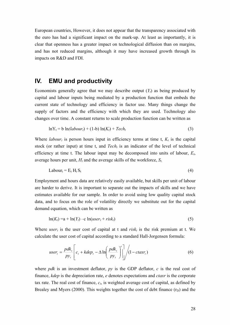
IV. EMU and productivity Economists generally agree that we may describe output (Yt) as being produced by capital and labour inputs being mediated by a production function that embeds the current state of technology and efficiency in factor use. Many things change the supply of factors and the efficiency with which they are used. Technology also changes over time. A constant returns to scale production function can be written as
lnYt = b ln(labourt) + (1-b) ln(Kt) + Techt (3)
Where labourt is person hours input in efficiency terms at time t, Kt is the capital stock (or rather input) at time t, and Techt is an indicator of the level of technical efficiency at time t. The labour input may be decomposed into units of labour, Et, average hours per unit, Ht and the average skills of the workforce, St.
Labourt = Et Ht St (4)
Employment and hours data are relatively easily available, but skills per unit of labour are harder to derive. It is important to separate out the impacts of skills and we have estimates available for our sample. In order to avoid using low quality capital stock data, and to focus on the role of volatility directly we substitute out for the capital demand equation, which can be written as
ln(Kt) =a + ln(Yt) –c ln(usert + riskt) (5)
Where usert is the user cost of capital at t and riskt is the risk premium at t. We calculate the user cost of capital according to a standard Hall-Jorgensen formula:
)1(ln t
e
t
ttt
t
tt ctaxr
pypdk
kdepcpy
pdkuser −
⎥⎥⎦
⎤
⎢⎢⎣
⎡⎟⎟⎠
⎞⎜⎜⎝
⎛Δ−+= (6)
where pdk is an investment deflator, py is the GDP deflator, c is the real cost of finance, kdep is the depreciation rate, e denotes expectations and ctaxr is the corporate tax rate. The real cost of finance, ct, is weighted average cost of capital, as defined by Brealey and Myers (2000). This weights together the cost of debt finance (rD) and the

29
cost of equity finance (rE). The weights are given by the share of capital in the economy that is listed on the stock market. The cost of debt finance is adjusted by the corporate tax rate, reflecting the tax deductibility of borrowing, and is calculated as the risk-free long real interest rate, plus a measure of corporate spreads. Corporate spreads are calculated as the absolute difference between average corporate bond yields and yields on 10-year government bonds15. The cost of equity finance is calculated as the return on equity, which is estimated using price-earnings ratios for a national stock index. While this measure embeds a risk premium into it, our framework allows us to test for the impact of additional risk factors that are not priced into corporate spreads or the return on equity, which do not fully capture expectations.
Substituting our capital equation into our output equation and collecting terms we get
lnYt = γ1 + ln(labourt) – γ2 ln(usert +riskt) + γ3 Techt (7)
where γ3=1/b, γ2 = γ3 *c*(1-b) and γ1 = a*(1-b)*γ3. We are interested in explaining output per person hour after factoring out skills, which we assume has a unit elasticity with respect to labour productivity. This is consistent with the construction of the skills data, where relative wages and relative productivity of the skill groups are assumed to remain constant over time. We may rewrite the equation again by taking Et Ht and St to the left hand side as
ln(Yt / (Et Ht St)) = γ1– γ2 ln(usert + riskt) + γ3 Techt (8)
Output per person hour, after adjusting for skills should in the long run be driven by the user cost of capital, the risk associated with investment and a remaining element we describe as technology, but which covers both the general stock of knowledge, the ability to utilise this stock and the efficiency with which factors of production are organised in utilising this stock of knowledge. The factors that impact on the efficiency of factor use may include the openness of the economy, the competitive environment that is constructed through institutions such as laws, regulations and monetary structures and also social institutions. It is possible that EMU would affect this relationship directly through the competitiveness channel, as it may increase transparency and reduce transactions costs even as compared to having a fixed exchange rate with major trading partners. If we are find the effects of EMU on output growth we must factor out all the other dimension of knowledge and efficiency effects that have been at work in the last decade or so.
15 These data are available for the Euro Area, US, UK, and Denmark. Sweden is assumed to follow the corporate spreads for Denmark. Prior to 1984, the UK spread is assumed to move in line with the US, prior to 1994 the spread for Denmark is assumed to move in line with the US and UK average, and prior to 1999 Euro Area spreads is assumed to move in line with a proxy measure for Germany.
30
There are a number of indicators of knowledge and of the competitive environment that we can utilise. The most obvious are the stocks of Research and Development (R&D) and Foreign Direct Investment (FDI) that we have discussed above, as these either reflect the creation of knowledge or are channels through which it is absorbed. Openness to trade and investment are also thought to have important effects on productivity growth both through knowledge transfers and their efficiency effects. The ability to trade enables a country to specialise in more efficient production processes raising the aggregate growth rate temporarily. Endogenous growth models have also pointed to the possibility that contacts with the outside world may potentially raise the growth rate permanently (see, for instance, Coe and Helpman, 1995; and Proudman ands Redding, 1998). There is also evidence that increases in competition brought about by the intentional removal of barriers to trade and investment raise output, and there is a significant literature, discussed in Badinger (2007), on the impacts of the European Single Market Programme (SMP) on productivity. Membership of the European Union may also have increased productivity by widening the span of competition. There has also been a significant amount of research on the effect of North American Free Trade Agreements (NAFTAs), much of which is summarised in the symposium edited by Lederman and Serven (2005).
We look at these factors in our countries, following Barrell, Liadze and Pomerantz (2007) in the construction of our openness and globalisation indicators. The single market programme (SMP) is a variable that starts in the second quarter of 1987 at 0 and rises to 1.0 in 199216. Not all countries were members at the time, and we index the impact of integration using a dummy that increases over the three years until they become full members, and we denote it as EU. In a similar way we also separately distinguish the impacts of the Canada US Free Trade Agreement in the 1980s and the subsequent wider NAFTA agreement. In order to pick up other trade and competitiveness related factors we have also experimented with openness indicators and have included a measure based on exports plus imports of goods and services divided by GDP (OPEN) in our work. This is the variable that would change if EMU
16 For a detailed description of the Single Market Programme see European Parliament (2008). The Single European Act (which was signed in February 1986 and came into force on 1 July 1987) was a revision of the Treaty of Rome. Its first objective was the incorporation of the specific concept of the internal market in the Treaty defining it as ‘an area without internal frontiers in which the free movement of goods, persons, services and capital is ensured’ and setting a precise deadline for its completion: 31 December 1992. It also wanted to give the completed internal market effective decision-making machinery, by introducing qualified majority voting for most subjects concerned, instead of the unanimity that had hitherto been required. By the deadline, most of the 1992 targets had been met. Over 90 % of the legislative projects listed in the 1985 White Paper had been adopted, largely by using the majority rule. They included full liberalisation of capital movements and total abolition of checks on goods at internal frontiers.

31
had an impact on trade, as the work surveyed by Baldwin (2006) suggests it does, but we factor it out separately as well.
If we wish to investigate the impact of Monetary Union after factoring our other influences on productivity we must include countries who are not members. To that end we include members of the Euro Area along with UK, Sweden, Denmark, and the US in order to compare effects between the two groups. Our country choice and timeframe depend on data, and we are in particular constrained by the availability of skills data over long periods, and in the EUKLEMS database skills stop at 2004. Our end date allows us to use simple volatility indicators for risk, based on the work of Blanchard and Simon (2001).
In our work below we look for the effects of two possible sources of uncertainty for exchange rate volatility and output volatility. In this section we look for a role for the conditional volatility of output, which can be taken as an imperfect indicator or expected volatility. The volatility of output is gauged by the Root Mean Squared Deviations (RMSD) of output around a centred 17 quarter moving average trend. The centred average on which volatility is conditioned uses output data up until the first quarter of 2007 to produce a centred estimate of trend output for the last quarter of 2004, which is the end of our sample period. In the next section we use GARCH techniques to condition the volatility of real exchange rates, which we would expect to influence the equilibrium capital stock. We also test for the effect of real exchange rate volatility in this section by constructing a conditional measure that is equivalent to our output volatility measure. We use a 13 period centred moving average of real exchange rates as the conditional trend and create the RMSD series for this variable17. In both cases these are constructed regressors that give an indication of the variable of interest and as such they are generated regressors that need to be instrumented, as is stressed in Pagan (1984). As these are variables measured with error that we expect to be closely correlated to the true variable of interest we use Durbin’s (1954) method of dealing with errors in variables problems.
It is necessary to find a cointegrating set of variables for each country and then use them to undertake dynamic panel analysis on the dependent variable, output per person hour adjusted for skills (SY). We search across a range of possible sets of driving factors after testing their order of integration, and look for the smallest cointegrating set in each country whilst making sure that the contents remain as similar as possible in order that we may undertake panel analysis. If a variable is included in a cointegrating set when it is not needed that set is not irreducible in the
17 The centered window length was chosen in relation to the cyclical properties of the data.

32
terms of Davidson (1998) and hence we may gain spurious information about the determinants of long run behaviour.
Indicators of increased competition must be included in our cointegrating set as it may increase efficiency and raise output for given inputs. Removal of trade barriers and increases in the scope of markets such as the Single Market Programme, EU entry and North American Trade Agreements are therefore included in cointegrating sets. As a common currency may increase transparency and the effective scope of competition we include an EMU dummy in these sets18.
As we wish to look for direct effects from volatility we separate out the effects of user and volatility. We separate out the effects of ln(user+risk) by noting that ln(a+b) = ln(a*(1+b/a)) = ln(a) +ln(1+b/a). Our basic cointegrating regression is of the form
ittiitititiiti
ititiitiitiiit
NAFTAdEUdEMUdESMdFDIcuservolYcusercDRccSY
ε++++++++++=
43214
3210
)ln())/1ln()ln()&ln()ln(
(7)
but other variables will have been investigated, as we discuss below.
Table IV.1. Unit root test results
level difference level difference levellevel
(including trend)
level difference
Prob. Prob. Prob. Prob. Prob. Prob. Prob. Prob.Austria 0.513 0.003 0.604 0.002 0.140 0.001 0.067 0.000Belgium 0.494 0.000 0.553 0.000 0.000 - 0.465 0.007Denmark 0.797 0.000 0.107 0.000 0.417 0.051 0.080 0.000Finland 0.815 0.000 0.788 0.000 0.094 0.002 0.355 0.000France 0.498 0.000 0.659 0.000 0.005 - 0.373 0.001Germany 0.577 0.001 0.284 0.006 0.001 - 0.225 0.003Italy 0.121 0.008 0.675 0.001 0.000 - 0.260 0.002Netherlands 0.423 0.000 0.425 0.000 0.022 - 0.021 -Sweden 1.000 0.000 0.277 0.000 0.024 - 0.220 0.001UK 0.883 0.000 0.095 0.009 0.552 0.001 0.239 0.003US 0.997 0.000 0.594 0.001 0.334 0.030 0.095 0.011
ln (1+(risk/user cost))ln (dependent variable) ln (user cost) ln (R&D)
Data period 1980q1 2004q4.
We check data for stationarity by testing for the presence of a unit root. Augmented Dickey-Fuller (ADF) tests are computed with an intercept and a lag length of 4 with quarterly data. Test results are reported in table IV 1. Unit root tests indicate that at 5 percent significance level the null hypothesis for the presence of a unit root cannot be 18 The indicators we use are not stochastic regressors, but rather intercept shifts, and hence do not need to be included in the choice of significance levels.

33
rejected for three out of four variables reported. The stock of R&D data has a clear trend over the sample period and it is checked for the trend stationarity. It can be seen from the table that we cannot reject the hypothesis of trend stationarity in R&D series. A hypothesis of unit root is rejected when ADF tests are applied to the first differences of natural logarithms of remaining three variables. We conclude that the dependent variable, the user cost of capital and one plus volatility of output (from now on referred to as risk) over user cost of capital variables are I (1).
Not all variables are needed in the cointegrating set and in particular we find that openness does not need to be in it, despite the popular debate on the role of EMU in increasing trade. Hence we do not report its order of integration, but find that the logged first difference is I(0). Both stocks of Research and Development (R&D) and Foreign Direct Investment (FDI) may drive the efficiency of factor use, but we report only on R&D as it is the preferred variable in all countries except the UK.
It is necessary to check under what conditions can there be a cointegrating set of variables in the long run. We augment the long run equation with dummies for trade such as SMP, NAFTA and EMU and check for the presence of a long run structure. The residuals from the estimated equations are tested for the existence of a unit root, using t-statistics of Augmented Dickey-Fuller tests by including intercept and 4 lags. The results of the cointegration test for the final set of long run equations are presented in Table IV.2. All countries pass the cointegration test.
Table IV.2. Cointegration of the long run t-statistics from the ADF tests for the long run equation
Austria Belgium Denmark Finland France Germany Italy Netherlands Sweden UK US-4.27 -3.83 -3.98 -4.45 -4.86 -4.04 -4.61 -4.31 -3.93 -4.47 -6.20
Data period 1980q1 2004q4. The appropriate critical values are -3.811, -4.100, -4.649 at the 10%, 5% and 1% level.
In our final cointegrating set we have tested for the effects of openness (defined as a sum of exports and imports as a share of GDP) and stock of FDI separately for each country. Adding either openness or FDI raises the critical value for the test but does not raise the test value and as a result not all of the countries pass long run cointegration tests at 5% critical value if they are present. We did not find a systematic role for the openness or FDI in the long run specification for our list of countries with the exception of the UK where FDI was necessary for the existence of the long run relationship. If we include R&D in the UK equation, but do not include FDI, we do not find cointegration. If we remove R&D from the set including FDI we still find that it cointegrates, and hence the irreducible set for the UK include FDI but

34
excludes R&D. Openness was not required for cointegration, but the trade and competition related variables SMP and NAFTA variables were and they may have driven openness. We return to this issue later.
The level of output responds slowly to its determinants, and hence we specify the equation in equilibrium correction form. This allows the effects of all the driving factors such as the SMP, EMU and volatility effects to come through gradually. The dynamic equation can be described by:
dln(Yit / (Eit Hit Sit)) = αi + λi [ln(Yit-1 / (Eit-1 Hit-1 Sit-1)) – βi1 ln(R&Dit-1)
– βi2 ln(userit-1) – βi3 ln(1+(vol(Yit-1)/userit-1) (8) – βi4 ln(FDIit-1) – βi5 SMPt-1 – βi6 EMUt-1 – βi7EUit-1
– βi8 NAFTAt-1)] + γi1dln(Yit-1 / (Eit-1 Hit-1 Sit-1)) + εit
A panel of 11 countries was constructed and estimated by three stage least squares (3SLS). Three stage least squares was used because the volatility of output is a generated regressor measured with an error and we need to instrument it in order to get consistent estimator19. We apply Pooled Mean Group (PMG) estimation method as in Pesaran and Smith (1995) to test for common long run coefficients while allowing for country specific dynamics. Table IV.3 reports the results from the tests on the coefficient commonality in our panel. We start by checking whether common user cost of capital and common (one plus ratio of risk over user cost of capital) can be imposed across countries. Wald tests for commonalities for both variables cannot be rejected. Common SMP effects were found in Belgium, Denmark, France, Germany, Italy and Netherlands and we can impose common EMU effect as well in the same set of countries (except for the Denmark). Table IV 3. Wald test results on commonality
Probability
Common user cost 0.602
Common SMP 0.061
Common EMU 0.486
Common 1+(vol of output/user cost) 0.952
19 We use rank order as an instrument as suggested by Durbin (1954)
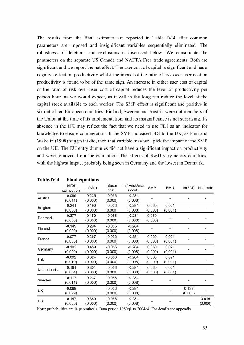
35
The results from the final estimates are reported in Table IV.4 after common parameters are imposed and insignificant variables sequentially eliminated. The robustness of deletions and exclusions is discussed below. We consolidate the parameters on the separate US Canada and NAFTA Free trade agreements. Both are significant and we report the net effect. The user cost of capital is significant and has a negative effect on productivity whilst the impact of the ratio of risk over user cost on productivity is found to be of the same sign. An increase in either user cost of capital or the ratio of risk over user cost of capital reduces the level of productivity per person hour, as we would expect, as it will in the long run reduce the level of the capital stock available to each worker. The SMP effect is significant and positive in six out of ten European countries. Finland, Sweden and Austria were not members of the Union at the time of its implementation, and its insignificance is not surprising. Its absence in the UK may reflect the fact that we need to use FDI as an indicator for knowledge to ensure cointegration. If the SMP increased FDI to the UK, as Pain and Wakelin (1998) suggest it did, then that variable may well pick the impact of the SMP on the UK. The EU entry dummies did not have a significant impact on productivity and were removed from the estimation. The effects of R&D vary across countries, with the highest impact probably being seen in Germany and the lowest in Denmark.
Table.IV.4 Final equations
error correction ln(r&d) ln(user
cost)ln(1+risk/use
r cost) SMP EMU ln(FDI) Net trade
Austria -0.089 (0.041)
0.235 (0.000)
-0.056 (0.000)
-0.284 (0.008) - - - -
Belgium -0.241 (0.000)
0.190 (0.000)
-0.056 (0.000)
-0.284 (0.008)
0.060 (0.000)
0.021 (0.001) - -
Denmark -0.377 (0.000)
0.150 (0.000)
-0.056 (0.000)
-0.284 (0.008)
0.060 (0.000) - - -
Finland -0.149 (0.009)
0.294 (0.000)
-0.056 (0.000)
-0.284 (0.008) - - - -
France -0.077 (0.005)
0.267 (0.000)
-0.056 (0.000)
-0.284 (0.008)
0.060 (0.000)
0.021 (0.001) - -
Germany -0.102 (0.000)
0.459 (0.000)
-0.056 (0.000)
-0.284 (0.008)
0.060 (0.000)
0.021 (0.001) - -
Italy -0.092 (0.019)
0.324 (0.000)
-0.056 (0.000)
-0.284 (0.008)
0.060 (0.000)
0.021 (0.001) - -
Netherlands -0.161 (0.004)
0.301 (0.000)
-0.056 (0.000)
-0.284 (0.008)
0.060 (0.000)
0.021 (0.001) - -
Sweden -0.117 (0.011)
0.237 (0.000)
-0.056 (0.000)
-0.284 (0.008) - - - -
UK -0.069 (0.029) - -0.056
(0.000)-0.284 (0.008) - - 0.138
(0.000) -
US -0.147 (0.005)
0.380 (0.000)
-0.056 (0.000)
-0.284 (0.008) - - 0.016
(0.000)Note: probabilities are in parenthesis. Data period 1980q1 to 2004q4. For details see appendix.

36
The speed of reaction varies across countries and it is highest in the small open economies, Belgium Denmark, Finland and the Netherlands. France Italy and Germany within the monetary Union, and the UK outside it have slower reactions, with the half life of adjustment probably coming after 5 years. The US adjusts more rapidly than any of the other large economies, despite its size. The EMU effects are positive and significant in the five core countries, and they indicate that over the longer term output may be raised by 2 per cent or so by membership of EMU. We did not find any significant effect of EMU either on other member countries or outsiders. To test the robustness of our conclusions we added back EMU variables into the equations of all countries in the final panel and checked for the significance of the coefficients. The results reported in Table IV.5 show that EMU is insignificant in all but five core countries. There are no clear negative effects of the existence of EMU on those who were outside.
Table.IV.5 Robustness check for EMU effects –adding the dummy back in
Austria Belgium Denmark Finland France Germany Italy Netherlands Sweden UK US-0.013 (0.612)
0.019 (0.004)
-0.007 (0.598)
-0.014 (0.305)
0.019 (0.004)
0.019 (0.004)
0.019 (0.004)
0.019 (0.004)
0.014 (0.513)
0.036 (0.406)
0.006 (0.749)
Note: probabilities are included in parenthesis
Our result that openness and stock of FDI (except for the UK in the case of the latter variable) are not in the cointegrating set as a direct determinant of output needs to be seen to be robust, and we undertook further tests. Openness and stock of FDI separately are added back into the final panel specification as a part of the long run and checked for the significance. As it is demonstrated in Table IV.6 below openness is insignificant in each country (apart from the France) and as a panel variable. The FDI effect reported in Table IV.7 is found be insignificant in most countries as well – the exception is Sweden and again France. It seems that after adding EMU, SMP and NAFTA dummies to our equations there is no direct role left for the either openness or FDI stock, except for the France where the above effects still may be present.
Table. IV.6 Openness effects: adding the variables back in
Austria Belgium Denmark Finland France Germany Italy Netherlands Sweden UK US-0.216 (0.357)
0.032 (0.607)
-0.026 (0.820)
-0.195 (0.073)
0.302 (0.009)
-0.030 (0.715)
-0.760 (0.211)
-0.061 (0.475)
-0.216 (0.557)
0.442 (0.061)
-0.520 (0.464)
Probabilities in brackets

37
Table IV.7 FDI effects: adding the variables back in Austria Belgium Denmark Finland France Germany Italy Netherlands Sweden UK US-0.052 (0.278)
0.027 (0.321)
-0.011 (0.413)
-0.019 (0.177)
0.064 (0.000)
-0.001 (0.974)
-0.021 (0.514)
-0.031 (0.397)
0.040 (0.003) - -0.010
(0.545) Probabilities in brackets In this study two different indicators of volatility are used, with the conditional volatility of output being included in the cointegrating set. We also use the conditional volatility of real exchange rates in the next section, and can test for the robustness of our results if we add this variable or substitute it for the volatility of output. Table IV.8 reports tests where we firstly substitute output volatility in the risk premium term with real exchange rate volatility and secondly where we include real exchange rate volatility along with output volatility in the risk premium variable in our final panel set. As real effective exchange rate volatility is a generated repressor, new instrumental variable is created and used in both cases. We estimate both panels by 3SLS. In the first set, where we substitute the volatility measure, the new variable is not significant. In the second set we add the new variable, and it is also not significant. In addition the coefficients for the user cost and the output volatility measure are little changed. It appears that there is no role for the real exchange rate volatility in our final panel specification.
Table IV.8 Substituting and adding real exchange rate volatility effects
Austria-0.040 (0.000)
-0.015 (0.588) Austria
-0.057 (0.000)
-0.425 (0.000)
0.0656 (0.123)
Belgium-0.040 (0.000)
-0.015 (0.588) Belgium
-0.057 (0.000)
-0.425 (0.000)
0.066 (0.123)
Denmark-0.040 (0.000)
-0.015 (0.588) Denmark
-0.057 (0.000)
-0.425 (0.000)
0.0656 (0.123)
Finland-0.040 (0.000)
-0.015 (0.588) Finland
-0.057 (0.000)
-0.425 (0.000)
0.0656 (0.123)
France-0.040 (0.000)
-0.015 (0.588) France
-0.057 (0.000)
-0.425 (0.000)
0.0656 (0.123)
Germany-0.040 (0.000)
-0.015 (0.588) Germany
-0.057 (0.000)
-0.425 (0.000)
0.0656 (0.123)
Italy-0.040 (0.000)
-0.015 (0.588) Italy
-0.057 (0.000)
-0.425 (0.000)
0.0656 (0.123)
Netherlands-0.040 (0.000)
-0.015 (0.588) Netherlands
-0.057 (0.000)
-0.425 (0.000)
0.0656 (0.123)
Sweden-0.040 (0.000)
-0.015 (0.588) Sweden
-0.057 (0.000)
-0.425 (0.000)
0.0656 (0.123)
UK-0.040 (0.000)
-0.015 (0.588) UK
-0.057 (0.000)
-0.425 (0.000)
0.0656 (0.123)
US-0.040 (0.000)
-0.015 (0.588) US
-0.057 (0.000)
-0.425 (0.000)
0.0656 (0.123)
Our result seem robust to these checks, and we can conclude that EMU effects do appear to be present, and that there is no statistically significant effect from real exchange rate volatility or from openness on its own in this panel of countries. Hence
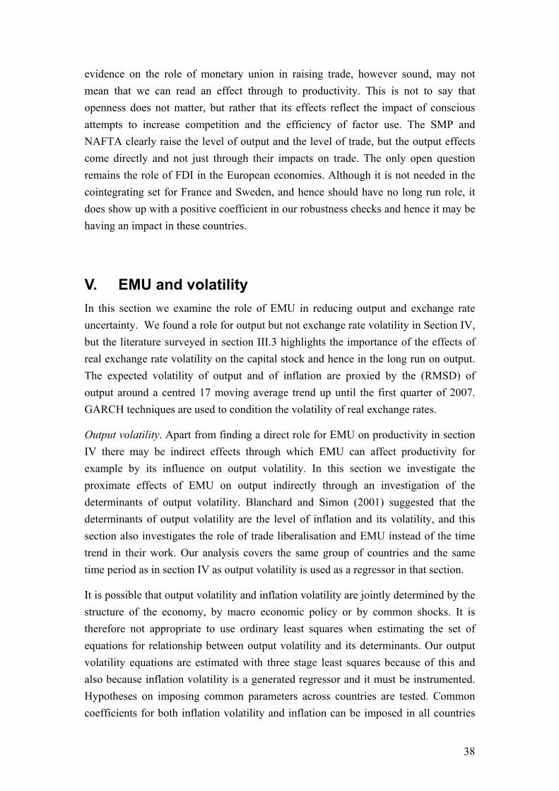
38
evidence on the role of monetary union in raising trade, however sound, may not mean that we can read an effect through to productivity. This is not to say that openness does not matter, but rather that its effects reflect the impact of conscious attempts to increase competition and the efficiency of factor use. The SMP and NAFTA clearly raise the level of output and the level of trade, but the output effects come directly and not just through their impacts on trade. The only open question remains the role of FDI in the European economies. Although it is not needed in the cointegrating set for France and Sweden, and hence should have no long run role, it does show up with a positive coefficient in our robustness checks and hence it may be having an impact in these countries.
V. EMU and volatility In this section we examine the role of EMU in reducing output and exchange rate uncertainty. We found a role for output but not exchange rate volatility in Section IV, but the literature surveyed in section III.3 highlights the importance of the effects of real exchange rate volatility on the capital stock and hence in the long run on output. The expected volatility of output and of inflation are proxied by the (RMSD) of output around a centred 17 moving average trend up until the first quarter of 2007. GARCH techniques are used to condition the volatility of real exchange rates.
Output volatility. Apart from finding a direct role for EMU on productivity in section IV there may be indirect effects through which EMU can affect productivity for example by its influence on output volatility. In this section we investigate the proximate effects of EMU on output indirectly through an investigation of the determinants of output volatility. Blanchard and Simon (2001) suggested that the determinants of output volatility are the level of inflation and its volatility, and this section also investigates the role of trade liberalisation and EMU instead of the time trend in their work. Our analysis covers the same group of countries and the same time period as in section IV as output volatility is used as a regressor in that section.
It is possible that output volatility and inflation volatility are jointly determined by the structure of the economy, by macro economic policy or by common shocks. It is therefore not appropriate to use ordinary least squares when estimating the set of equations for relationship between output volatility and its determinants. Our output volatility equations are estimated with three stage least squares because of this and also because inflation volatility is a generated regressor and it must be instrumented. Hypotheses on imposing common parameters across countries are tested. Common coefficients for both inflation volatility and inflation can be imposed in all countries

39
and Table VI.1 presents results from Wald test for common coefficients across countries and Table VI.2 presents those from the final panel estimation.
Table V.1. Wald test results for commonality
Probability
Common volatility of inflation 0.8743
Common inflation 0.1428
Both inflation and inflation volatility are positively and significantly associated with output volatility in all countries. The EMU effect although small is negative in most countries, which means that it results in the reduction of the volatility of output. The EU membership dummy is significant in Finland and Austria and is negatively related to their output volatility as well. Hence we can claim that there are clear indirect effects of EMU on the level of productivity in the Euro Area though its impacts on the volatility of output and hence on risk premia and investment.
Table V.2. Determinants of output volatility volatility of
inflation inflation emu SMP euentry
Belgium 0.0715 (0.000)
0.0003 (0.000)
-0.003 (0.000)
0.0073 (0.000) -
Denmark 0.0715 (0.000)
0.0003 (0.000)
-0.001 (0.000)
0.0012 (0.028) -
Finland 0.0715 (0.000)
0.0003 (0.000)
-0.002 (0.111)
0.0162 (0.000)
-0.016 (0.000)
France 0.0715 (0.000)
0.0003 (0.000)
-0.003 (0.000)
0.0078 (0.000) -
Germany 0.0715 (0.000)
0.0003 (0.000)
-0.000 (0.373)
0.0009 (0.098) -
Italy 0.0715 (0.000)
0.0003 (0.000)
-0.000 (0.703)
0.0083 (0.000) -
Netherlands 0.0715 (0.000)
0.0003 (0.000)
0.0005 (0.262)
-0.002 (0.000) -
Austria 0.0715 (0.000)
0.0003 (0.000)
0.0019 (0.000)
0.0000 (0.873)
-0.001 (0.004)
Sweden 0.0715 (0.000)
0.0003 (0.000)
-0.001 (0.015)
0.0082 (0.000)
0.0001 (0.830)
UK 0.0715 (0.000)
0.0003 (0.000)
-0.000 (0.332)
-0.001 (0.050) -
US 0.0715 (0.000)
0.0003 (0.000) - - -
Note: probabilities are in parenthesis. Data period 1980q1 to 2004q4. For details see appendix.

40
Exchange rate uncertainty. There has been a growing amount of interest in the relationship between economic uncertainty and its influence on the level of investment recently, and the existing literature is summarised in Section III.3. The conclusion of that literature is that the volatility of the real exchange rate is the one systematic factor that affects the level of investment in cross country panel data analysis. Table V.3 reports average conditional real exchange rate volatility in five year periods for the European countries and the US20. This measure of conditional volatility is the GARCH generated variance of the quarter-on-quarter difference in the (ln of) the real effective exchange rate. In all EMU member countries, with a notable exception of France, real exchange rate volatility has fallen markedly since the introduction of the common currency. This is also true for Denmark and Sweden, neither of whom are members of the Euro Area, but their exchange rates shadow the euro. In contrast, real effective exchange rate volatility increased in the UK, which pursued an independent monetary policy.
Table V.3 Conditional volatility of the real effective exchange rate GARCH estimates, annual average over the period
period BG DK FN FR GE IT NL OE SD SP UK US84-89 0.0151 0.0221 0.0373 0.0285 0.0433 0.0521 0.0589 0.0242 0.0691 0.0578 0.0759 0.034390-94 0.0210 0.0380 0.2233 0.0290 0.0490 0.0983 0.1722 0.0432 0.1091 0.0658 0.0740 0.035895-99 0.0212 0.0360 0.1063 0.0209 0.0305 0.0522 0.0886 0.0188 0.0950 0.0635 0.0871 0.035100-06 0.0158 0.0234 0.0415 0.0206 0.0222 0.0296 0.0562 0.0076 0.0643 0.0331 0.0903 0.0343
Note: BG=Belgium, DK=Denmark, FN=Finland, FR=France, GE=Germany, IT=Italy, NL=Netherlands, OE=Austria, SD=Sweden, SP=Spain. Sources: NiGEM database, authors’ calculations
We undertake the analysis of the impact of EMU on conditional exchange rate volatility, assuming that the latter is driven by changes in inflation, short-term interest rates and a measure of openness. The choice of regressors follows from the work of Aghion et al (2006), who find trade openness and lack of price stability to have significant impact on real exchange rate volatility. The regression is augmented by the non-stochastic dummies designed to capture the impact of the different exchange rate regimes, the ERM, and the hard ERM, the run up to membership of EMU when countries such as Italy, Spain, Finland and Greece either rejoined, or joined the ERM for the first time. We finally include an EMU dummy for its formation and one for the period when Greece joined the Euro Area.
20 The exchange rates are calculated in the NIESR NiGEM database and are export and import of goods and services trade share weighted indices of bilateral rates for a 45 country set of trading partners. The real exchange rate is a measure of domestic prices relative to foreign prices using these weights

41
Table V.2 Unit root test results Augmented Dickey-Fuller test, 4 lags
level difference level difference level difference level differenceBelgium -1.13 -5.00 -1.35 -5.35 -2.52 -5.54 0.28 -5.65Denmark -1.54 -5.74 -1.13 -6.30 -1.60 -5.35 2.92 -5.08Finland -1.93 -3.89 -1.34 -4.51 -2.26 -5.07 1.03 -5.33France -2.61 -4.46 -1.10 -6.05 -1.03 -4.88 1.73 -5.16Germany -1.56 -4.36 -2.59 -3.80 -1.99 -5.00 3.71 -3.24Italy -3.65 -6.03 -1.07 -5.79 -1.76 -4.64 -1.09 -6.37Netherlands -2.30 -4.76 -1.82 -4.54 -3.42 -4.45 2.08 -4.70Austria -3.11 -4.49 -1.61 -4.03 -1.99 -9.66 1.61 -3.76Sweden -3.03 -5.54 -1.14 -5.61 -1.17 -7.35 1.48 -3.78Spain -0.77 -3.62 -0.74 -7.05 -1.50 -5.69 1.29 -3.88UK -3.50 -5.68 -1.69 -5.86 -2.38 -5.21 1.59 -6.18US -3.30 -4.82 -1.80 -3.63 -1.30 -4.13 1.35 -4.98
dependent variable (ln of) 3-month rate (ln of) inflation rate openness
Data period 1984q1 2006q4.
We begin by testing for the order of integration of each series and the results of the unit root tests are summarised in Table V.2. The test results suggest that all series are I(1), except the real exchange rate volatility measures in Italy, Austria, Sweden, UK and US, all of which are I(0). As data availability made it possible to extend the sample period, the regression was estimated over 1984Q1 to 2006Q4, inclusive.
We have constructed a panel of 12 countries, 4 of which are outside the Euro Area. Each cross section is estimated by the equation of the following form:
grpc
itititit
EMUaEMUaERMaERMHaERMaOPENaMRaINFLaCREFEX
8*7*6*5*4*3)3ln(*2)ln(*1*
++++++++=
(9)
where REFEX* is a GARCH generated conditional volatility of the difference in the real effective exchange rate, INFL is 100+inflation rate, R3M is 100+3-month nominal interest rate, and OPEN is defined as trade volume as a share of GDP. The exchange rate regimes are proxied as follows. All are non-stochastic shift dummies. ERM – Exchange Rate Mechanism – variable covers the period until 1986Q4, after which the bands within which the currencies were allowed to fluctuate, were narrowed significantly. ERMH represents the period of so-called hard ERM which lasted until the crisis in 1992. The ERM variables were modified for each country in line with that country’s participation periods. An additional variable for rejoining the ERM in the 1990s, ERMpc is also included. In most countries in the sample, the intercept is effectively a period after the ERM crisis and before rejoining the ERM in the run up to the Monetary Union. Where this is not the case, a separate variable was

42
created to capture the impact of ERM during this period on the exchange rate volatility. Finally, the EMU variable begins in 1998Q2 once the exchange rates at which the countries would enter the monetary union were set. EMU-gr captures the additional impact of EMU following the inclusion of Greece in 2001.
Final estimates are presented in Table V.3. Insignificant coefficients were removed for all variables21. Our results do not suggest a uniform set of determinants of real effective exchange rate volatility. In line with existing studies, we find that openness tends to decrease exchange rate volatility, but it was found to be statistically significant in only half the sample. In most countries in our sample, exchange rate volatility appears to be driven, at least partially, by changes in the short-term nominal interest rates. Inflation developments were found to be a significant determinant of exchange rate volatility in only four countries – Germany, France, Belgium and Denmark. Only in Germany and France did both inflation and short-term interest rates enter the final specification. In Germany, upward shift in inflation and interest rates increases volatility, while in France these movements have the opposite effect. The first two stages of the ERM reduced real exchange rate volatility amongst all its members except perhaps France but appeared to raise it in the US. The final phase of the ERM in the run up to union reduced conditional GARCH based real exchange rate volatility in most countries, but raised it in France, Denmark and Belgium. Real exchange rate volatility in the US seems to rise with the nominal interest rate and has been affected by the ERM and by EMU, but is influenced by little else.
21 For instance the UK was not a member of the first ERM but the impacts were significant and negative, whilst it was a member of the second phase of the ERM, but the impacts were small and positive, at least as measured by the GARCH based estimate of the conditional volatility of the real effective exchange rate

43
Table V.3 Determinants of real effective exchange rate volatility country INFL OPEN R3M ERM ERM2 ERM_pc EMU EMU_gr
-0.0197 0.00881 - -0.0059 -0.0033 0.1113 -0.0061 -0.0023(-2.19) (3.26) - (-6.72) (-6.11) (2.69) (-10.1) (-4.98)
-0.1247 - - -0.0173 -0.0070 0.6167 -0.0102 -0.0068(-4.33) - - (-9.86) (-5.46) (4.64) (-7.02) (-5.51)
- -0.2011 1.8682 - - -0.0558 -0.1016 -- (-2.32) (4.28) - - (-2.08) (-3.09) -
-0.1558 - -0.0704 0.0184 0.0121 1.0688 -0.0021 -(-4.04) - (-2.07) (8.11) (6.55) (5.83) (-1.53) -0.088 -0.0198 0.1106 - 0.00263 -0.8967 -0.0057 -(2.87) (-7.19) (3.60) - (2.37) (-6.93) (-3.13) -
- - 0.9796 -0.1345 -0.11 -0.0757 -0.0615 -- - (2.48) (-5.17) (-6.40) (-3.63) (-2.27) -- - 1.3259 -0.0946 -0.062 -6.0311 -0.0539 -- - (4.89) (-7.15) (-4.55) (-4.79) (-4.62) -- - 0.312 -0.0176 - -1.4213 -0.0163 -- - (6.89) (-9.09) - (-6.73) (-7.52) -- -0.1218 - -0.0888 -0.0877 -0.0209 -0.0298 -- (-3.49) - (-7.78) (-9.73) (-2.58) (-2.60) -- -0.0618 - -0.0521 -0.0375 - -0.0099 -0.0108- (-12.73) - (-16.53) (-17.5) - (-5.26) (-7.62)- -0.152 0.349 -0.0062 - - 0.0088 0.0086- (-14.77) (6.93) (-2.12) - - (2.33) (2.94)- - 0.0203 - 0.00333 - 0.0013 -- - (1.87) - (6.01) - (2.29) -
BG
DK
FN
FR
GE
IT
NL
OE
SD
SP
UK
US
Data period 1984q1 2006q4 Countries in order in which they appear in the table: Belgium, Denmark, Finland, France, Germany, Italy, Netherlands, Austria, Sweden, Spain, UK and the US. Numbers in parentheses are the associated t-statistics.
While the impact of the Exchange Rate mechanism on reducing real exchange rate volatility varies across countries, joining monetary union is found to reduce real effective exchange rate volatility for all members. Figure V.1 highlights the estimated impact of EMU on all the countries in the sample separated according to their exchange rate regimes relative to EMU. Monetary Union was found to reduce volatility for non-EMU members, such as Sweden and Denmark, who have de-facto, fixed their exchange rate vis-à-vis the euro. By contrast, our results suggest that those, such as the UK, who pursue independent monetary policy but have close trade links with the Euro Area, are likely to have experienced an increase in the volatility of the real effective exchange rate as a result of EMU.

44
Figure V.1 The impact of EMU on the conditional volatility of the real effective exchange rate by country groups
-0.04
-0.03
-0.02
-0.01
0
0.01
EMU members Sweden & Denmark UK & US
The impacts by country, which are shown in Figure V.2, suggest that those with highest exchange rate volatility, such as Finland and Italy, gained the most from joining EMU. The impacts of EMU on the volatility of the real effective exchange rates for France, Germany, Belgium and Austria are small. This is in line with their strong trade orientation to other members of the monetary union. The impacts on the outsiders, Denmark and Sweden are marginally larger than in these core countries, but less than in the initially volatile EMU members. The impact of EMU on the volatility of the real effective exchange rate for the US is small, but is significant and positive.
Figure V.2 Disaggregated impact of EMU on the conditional volatility of the real effective exchange rate
-0.12
-0.10
-0.08
-0.06
-0.04
-0.02
0.00
0.02
Finland Ita
ly
Netherl
ands
SwedenSpain
Denmark
Austria
Belgium
Germany
France US UK
Table V.4 reports on the measure of real exchange rate volatility used in section IV above based on a centred moving average in five year periods for the European
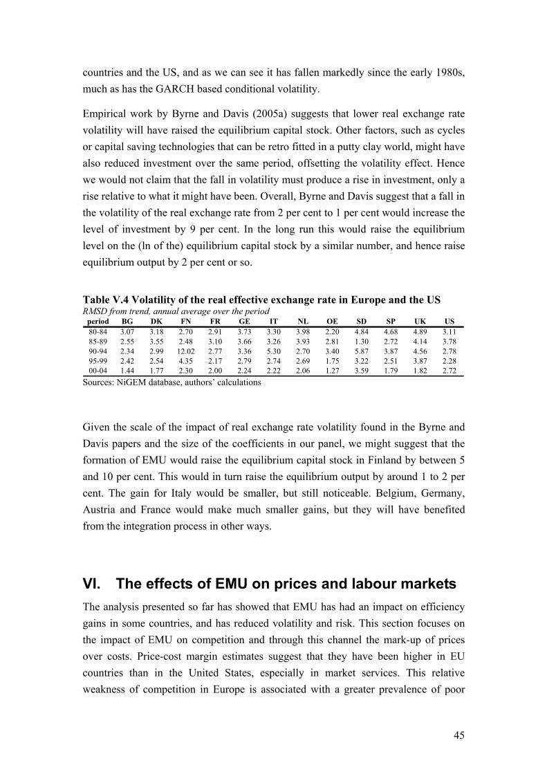
45
countries and the US, and as we can see it has fallen markedly since the early 1980s, much as has the GARCH based conditional volatility.
Empirical work by Byrne and Davis (2005a) suggests that lower real exchange rate volatility will have raised the equilibrium capital stock. Other factors, such as cycles or capital saving technologies that can be retro fitted in a putty clay world, might have also reduced investment over the same period, offsetting the volatility effect. Hence we would not claim that the fall in volatility must produce a rise in investment, only a rise relative to what it might have been. Overall, Byrne and Davis suggest that a fall in the volatility of the real exchange rate from 2 per cent to 1 per cent would increase the level of investment by 9 per cent. In the long run this would raise the equilibrium level on the (ln of the) equilibrium capital stock by a similar number, and hence raise equilibrium output by 2 per cent or so.
Table V.4 Volatility of the real effective exchange rate in Europe and the US RMSD from trend, annual average over the period
period BG DK FN FR GE IT NL OE SD SP UK US80-84 3.07 3.18 2.70 2.91 3.73 3.30 3.98 2.20 4.84 4.68 4.89 3.1185-89 2.55 3.55 2.48 3.10 3.66 3.26 3.93 2.81 1.30 2.72 4.14 3.7890-94 2.34 2.99 12.02 2.77 3.36 5.30 2.70 3.40 5.87 3.87 4.56 2.7895-99 2.42 2.54 4.35 2.17 2.79 2.74 2.69 1.75 3.22 2.51 3.87 2.2800-04 1.44 1.77 2.30 2.00 2.24 2.22 2.06 1.27 3.59 1.79 1.82 2.72
Sources: NiGEM database, authors’ calculations
Given the scale of the impact of real exchange rate volatility found in the Byrne and Davis papers and the size of the coefficients in our panel, we might suggest that the formation of EMU would raise the equilibrium capital stock in Finland by between 5 and 10 per cent. This would in turn raise the equilibrium output by around 1 to 2 per cent. The gain for Italy would be smaller, but still noticeable. Belgium, Germany, Austria and France would make much smaller gains, but they will have benefited from the integration process in other ways.
VI. The effects of EMU on prices and labour markets The analysis presented so far has showed that EMU has had an impact on efficiency gains in some countries, and has reduced volatility and risk. This section focuses on the impact of EMU on competition and through this channel the mark-up of prices over costs. Price-cost margin estimates suggest that they have been higher in EU countries than in the United States, especially in market services. This relative weakness of competition in Europe is associated with a greater prevalence of poor

46
management practices which translates into lower levels of total factor productivity (Bloom and van Reenen, 2006). Increased competition leads to lower mark-ups and more efficient production.
Theoretical work suggests that if price-cost margins in the Euro Area were reduced to American levels, real GDP would rise by 8.6 per cent and hours worked by 4.5 per cent, so that real GDP per hour worked would be about 4 per cent higher (Bayoumi, Laxton and Pesenti, 2004). Hence it is important to look at the determinants of the price-cost markup which allow us to determine if there has been an impact from EMU on the equilibrium level of employment. It is useful to have a simple description of the labour market and the determination of equilibrium unemployment. We develop the Layard, Nickell and Jackman (2006) framework where equilibrium unemployment follows on from the wage bargain and price setting. They assume that wages are set in bargains between employers and employees and depend in the long run on productivity and labour market institutions. The adjustment of wages to equilibrium depends on the level of excess unemployment, and on expectations of and inertia in response to price changes, which also depend on institutions.
It is unlikely that there is a direct role for EMU in the wage equation, but equilibrium employment depends on the bargaining based wage equation and on the price equation, and there should be a role for competition and liberalisation through their impact on prices. Analytically equilibrium unemployment is the solution to the long run aggregate price equation and the long run aggregate wage equation. The exact specification of the wage equation will depend on the wage formation process assumed, but in most cases can take the following general form:
W = Pe Z- φU (Q/L)β (10)
where U is the unemployment rate, φ reflects the search effectiveness or quality of the unemployed, Z incorporates other factors that are thought to affect wage setting such as the benefit replacement rate or skills mismatch, and β is a parameter which depends on the wage formation process assumed and the production technology. The long-run price equation can be based around a cost minimization problem. This leads to a long-run marginal cost equation22 that can be expressed as:
( ) ( ) techcLQbWaMC *ln*lnln +⎟⎠⎞
⎜⎝⎛++= (11)
where W is the wage, Q is output at basic prices and L is the labour input in hours. The marginal unit cost of production (MC) is an unobserved variable. Basic prices (P)
22 Holland (2007) develops this for the general CES case, and we use the marginal cost data from that study. The approach is consistent with out productivity analysis in section IV.

47
include a mark-up over marginal costs, reflecting product market competition and demand pressures. The mark-up should include a measure of the output gap or spare capacity, so that prices adjust to equate supply and demand. When demand is high and capacity constraints are tight, prices rise, while they fall when demand is weaker than supply. Competition depends on things such as product market regulation, globalisation and transparency. As the market place becomes more open, imported goods can be more easily substituted for domestically produced goods, putting downward pressure on the mark-up. Increased transparency may also support competition, and this may be related to factors such as the introduction of a single currency in the Euro Area. Prices may be written:
)ln()ln( MCmarkupP += (12)
An expression for equilibrium unemployment can be obtained by equating equations (10) and (12) and solving for U, and is a function of the markup as well as φ and Z.
Our key interest lies in the determinants of the mark-up, as this is the most likely route for EMU to affect equilibrium employment, and we will also test for roles of variables that capture capacity constraints, trade liberalisation, openness and transparency. Our model of the mark-up can be expressed as:
OPENWTONaftaEMUESMOGmarkup 654321 )ln( αααααα +++++= (13)
where OG is a measure of capacity constraints, SMP is an indicator of the European Single Market, EMU represents the introduction of the euro as currency, Nafta represents the North American Free Trade agreement, WTO is a global measure of trade liberalisation, and OPEN is a country-specific indicator of openness23. The measure of capacity constraints that we employ, OG, is NIESR’s estimate of the output gap, centred around 1. The estimated long-run parameter on this variable, α1, can be interpreted as the inverse of the price elasticity of demand, as prices adjust to bring demand in line with supply..
23 Our indicators of the establishment of the European Single Market, SMP, the introduction of the euro, EMU, and Nafta are compatible with those used in previous sections

48
Figure VI.1. Index of globalisation (WTO)
0.80
0.82
0.84
0.86
0.88
0.90
0.92
0.94
0.96
1976
q119
78q2
1980
q319
82q4
1985
q119
87q2
1989
q319
91q4
1994
q119
96q2
1998
q320
00q4
2003
q120
05q2
shar
e of
wor
ld tr
ade
cond
ucte
d by
WTO
/GA
TT
mem
bers
Figure VI.2. Openness indicator (OPEN)
0
0.2
0.4
0.6
0.8
1
1.2
1.4
FN FR GE IT NL SD UK US
tota
l tra
de re
lativ
e to
GD
P
1981 2004
Our key indicator of globalisation and global trade liberalisation (WTO), reflects the share of world trade conducted by members of WTO from 1995, and prior to 1995 the share of world trade conducted by the contracting parties of GATT. Figure VI.1 illustrates that it has clearly been on an upward trend over the full sample period, but there are some drops in the series. For example, the rise of China in global trade preceded its entry into the WTO, which explains much of the deterioration 1997-2000. Figure VI.2 illustrates the measure of openness (OPEN) which is calculated as total exports and imports of goods and services as a share of GDP, calculated in nominal terms. This has increased by 5-15 per cent in most countries over the sample period, with more significant rises in Germany, Sweden and the US.
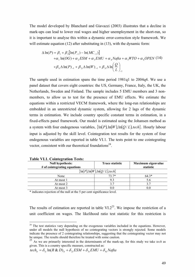
49
The model developed by Blanchard and Giavazzi (2003) illustrates that a decline in mark-ups can lead to lower real wages and higher unemployment in the short-run, so it is important to analyse this within a dynamic error-correction style framework. We will estimate equation (12) after substituting in (13), with the dynamic form:
[ ]
131211
654321
1121
ln)ln()ln(
)ln()ln()ln()ln(
−−−
−−
⎟⎠⎞
⎜⎝⎛Δ+Δ+Δ+
++++++−+=Δ
LQWP
OPENWTONaftaEMUESMOGMCPP
iii βββ
ααααααββ
(14)
The sample used in estimation spans the time period 1981q1 to 2004q4. We use a panel dataset that covers eight countries: the US, Germany, France, Italy, the UK, the Netherlands, Sweden and Finland. The sample includes 5 EMU members and 3 non-members, to allow us to test for the presence of EMU effects. We estimate the equations within a restricted VECM framework, where the long-run relationships are embedded in an unrestricted dynamic system, allowing for 2 lags of the dynamic terms in estimation. We include country specific constant terms in estimation, in a fixed-effects panel framework. Our model is estimated using the Johansen method as a system with four endogenous variables, ( ) ( ) ( ){ }techLQWP ,/ln,ln,ln . Hourly labour
input is adjusted by the skill level. Cointegration test results for the system of four endogenous variables are reported in table VI.1. The tests point to one cointegrating vector, consistent with our theoretical foundations24.
Table VI.1. Cointegration Tests:
Null hypothesis: # of cointegrating equations
Trace statistic Maximum eigenvalue statistic
( ) ( ) ( ){ }techLQWP ,/ln,ln,ln None 73.7* 64.3*
At most 1 9.3 5.6 At most 2 3.7 3.7 At most 3 0.0 0.0
* indicates rejection of the null at the 5 per cent significance level.
The results of estimation are reported in table VI.225. We impose the restriction of a unit coefficient on wages. The likelihood ratio test statistic for this restriction is
24 The test statistics vary depending on the exogenous variables included in the equations. However, under all models the null hypothesis of no cointegrating vectors is strongly rejected. Some models indicate the presence of 2 cointegrating relationships, suggesting that the cointegrating vector may not be unique. The results should therefore be treated with some caution. 25 As we are primarily interested in the determinants of the mark-up, for this study we take tech as given. This is a country specific measure, constructed as:
NaftaEMUESMDRtech iiiitiit 4321 )&ln( δδδδ +++=

50
reported in the table. We report results for three different models of the mark-up. Our first model restricts the determinants of the mark-up to the capacity indicator and the regional integrations measures, SMP, EMU and Nafta. The second model adds the global trade liberalisation measure, and the third equation adds the country-specific measure of openness.
Table VI.2. Estimated VECM’s for basic prices
Model 1 Model 2 Model 3 Cointegrating marginal cost equation
ln(P-1) 1 1 1 ln(W-1) -1 -1 -1
ln((Q/L)-1) 6.2 (10.1) 5.8 (10.7) 6.0 (10.4) tech-1 -5.9 (7.7) -5.9 (8.6) -6.1 (8.6)
Error Correction Δln(P) -0.010 (3.8) -0.011 (4.0) -0.011 (4.1)
Determinants of the mark-up ln(og) 0.11 (4.5) 0.12 (4.8) 0.12 (4.6) SMP
FN,FR,GE,IT, SD,UK -0.0096 (8.9) -0.0094 (7.3) -0.0098 (7.4)
EMU FN,FR,GE,IT,NL
-0.0003 (0.4) -0.0007 (0.9) -0.0014 (1.5)
Nafta (US) -0.0057 (3.3) -0.0057 (3.0) -0.0062 (3.2) WTO - -0.030 (3.2) -0.026 (2.7) OPEN - - 0.007 (1.5)
LR test for binding
restrictions (rank=1) χ2(1)=12.2
(p value= 0.00) χ2(1)=2.49
(p value= 0.11) χ2(1)= 3.01
(p value= 0.08) Adj. R-squared 0.46 0.47 0.47
AIC -30.00 -30.02 -30.01 Schwarz criterion -29.46 -29.46 -29.43
t-statistics in parentheses. Country-specific fixed effects were included in estimation, with 2 lags of the dynamic endogenous variables. Sample: 81q1-2004q4
The estimation framework adopted imposes a common long-run relationship and common speed of error correction across countries. We tested for differences across countries in the parameters on the determinants of the mark-up, but generally found that they are not significantly different from one another. The exception is the parameter on SMP for the Netherlands, which is insignificant and incorrectly signed. We therefore impose this parameter at zero for the Netherlands.
The parameter on the error-correction term is well determined, with a t-statistic of -3.8 to -4.1, supporting the test results that indicate a cointegrating relationship. The speed of adjustment suggests that about 4-4½ per cent of the deviation from equilibrium is corrected per annum. This suggests that it can take several years for the full effects of liberalisation to feed through into the price level.

51
• The parameter on the output gap, which brings aggregate demand and supply into line, suggests a price elasticity of demand of about -0.1, so that a 1 per cent rise in the price level reduces aggregate demand by about 0.1 per cent26..
• The parameter on the European Single Market indicator is significant, except in the case of the Netherlands, and indicates that as the single market progressed, competition increased in Finland, France, Germany, Italy, Sweden and the UK, and had a negative impact on the mark-up of prices over costs. The magnitude of the parameter suggests that overall impact of the integration process that took place between 1987 and 1992 should lower the price level of the European economies by about 20 per cent in the long-run. However, this impact feeds through very gradually, perhaps reducing annual inflation by an average of 0.7 percentage points per annum, holding everything else constant.
• The regional integration associated with NAFTA has had a significant impact on competition and the mark-up of prices over costs in the US, although the magnitude of the estimated impact is smaller than in the European Union.
• The inclusion of the global trade liberalisation measure, WTO, marginally improves the fit of the equation, but clearly improves the specification of the model, as the long-run restriction on wages is not rejected at the 5 or 10 per cent level. The estimated parameter on WTO is negative, indicating that increased globalisation has put downward pressure on the mark-up. There is little change to the other estimated parameters when this variable is added to the model. The point estimate of the parameter on WTO suggests that a 0.01 percentage point rise in our index of globalisation reduces the price level by about 0.03 per cent in the long-run. Over the sample period this index has been rising by roughly 0.1 percentage points a year, pointing to a cumulative long-run impact of -0.3 per cent on the price level.
The final model we consider includes our measure of openness (OPEN). The parameter on openness is not significantly different from zero, and the point estimate is the wrong sign. We, therefore, accept Model 2 as our preferred equation. While openness has not reduced price margins, it may have increased growth through its impacts on R&D and the state of technology.
The introduction of the euro itself, and the increased transparency associated with EMU, does not appear to have had a significant impact on price levels in the Euro Area economies, although the point estimate is correctly signed. Hence we cannot identify a clear impact from EMU on the equilibrium employment rate. Trade 26 To calculate the implied price elasticity of demand we first calculate the implied long-run parameter on ln(og), dividing the estimated parameter by the speed of adjustment. The implied price elasticity of demand is the reciprocal of this figure multiplied by -1.

52
liberalisation, both at the regional and global level, on the other hand, has significantly reduced price mark-ups in Europe and the US, and has raised the sustainable level of employment.
VII. Conclusions To date there has been little evidence on the impact of Monetary Union in Europe on output and growth. This is in part because the time period between the formation of EMU and the current date is short. It is also because there have been a number of other factors affecting growth that have to be taken into account before evaluating the impact of the Union. Most studies look either at a single driver of growth, or at one of the proximate determinants of growth, and look for EMU impacts on that proximate driver. Trade effects have been the most widely discussed, but it is not clear that even if EMU has increased trade between members that this will have a major impact on growth. We argue that only a study that takes into account other factors driving growth could uncover the potential effects on EMU on output, and we do that here.
Our analysis of the impact of EMU on output growth suggests that the introduction of the common currency has had a direct positive impact on growth in the core Euro Area countries: France, Germany, Italy, Belgium and the Netherlands. Our estimates indicate that EMU will eventually directly raise output level by around 2 per cent in these countries. This is smaller than the impact of the Single Market Programme in the late 1980s and early 1990s, and like those effects it will build up only slowly.
These findings are robust to the inclusion of other variables that have been driving growth such as R&D and FDI stocks and after adjusting the labour force for differences in skills levels across countries. After accounting for EMU, the European Single Market and the North American Free Trade Agreement, NAFTA, we found that openness, as measured by a share of total trade in output, had no significant direct role in explaining output or growth in our panel of countries. We were also able to show that the EMU effects were absent from countries such as the UK, the US, Denmark and Sweden who were not members. It is not clear that there were present in small economies such as Finland and Austria which may suggest that EMU has promoted agglomeration to the core of the Union.
The positive impact of EMU on long term growth is in contrast to the widely discussed relatively slow growth in the Euro Area. Much of this slower growth is in underlying productivity per person hour, and it reflects the differences in the rate of accumulation of skills across the countries we study. Around a quarter of a percentage

53
point of the difference in growth rates between the UK and the members of the Euro Area comes from the more rapid accumulation of skills in the UK, both in the run up to EMU and in the subsequent period. Skills growth was particularly slow in Germany and in Italy especially in the EMU period and this alone would account for half a percentage point difference in the growth rates between these countries and the UK.
Our panel analysis of the determinants of growth also point to the importance of the stock of R&D, and this has been growing more slowly in Italy than in any other Euro Area country except perhaps than the Netherlands. The lack of growth in skills and in knowledge together with the adverse effects of the recent liberalisation of world trade that have particularly affected Italian output are the main factors behind that countries slow growth. In addition our work suggests that the positive benefits of EMU will come through more slowly in Italy than in any other country we study except France.
Apart from estimating its direct effects on output, we investigated the impact of EMU on output through alternative channels, as suggested in the existing literature. Our results indicate that EMU may raise output by reducing output volatility, as EMU was found to have a significant impact on output volatility in most Euro Area economies including the small peripheral members. This suggests that the periphery still benefits from joining EMU through the reduction in output volatility.
Our analysis of volatility indicates that EMU has reduced the volatility of the real effective exchange rate for all members and especially for Finland where direct effects may not be present. In the long run, reduced uncertainty as regards the real effective exchange rate is thought to raise investment and capital stock relative to what it would have been in the absence of a monetary union in all member countries. It is difficult to extract this long run effect directly from such a short data sample, and we would argue that the impacts of EMU would be increased by around one percent of GDP in the larger countries and perhaps more in the smaller ones such as Finland. This would leave our range of estimated effects between one and a half and three percent of GDP per person hour.
As regards the impact of EMU on the amount of labour employed, Holland (2007) has not found that the transparency associated with the euro has had a significant impact on the mark-up and hence on the sustainable level of employment. At least as importantly, trade liberalisation, both on a global and European scale have reduced mark-ups, and that liberalisation has had a clear effect on the sustainable level of employment in the European countries. These results are repeated in this paper using a data set and asset of assumptions consistent with our core productivity analysis.

54
References Aghion, P., Bacchetta P.,. Ranciere R. and K. Rogoff (2006). Exchange Rate
Volatility and Productivity Growth: The Role of Financial Development, NBER, 52 pp.
Aghion, P. and Howitt, P. (1998). Endogenous growth theory, MIT Press.
Badinger H., (2007). Has the EU's single market programme fostered competition? Testing for a decrease in mark-up ratios in EU industries, Oxford Bulletin of Economics and Statistics 69 (4): 497-519 AUG 2007.
Baele, L., Ferrando A., Hordahl P., Krylova E. and C. Monnet. (2004). Measuring Financial Integration in the Euro Area. Occasional Paper, European Central Bank.
Bagella, M., Becchetti, L. and Hasan, I. (2004). The anticipated and concurring effects of EMU: exchange rate volatility, institutions and growth, Journal of International Money and Finance, Vol.23, Issue 7-8, pp. 1053-1080.
Baldwin, R. (2006). The euro’s trade effects, ECB Working Paper Series, No. 594.
Barrell, R., (2007a). Economic Growth in Europe, National Institute Economic Review January 2007 pp 65 -68.
Barrell, R., (2007b). The Future of Monetary Union in Europe, presented at the European Studies Institute, Birmingham University March 2007.
Barrell, R, Guillemineau, C., and Holland, D., (2007). Decomposing Growth in France, Germany and the UK using growth accounting and production function approaches, National Institute Economic Review January 2007 pp 99 -113.
Barrell, R. and O. Pomerantz (2004). Oil Prices and the World Economy, Focus on European Economic Integration: Oesterreichische Nationalbank. 1/2004.
Barrell, R., Liadze, I. and Pomerantz, O. - Import Growth and the Impact of Globalisation, Presented at Project Link CASS conference Beijing May 2007 National Institute Discussion Paper no 294.
Barrell, R., Holland, D., Liadze, I. and Pomerantz, O. Fiscal Spillovers and Trade Relations in Europe , presented at MMF Cambridge University conference at Trinity College February 2007 and at an HM Treasury Seminar April 2007 National Institute Discussion Paper no 289.
Barrell, R. and Pain, N. (1997). Foreign direct investment, technological change and economic growth within Europe, Economic Journal, Vol. 107, pp 1770-1786.
Barrell, R. and Pain, N. (1998). Real exchange rates, agglomerations and irreversibilities: Macroeconomic policy and FDI in EMU, Oxford Economic Review of Economic Policy, Vol. 14, pp. 152-167.
Barrell, R. and Pain, N. (1999). Domestic institutions, agglomerations and foreign direct investment in Europe, European Economic Review, Vol. 43, pp. 925-934.
Barrell, R. and Pomerantz, O. (2004). Oil prices and the world economy, National Institute Discussion Paper, No. 242, pp 1-28.

55
Barrell, R. S. Gottschalk and S. Hall (2007). Foreign direct investment and exchange rate uncertainty in imperfectly competitive industries, in Korres (Ed.), Regionalisation, Growth and Economic Integration, Springer-Verlag, 2007.
Bayoumi,T., Douglas, L. and Pesenti, P. (2004). Benefits and spillovers of greater competition in Europe: a macroeconomic assessment, International Finance Discussion Papers, No 803, Board of Governors of the Federal Reserve System (U.S.)
Bertola, G. and T. Boeri (2002). EMU Labour Markets Two Years On: Microeconomic tensions and institutional evolution, in M.Buti and A.Sapir (eds.), EMU and Economic Policy in Europe: The Challenge of the Early Years, Edward Elgar, Aldershot.
Blanchard, O. and Giavazzi, F. (2003). Macroeconomic effects of regulation and deregulation in goods and labor markets, Quarterly Journal of Economics, Vol. 118, Issue 3, pp. 879-907.
Blanchard, O. and Simon, J. (2001). The long and large decline in US output volatility, Brookings Papers on Economic Activity, No.1, pp 135-174.
Bloom, N. and van Reenen, J. (2006). Measuring and Explaining Management Practices Across Firms and Countries, CEP Discussion Paper, No 716.
Boeri, T. (2005). Reforming Labor and Product Markets: Some Lessons from Two Decades of Experiments in Europe, IMF Working Papers, 05/97.
Brealey, R.A. and Myers, S.C. (2005). Investment and uncertainty in the G7, Review of World Economics, Vol. 41, No. 1, pp 1-32.
Bun, M. and F. Klaasen (2003). Has the euro increased trade?, Tinbergen Institute Discussion Paper, No 02-108/2.
Byrne, J.P. and Davis, E.P. (2005 b). Investment and uncertainty in the G7, Review of World Economics, Vol. 41, No. 1, pp 1-32.
Byrne, J.P. and Davis, E.P. (2005a). The impact of short- and long-run exchange rate uncertainty on investment: A panel study of industrial countries, Oxford Bulletin of Economics and Statistics, Vol. 67, No. 3, pp 307-329.
Cappiello, L., Engle. R. and K. Sheppard, (2006). Asymmetric Dynamics in the Correlations of Global Equity and Bond Returns. Journal of Financial Econometrics 4, pp. 537-572.
Carruth, A., Dickerson, A. and Henley, A. (2000). What do we know about investment under uncertainty?, Journal of Economic Surveys, Vol. 14, No. 2, pp 119-153.
Chakrabarti, R. and B. Scholnick (2002). Exchange rate regimes and foreign direct investment flows, Weltwirtschaftliches Archiv, Vol. 138, pp.1-21.
Coe, D. and Helpman, E. (1995). International R-and-D spillovers, European Economic Review, Vol. 39, No. 5, pp 859-887.
Crafts N. (2007). Recent European economic growth: why can’t it be like the Golden Age?, National Institute Economic Review, No. 199, pp. 69-81.
Cushman, D.O. (1985). Real exchange rate risk, expectations and the level of direct investment, Review of Economics and Statistics, Vol. 67, pp.297-308.
56
Cushman, D.O. (1988). Exchange rate uncertainty and foreign direct investment in the United States, Weltwirtschaftliches Archiv, Vol. 124, pp.322-336.
Dunning J. (1997). The European internal market programme and inbound foreign direct investment, Journal of Common Market Studies, Vol. 35, Issue: 1, pp. 1-30.
Darby, J., Hughes Hallett, A., Ireland, J. and Piscatelli, L. (1999). The impact of exchange rate uncertainty on the level of investment, Economic Journal, Vol. 10 (454), pp 55-67.
Davidson J. (1998). Structural relations, cointegration and identification: some simple results and their application, Journal of Econometrics, 87, pp. 87-113.
Delbecque, V. and A. Larèche-Révil (2007). Do EU member states compete on social systems?, presented at the June 2007 Euroframe Conference. http://www.euroframe.org/fileadmin/user_upload/euroframe/docs/2007/session3/EUROF07_Patureau.pdf.
Durbin, J. (1954). Errors in variables, Review of International Statistics Institute, Vol. 22, pp 23-32.
Duval, R. and Elmeskov, J. (2006). The effects of EMU on structural reform in labour and product markets, ECB Working Paper Series, No. 596.
European Commission (2004). EMU after five years, Economic and Financial Affairs Publications, Special Report 1/2004, pp 1-260.
European Parliament Fact Sheets - 3.1.0. Principles and general completion of the internal market.
Giannone, D. and Reichlin, L. (2006). Does information help recovering structural shocks from past observations?, Journal of the European Economic Association, MIT Press, vol. 4(2-3), pages 455-465, 04-05.
Goldberg, L.S. and C.D. Kolstad (1995). Foreign direct investment, exchange rate variability and demand uncertainty, International Economic Review, Vol. 36, pp.855-873.
Görg, H. and K. Wakelin (2002). The impact of exchange rate volatility on US investment, Manchester School, Vol. 70, n o 3, pp. 380-397.
Griffith, R., Redding, S. and Van Reenen, J. (2004). Mapping the two faces of R&D: Productivity growth in a panel of OECD industries, Review of Economics and Statistics, Vol. 86, No. 54, pp 883-895.
Holland, D. (2007). An estimation of the factors driving the mark-up of prices over costs, NIESR, mimeo.
Lane, P. (2006). The real effects of European monetary union, Journal of Economic Perspectives, Vol. 20, No. 4, pp 47-66.
Layard, R., Nickell, S. and Jackman, R. (2006). Unemployment, Oxford University Press.
Lederman, D., Serven L (2007). Tracking NAFTA's shadow 10 years on: Introduction to the symposium World Bank Economic Review 19 (3): 335-344 2005.

57
McMorrow, K. and Röger, W. (2007). An analysis of EU growth trends, with a particular focus on Germany, France, Italy and the UK”, National Institute Economic Review, No. 199, January 2007.
Micco, A., E. Stein and G. Ordonez (2003). The currency union effect on trade: Early evidence from EMU, Economic Policy, Issue 18, pp. 315-356.
Nickell, S. (2006). Comments on Duval and Elmeskov (2006). The effects of EMU on structural reform in labour and product markets, ECB Working Paper Series, No. 596.
Pagan, A. (1984). Econometric Issues in the Analysis of Regressions with Generated Regressors, International Economic Review, Department of Economics, University of Pennsylvania and Osaka University Institute of Social and Economic Research Association, vol. 25(1), pp. 221-47.
Pain, N. and G. Young (2003). The macroeconomic impact of UK withdrawal from the EU, Economic Modelling.
Pesaran, H. and Smith, R.P. (1995). Estimating long-run relationships from dynamic heterogeneous panels, Journal of Econometrics, Vol. 68, pp 79-113.
Petroulas, P. (2007). The effect of the euro on foreign direct investment, European Economic Review, Vol. 51, No. 6, pp 1468-1491.
Proudman, J. and Redding, S. (1998). Openness and growth, Bank of England.
Ricci, L. (1998). Uncertainty, flexible exchange rates and agglomeration, IMF Working Paper, no 98/9, IMF.
Rose, A. (2000). One money, one market: Estimating the effect of common currencies on trade, Economic Policy, Issue 30, pp.9-45.
Sekkat, K. and O. Galgau, (2001). The impact of the Single Market on foreign direct investment in the European Union, mimeo, DULBEA, Université Libre de Bruxelles.
Wyplosz, C. (2006). European Monetary Union: the dark sides of a major success, Economic Policy, Vol. 21, No. 46, pp 207-261.
Zhang, L.H. (2001). Did European integration attract more foreign direct investment?, Mimeo, John Hopkins University.

58
Appendix. Data description and sources E – Total employment (thousands). Data source Datastream. FDI – Stock of foreign direct investment in the country (in constant prices and national currencies). Source UNCTAD. http://unstats.un.org. H – Hours worked per employee per quarter. Data source OECD, http://www.sourceoecd.org. INFL – 100 plus inflation rate. Data source Datastream and NiGEM database. MC –The marginal unit cost of production. OG – Output gap. Data source NiGEM database. P – Basic prices, include a mark-up over marginal costs. Data source NiGEM database. Q – GDP in basic prices. Data source NiGEM database. R&D – Stock of Research and Development. We benchmark the stock in 1974, before the beginning of our data period, as the flow divided by the average growth rate and the depreciation rate, and we cumulate flows onto this stock with a depreciation rate of 5 per cent per annum. The data souse is OECD Science and Technology database. Refex – Real exchange rate. Data source NiGEM database. R3M – 100 plus 3-month nominal interest rate. Data source NiGEM database. S – Average skills of the workforce is a compound skill indicator which uses indicators of relative wages for each of three (high, medium and low) skill groups to weight together the numbers employed in each skill group to give a weighted average skill indicator. We assume that the wage of unskilled workers is1.0 in a base year 1992. Data comes from EUKLEMS database, http://www.euklems.net/. USER – User cost of capital. Data source NiGEM database. W – wages. Data source NiGEM database. Y – GDP in constant market prices. Data source Datastream. Voly – Volatility of output. Constructed as a root mean square deviation of GDP around a 17 quarter centred moving average. Volrefex – Volatility of real exchange rate. Constructed as a root mean square deviation of real exchange rate around a 13 quarter centred moving average.
59
ESM – Describes the establishment of the European Single Market. This variable is equal to zero prior to 1987Q2 which gradually increases to one in 1992Q4, the formal completion of the Single Market Programme. EMU – Is meant to capture the impact of the European Monetary Union. It is a dummy variable which equals to 1 from 1999Q1, in line with the official introduction of single currency in Europe and is zero prior to 1999. EU – Is meant to take an account of the impact on country upon joining the European Union (EU). It is a variable moddeled to be zero before the country in question joining the EU and one thereafter. NAFTA – The North American Free Trade Agreement variable is created to account for the impact of gradual elimination of tariffs on the goods shipped between US, Canada and Mexico. As NAFTA agreement represented an expansion of the earlier Canada-U.S. Free Trade Agreement of 1988, the NAFTA variable is equal to zero before 1989Q1 and is increased to one by 1998Q1. OPEN – Is a measure of the openness of the economy and defined as exports and imports of goods and services as a share of GDP. Data source NiGEM database. WTO – Is a measure of globalisation and global trade liberalisation. Reflects the share of world trade conducted by members of WTO from 1995, and prior to 1995 the share of world trade conducted by the contracting parties of GATT. Data source WTO annual report.