The Impact of Institutions on Economic Growth in Economies with

Poverty Traps: An Experimental Approach

C. Monica Capra, Colin Camerer, Lauren Munyan, Veronica Sovero, Tomomi Tanaka, Lisa

Wang, and Charles Noussair1

1. Introduction Income levels and rates of economic growth differ widely among different countries. While

some of these differences may be attributed to variation in resource endowments and geographic

location (Sacks and Warner, 1995), it is also recognized that institutions, such as the system of

government, freedom of the press, and an independent central bank, play an important role in

explaining international economic disparities (Baumol, 1986; Barro and Sala-i-Martin, 1995; Barro,

1997). However, identifying the precise impact of a particular institution is typically very difficult.

Institutions as observed in the world arise endogenously, rather than randomly, so that there is an

inherent sample bias when attempting to attribute economic performance to institutional differences2.

Institutions also tend to occur in clusters making it difficult to isolate the effect of a particular

institution on economic growth. For example, the incidence of democratic electoral systems and press

freedom are highly correlated. Furthermore, there are country-specific cultural and social factors that

are difficult to quantify, which interact with institutions and may affect economic performance

(Acemoglu et al, 2001; Knack and Keefer, 1999). Episodes of institutional change, which in principle

provide opportunities to compare economic performance before and after the change, are also

problematic to study, because the change itself is endogenous, presumably depending at least in part

on the performance of the institutions or policies in effect before the change.

The essential difficulty that impedes the systematic study of the marginal effects of individual

institutions in isolation on economic growth is that the researcher is unable to control the environment

in which the institution is applied. Rather, the researcher is restricted to the conditions that exist in the

countries he can observe. In this paper, we take a new approach to the study of the effect of

institutions on income levels in macroeconomies. We use laboratory experimentation to study the

1 Capra and Noussair: Department of Economics. Emory University, 1602 Fishburne Dr, Atlanta, GA, 30322-2240, USA. Camerer, Munyan, Sovero, Tanaka, and Wang: Department of Economics, California Institute of Technology, 91125. 2 See Temple (1999), Islam (2003) or Durlauf and Quah (2003) for a discussion of empirical methodology and results with regard to international comparisons of rates of economic growth.

1

effect of institutions on economic growth. We construct experimental macroeconomies in which

simple (and highly stylized) versions of basic institutional structures are applied. Their performance,

in terms of output, welfare, and consumption, is compared with each other and with theoretical

benchmarks.

This study is appropriately viewed as a first foray into the topic. To begin such a program of

research, we have chosen to study an environment that is relatively well understood theoretically, and

which contains only a few of the basic characteristics of field macroeconomies. No attempt is made at

this stage to simulate actual countries as observed in the field, or to capture cultural factors,

international relations, geopolitics, and the complexity resulting from the enormous number of

heterogeneous goods or types of agent that exists in the field. This initial focus on a very simple

environment has several advantages. The first is that the calculation of theoretical benchmarks such as

competitive equilibria and social optima is facilitated. Moreover, we believe that studying economies

with the structure of a classical model at this stage of the research program is also the best way to

facilitate discussion between economists concerning how the determinants of economic growth might

be studied in a controlled, systematic manner.

Our experimental environment consists of a dynamic macroeconomy with two stationary

Pareto-ranked competitive equilibria.3 The environment is an extension of the optimal growth model

of Ramsey (1928), Cass (1965), and Koopmans (1965), and thus is well understood in terms of

theoretical properties.4 The environment in our experiment is also the same as that studied in the

laboratory by Lei and Noussair (2003), and thus the behavior of the economy is well documented in a

baseline environment with a minimal institutional structure. However, in contrast to the

Ramsey/Cass/Koopmans model, there is a threshold level of capital known to all subjects that must be

accumulated to allow convergence to the better equilibrium. The better equilibrium has the property

that each individual enjoys higher consumption and higher utility than in the inferior equilibrium,

3 See Plott and George (1990) for a experimental study of one-period markets in which there are two competitive equilibria. 4 According to the Ramsey/Cass/Koopmans model (Ramsey, 1928; Cass, 1965; Koopmans, 1965), countries that have access to the same production technology would converge toward a common income level even if their initial endowment of capital differed; thus, relatively poor countries would exhibit higher growth rates than richer ones. However, field studies have generally failed to support the hypothesis of convergence towards a common income level (see Temple, 1999; Durlauf and Quah 2001; and Islam, 2003 for surveys). Indeed, the data are more consistent with the alternative hypothesis of club convergence (Baumol, 1986), which postulates that a small number of steady states exists, and that each country has a tendency to converge to one of them. Such a framework can explain the observed pattern over time of both an increase in income differences between the OECD countries and the developing world and a decrease in the differences within each of the two groups.

2

which can be viewed as a technological poverty trap.5 The parametric structure of the economy and

the initial endowments are chosen so that the poverty trap would be likely to be reached in a

decentralized economy (Lei and Noussair, 2003), in the absence of additional institutions. Institutions

are added to the economy and tasked with allowing the economy to avoid or to exit the poverty trap,

in an environment in which considerable potential for improvement of outcomes exists. The

institutions chosen are highly stylized versions of two institutions that are generally believed to

enhance economic growth in the field and are thought to facilitate the solution of equilibrium

selection problems. The different institutions are introduced into our decentralized economies holding

all other aspects of the environment constant.

The first institution we consider is a highly stylized version of freedom of expression. In the

experiment, this takes the form of allowing any agents in the economy to make unrestricted public

announcements in each period. The second institution is an, again highly stylized, version of a

democratic voting process. A subset of agents is permitted to submit policy proposals, between which

the citizens populating the economy vote, with majority rule determining which of the proposals is

implemented. The focus of our analysis is on whether the freedom to communicate leads to higher

income, whether the voting system we study leads to higher income, and whether there is an

interaction effect between the two instruments. We also conduct an exploratory analysis of the data at

both the aggregate and at the individual levels in an effort to understand the origins of the differences

in performance between institutions.

Of course, our results are specific to our particular economy. We are not attempting to

simulate any particular economies, or to reproduce the precise institutional structures that are found in

the field. The objective is to begin to systematically study the empirical properties of institutions in

dynamic macroeconomies. We begin with very simple institutions in very simple economies, and the

terms “free expression” and “democratic voting” as used in this paper describe the institutions in

effect in the experiment, and should not be interpreted as analogous to institutions that may be

assigned these labels in the field. To yield practical insights for institutional design in field

5 Theoretically, the absence of convergence can be explained by models with multiple competitive equilibria. Originally attributed to Rosenstein-Rodan (1943), this idea has led a rich variety of growth models. For instance, Azariadis and Drazen (1990) construct an overlapping generations model with two stable Pareto-ranked equilibria. In the inferior equilibrium, no agent trades with members of other generations. Murphy et al. (1989) build a model with synergies among industries, where each industry is profitable only if other industries operate; there are Pareto-dominant equilibria where all of the industries operate and dominated equilibria where none operate. Galor and Zeira (1993) and Banerjee et al. (2001) show that inequality and the resulting differential access to credit among members of the population can keep an economy in a Pareto dominated equilibrium. See Azariadis (1993) and Cooper (2002) for a detailed treatment of the principal analytical issues in growth models with multiple equilibria.

3

environments requires robustness checks under different, more complex economic environments and

under related institutional structures. It also requires plausible general conjectures about the properties

of different institutions and how these properties are generalized or modified as the structure of the

economy or the rules of the institution change. The research reported here is a step in developing a

new methodology to study existing, and to design new, macroeconomic institutions. The economy,

the theoretical predictions, and the procedures of the experiment are described in section two. In

section three the results are reported, and in section four, we provide a summary and some thoughts

about future research.

2. The experimental environment, competitive equilibria, and procedures 2.1. The environment

The environment is similar in parametric structure to that of the economies of Lei and

Noussair (2003), although the institutions that guide economic activity differ from theirs. In the

experiment, activity occurs over a discrete series of periods, and under a random ending rule that is

equivalent in principle to an infinite horizon. At an aggregate level, the economy may be thought of

as being populated by an infinitely-lived representative consumer with a lifetime utility given by:

∑ , (1) )()1(0

∞

=

−+t

tt CUρ

ρ is the discount rate, Ct is the quantity of consumption at time t, and U(Ct) is the representative

consumer’s utility of consumption. Alternatively, the expression in equation (1) may be thought of as

the total value that an infinitely-lived group of agents receives from consumption. The economy faces

the following resource constraint:

C tttt KKFAK )1()(1 δ−+∗≤+ + , (2)

with

≥<

=KKAKKAA ˆ if ,

ˆ if ,. (3)

δ is the depreciation rate, Kt is the economy’s aggregate capital stock at the beginning of period t, and

A is an efficiency parameter on the production technology. The value of A depends on the current

level of capital stock in the economy. There exists a threshold level of capital stock, K̂ , above which

A has a value, A , and below which it has the value of A , with AA < . The threshold can be

4

interpreted as a positive externality in production, generated by a sufficiently large aggregate quantity

of capital stock in the economy.6

In our experiments, the economy-wide production technology is approximated by

for and 16 for . The aggregate utility of consumption at

time t is approximated by U . The utility function is expressed in terms of an

experimental currency, called “Yen,” which is converted to US dollars at the end of the experiment at

a predetermined exchange rate. The parameters

5.0*88.7 tK 31<tK 5.0*771. tK

2400) tt C −=

31≥tK

2)t(( CC

δ , ρ , and K0 are always equal to 1, 0.25, and 25

respectively.

In the experiment, the aggregate production capability and the value of consumption of units

are divided among five heterogeneous agents populating the economy. Each subject is given an

individual production schedule that outlines his or her ability to transform capital into

output . Each individual’s production schedule consists of two parts, corresponding to the

individual’s share of the aggregate production function for

itk

)(* it

i kfA

5.0*88.7 tK 31<tK

itc20

(where ), and to the case where 16 for respectively. The marginal

utility of consumption of agent i was thus a discrete approximation of v .

tiit Kk =∑ 5.0*771. tK 31

it

i c 396)(' =

≥tK

i4 −+

The individual and aggregate production functions are illustrated in figure 1. The first five

charts in the figure indicate the production technology available to each of the five individuals. If

aggregate capital stock is equal to 30 or less, the functions labeled “Below Threshold” are in force,

and if aggregate capital stock is greater than or equal to 31, the functions labeled “Above Threshold”

apply. The sixth chart is the aggregate production function, which would exist if all five producers

were merged into a single individual. The demand for consumption is illustrated in a similar manner

in figure 2. The five individual demand curves for consumption, which are equal to the five

individuals’ marginal utilities of consumption, are shown in the first five charts, and the sixth displays

aggregate demand.7 Each agent receives an initial endowment of ki0 = 5 for all i. See Lei and Noussair

(2003) for a more detailed description of the parametric structure.

6 See Azariadis (1993) and Azariadis and Drazen (1990) for discussion of growth models with a threshold externality in production. 7 As will be apparent from the discussion later in this section, the utility functions of each individual are quasilinear (concave in consumption, linear in money, and separable in the two arguments), and thus the corresponding indirect utilities have the Gorman form. Therefore, modeling the economy as a social planner maximizing the aggregate utility function U generates behavior that is consistent with maximizing any social welfare function that is monotonic and concave in each individual agent’s indirect utility.

)( tC

5

[Figures 1 and 2 About Here]

2.2. Competitive equilibria

The economy is structured in such a way so that there exist two stationary stable rational

expectations competitive equilibria. These serve as our primary benchmarks. One of these is optimal,

in the sense that it is equivalent to the outcome to which the economy would converge were it under

the direction of a benevolent social planner. Such as planner would choose C1… C∞ to maximize (1),

subject to (2), (3), and the constraints that Ct ≥ 0, Kt ≥ 0 and tt KK )1(1 δ−≥+

*

(gross investment in

every period must be non-negative). Lei and Noussair (2003) show that for the parameters of the

experiment, in which capital and consumption can only take on integer quantities, there are two stable

stationary competitive equilibria. These occur at ( )70 ,45()* , =HH CK

)70

and . is optimal in that from any initial level of capital stock K)16 ,9()* ,*( =LL CK )* ,*( HH CK 0

(including K0 = 9), the optimal sequence of consumption and investment decisions of a hypothetical

benevolent social planner converges to ( ,45()* ,* =HH CK

)70 ,45

. Thus, there is an optimal steady

state at . ()* ,*( =SPOSPO CK

The price of capital that supports the Pareto-optimal equilibrium is , and

is the price that supports the Pareto-inferior equilibrium. At the Pareto-optimal

competitive equilibrium, each agent consumes 14 units per period for an economy-wide total of 70

units of consumption, and the capital stock is distributed among the agents in the following manner:

118* =HP

334* =LP

121 =k , 9=2k , 63 =k , 84 =k , and 105 =k , where ik is the equilibrium capital holding of

agent i, yielding a total ∑ =5

145ik . At the Pareto inferior equilibrium agents 1 to 4 each consume 3

units and agent 5 consumes 4 units per period for a total consumption of 16. The allocation of capital

stock in this equilibrium is 11 =k , 22 =k , 13 =k , 24 =k , and 35 =k , yielding a total equilibrium

capital stock of 9 units.

2.3. Procedures

2.3.1. General procedures

The experiment consisted of a total of 21 sessions. There were four different treatments in the

experiment, and the four treatments differed from each other only in the institutional structures

6

guiding activity in the economy. The four treatments, described in detail in the next subsection are

called the baseline, communication, voting, and hybrid treatments. Each treatment will be described

in more detail in the next subsection. Participants were undergraduate students at Emory University,

located in Atlanta, Georgia, USA, and the California Institute of Technology, in Pasadena, California,

USA, and the sessions were conducted in dedicated experimental laboratories at the two universities.

Subjects were paid an initial fee that ranged from $5 to $10 for their participation, depending on the

session and their role in the game. Their additional earnings from their activity in the economies

described below ranged from $16 to $70. In all of the sessions, no subject had participated in a similar

experiment previously, although some of the subjects had previously participated in other, unrelated

experimental studies. The next three subsections briefly describe the experiment, and the instructions

in the appendix contain a more detailed explanation of the decision environment. Table 1 contains a

list of the sessions, the location they were conducted, and the average earnings of session participants.

2.3.2. Timing within a session

Five subjects participated in each session, and were grouped together in the same economy.

At the beginning of each session, the experimenter distributed and read aloud the instructions for the

experiment. The instructions for the hybrid treatment are given here as appendix A.8 The activity in

each session consisted of several horizons of random length and each horizon consisted of a series of

periods. The period of time defined by a horizon in the experiment corresponds to an infinite horizon

in the theoretical model of section 2.1. In the experiment, a random ending rule, in which the horizon

ended with a probability that was constant in each period, was used to induce a decision situation

equivalent to an infinite time horizon with discounting.9 Under the assumption that subjects in the

experiment are risk neutral in their final monetary payment, a constant probability of 20% of the

horizon ending in each period is equivalent to an infinite horizon in which 25.0=ρ . The

experimenter implemented the ending rule by rolling a die to determine whether or not the horizon

would terminate at the end of the current period. The number and length of each horizon in each

session is indicated in table 1.10

Each session was scheduled for a three-hour time interval for which subjects were recruited.

If the current horizon ended with more than 30 minutes remaining in the three-hour interval, a new

8 The instructions for the three other treatments are subsets of those of the hybrid treatment. 9 Other authors have used a similar rule to create the incentives of infinite horizon models in the laboratory. See for example Camerer and Weigelt (1993) or Noussair and Matheny (2000). 10 After the instructions were read, subjects participated in a three period practice horizon which did not count toward their earnings.

7

horizon was started with the same initial endowments, 5 units of capital and 10,000 per person, as in

the first horizon of a session. Thus a horizon, which corresponds to the life of the economy in the

theoretical model, is a distinct notion of time from an experimental session. Each session was

composed of several horizons and the number of horizons in our sessions ranged from 2 to 8. The

initial endowments for each horizon were independent of any activity in prior horizons. Restarting

with the same initial values after an exogenous random ending has no distortionary effect on optimal

decisions.

The instructions indicated that if a horizon did not terminate by the end of the third hour of a

session, it would be continued on another evening. Subjects would be free to return for that session

and continue in their same roles at the point at which they left off. If a subject was unwilling or

unable to return, a substitute would be recruited to replace him. The earnings the substitute made

would be awarded to the original subject as well as to the substitute himself. This technique, first

applied in Lei and Noussair (2002), preserves the incentive for subjects to make the as decisions that

they would if they were to participate until the end of the horizon, even when they would not actually

be participating when the horizon was continued in the future session. In no session of our experiment

was it actually necessary to continue on another day, as the three-hour time limit was not binding in

any session.

[Table 1 and Figure 3a-3d: About Here]

2.3.4. Timing within a period

The sequence of activities within each period for the four treatments is shown in figures 3a – 3d. The

tables also illustrate the differences between the treatments. In the baseline treatment, whose timing is

illustrated in figure 3a, each period consisted of two decision stages. In stage 1, subjects participated

in a market for capital. In stage 2, subjects chose how much of their capital to consume. More

specifically, the timing of events within a period were as follows: at the beginning of period t,

production occurred automatically as the computer program mapped kti, the capital stock that each

individual held, into output (cti + kt+1

i), according to the individual’s production function fi (kti). A

market for output then opened. The trading rules in effect in the market are described in subsection

2.3.5. After the market closed and transactions were realized, agents chose the portion of their output

to allocate to consumption cti. Before making their decisions, agents could use a simulator which

allowed them to study, by submitting hypothetical consumption and investment scenarios, how their

choice of cti affected their utility of consumption ui(ct

i), their remaining capital stock kt+1i, and how

much output they would have at the beginning of the next period f(kt+1i). The remaining output of

8

each individual, after her choice of consumption, became her kt+1i. At the beginning of period t+1,

production occurred as kt+1i was mapped into output (ct+1

i + kt+2i), according to the function f(kt+1

i), for

all i.

The sequence of events in a period under the communication treatment was identical to the

baseline treatment, except that before the market opened, subjects were allowed to communicate with

each other. Each agent’s screen displayed a chat-room, which he could use to send and receive

messages in real time. Communication was unrestricted in content and all agents could observe all

messages. Figure 3b illustrates the sequence of events in the communication treatment.

In the voting treatment, shown in figure 3c, the timing of events was identical to the baseline

treatment except that in stage 2, subjects’ consumption and investment decision were determined

differently from the baseline and the communication treatments. Two agents were randomly chosen

in each period to submit proposals on how much each agent in the economy would consume. A

proposal consisted of a five-element vector of consumption levels, one element corresponding to each

agent. Before submitting proposals, proposers received information indicating the current stock of

capital held by each agent. Proposers could use a simulator to see how hypothetical proposals affected

each individual’s consumption level, capital stock holdings at the end of the current period, and

available output at the beginning of the next period. The two proposals were submitted publicly and

appeared on each agent’s computer screen. All agents were then required to vote in favor of exactly

one of the two proposals. Majority rule determined the winning proposal. The proposal that gained at

least three of the five total votes was enacted. Each agent consumed the quantity of output specified

under the winning proposal, and began the next period with the amount of capital allotted to her under

the winning proposal.

Under the hybrid treatment, an opportunity for agents to exchange messages was available, as

in the communication treatment. Thus, the first stage of the hybrid treatment was identical to first

stage of the communication treatment. The second stage was identical to that of the voting treatment.

The sequence of events in a period of the hybrid treatment is shown in figure 3d.

2.3.5. The Market

In our economies, each agent received an endowment of cash, which he could use for

purchases and sales of output. The cash was not a fiat money, but rather was convertible to earnings

for the subject outside the experiment, at a conversion rate that was known to the individual in

advance, and thus the cash had intrinsic value. Since agents were not symmetric (i.e., their utility and

production functions differred from each other’s), gains from trade existed from the exchange of

9

output. During each period of each treatment, there was an interval of time in which a computerized

call market for capital was in operation.

The market operated in the following manner. In each period, all agents were required to

submit demand schedules that specified limit prices for each unit of capital that they wished to

purchase, and an aggregate demand schedule was constructed from the individual schedules. The

aggregate supply schedule of output was constant, corresponding to a vertical supply curve, at the

total amount of output in the economy for the current period Kt. The market-clearing price was

determined by the intersection of aggregate demand and supply and equaled the lowest accepted bid,

which was equal to the Ktth highest bid among all players. Agents who submitted limit prices greater

than or equal to the market-clearing price received the units of capital. Any tie for the Ktth highest bid

was broken by allocating the last units to the tied marginal bidders randomly in a way such that all K

units were allocated. When an individual had a net change in capital holding after the market process,

the agent either (a) paid a per-unit price equal to the market-clearing price for each unit he purchased,

or (b) received a per-unit price equal to the market-clearing price for each unit he sold.

In other words, the market reallocated output in the following manner. In period t each agent i

submitted a demand curve dit(p), where p was the price for output. An algorithm then calculated

Σidit(p), and solved for the price p* at which Σidi

t(p*) = Σifi(kti). Agent i’s final allocation of output

was equal to dit(p*). The net change in his holding of output was equal to di

t(p*) – fi(kti). Each agent i

received a cash transfer of p**[fi(kti) - di

t(p*)].

2.3.6. Initial Endowments and Agent Incentives

Each of the five agents received an initial endowment of five units of capital, so that

aggregate initial capital, , equaled 25. The initial endowments were chosen so that the poverty trap

would be likely to be reached in a decentralized market economy, in the absence of any additional

institution to aid economic performance. This conjecture, that the baseline treatment would converge

to the poverty trap, is based on the results of Lei and Noussair (2003). Each agent also received

10,000 units of experimental currency with which to make transactions. This cash endowment was

sufficient to ensure that cash constraints were unlikely to be binding at any point in time.

0K

Each agent’s earnings resulted from consumption and well as sales of output in the market. In

each period t, a player i’s earnings, in terms of experimental currency, were given by ui(cit) + mi1

t –

mi0t, where ui(ci

t) denotes individual i’s earnings from consumption, and mi1t and mi0

t respectively

denote i’s cash holdings at the beginning and the end of period t. Over each horizon, individual i’s

earnings were given by Σt[ui(cit) + mi1

t – mi0t], so that each individual had an incentive to hold some

10

output in the form of investment to allow consumption or sales in future periods. A player also had an

incentive to sell output if the price was high, in order to increase his end of period cash holdings, as

well as an incentive to purchase output at low prices either to consume, to produce more output in

future periods, or to resell at a higher price. Over an experimental session, a participant’s dollar

earnings were τi+ γi(ΣkΣt[ui(cit) + mi1

t – mi0t]). k indexes the horizon within a session, γi is agent i’s

conversion rate from experimental currency to US dollars, and τi is agent i’s fixed supplementary

payment for his participation in the experiment.11

2.4 Design and Hypotheses

The four treatments constitute a two-level two-factor experimental design, where the factors

are the institutions of communication and of voting, and the levels are the presence and the absence of

the institution. Before conducting the experiment, we advance several hypotheses to test in the data.

The first hypothesis is that the economies in the baseline treatment converge to the poverty trap, the

Pareto-dominated equilibrium. The basis for this hypothesis is the previous work of Lei and Noussair

(2003) who study a decentralized economy with the same parametric structure that closely resembles

the baseline treatment, and find a strong tendency for the economy to converge to the poverty trap.

The only difference between the economies that Lei and Noussair study and the baseline treatment

reported here is that call market rules are used here to exchange output, while in the earlier study,

continuous double auction market rules (Smith, 1962) were used. Thus, hypothesis 1 can also be

viewed as a test of the proposition that the choice of market trading rules for exchanging output,

between continuous double auction and call market rules, have no effect on aggregate behavior in the

economy.

Hypothesis 1: In the baseline treatment, consumption and capital stock levels converge to the poverty

trap quantities of ( )16 ,9()* ,* =LL CK

The second hypothesis is based on the conjecture that allowing communication improves

outcomes over the case when no communication exists. The basis for this hypothesis is that the

equilibrium selection problem in our economies presents a coordination problem. All agents can

benefit if the Pareto-optimal equilibrium is selected over the other equilibrium. Communication is 11 γi and τi differed between agents, τi equaled 0, $5 for players 1 and 2, and $10 for players 3, 4, and 5. In the baseline treatment, γi equaled 1,000 units of experimental currency per dollar for player 1 and 500 per dollar for players 2,…, 5. In the other three treatments γi equaled 2,000 units of experimental currency per dollar for player 1 and 1000 per dollar for players 2,…, 5.

11

known to improve equilibrium selection in normal form games, because it reduces strategic

uncertainty. Agents are presumably more likely to play their component of the optimal equilibrium

strategy profile, the more confident they are that others will also do so. Furthermore, the existence of

institutions promoting communication between economic agents in field economies, such as free

speech or a free press, has been associated with higher rates of economic growth (Barro, and Sala-i-

Martin,1995; Barro, 1997). An analogous effect here could manifest itself in two ways, either as a

direct effect when it is added to the baseline treatment alone, or as a marginal effect in addition to the

voting process.

Hypothesis 2a: Higher levels of output are observed in the communication treatment than in the

baseline treatment. In other words, (Ct + Kt+1)C > (Ct + Kt+1)B, where the subscripts C and B denote the

communication and the baseline treatments respectively.

Hypothesis 2b: Higher levels of output are observed in the hybrid treatment than in the voting

treatment. That is, (Ct + Kt+1)H > (Ct + Kt+1)V, where the subscripts H and V denote the hybrid

treatment (in which both communication is available and voting occurs) and the voting treatments

respectively.

The third hypothesis is that the voting process increases output. The basis for this conjecture

is that democratic institutions in the field are positively associated with higher rates of economic

growth (Barro and Sala-i-Martin, 1995). Furthermore, the ability for an individual agent to propose a

level of capital stock for each of the five agents and commit all five agents to the winning proposal,

provides a means to reduce the coordination problem arising from the existence of multiple equilibria.

The production-enhancing effect of the introduction of the voting procedure would thus appear in two

ways.

Hypothesis 3a: Higher levels of output are observed in the voting treatment than in the baseline

treatment. That is, (Ct + Kt+1)V > (Ct + Kt+1)B,

Hypothesis 3b: Higher levels of output are observed in the hybrid treatment than in the

communication treatment. That is, (Ct + Kt+1)H > (Ct + Kt+1)C,

12

Our next hypothesis is that higher levels of welfare accompany this increase in production. It

is not necessarily the case that welfare is higher when output is higher, although a positive correlation

between the two variables might be expected. For example, there may be an overinvestment in capital

stock relative to optimal levels over a number of periods. The high resulting level of capital stock will

yield a higher level of output, but will have resulted in a low level of welfare due to the low

consumption. Note that the level of consumption in the economy in a period is not necessarily

perfectly correlated with the level of utility from consumption, because the value of the units

consumed depends on how the consumption is distributed within the economy. Furthermore,

overconsumption in one period can translate into lower consumption in future periods if the

economy’s capital stock is overdepleted.

Hypothesis 4: Welfare levels in the hybrid treatment exceed those in a) the communication treatment

and b) the voting treatment. Welfare levels in c) under communication and d) under voting, exceed

the level observed in the baseline treatment. In other words, [ΣtU(Ct)]H > [ΣtU(Ct)]C, [ΣtU(Ct)]V and

[ΣtU(Ct)]C, [ΣtU(Ct)]V > [ΣtU(Ct)]B.

3. Results

3.1 General Overview of the Data

Figures 4 – 7 below illustrate the dynamics of consumption behavior Ct in each session of the four

treatments. Each panel illustrates the time series of the variable for one of the sessions, and each

figure corresponds to one of the treatments. The horizontal axis is the period of the session. The

dashed horizontal lines are the optimal equilibrium and the poverty trap levels of consumption C*H

and C*L. The gaps in the time series indicate the end of a horizon and the beginning of a new one.

Figures 8 – 11 illustrate analogous data for the price of capital in each treatment. In the optimal steady

state, aggregate consumption is equal to 70 units per period and the price of capital equals 118. In the

poverty trap, consumption is equal to 16 units and the price of capital is equal to 334. In general,

consumption can also be viewed as a reasonable, though noisy, measure of welfare since consumption

and earnings, given in a period by u(ct), are highly correlated.

[Figures 4 – 11: About Here]

Overall, for the baseline treatment, the poverty trap is a powerful attractor. The figures show

that in four of five sessions, consumption and total output remain close the poverty trap level. In one

13

of these four sessions, EmoryB3, the economy invests sufficiently in capital to surpass the threshold

in the first horizon, but is unable to again attain the threshold thereafter for the remainder of the

session. In one session, CaltechB2, capital stock surpasses the threshold in two different horizons, but

there is an interval of three sessions in between. The fact that avoidance of the poverty trap once does

not guarantee successful avoidance in later horizons indicates that in the baseline treatment, the

ability to avoid the poverty trap is fragile.

In the communication treatment, outcomes are more variable between sessions. Although the

economies have an identical parametric structure, and the members of the different economies are

drawn from the same population, they follow very different trajectories from each other for reasons

that are completely endogenous. The difference between the behavior of this treatment and the

baseline treatment illustrates that not only can institutions alter the expected income of an economy,

but they can also alter the variance of the expected income. Two of the sessions, CaltechC2 and

CaltechC3, converge consistently to a consumption level close to the optimum. Two other sessions,

EmoryC3 and CaltechC1, remain near the poverty trap level of consumption. In one of the remaining

two sessions, the economy is moving to close to the optimal steady state in the last of the two

horizons of the session. Finally, one session, EmoryC2, exhibits behavior that is difficult to

categorize, but is highly variable from one period to the next.

The voting treatment exhibits more variance within sessions than the baseline or the

communication treatments. In one of the sessions, EmoryV2, consumption remains close to the

poverty trap level. In three of the sessions, the final horizon behaves in a manner consistent with

convergence to the optimal equilibrium, especially in the later horizons. In the final session,

EmoryV1, the economy does not operate close to either equilibrium. In contrast with the baseline and

communication treatments, in which decentralized decision-making on the part of individuals

determines consumption and investment choices, the voting treatment, in which the majority choice

from a small and changing set of alternatives is forced upon the minority each period, leads to rapid

swings in economic activity from period to period.

A similar pattern of highly variable activity exists in the hybrid treatment. As in the voting

treatment, it appears that the voting process impedes convergence to the optimal equilibrium, because

it causes shocks to the economies’ level of capital. However, in the hybrid treatment, the economy

reliably escapes the poverty trap. In every session, the late horizons are characterized by consumption

levels closer to the optimal equilibrium than to the poverty trap, as well as levels of capital in excess

of the threshold of 31 from period four onward.

14

The price of capital also exhibits differences between treatments, and generally corresponds

to the behavior of consumption with regard to the two equilibria. That is, when consumption is in the

neighborhood of an equilibrium quantity, the price is in the near the corresponding equilibrium level.

In the three sessions of the baseline treatment in which consumption is close to the poverty trap, the

price of capital is also close to the poverty trap level, while in the other two sessions it varies by

horizon. In the communication treatment, the price is close to the optimal steady state value of 118 in

the same three sessions that consumption is close to the optimum. In two of the sessions it is close to

the poverty trap level and in the other it is highly variable. In both the voting and the hybrid

treatments, prices are close to the optimal steady state level when consumption is also close to that

level. Similarly, when consumption levels are close to the poverty trap, prices are also close to the

corresponding level.

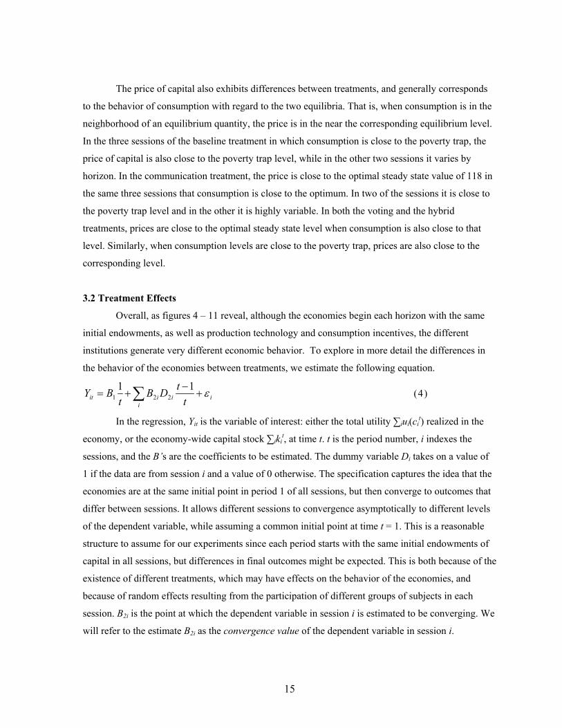
3.2 Treatment Effects

Overall, as figures 4 – 11 reveal, although the economies begin each horizon with the same

initial endowments, as well as production technology and consumption incentives, the different

institutions generate very different economic behavior. To explore in more detail the differences in

the behavior of the economies between treatments, we estimate the following equation.

∑ +−

+=i

iiiit ttDB

tBY ε11

221 (4)

In the regression, Yit is the variable of interest: either the total utility ∑iui(cit) realized in the

economy, or the economy-wide capital stock ∑ikit, at time t. t is the period number, i indexes the

sessions, and the B’s are the coefficients to be estimated. The dummy variable Di takes on a value of

1 if the data are from session i and a value of 0 otherwise. The specification captures the idea that the

economies are at the same initial point in period 1 of all sessions, but then converge to outcomes that

differ between sessions. It allows different sessions to convergence asymptotically to different levels

of the dependent variable, while assuming a common initial point at time t = 1. This is a reasonable

structure to assume for our experiments since each period starts with the same initial endowments of

capital in all sessions, but differences in final outcomes might be expected. This is both because of the

existence of different treatments, which may have effects on the behavior of the economies, and

because of random effects resulting from the participation of different groups of subjects in each

session. Β2i is the point at which the dependent variable in session i is estimated to be converging. We

will refer to the estimate Β2i as the convergence value of the dependent variable in session i.

15

Tables 2 and 3 contain the estimation results for the dependent variables of total capital in the

economy and total welfare of the economy, respectively. Conducting a similar analysis on the

variables price of capital and total output, yields qualitatively similar results with regard to the

relationship of the data to the two equilibria.

[Insert tables 2 and 3 about here]

There are several patterns in the data that emerge from this analysis, confirming the visual

impression from the graphs. The first is that there is a strong tendency for the data in the baseline

treatment for convergence to one of the equilibria, and this is usually the poverty trap. None of the

five convergence values for the level of capital is both significantly different from the optimal

equilibrium level of 45 and from the inferior equilibrium of 9. Four of the five are not significantly

different from the poverty trap level of 9 at the 5% level. The same pattern holds for the welfare of

the economy. Four of five economies have convergence values that are not different at the 5% level

of significance from the poverty trap level of 5856, and one converges to a level not different from

the optimal steady state level of 18060. Thus hypothesis 1 is supported in our data. The baseline

treatment converges to the poverty trap, representing a welfare loss of over two-thirds of the welfare

that would be attained at the optimal equilibrium.

The second pattern is that the economies in the communication treatment exhibit variable

outcomes between sessions, but each estimated coefficient for a session has a very small standard

error. This indicates a strong tendency toward convergence to some level of capital stock within a

session, but with considerable heterogeneity between sessions. Capital stock in one of the sessions

converges to a level not significantly different from the poverty trap. The significance of the

differences between the data and the equilibrium levels is due in part to the very small standard

errors. With regard to welfare, three of the six sessions converge to levels not different from the

poverty trap level, and two of the sessions converge to levels not different from the optimal

equilibrium.

The voting treatment estimates have much higher variance than those in the baseline and the

communication treatments. This suggests that the voting treatment generates larger fluctuations from

one period to another, even asymptotically. Capital stock levels in three of the five sessions converge

to levels that are different from the optimal equilibrium, and in one session to a level not different

from the poverty trap. The estimated convergence values of welfare all lie between the values of the

two equilibria, and are characterized by large standard errors, reflecting the large changes in capital

16

stock and consumption from one period to the next. Two sessions attain values not significantly

different from the optimal equilibrium, while two others reach levels not different from the poverty

trap. This suggests that conflict often occurs in the voting process. Indeed, some proposals reflect a

preference for a high level of current consumption rather than for building up sufficient capital to

surpass the threshold, and the majority will at times vote in favor of such proposals. Individual

behavior in the voting treatment is considered in more detail in subsections 3.5 and 3.6.

Finally, the hybrid treatment estimates on average reflect capital stock levels that are higher

than in the other treatments. Two sessions attain levels not different from the optimal equilibrium, but

in contrast to all of the other treatments, all convergence values are significantly different from the

poverty trap value. A similar result applies to total welfare. All convergence values exceed the

poverty trap level and the difference is significant. The standard errors are typically larger than under

the baseline and the communication treatments, but are similar to those in the voting treatment.

Thus it appears that the hybrid treatment is the most conducive to allowing the economy to

surpass the threshold and exit the poverty trap. The voting process, present in the voting and the

hybrid treatments, in which the majority dictates the consumption and investment decisions of the

economy, appears to solve the coordination problem of how to avoid the inferior equilibrium.

However, the voting process also distorts the economies in a manner that introduces additional

variance from one period to the next, making the behavior of the economy less stable than under the

systems in which individuals make their own consumption and investment decisions. On the other

hand, while communication imposes no distortion from the imposition of the majority will on the

minority, it is not fully effective as a coordinating mechanism for exiting the poverty trap, perhaps

because it is not completely effective in eliminating strategic uncertainty.

We now consider the effects of the different treatments on the values obtained of two

aggregate measures of economic activity, total output of the economy and total welfare, and we

evaluate hypotheses 2 – 4. To do so, we conduct Mann-Whitney rank sum tests of the differences in

both output and welfare between treatments, maintaining the conservative assumption that each

session is a unit of observation. The total output of the economy is equal to the value of F(Kt) =

Σifi(kit). the economy realizes in period t. The total welfare in period t is defined as U(Ct) = Σiui(ci

t).

To normalize the measure the total output or welfare in the economy to achieve comparability

between sessions containing a different number of periods, the average observed value of the variable

by period is used. This average is calculated using two different weighting schemes, period and

horizon weighting. Under period weighting, each period of activity receives equal weight in the

calculation of the average, regardless of the length of the horizon that includes the period. Under

17

horizon weighting, each horizon receives equal weight. To calculate the average value of a variable in

a session under horizon weighting, we calculate the average value by period within a horizon, and

then calculate the average of the resulting horizon averages. The result of this calculation is the

average value of the variable for the session.

With regard to the output of the economy, under period weighting, we fail to reject the

hypothesis that the baseline and communication treatments are different at the 5% level (z = 1.095, p

= .273). However, we are able to reject the hypothesis that the baseline and voting treatments yield

the same output (z = 2.193, p = .028), with the addition of the voting institution increasing output.

There is no difference between the communication and the hybrid treatments (z = .913, p = .333), or

between the voting and the hybrid treatments (z = 1.149, p = .251). We also reject the hypothesis that

output is equal in the baseline and the hybrid treatments (z = 2.611, p = .009 ) Under horizon

weighting the same results are obtained. We fail to reject the hypotheses that the baseline and the

communication (z = 1.095, p = .273), the communication and hybrid (z = .548, p = .583), and the

voting and hybrid treatments (z = .522, p = 602) yield identical output. However, we find that voting

leads to higher output than under the baseline treatment, rejecting the null hypothesis of no difference

(z = 2.193, p = .028). We also reject the hypothesis of equality of output in the baseline and the hybrid

treatments under horizon weighting (z = 2.611, p = .009).

Thus we support hypothesis 3a, but fail to support 2a, 2b, and 3b. Voting has a positive

impact on output when there is no free expression, but its marginal impact is attenuated when free

expression exists. It appears that there is some redundancy in the two instruments, although the

application of both together achieves outcomes that are no worse than each instrument separately.

With regard to overall welfare, we find similar patterns. The only treatment differences that

are significant at the 5% level are those between the baseline and voting treatments and the baseline

and hybrid treatments. This is true under both the period and the horizon weighting systems. Thus the

data provide support for hypothesis 4d, but do not support 4a-c. The voting process increases total

output and welfare significantly over the baseline treatment, whether or not the process exists alone or

in conjunction with free expression between agents. The next five sections present an exploratory

analysis of empirical patterns that have appeared in our data.

3.3 Inequality and Sources of Inefficiency

The distribution of earnings in the experiment is of potential interest. Our study was not

intended to study inequality directly, and has no explicit mechanism of taxes and transfers that can

reduce or increase inequality. Any differences in equality that arise here are presumably due to the

18

interaction of behavioral phenomena and the different institutions rather than a conscious effort to

apply equity considerations. We consider two questions in this subsection. The first is whether

inequality differs between treatments. Although average earnings may be greater under one treatment

than another, the improvement may come at a cost of increased inequality. The second question is

whether earnings are more equal than at the optimum, that is, whether departures from maximal

earnings at the aggregate level are consistent with a tendency to split earnings more equally and thus

there exists a type of equity/efficiency tradeoff. This may be due to general properties of the

convergence process of the markets (see Smith and Williams, 1982) where rents may be split more

equally between participants while a market is in disequilibrium than in a competitive equilibrium. In

treatments with communication and voting, the reduction in inequality may be due to an explicit

agreement between agents to share rents or to the existence of proposals that attempt to redistribute

wealth between agents. While there are many possible measures of inequality, we choose the

following, which is a version of a measure of inequality due to Theil (1967):

½((1/(Iit) *(1/n*(Ii

t)2)1/2)2 (4)

where Iit = + m)( i

ti cv i1

t – mi0t. Ii

t is proportional to the dollar earnings obtained by the

subject in the role of individual i and thus is a measure of income for a period. The average values

and standard deviations (assuming that each session is an observation) of the measure are 1.18 and

2.34 in the baseline treatment, and .95 and 1.28 in the communication treatment. The mean in the

voting treatment is .86 with a standard deviation 1.28. In the hybrid treatment, the mean is .84 with a

standard deviation of 1.44. A Mann-Whitney rank sum test, using the average inequality in each

session as an observation (5 to 6 observations by treatment) indicates that none of the differences

between treatments are significant. The communication, voting, and hybrid processes achieve higher

welfare than the baseline treatment (though the effect is not significant for communication) without

an increase in inequality. Each treatment generates greater inequality than in the optimal steady state,

in which Ii = .49. However, within each system, more equality of earnings is associated with lower

total earnings in the economy. This pattern, along with the absence of strong differences between

treatments, can be seen in figure 12. In the figure, each data point represents one period.

[Figure 12: About Here]

19

There are three types of allocative inefficiency that can appear in the experiment. The first is

what we will call the output gap, a lower actual production level that the highest that could be

achieved with the capital that currently resides in the economy. An output gap occurs because the

capital at the end of the period is allocated among agents in a manner other than to the individuals

with the highest marginal products for capital. The output gap is calculated as (F*(Σikit) - Σifo(ki

t))/

F*(Σikit), where F*(Σiki

t) is the maximum possible production possible with capital stock kit and

Σifo(kit) is the actual production observed. The output gap is remarkably constant across treatments

and sessions. It equals on average 6.59%, 6.37%, 6.45%, and 7.26% in the baseline, voting,

communication and hybrid treatments, respectively. The output gap averages between 2.8% and 9.4%

in every session. Thus, none of our treatments reduce the output gap from the level in the baseline

treatment.

A second type of inefficiency is consumption inefficiency. The value of a given amount of

aggregate consumption is maximized when the units are allocated to individuals in order of their

marginal utility of consumption. If a unit can be transferred from an individual to another who has a

higher marginal utility for the unit, the original allocation was inefficient. The consumption

inefficiency can be measured as the ratio (U(Ct) – Σvio(ci

t))/U(Ct), where Σvio(ci

t) is the actual total

value of consumption that individuals have achieved in period t, and U(Ct) is the optimal level. This

loss is greater in the communication and the hybrid treatments (7.65% and 7.16% respectively), than

in the baseline and voting treatments, where it equals 3.90% and 5.22% respectively. The relatively

good performance of the baseline treatment on this measure may be due to the stronger tendency for

convergence to competitive equilibrium in the baseline than in the other treatments. The stability that

accompanies the equilibrium makes it easier to discern the price of capital and therefore to correctly

apply the optimal decision rule of consuming until the marginal utility of consumption equals the

price of capital. It is rather surprising that the average level of consumption inefficiency is lower

under voting than other treatments, since individuals are not completely free to choose their own

consumption levels, but rather are required to consume the quantity allotted to them under the

winning proposal.

The third kind of inefficiency is dynamic inefficiency, which results from suboptimal

allocations to investment and consumption. Let V(Kt) be the value of the capital stock in period t,

assuming that the economy behaves like a social planner, making optimal decisions from period t

onward. The market value of a unit of capital in period t under this assumption can be calculated for

each current level of capital stock. The market value in period t is equal to the marginal utility of

consumption in period t along the economy’s optimal trajectory. Let V(K*t) be the value of the

20

optimal quantity of capital stock given the current level of output (Ct-1 + Kt) and V(Kt) be the actual

value of the total level of capital generated from the individual agents’ actual choices. The level of

dynamic inefficiency in period t is defined as defined as (V(K*t) - V(Kt))/V(K*

t). This measure shows

considerable differences between treatments. In the baseline treatments, the level of dynamic

inefficiency averages 21.99%. In the voting and communication treatments, the inefficiency is

12.81% and 12.27%, respectively. In the hybrid treatment, the average value of the measure is 5.01%.

The hybrid treatment has the lowest dynamic efficiency, and this effect appears to be due to its

greater success in escaping the poverty trap compared to the other treatments. The chat-room

transcripts in both the communication and the hybrid treatments contain no attempts to reduce the

output gap or consumption inefficiency.

3.3 Market behavior

We now consider the behavior of the markets for output in the economies. We focus on the

relationship between the price and the quantity of output and the efficiency of the pricing mechanism.

If the price system is functioning, it should reflect the scarcity of output in the economy, resulting

from demand for both consumption and investment purposes. Figure 13 shows the relationship

between price and total output in the economy. The line drawn is the linear function that minimizes

the squared sum of deviations between the observed and the predicted price-quantity combinations,

and the line can be interpreted as an approximation of the revealed demand function for output in the

economy.

The poverty trap equilibrium levels of price and output are 334 yen (units of experimental

currency) and 25 units respectively. In the optimal equilibrium, the price equals 118 and the quantity

of output is 115. As can be seen from the graphs, demand is downward sloping in each of the

treatments. Evaluated at the optimal equilibrium quantity of 115, inverse demand equals 149 and 122

in the baseline and communication treatments, respectively, close to the equilibrium price of 118, and

lying within the 95% confidence interval for the predicted value. However, under the voting and the

hybrid treatments, the inverse demands at a quantity of 115 are 178 and 4, respectively, which are

significantly different from equilibrium levels. In the inferior equilibrium, there are 25 units

demanded at a price of 334. Evaluating the estimated inverse demand function for output at a quantity

of 25, we get values of 365, 299, and 300 in the baseline, communication, and voting treatments,

which are not significantly different at the 5% level from equilibrium levels. However, the value in

the hybrid treatments is 243, which is rather distant and significantly different from the equilibrium

level. Thus market demand behaves in a manner more consistent with equilibrium patterns in the

21

baseline and communication treatments, in which the market is not subject to the repeated shocks to

output quantity that results from the voting process.

[Figure 13: About Here]

We can also consider whether market prices satisfy rational expectations. For each level of

aggregate output, it is possible to calculate the value for each unit of output assuming the entire

economy behaves optimally from the current period onward. This can be calculated in the following

manner. Suppose the economy from period t onward is directed by a benevolent social planner

choosing aggregate levels and individual allocations of capital and consumption to maximize total

welfare. Then there is an optimal sequence of capital stock levels from period t on, and thus an

optimal amount of capital stock for the economy to hold for period t+1. The market value of a unit of

capital under this assumption can be calculated for each current level of capital stock. The diamond-

shaped markers in figure 13 illustrate these prices given the actual capital stock in each period t for

each treatment. The figure reveals that the actual price quantity combinations observed are close to

those under rational expectations.

3.4. How do the economies avoid the poverty trap?

The market mechanism that we have introduced in our economies appears to be an effective

institutional structure for reaching a competitive equilibrium, provided that the economy is in the

basin of attraction of the equilibrium. However, an economy with multiple equilibria poses an

additional challenge in that the market. To operate efficiently, the market must not only locate an

equilibrium, but must select the optimum from a set of equilibria.

In the baseline treatment, the difficulty of this challenge is apparent. The market alone, in

conjunction with an initial endowment below the threshold level of capital stock, is only able to

surpass the threshold in a small minority of instances. However, the additional institutions of

communication and voting increase the likelihood that the economy surpasses the threshold. When

both are applied together, in the hybrid treatment, the economy surpasses the threshold with some

consistency in every session. In this subsection, we explore the manner in which the economy

successfully surpasses the threshold in the various treatments we have studied.

In the baseline treatment there were only two episodes in which the capital stock of the

economy surpassed the threshold level of 31. One instance occurred in the fifth horizon of session

Caltech2, which lasted three periods. It surpassed the threshold in period 2 and remained above the

22

threshold for the remainder of the horizon. It was able to cross the threshold because agent 1, the

agent with the most efficient production function, purchased a number of units in period 2 to have a

final period holding of 28, which required the other four people to hold a total of three units for the

threshold to be surpassed. The other episode occurred in the second period of the first horizon of

session Emory3, and was also essentially a single-handed effort. In this period, agent 3 invested and

purchased a large amount of capital so that he held 16 at the end of the period. Even though no other

agent held more than six units, the economy-wide level reached 32. However, this behavior was

profitable for agent 3, and was not attempted again in the session. Thus, when the economy

successfully exited the poverty trap in the baseline treatment, it was not through coordination but

rather because one individual reduced his own consumption by a sufficient amount to enable the

economy to exit the poverty trap.

[Figure 14: About Here]

In the communication treatment, the exchange of messages facilitates coordination and

thereby makes it more likely that the threshold is surpassed. However, it does not guarantee that the

economy escapes the poverty trap. In two sessions, the economy failed to surpass the threshold. In the

periods in which the threshold was surpassed, communication always followed a specific pattern. One

player would suggest that players not consume at all or consume very small quantities in the current

period, and two or more players would indicate agreement. Then after successfully passing the

threshold, the next period was characterized by acknowledgement of the successful coordination.

Figure 14 displays, for every period of the communication and the hybrid treatments, the number of

individuals who either proposed or agreed that the group should try to coordinate their decisions to

exceed the threshold, along with the capital stock held after the communication occurred, the market

operated, and consumption took place. The figure shows that when the economy was below the

threshold, majority agreement to coordinate was always necessary for the economy to surpass the

threshold. In the two sessions in which the threshold was never surpassed, there was no expression of

majority support for attempting to surpass it at any time.

Two examples of typical dialogue in the period in which the threshold was surpassed for the

first time in a session in the communication treatment are presented below.

Example 1: Horizon 2, Communication treatment, Session EmoryC1

Period 1

23

(player 4)>HOLD K for a round (player 2)>once again...lets keep all our k...nobody consume this round (player 4)>is that good player 1 and 5 (player 1)>we say that every round and no body does it (player 5)>we only have a few min. left (player 4)>just do it for the first round and we all will have a lot more to use Period 2: (player 4)>SEE! (player 3)>good work (player 2)>wanna do it again? (player 3)>let's let it keep growing

Example 2, Horizon 3, Communication, Session EmoryC2

Period 1:

(player 5)>NOBODY CONSUME (player 1)>DONT CONSUME (player 4)>lets get this show on the road...move quick (player 5)>JUST THE FIRST ROUND, ITS WELL WORTH IT (player 1)>lose a lil...make a lot (player 3)>HOW (player 2)>by not consuming Period 2: (player 1)>GOOD JOB (player 4)>well done (player 5)>THAT A WAY TO DO IT

In the hybrid treatment, the patterns of communication do not typically follow the same

pattern. Indeed, in only six of fifteen instances in which the threshold was surpassed and only two

instances when it was surpassed the first time in a session, was there agreement from a majority that

players should be investing more. The voting process on its own provides the device to coordinate

decisions to surpass the threshold. Expression of a consensus on the need to overcome the threshold is

not required when the voting process is available, since one proposer, along with majority approval

after the proposal is submitted, is sufficient to coordinate the economy’s activity. The majority does

not have to express a desire to invest more for the coordination problem to be solved. There is no

24

problem of strategic uncertainty. Indeed, in this treatment, there were often expressions of a desire to

consume a large quantity in the current period rather than attempting to exceed the threshold.

In the voting and hybrid treatments, when the economy was below the threshold and there

were two proposals to bring it over the threshold, there was a consistent pattern of behavior. In only

one instance out of 10 in the voting treatment did the proposal that specified holding more capital

than the other defeat the one with less capital proposed. This one instance was a pair of proposals in

which one alternative proposing an aggregate level of capital stock of 32 defeated one proposing 31.

In none of the 8 instances in which the threshold was crossed in the hybrid treatment did the proposal

with the higher capital stock win. The winner was always 31 in these situations in the hybrid

treatment.

Submitting a proposal with aggregate capital stock above the threshold while the economy

was below it, did not guarantee that the economy would surpass the threshold. When the economy

was below the threshold and exactly one proposal exceeded the threshold, it won its vote in 12 of 21

(57.1%) instances in the voting treatment. This increased to 9 of 11 (81.8%) instances in the hybrid

treatment. In the baseline and the communication treatments, there was not a single instance in which

an economy surpassed the threshold and later fell below it in the same horizon. On the other hand

there two such instances in the voting treatment and two more in the hybrid treatment. This may be

because, in contrast to the communication treatment, it may not be common knowledge that

surpassing the threshold is desirable.

3.5. Voter and proposer behavior: What is proposed and what do people vote for?

In this subsection we explore voters’ choices and consider whether there exist any strong patterns of

voter behavior. We ask first whether or not agents tended to vote rationally. In each period, we can

calculate a myopically optimal level of consumption, which if followed, would reflect a plausible

level of rationality. Because an individual can allocate output to either capital or consumption, at an

optimum in which a positive quantity of output is assigned to each use, the marginal value of each use

must be equal. Therefore, it is optimal for an individual to consume until the marginal utility of

consumption equals the future price of capital. To enable calculation of the expected price of capital

in the next period, we suppose that the expected future price of capital is equal to the average price in

the current period. This seems to be a reasonable supposition for the beliefs of individuals in the

experiment. We consider whether individuals vote for the proposal that yields them a value of

consumption closer to the optimum compared to the other proposal. Because the utility of an

individual is concave in the quantity of own consumption chosen given fixed prices and own output,

25

proposals specifying a consumption level closer to an individual’s optimum will tend to yield higher

total earnings.

The data are displayed in table 4. As can be seen from the table, we find no evidence of a

tendency to vote for the proposal closer to one’s optimum. In each of the ten sessions of the voting

and hybrid treatments, individuals vote for the alternative that is farther from their optimum a

majority of the time. Rather than vote for the proposal closer to the optimum, there is a strong general

tendency to vote for the alternative that gives the voting individual a greater level of consumption

from among the two choices. These data are given in table 5. In nine of ten sessions at least as many

votes are in favor of the alternative with greater own consumption. Overall, when a voter chooses

between proposals that differ in terms of his own consumption, he votes for the proposal yielding

greater own consumption in 62.1% of possible instances in the voting treatment, and in 61.1% of

instances in the hybrid treatment.

[Tables 4 – 6: About Here]

Exploration of the proposal data shows a strong tendency for proposers to submit proposals

that yield themselves more consumption than at the myopic optimum. Compared to the myopic

optimum, agents propose more consumption for themselves an average of 70.4% of the time in the

voting treatment and 69.4% of the time in the hybrid treatment. The data by session is displayed in

table 6, and shows that in every session, a majority of submitted proposals yield the proposer more

consumption than his optimal choice.

Another interesting pattern is that when the economy is below the threshold, only 28.6%

percent of the proposals in the voting treatment would bring the economy up over the threshold. Thus,

the voting process did not necessarily lead immediately to effective collective behavior. In the hybrid

treatment, however, this percentage increases to 61.4%. The communication between members of the

group appears to help individuals to formulate proposals that are better for the group. Once above the

threshold, the vast majority of proposals would keep capital stock over the threshold in both the

voting and the hybrid treatments.

4. Conclusion In this paper we introduce a laboratory methodology for studying the effect of institutions on

economic growth. Our first conclusion is that is feasible and productive to do so. Experiments allow

the actual behavior of the economy to be compared with the optimum path the economy could

26

achieve. They permit a focus on economies with specific characteristics, such as those with multiple

equilibria. Institutional structures can be compared in settings in which all environmental variables

can be held constant. The direct and interaction effects of the decision biases, trembling hand errors,

strategic uncertainty, and cooperative motives that influence human behavior and that are not

captured in traditional macroeconomic models can appear in our economies. The experiment allows

observation of such behavioral elements as they interact with different institutions and generate

patterns of behavior that have implications on output and welfare of the economy. Behavioral

phenomena that might cause an economy to operate below its optimum might be identified. We view

this study as a first step, and we believe that there is great potential in bringing experimental

economic methods to bear on issues of macroeconomic policy and economic development.

In our study, we observe clear effects of institutions on income and on the ability to avoid a

poverty trap. We advanced several hypotheses that were, for the most part, consistent with the data.

Then economies of the baseline treatment tend to converge to the poverty trap of the economy, which

is not a surprising results since the parameters were chosen to make this a likely outcome for the

baseline treatment. The data from the baseline treatment indicate that while a centrally organized

market institution reliably will reach a competitive equilibrium, additional institutions may be

required to help select the optimal from among several equilibria. We identify two institutions,

communication and voting, which when applied together, are sufficient to enable the economy to

extricate itself from the poverty trap.

Both the availability of communication, a highly stylized version of free expression, and our

voting process, a highly stylized democratic process, improve output and welfare over the level

achieved in the baseline treatment, and the effect is significant in the case of the voting process. The

task faced in our economies with multiple equilibria is a specific type of coordination of activity

among agents. The communication treatment promotes, but does not guarantee that coordination

occurs, presumably because it reduces strategic uncertainty about voters’ decisions. It increases the

probability that the economy will exit the poverty trap, and in cases where this is successful, the

economy then tends to move in the direction of the optimal equilibrium. There is little variance in

outcomes from one period to the next once the threshold has been crossed, as the prices in the market

help guide the economy toward its optimum.

The voting process also increases the likelihood that the poverty trap is escaped. Although the

voting process is characterized by significantly higher output and welfare than the baseline treatment,

the variance of outcomes and the fluctuations from one period to the next are greater. When the

communication and voting process are both in effect in the hybrid treatment, output and welfare are

27

also significantly greater than in the baseline treatment. The hybrid is the only treatment, in which the

economy surpasses the poverty trap in every session. Thus, we find that a particular implementation

of “democracy” promotes growth and welfare in our economies, and this is effect is more reliable

when citizens of the economies can engage in free expression.

Of course, our inferences are specific to economies with the particular structure we have

studied. As with theoretical modeling, both the environment and the institutions are very simple

compared to those that are naturally occurring. The level of generality of any empirical patterns

observed in this or any other study of this type must be determined with an accumulation of evidence.

No one study can yield conclusive results. The structure here was intentionally chosen to have the

structure of a well-known theoretical model. However, it is straightforward to add features of

macroeconomies that are of interest to economists, such as allowing for endogenous growth, multiple

interacting economies with an international structure, multiple sectors in the economy, and a wider

array of government policies options, both fiscal and monetary. Institutions that are successful at

producing wealth in one environment can be implemented in another to test their robustness. We may

find that certain institutions are more suitable for economies with certain endowment levels or

production technologies. For example, in an economy with a single rational expectations competitive

equilibrium, decentralized markets alone may be very effective in guiding economic activity to close

to its optimum. However, as our data here suggests, in an economy with multiple equilibria, the same

minimal institutional structure may lead to a suboptimal equilibrium, and supplemental institutions

may be required to select optimal equilibria. In principle, using experimental methods, different

political systems such as dictatorship, indirect democracy, socialism, and anarchy can be

implemented, their performance measured, and their properties studied. Auxiliary institutions such as

an independent central bank, financial markets and can be added and their effect in conjunction with

other institutions and behavioral factors studied. Finally, new institutions that theory and economic

intuition suggest may promote economic growth can be designed, tested and refined in the laboratory.

References Acemoglu, Daron, Simon Johnson and James Robinson, “The Colonial Origins of Comparative

Development: An Empirical Investigation,” American Economic Review, December 2001, 91(5), 1369-1401

Azariadis, Costas and Allan Drazen, “Threshold Externalities in Economic Development,” Quarterly Journal of Economics, May 1990, 105(2), 501-26.

Azariadis, Costas, Intertemporal Macroeconomics, Cambridge, MA: Blackwell, 1993.

28

Banerjee, Abhijit,Fr Dilip Mookherjee, Kaivan Munshim and Debraj Ray, “Inequality, Control Rights, and Rent Seeking: Sugar Cooperatives in Maharashtra,” Journal of Political Economy, 2001, 109, 138-90.

Barro, Robert J. and Xavier Sala-i-Martin, Economic Growth, New York: McGraw-Hill, 1995. Barro, Robert J., Determinants of Economic Growth: A Cross-Country Empirical Study, MIT Press,

1997. Baumol, William J., “Productivity Growth, Convergence, and Welfare: What the Long-Run Data

Show,” American Economic Review, 76(5), December 1986, 1072-85. Camerer, Colin and Keith Weigelt, “Convergence in Experimental Double Auctions for

Stochastically Lived Assets,” in D. Friedman and J. Rust, eds., The Double Auction Market: Institutions, Theories, and Evidence, New York: Addison-Wesley, 1993, 355-96.

Cass, David, “Optimal Growth in an Aggregative Model of Capital Accumulation,” Review of Economic Studies, July 1965, 32(3), 233-40.

Cooper, Russell, “Estimation and Identification of Structural Parameters in the Presence of Multiple Equilibria”, working paper, Boston University, 2002.

Durlauf, Steven and Danny Quah, “The New Empirics of Economic Growth,” in John Taylor and Michael Woodford, eds., Handbook of Macroeconomics, Amsterdam, New York and Oxford: Elsevier Science, North-Holland, 1999, 235-308.

Galor, Oded and Joseph Zeira, “Income Distribution and Macroeconomics,” Review of Economic Studies, January 1993, 60(1), 35-52.

Islam, Nazrul, “What Have We Learned from the Convergence Debate? A Review of the Convergence Literature,” Journal of Economic Surveys, July 2003, 17 (3), 309-362.

Knack, S., and P. Keefer, “Does Social Capital Have an Economic Payoff? A Cross-Country Investigation”, Quarterly Journal of Economics, 112, 1251-1288.

Koopmans, Tjalling C., “On the Concept of Optimal Economic Growth,” in Pontifical Academy of Sciences, The Econometric Approach to Development Planning, Amsterdam: North-Holland, 1965, 255-87.

Lei, Vivian and Charles Noussair, “An Experimental Test of an Optimal Growth Model”, American Economic Review, Vol. 92, no 3, June 2002, pages 549-570.

Lei, Vivian and Charles Noussair, “Equilibrium Selection in an Experimental Macroeconomy”, working paper, Emory University, 2003

Murphy, Kevin M., Andrei Shleifer, and Robert W. Vishny, “Industrialization and the Big Push,” Quarterly Journal of Economics, May 1989, 106(2), 503-530.

Noussair, Charles N. and Kenneth Matheny, “An Experimental Study of Decisions in Dynamic Optimization Problems,” Economic Theory, March 2000, 15(2), 389-419.

Noussair, Charles, Charles Plott, and Raymond Riezman , “An Experimental Investigation of the Patterns of International Trade”, with Charles Plott and Raymond Riezman, American Economic Review, June 1995, pages 462-491.

Plott, Charles and Glen George, “Marshallian vs. Walrasian Stability in an Experimental Market,” Economic Journal, May 1992, 102, 437-460.

Ramsey, Frank P., “A Mathematical Theory of Saving,” Economic Journal, December 1928, 38, 543-59.

Rosenstein-Rodan, Paul, “Problems of Industrialization of Easter and Southeastern Europe,” Economic Journal, 53, June-September 1943, 202-211.

Sachs, Jeffrey and Andrew Warner (1995), “Economic Reform and the Process of Global Integration,” Brookings Papers on Economic Activity, 1995:I, 1-118

Smith, Vernon “An Experimental Study of Competitive Market Behavior,” Journal of Political Economy, 1962, 70, 111-137.

29

Smith, Vernon and Arlington Williams (1982), “The Effect of Rent Asymmetries in Experimental Double Auction Markets”, Journal of Economic Behavior and Organization, 3(1), 99-116.

Temple, Jonathan, “The New Growth Evidence,” Journal of Economic Literature, March 1999, 37(1), 112-56. Theil, H., 1967, Economics and Information Theory, North Holland, Amsterdam.

30

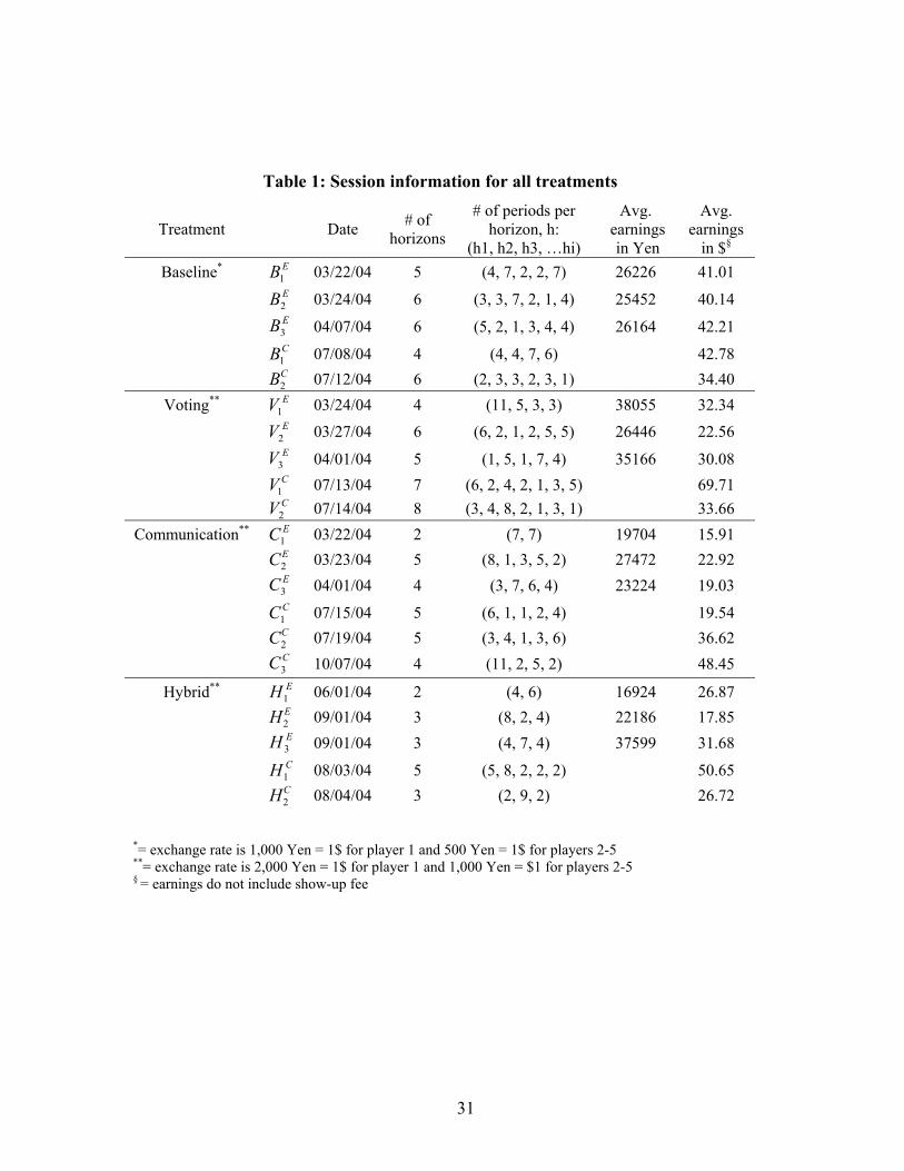
Table 1: Session information for all treatments

Treatment Date # of horizons

# of periods per horizon, h:

(h1, h2, h3, …hi)

Avg. earnings in Yen

Avg. earnings

in $§ Baseline* EB1 03/22/04 5 (4, 7, 2, 2, 7) 26226 41.01

EB2 03/24/04 6 (3, 3, 7, 2, 1, 4) 25452 40.14

EB3 04/07/04 6 (5, 2, 1, 3, 4, 4) 26164 42.21

CB1C

07/08/04 4 (4, 4, 7, 6) 42.78 B2 07/12/04 6 (2, 3, 3, 2, 3, 1) 34.40

Voting** EV1 03/24/04 4 (11, 5, 3, 3) 38055 32.34

EV2 03/27/04 6 (6, 2, 1, 2, 5, 5) 26446 22.56

EV3C

04/01/04 5 (1, 5, 1, 7, 4) 35166 30.08 V1

C 07/13/04 7 (6, 2, 4, 2, 1, 3, 5) 69.71

V2 07/14/04 8 (3, 4, 8, 2, 1, 3, 1) 33.66 Communication** EC1 03/22/04 2 (7, 7) 19704 15.91

C2E 03/23/04 5 (8, 1, 3, 5, 2) 27472 22.92

EC3 04/01/04 4 (3, 7, 6, 4) 23224 19.03

CC1C

07/15/04 5 (6, 1, 1, 2, 4) 19.54 C2 07/19/04 5 (3, 4, 1, 3, 6) 36.62 CC3 10/07/04 4 (11, 2, 5, 2) 48.45

Hybrid** EH1 06/01/04 2 (4, 6) 16924 26.87 H2

E

E 09/01/04 3 (8, 2, 4) 22186 17.85 H3

C

09/01/04 3 (4, 7, 4) 37599 31.68

H1C

08/03/04 5 (5, 8, 2, 2, 2) 50.65 H2 08/04/04 3 (2, 9, 2) 26.72

*= exchange rate is 1,000 Yen = 1$ for player 1 and 500 Yen = 1$ for players 2-5 **= exchange rate is 2,000 Yen = 1$ for player 1 and 1,000 Yen = $1 for players 2-5 § = earnings do not include show-up fee

31

Table 2: Convergence Regression Results for Capital

N of observations = 521; R2=0.5225; § = surpassed the threshold level of K Optimal SS capital = 45, Poverty trap capital = 9

At the5% level, significantly different from K level Coefficient Std Error

Optimal SS Poverty trap Baseline EB1 7.124851 1.83002 no

EB2 5.784205 1.855012 no

EB3 20.805 9.165125 no

CB1C

6.923799 1.903858 no

B2 32.56667 9.932392 § no

Voting EV1 48.41585 6.730324 § no

EV2 9.319982 1.283418 no

EV3 61.67496 10.51112 § no

V1C

C 36.68258 6.307952 § no

V2 33.39724 3.475891 §

Communication EC1 47.93213 14.02123 § no

C2E 24.06306 4.840741

EC3 6.436223 1.04832

CC1C

7.791051 2.685231 no

C2 58.5265 2.688141 §

CC3 57.30678 1.356395 §

Hybrid EH1 37.17351 3.96 § no

H2E 47.58473 14.87 § no

EH3 79.47027 6.700127 §

CH1C

34.12632 2.140628 §

H2 33.9695 3.51596 §

32

Table 3: Convergence Regression Results for Welfare

N of observations = 521; R2=0.6404; § = surpassed the threshold level of K Optimal SS welfare = 18060, Poverty trap welfare = 5856

At the 5% level, significantly different from K level Coefficient Std Error

Optimal SS Poverty trap Baseline EB1 5478.777 339.977 no

EB2 5601.239 807.5723 no

EB3 10838.32 2196.931

CB1 5054.917 383.8095

B2C 9389.186 2801.525 § no

Voting EV1 11023.11 1769.569 §

EV2 6067.609 351.3269 no

EV3 14761.31 2283.481 § no

V1C 11977.68 2710.068 §

V2C 8938.886 2317.232 § no

Communication EC1 9148.591 2610.409 § no

C2E 9654.752 2081.423 no

EC3 5646.167 446.1572 no

CC1C

4175.423 586.9262

C2 17664.82 1592.376 § no

CC3 19539.32 754.7449 § no

Hybrid EH1 11879.98 2826.926 §

H2E 11584.68 1083.541 §

EH3 15822.39 1660.017 § no

CH1 20674.43 1326.051 §

H2C 11857.13 2273.16 §

33

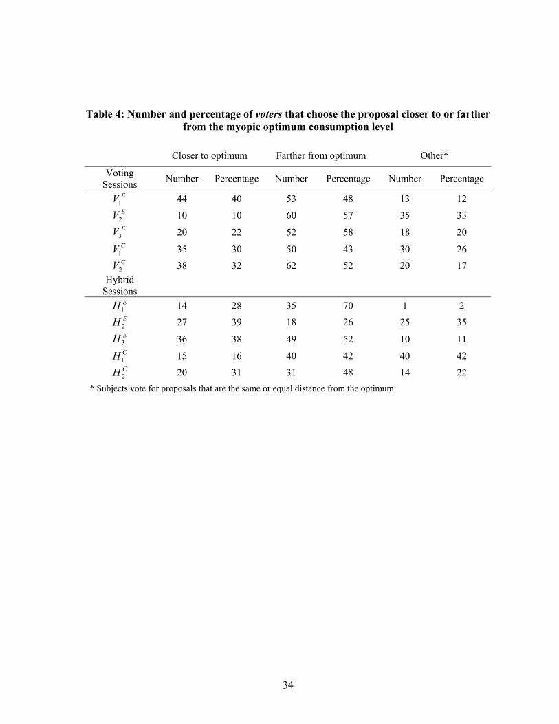
Table 4: Number and percentage of voters that choose the proposal closer to or farther

from the myopic optimum consumption level

Closer to optimum Farther from optimum Other*

Voting Sessions Number Percentage Number Percentage Number Percentage

EV1 44 40 53 48 13 12 EV2 10 10 60 57 35 33 EV3 20 22 52 58 18 20 CV1 35 30 50 43 30 26 CV2 38 32 62 52 20 17

Hybrid Sessions

EH1 14 28 35 70 1 2 EH 2 27 39 18 26 25 35 EH3 36 38 49 52 10 11 CH1 15 16 40 42 40 42 CH 2 20 31 31 48 14 22

* Subjects vote for proposals that are the same or equal distance from the optimum

34

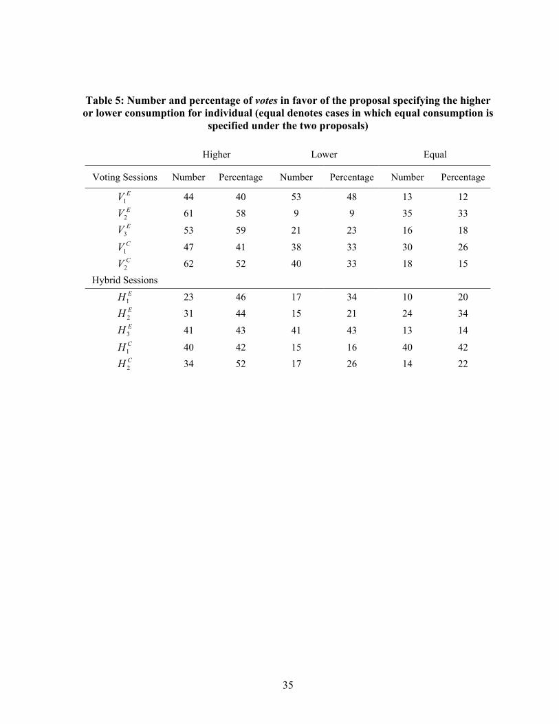
Table 5: Number and percentage of votes in favor of the proposal specifying the higher or lower consumption for individual (equal denotes cases in which equal consumption is

specified under the two proposals)

Higher Lower Equal

Voting Sessions Number Percentage Number Percentage Number Percentage EV1 44 40 53 48 13 12 EV2 61 58 9 9 35 33 EV3 53 59 21 23 16 18 CV1 47 41 38 33 30 26 CV2 62 52 40 33 18 15

Hybrid Sessions EH1 23 46 17 34 10 20 EH 2 31 44 15 21 24 34 EH3 41 43 41 43 13 14 CH1 40 42 15 16 40 42 CH 2 34 52 17 26 14 22

35

Table 6: Number and percentage of proposals that render a higher consumption than predicted by the myopic optimum

Voting Sessions Number of Instances Percentage

EV1 95 86 EV2 67 64 EV3 63 70 CV1 75 65 CV2 80 67

Hybrid Sessions EH1 32 64 EH 2 59 84 EH3 65 68 CH1 58 62 CH 2 45 69

36

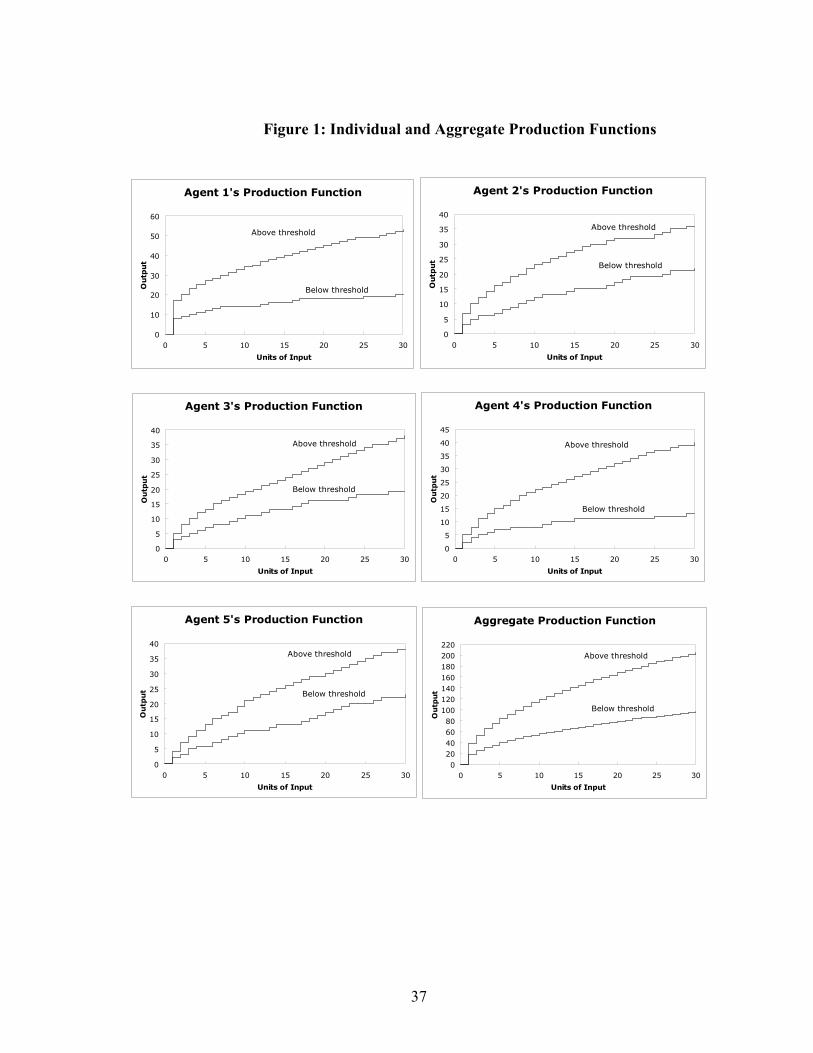
Figure 1: Individual and Aggregate Production Functions

Agent 1's Production Function

0

10

20

30

40

50

60

0 5 10 15 20 25 30

Units of Input

Outp

ut

Below threshold

Above threshold

Agent 2's Production Function

0

5

10

15

20

25

30

35

40

0 5 10 15 20 25 30

Units of Input

Outp

ut

Above threshold

Below threshold

Agent 3's Production Function

0

5

10

15

20

25

30

35

40

0 5 10 15 20 25 30

Units of Input

Ou

tpu

t

Above threshold

Below threshold

Agent 4's Production Function

0

5

10

15

20

25

30

35

40

45

0 5 10 15 20 25 30

Units of Input

Ou

tput

Above threshold

Below threshold

Agent 5's Production Function

0

5

10

15

20

25

30

35

40

0 5 10 15 20 25 30

Units of Input

Ou

tpu

t

Above threshold

Below threshold

Aggregate Production Function

020406080

100120140160180200220

0 5 10 15 20 25 30

Units of Input

Ou

tput

Above threshold

Below threshold

37

Figure 2: Individual and Aggregate Demand Functions

Agent 1's Demand Function

0

50

100

150

200

250

300

350

400

0 5 10 15 20 25

Units of K

Va

lue

Agent 2's Demand Function

0

50

100

150

200

250

300

350

400

450

0 5 10 15 20 25

Units of K

Valu

e

Agent 3's Demand Function

0

50

100

150

200

250

300

350

400

450

0 5 10 15 20 25

Units of K

Va

lue

Agent 4's Demand Function

0

50

100

150

200

250

300

350

400

450

0 5 10 15 20 25

Units of K

Valu

e

Agent 5's Demand Function

0

50

100

150

200

250

300

350

400

450

0 5 10 15 20 25

Units of K

Va

lue

Aggregate Demand Function

0

200

400

600

800

1000

1200

1400

1600

1800

2000

0 5 10 15 20 25

Units of K

Valu

e

38

Figures 3a-3d: Timing within a period

Baseline

Period t begins

Stage 1 Trading in call market

Stage 2 Allocation of output to ct

Determine if horizon ends

Period t ends Period t+1 begins

Transfer kt+1 into output (ct+1+kt+2)

Transfer kt into output (ct+kt+1) Voting

Period t begins

Stage 1 Trading in call market

Stage 2

Propose allocation of output to ct

Determine if horizon ends

Period t ends Period t+1 begins

Transfer kt+1 into output (ct+1+kt+2)

Transfer kt into output (ct+kt+1)

Vote for a proposed allocation

Period t begins

Stage 1 Trading in call market

S

Propoallocaof outct Transfer kt into

output (ct+kt+1)

Chat is allowed

Period t begins

Stage 1 Trading in call market

Transfer kt into output (ct+kt+1)

Chat is allowed

Communication

39

tage 2

se tion put to

Determine if horizon ends

Period t ends Period t+1 begins

Transfer kt+1 into output (ct+1+kt+2)

Chat is allowed

Vote for a proposed allocation

Stage 2 Allocation of output to ct

Determine if horizon ends

Period t ends Period t+1 begins

Transfer kt+1 into output (ct+1+kt+2)

Chat is allowed

Hybrid

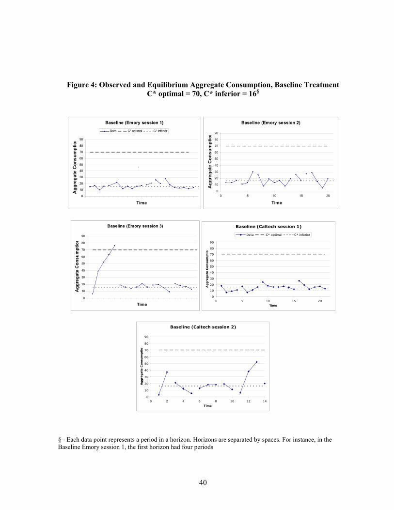
Figure 4: Observed and Equilibrium Aggregate Consumption, Baseline Treatment

C* optimal = 70, C* inferior = 16§

Baseline (Emory session 1)

0

10

20

30

40

50

60

70

80

90

Time

Agg

rega

te C

onsu

mpt

ion

Data C* optimal C* inferior

'

Baseline (Emory session 2)

0

10

20

30

40

50

60

70

80

90

0 5 10 15 20

TimeA

ggre

gate

Con

sum

ptio

n

Baseline (Emory session 3)

0

10

20

30

40

50

60

70

80

90

Time

Agg

rega

te C

onsu

mpt

ion

Baseline (Caltech session 1)

0

10

20

30

40

50

60

70

80

90

0 5 10 15 20

Time

Aggre

gate

Con

sum

pti

o

Data C* optimal C* inferior

Baseline (Caltech session 2)

0

10

20

30

40

50

60

70

80

90

0 2 4 6 8 10 12 1

Time

Aggre

gate

Con

sum

pti

o

4

§= Each data point represents a period in a horizon. Horizons are separated by spaces. For instance, in the Baseline Emory session 1, the first horizon had four periods

40

Figure 5: Observed and Equilibrium Aggregate Consumption, Communication Treatment; C* optimal = 70, C* inferior = 16

Communication (Emory session 1)

0

10

20

30

40

50

60

70

80

90

Time

Aggr

egat

e co

nsum

ptio

n

Data C* optimal C* inferior

Communication (Emory session 2)

0

10

20

30

40

50

60

70

80

90

Time

Agg

rega

te c

onsu

mpt

ion

Communication (Emory session 3)

0

10

20

30

40

50

60

70

80

90

Time

Aggr

egat

e co

nsum

ptio

n

Communication (Caltech session 1)

0

10

20

30

40

50

60

70

80

90

0 2 4 6 8 10 12 1

Time

Ag

gre

gate

Co

nsu

mp

tio

4

n

Data C* optimal C* inferior

Communication (Caltech session 2)

0

10

20

30

40

50

60

70

80

90

0 5 10 15

Time

Ag

gre

gate

Co

nsu

mp

tio

n

Communication (Caltech session 3)

0

10

20

30

40

50

60

70

80

90

0 5 10 15 20

Time

Ag

gre

gate

Co

nsu

mp

tio

n

41

Figure 6: Observed and Equilibrium Aggregate Consumption, Voting Treatment C* optimal = 70, C* inferior = 16

Voting (Emory session 1)

0

10

20

30

40

50

60

70

80

90

Time

Agg

rega

te C

onsu

mpt

ion

Data C* optimal C* inferior

Voting (Emory session 2)

0

10

20

30

40

50

60

70

80

90

Time

Agg

rega

te C

onsu

mpt

ion

Voting (Emory session 3)

0

10

20

30

40

50

60

70

80

90

Time

Agg

rega

te C

onsu

mpt

ion

Voting (Caltech session 1)

0

10

20

30

40

50

60

70

80

90

0 5 10 15 20

Time

Aggre

gate

Con

sum

pti

o

Data C* optimal C* inferior

Voting (Caltech session 2)

0

10

20

30

40

50

60

70

80

90

0 5 10 15 20

Time

Ag

gre

ga

te C

on

su

mp

tio

n

42

Figure 7: Observed and Equilibrium Aggregate Consumption, Hybrid Treatment; C* optimal = 70, C* inferior = 16

Hybrid (Emory session 1)

0

10

20

30

40

50

60

70

80

90

Time

Aggr

egat

e co

nsum

ptio

n

Data C* optimal C* inferior

Hybrid (Emory session 2)

0

10

20

30

40

50

60

70

80

90

Time

Agg

rega

te c

onsu

mpt

ion

Hybrid (Emory session 3)

0

10

20

30

40

50

60

70

80

90

Time

Agg

rega

te c

onsu

mpt

ion

Hybrid (Caltech session 1)

0

10

20

30

40

50

60

70

80

90

Time

Aggr

egat

e Co

nsum

ptio

n

Data C* optimal C* inferior

Hybrid (Caltech session 2)

0

10

20

30

40

50

60

70

80

90

Time

Aggr

egat

e Co

nsum

ptio

n

43

Figure 8: Observed and Equilibrium Prices, Baseline Treatment P* optimal = 118, P* inferior = 334

Baseline (Emory session 1)

0100200300400500600700800900

1000

Time

Pric

e of

K

P* optimal P* inferior Data

Baseline (Emory session 2)

0100200300400500600700800900

1000

Time

Pric

e of

K

Baseline (Emory session 3)

0100200300400500600700800900

1000

Time

Pric

e of

K

Baseline (Caltech session 1)

0100200300400500600700800900

1000

Time

Pric

e of

K

P* optimal P* inferior Data

Baseline (Caltech session 2)

0

100

200

300

400

500

600

700

800

900

1000

Time

Pric

e of

K

44

Figure 9: Observed and Equilibrium Prices, Voting Treatment P* optimal = 118, P* inferior = 334

Voting (Emory session 1)

0100200300400500600700800900

1000

Time

Pric

e of

K

P* inferior P* optimal Data

Voting (Emory session 2)

0100200300400500600700800900

1000

Time

Pric

e of

K

Voting (Emory session 3)

0100200300400500600700800900

1000

Time

Pric

e of

K

Voting (Caltech session 1)

0100200300400500600700800900

1000

Time

Pric

e of

K

P* inferior P* optimal Data

Voting (Caltech session 2)

0100200300400500600700800900

1000

Time

Pric

e of

K

45

Figure 10: Observed and Equilibrium Prices, Communication Treatment P* optimal = 118, P* inferior = 334

Communication (Emory session 1)

0100200300400500600700800900

1000

Time

Pric

e of

K

P* optimal P* inferior Data

Communication (Emory session 2)

0100200300400500600700800900

1000

Time

Pric

e of

K

Communication (Emory session 3)

0100200300400500600700800900

1000

Time

Pric

e of

K

Communication (Caltech session 1)

0100200300400500600700800900

1000

Time

Pric

e of

K

P* optimal P* inferior Data

Communication (Caltech session 2)

0100200300400500600700800900

1000

Time

Pric

e of

K

Communication (Caltech session 3)

0100200300400500600700800900

1000

Time

Pric

e of

K

46

Figure 11: Observed and Equilibrium Prices, Hybrid Treatment P* optimal = 118, P* inferior = 334

Hybrid (Emory session 1)

0100200300400500600700800900

1000

Time

Pric

e of

K

P* inferior P* optimal Data

Hybrid (Emory session 2)

0100200300400500600700800900

1000

Time

Pric

e of

K

Hybrid (Emory session 3)

0100200300400500600700800900

1000

Time

Pric

e of

K

Hybrid (Caltech session 1)

0100200300400500600700800900

1000

Time

Pric

e of

K

P* inferior P* optimal Data

Hybrid (Caltech session 2)

0100200300400500600700800900

1000

Time

Pric

e of

K

47

Figure 12: The relationship between inequality and welfare

Inequality and Welfare - Baseline

0

1

2

3

4

5

6

7

8

9

10

0 5000 10000 15000 20000

welfare level

coeff

icie

nt

of

vari

ati

on

Inequality and Welfare

0

1

2

3

4

5

6

7

8

9

10

0 5000 10000 15000 20000

welfare level

coeff

icie

nt

of

vari

ati

on

Inequality and Welfare - Voting

0

1

2

3

4

5

6

7

8

9

10

0 5000 10000 15000 20000

welfare level

coeff

icie

nt

of

vari

ati

on

Inequality and Welfare -Hybrid

0

1

2

3

4

5

6

7

8

9

10

0 5000 10000 15000 20000

welfare level

coeff

icie

nt

of

vari

ati

on

48

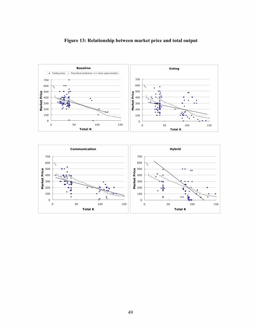
Figure 13: Relationship between market price and total output

Baseline

0

100

200

300

400

500

600

700

0 50 100 150

Total K

Mark

et

Pri

ce

Trading prices Theoretical predictions Linear approximation

Voting

0

100

200

300

400

500

600

700

0 50 100 150

Total KM

ark

et

Pri

ce

Communication

0

100

200

300

400

500

600

700

0 50 100

Total K

Mark

et

Pri

ce

150

Hybrid

0

100

200

300

400

500

600

700

0 50 100

Total K

Mark

et

Pri

ce

150

49

Figure 14a: Capital Stock and Number of Agents Communicating a Willingness to

Coordinate Investment, Communication Treatment

Communication (Emory session 1)

0

20

40

60

80

100

Time

K s

tock

K stock Threshold

03

00 3 4 1

2

5

2

10

01

Communication (Emory session 2)

0

20

40

60

80

100

Time

K s

tock

12 1 0 0 0 0 0

1

3

3 0

2

0

0

00

32

Communication (Emory session 3)

0

20

40

60

80

100

Time

K s

tock

0 00 0 0

0 00 0 1

0 00 0 0 0 0

0 10

Communication (Caltech session 1)

0

20

40

60

80

100

Time

K s

tock

K stock Threshold

2 23

42 0

12

0

0 30 3

0

Communication (Caltech session 2)

0

20

40

60

80

100

Time

K s

tock

0

4 5

44

3

5

0 00

0

0

00

0 0 0

Communication (Caltech session 3)

0

20

40

60

80

100

Time

K s

tock

5 0

0

30 0

00

0 0 0 0

4 0

00 0 0

0

0

50

Figure 14b: Capital Stock and Number of Agents Communicating A Willingness to

Coordinate Investment, Hybrid Treatment

Hybrid (Emory session 1)

0

20

40

60

80

Time

K s

tock

K stock Threshold

0

1

0

1

1

0

0

00

0

Hybrid (Emory session 2)

0

20

40

60

80

100

Time

K s

tock

0 1

0 10

0 0

0

0

0

0

00

0

Hybrid (Emory session 3)

0

20

40

60

80

100

Time

K s

tock

2

0

0

0

0 1

30 1

0

0 0

00

0

2

1

1

0

Hybrid (Caltech session 1)

0

20

40

60

80

100

Time

K s

tock

K stock Threshold

5 55 5

5

5 4 00 5 5 5 5

55

45

40

Hybrid (Caltech session 2)

0

20

40

60

80

100

Time

K s

tock

0 0 0 2 11

22

1 0

0 0

1

51

INSTRUCTIONS FOR EXPERIMENT

1. General Instructions This is an experiment in the economics of decision-making. The instructions are simple and if you follow them carefully and make good decisions, you might earn a considerable amount of money, which will be paid to you in cash at the end of the experiment. The amount of payment you receive depends partly on your decisions, partly on the decisions of others, and partly on chance. The currency used in the market is Yen. All trading will be in terms of the Yen. The cash payment to you at the end of the experiment will be in US dollars. The conversion rate is _____ Yen to 1 US dollar. Once the experiment has started, no one is allowed to talk to anybody other than the experimenter. Anyone who violates this rule will lose his or her right to participate in this experiment. In addition to your earnings from the activity in the experiment, you will receive a …… payment for your participation. 2. Basic Concepts The experiment will consist of a sequence of periods. At the beginning of each period, you will begin with a Cash Endowment of ______ Yen. You will also be given _____ units of a good called K on a one-time basis at the beginning of the first period of the experiment. In each period, there will be an open market. You will use this market to buy and sell units of K. Buying units of K reduces your cash by the amount of Yen that you pay for your purchases, whereas selling increases the cash you have by the amount that you receive for your sales. Thus, selling and buying K determines in part the earnings you make in each period. In addition, you will have a chance to choose how many units of K to consume. How much of K you consume during a period will also in part determine your earnings for the period. The K you do not consume can grow and can be sold or consumed in future periods. Your earnings in a period are equal to the amount of cash you have after buying and/or selling K minus the cash you began the period with, plus the earnings you receive from the consumption of K. A detailed explanation of how to buy, sell and consume units of K is given in section 3. Each period is divided into stages. In stage 1, you can buy and sell units of K. In stage 2, you decide how much to consume. In stage 3, the K you have is converted to a different quantity of K that you begin the next period with.

52

3. Stage 1: Buying and Selling Units of K The picture shown below is a copy of the first screen that you will see during Stage 1 of each period of the experiment. At the top of the screen you can find the Period number, the Total Earnings you have in Yen and the Remaining Time in seconds that you have to complete Stage 1. Below this information, you will find the number of Units of K You Hold, indicating the number of K that you currently have. You will also find the Units of K in the Economy, which is the total K that all five players currently have. You will also see the Cash Endowment for the period, indicating how much cash you currently have available for transactions.

3.1 Sending in Limit Prices to the Market You will use this screen to indicate the number of units of K you want to trade. You do so using the spaces Units of K and Limit Price. Under Units of K, you must enter a series of numbers in an increasing manner. The numbers will appear in the large window on the left portion of the screen. Type in a 1 for the first row, a 2 for the second row, a 3 for third row, etc… Enter as many numbers as the most units of K that you are willing to hold. The minimum quantity of units you can list is equal to the number of K you currently hold, the maximum quantity of units you can list is equal to the number of units in the economy. In the Limit Price field you must enter a limit price for each unit you list. The role of limit prices will be explained shortly. Each unit number must be accompanied by a limit price for the unit. The limit price will also appear in the large window on the left portion of the screen. Enter the limit price next to its corresponding unit. For example, if you enter 500 next to unit 1, it means that your limit price for the first unit is 500. If you enter a limit price of 450 next to the 2nd unit, it means that your limit price for the second unit is 450, and so on. The limit price for each additional unit must be less or equal to the previous one. For example, if you list a limit price of 123 Yen for the first unit, the second unit’s limit price must be equal or less than 123 Yen; similarly, the third unit’s price must be less or equal to the second unit’s price. All prices must be greater than zero. After entering units and limit prices, you must click on Update; you will see your choices recorded in the column entitled List of your choices. At any time you can modify your choice. You can also select the keys Erase all choices, which clears all of your limit prices, Erase last choice, which will remove the limit price for the highest-numbered unit, and Repeat, which will enter an identical limit price for the next unit. Once you are satisfied with your decision, you can send you limit prices to the market by clicking on Validate.

53

3.2 Finding how much you buy or sell Whether you will buy or sell units and how much you buy or sell depends on how your limit price compares to others’ limit prices, and how many units are in the economy. After all players have entered all of their limit prices and validated them, the prices that all players have sent in are ranked together from the highest to the lowest. Those who enter the highest prices will possess the units in the economy after stage 1. For example, suppose that there are ten units in the economy. Those that send in the ten highest limit prices will then receive the ten units in the economy. Often, the people who send in the highest limit prices will not be those who currently have the units. In that case, the people with the highest limit prices automatically purchase them from the people who currently have the units. Consider the following example. There are five players. Players 1, 2, and 3 each currently have one unit of K and players 4 and 5 do not have any units of K. Thus there are three units of K in the economy. Suppose that player 1 sends in a limit price of 500 for one unit of K. Player 2 sends in a limit price of 400 for one unit. Player 3 sends in a limit price of 600 for her first unit and 550 for her second unit. Player 4 sends in a bid of 630 for one unit. Player 5 sends in a limit price of 400 for one unit. In this example, player 3 receives two units and player 4 receives one unit of the total of three units

54

of K that exist in the economy. This means that players 1 and 2 each sell one unit (they each had one before and will not have any after the market process) and players 3 and 4 each purchase one unit (player 3 had one already before the market process and player 4 did not have any). As is clear from the above example, you are more likely to buy units for which the limit price is high and you are more likely to sell units for which the limit price is low compared to others’ limit prices. Of course, at the time you choose your prices, you will not know what other players are doing. You must send in a number of limit prices that is at least as great as the number of units of K you currently have. To purchase units, you must send in more than that number.

3.3 The price paid for purchases and sales When you are required to sell a unit you receive some cash from the sale, increasing your earnings. Likewise, when you purchase units you are required to spend cash to obtain the units, decreasing your earnings. The price at which participants buy and sell their units, which we will refer to as the market price, is determined in the following manner. When the limit prices are ranked from highest to lowest, we take the limit price that is ranked in the spot corresponding to the number of units of K in the economy. This price is called the market price. For example, for the limit prices described in the last subsection and three units in the economy, the third highest limit price submitted overall, the 550 player 3 sent in, becomes the market price. The market price is a per-unit price, so that if for example an individual buys five units, she pays five times the market price. 4. Consuming Units of K In each period, after stage 1 is completed, all players enter stage 2. Below you will find a picture of the screen you see in Stage 2. At the top of the screen you will see the current Period, your Total Earnings in Yen for the experiment so far and the Remaining Time you have to complete this stage in seconds. The data from Stage 1 and the results from trading are also on this screen. On your screen, you will see Units of K at Starting, which indicates the number of units you started the period with, the Units of K in the Economy, and your Cash Endowment. The screen also displays the Market Price, the price at which people bought and sold units in stage 1, K bought/sold on your part in stage 1, Cash transferred by you in stage 1 and Cash after trading, indicating how much cash you currently have.

55

Below these columns, you will see a row called Your Limit Prices summarizing the prices that you listed in Stage 1 for each unit; starting with the first unit and followed by the second, etc. A star separates these prices. The second row shows All Players’ Limit Prices. These are the prices that everyone in the market listed in Stage 1 for each of their units. The numbers are read in the following way. The parentheses indicate (the rank of the limit price, the limit price entered, the player who submitted the limit price). They are displayed in order from the highest limit price to the lowest. In this Stage, it will be decided how many of the units of K you currently have that you consume. Consuming a unit increases your earnings but removes the K you consume from your inventory and from the economy. How consumption affects your earnings in Yen for the period can be determined using your Redemption Value Sheet, which you received at the beginning of the experiment. 4.1 Redemption Value Sheet and Consumption The Redemption Value Sheet attached to these instructions shows the value in Yen from consuming units of K. The first column labeled Units of K consumed numbers the units from 1 through 28. The column labeled Unit Value indicates the additional amount of Yen you receive from consuming the unit indicated in the same row in the first column. The column

56

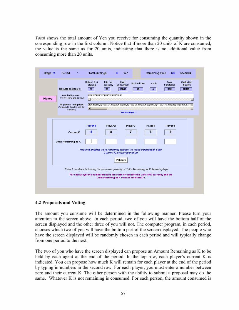
Total shows the total amount of Yen you receive for consuming the quantity shown in the corresponding row in the first column. Notice that if more than 20 units of K are consumed, the value is the same as for 20 units, indicating that there is no additional value from consuming more than 20 units.

4.2 Proposals and Voting The amount you consume will be determined in the following manner. Please turn your attention to the screen above. In each period, two of you will have the bottom half of the screen displayed and the other three of you will not. The computer program, in each period, chooses which two of you will have the bottom part of the screen displayed. The people who have the screen displayed will be randomly chosen in each period and will typically change from one period to the next. The two of you who have the screen displayed can propose an Amount Remaining as K to be held by each agent at the end of the period. In the top row, each player’s current K is indicated. You can propose how much K will remain for each player at the end of the period by typing in numbers in the second row. For each player, you must enter a number between zero and their current K. The other person with the ability to submit a proposal may do the same. Whatever K is not remaining is consumed. For each person, the amount consumed is

57

the difference between the Current K and the Units Remaining as K. For example, if player 1’s current K is 7 units, and he has 3 units remaining, he consumes 4 units. Select the validate button to submit the proposal to a vote. All five players will then see the following screen. The bottom half of the screen will display the two proposals. You can then vote for one of the proposals by the selecting the dark blue button on the right in the row corresponding to the proposal and selecting validate. The proposal that has a majority, three or more people, voting for it, is enacted. The program then indicates the final results for the period. Your consumption is indicated on the screen, as are your earnings from consumption (labeled earnings from units converted to C), which are calculated according to your Redemption Value Sheet.

5. Production The remaining K, that is, the amount of K that remains after you make your consumption decision, can be carried over to the next period. This K will be automatically converted to possibly more K. The amount that it is converted into is based on your Production Schedule. Thus, the amount of K you will have at the beginning of next period depends on

58

the remaining K you have after consuming at the end of the current period and on your Production Schedule. 5.1 Production Schedule The Production Schedule consists of two parts. When the total amount of K that the whole group has at the end of each period is less than or equal to 30, that is when the K in the Economy (that is the total Remaining K for all five people) is less than or equal to 30, use the left-hand-side of the Production Schedule to determine the amount of K that will be available to you at the beginning of next period. When the total remaining K in the economy exceeds 30, then you should use the right-hand-side of the schedule. In determining which side of the schedule is used, the total Remaining K is measured after consumption and before it grows at the beginning of the next period. Under the column labeled Remaining K you will find the number of units of K you have remaining after your consumption decision. The number next to it in the column labeled K at Market Open Next Period is the amount of good K that will available to you at the beginning of next period. The calculation for determining how many units of K you have in the next period is done automatically by the computer. 6. Summary of Period Earnings At the end of each period, the screen you see, entitled Final Results for Period will display a summary of the activity in the period. It will indicate your earnings in Yen for the period and your total earnings in the experiment thus far. Remember that earnings for the period in Yen are given by the cash endowment remaining after trading, minus your cash endowment at the beginning of the period, plus your earnings from consumption.

Earnings for a period in Yen = cash endowment remaining after trading – cash endowment at the beginning of the period + period earnings from consumption

7. Ending the Experiment The period in which the experiment ends is determined in the following way. Before the experiment began, the experimenter rolled a 10-sided die a series of times to determine how long the experiment would continue. If the die came up with number 1 or 2 on the first roll, then the game will end after the first period and there are no more die rolls. Otherwise, if the die roll resulted in a number from 3 to 10, the experiment will go on to the next period, and the die is rolled again. If the die came up 1 or 2 on the second roll, the experiment will end after period 2. In other words, in any given period, there is a fixed 20 percent chance (the odds are 2 in 10) that the experiment ends right after the current period. There is always a 80 percent chance that there will be at least one more period after the current one.

59

60

However, the experiment will be restarted if it ends with more than half an hour remaining during the time for which you have been recruited. If it is restarted, you will again begin with the same number of units that you started with in period 1. On the other hand, if the experiment is still in progress at the end of the time for which you have been recruited, the experiment will be continued on another afternoon or evening. The experimenter will run another session, in which the beginning holding of K for each individual will be the same as the end of the current session. You are free to participate in the continuation of the session with the same ID number, picking up from where you left off today. If you choose not to continue on with the session at a later date, another participant will be recruited to take your place. The earnings of the participant filling your place will also be given to you for the remainder of the life of the current series of periods. 8. The History Screen During stage 1 or stage 2, you can click on the button labeled History and you can access a history of your choices and of market activity for each past period. The information you can access includes the amount of K you held, the amount of K in the economy, your limit prices, the market price, the amount of K traded, the cash you have after trading, your earnings from consumption, the K remaining after your consumption, your period earnings, and your cumulative earnings 9. Communication with Other Subjects Before stage one, you will have an opportunity to communicate with other participants. You will see a screen in which there will be a field entitled Your Message. You are free to type in any messages you would like concerning the experiment, and all other subjects will be able to read them on their screens. They can also type in messages that you will be able to read.