the impact of oil price on south african gdp growth: a ... of pretoria department of economics...

University of Pretoria

Department of Economics Working Paper Series

The Impact of Oil Price on South African GDP Growth: A Bayesian Markov

Switching-VAR Analysis Mehmet Balcilar Eastern Mediterranean University, University of Pretoria

Reneé van Eyden University of Pretoria

Josine Uwilingiye University of Pretoria

Rangan Gupta University of Pretoria

Working Paper: 2014-70

November 2014

__________________________________________________________

Department of Economics

University of Pretoria

0002, Pretoria

South Africa

Tel: +27 12 420 2413

1

The impact of oil price on South African GDP growth: A Bayesian Markov Switching-

VAR analysis

Mehmet Balcilar*, Reneé van Eyden**, Josine Uwilingiye*** and Rangan Gupta****

Abstract

One characteristic of many macroeconomic and financial time series is their asymmetric

behaviour during different phases of a business cycle. Oil price shocks have been amongst those

economic variables that have been identified in theoretical and empirical literature to predict the

phases of business cycles. However, the role of oil price shocks to determine business cycle

fluctuations has received less attention in emerging and developing economies. The aim of this

study is to investigate the role of oil price shocks in predicting the phases of the South African

business cycle associated with higher and lower growth regimes. By adopting a regime dependent

analysis, we investigate the impact of oil price shocks under two phases of the business cycle,

namely high and low growth regimes. As a net importer of oil, South Africa is expected to be

vulnerable to oil price shocks irrespective of the phase of the business cycle. Using a Bayesian

Markov switching vector autoregressive (MS-VAR) model and data for the period 1960Q2 to

2013Q3, we found the oil price to have predictive content for real output growth under the low

growth regime. The results also show the low growth state to be shorter-lived compared to the

higher growth state.

Keywords: Macroeconomic fluctuations, oil price shocks, Bayesian Markov switching

VAR

JEL Codes: C32, E32, Q43

* Department of Economics, Eastern Mediterranean University, Famagusta, Northern Cyprus , via Mersin 10, Turkey; Department of Economics, University of Pretoria, Pretoria, 0002, South Africa. Email: [email protected]. ** Corresponding author. Department of Economics, University of Pretoria, Pretoria, 0002, South Africa. Email: [email protected]. *** Department of Economics and Econometrics, University of Johannesburg, Auckland Park, 2006, South Africa. Email: [email protected]. **** Department of Economics, University of Pretoria, Pretoria, 0002, South Africa. Email: rangan.gupta @up.ac.za.

2

1. Introduction

The role of oil price shocks on macroeconomics variables emerged after the 1973 and 1979 oil

price shocks that coincided with a period of high inflation, high unemployment and decelerating

economic activities in a number of countries. Since then, macroeconomists have focused their

attention on the macroeconomic consequences of oil price shocks. In economics, a number of

transmission channels exist through which oil price affects output. From the supply side, an

increase in the oil price will lead to higher input costs which will increase the cost of production

of goods and services. The production volume may thus be affected, as firms may find it difficult

in the short run to re-allocate resources in order to produce the same volume of goods and

services. The magnitude of the impact of oil price shocks to the aggregate output will however

depend on the energy intensity in the production process. On the demand side, an increase in

the oil price will put pressure on the price level. In order to control the inflation, the central bank

might increase the interest rate, which could lead to a reduction in investment, and hence a

decline in output. Moreover, the increase in oil price affects the individual consumer as it will

reduce the amount of goods and services that could be purchased with the consumer’s existing

level of income.

A number of studies have been conducted to investigate the linear relationship between

oil price shocks and economic activities; using Sims’ (1980) linear VAR model with the aid of

impulse response analysis. In most instances, research findings reveal the existence of a negative

relationship between oil prices shocks and economic activities; however the strength of the

relationship in different countries are likely to depend on the energy intensity, structure of the

economy and the sample period (Abeysinghe 2001; Nkomo 2006; and Tang, et al. 2010). Despite

the evidence of an overall negative relationship between oil price and economic activity observed

in a number of studies, when the oil price decreased significantly, by as much as 50 per cent in

real terms, during the first half of 1986, for a number of countries it was found that the decline

in oil price did not promote economic growth, giving rise to a renewed debate on oil price

effects on economic activity. A number of studies consequently focused on the possibility of a

nonlinear and asymmetric relationship between oil price and economic activity.

Mork (1989) in his study on the role of oil price shocks on economic activity, finds oil

price increases to affect economic growth negatively while a decline in oil price does not have

the opposite effect. Where the coefficients on oil price increases turn out to be negative and

highly significant, the coefficients on price declines tend to be positive, but small and not

statistically significant. Hamilton (1988) provides a theoretical framework to explain the source

3

of asymmetry in the relationship between oil price and real output. The author observes that

when the growth rate of oil price increases, durable consumption growth drops, as consumers

choose to postpone their purchases. But when the growth rate of the price of oil slows down,

durable consumption growth does not necessarily rise. Hooker (1996) reports an insignificant

relationship between oil price shocks and US macroeconomic variables in the period following

the 1973 oil price shock. Herrera, et al. (2011), investigate the presence of a linear relationship

between an oil price shock and economic activity. Using industrial production as a measure of

economic activity, the results fail to show any asymmetric relationship between oil price and

industrial production at the aggregated level. Using data on industrial production at a

disaggregated level however, the authors find strong evidence of a nonlinear and asymmetric

relationship between oil price and output for industries that are energy intensive or produce

goods that are energy intensive in use. Blanchard and Gali (2007) find that despite similar energy

intensity levels for the four oil price shocks identified in their study, the effect of these shocks on

growth and inflation has been different for different shocks. The 1970s shocks were

characterised by higher inflation and lower growth while in the more recent period lower

inflation and increasing growth are observed despite the on-going increase in energy

consumption over time. The authors linked the recent dynamics of oil shocks on

macroeconomic variables to a better monetary policy, a decrease in wage rigidities and a

reduction of oil usage in production processes. Given the findings in a number of studies of a

weakened relationship between oil shocks and economic activity observed for recent periods,

and the fact that the effect of oil price increases seem to matter in a nonlinear setting, studies

that use linear models may be incapable to capture the dynamics between oil prices shocks and

economic activities accurately. Another interesting observation arises in the study by Kilian

(2009), where the author argues that the impact of oil shocks on macroeconomic variables

depends on the source of the oil shock. In his study, he considers oil supply shocks, global

demand shocks and oil demand shocks. One of the conclusions of his analysis is that emphasis

on oil supply shocks which is exogenous in explaining the impact of oil price shocks on

macroeconomic variables might be misleading. In South Africa, a recent study by Chisadza, et al.

(2013) investigates the impact of oil shocks on the South African economy using a sign

restriction-based structural vector autoregressive (VAR) model. Considering oil supply shocks,

oil demand shocks driven by global economic activity, and oil-specific demand shocks, the

authors found output to be affected positively by both oil demand and oil-specific demand

shocks, while oil supply shock has no significant effect on output. Aye et al., (2014) analyzes the

impact of oil price uncertainty on manufacturing production of South Africa using a bivariate

4

GARCH-in-mean-VAR model, and shows oil price uncertainty to have a significant negative

impact on manufacturing production. In addition, the paper also detects that the response of

manufacturing production to positive and negative shocks are asymmetric.

Oil price shocks have also been identified in a number of studies as one of the

contributing factors influencing the state of the business cycle. For the US economy, Hamilton

(1983, 1996 and 2005), finds that an increase in the oil price has preceded almost all the

recessions in the US, which finding has attracted a number of researchers to investigate the role

of an oil price shock in predicting business cycle fluctuations. Raymond and Rich (1997) use a

generalized Markov switching (MS) model, where net oil price increase is included in the model

to examine its contribution to post-war US business cycle fluctuations. The authors confirm the

oil price to be a contributing factor to phases of low output. However, the study finds oil prices

not to predict the transition from the low growth to high growth phases of the business cycle.

Moreover, the authors are of the opinion that the Hamilton (1983) study overstates the role of

oil price shocks in predicting a recession. De Miguel, et al. (2003), employ a standard dynamic

stochastic general equilibrium (DSGE) model for the small open Spanish economy, and include

the oil price shock in the model as an exogenous technological shock and as the only source of

fluctuation in economic activity. The study then analyses the effects of the shock on business

cycle fluctuations and on welfare. Their model results are in line with the business cycle path of

the Spanish economy; specifically, a negative impact of an increase in relative price of oil on

welfare was identified. Schmidt and Zimmermann (2005) find the effect of an oil shock on

German business cycle fluctuation to be limited and declining over time when the analysis is split

into sub-periods of 1970-1986 and 1997-2002. The limited effect of oil price changes on the

business cycle is also reported on in the study by Kim and Loungani (1992). Clements and

Krolzig (2002) use a three-state Markov switching VAR (MS-VAR) to test whether oil prices can

explain business cycle asymmetries. The authors find that oil prices movements cannot

adequately explain business cycle asymmetries. Using a Markov switching analysis for the G-7

countries, Cologni and Manera (2006) investigate the asymmetric effect of an oil shock on

different phases of the business cycle for each of the G-7 countries; and find regime dependent

models to better capture the output growth process. Recently, Engemann, et al. (2010), using a

Markov switching model, investigated whether oil price shocks significantly increase the

probability of a recession in a number of countries and found oil price to affect the likelihood of

moving into recession.

Despite significant evidence of the role of oil price shocks in explaining business cycle

movement for the US and other developed countries, a limited number of studies have been

5

conducted for developing countries to investigate the transmission of oil price shocks to

economic activity. The effect of oil price shocks on macroeconomic variables in the case of

developing economics also vary significantly across countries, due to the disparity in the degree

of energy intensity of the economy, the size of the shock and economic structure of the country.

South Africa as a net oil importer, consumes the second-largest amount of petroleum in Africa,

behind Liberia; and 95 per cent of its crude oil needs are met through imports. South Africa

imports crude oil mostly from OPEC countries in the Middle East and West Africa, with

roughly half of imported oil coming from Saudi Arabia in 2013. Given the importance of oil in

South African economy, the present paper investigates the impact of oil price shocks on South

African business cycle fluctuation using a two-state Bayesian Markov switching VAR, the

asymmetric response of oil shocks during high and low growth phases of the business cycle will

be analysed through state-dependent impulse responses.

The Markov switching model used in this study has been widely used in empirical literature

to capture nonlinearities and asymmetry among economic variables (Hamilton 1994; Krolzig

2001; and Krolzig and Clements 2002). First, the model allows us to classify regimes as

depending on the parameter switches in the full sample and, therefore, it is possible to detect

changes in dynamic interactions between the variables. Second, this model allows for many

possible changes in the dynamic interactions between the variables at unknown periods. Third, it

is possible to make probabilistic inference about the dates at which a change in regime occurred.

To date, no study to our knowledge has been undertaken to investigate the effect of oil price

shocks on South African business cycle fluctuations, using a MS-VAR model.1

The rest of the sections are outlined as follows: Section 2 discusses the methodology used

in this study, Section 3 presents data, section 4 discusses the empirical findings, and Section 5

concludes.

2. Methodology

It is commonly accepted that one of the most important challenges facing macroeconometric

time series models is structural change or regime shift (see Granger, 1996). Indeed, the survey

papers by Hansen (2001) or Perron (2006) affirm that econometric applications should distinctly

consider regime shifts.

Econometricians have recently introduced new models that can sufficiently deal with

1 However, there does exist recent studies that have analyzed the (symmetric and asymmetric) impact of oil price shocks on inflation (Ajmi et al., 2014; Gupta and Kanda, 2014) and interest rates (Aye et al., forthcoming) for South Africa, in both time and frequency domains.

6

certain types of structural changes. One of the appealing methodologies that can deal with

structural breaks is the Markov switching (MS) approach proposed by Hamilton (1990) and later

extended to multivariate time series models by Krolzig (1997). The initial work by Hamilton

(1990) studies univariate Markov switching autoregression (MS-AR) while a multivariate

extension to Markov switching vector autoregression (MS-VAR) is introduced in Krolzig (1997).

The MS models fall within the category of nonlinear time series models which is generated by

nonlinear dynamic properties, such as high moment structures, time varying, asymmetric cycles,

and jumps or breaks in a time series (Fan and Yao, 2003). The long time span of our data

includes several influential events, such as the first and second OPEC oil price shocks in 1973

and 1979, respectively, the debt-standstill agreement and economic sanctions imposed against

South Africa in 1985 as a consequence of its Apartheid regime, the relaxation of trade sanctions

again and the transition to a democracy in 1994, the 1997/98 East Asian crisis, and more

recently the global recession of 2008. The data also covers quite a number of influential business

cycles. MS models are found to fit well to such time series data with business cycles features and

regime shifts.

A number of studies successfully used MS models to analyse aggregate output and

business cycles (e.g., Hamilton 1989; Diebold, et al. 1994; Durland and McCurdy 1994; Filardo

1994, Ghysels 1994; Kim and Yoo 1995; Filardo and Gordon 1998; and Krolzig and Clements

2002). Following these studies, we thus consider the MS-VAR model, which, with its rich

structure, accommodates the features of oil price and output data we examine. The model choice

unlike other traditional models not only efficiently captures the dynamics of the process, but also

has a more appealing structural form and provides economically intuitive results.

The methodology we adopt is based on a vector autoregressive (VAR) model with time-

varying parameters where, given our objectives, the parameter time-variation directly reflects

regime switching. In this approach, changes in the regimes are treated as random events

governed by an exogenous Markov process, leading to the MS-VAR model. The state of the

economy is determined by a latent Markov process, with probability of the latent state process

taking a certain value based on the sample information. In this model, inferences about the

regimes can be made on the basis of the estimated probability, which is the probability of each

observation in the sample coming from a particular regime. The MS-VAR model we use to

analyse the time varying dynamic relationship between the quarterly real spot crude oil price and

real GDP is an extension of the class of autoregressive models studied in Hamilton (1990) and

Krishnamurthy and Rydén (1998). It also allows for asymmetric (regime dependent) inference

for impulse response analysis. The structure of the MS-VAR model we use is based on the

7

model studied in Krolzig (1997) and Krolzig and Clements (2002). Our estimation approach is

based on the Bayesian Markov-chain Monte Carlo (MCMC) integration method of Gibbs

sampling, which allows us to obtain confidence intervals for the impulse response functions of

the MS-VAR model.

To be concrete, let Pt and Qt

denote the real crude oil price and real output2, respectively.

Define the time-series vector up to and including period t as Xt = [Pt ,Qt ′] and let

, where p is a nonnegative integer. For

the vector valued time series of random variables, assume that a density (probability)

function exists for each t ∈ 1, 2,…,T. The parameters and the parameter space

are denoted by θ and Θ, respectively. The true value of θ is denoted by θ0 ∈ Θ. Let the stochastic

variable follow a Markov process (chain) with q states. In the MS-VAR model,

the latent state variable determines the probability of a given state in the economy at any

point in time. Taking into account that the oil price and output series are not cointegrated and

their dynamic interactions are likely to have time-varying parameters, our analysis is based on the

following MS-VAR model:

∆Xt= µ

St

+ ΓS

t

(k )

k=1

p−1

∑ ∆Xt−k

+ εt, t = 1,2,...,T

(1)

where p is the order of the MS-VAR model, [ | ~ (0, )]t t stS Nε Ω , and is a (2 × 2) positive

definite covariance matrix. The random state or regime variable , conditional on , is

unobserved, independent of past Xs, and assumed to follow a q-state Markov process. In other

words, Pr[St = j St−1 = i ,St−2 = k2,,ℑt−1] = Pr[St = j St−1 = i ,ℑt−1] = pij

, for all t and , regimes

i, j = 1, 2, ..., q, and l ≥ 2. More precisely follows a q state Markov process with transition

probability matrix given by

. (2)

Thus, pij is the probability of being in regime j at time t, given that the economy was in

regime i at time (t-1), where i and j take possible values in 1, 2,…, q. The MS-VAR specified as

above allows all parameters to depend on the latent regime or state variable St, that is all

2 The real crude oil price and real GDP series we analyse are both nonstationary time series as shown by the unit root tests reported on in Section 3. Moreover, the series also do not maintain a long-run relationship as they are not cointegrated, leading to a MS-VAR model in first differences.

Xt

ℑt = Xτ τ = t,t −1,...,1− p) ℑt = Xτ τ = t,t −1,...,1− p)

Xt

f (Xt ℑt−1,θ )

St ∈1,2,...,q

St

ΩSt

St St−1

kl

St

8

parameters of the model including the variance matrix .

In our particular application, the maintained hypothesis is that q=2, that is, two states or

regimes for each variable are sufficient to describe the dynamic interactions between the oil price

and output. This is consistent with crises-recovery (recession-expansion) cycles observed in

many macroeconomic time series. A large number of studies showed that the two regime MS

model is rich enough to capture the regime switching behaviour in macroeconomic time series

(e.g., Hamilton 1989; Diebold, et al. 1994; Durland and McCurdy 1994; Filardo 1994, Ghysels

1994; Kim and Yoo 1995; Filardo and Gordon 1998; and Krolzig and Clements 2002).

The MS-VAR model in Equations (1)-(2) has some appealing properties for analysing the

dynamic interactions of the variables. First, it allows us to classify regimes as depending on the

parameter switches in the full sample and, therefore, it is possible to detect changes in dynamic

interactions between the variables. Second, this model allows for many possible changes in the

dynamic interactions between the variables at unknown periods. Third, it is possible to make

probabilistic inference about the dates at which a change in regime occurred. We will be able to

evaluate the extent of whether a change in the regime has actually occurred, and also identify the

dates of the regime changes. Finally, this model also allows us to derive regime dependent

impulse response functions to summarize whether the impact of the oil price on the GDP varies

with regimes.

The empirical procedure for building a suitable MS-VAR models starts with identifying a

possible set of models to consider. We determine the order p of the MS-VAR model using the

Bayesian information Criterion (BIC) in a linear VAR(p) model. The MS-VAR model

specifications may differ in terms of regime numbers (q) and the variance matrix specification.

We only consider both regime-dependent (heteroscedastic) variance models, because both the oil

price and output series span a number of periods where volatilities vary significantly. Once a

specific MS-VAR model is identified, we next test for the presence of nonlinearities in the data.

When testing the MS-VAR model against the linear VAR alternative, we follow Ang and Bekaert

(2002) and use the likelihood-ratio statistic (LR), which is approximately χ2(q) distributed, where

q equals the number of restrictions plus the nuisance parameters (i.e., free transition

probabilities) that are not identified under the null. We use p-values based on the conventional χ2

distribution with q degrees of freedom and also for the approximate upper bound for the

significance level of the LR statistic as derived by Davies (1987). Once we establish nonlinearity,

we can choose the number of regimes and the type of the MS model based on both the

ΩSt

9

likelihood-ratio statistic and the Akaike information Criterion (AIC).3

There are three commonly used methods used for estimating the parameters of MS

models. Although the simplest method of estimation is maximum likelihood (ML), it may be

computationally demanding and may have slow convergence. 4 The ML method faces two

important practical difficulties. First, a global maximum of the likelihood may be difficult to

locate. Second, the likelihood function for the important class of mixtures of normal

distributions is not bounded and the ML estimator does not exist for the global maximum.

Second, and more commonly used, the method of estimation for MS models is the expectation

maximization (EM) algorithm (Dempster, et al. 1977; Lindgren 1978; Hamilton 1990, 1994).

Assuming that the conditional distribution of Xt given is normal, the

likelihood function is numerically approximated using the EM algorithm in two steps. In the first

step, given the current parameter estimates and the data, the conditional expectation of log

likelihood is computed (E-step), and in the second step parameters that maximize the complete-

data log likelihood function computed (M-step). The EM algorithm may have slow convergence

and also standard errors of the parameters cannot be directly obtained from the EM algorithm.

A third method is the Bayesian MCMC parameter estimation based on Gibbs sampling. The ML

and EM methods usually fail for certain types of models since it may not be possible to compute

the full vector of likelihoods for each regime for each period. The MCMC works only with one

sample path for the regimes rather than a weighted average of sample paths over all regimes, and

therefore, avoids the problem faced by the ML and EM methods.

The MCMC indeed treats the regimes as a distinct set of parameters. Our MCMC

implementation is based on the following steps5:

i. Draw the model parameters given the regimes. In our case, transition probabilities do

not enter this step.

ii. Draw the regimes given the transition probabilities and model parameters.

iii. Draw the transition probabilities given the regimes. In our case, model parameters do

not enter this step.

In the next step, we first draw ΩStgiven regimes, P, and ηSt

= (β,µSt,αSt

,ΓSt′) using a

hierarchical prior. Our implementation first draws a common covariance matrix from the

Wishart distribution given the inverse of the regime specific covariances; and second we draw

3 Krolzig (1997) and Psaradakis and Spagnolo (2003) suggest selecting the number of regimes and the MS model using the AIC, and using a Monte Carlo experiment Psaradakis and Spagnolo (2003) show that the AIC generally yields better results in selecting the correct model. 4 An excellent review of the ML estimation of the MS models is provided by Redner and Walker (1984). 5 See Fruehwirth-Schnatter (2006) for the details of the MCMC estimation of the MS models.

ℑ

t,S

t,S

t−1,...,S

0; ′θ

10

the regime specific covariances from the inverse Wishart distribution given the common

covariance. The degrees of freedom priors for Wishart and inverse Wishart distributions are

both equal to 4. Second, we use a flat prior and draw ηSt= (β,µSt

,αSt,ΓSt

′) given regimes, P,

and ΩSt from a multivariate Normal distribution with 0 mean. In the second step, we draw

regimes St given ηSt= (β,µSt

,αSt,ΓSt

′) , P, and ΩSt. This is obtained from the Bayes formula,

where the relative probability of regime i at time t is given as the product of the unconditional

regime probability times the likelihood of regime i at time t. Regimes are drawn as a random

index from 1,…,q given relative probability weights. Indeed, we use the Forward Filter-

Backwards Sampling (FFBS) (also called Multi Move Sampling) algorithm described in Chib

(1996) to draw the regimes. In the second step of the MCMC method we reject any draw, if less

than 5% of the observations fall in any of the regimes. Finally, in the third step, unconditional

probabilities P given the regimes are drawn from a Dirichlet distribution. We set the priors for

the Dirichlet distribution as 80% probability of staying in the same regime and 20% probability

of switching to the other regime. We perform the MCMC integration with 50,000 posterior

draws with a 20,000 burn-in draws.

Since its first introduction in the influential work of Sims (1980), a natural tool to analyse

the dynamic interaction between the oil price variable and output is the impulse response

function (IRF). IRF analysis studies how a given magnitude of a shock in one of the variables

propagates to all variables in the system over time, say for h=1,2,…, H steps after the shock hits

the system. Computing multi-step IRFs from MS-VAR models as well as from all nonlinear time

series models prove complicated because no ordinary method of computing the future path of

the regime process exists. An ideal IRF analysis requires that we know the future path of the

regime process, since the impulses depend on the regime of the system in every time period.

Ideally, the IRFs of the MS-VAR model should integrate the regime history into the

propagation period, which is not easily resolved. Two approaches arose in the literature as a

work-around to the history dependence of the IRS in the MS models. Ehrmann et al. (2003)

suggested assuming that regimes do not switch beyond the shock horizon, leading to regime-

dependent IRFs (RDIRFs). On the other hand, Krolzig (2006) acknowledges the history

dependence and allows the regime process to influence the propagation of the shocks for the

period of interest, h=1, 2, … H. In Krolzig’s approach conditional probabilities of future

regimes, St+h, are obtained given the regime St

and the transition probabilities, P.

One major attraction of the RDIRF analysis is the possibility of determining the time

variation in the responses of variables to a particular shock. The RDIRF traces the expected path

11

of the endogenous variable at time t+h after a shock of given size to the k-th initial disturbance at

time t, conditioned on regime i. The k-dimensional response vectors ψki,1,…, ψki,h represents a

prediction of the response of the endogenous variables. (Ehrmann, et al. 2003). The RDIRFs6

can be defined as follows:

ψ

ki,h=

∂Et Xt+h

∂uk,t St=⋅⋅⋅=S

t+h=i

for h ≥ 0 (3)

where uk ,t is the structural shock to the k-th variable. In general, the reduced form shocks ε

t

will be correlated across the equations and ε k ,t will not correspond to uk ,t

. This leads to the

famous identification problem for which several solutions exist. We assume that the structural

shocks are identified as ε t = FStut. To make structural inferences from the data, the structural

disturbances and hence F must be identified. In other words, sufficient restrictions are imposed

on the parameter estimates in order to derive a separate structural form for each regime, from

which RDIRFs are then computed. As in a standard VAR measuring the impact of the oil prices

on output, we order the output last and use the recursive identification scheme, made popular by

Sims (1980). The recursive identification scheme is based on the Cholesky decomposition of the

covariance matrix as ΩSt= LSt

′LSt and identifying structural shocks from ut = FSt

−1ε t with

FSt= LSt

.

The RDIRF analysis, although significantly simplifies derivation and allows construction of

confidence interval via bootstrap, it is not appropriate, if the regime switching is likely during

propagation of shocks. The solution of Krolzig (2006) is appealing, but it leaves out the

construction of the confidence intervals. In our study, we combine RDIRF analysis with MCMC

integration. Given our interest is whether the dynamic response of the output to oil price shocks

depends on the state of the economy, such as the recession or recovery periods, assuming a

given regime − regime switching does not take place during the shock propagation periods − and

studying the propagation of the oil price shock in the future is appropriate for our purpose.

Building on the Bayesian impulse responses for the linear VAR models, which are well covered

in Ni, et al. (2007), we drive the posterior density of the RDIRFs from the Gibbs sampling. The

simulations of the posteriors of the parameters jointly with the identification of the structural

shocks via the Gibbs sampler directly yield the posterior densities of the RDIRFs. The

confidence bands are obtained by the MCMC integration with Gibbs sampling of 50,000

posterior draws with a burn-in of 20,000.

6 Refer to Ehrmann, et al. (2003) for details on characteristics and computation of the regime-dependent impulse responses.

12

3. Data

In this study, we employ quarterly data for the period 1960Q1-2013Q3 for real GDP and real oil

price. We make use of real gross domestic product (GDP) at market prices from the South

African Reserve Bank, and to obtain quarterly real oil price in South African currency, we use the

nominal Brent crude oil spot price from the US Department of Energy as the main source

(DCOILBRENTEU, 1987Q3-2013Q4) but supplement it further back with data from Global

Financial Data (GFD) (BRT-D, 1970Q1-1987Q2). Since the spread between Brent crude and the

WTI oil price in early years of the sample appears very small, we use WTI's oil price data to

supplement for the 1960s. Nominal oil price data are seasonally adjusted using the X-12

procedure and converted into Rand values using the Rand/US$ exchange rate from GFD from

1960Q1-2012Q3. Lastly, nominal values are deflated using CPI from the International Financial

Statistics (IFS) of the International Monetary Fund (IMF) to obtain the real oil price. Figure 1

shows the time series of the real Brent crude oil price in South African Rand, and the real gross

domestic product. All values are expressed in natural logarithms. The sample period covers

1960Q1 – 2013Q3.

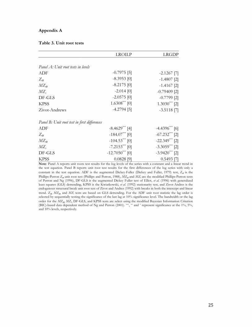
Different unit root tests were performed to investigate the univariate characteristics of

both level variables. The set of formal unit root tests presented in Appendix A reveals that both

variables are I(1), hence nonstationary in levels but stationary after first differencing. Given the

nonstationarity of the log of real GDP and log of real oil price, in order to estimate the MS-VAR

model, we make use of the growth of real GDP and growth of real oil price which are both

stationary or I(0). The sample period used to estimate the MS-VAR is 1960Q2 to 2013Q3.

4. Empirical findings

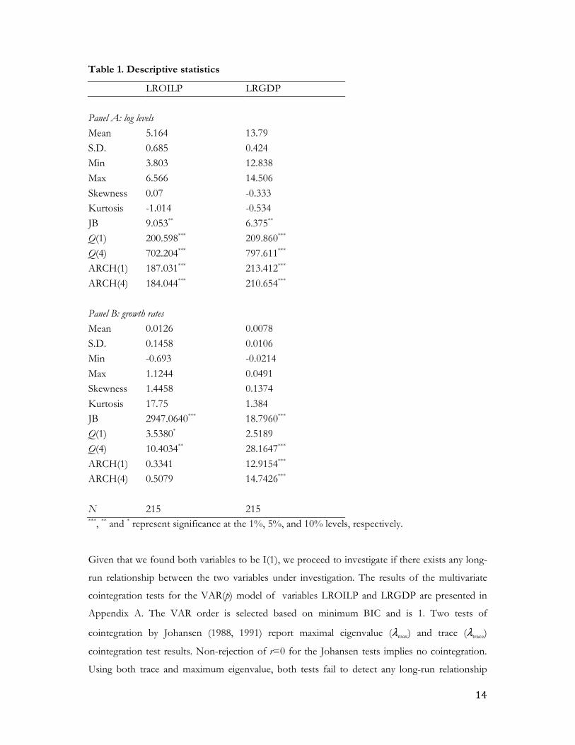
Before we start estimating our models, we first contemplate some preliminary descriptive

statistic on quarterly real Brent crude oil spot price in South African Rand (LROILP), and the

quarterly real GDP of South Africa (LRGDP). The graphic representations and summary

statistics on both variables are presented in Figure 1 and Table 1, respectively.

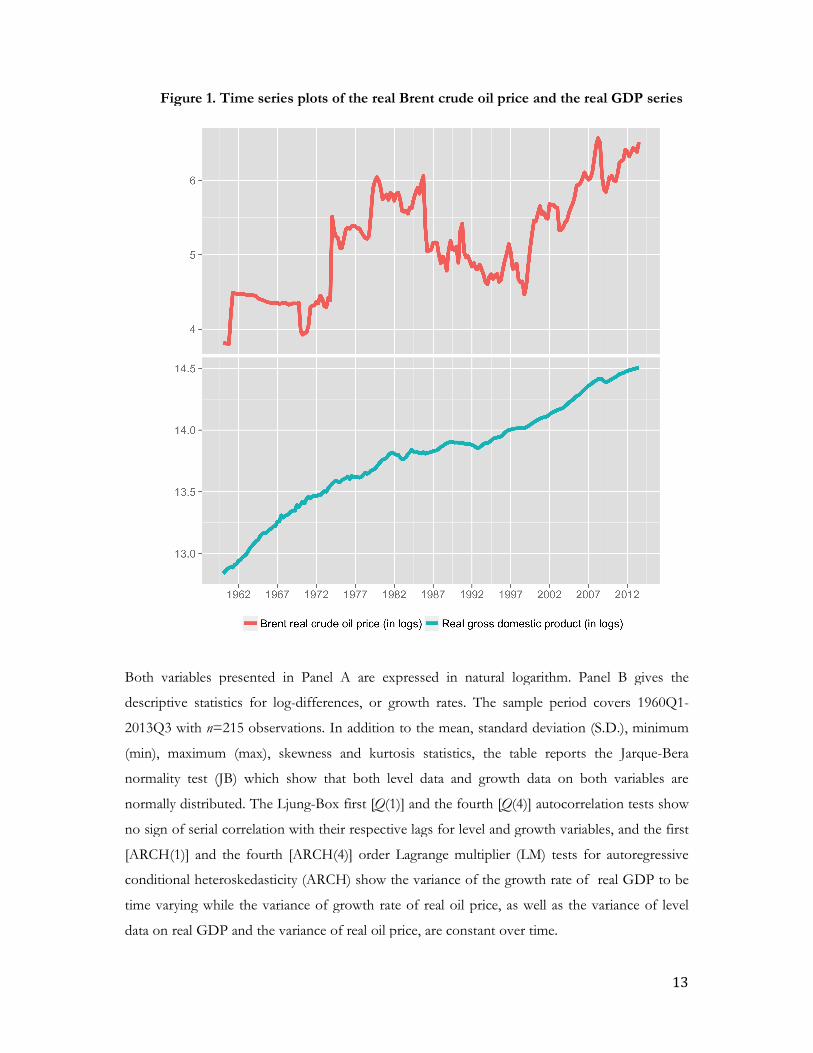
Figure 1. Time series plots of the real Brent crude oil price and the real GDP series

Both variables presented in Panel A are expressed in natural logarithm. Panel B gives the

descriptive statistics for log-differences, or growth rates. The sample period covers 1960Q1

2013Q3 with n=215 observations.

(min), maximum (max), skewness and kurtosis statistics, the table reports the Jarque

normality test (JB) which show that both level data and growth data on both variables are

normally distributed. The Ljung-Box first [

no sign of serial correlation with their respective lags for level and growth variables, and the first

[ARCH(1)] and the fourth [ARCH(4)] order Lagrange multiplier (LM) tests for autoregressive

conditional heteroskedasticity (ARCH) show the variance of the growth rate of real GDP to be

time varying while the variance of growth rate of real oil price, as well as the variance of level

data on real GDP and the variance of real oil price, are constant over time.



differences, or growth rates. The sample period covers 1960Q1

=215 observations. In addition to the mean, standard deviation (S.D.), minimum

(min), maximum (max), skewness and kurtosis statistics, the table reports the Jarque


Box first [Q(1)] and the fourth [Q(4)] autocorrelation tests show



edasticity (ARCH) show the variance of the growth rate of real GDP to be


data on real GDP and the variance of real oil price, are constant over time.

13



differences, or growth rates. The sample period covers 1960Q1-

ion (S.D.), minimum

(min), maximum (max), skewness and kurtosis statistics, the table reports the Jarque-Bera


(4)] autocorrelation tests show



edasticity (ARCH) show the variance of the growth rate of real GDP to be


14

Table 1. Descriptive statistics

LROILP LRGDP

Panel A: log levels

Mean 5.164 13.79

S.D. 0.685 0.424

Min 3.803 12.838

Max 6.566 14.506

Skewness 0.07 -0.333

Kurtosis -1.014 -0.534

JB 9.053** 6.375**

Q(1) 200.598*** 209.860***

Q(4) 702.204*** 797.611***

ARCH(1) 187.031*** 213.412***

ARCH(4) 184.044*** 210.654***

Panel B: growth rates

Mean 0.0126 0.0078

S.D. 0.1458 0.0106

Min -0.693 -0.0214

Max 1.1244 0.0491

Skewness 1.4458 0.1374

Kurtosis 17.75 1.384

JB 2947.0640*** 18.7960***

Q(1) 3.5380* 2.5189

Q(4) 10.4034** 28.1647***

ARCH(1) 0.3341 12.9154***

ARCH(4) 0.5079 14.7426***

N 215 215 ***, ** and * represent significance at the 1%, 5%, and 10% levels, respectively.

Given that we found both variables to be I(1), we proceed to investigate if there exists any long-

run relationship between the two variables under investigation. The results of the multivariate

cointegration tests for the VAR(p) model of variables LROILP and LRGDP are presented in

Appendix A. The VAR order is selected based on minimum BIC and is 1. Two tests of

cointegration by Johansen (1988, 1991) report maximal eigenvalue (λmax) and trace (λtrace)

cointegration test results. Non-rejection of r=0 for the Johansen tests implies no cointegration.

Using both trace and maximum eigenvalue, both tests fail to detect any long-run relationship

15

between the variables. Stock and Watson (1988) common trends testing confirms that the real oil

prices and real GDP series are not cointegrated. Since Johansen cointegration tests fail to show

any existence of a long-run relationship between real oil prices and real GDP, we then proceed

our estimation using a Bayesian MS-VAR with 4 lags form 1960Q2 to 2013Q3 given that the

growth rate of the series are stationary. Note that we opt for a two-state MS-VAR, and a linear

VAR model is used as a benchmark for our analysis.

Table 2 reports estimation results and model selection criteria for the MS-VAR model

given by Equations (1)-(2). The lag order selected by the BIC is 1 for both linear VAR and MS-

VAR models. The MS-VAR model is estimated using the Bayesian Monte Carlo Markov Chain

(MCMC) method where we utilize Gibbs sampling. The MCMC estimates are based on 20,000

burn-in and 50,000 posterior draws. All reported estimates in Table 2 for the MS-VAR model are

obtained from the Bayesian estimation. The likelihood ratio (LR) statistics tests the linear VAR

model under the null against the alternative MS-VAR model. The test statistic is computed as the

likelihood ratio (LR) test. The LR test is nonstandard since there are unidentified parameters

under the null. The χ2 p-values (in square brackets) with degrees of freedom equal to the number

of restrictions as well as the number of restrictions plus the numbers of parameters unidentified

under the null are given. The LR test shows that the MS model is superior to the linear VAR

model. The p-value of the Davies (1987) test is also given in square brackets and show strong

rejection of linearity. Regime properties include ergodic probability of a regime (long-run average

probabilities of the Markov process), where observations fall in a regime based on regime

probabilities, and average duration of a regime. Specifically, in our multivariate model regime

probability is a function of past values of real GDP growth, past values of oil price changes as

well as shifts in conditional variances and covariances.

The results suggest two distinct regimes: regime 1, that appears to be associated with higher

real economic growth rates in the South African economy, as well as less volatility in the oil

market; and regime 2, marked by low and negative economic growth rates during periods of

political and financial crisis as well as oil price shocks and higher oil price volatility. The

probability of being in regime 1 at time t, given that the economy was in regime 1 at time (t-1) is

0.9397, while the probability of being in regime 2 at time t, given that the economy was in regime

2 at time (t-1) is 0.9160. These indicate that both regimes are persistent. Furthermore, the long-

run average probabilities of regimes 1 and 2 equal 0.58 and 0.42, respectively. That is, for the

observations in our sample, we expect regime 1 (high growth-low oil price volatility) to occur on

124 occasions, while we expect regime 2 (low and negative growth-higher oil price volatility) to

occur on 89 occasions.

16

Linking the high growth (low oil price volatility) and low growth (high oil price volatility

and oil price shocks) regimes to actual business cycle upswings and downswings, it may be

expected that lower growth-higher volatility regimes will also be associated with downswings and

recessions. It is generally acknowledged in the literature (Du Plessis 2006) that the probability of

a state of lower growth or a contractionary phase should be smaller than the probability of a high

growth state, or expansionary phase, since recessions tend to be shorter-lived than expansions.

Therefore, we could also expect to find fewer periods of lower growth. Our results support this

fact, namely suggesting an average duration of the high growth regime of 16.6 quarters compared

to the low growth regime that lasts on average for 11.9 quarters.

Table 2. Estimation results for the MS-VAR model

Model selection criteria

MS(2)-VAR Linear VAR(1)

Log likelihood 880.5350 781.5413

AIC criterion -8.2348 -7.3927

HQ criterion -8.2658 -7.4067

BIC criterion -7.9149 -7.2488

LR linearity test Statistic p-value

173.53916 χ2(9) =[0.0000]***

χ2(11)=[0.0000]***

Davies=[0.0000]***

Transition probability matrix

P =0.9397 0.0603

0.0840 0.9160

Regime properties

Probability Observations Duration (Quarters )

Regime 1 0.5823 124 16.5915

Regime 2 0.4177 89 11.8994

***, ** and * represent significance at the 1%, 5%, and 10% levels, respectively.

Figure 2. Smoothed probability estimates of low growth regime (regime 2)

Figure 2 plots the estimates of the smoothed probabilities of a low growth regime (also

associated with higher oil price volatility and oil price shocks) (labelled regime 2) of the MS

model given in Equations (1)-(2).

by the BIC. The MS-VAR model is estimated using a Bayesian Monte Carlo Markov Chai

(MCMC) method where we utilise Gibbs sampling. The MCMC estimates are based on 20,000

burn-in and 50,000 posterior draws. The MCMC method uses the

Sampling (FFBS) algorithm (Multi

regimes. The smoothed probabilities in Figure 2 are means of the 50,000 posterior draws for

each time period based on the FFBS algorithm. Shaded (blue) regions in Figure 2 correspond to

the periods where smoothed probability of the low growth regime i

We note that regime2 (low growth, high oil price volatility) occurs in the post 1973 and

1979 periods, both periods marked by significant oil price increases due to

oligopolistic approach to limit the extraction of oil

impact of the oil price shocks on South African output growth during these two periods appear

to be short-lived however, and it could be argued that a rise in the gold price during the 1970s

could be responsible for offsetting the impact of the oil price increases on output growth

(Dagut, 1978). A low growth regime also coincides with the political crisis in the South Africa

during and post 1985 with the debt standstill agreement and economic and trade sanctions

Figure 2. Smoothed probability estimates of low growth regime (regime 2)


r oil price volatility and oil price shocks) (labelled regime 2) of the MS

The lag order of the estimated MS-VAR model is 1 as selected

VAR model is estimated using a Bayesian Monte Carlo Markov Chai


in and 50,000 posterior draws. The MCMC method uses the Forward Filter

Sampling (FFBS) algorithm (Multi-move sampling) described in Chib (1996) to sample



the periods where smoothed probability of the low growth regime is at the maximum.


1979 periods, both periods marked by significant oil price increases due to OPEC countries’

oligopolistic approach to limit the extraction of oil and the Iranian revolution of 1979. The


lived however, and it could be argued that a rise in the gold price during the 1970s

r offsetting the impact of the oil price increases on output growth

. A low growth regime also coincides with the political crisis in the South Africa


17


r oil price volatility and oil price shocks) (labelled regime 2) of the MS-VAR

VAR model is 1 as selected

VAR model is estimated using a Bayesian Monte Carlo Markov Chain


Forward Filter-Backwards

move sampling) described in Chib (1996) to sample the



s at the maximum.


OPEC countries’

and the Iranian revolution of 1979. The


lived however, and it could be argued that a rise in the gold price during the 1970s

r offsetting the impact of the oil price increases on output growth

. A low growth regime also coincides with the political crisis in the South Africa


18

imposed on the country. During this period of economic isolation, the economy entered a

rather prolonged recession, with negative growth rates recorded for several periods. The

sanctions were only gradually lifted during the first half of the 1990s, starting with the release of

Nelson Mandela in 1990 and finally completely reversed with the transition to a democracy in

1994. The latter part of the 1980s and early 1990s were indeed marked by the longest downward

phase in the South African business cycle, lasting 51 months, between March 1989 and May

1993, once again with persistent negative growth rates in real economic output. This period also

include the 1990 Iraq war oil shock. It can be observed from Figure 2 that our analysis identifies

this period as a low growth regime. The significant reduction in the oil price in 1986, namely by

50 per cent during March 1986, could potentially be responsible for the brief interruption in the

low growth regime following the oil price decrease, despite the on-going political crisis. We

enter another low growth regime during the late 1990s which lasts until the mid-2000s, a period

characterised by increases in the global oil demand which led to increases in the oil price. Real

economic growth rates recorded during this time are also lower than the preceding periods

following the first few years of a democratic dispensation. This low growth period also include

the East Asian crisis of 1998/99 and its evident impact on growth performance of developing

economics world-wide. The final low growth regime suggested by our analysis commenced in

2008, coinciding with the global financial crisis, and lasts for the remainder of the sample period

under consideration.

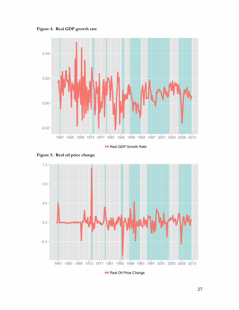
In Figures 4 and 5 in Appendix A, regime 2, is overlaid on real GDP growth rates and real

oil price changes respectively. It is clear that our multivariate MS-VAR model identifies regime 2

based on either occurrences of oil price shocks and oil price volatility, or periods of low and

negative growth rates, or both of these.

Figure 3 reports 1 to 20-step ahead impulse responses of real GDP growth to a 1 standard

deviation shock in the real oil price growth. All impulses are based on Cholesky factor

orthogonalization. Impulse responses are shown in solid and circle symbol lines. The dark grey

regions around the impulse responses correspond to 95 percent confidence intervals. The

confidence intervals for the linear VAR model are obtained from 1,000 bootstrap resampling.

The MS-VAR impulse responses are computed using the regime dependent impulse response

method suggested by Ehrmann, et al. (2003). The confidence intervals for the MS-VAR models

are obtained from the 50,000 posterior draws for each step.

Figure 3(a) and (b) shows that the output growth response to an oil price shock in a high

growth regime is short-lived and the output growth stabilizes to its equilibrium value after 3

quarters. The impact is however statistically insignificant. The impact of an oil shock on output

growth during low growth regimes tends to be posit

persistent with output growth stabilising to its equilibrium value after 8 quarters. The reason

behind the persistence of an oil price shock during the low growth regime could be attributed to

the reaction of monetary authorities. During low growth regimes, which typically also coincides

with recessionary or downswings in the business cycle, the monetary authorities might adopt

expansionary monetary policy, while during high growth regimes, coinciding with upswin

the business cycle, the monetary authority reacts to the increase in oil price by increasing the

interest rate which will harm investment, hence delay the stabilisation of output to its equilibrium

value.

In Figure 3(c), we observe no effect of oil

linear VAR model setting. These show the advantages of nonlinear regime switching models

over the linear alternative, which does not distinguish between the different characteristics under

each regime. The regime dependent IRF allows the asymmetries in terms of the magnitude and

persistence of impact in each regime shown in Figure 3.

Figure 3. Impulse response of GDP to oil price in linear VAR and MS

growth during low growth regimes tends to be positive and significant. The impact is also more



netary authorities. During low growth regimes, which typically also coincides


expansionary monetary policy, while during high growth regimes, coinciding with upswin



In Figure 3(c), we observe no effect of oil price shocks on real output growth under the



me dependent IRF allows the asymmetries in terms of the magnitude and

persistence of impact in each regime shown in Figure 3.

Figure 3. Impulse response of GDP to oil price in linear VAR and MS-VAR models

19

ive and significant. The impact is also more



netary authorities. During low growth regimes, which typically also coincides


expansionary monetary policy, while during high growth regimes, coinciding with upswings in



price shocks on real output growth under the



me dependent IRF allows the asymmetries in terms of the magnitude and

VAR models

20

5. Conclusion

In this paper we have specified and estimated a Bayesian MS-VAR model with a linear VAR as

benchmark, to investigate the role of oil price in different states, or regimes, namely a high

growth–low oil price volatility regime, and a low growth–high oil price volatility regime during

the period 1960Q2 to 2013Q3. Our findings can be summarised as follows: Firstly, the linear

model is rejected in favour of a nonlinear alternative, implying that a regime switching model

exists that characterises the South African business cycle. Secondly, the regime property of the

model shows that the duration of the high growth regime on average is longer compared to that

of low growth regime. Thirdly, we observe that oil price shocks increase the probability to be in

a low growth regime. Using regime-dependent IRFs, we found that the oil price shock tends to

be more persistent during low growth states compared to high growth states, and the impact on

real output growth is also statistically significant. This might be attributed to the asymmetric

reaction of monetary authorities to mitigate the inflationary effect of oil price shocks during low

growth regimes. We furthermore observe that whereas the linear VAR, shows no impact of oil

price shocks on real output growth, the regime-dependent IRFs are able to differentiate between

responses of oil price shocks under each regime, and suggests a significant impact during periods

of low growth.

References

Abeysinghe, T. (2001). Estimation of direct and indirect impact of oil price on growth. Economics Letters, 73(2), 147-153.

Ang, A., Bekaert, G. (2002). International asset allocation with regime shifts. Review of Financial Studies, 15, 1137–1187.

Aye, G. C., Dadam, V., Gupta R., Mamba, B. (2014). Oil price uncertainty and manufacturing production. Energy Economics, 43, 41-47.

Aye, G. C., Gadinabokao, O., Gupta R. (forthcoming). Does the SARB respond to oil price movements? Historical evidence from the frequency domain. Energy Sources, Part B: Economics, Planning, and Policy. Ajmi, A. N., Babalos, V., Gupta, R., Hefer, R. (2014). A Reinvestigation of the Oil Price and Consumer Price Nexus in South Africa: An Asymmetric Causality Approach. Department of Economics, University of Pretoria, Working Paper No. 201423.

21

Blanchard, O. J., Gali, J. (2007). The Macroeconomic effects of oil price shocks: Why are the 2000s so different from the 1970s? National Bureau of Economic Research, NBER Working Paper No. 13368.

Chib, S. (1996). Calculating posterior distributions and modal estimates in Markov mixture models. Journal of Econometrics, 75, 79–97.

Chisadza, C., Dlamini, J., Gupta, R., Modise, M.P. (2013). The impact of oil shocks on the South African Economy. Department of Economics, University of Pretoria, Working Paper Series No. 201311.

Dagut, M. B. (1978). The economic effect of the oil crisis on South Africa. South African Journal of Economics, 46(1), 23-35.

Davies, R. B. (1987). Hypothesis testing when a nuisance parameter is present only under the alternative. Biometrika, 74, 33-43.

De Miguel C., Manzano, B., Martin-Moremo, J. M. (2003). Oil price shocks and aggregate fluctuations. Energy Journal, 24: 47-61.

Dempster, A. P., Laird, N. M., Rubin, D. B. (1977). Maximum likelihood from incomplete data via the EM algorithm. Journal of the Royal Statistical Society Series B, 34, 1-38.

Dickey, D.A., Fuller, W.A. (1979). Distribution of the estimators for autoregressive time series with a unit root. Journal of the American Statistical Association, 74, 427-431.

Diebold, F. X., Lee, J.-H., Weinbach, G. C. (1994). Regime switching with time-varying transition probabilities. In C. Hargreaves (ed.) Nonstationary Time Series Analysis and Cointegration, pp. 283–302, Oxford: Oxford University Press.

Du Plessis, S. A. (2006). Reconsidering the business cycle and stabilisation policies in South Africa. Economic Modelling, 23(5): 761-774.

Durland, J. M., McCurdy, T. H. (1994). Duration-dependent transitions in a Markov model of U.S. GNP growth. Journal of Business and Economic Statistics, 12, 279–288.

Ehrmann, M., Ellison, M., Valla, N. (2003). Regime-dependent impulse response functions in a Markov-switching vector autoregression model. Economics Letters, 78, 295–299.

Elliott, G., Rothenberg, T.J., Stock, J.H. (1996). Efficient tests for an autoregressive unit root. Econometrica, 64, 813–836.

Engemann, K.M., Kliesen, K. L., Owyang, M. T. (2011). Do oil shocks drive business cycles? Some U.S. and international evidence. Macroeconomic Dynamics, 15, 498-517.

Fan, J., Yao, Q. (2003). Nonlinear Time Series: Nonparametric and Parametric Methods. New York: Springer.

Filardo, A. J. (1994). Business-cycle phases and their transitional dynamics. Journal of Business and Economic Statistics, 12, 299–308.

Filardo, A. J., Gordon, S. F. (1998). Business cycle durations. Journal of Econometrics, 85, 99–123.

22

Fruehwirth-Schnatter, S. (2006). Finite Mixture and Markov Switching Models, Statistics. Springer.

Ghysels, E. (1994). On the periodic structure of the business cycle. Journal of Business and Economic Statistics, 12, 289–298.

Granger, C. W. J. (1996). Can we improve the perceived quality of economic forecasts? Journal of Applied Econometrics, 11, 455-473.

Gupta, R., Kanda, P. T. (2014). Does the price of oil help predict inflation in South Africa? Historical Evidence using a frequency domain approach. Department of Economics, University of Pretoria, Working Paper No. 201401.

Hamilton, J.D. (1983). Oil and the macroeconomy since World War II. Journal of Political Economy, 91, 228-248.

Hamilton, J.D. (1988). A neoclassical model of unemployment and the business cycle. Journal of Political Economy, 96, 593-617.

Hamilton, J.D. (1989). A new approach to the economic analysis of nonstationary time series and the business cycle. Econometrica, 57, 357-384.

Hamilton, J. D. (1990). Analysis of time series subject to changes in regime. Journal of Econometrics, 45, 39-70.

Hamilton, J. D. (1994). Time Series Analysis. Princeton, NJ: Princeton University Press.

Hamilton, J.D. (1996). This is what happened to the oil price-macroeconomy relationship. Journal of Monetary Economics, 38(2), 215-220

Hamilton, J.D. (2005). Oil and the macroeconomy. Prepared for: Palgrave Dictionary of Economics.

Hansen, B. E. (2001). The new econometrics of structural change: dating breaks in U.S. labor productivity. The Journal of Economic Perspectives, 15, 117–128.

Herrera, A. N., Lagalo, L.G., Wada, T (2011). Oil price shocks and industrial production: is the relationship Linear? Macroeconomic Dynamics, 15, 472-497.

Johansen, S. (1988). Statistical analysis of cointegration vectors. Journal of Economic Dynamics and Control, 12, 231–254.

Johansen, S. (1991). Estimation and hypothesis testing of cointegration vectors in Gaussian vector autoregressive models. Econometrica, 59, 1551–1580.

Kilian, L. (2009). Not all oil price shocks are alike: Disentangling demand and supply shocks in the crude oil Market, American Economic Review, 99(3), 1053-1069.

Kim, I., Loungani, P. (1992). The role of energy in real Business cycle models. Journal of Monetary Economics, 29, 173-189.

Kim, M.-J., Yoo, J.-S. (1995). New index of coincident indicators: A multivariate Markov switching factor model approach. Journal of Monetary Economics, 36, 607– 630.

23

Krishnamurthy, V., Rydén, T. (1998). Consistent estimation of linear and non-linear autoregressive models with Markov regime. Journal of Time Series Analysis, 19, 291-307.

Krolzig, H.M. (1997). Markov Switching Vector Autoregressions Modelling: Statistical Inference and Application to Business Cycle Analysis. Berlin: Springer.

Krolzig, H.M. (2006). Impulse response analysis in Markov switching vector autoregressive models. Economics Department, University of Kent. Keynes College.

Krolzig, H.M. (2001). Markov-Switching procedures for dating the Euro-Zone Business Cycle, Vierteljahrshelfte zur Wirtschaftsforchung / Quarterly Journal of Economic Research, DIW Berlin, German Institute for Economic Research, 70(3), 3390351.

Krolzig, H.M., Clements, M.P. (2002). Can oil shocks explain asymmetries in the US Business Cycle? Empirical Economics, 27, 185-204.

Kwiatkowski, D., Phillips, P., Schmidt, P., Shin, J. (1992). Testing the null hypothesis of stationarity against the alternative of a unit root. Journal of Econometrics, 54, 159–178.

Lindgren, G. (1978). Markov regime models for mixed distributions and switching regressions. Scandinavian Journal of Statistics, 5, 81-91.

Mork, K. A. (1989). Oil and the macroeconomic when prices go up and down: An extension of hamilton’s results. Journal of Political Economy, 97,740-744.

Nkomo, J C. (2006). The impact of higher oil prices on Southern African Countries. Journal of Energy Research in Southern Africa, 17(1), 10-17.

Ng, S., Perron, P. (2001). Lag length selection and the construction of unit root tests with good size and power. Econometrica, 69, 1519-1554.

Ni, S., Sun, D., Sun, X. (2007). Intrinsic bayesian estimation of vector autoregression impulse responses. Journal of Business and Economic Statistics, 25, 163–176.

Perron, P. (2006). Dealing with structural breaks. Palgrave Handbook of Econometrics 1, 278–352.

Perron, P., Ng, S. (1996). Useful modifications to unit root tests with dependent errors and their local asymptotic properties. Review of Economic Studies, 63, 435-465.

Phillips, P., and Perron, P. (1988). Testing for a unit root in time series regression. Biometrika, 75, 335-346.

Psaradakis, Z. and Spagnolo, N (2003). On the determination of the number of regimes in Markov-Switching Autoregressive Models. Journal of Time Series Analysis, 24, 237–252.

Raymond, J. E., Rich, R. W. (1997). Oil and macroeconomy: A Markov state-switching approach. Journal of Money, Credit and Banking, 29(2), 195-213.

Redner, R. A., Walker, H. (1984). Mixture densities, maximum likelihood and the EM algorithm. SIAM Review, 26, 195–239.

Sims, C. (1980). Macroeconomics and reality. Econometrica, 48, 1–48.

24

Schmidt, T., Zimmermann, T. (2005). Effects of oil prices shocks on German business cycle.

RWI discussion papers No 31.

Tang, W., Wu, L., Zhang, Z. (2010).Oil price shocks and their short- and long-term effects on the Chinese economy. Energy Economics, 32, 3-14.

Zivot, E., Andrews, W. (1992). Further evidence on the great crash, the oil price shock and the unit root hypothesis. Journal of Business and Economic Statistics, 10, 251-270.

25

Appendix A

Table 3. Unit root tests

LROILP LRGDP

Panel A: Unit root tests in levels

ADF -0.7975 [5] -2.1267 [7]

Zα -8.3953 [0] -1.4807 [2]

MZα -8.2175 [0] -1.4167 [2]

MZt -2.014 [0] -0.79409 [2]

DF-GLS -2.0575 [0] -0.7799 [2]

KPSS 1.6308*** [0] 1.3030*** [2]

Zivot-Andrews -4.2794 [5] -3.5118 [7]

Panel B: Unit root test in first differences

ADF -8.4629*** [4] -4.4396*** [6]

Zα -184.07*** [0] -67.232*** [2]

MZα -104.53*** [0] -22.349*** [2]

MZt -7.2153*** [0] -3.3059*** [2]

DF-GLS -12.7050*** [0] -3.9420*** [2]

KPSS 0.0828 [9] 0.5493 [7] Note: Panel A reports unit roots test results for the log levels of the series with a constant and a linear trend in the test equation. Panel B reports unit root test results for the first differences of the log series with only a

constant in the test equation. ADF is the augmented Dickey-Fuller (Dickey and Fuller, 1979) test, Zα is the

Phillips-Perron Zα unit root test (Phillips and Perron, 1988), MZα and MZt are the modified Phillips-Perron tests of Perron and Ng (1996), DF-GLS is the augmented Dickey Fuller test of Elliot, et al. (1996) with generalized least squares (GLS) detrending, KPSS is the Kwiatkowski, et al. (1992) stationarity test, and Zivot-Andres is the endogenous structural break unit root test of Zivot and Andres (1992) with breaks in both the intercept and linear

trend. Zα, MZα, and MZt tests are based on GLS detrending. For the ADF unit root statistic the lag order is selected by sequentially testing the significance of the last lag at 10% significance level. The bandwidth or the lag

order for the MZα, MZt, DF-GLS, and KPSS tests are select using the modified Bayesian Information Criterion (BIC)-based data dependent method of Ng and Perron (2001). ***, ** and * represent significance at the 1%, 5%, and 10% levels, respectively.

26

Table 4. Multivariate cointegration tests

Panel A: VAR order selection criteria

Lag (p) 1 2 3 4 6 8 10

AIC -13.0023 -13.0141 -13.0494 -13.0637 -13.0714 -13.0734 -13.0356

HQ -12.9630 -12.9486 -12.9576 -12.9457 -12.9272 -12.9029 -12.8127

BIC -12.9051 -12.8520 -12.8225 -12.7720 -12.7148 -12.6519 -12.4845

Panel B: Johansen cointegration tests

Eigenvalues 0.0420 0.0360

Critical values Cointegration vector

H0 λmax 10% 5% 1% LROILP LRGDP

r = 1 7.8100 6.5000 8.1800 11.6500 1.0000 1.0000

r = 0 9.1400 12.9100 14.9000 19.1900 -6.5522 -1.0625

Loadings

H0 λtrace 10% 5% 1% LROILP LRGDP

r ≤ 1 7.8100 6.5000 8.1800 11.6500 -0.0033 -0.0625

r = 0 16.9500* 15.6600 17.9500 23.5200 0.0009 -0.0017

Panel C: Stock-Watson cointegration test

H0: q(k,k-r) Statistic Critical values for q(4,3) q(2,0) -1.2029 1% -30.3486

q(2,1) -16.2054 5% -22.8687

10% -19.2077 Note: Table reports selection criteria and multivariate cointegration tests for the VAR(p) model of variables LROILP and LRGDP. Panel A reports the AIC, BIC, and Hannan-Quinn (HQ) information criteria. The VAR

order is selected based on minimum BIC and is 1. Panel B reports maximal eigenvalue (λmax) and trace (λtrace) cointegration order tests of Johansen (1988, 1991). Non-rejection of r=0 for the Johansen tests implies no cointegration. Panel C reports the multivariate cointegration test of Stock and Watson (1988). Under the null q(k,k-r) of Stock-Watson cointegration test, k common stochastic trend is tested against k-r common stochastic trend (or r cointegration relationship). Rejection of q(2,1) for the Stock-Watson test implies cointegration. ***, ** and * represent significance at the 1%, 5%, and 10% levels, respectively.

27

Figure 4. Real GDP growth rate

Figure 5. Real oil price change

the impact of oil price on south african gdp growth: a ... of pretoria department of economics...

Documents