IZA DP No. 1496

The Impact of Parental Income and Educationon the Schooling of Their Children

Arnaud ChevalierColm HarmonVincent O’SullivanIan Walker

DI

SC

US

SI

ON

PA

PE

R S

ER

IE

S

Forschungsinstitutzur Zukunft der ArbeitInstitute for the Studyof Labor

February 2005

The Impact of Parental Income and Education on the Schooling of Their

Children

Arnaud Chevalier University of Kent,

London School of Economics and IZA Bonn

Colm Harmon University College Dublin,

CEPR and IZA Bonn

Vincent O’Sullivan University College London

Ian Walker

University of Warwick, Institute of Fiscal Studies and IZA Bonn

Discussion Paper No. 1496 February 2005

IZA

P.O. Box 7240 53072 Bonn

Germany

Phone: +49-228-3894-0 Fax: +49-228-3894-180

Email: iza@iza.org

Any opinions expressed here are those of the author(s) and not those of the institute. Research disseminated by IZA may include views on policy, but the institute itself takes no institutional policy positions. The Institute for the Study of Labor (IZA) in Bonn is a local and virtual international research center and a place of communication between science, politics and business. IZA is an independent nonprofit company supported by Deutsche Post World Net. The center is associated with the University of Bonn and offers a stimulating research environment through its research networks, research support, and visitors and doctoral programs. IZA engages in (i) original and internationally competitive research in all fields of labor economics, (ii) development of policy concepts, and (iii) dissemination of research results and concepts to the interested public. IZA Discussion Papers often represent preliminary work and are circulated to encourage discussion. Citation of such a paper should account for its provisional character. A revised version may be available directly from the author.

IZA Discussion Paper No. 1496 February 2005

ABSTRACT

The Impact of Parental Income and Education on the Schooling of Their Children∗

This paper addresses the intergeneration transmission of education and investigates the extent to which early school leaving (at age 16) may be due to variations in permanent income, parental education levels, and shocks to income at this age. Least squares estimation reveals conventional results - stronger effects of maternal education than paternal, and stronger effects on sons than daughters. We find that the education effects remain significant even when household income is included. Moreover, decomposing the income when the child is 16 between a permanent component and shocks to income at age 16 only the latter is significant. It would appear that education is an important input even when we control for permanent income but that credit constraints at age 16 are also influential. However, when we use instrumental variable methods to simultaneously account for the endogeneity of parental education and paternal income, we find that the strong effects of parental education become insignificant and permanent income matters much more, while the effects of shocks to household income at 16 remain important. A similar pattern of results are reflected in the main measure of scholastic achievement at age 16. These findings have important implications for the design of policies aimed at encouraging pupils to remain in school longer. JEL Classification: I20, J62 Keywords: early school leaving, intergenerational transmission Corresponding author: Colm Harmon Geary Institute University College Dublin Belfield, Dublin 4 Ireland Email: colm.harmon@ucd.ie

∗ This paper forms part of the UCD Geary Institute’s Policy Evaluation programme. Chevalier and Walker are also affiliated with the Centre for the Economics of Education (CEE) at the London School of Economics. The support of CEE in facilitating this collaboration is gratefully acknowledged. Financial support from the HM Treasury Evidence Based Policy programme, the Nuffield Foundation Small Grant Scheme and the award of a Nuffield Foundation New Career Development Fellowship to Harmon is also gratefully acknowledged. We thank Tarja Viitanen for able research assistance, and we are grateful to Pedro Carneiro, Kevin Denny and seminar participants at CEMFI in Madrid, RAND in Santa Monica, the University of Glasgow, and the Tinbergen Institute for comments. The data used in this paper was made available by the UK Data Archive at the University of Essex.

1. Introduction A considerable literature has focused on the effects of parental background on such outcomes

for their children as cognitive skills, education, health and subsequent income (see, for

example, Jere R. Behrman, 1997). There is little doubt that economic status is positively

correlated across generations. Parents, and the family environment in general, have important

impacts on the behavior and decisions taken by adolescents.

The view that more educated parents provide a “better” environment for their children

has been the basis of many interventions. Moreover, while the scientific literature is not so

clear, it is widely believed that while raising the education for mothers and fathers has

broadly similar effects on household income, the external effects associated with education is

larger for maternal education than for paternal because mothers tends to be the main provider

of care within the household. For example, a positive relationship between mother’s

education and child birth weight, which is a strong predictor of child health, is found not only

in the developing world but also in the US (see, for example, Janet Currie and Enrico Moretti,

2003). The existence of such externalities provides an important argument for subsidizing

the education of children, especially in households with low income and/or low educated

parents. Indeed there may be multiplier effects since policy interventions that increase

educational attainment for one generation may spillover onto later generations.

While the existence of intergenerational correlations is not disputed, the nature of the

policy interventions that are suggested depends critically on the characteristics of the

intergenerational transmission mechanism and the extent to which the correlation is causal.

In particular, is has proved difficult to determine whether the transmission mechanism works

through inherited genetic factors or environmental factors and, if it is the latter, what is the

relative importance of education and income. For example, ability is positively associated

with more schooling and ability may be partly transmitted from parents to children1. The

link, therefore, between the schooling of parents and their children could be due to

unobserved inherited characteristics rather than a causal effect of parental education per se in

household production. A related issue is the extent to which any causal effect of education

1 Taking IQ as a measure of ability, the correlation in IQ between parents and natural children is 0.42 for children living with their parents and 0.22 for those brought up apart (see Marcus W. Feldman et al , 2000).

1

works through the additional household income associated with higher levels of education.

That is, parental educations may be both direct inputs into the production function that

generates child quality and may indirectly facilitate a higher quantity of other inputs through

the effect of educational levels on household income.

This paper addresses two major issues in the existing literature: the causal effect of

parental education on children, allowing for separate effects of mother’s and father’s

education; and the causal effect of household income. To date no study has simultaneously

tried to account for both the endogeneity of parental education and of income. This is a

crucial distinction since important policy differences hang on their relative effects. A further

important innovation of this paper is that, in addition to controlling for both income and

education, we try to decompose the effects of income into permanent and transitory elements.

The motivation for the former is that a policy might be concerned with providing financial

transfers to households holding parental education levels constant – for example income

support policies aimed at relieving child poverty. The importance of the latter innovation is

that we need to distinguish credit constraints at the point of decision to enter post-compulsory

schooling from the permanent effects of long term income differences so as to inform policy.

Using a British dataset, we begin by confirming the usual finding using OLS - that

parental education levels are positively associated with good child outcomes by looking, in

particular, at early school leaving decisions. We go on to investigate the relative effects of

parental education levels and household income on early school leaving and achievement at

age 16 (measured as the number of GCSE qualifications obtained at the passing grades of A

to C). These two measures are important because the present government has targeted a

reduction in the proportion of pupils leaving at 16, and because the number of GCSE passes

is influential in determining one’s opportunities for post-compulsory study. We go on to use

instrumental variable methods to take account of the endogeneity of both parental income and

education. Finally we exploit the rotating panel aspect of our dataset to identify transitory

and permanent income. The plan of the paper is as follows. Section 2 outlines the existing

literature. Section 3 explains the nature of the data used. Section 4 provides the base

estimates which are extended in Section 5 to separate permanent and transitory effect of

paternal income, as well as focusing on GCSE score rather than schooling decision at 16.

Section 5 concludes.

2

2. Previous Literature

A number of studies have found a strong link between earnings of the parent (typically the

father) and of the child with the intergenerational correlation in earnings between fathers and

sons between 0.40 and 0.50 in the US and 0.60 in the UK. There is also a relationship

between parental education and the education of their offspring. Estimates of the elasticity

for intergenerational mobility in education lie between 0.14 to 0.45 in the US and 0.25 to 0.40

in the UK (see Lorraine Dearden et al. (1997) for the UK, and Casey Mulligan (1999) and

Gary Solon (1999) for the US).

Children brought up in less favorable conditions obtain less education despite the

large financial returns to schooling (see James J. Heckman and Dimitry Masterov (2004) for

an extensive review). However the mechanism by which such intergenerational correlations

are transmitted is not clear. Alan B. Krueger (2004) reviews various contributions supporting

the view that financial constraints significantly impact on educational attainment. On the

contrary, Pedro Carneiro and Heckman (2003) suggests that current parental income does not

explain child educational choices but that family fixed effects such as parental education

levels, that contributes to permanent income, have a much more positive role. This is the

central conclusion of Stephen Cameron and Heckman (1998) using US data, and Arnaud

Chevalier and Gauthier Lanot (2002) using the UK National Child Development Study data.

Chevalier (2004), using the Family Resources Survey cross-section data, finds that including

father’s income in the schooling choice equation of the child, while itself a significant and

positive effect, does not dramatically change the magnitude of the parental education

coefficients. However, the potential endogeneity of income means that this correlation does

not necessarily imply that parental income matters for children’s human capital accumulation.

Indeed if income is endogenous and is correlated with education, then the education

coefficients are also biased.

So far, researchers have been able to identify the exogenous effect of parental

education or income but not both effects simultaneously. The literature on estimating the

causal effect of parental education on the child’s educational attainment has relied on three

identification strategies. Behrman and Mark Rosenzweig (2002) use the Minnesota Twins

Register to examine educational choice of children of twin pairings (who are therefore

cousins) to eliminate the nature effect of one of the parents. Based on simple OLS models,

they find large effects: one year of maternal schooling increased children’s years of education

3

by 13% while the effect of paternal schooling was about twice as large. However between-

cousins estimates of maternal education effects are negative albeit insignificant. This

contradicts the general view that maternal schooling has a larger and positive effect than

paternal schooling on the achievement of their children2.

An alternative strategy to account for genetic effects is to compare adopted and

natural children. Both Bruce Sacerdote (2002) and Erik Plug (2003) report that, controlling

for ability and assortative mating, the positive effect of maternal education on children’s

education disappears. This literature assumes that the presence of adopted children is

uncorrelated with unobservables across families. However adopted and natural children may

have different characteristics, be treated differently in school or by society (especially when

of different race from their parents), or may have incurred some stigma from adoption.

Additionally, adoptive families may provide a different environment to children such as more

(or less) attention to the child. As evidence of differences in the environment of adopted and

natural children, Barbara Maughan et al (1998) find that adoptees performed more positively

than non-adopted children from similar families on childhood tests of reading, mathematics,

and general ability. In contrast, Anders Bjorklund et al. (2004) uses a register of Swedish

adoptees which confirms the findings of studies such as Plug (2003) and when correcting for

the potential bias caused by non-randomness in this population they find that genetics

account for about 50% of the correlation in education between generations but that after

accounting for genetics, the causal effects of parental education remains highly significant.

The third identification strategy is to use instrumental variables methods based on

‘natural’ experiments or policy reforms which change the educational distribution of the

parents without directly affecting children. Sandra E. Black et al. (2003) exploit Norwegian

educational reforms which raised the minimum number of years of compulsory schooling

over a period of time and at differential rates between regions of the country. They find

evidence of parental impact in the OLS estimates of education outcomes for the children but

estimates based on IV do not show this effect, with the exception of (weak) evidence of

2 In a critical analysis of the Behrman and Rosenzweig (2002) data, Karen Antonovics and Arthur Goldberger (2004) show that results are quite sensitive to the selection of children who have completed education and who are aged 18 and over, rather than 16 and over. Behrman, Rosenzweig and Junsen Zhang (2004) repeat the original analysis on a large Chinese dataset and find strong support for their earlier analysis.

4

mother/son influences. However, Philip Oreopoulos et al. (2003) using the same approach

and pooling US Census data from 1960, 1970 and 1980 report that an increase in parental

education by one year decreases the probability of repeating a schooling year (or grade) by

between two and seven percentage points.

The UK provides similar policy changes which are exploited in Chevalier (2004) and

Fernando Galindo-Rueda (2003). Changes in the minimum school leaving age which

occurred just after World War II and in the early 1970s meant that the educational choice of

parents was exogenously affected, at least for those wishing to leave school at the earliest

age. Some parents experienced an extra year of education compared to other parents who

were similar to them in other respects except birth year. This discontinuity is exploited to

identify the effect of parental education on their children’s education. Chevalier (2004) finds

that for both parents, OLS estimates of the effect of one year of parental education on the

probability of post-compulsory education is about 4%, with the effects slightly larger for sons

than daughters. Using the 1974 change in the school leaving age legislation as an instrument

for parental education, the effects of a parent’s education on the child of the same gender

increased substantially (for a sample of natural parents). Galindo-Rueda (2003) exploited the

earlier 1947 reform and, relying on regression discontinuity, find significant causal effect but

only for fathers.

The literature on the causal effects of parental earnings or incomes on educational

outcomes is not extensive. Random assignment experiments are potentially informative but

uncommon. Jo Blanden and Paul Gregg (2004) review US and UK evidence on the

effectiveness of policy experiments which largely focus on improving short term family

finances. These include initiatives such as the Moving to Opportunity (MTO) experiments in

the US which provide financial support associated with higher housing costs from moving to

more affluent areas. MTO programs are associated with noticeable improvements in child

behavior and test scores but whether these are caused by the financial gain or the

environment, school and peer-group changes is unclear3. In the UK, the pilots of Educational

Maintenance Allowances (EMA’s) provided a sizeable means tested cash benefit conditional

3 Note that new work on MTO by Lisa Sanbonmatsu et al (2004) suggests that MTO-driven neighbourhood effects on academic achievement were not significant.

5

on participation in education and paid, depending on pilot scheme, either to the parents or

directly to the child (UK Department for Education and Skill, 2002). Enrollments increased

by up to 6% in families eligible for full subsidies. However, this transfer was conditional on

staying in school and so does not tell us about the effects of unconditional variations in

income.

In the absence of experimental evidence, instruments have been used to identify

income effects. John Shea (2000) uses union status (and occupation) as an instrument for

parental income and therefore assumes that unionized fathers are not more ‘able’ parents than

nonunion fathers with similar observable skills, while Bruce Meyer (1997) uses variation in

family income caused by state welfare rules, income sources and income before and after the

education period of the child, as well as changes in income inequality. While strong

identification assumptions are used in both these studies, they both find that unanticipated

changes in parental long-run income have modest and sometimes negligible effects on the

human capital of the children4. Using UK data, Blanden and Gregg (2004) find the

correlation between family income and children’s educational attainment has actually risen

between the 1970 birth cohort data and the later British Household Panel Survey data

containing children reaching 16 in the late 1990’s. They estimate the causal effect of family

income in ordered probit models of educational attainment (from no qualifications up to

degree level) based on sibling differences in the panel data. They also provide estimates of

the probability of staying-on at school past the minimum age of 16. However the paper

cannot simultaneously provide estimates of the causal effect of parental education because

this is treated as a fixed effect in the sibling difference estimates and so differences out.

Finally, Stephen Jenkins and Christian Schluter (2002) is notable for being one of the few

studies to control both for income at various ages and education. Using a small German

dataset to study the type of school attended (vocational or academic) they find that later

income is more important than early income, but that income effects are small relative to

education effects. The analysis in their paper, as in Blanden and Gregg (2004), assumes the

4 Daron Acemoglu and Jorn-Steffan Pishke (2001) use similar arguments to Meyer (1997) and exploit changes in the family income distribution between the 1970’s and 1990’s. They find a 10 percent increase in family income is associated with a 1.4% increase in the probability of attending a four year college.

6

exogeneity of income and parental education. Here, we follow Shea (2000) in using union

status as an instrument for income.

3. Data and Sample Selection

To carry out this research, data on two generations are required in a single data source –

education of the individual children and the education and incomes of their parents. Our

analysis is based on the Labour Force Survey (LFS) which is a quarterly sample of

households in the U.K. In each quarter there are roughly 138 thousand respondents from the

approximately 59 thousand households surveyed. Households are surveyed for five

consecutive quarters. We pool the data from households in the fifth quarter over the period

1993-20035. Children aged 16 to 18 living at home are interviewed in the LFS so parental

information can be matched to the child’s record6. Our sub-sample consists of those children

observed in LFS at ages 16 to 18 inclusive (and therefore have made their decision with

respect to post compulsory education participation).

The key outcomes of interest in this paper are the decisions to participate in post-

compulsory schooling, and the achievement of five or more GCSEs (at grades A to C). The

latter is a requirement to continue in education for many schools, and a necessary condition

for admission to university (together with having two or more A-Level passes in

examinations taken at age 18). For the former outcome we define a dummy equal to one if

the 16 to 18 year old child is either in post compulsory education at present or was in

education between 16 and 18 but has left school at the time of interview (based on the age left

full time education information in LFS). For the latter we also define a dummy variable

based on the achievement of the required GCSE standards7.

5 Pre-1998, earnings data is available only for fifth wave respondents, post 1998, the earnings data is collected in the first and in the final wave. 6 Chevalier (2004) uses the Family Resource Survey data which in many respects is similar to the LFS data in this paper but allow to distinguish between natural and step parents which is not possible with the LFS, therefore parents in our study could be natural, step or foster parents. The LFS on the other hand has information on union status which is crucial for the identification strategy adopted in this paper. 7 27% of all those aged 16-19 do not report the number of GCSE’s received. Of that group 95% report having no qualifications or qualifications below the level of five GCSE A-C grades and were therefore recoded as having failed to achieve this level.

7

The age range is limited because we need to observe respondents while they are still

living at home in order to observe their parent’s education levels (respondents are not asked

directly about the education of their parents). We only select teenagers where both parents

are present to avoid some heterogeneity that would be hard to model8. This represents 94%

of children aged 16-18. However, the selection becomes more severe with older teenagers -

whilst 98% of 16 year old children are observed living with both parents, this proportion in

down to 88% for those 18 years old.

We select teenagers where the father is working and reporting his income, where both

parents were born after 1933 (and so were not affected by the earlier raising of the school

leaving from 14 to 15), and where parents were born in the United Kingdom (or immigrated

at a very young age). We also drop any observations where there is missing data. Full

details on the original LFS data and the impact of the selection criteria can be seen in

Appendix Table A1.

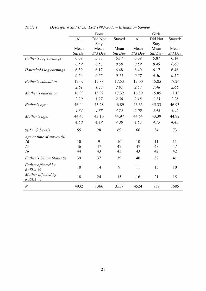
Table 1 shows some selected statistics for the sub-sample used in our analysis. The

staying on rate is 72% for boys and 81% for girls. 69% (73%) of boy (girl) stayers have 5+

GCSE qualifications compared to 28% (34%) of leavers9. There are large differences in the

parental education and household income levels between those that remain in school

compared to those that leave. The differences in paternal union status between those that

stayed past 16 and those that left is small. The union earnings gap in the raw data is 10%.

Figures 1a and 1b shows the participation rate in post-compulsory schooling in our

final sample broken down by paternal and maternal education. The education of the children

appears closely correlated with the education of their parents. The relationships are steep up

to a leaving age of 18; whilst having parents with more education than this level does not

substantially affect the staying-on probability of children. There are some sizable gaps

8 Whilst this may create some selection bias it would be difficult to overcome this in our data. Since separation is more likely for children with unobservably large propensities to leave school early, and it is negatively correlated with parental education and income we might expect to underestimate the effect of income and education on the dependent variables. 9 Official statistics from the Department for Education and Skills show 67% of boys and 75% of girls in the relevant cohort choosing to stay so our staying-on figures from LFS are a little higher. Some 48% of pupils achieved 5+ GCSE qualifications at grade A*-C in 1998, slightly lower than in our data.

8

between the participation of girls and boys from lower educated parents but this gap narrows

with parental education. Figures 2a and 2b show similar patterns for the proportion

achieving five or more GCSE passing grades.

4. Estimates

Our basic model of the impact of parental background on their children is:

(1) 1 2 3

1 2 3

( , , )

( , , )

pcc m p p h c m p c

Gc m p p h c m p c

PC S S Y X f DB DB DB

G S S Y X g DB DB DB

β β β δ ε

α α α φ ε

= + + + + +

= + + + + +

where the c, m and p subscripts refer to the child, maternal and paternal characteristics within

a particular household h. The dependent variable PCc is a dummy variable defining

participation in post compulsory education. The dependent variable Gc is the dummy

variable for whether or not the child had attained five or more GCSE passing grades. These

are estimated as linear probability models, to facilitate the use of instrumental variables, and

are functions of parental education measured in years of schooling of both the mother and

father (Sm , Sp) and parental income Yp measured by father’s real log gross weekly earnings

from employment10. DB refers to date of birth (year and month) so that f(.) and g(.) controls

for trends in paternal, maternal and child education. Finally Xh contains characteristics

common to all three members of the family (i.e. year and month of survey dummies as well

as region of residence at time of survey).

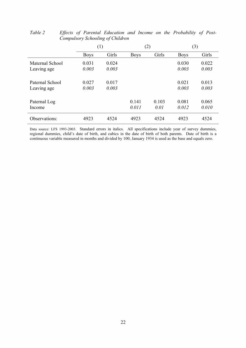
Table 2 summarizes our estimates of parental education and income on the probability

of post-compulsory schooling of the child11. Specification (1) only controls for parental years

of schooling and suggests positive, if modest, paternal and maternal education effects on the

schooling choice of both sexes. The impact of a year of maternal education is an increase in

10 Note that we use paternal income because the use of household income measures requires the inclusion of female earnings which is potentially much more heavily affected by endogenous labour supply decisions. However its exclusion may also cause a bias if female labour supply is correlated with educational outcomes for children as well as with the variable of interest in the model. We share our inability to resolve this problem with the rest of the literature. If maternal labour supply is uncorrelated with paternal income and if incomes are shared within the household then our estimate of the effect of paternal income is the same as the effect of household income. This is clearly an important problem for future research. 11 Full results available on request. Similar estimates based on probit models are also available. While multiple observations of closely spaced children in each household are possible their incidence is small (10% of individuals have at least one other sibling in the dataset) and any improvement in standard errors from exploiting the clustering in the data would be marginal.

9

the probability of post-16 participation of about 4% for boys and 3% for girls – about 1%

lower than reported in Chevalier (2004). The impact of paternal education is slightly lower

and the effect on boys is larger than for girls. Specification (2) examines the impact of

paternal income but excludes the parental education controls. These estimates suggest

sizable and significant income elasticities with the effect slightly larger for boys (15%) than

for girls (10%). Finally specification (3) includes both education and income controls. The

direct effects of education estimated in Specification (1) are reduced slightly in (3) but the

income effect is effectively halved in this specification. The estimated income effects here are

closely comparable in magnitude to the results in Blanden and Gregg (2004)12.

As already discussed the impact of parental schooling and income on education

outcomes of children may suffer from endogeneity problems. In this paper we identify the

effect of parental education on children’s education using the exogenous variation in

schooling caused by the raising of the minimum school leaving age (RoSLA). Individuals

born before September 1957 (or, for Scotland, September 1960) could leave school at 15

while those born after this date had to stay for an extra year of schooling. This policy change

creates a discontinuity in the years of education attained by the parents. Figure 3 illustrates

this by showing mean years of schooling by birth year and month for the period around the

reform date. There is a marked jump in the graph for parents born in September 1957 which

coincides with the introduction of the new school leaving age. Individuals affected by the

new school leaving age have on average completed half a year more schooling than those

born just before the reform. Chevalier et al. (2004) show that the effect of this reform was

almost entirely confined to the probability of leaving at 15.

Parental income is also potentially endogenous either because correlated with

unobservable characteristics explaining educational performance, or because the parental

education effect is through income. We identify parental income effects from the union

status of the father. We assume that union status creates an exogenous change in income

which is independent of parenting ability and the child’s educational choice. Indeed the raw

data, presented in Table 1, showed that children who stay on are just as likely to have

unionized fathers as children who do not stay on in education. H.Gregg Lewis (1986), and

12 See their Tables 6 and 7 in particular.

10

much subsequent work, demonstrates that wages vary substantially with union status,

controlling for observable skills. If union wage premia reflect rents rather than unobserved

ability differences it seems plausible to make the identifying assumption, used in this paper;

that union status is uncorrelated directly with the parental influence on educational outcomes

of the children. Support for the view that unionization picks up differences in labor market

productivity is mixed. Kevin Murphy and Robert Topel (1990) find that individuals who

switch union status experience wage changes that are small relative to the corresponding

cross-section wage differences, suggesting that union premia are primarily due to differences

in unobserved ability. However Richard Freeman (1994) counters this view, arguing that

union switches in panel data are largely spurious so that measurement error biases the union

coefficient towards zero in the panel. In any event, we are assuming, as in Shea (2000), that

unionized fathers (and their spouses) are not more ‘able’ parents than nonunion fathers with

similar observable skills.

Dummy variables for RoSLA and union status are incorporated into the model. We

therefore estimate the following system of first stage equations:

(2) 1 2

1 2

1 2 3

( )

( )

( )

m m h m m

p p h p p

p p p h p p

S RoSLA X r DB

S RoSLA X s DB

Y UNION S X t DB

φ φ µθ θ υ

π π π ω

= + + +

= + + +

= + + + +

where the functions r(.), s(.), and t(.) control for smooth trends in school leaving so that the

RoSLA dummy variables just pick up the effects of the reform. The top portion of Table 3

presents the first stage regressions for paternal and maternal education, and paternal earnings,

with the schooling equations estimated separately from the earnings equation. The RoSLA

variables are significant (although marginally so in the case of the fathers) and positive in

both of the parental schooling equations. The paternal earnings equation shows a significant

positive union membership wage premium and rates of returns to schooling consistent with

existing UK evidence. The bottom half of Table 3 estimates these equations simultaneously

using the seemingly unrelated regression method. A number of noticeable changes occur.

While they are still significant the RoSLA dummy for the father is reduced in this

simultaneous estimation. The earnings function shows a similar premium for union status.

However the impact of education rises dramatically to almost 25%. This estimate is

significantly larger than even those based on using school leaving age reforms as an

instrument (Colm Harmon and Ian Walker, 1995). Our interpretation of this estimate is that it

11

is a Local Average Treatment Effect associated with forcing those that left school at 15 to

take an extra year of education and the subsequent estimates should be interpreted with that

in mind13.

Table 4 repeats the specification shown in Table 2 but parental educations and

paternal income are treated as endogenous14. We estimated fitted values for the key variables

from the first stage regressions in Table 3. The basic results from Table 2 now change

considerably. In specification (1) where earnings measures are not included the parental

education variable are largely insignificant with only the impact of mother’s education on

daughters being close to significant. The impact of parental income in the second

specification suggests sizable income elasticities with a doubling of paternal income

increasing the probability of post-compulsory schooling of sons by 50% and of daughters by

34%. The income effect is more than halved when we reintroduce our parental education

variables in the third specification but the impact of parental education is still largely

insignificant. If we believe that this strategy, which relies on the exogenous component of

union status on income, identifies the permanent effect of income, the results are not

dissimilar to Carneiro and Heckman (2003).

It is possible that our results are contaminated by omitted ability. Extensive ability

tests were conducted in National Child Development Study, a longitudinal dataset following

children born in the UK during a given week of 1958, so we attempt to replicate Tables 2 and

4 using this data to investigate the extent of this problem. The results are reported in Table 5.

Note that the NCDS results which exclude ability and the LFS results are also similar despite

the fact that in the NCDS data we exploit the 1947 policy change, which raised the minimum

school leaving age from 14 to 15, to provide and instrument. The important result to take

away from Table 5 is that the NCDS estimates of income and education effects are hardly

changed by the inclusion of the test scores. However, it is not possible to simultaneously

account for the endogeneity of parental education and income in the NCDS as the union

status of the father is not reported.

13 Estimates of the paternal log income equation that use dummy variables for each year of education (not reported here) show the nonlinearity of returns with individuals leaving school at 16, 17, 18 and 20 having large returns to their educational investment. Returns to education past the age of 21 appear rather flat.

12

A major unresolved issue in the literature is the extent to which parental incomes

affect outcomes for children through short run considerations, such as relieving credit

constraints, as opposed to through long run permanent effects. In the UK, Dearden et al

(2004) address the issue of credit constraints using the British Cohort Studies of 1970 (and

the earlier NCDS) data and investigate the relationship between early school leaving and

parental incomes. They find, using least squares, that there are current income effects even

when controls for ability and parental background like education are controlled for which

they presume capture credit constraints. However, Chevalier and Lanot (2002) report that

income effects are dwarfed by permanent family characteristics.

We also are interested in the effect of transitory income shocks when the child is 16.

The LFS data that we have used so far has included children aged 16 to 18. From 1998

onwards, LFS has included earnings information in both first wave and the last wave of the

survey. Prior to this date earnings information was only recorded for the outgoing rotation.

Having one earnings observation allows us to estimate an earnings function and compare the

actual wage outcome with predicted to compute the shock when the child is 16, for those

observations that contain a child aged 16 in wave 5. Having two observations on earnings

allows us to use data on households that contain a child aged 15 in wave 1 (and hence 16 in

wave 5 as before) as well as households with a child aged 16 in wave 1 (and hence 17 in

wave 5). In the first case we can compute the residual directly while in the second case we

can compute the residual when the child is aged 16 by ageing the parents back one year and

predicting what they would have earned when the child was 16 in wave 1. Thus we can

continue to use data from 1993 onwards, provided the child is 16 in wave 5, and we can

supplement this by households from 1998 onwards who have a child aged 16 in wave 1. We

can then capture the distinction between permanent and transitory elements of earnings by

including both the predicted earnings and its residual.

The results in Table 6 take the specifications in Tables 2 and 4 and further include the

residual from the earnings function. Specification (1) in Table 6 assumes that all variables are

exogenous and correspond to Table 2; while specification (2) assumes that parental education

and permanent income are endogenous and so corresponds to Table 4. The results here

14 We use the SUR first stage results from Table 3 to correct for the endogeneity. Estimates that use estimates of

13

suggest that permanent income is insignificant and education effects are significant when

they are assumed to be exogenous but there does seem to be some support for the notion that

credit rationing may be a factor. However, in specification (2), allowing for the endogeneity

of education and permanent income, we find that education is no longer significant but

permanent income now appears to be so, while some credit rationing is still in evidence15.

Table 7 shows the determinants of scholastic success measured by having 5 or more

GCSE at grades higher than D. As this measure reflects long-term effort and does not have

financial implication, in the way that the decision to remain post compulsory education has,

the effect of permanent income is ambiguous whilst transitory income shocks are likely to

have only a small impact. It contrasts the importance of education and income in the case

where these are treated as exogenous with the unimportance of education when both as

treated as endogenous. When education and income are assumed exogenous these results also

suggest that parental education levels are important and that, despite their correlation,

education remains important when income is also included. When both are regarded as

endogenous we find, as with the early school leaving results, education is no longer

significant but income is16. Table 8 replicates the model presented in Table 6 but now the

outcome of interest is our measure of scholastic success: having more than 5 GCSE at grades

A to C. In the exogenous model, maternal education matters and so do shocks in earnings,

whilst surprisingly, the permanent income has a significant effect for boys only. However,

when we used instrumental variable methods we found that the strong effects of parental

education became insignificant and permanent income mattered much more, while the effects

of shocks to household income at 16 remained important. A similar pattern of results were

reflected in the decision to remain in post-compulsory schooling, surprisingly we find that

shocks at age 16 are also significant for GCSE performance, maybe because the incentives to

perform well at the test, and therefore continues beyond compulsory schooling, is reduced for

individuals affected by a negative shock.

the income and education equations separately show little difference and are available on request. 15 The results in Tables 2 and 4 are essentially unchanged if we use this smaller sample. Results are available on request. We also split this sample into 16 year olds, for whom we are forecasting forward, and 17-year olds, who we are forecasting backwards. We lose precision in doing this and the results are not significantly different from those in Table 6.

14

5. Conclusion

This paper has addressed the intergenerational transmission of education and investigated the

extent to which early school leaving (at age 16) may be due to variations in permanent

income, parental education levels, or shocks in income at this age. Least squares revealed

conventional results - stronger effects of maternal education than paternal, and stronger

effects on sons than daughters. We also found that the education effects remained significant

even when household income was included. Moreover, when parental education was included

we found that permanent income was insignificant while shocks to income at age 16

remained significant. Similar results were found when looking at scholastic achievement

rather than the decision to stay-on.

The IV results contrast strongly with some earlier US work: it would appear that

education does not have an independent effect when we control for exogenous variation in

permanent income, and that permanent income remains important even when we allow for an

impact of credit constraints at age 16. The implications for policy are that some policy to

relieve credit constraints at the minimum school leaving age, say through an Educational

Maintenance Allowance (see DfES (2002)), would be effective in promoting higher levels of

education. And a policy of increasing permanent income, say through Child Benefit would

also be effective. However, any claim that an EMA will benefit future generations through

direct intergenerational transmission seem doubtful. Similar results apply for GCSE success.

Further work is needed in several areas. Most notably, it would be interesting to

estimate the effects on the probability of obtaining 5+ GCSE passes and the probability of

staying jointly – that is, allow for the direct effect of scholastic success on staying on. This

would allow a more detailed investigation of the transmission mechanism that included the

extent to which permanent income mattered for staying on because it mattered for GCSE

success.

16 Independent regressions of post-compulsory schooling and obtaining 5 or more GCSE Grades A-C produce the same results as here and there is some gain in precision from exploiting the covariances between the two outcomes, shown in Appendix Table A2.

15

References

Acemoglu, Daron. and Pischke, Jorn-Steffan. “Changes in the Wage Structure, Family Income and Children’s Education.” European Economic Review, 2001, 45, pp. 890–904.

Antonivics, Karen and Goldberger, Arthur. “Does Increasing Women’s Schooling Raise the Schooling of the Next Generation? Comment.” forthcoming American Economic Review, 2004

Behrman, Jere. “Mother’s Schooling and Child Education: A Survey.” University of Pennsylvania Department of Economics, DP 025, 1997.

Behrman Jere and Rosenzweig, Mark. “Does Increasing Women’s Schooling Raise the Schooling of the Next Generation.” American Economic Review, 2002, 92, pp. 323-334

Behrman Jere, Rosenzweig, Mark and Zhang, J. “Does increasing women’s schooling raise the schooling of the next generation. Reply”, forthcoming, American Economic Review, 2004.

Bjorkland, Anders, Lindahl, Mikael and Plug, Erik. “Intergenerational Effects in Sweden: What Can We Learn from Adoption Data?” IZA Discussion Paper 1194, 2004.

Black, Sandra E., Devereux, Paul J. and Salvanes, K.G. “Why the Apple Doesn't Fall Far: Understanding Intergenerational Transmission of Human Capital.” IZA Discussion Paper 926, 2003.

Blanden, Jo and Gregg, Paul. “Family Income and Educational Attainment: A Review of Approaches and Evidence for the UK.” University of Bristol, Centre for Market and Public Organisation Working Paper 04/101, 2004

Cameron Stephen and Heckman, James J. “Life Cycle Schooling and Dynamic Selection Bias: Models and Evidence for Five Cohorts of American Males”, Journal of Political Economy, 1998, 106, pp. 262-333

Carneiro Pedro and Heckman, James J. “Human Capital Policy.” National Bureau of Economic Research, Working Paper 9495, 2003.

Chevalier, Arnaud. “Parental Education and Child's Education: A Natural Experiment”, IZA Discussion Paper no. 1153, 2004.

Chevalier Arnaud, Harmon, Colm, Walker, Ian and Zhu, Yu. “Does Education Raise Productivity or Just Reflect It?”, Economic Journal, 2004, 114, pp. F499-F517.

Chevalier Arnaud and Lanot, Gauthier. “The Relative Effect of Family Characteristics and Financial Situation on Educational Achievement.” Education Economics, 2002, 10, pp. 165-182

Currie, Janet and Moretti, Enrico. “Mother’s Education and the Intergenerational Transmission of Human Capital: Evidence from College Openings and Longitudinal Data”, Quarterly Journal of Economics, 2003, 118, pp. 1495-1532

Dearden, Lorraine. “Credit Constraints and Returns to the Marginal Learner”, Institute for Fiscal Studies, mimeo, 2004.

Dearden Lorraine, Machin, Stephen and Reed, Howard. “Intergenerational Mobility in Britain”, Economic Journal, 1997, 107 (1), pp. 47-66.

16

Feldman Marcus W., Otto, Sarah P. and Christiansen, Freddy B. “Genes, culture and inequality” in Kenneth Arrow, Samuel Bowles and Steven Durlauf, eds., Meritocracy and Economic Inequality. 2000, Princeton: Princeton University Press.

Freeman, Richard B. “H.G. Lewis and the Study of Union Wage Effects”, Journal of Labor Economics, 1994, 12, pp. 143-149.

Galindo-Rueda, Fernando. “The Intergenerational Effect of Parental Schooling: Evidence from the British 1947 School Leaving Age Reform.” Centre for Economic Performance, London School of Economics, mimeo, 2003.

Gregg, Paul, Harkness, Susan and Machin, Stephen. “Poor Kids: Child Poverty in Britain, 1966-1996.” Fiscal Studies, 1999, 20, pp. 163-187.

Harmon Colm and Walker, Ian. “Estimates of the Economic Return to Schooling in the United Kingdom”, American Economic Review, 1995, 85, pp. 1278-1286.

Heckman, James J. and Masterov, Dimitri V. “Skills Policies for Scotland”, University of Chicago, mimeo, 2004.

Imbens Guido and Angrist Joshua. “Identification and Estimation of Local Average Treatment Effects”, Econometrica, 1994, 62, pp. 467-475

Jenkins, Stephen P. and Schluter, Christian. “The Effect of Family Income During Childhood on Later-Life Attainment: Evidence from Germany.” 2002, DIW Discussion Paper 317.

Krueger, Alan B. “Inequality, Too Much of a Good Thing.” In James J. Heckman and Alan B. Krueger, eds., Inequality in America. 2004, Cambridge: MIT Press

Lewis, H. Gregg. Union Relative Wage Effects: A Survey. 1986, Chicago: University of Chicago Press.

Maughan, Barbara, Collishaw, Stephan M. and Pickles, Andrew. “School Achievement and Adult Qualifications Among Adoptees: a Longitudinal Study.” Journal of Child Psychology and Psychiatry, 1998, 39, pp. 669-686.

Meyer, S. What Money Can’t Buy: Family Income and Children’s Life Chances. 1997, Cambridge: Harvard University Press.

Mulligan Casey. “Galton Versus the Human Capital Approach to Inheritance.” Journal of Political Economy, 1999, 107, pp. 184-224

Murphy, Kevin and Topel, Robert. “Efficiency Wages Reconsidered: Theory and Evidence.” In Weiss, Y., Fishelson, G., eds., Advances in the Theory and Measurement of Unemployment, 1990, Macmillan: London, pp.204-242.

Oreopoulous, Philip, Page, M. and Stevens, A. “Does Human Capital Transfer from Parent to Child? The Intergenerational Effects of Compulsory Schooling.” 2003, University of Toronto, mimeo.

Plug, Erik. “Schooling, Family Background, and Adoption: Is it Nature or is it Nurture? Journal of Political Economy, 2003, 111, pp. 611-641.

Sacerdote Bruce. “The Nature and Nurture of Economic Outcomes.” American Economic Review, 2002, 92, pp. 344-348

Sanbonmatsu, Lisa, Jeffrey, J.R., Kling, G.R., Duncan, G.J. and Brooks-Gunn, J. “Neighborhoods and Academic Achievement: Results from the Moving to

17

Opportunity Experiment.” 2004, Princeton University Industrial Relations Section Working Paper 492.

Shea, John. “Does Parents' Money Matter?”, Journal of Public Economics, 2002, 77(2), pp. 155-184

Smith, Richard and Blundell, Richard. “An Exogeneity Test for a Simultaneous Equation Tobit Model with an Application to Labor Supply.” Econometrica, 1986, 54, pp. 679-686.

Solon, Gary. “Intergenerational Mobility in the Labor Market.” In Orley Ashenfelter and David Card, eds., Handbook of Labor Economics – Vol. 3A, 1999, Amsterdam: North Holland.

UK Department for Education and Skills. “Education Maintenance Allowance: The First Two Years, A Quantitative Evaluation”. 2002, Research Report 352, London: DfES.

18

Figure 1a Post Compulsory Participation by Parental Education – Fathers

0.5

0.6

0.7

0.8

0.9

1

15 16 17 18 19 20 21 22 23 24 25

Age father left education

Prop

ortio

n St

ayin

g O

n

Sons

Daughters

Figure 1b Post Compulsory Participation by Parental Education – Mothers

0.5

0.6

0.7

0.8

0.9

1

15 16 17 18 19 20 21 22 23 24 25

Age mother left education

Prop

ortio

n St

ayin

g O

n

Sons

Daughters

19

Figure 2a: Exam Success Rate by Paternal Education

0

0.1

0.2

0.3

0.4

0.5

0.6

0.7

0.8

0.9

1

15 16 17 18 19 20 21 22 23 24 25

Age Father Left Fulltime Education

Prop

ortio

n 5+

GC

SE p

asse

s

SonsDaughters

Figure 2b: Exam Success Rate by Maternal Education

0

0.1

0.2

0.3

0.4

0.5

0.6

0.7

0.8

0.9

1

15 16 17 18 19 20 21 22 23 24 25

Age Mother Left Fulltime education

Prop

ortio

n 5+

GC

SE p

asse

s

SonsDaughters

20

Figure 3a Years of Schooling by Birth Month: Father Born Jan 1956- Dec 1958 (England & Wales)

16

16.2

16.4

16.6

16.8

17

17.2

17.4

17.6

17.8

18

19560

1

19560

3

19560

5

19560

7

19560

9

19561

1

19570

1

19570

3

19570

5

19570

7

19570

9

19571

1

19580

1

19580

3

19580

5

19580

7

19580

9

19581

1

Figure 3b Years of Schooling by Birth Month: Mother Born Jan 1956- Dec 1958

(England & Wales)

16.2

16.4

16.6

16.8

17

17.2

17.4

17.6

17.8

18

19560

1

19560

3

19560

5

19560

7

19560

9

19561

1

19570

1

19570

3

19570

5

19570

7

19570

9

19571

1

19580

1

19580

3

19580

5

19580

7

19580

9

19581

1

21

Table 1 Descriptive Statistics: LFS 1993-2003 – Estimation Sample

Boys Girls All Did Not

Stay Stayed All Did Not

Stay Stayed:

Mean Mean Mean Mean Mean Mean Std dev Std Dev Std Dev Std Dev Std Dev Std DevFather’s log earnings 6.09 5.88 6.17 6.09 5.87 6.14 0.59 0.53 0.59 0.59 0.49 0.60 Household log earnings 6.39 6.17 6.48 6.40 6.17 6.46 0.56 0.52 0.55 0.57 0.50 0.57 Father’s education 17.07 15.88 17.53 17.00 15.85 17.26 2.61 1.44 2.81 2.54 1.48 2.66 Mother’s education 16.93 15.92 17.32 16.89 15.85 17.13 2.20 1.27 2.36 2.18 1.23 2.28 Father’s age: 46.44 45.28 46.89 46.63 45.33 46.93 4.84 4.88 4.75 5.09 5.43 4.96 Mother’s age: 44.45 43.10 44.97 44.64 43.39 44.92 4.50 4.49 4.39 4.53 4.75 4.43

% 5+ O Levels 55 28 69 66 34 73

Age at time of survey % 16 10 9 10 10 11 11 17 46 47 47 47 48 47 18 44 43 43 43 42 42

Father’s Union Status % 39 37 39 40 37 41

Father affected by RoSLA % 10 14 9 11 15 10

Mother affected by RoSLA % 18 24 15 16 21 15

N 4932 1366 3557 4524 839 3685

22

Table 2 Effects of Parental Education and Income on the Probability of Post-Compulsory Schooling of Children

(1) (2) (3)

Boys Girls Boys Girls Boys Girls

Maternal School 0.031 0.024 0.030 0.022 Leaving age 0.003 0.003 0.003 0.003

Paternal School 0.027 0.017 0.021 0.013 Leaving age 0.003 0.003 0.003 0.003

Paternal Log 0.141 0.103 0.081 0.065 Income 0.011 0.01 0.012 0.010

Observations: 4923 4524 4923 4524 4923 4524

Data source: LFS 1993-2003. Standard errors in italics. All specifications include year of survey dummies, regional dummies, child’s date of birth, and cubics in the date of birth of both parents. Date of birth is a continuous variable measured in months and divided by 100; January 1934 is used as the base and equals zero.

23

Table 3 First Stage Equations

(1) (2)

Estimated as separate equations Paternal Schooling Maternal Schooling Paternal Earnings

Paternal RoSLA 0.216 0.122 Paternal Education 0.081 0.002 Paternal Union Status 0.064 0.012 Maternal RoSLA 0.314 0.086 F test of instruments 3.15 13.47 31.07 p-value 0.0761 0.0002 0.0000 F test of instruments 15.15 p-value 0.0005

Estimated simultaneously Paternal Schooling Maternal Schooling Paternal Earnings

Paternal RoSLA 0.172 0.114 Paternal Education 0.241 0.013 Paternal Union Status 0.048 0.012 Maternal RoSLA 0.304 0.085 F test of instruments 2.30 12.73 16.40 p-value 0.1295 0.0004 0.0001 F test of instruments 13.85 p-value 0.0010 F test of instruments 30.25 p-value 0.0000

N: 9447

Data source: LFS 1993-2003. Year of survey (in earnings equation) and regional dummies omitted. All equations estimated simultaneously using SUR. Dates of birth are a continuous variable with months divided by 100 being the unit of measurement with September 1934 being equal to zero.

24

Table 4 Impact of Parental Education and Income on Probability of Post-Compulsory Schooling of Children – IV Estimates

(1) (2) (3)

Boys Girls Boys Girls Boys Girls

Maternal SLA -0.052 0.135 -0.067 0.144 0.093 0.086 0.090 0.084

Paternal SLA -0.065 -0.190 -0.136 -0.188 0.165 0.148 0.160 0.146

Paternal Log Earnings: 0.491 0.338 0.171 0.116 0.028 0.026 0.010 0.009

Observations: 4923 4524 4923 4524 4923 4524

Exogeneity test Significance of residuals:

3.6 pr=0.16

1.92 pr=0.38

209.62 pr=0.00

113.48 pr=0.00

4.43 pr=0.22

4.03 pr=0.26

Data source: LFS 1993-2003. Bootstrapped standard errors in italics. All specifications include year of survey dummies, regional dummies. child’s date of birth and cubics in the date of birth of both parents. Dates of birth are a continuous variable with months divided by 100 being the unit of measurement with September 1934 being equal to zero. Exogeneity test is from Smith and Blundell (1986). The residuals from each first stage regression are included in the probit model along with the variables that the first stage equations would have instrumented. Estimation of the model gives rise to a test for the hypothesis that each of the coefficients on the residual series are zero.

25

Tabl

e 5

Com

pari

son

of N

CD

S an

d LF

S (li

near

pro

babi

lity

mod

el)

Pa

rent

Edu

catio

n: E

xoge

nous

Pa

rent

Edu

catio

n: E

ndog

enou

s

LF

S LF

S N

CD

S N

CD

S N

CD

S N

CD

S LF

S LF

S N

CD

S N

CD

S N

CD

S N

CD

S

Boy

s G

irls

Boy

s G

irls

Boy

s G

irls

Boy

s G

irls

Boy

s G

irls

Boy

s G

irls

Pate

rnal

SLA

0.

027

0.01

7 0.

048

0.04

1 0.

041

0.03

5 -0

.065

-0

.190

0.

149

-0.0

86

0.11

3 -0

.038

0.00

3 0.

003

0.00

5 0.

005

0.00

5 0.

005

0.16

5 0.

148

0.12

5 0.

128

0.12

1 0.

125

Mat

erna

l SLA

0.

031

0.02

4 0.

046

0.05

3 0.

041

0.04

6 -0

.052

0.

135

0.00

1 -0

.024

0.

033

-0.0

09

0.

003

0.00

3 0.

006

0.00

6 0.

006

0.00

6 0.

093

0.08

6 0.

096

0.1

0.09

3 0.

097

Abi

lity

--

--

--

--

0.05

4 0.

054

--

--

--

--

0.06

9 0.

07

--

--

--

--

0.

004

0.00

5 --

--

--

--

0.

004

0.00

5

Obs

erva

tions

: 49

23

4524

41

30

3903

41

30

3903

49

23

4524

41

30

3903

41

30

3903

t-s

tats

in it

alic

s. D

ata

sour

ce 1

: LFS

199

3-20

03.

Boo

tsta

pped

stan

dard

err

ors

in it

alic

s. A

ll sp

ecifi

catio

ns in

clud

e ye

ar o

f sur

vey

dum

mie

s, re

gion

al d

umm

ies,

inte

ract

ions

of

year

and

regi

on, c

hild

’s d

ate

of b

irth

and

cubi

cs in

the

date

of b

irth

of b

oth

pare

nts.

Dat

es o

f birt

hs a

re a

con

tinuo

us v

aria

ble

with

mon

ths b

eing

the

unit

of m

easu

rem

ent a

nd

Sept

embe

r 19

34 b

eing

equ

al t

o ze

ro. T

he e

ndog

enou

s m

odel

is

estim

ated

usi

ng f

itted

val

ues

from

firs

t-sta

ge e

quat

ions

of

pare

ntal

edu

catio

n. T

his

incl

udes

dum

my

for

RoS

LA16

, cub

ic o

f par

enta

l dat

e of

birt

h, in

tera

ctio

n of

RoS

LA a

nd p

aren

tal d

ate

of b

irth

and

regi

onal

dum

mie

s. D

ata

sour

ce 2

: NC

DS.

All

spec

ifica

tions

incl

ude

year

of

regi

onal

dum

mie

s an

d cu

bics

in th

e da

te o

f birt

h of

bot

h pa

rent

s. D

ates

of b

irths

are

a c

ontin

uous

var

iabl

e w

ith y

ears

div

ided

by

100

bein

g th

e un

it of

mea

sure

men

t. Th

e en

doge

nous

mod

el is

est

imat

ed u

sing

fitte

d va

lues

from

firs

t-sta

ge e

quat

ions

of p

aren

tal e

duca

tion.

Thi

s in

clud

es d

umm

y fo

r RoS

LA15

, cub

ic o

f par

enta

l dat

e of

birt

h an

d re

gion

al d

umm

ies.

26

Table 6 Impact of Parental Education and Income on Probability of Post-Compulsory Schooling of Children – Estimates from LFS Rotating Panel

(1) Exogenous (2) Endogenous Boys Girls Boys Girls Boys Girls Boys Girls

Maternal SLA 0.019 0.011 0.019 0.011 0.111 -0.016 0.140 -0.023 0.007 0.007 0.007 0.007 0.159 0.156 0.163 0.159

Paternal SLA 0.022 0.012 0.024 0.018 -0.200 -0.378 -0.325 -0.399 0.024 0.023 0.006 0.005 0.324 0.296 0.331 0.301

Permanent Earnings 0.015 0.072 0.185 0.133 0.291 0.272 0.025 0.024

Shock in earnings 0.073 0.061 0.073 0.060 0.076 0.063 -0.037 -0.021 0.024 0.023 0.024 0.023 0.024 0.023 0.019 0.017

Observations: 1127 996 1127 996 1127 996 1127 996 Data source: LFS 1993-2003 for above results. For those aged 16, father’s wages are predicted and a residual calculated using wave 5 income. For those aged 17, only observations from 1998 onwards are used. The residual is calculated using the fitted value and the wave 1 income. Bootstrapped standard errors in italics. All specifications include year of survey dummies, regional dummies, interactions of year and region, child’s date of birth and cubics in the date of birth of both parents. Dates of birth are a continuous variable with months divided by 100 being the unit of measurement with September 1934 being equal to zero.

27

Table 7 Effects on the Probability of Obtaining 5+ GCSE

All Exogenous Boys Girls Boys Girls Boys Girls

Maternal SLA 0.034 0.025 0.032 0.023 0.004 0.004 0.004 0.004

Paternal SLA 0.021 0.023 0.014 0.019 0.003 0.003 0.003 0.003

Paternal Log Earnings: 0.147 0.120 0.095 0.072 0.012 0.012 0.012 0.012

All Endogenous Boys Girls Boys Girls Boys Girls

Maternal SLA -0.119 -0.042 -0.132 -0.032 0.101 0.102 0.099 0.100

Paternal SLA 0.096 -0.212 0.034 -0.210 0.179 0.177 0.176 0.174

Paternal Log Earnings 0.433 0.391 0.150 0.139 0.031 0.032 0.011 0.011

Observations: 5062 4597 5062 4597 5062 4597

Exogeneity test: 3.47 pr= 0.18

2.94 pr=0.23

107.93 pr=0.00

97.91 pr=0.00

6.51 pr=0.09

12.21 pr=0.01

Data source: LFS 1993-2002. Bootstrapped standard errors in italics. Dates of birth are a continuous variable with months divided by 100 being the unit of measurement with September 1934 being equal to zero. Exogeneity test is from Smith and Blundell (1986). The residuals from each first stage are included in the probit model along with the variables that the first stage equations would have instrumented.

28

Table 8 Probability of Child Attaining 5+ GCSE A-C grades and Income Shocks (1) Exogenous (2) Endogenous

Boys Girls Boys Girls Boys Girls Boys Girls

Maternal SLA 0.035 0.025 0.035 0.025 0.015 0.004 0.045 -0.003 0.071 0.008 0.007 0.008 0.174 0.192 0.178 0.195

Paternal SLA -0.041 0.039 0.016 0.024 0.314 -0.187 0.177 -0.217 0.027 0.028 0.006 0.006 0.354 0.364 0.363 0.371

Permanent Earnings 0.691 -0.190 0.207 0.181 0.315 0.333 0.028 0.030

Shock in earnings 0.098 0.053 0.098 0.055 0.115 0.063 -0.013 -0.052 0.026 0.028 0.026 0.028 0.027 0.028 0.021 0.021

Observations: 1127 996 1127 996 1127 996 1127 996 Data source: LFS 1993-2003 for above results. For those aged 16, father’s wages are predicted and a residual calculated using wave 5 income. For those aged 17, only observations from 1998 onwards are used. The residual is calculated using the fitted value and the wave 1 income. Bootstapped standard errors in italics. Dates of birth are a continuous variable with months divided by 100 being the unit of measurement with September 1934 being equal to zero.

29

Appendix

Table A1 outlines the composition of the final sample used in the main estimates presented in

this paper together with the full LFS sample. The key factors to note in moving from a full

sample of 26,683 16 to 18 year olds, are the exclusion of single parents (sample reduced to

22,097), non-working fathers (reduced to 18,523), excluding parents born before 1933

(reduced to 18,067), excluding parents born outside of the UK and hence not subject to UK

education laws (16,332) and finally the elimination of parents without wage information

which generates this final sample.

30

Table A1 Descriptive Statistics: LFS 1993-2003

BOYS GIRLS All aged

16, 17, 18 Final

Sample All aged

16, 17, 18 Final

Sample Mean Mean: Mean Mean: Std. Dev. Std. Dev. Std. Dev Std. Dev. Father’s log earnings 6.05 6.09 6.06 6.09 0.61 0.59 0.61 0.59 Household log earning: 5.99 6.39 6.00 6.40 0.89 0.56 0.89 0.57 Father’s education 16.98 17.07 17.01 17.00 2.60 2.61 2.62 2.54 Mother’s education 16.87 16.93 16.89 16.89 2.25 2.20 2.23 2.18 Father’s age: 46.83 46.44 46.96 46.63 6.74 4.84 6.86 5.09 Mother’s age: 44.15 44.45 44.27 44.64 5.93 4.50 5.77 4.53 % Post compulsory schooling 67 72 77 81 % Five or more O Levels 48 57 57 66 Age at time of survey: 16 10 10 10 10 17 46 47 46 47 18 44 43 44 43 Father’s union status 20 39 20 40 Father min school leaving age 14 2 2 15 84 90 84 89 16 13 10 13 11 Mother min school leaving age 14 1 1 15 76 82 76 84 16 23 18 23 16 % Already left home: 3.85 9 % In single parent household: 24 28 N 15,324 4923 14,359 4524

Table A2 Estimated Covariances from Bivariate Probit of Staying in Post Compulsory Education and Obtaining 5+ GCSE Grades at A-C level

Model with parental education only:

Model with paternal income only:

Model with paternal income and parental

education: Boys Girls Boys Girls Boys Girls Exogenous model: 0.310 * 0.278* 0.333 * 0.295* 0.302* 0.272* Endogenous model: 0.355 * 0.3123* 0.321* 0.2865* 0.321* 0.287* * Breusch-Pagan test that the correlation is zero. The null hypothesis is rejected at the 1% level