1

The Impact of Regulation on

Money Market Funds

By

Zary Aftab

ICMA Centre

Henley Business School

University of Reading

Thesis submitted in partial fulfilment of the requirements for

the degree of Doctor of Philosophy

Supervisor: Dr. Simone Varotto

January 2019

2

Declaration of Original Authorship

I confirm that this is my work and the use of all material from other sources has been

properly and fully acknowledged.

Zary Aftab

3

Acknowledgements

I would like to express my warmest thanks to my supervisor, Dr. Simone Varotto,

for his patience, encouragement and continuous guidance that he has provided

throughout my PhD study. I feel truly blessed to have a supervisor who cared so

much about my work, provided detailed and constructive feedback and responded

promptly to my questions and queries. His immense knowledge and expert advice

have been invaluable throughout all the stages of my work. I sincerely admire him

for his kindness, integrity and exceptional sense of humour. After working with him

for the last four years he has surely become my most trusted advisor.

I would like to thank Prof. Chris Brooks, Prof. Michael Clements, Dr. Alfonso

Dufour, Dr. Miriam Marra, Dr Andreas Chouliaras, Dr. Konstantina Kappou, Dr.

Carol Padgett and Dr. Tony Moore for their insightful comments, suggestions and

support. Also, I am very grateful to ICMA Centre for giving me the opportunity to

pursue a PhD.

I am very grateful to Dr. Lisa Schopohl for agreeing to be my internal examiner

and Prof. Marcin Kacperczyk from Imperial College London for being my external

examiner in the dissertation defence.

Furthermore, I appreciate my PhD friends and colleagues including Cai Liu, Satya

Sahoo, Jaidev Singh, Chao Yin, Tiffany Thng, Yiwei Lei, Dina Ghanma, Vicky Lee,

Ning Zhang, Ludovico Rossi, Erick Fung and Siqi Liu for the discussions, for the

times we were working together, and for all the fun we have had in the last four

years.

4

Finally, I am grateful to my parents, Rehmat and Surriya for their constant support

over the years, and my siblings, Fari, Jennifer and Joyce for their friendship and

spiritual support.

5

Abstract

This dissertation comprises three empirical studies that aim to investigate the role of

financial regulation in curtailing the systemic risk posed by shadow banks. The focus

of this work is on money market funds (MMFs), a type of shadow bank.

In the first empirical study, we examine prime MMFs after the introduction of the

minimum liquidity requirements mandated in the 2010 Amendments to rule 2a-7 of

the US Investment Company Act of 1940. We show that liquidity requirements have

considerably increased the resilience of prime funds. We also show that funds

increase their liquidity to meet expected redemptions. But liquidity does not shelter

risky funds from lower inflows in a crisis.

In the second empirical study, we assess the response of MMFs and their investors

to the 2016 Amendments to rule 2a-7. We show that following the segregation of

retail and institutional prime MMFs required by the new rules, these funds have

become different in their liquidity positions, maturity structure, competitiveness and

risk management. Institutional prime MMFs maintain higher liquidity and tend to

increase their liquidity actively as they increase the credit risk of their portfolios. On

the contrary, retail prime MMFs have become more relaxed in their liquidity

management, possibly because of lower market discipline that was previously

enforced by the presence of institutional investors in their shareholder mix.

In the third study, we look at the changes in MMFs after the introduction of floating

net asset value (NAV) requirements as mandated by the 2016 Amendments. We

show that the floating NAV is seen by institutional investors as a new indicator of

6

performance that they utilize to make investment decisions. Institutional investors

prefer funds that maintain higher NAV in order to benefit from capital gains.

Furthermore, we observe that to increase NAV, funds tend to keep liquidity low,

invest in longer maturity, higher risk securities. So, to boost NAV a fund must take

on more risk, which could lead to amplification of risk during crisis periods.

7

Contents

List of Figures ............................................................................................................ 9

List of Tables ........................................................................................................... 10

Chapter 1 Introduction ............................................................................................. 11

Chapter 2 Background and Literature Review ........................................................ 17

2.1 Shadow Banking ........................................................................................... 17

2.2 Performance-Flow and Risk-Taking ............................................................. 22

2.3 Run Risk and Financial Stability .................................................................. 26

2.4 MMF Regulation and its Impact ................................................................... 35

Chapter 3 Liquidity Management of Money Market Funds .................................... 40

3.1 Introduction ................................................................................................... 40

3.2 Data Description............................................................................................ 43

3.3 Empirical Analysis ........................................................................................ 45

3.3.1 Portfolio Composition Before and After the 2010 Amendments ........... 45

3.3.2 Impact on the Resilience of MMFs ........................................................ 50

3.3.3 Factors Influencing MMF Liquidity Holdings ....................................... 51

3.3.4 Investors’ Response to Liquidity ............................................................ 54

3.4 Conclusion .................................................................................................... 58

Figures ..................................................................................................................... 60

Tables ....................................................................................................................... 65

Appendix A .............................................................................................................. 71

Chapter 4 Response of MMF Industry to the Loss of its Cash-like Nature............. 86

4.1 Introduction .................................................................................................... 86

4.2 Regulatory Landscape ................................................................................... 88

4.3 Data Description............................................................................................ 92

4.4 Empirical Analysis ........................................................................................ 95

4.4.1 Changes in Total Net Assets of MMFs .................................................. 96

4.4.2 Migration of Total Net Assets of MMFs to Government Funds .......... 100

4.4.3 Factors that Influenced Decision of Prime MMFs to Change Category

........................................................................................................................ 104

8

4.4.4 Changes in Retail vs Institutional Prime Funds ................................... 107

4.4.5 Liquidity Management at MMFs After 2016 Amendments ................. 111

4.4.6 Shareholders’ Response to New Rules .................................................. 115

4.5 Conclusion .................................................................................................. 119

Figures ................................................................................................................... 121

Tables ..................................................................................................................... 127

Appendix B ............................................................................................................ 136

Chapter 5 A New Performance Indicator for Money Market Funds ..................... 145

5.1 Introduction ................................................................................................. 145

5.2 Regulatory Landscape ................................................................................. 149

5.3 Data Description.......................................................................................... 150

5.4 Empirical Results ........................................................................................ 152

5.4.1 Descriptive Statistics ............................................................................ 152

5.4.2 Drivers of NAV .................................................................................... 154

5.4.3 Risk from Floating NAV ...................................................................... 157

5.4.4 Shareholders’ Response to Floating NAV ........................................... 159

5.4.5 MMF Shareholders Seek Capital Gains ............................................... 163

5.4.6 Drivers of Flow Volatility ..................................................................... 165

5.5 Conclusion .................................................................................................. 167

Figures ................................................................................................................... 168

Tables ..................................................................................................................... 170

Chapter 6 Conclusions and Future Research ......................................................... 177

6.1 Conclusions .................................................................................................. 177

6.2 Main Contributions ...................................................................................... 179

6.3 Implications .................................................................................................. 181

6.4 Limitations and Future Research ................................................................ 182

References .............................................................................................................. 184

9

List of Figures

Figure 2.1: Total Financial Assets, US data 18

Figure 2.2: Commercial Paper Holdings, US Data 22

Figure 3.1: Timeline (Jan 2009 – Dec 2012) 59

Figure 3.2: Distribution of Weighted Average Life (WAL) Before

and After the 2010 Amendments 60

Figure 3.3: Distribution of Daily Liquidity Before and After

the 2010 Amendments 61

Figure 3.4: Distribution of Weekly Liquidity Before and After

the 2010 Amendments 62

Figure 3.5: Aggregate Net Inflows of the US MMFs 63

Figure 4.1: Timeline (Jan 2014 – Mar 2017) 117

Figure 4.2: Aggregate Net Assets of the MMF Industry 118

Figure 4.3: Number of Funds in the MMF Industry 119

Figure 4.4: Prime MMFs’ Portfolio Maturity Structure by

Shareholder Type 120

Figure 4.5: Expected Loss (ELM) by Region 121

Figure 4.6: Investment Weight of MMFs’ Assets by Region 122

Figure 5.1: NAV Movement in Institutional Prime MMFs 163

Figure 5.2: NAV Movement in Retail Prime MMFs 164

10

List of Tables

Table 3.1: Portfolio Characteristics Before and After 2010 Amendments 64

Table 3.2: Excess Liquidity During the Sovereign Debt Crisis –

Counterfactual Analysis 65

Table 3.3: Know Your Investor (Weekly Liquidity) 66

Table 3.4: Know Your Investor (Daily Liquidity) 67

Table 3.5: Investor Response to Weekly Liquidity 68

Table 3.6: Investor Response to Daily Liquidity 69

Table 4.1: 2016 Amendments by MMF Type 123

Table 4.2: Total Net Assets and Market Share by MMF Type 124

Table 4.3: Number of Fund Families 125

Table 4.4: Changes in Total Net Assets of MMFs 126

Table 4.5: Migration of Total Net Assets of MMFs to Government Funds 127

Table 4.6: Factors that Influenced the Decision of Prime MMFs to

Change Category 128

Table 4.7: Changes in Retail vs Institutional Prime Funds (Averages) 129

Table 4.8: Liquidity Management at MMFs After the 2016 Amendments 130

Table 4.9: Shareholders’ Response to the 2016 Amendments 131

Table 5.1: Descriptive Statistics 165

Table 5.2: Drivers of Floating NAV 167

Table 5.3: Risk from Floating NAV 168

Table 5.4: Shareholders’ Response to Floating NAV 169

Table 5.5: Shareholders of MMFs Seek Capital Gains 170

Table 5.6: Drivers of Flow Volatility 171

11

Chapter 1 Introduction

The global financial crisis has exposed the hidden fragilities of shadow banks

which are known to have played a major role in aggravating the crisis. Once

considered a safe-haven, money market funds (MMFs) came under increased

regulatory scrutiny after September 2008 when the Reserve Primary Fund’s net asset

value (NAV) fell below $1.00 per share after the default of Lehman Brothers. This

led to industry wide runs due to fears that other MMFs with similar portfolios might

also “break the buck”1. Prime MMFs were particularly affected due to their higher

risk investments in corporate debt instruments. The sizeable outflows from prime

MMFs caused short-term funding markets to shrink considerably resulting in a credit

crunch. In response, the US Treasury stepped in to guarantee investments in MMFs.

Later, further support was provided by the Federal Reserve to stabilize the MMFs

(Fed Board 2009; SEC 2009; PWG 2010). This led Securities and Exchange

Commission (SEC) to make amendments in rule 2a-7 that governs MMFs which

became effective in May 2010. The 2010 Amendments aimed to mitigate credit,

liquidity and interest rate risk to improve the resilience of MMFs. It required them

to increase liquidity, decrease average portfolio maturity, and understand the

behaviour of their investors and adjust liquidity accordingly. In addition, the

amendments increased the transparency of MMFs by mandating them to report

detailed portfolio holdings each month.

1 “Breaking the buck” occurs when the net asset value of a money market fund falls below $1.

12

Soon after, as the sovereign debt crisis worsened, MMFs that held securities of

Eurozone banks came under increased redemption pressure which eventually led to

$162 billion of outflows from June to August 2011. The substantial outflows risked

straining money markets (FSOC 2011). These redemptions led to reduced lending to

creditworthy non-European issuers (Chernenko and Sunderam 2014) and non-

financial US firms (McCabe et al. 2013), hence adversely affecting the economy.

These events raised doubts on the efficacy of the reforms (Rosengren 2012). This

motivated a second wave of reforms which became effective in October 2016. The

new rules imposed additional restrictions on liquidity and portfolio concentration,

and improved reporting requirements. In addition, the amendments separated non-

government institutional MMFs, which serve a more volatile shareholders base, from

more stable non-government retail MMFs and required the former to float their

NAV. This has resulted in a complete structural change in the money market fund

industry.

Little research has focused on whether these reforms have achieved their intended

outcome. This dissertation aims to study the impact of the reforms on risk-taking,

resilience and portfolio composition of MMFs and the response of fund shareholders

to the new rules. We collate a unique dataset which includes detailed portfolio

holdings of MMFs from January 2009 to April 2018.2 To the best of my knowledge

2 This dissertation utilizes several data sources to construct a very comprehensive dataset for analysis

of US MMFs: 1) detailed portfolio holdings are extracted from N-Q, N-CSRS, N-CSR, N-MFP, N-

MFP1 and N-MFP2 forms filed monthly with SEC EDGAR database; 2) information about global

ultimate owners of issuers from Wharton Research Data Services, Bloomberg, Global Legal Entity

Identifier Foundation and Bureau van Dijk’s databases including Amadeus, Bankscope, Orbis Bank

Focus and Osiris; 3) default probabilities of the issuers obtained from the Risk Management Institute

of the National University of Singapore; 4) US Treasury bill yields data is collected from the Federal

Reserve Economic Data.

13

this is the first document that offers a comprehensive study of the impact of both

waves of reforms using detailed pre- and post-reform data.

The first empirical study (chapter 3) focuses on the effectiveness of 2010

Amendments to rule 2a-7. We specifically focus on two reforms: (1) The minimum

liquidity requirement, which mandates MMFs to hold at least 10 percent of their net

assets in daily liquid assets and 30 percent of their net assets in weekly liquid assets3,

(2) The “know your investor” requirement, which encourages funds to assess the

characteristics of their investors to determine their redemption behaviour and adjust

their liquidity levels above the minimum requirements, accordingly.

The study contributes to literature that study the impact of 2010 Amendments

(Gallagher et al. 2015) and shows that the impact of minimum liquidity requirements

on a MMFs portfolio characteristics shows that the rules have led to a safer asset

mix, have made MMFs more resilient to unexpected outflows, and have reduced

portfolio risk, but has put downward pressure on MMFs’ portfolio yields. We show

that the MMFs with riskier securities tend to keep higher liquidity levels in crisis

periods. In fact, some funds keep more liquidity than the required minimum, possibly

to differentiate themselves as a safer fund, to attract risk-averse investors.

Furthermore, we study the response of shareholders in a crisis scenario, when the

MMFs holds riskier securities in combination with higher liquidity and find that

higher liquidity does not shelter funds from redemptions which indicates that

liquidity does not compensate for higher credit risk during a crisis. Even when the

funds are equipped to meet redemptions, the investors are concerned about the

3 See appendix A1 for definitions of weekly and daily liquidity.

14

preservation of capital. My findings are contrary to Jank and Wedow (2015) who

argue that MMFs with higher liquidity have lower outflows in bad times. In addition,

we document that the “know your investor” requirement has encouraged MMFs to

properly evaluate the characteristics of their shareholders and adjust their liquidity

accordingly. We find that in crisis, the fund managers foresee the expected

redemption patterns and increase the liquidity levels of funds as a precautionary

measure.

The chapter 4, in a manner like that of Cipriani et al. (2017), we investigate the

impact of 2016 Amendments to rule 2a-7 which mandated liquidity fee and

redemption gates for all non-government MMFs and use of floating NAV for all non-

government institutional MMFs. We observe that in response to the new rules, the

majority of riskier sector (prime funds) have migrated to government funds. The

institutional prime funds belonging to larger fund families were less likely to migrate

possibly because if in danger of breaching regulatory threshold, they can obtain

financial help from their sponsors to avoid charging liquidity fee or suspend

redemptions (Baba et al. 2009; McCabe 2010; Brady et al. 2012; Kacperczyk and

Schnabl 2013), whereas the MMFs with higher credit risk were more likely to

convert to government funds. We show that institutional MMFs that remain prime

try to completely avoid redemption gates and liquidity fees by hoarding liquidity and

by dynamically changing liquidity with any increases in credit risk which is the

opposite behaviour to that before the introduction of the new rules. We show that the

loss of attractive money-like features and higher investor concentration have led to

greater price competition among institutional funds as they seek to boost yields to

15

attract investors. Finally, we document that retail prime MMFs tend to stay prime

funds to benefit from the complete segregation of retail prime MMFs from

institutional prime MMFs and this has left these funds with a more stable shareholder

base, which allows such funds to aggressively engage in yield seeking behaviour.

This aspect has not been studied before.

Chapter 5 aims to evaluate the response of institutional MMFs and their

shareholders to the floating NAV mandated by 2016 Amendments. Unlike previous

papers who study floating NAV (Gordon and Gandia 2014; Hanson et al. 2015;

Witmer 2016), we conduct empirical analysis using actual floating NAV data of

institutional prime MMFs reported on N-MFP forms since October 2016, to

investigate the drivers of floating NAV, performance-flow relationship using

floating NAV as an indicator of performance and the impact of floating NAV on the

risk-taking of MMFs. This analysis fills a gap in the literature because, to the best of

my knowledge, this aspect has not been investigated using the actual floating NAV

data of the MMFs. We contribute to literature and show that the MMFs with higher

floating NAV, and therefore higher opportunity for capital gains, attract more

inflows. This gives the MMFs incentive to boost their NAV. Earlier performance-

flow studies like Sirri and Tufano (1998), Koppenhaver and Sapp (2005), Chernenko

and Sunderam (2014) focus on net yields of MMFs. Together with the findings that

the MMFs that hold less liquidity, higher maturity riskier securities have higher

NAV, indicates that a fund must hold risker portfolio to offer higher capital gains

and attract shareholders. Furthermore, the study of the impact of floating NAV on

risk-taking of funds reveals that it has two opposite effects. A fund must increase

risk to boost capital gains, whereas, to retain investors, it must ensure less volatility

16

in NAV because investors run from the funds that have higher fluctuations in NAV.

We observe similar behaviour in retail funds and show that the shareholders in

constant NAV funds actively track shadow NAV of the funds and tend to withdraw

from funds whose NAV fluctuates excessively because such funds have a higher risk

of breaching the 50 basis points threshold that would require a fund to trade at a

lower than $1.00 share price resulting in loss of principal. This implies that the

constant NAV MMFs (which now serve a more stable retail shareholder base only)

after complete segregation from institutional MMFs may still be subject to runs when

in distress.

In summary, the examination of the impact of recent reforms in US MMF

industry shows that some new rules have made MMFs safer and more resilient to

distress and has motivated funds to rein-in their portfolio risks. While the imposition

of other rules (like floating NAV) produces countervailing effects and thus the

impact of such rules remains unclear.

17

Chapter 2 Background and Literature

Review

This thesis relates to several strands of literature. Specifically, we contribute to

performance-flow relationship in MMFs, financial stability of the MMFs, the impact

of financial regulation on their risk-taking and run risk. In this section, we discuss

the main themes that are discussed in this dissertation. In section 2.1, we provide a

short background of shadow banks and MMFs. In section 2.2, we explore studies on

performance-flow relationship that exists in the MMF industry and risk-taking

incentives that arise from it. In section 2.3, we discuss systemic risk arising from

excessive risk-taking of MMFs and its consequences. In section 2.4, we specifically

discuss studies on the impact of MMF regulation.

2.1 Shadow Banking

The term “shadow banking” was coined by McCulley (2007) to collectively

describe levered non-bank investment conduits, vehicles and structures. Since the

onset of the global financial crisis, academics and policymakers have adopted the

term. Pozsar et al. (2010) broadly define shadow banks as financial intermediaries

that conduct maturity, credit, and liquidity transformation without access to central

bank liquidity or public sector credit guarantees. Examples of shadow banks include

finance companies, asset-backed commercial paper conduits, limited-purpose

finance companies, structured investment vehicles, credit hedge funds, money

market funds, securities lenders, and government-sponsored enterprises. The shadow

banking system has grown manifold in recent years. Figure 2.1 shows the evolution

18

of shadow banks and traditional banks. In 2015, shadow banks and banks were

similar in size with total financial assets of 16.89 trillion dollars and 17.37 trillion

dollars respectively. The expansion in the shadow banking sector is attributable to

genuine demand (Sunderam 2015), financial innovation, regulatory arbitrage, and

agency problems that exist in the financial markets (Pozsar et al. 2012).

Figure 2.2: Total Financial Assets, US data

This figure shows the total financial assets of US MMFs and US banks. Banks include the

total financial assets of private depository institutions. (Source: Board of Governors of the

Federal Reserve: Financial Accounts of the United States, the author’s own calculations).

Shadow banks raise funds through deposit-like liabilities which are then

transformed into assets such as loans and mortgages and other long-term assets, just

like banks provide maturity/liquidity transformation in credit intermediation

activities. Although such short-term instruments are highly liquid imitating bank

deposits, the risk profile of investors is different because these are not backed by

official backstops and guarantees, and lack regulatory supervision. Maturity and

19

liquidity transformation in combination with leverage gives rise to concerns because

of the increased risk that short-term funding if undertaken in large quantities is

susceptible to bank-like runs and hence can undermine the health of the wider

financial system (FSB 2011).

The shadow banking system is highly interlinked with the regular banking

system. For instance, banks compose shadow banking chains, explicitly sponsor

shadow banks, and facilitate shadow banking activities, and directly invest in the

financial products issued by the shadow banks. These linkages raise systemic

concerns. Such interconnectedness can magnify market reactions in times of low

liquidity in the financial markets and can intensify loss of liquidity in the shadow

banking sector as well as the banking sector through negative spill-over effects. This

became evident during the global financial crisis when major investment banks

failed, others were acquired by banks and became bank holding companies. ABCP

conduits and money market funds suffered runs, securitization activity collapsed, a

lot of shadow banks including specialized investment vehicles and collateralized

debt obligations became non-existent. Adrian and Ashcraft (2012) point out that such

issues arose from both the asset and liability side. Issues related to the asset side were

the underwriting standards, and on the liability side the fragility of wholesale funding

seemed to be the problem. In response to these fragilities, governments set up both

liquidity and solvency guarantees because distress to such institutions had potential

to spill over to other institutions and damage the real economy. A necessary pre-

requisite to counter such risk is to have reliable and relevant information about

vulnerable areas of the financial system, especially focus is needed to be placed on

elements where systemic risks are more likely to materialize. There are several

20

papers which provide a comprehensive overview of the shadow banking system, the

related regulatory landscape and financial stability. See Pozsar (2008), Adrian and

Shin (2009), Pozsar et al. (2010), Acharya et al. (2013), Adrian and Ashcraft (2012),

Gorton and Metrick (2012), and Gennaioli et al. (2013). We focus on money market

funds, a sizeable and important part of the shadow banking sector which has proved

risky in both the global financial crisis and the sovereign debt crisis.

Money market funds invest in short-term money market instruments. Depending

upon the investment objective, a money market fund can be categorized as a

government fund (if it invests at least 99.5 percent of its portfolio in government

securities), a municipal fund (holding non-taxable municipal securities) and a prime

fund (focusing primarily on corporate debt securities). Furthermore, based on the

characteristics of a fund’s shareholder base, a fund is considered either a retail fund

when the shareholder base consists of natural persons, or an institutional fund in

which shareholders are corporations and institutions. These funds serve two main

purposes. First, these are very important suppliers of short-term funding and hold

large amounts of debt instruments issued by financial and non-financial institutions.

The global MMF industry amounted to 4.7 trillion dollars, of which US MMFs

account for 2.7 trillion dollars, which was 58 percent of the global money market

fund industry in 2017. Second, they serve as a valuable cash management apparatus

for individuals, firms, institutions and governments.

In the US, MMFs are registered under the Investment Company Act of 1940 and

regulated by the SEC under Rule 2a-7. This rule imposes liquidity and diversification

requirements, maturity limits, portfolio quality restrictions, enhanced disclosure and

stress testing requirements. Money market funds were established to counter limits

21

on the interest payable on bank deposits and limits on the amount of deposits insured.

They offered higher interest rates and, by using collateral based overnight repurchase

agreements, they created new instruments that closely resemble insured deposits, but

without restrictions on the insured amount. Some researchers see MMFs as “narrow

banks” that are reliable liquidity providers even in times of crisis (Miles 2001;

Pennacchi 2006). Indeed, from 1983, when SEC rule 2a-7 was first introduced, until

September 2008 when the Reserve Primary Fund lowered its share price below $1

due to its exposure to Lehman Brothers, only one fund “broke the buck” in 1994.

In this thesis, we specifically investigate US prime MMFs. These funds are

important suppliers of credit to short-term credit markets, particularly because they

are not restricted to invest solely in government securities. Their assets also include

repurchase agreements, certificates of deposit, ABCP, commercial paper, bank notes,

and corporate notes with remaining maturity of no more than 397 days. Figure 2.2

illustrates the importance of prime MMFs relative to other financial institutions in

the commercial paper market. Previous crisis episodes have shown that distress in

prime MMFs cause disruptions in the short-term credit markets, which are not

completely offset by other credit suppliers (Chernenko and Sunderam 2014). As a

result, prime MMFs were the primary focus of recent financial regulation. This

dissertation investigates the impact of 2010 and 2016 Amendments to rule 2a-7 on

prime MMFs.

Notable examples of recent contributions on money market funds include

Christoffersen (2001), Christoffersen and Musto (2002), Baba et al. (2009), McCabe

(2010), Di Maggio (2016), Duygan-Bump et al. (2013), Bengtsson (2013),

Kacperczyk and Schnabl (2013), Chernenko and Sunderam (2014), Gallagher et al.

22

(2015), Strahan and Tanyeri (2015), Collins and Gallagher (2016), Pellegrini et al.

(2017) and Di Maggio and Kacperczyk (2017).

Figure 2.2: Commercial Paper Holdings, US Data

This figure shows the amount of Commercial Paper held by various types of institutions.

MMF represents money market funds. Other shadow banks include total financial assets of

ABS issuers, Security brokers and dealers, finance companies, Government Sponsored

Enterprises and Agency and GSE- backed mortgage pools. Banks include the total financial

assets of private depository institutions. Other includes non-profits, retirement and pension

funds, life insurance companies and mutual funds. Rest of the world represents holdings of

non-US investors. (Source: Board of Governors of the Federal Reserve: Financial Accounts

of the United States, the author’s own calculations).

2.2 Performance-Flow and Risk-Taking

Money market funds are valuable cash management apparatus for individuals,

firms and governments. They have been understood to be deposit-like investments

that provide higher returns than regular deposit-taking banks. Christofferson and

Musto (2002) find that these returns are highly persistent and are almost entirely

driven by relative fee charged by funds. Domian and Reichenstein (1998) agree that

this persistence in returns is because of the lower expense ratios charged by the funds

23

and show that 87 percent of variation in net returns can be explained by the expense

ratio and a dummy variable representing whether a fund exclusively invests in

government securities. Di Maggio and Kacperczyk (2017) adds that the monetary

policy regime also determines the returns of funds. They reveal that the returns of

MMFs are heavily influenced by short-term interest rates and show that the

performance of MMFs improve in high interest rate periods. Koppenhaver (1999)

finds that returns are also affected by the portfolio characteristics of funds, and

therefore influence the performance of the funds. For instance, increasing the share

of commercial papers, which have considerably more credit risk than government

securities could increase the return. Also, investing in longer maturities could also

increase the performance of the funds. The knowledge of factors influencing a fund’s

returns matters because studies show that superior performance brings higher fund

flows.4

My work is related to performance-flow relationship and risk-taking incentives

in money market funds. Kacperczyk and Schnabl (2013) show that the fund flows

are extremely sensitive to changes in yields, which indicates that funds have a strong

incentive to invest in risky assets because such instruments offer higher yields, to

attract yield-chasing depositors. Moreover, they give account of increase in yields of

riskier instruments showing that asset risk of MMFs changed in relation to safer

instruments in the period from August 2007 to March 2008, providing unprecedented

4 The relationship between fund performance and fund inflows is the subject of an extensive literature

that investigates mutual funds (Friend et al.1970; Smith 1978; Ippolito 1992; Chevalier and Ellison

1997; Sirri and Tufano 1998; Del Guercio and Tkac 2002).

24

expansion in opportunities for MMFs to invest in riskier assets. Similarly,

Christoffersen (2001) argues that fund flows increase sharply with increase in net

performance of the fund. Sirri and Tufano (1998) study equity mutual funds and find

that investors consider historical performance in making their investment decisions

and tend to invest disproportionately more in funds that perform better than others.

These results are in line with the findings of Jank and Wedow (2015) and

Koppenhaver and Sapp (2005) that investors base their investment decisions on

performance of the funds, which fosters fierce competition, creating incentive for

managers to invest in riskier assets to increase performance of the funds and attract

more inflows and build asset size. This performance-flow relationship is twice as

strong when the interest rates are low than they are in normal times, so funds respond

by adjusting their portfolio risk upwards (Di Maggio and Kacperczyk 2017). During

crisis this relationship might invert. Chernenko and Sunderam (2014) find evidence

that during the sovereign debt crisis, from June to August 2011, the relationship

between net yield and fund inflows became negative, possibly because shareholders

turn to safer funds during a crisis. These studies imply that funds have incentive to

boost performance to attract shareholders, which in turn encourages MMFs to take

on more risk to earn higher portfolio yields to be able to offer higher net yields.

The extent to which funds engage in risk-taking depends on several other factors.

Stiglitz and Weiss (1983) and Diamond (1989) provide evidence that borrowers that

have reputational concerns tend to refrain from taking excessive risk. Kacperczyk

and Schnabl (2013) agree that a fund sponsor’s reputational concerns and its

financial strength are important determinants of risk taking by money market funds.

25

They show that the funds with sponsors with higher reputational concerns engage in

constrained risk-taking, while the funds with financially strong sponsors take on

more risk. Further, during high systemic risk periods, stand-alone funds increase

their risk relatively more, while in low systemic risk periods, the funds that are a part

of conglomerates boost their risk-taking more. Similarly, Brady et al. (2012) argue

that most of MMFs are backed by a sponsor, who are usually willing to provide

financial support if a fund faces financial difficulties, makes funds act less cautious

in choosing individual portfolio holdings. Often sponsors provide the needed support

to avoid incurring huge reputational cost if their MMF fails. For instance, a failure

could induce outflows in other funds managed by the same sponsor or damage their

investment banking or commercial banking business both financially and in terms of

reputation.

Risk-taking of funds also depends upon the type of their shareholder base.

Strahan and Tanyeri (2015) observe that fund managers not only observed the factors

driving cross-sectional variation in fund flows but also respond by reallocating their

portfolios according to the investor preferences. Gallagher et al. (2015) use a unique

and granular database to investigate the impact of investor characteristics on

competition for assets across prime MMFs and show that funds with a higher

proportion of institutional investors have more incentive to differentiate on yield and

consequently take on more risk.

Other risk-taking incentives for MMFs include the following: The MMFs

compete with other short-term markets like repurchase agreements. So, they must

offer higher yields than other markets to stay competitive otherwise investors flee to

26

alternative investments. For instance, Gallagher et al. (2015) find evidence that,

investors quickly move their investments from MMFs to repo markets if the latter

offers higher relative yields. Furthermore, MMFs could be motivated to take on more

risk to earn higher fee revenue because Jank and Wedow (2015) show that higher

risk boosts an MMF’s expected fee revenue. Finally, lower interest rate environment

could induce fund managers to engage in yield-seeking behaviour. For instance, Di

Maggio and Kacperczyk (2017) study incentives of asset managers to chase yield by

examining the response of money market fund managers to the zero lower bound

interest rate policy and provide evidence that fund managers increased their portfolio

risk by investing in riskier asset classes, to provide positive returns to their investors.

In chapters 3 and 4, part of the analysis assesses the impact of regulation on

funds’ performance and risk-taking behaviour. In chapter 5, we add a new

perspective to MMF performance-flow literature by assessing the relationship

between a fund’s ability to provide capital gains and the fund inflows. We assess the

response of institutional shareholders to newly introduced rule which requires

institutional MMFs to price their shares using floating NAV.

2.3 Run Risk and Financial Stability

Money market funds have been understood to be safe. Some researchers saw

them as “narrow banks” that are excellent liquidity providers even in times of crisis

and pointed that the runs on the funds should be unlikely (Gorton and Pennacchi

1993; Miles 2001; Pennacchi 2006). This is because these funds have kept true to

the promise of price stability in the past. From 1983, when rules 2a-7 were first

27

introduced, until September 2008 when Reserve Primary Fund lost money due to the

Lehman bankruptcy, only one fund broke the buck in 1994. It was a small fund, so

the loss went unnoticed.

Domain and Reichenstein (1998) emphasized that money market funds are

essentially commodities with no meaningful differentiation in portfolios and did not

recognize the risk and return dynamics in these funds. Historically, MMFs usually

attracted inflows during crisis, so run risk never appeared to be a concern. For

instance, Miles (2001) showed that MMFs attracted inflows and increased lending

to borrowers during monetary policy shocks and concluded that MMFs are safer than

depository institutions. Similarly, Pennacchi (2006) showed that MMFs received

inflows during liquidity shocks when spread between commercial paper and treasury

bills increased and suggested that insurance of shares of MMFs might prove more

effective in improving market liquidity.

During the global financial crisis and the European sovereign debt crisis, MMFs

susceptibility to runs became clearer. This was evident in September 2008, when

Reserve Management Company “broke the buck” and decided to liquidate Primary

Fund’s entire portfolio, because of the failure of Lehman Brothers, which worsened

already weak investor confidence in short-term credit markets. This triggered large

scale investor redemptions in other MMFs. These massive outflows shrank short-

term funding markets considerably and credit supply contracted (Fed Board 2009;

SEC 2009; PWG 2010; Kacperczyk and Schnabl 2010). The damage caused by runs

led to government interventions to support MMFs to stop outflows and restore

investor confidence.

28

This episode was repeated during the sovereign debt crisis. In June 2011, as the

Eurozone crisis worsened, concerns about substantial Eurozone bank exposures of

US MMFs increased, which led shareholders of the funds to withdraw approximately

$162 billion over the period of June to August 2011. The substantial outflows in

prime MMFs with high Eurozone bank exposures strained US money markets

(FSOC 2011). These redemptions squeezed short-term markets, leading to reduced

lending to creditworthy non-European issuers Chernenko and Sunderam (2014).

McCabe et al. (2013) contend that redemptions from prime MMFs caused a decrease

in the supply of lending to US non-financial firms, hence adversely affecting the US

economy.

Many studies endeavour to provide reasons for such runs. Morris and Shin (1998)

argue that while weak fundamentals might trigger a run, it is investors’ irrational

beliefs that magnify the crisis leading to a self-fulfilling crisis. The initial

redemptions induce worse-informed investors to believe that other investors have

received a negative signal about the associated risk of an investment, which creates

a deteriorating outlook, hence stimulating a run (Chari and Jagannathan 1988).

Similarly, Schmidt et al. (2016) examine MMF flows during the 2008 crisis and

study investor and portfolio characteristics that contribute to run risk and agree that

the strategic complementarities i.e. the self-fulfilling expectations that other

investors will run leads to more outflows.

The intensity of such withdrawals also depends upon portfolio characteristics of

funds (Koppenhaver 1999). MMFs that increase their returns (therefore increasing

risk) by diversifying into a wider portfolio structure are more likely to encounter

29

large withdrawals (Jank and Wedow 2015). Indeed, investor redemptions from

MMFs during the sovereign debt crisis were concentrated among risky funds,

indicating that investors were aware of the portfolio quality of the funds and made

their decisions to redeem investments accordingly (McCabe 2010; Schmidt et al.

2016; Strahan and Tanyeri 2015). The investors have risk preferences for their

portfolio holdings, so they rebalance their portfolios when these risk characteristics

change (Jacklin and Bhattacharya 1988). Therefore, even extremely small changes

in the fundamentals could lead to amplification of negative outcomes (Angeletos et

al. 2007).

Studies suggest that the extent of redemption pressure also depends upon

characteristics of shareholder base of a fund. For instance, Wermers (2011) examines

the crisis in the US MMF industry and finds that redemptions were larger for funds

that were catering to institutional investors. McCabe (2010), Schmidt et al. (2016)

and Chernenko and Sunderam (2014) concede that institutional investors were

driving runs on the MMFs, because funds that were financed by money from

institutions suffered more outflows. Gallagher et al. (2015) empirically analyse the

behaviour of institutional investors during the global financial crisis, the sovereign

debt crisis and the US debt ceiling impasse and demonstrate that institutional

investors consistently withdraw more fervently in all three episodes. This could be

attributed to the fact that such institutional investors have deeper understanding of

the negative externalities that their actions pose on other investors (FSOC 2012;

IOSCO 2012). In addition, such investors have higher capital at risk which motivates

them to track the performance of MMFs as well as assess the risk inherent in the

30

portfolio holdings of such funds (Schapiro 2012). Furthermore, Schmidt et al. (2016)

observe that the presence of retail investors in the fund has a significant relationship

with the way institutional investors react during stress. They observe that

institutional investors restrain their run-behaviour if a fund has a large proportion of

retail investors in their shareholder mix.

Some studies claim constant NAV funds are more prone to runs than floating

NAV funds. Witmer (2016) examines both type of funds from US and Europe and

concludes that constant NAV funds are more susceptible to runs. Hanson et al. (2015)

agree that the use of floating NAV successfully removes strategic motives to run. On

the other hand, Jank and Wedow (2015) assert that large withdrawals are possible

for floating NAV funds as well because risky portfolio holdings of funds could cause

investors to withdraw money in case of trouble because they still have potential to

lose value. Gordon and Gandia (2014) agree that the use of floating NAV does not

eliminate run-like behaviour.

Literature provides evidence that the sponsor support can thwart runs in money

market funds. For instance, McCabe (2010) analyses portfolio risk, sponsor risk and

investor risk that a fund is subjected to and finds out that the sponsor support

absorbed losses which increased investor confidence in 2007 during the ABCP crisis.

Even though some of these funds suffered capital losses, the investors did not

respond by withdrawing their funds, because they believed the sponsors would

absorb the losses. They were correct to assume so. Brady et. al (2012) investigate

sponsor support that prime money market funds received from 2007 to 2011 and find

that sponsor support during this period was frequent and significant saved at least 31

31

prime funds from breaking the buck at multiple instances during the global financial

crisis. Without the sponsor support the funds would have faced increased redemption

pressure possibly resulting in lower net assets and higher losses for remaining

investors.

Higher portfolio liquidity can boost investor confidence in MMFs ability to

service redemptions (SEC 2014). Wermers (2011) examines crisis in the US MMF

industry and finds that redemptions were larger for funds that had invested less in

liquid assets. These results are corroborated by Jank and Wedow (2015) who study

German money market funds and show that the funds with higher liquidity during

good times have lower inflows, while such funds have lower outflows in the bad

times. In other words, the liquid funds are unattractive to investors in times of high

market liquidity but become attractive when the market illiquidity is high. We

contribute to this literature by assessing the role of liquidity in restraining run risk

on funds. More specifically, in chapter 3, we examine the response of shareholders

of MMFs to the funds that hold higher liquidity in combination with higher credit

risk, during crisis.

Runs have negative consequences for its investors as well as borrowers, leading

to wider financial instability. Such heavy outflows in a fund could have negative

effects on remaining investors (Edelen 1999; Nanda et al. 2000). During heavy

redemption periods the funds could take a few days before their cash balances are

fully restored, which may affect the investors who remain in the fund, because the

funds become riskier. Strahan and Tanyeri (2015) who study MMFs’ response to

investors withdrawals during the 2008 crisis and show that the funds with heavy

32

outflows relative to portfolio liquidity became temporarily riskier because they were

forced to sell liquid securities to service redemptions. Moreover, heavy redemptions

impose costs on funds by forcing them to sell assets at fire sale prices (Nanda et al.

2000; Chen et al. 2010). Such flow-induced trading can significantly affect

individual stock returns and can have adverse price pressure on stock prices, driving

prices away from fundamentals and information-efficient benchmarks (Coval and

Stafford 2007). This could result in loss of principal invested by shareholders.

Furthermore, this could transmit distress from one part of the financial system to

other connected parts.

Ben-David et al. (2012) and Anand et al. (2012) show that during the global

financial crisis, institutions sold more liquid assets instead of the “toxic” assets which

adversely effected related asset prices, thereby propagating the crisis from illiquid

asset markets to liquid asset markets. Greenwood and Thesmar (2011) add that flow-

driven trades in mutual funds by an investor could give rise to contagion risk,

especially if investors have correlated liquidity shocks, because flows can exert

pressure on prices which causes portfolio values of other investors to fluctuate as

well. Other related studies that aim to measure negative spill-over effects in terms of

price impacts include Boyson et al. (2013), Aragon and Strahan (2012), and Lou

(2012).

Runs lead to capital constraints at a financial intermediary which could result in

a credit crunch. For instance, default from one firm can impair a bank’s accounts,

constraining the supply of the credit to other firms (Bernanke and Blinder 1988;

Holmstrom and Tirole 1997; Khwaja and Mian 2008; Chava and Purnanandam 2011;

33

Schnabl 2012). Chernenko and Sunderam (2014) investigate runs on US money

market funds during sovereign debt crisis and show the negative spill overs of US

MMFs risk-taking on non-European issuers (borrowers). They find that MMFs with

greater exposure to Eurozone banks suffered more withdrawals between June and

August 2011. Investors were more concerned about investments of MMFs in

Eurozone banks, therefore, such MMFs suffered more. As a result, these MMFs had

liquidity problems and were capital constrained which affected their ability to supply

money to the non-European issuers. In other words, in the wake of the crisis in

Eurozone countries, creditworthy non-European issuers were unable to raise capital

from MMFs. Such a dynamic was more pronounced for MMFs with larger exposure

to Eurozone banks. They show that relationships in short-term credit markets are

important, which create a channel that could lead to transmission of distress to the

broader economy. Because of the presence of such lending frictions, fragility in

MMFs funding could lead to disruptions in credit supply to large, highly rated firms.

These results are corroborated by Correa et al. (2016) who study the interaction

between MMFs and global banks in the US and establish that MMFs were primary

transmission vehicles of spill-over effects from the sovereign debt crisis to US credit

markets. They show that MMFs decreased lending to US branches of the banks that

were affiliated with euro-area parent banks, and in turn such banks decreased lending

to US firms. Ivashina et al. (2016) agree and document that US MMFs reduced their

exposure to European banks sharply when the sovereign debt crisis escalated. This

caused a reduction in dollar lending by European banks relative to euro lending,

which in turn constrained the funding available to the firms that were more reliant

on Eurozone banks.

34

Gallagher (2015) challenges the narrative and argues that there is little evidence

to support the claims about the presence of MMFs lending channel during the

sovereign debt crisis. Collins and Gallagher (2016), show that of the $162 billion

withdrawn from prime MMFs during the sovereign debt crisis between June-August

2011, less than half of these outflows could be attributed to the MMFs’ exposure to

Eurozone banks. Furthermore, they show that the outflows due to Eurozone holdings

concerns were concentrated in June 2011. The outflows in July to early August 2011,

were primarily due to the legislative impasse on the federal debt ceiling which raised

concerns. Gallagher (2015) observes that the funds seem to have met redemptions

by decreasing their financing to European banks and claims that these reductions

were more than the total outflows during June 2011. However, Gallagher concedes

that the issuers financed by funds with greater Eurozone holdings experienced a

similar reduction in their short-term debt, but they decreased their short-term

financing from other short-term sources while increasing their long-term debt, which

indicates that the reduction was because of decrease in demand for short-term credit.

Gallagher provides evidence that MMFs with higher exposure to Eurozone banks

actually increased their lending to North American non-financial firms because these

firms were safer investments.

This dissertation contributes to run risk and financial stability literature by

examining the role of money market fund regulation in reducing the runs on MMFs

and promoting industry stability. In chapter 3, we study the role of minimum

liquidity requirements on restraining the runs on MMFs during crisis. In chapter 4,

part of the analysis examines how 2016 Amendments have changed the liquidity and

35

risk management of both institutional and retail MMFs to foster stability. In chapter

5, we investigate whether floating NAV induces financial stability by restricting risk-

taking incentives.

2.4 MMF Regulation and its Impact

Because of their systemic importance, MMFs have been subject to regulatory

reforms in the US. In response to MMFs’ run episode during global financial, the

Securities and Exchange Commission introduced reforms in May 2010, sought to

improve the resilience and transparency of MMFs. It was aimed at increasing

liquidity, decreasing average portfolio maturity, requiring fund managers to

understand the behaviour of the funds’ investors, introducing stress testing

procedures, and requiring funds to report detailed portfolio holdings data every

month which were made available to the public after 60 days.

During the European debt crisis which saw large increases in sovereign credit

spreads, MMFs faced heavy redemptions that squeezed short-term credit markets.

This motivated introduction of 2016 Amendments. The new regulations, which

became effective in October 2016, enable MMFs to impose liquidity fees or

completely stop outflows through redemption gates when liquidity falls below a

designated regulatory threshold. The rules also require all non-government

institutional funds to use floating net asset values which explicitly exposes investors

to capital losses. These reforms have induced a structural shift in the MMF industry.5

5The European MMFs have also been subject to similar systemic risk concerns and consequential

regulation. The European Commission has proposed stable NAV funds to either convert to floating

NAV funds or hold a 3 percent capital buffer and prohibits sponsor support unless it is approved by

the appropriate regulator.

36

The focus of this thesis is to assess the impact of both MMF reforms and the

response of investors to the new rules. There are several studies that discuss MMF

reforms proposals (Birdthistle 2010; McCabe et al. 2012; Fisch and Roiter 2012;

Fisch 2015; Hanson et al. 2015). However, the literature that empirically studies the

post-reform impact of these regulations is limited. This section particularly discusses

recent studies that discuss the potential effect of the MMF reforms.

Gallagher et al. (2015) study the effect of enhanced portfolio disclosure mandated

in 2010 Amendments by examining shareholder redemption behaviour and portfolio

risk adjustments of MMFs during the sovereign debt crisis. They conclude that

greater transparency has two opposing effects: On the one hand, it enables investors

to properly monitor the portfolios of funds which encourages managers to restrain

portfolio risks. Furthermore, this discipline imposed by sophisticated investors

(institutional investors) benefits unsophisticated investors (retail investors) and

restricts the fund managers to window-dress their portfolios to make them appear

safer near disclosure dates (Morey and O’Neal 2006; Ortiz et al. 2012). On the other

hand, availability of real time transparent information about fund portfolio can lead

to pre-emptive runs during distress leading to increased frequency of negative

feedback loops. The disclosure of detailed information in MMFs exacerbated the

funding shock to euro-area banks during the sovereign debt crisis (Correa et al.

2016). Aragon et al. (2013) and Shive and Yun (2013) agree that enhanced disclosure

could lead to front-running in mutual funds. Furthermore, Villatoro (2009) and

Verbeek and Wang (2013) find that it could also lead to herding behaviour because

institutions might imitate each other’s portfolios.

37

Parlatore (2016) studies the consequences of MMF regulation including the

prohibition of sponsor support, the adoption of a floating NAV and the imposition

of capital buffers. Parlatore concludes that lack of sponsor support incentivizes funds

to reduce risk to avoid fund liquidation, which in turn could result in fewer asset fire

sales and more stable asset price and greater financial stability. The paper argues that

capital buffers can have two opposing effects. On the one hand, they could raise cost

of intermediation services, thereby decreasing the net returns for shareholders and

the provision of liquidity by MMFs. On the other hand, capital buffers provide funds

with the ability to absorb losses which would increase expected return, lower the

probability of liquidation, make asset prices less volatile and reduce the risk of

investment in MMFs which, together, could increase the total supply of liquidity. In

addition, the paper concludes that adopting floating NAV for the whole industry

could also boost the total supply of liquidity because investors would be attracted to

MMFs as they can earn returns from floating NAV, but the risk should be kept low

by restraining asset price volatility. Our paper is closely related to this. We

empirically test the effect of floating NAV on MMF performance-flow relationship

and risk-taking and find that funds with higher floating NAV attract more inflows

and therefore have incentive to invest in riskier securities.

Lenkey and Song (2017) investigate the effect of liquidity fee on runs on financial

institutions when shareholders are asymmetrically informed about the fundamentals

of the institutions. They find that fee reduces informed investors’ propensity to run,

because it eliminates the first mover advantage. But it could also lead uniformed

investors to become more cautious about the fundamentals of a firm and can cause

them to run. Taken together, these results make impact of fee on runs unclear. Also,

38

fee could induce last-mover advantage transferring wealth from uninformed

investors to the informed investors. Zeng (2017) contends that redemption fees in

mutual funds curtail runs, whereas, Hanson et al. (2015) and Cipriani et al. (2017)

claim that the imposition of a liquidity fee would encourage pre-emptive runs.

Cipriani et al. (2017) is the only study that empirically investigates the post-

reform impact of 2016 Amendments on US money market funds. They show that

money has flowed out of the MMFs that are subject to redemption gates and liquidity

fee (i.e. institutional prime and municipal MMFs) to funds which do not have such

requirements (i.e. government funds) because of the reforms, which indicates that

shareholders are concerned about the deposit-like attributes of their investments.

They also show that the strength of the outflows was higher for institutional investors

because they are more information sensitive. Also, consistent with risk-appetite of

prime MMFs, this money has flowed to the government agency MMFs which is a

relatively riskier segment.

Witmer (2018) studies whether funds hold excess liquidity to guard against

shareholder redemptions. The paper finds that there is wide variation in the level of

liquidity across MMFs. Funds with more volatile shareholder base, institutional

shareholders and longer maturity assets hold higher liquidity to avoid runs and

reduce transaction costs associated with investor redemptions. Moreover, external

prime funds (i.e. those with retail or institutional shareholders) hold more liquidity

than internal prime funds (i.e. those where the shareholders are the funds owned by

the same sponsor) because the former are more vulnerable to runs. Finally, the paper

argues that funds with higher liquidity have lower redemptions during a crisis.

39

This dissertation contributes to above literature by comprehensively studying the

impact of MMF reforms. In chapter 3, we assess whether minimum liquidity

requirements imposed by 2010 Amendments have made the funds more resilient to

redemptions. In chapter 4, we examine the response of MMFs and investors to 2016

Amendments. In chapter 5, we investigate the post-reform impact of floating NAV

requirement mandated by 2016 Amendments on the behaviour of funds as well as

investors.

40

Chapter 3 Liquidity Management of

Money Market Funds

3.1 Introduction

In this chapter, we investigate the changes in MMFs after the introduction of the

2010 Amendments especially focusing on the rules targeted at improving portfolio

liquidity: (1) A minimum liquidity requirement, which endeavours to increase

liquidity holdings of prime MMFs by imposing a floor on daily and weekly liquidity

levels. Prime MMFs are expected to hold at least 10 percent of total net assets in

daily liquid assets and 30 percent of total net assets in weekly liquid assets6; (2) A

“know your investor” requirement, which urges MMFs to assess the characteristics

of their investors in order to determine their redemption behaviour and adjust the

liquidity levels above the minimum requirements accordingly. It is of great interest

to know whether these reforms have proved effective at reducing the instability of

prime money market funds.

Our contributions to the existing literature are as follows. First, we collate a

unique dataset, which includes detailed portfolio holdings of MMFs before and after

the 2010 Amendments. To the best of our knowledge, this is the first paper to assess

changes in MMF behaviour after reforms using detailed pre- and post-reform data.

We find that those funds for which the new liquidity requirements were binding

(constrained funds) reallocated capital initially invested in riskier, longer maturity

securities to either very short-term securities and/or in government securities. This

6 See appendix A1 for definitions of weekly and daily liquidity.

41

leads to a safer asset mix and positions funds to be more resilient to unexpected

outflows. In addition, following the reform we find that portfolio risk declined with

a negative impact on the funds’ profitability.

Second, with our pre-reform data we are able to do a counterfactual analysis to

show how MMFs adjust their excess liquidity during the sovereign debt crisis, after

reforms. We evaluate changes in daily and weekly excess liquidity and find that

constrained funds increase daily excess liquidity twice as much as unconstrained

funds and weekly excess liquidity more than three times as much. As a result, the

daily and weekly excess liquidity profile of constrained and unconstrained funds has

become similar. Interestingly, unconstrained funds increase excess liquidity even

though they already hold much higher liquidity levels than constrained funds post

reform. In this respect, unconstrained funds appear to aim to preserve their distinctive

features (i.e. higher safety/liquidity) as a way to differentiate themselves from

constrained competitors. We conjecture that this may be a strategy to attract wealthy

and risk averse institutional investors.

Third, we investigate whether fund managers understand the redemption

behaviour of their investor base. The 2010 Amendments impose a “know your

investor” requirement which requires funds to adjust their liquidity levels according

to the expected behaviour of their shareholders. We extend previous studies by

investigating the impact of expected outflows, as opposed to observed outflows. We

show that higher expected outflows lead funds to keep higher liquidity as a

precautionary measure which indicates that MMFs know their investors and respond

accordingly.

42

Fourth, we extend the analysis of Jank and Wedow (2015), who look at liquidity

and inflows for German funds in a crisis. With our sample of US prime MMFs we

evaluate the role of daily and weekly liquidity in mitigating outflows if the portfolio

is perceived to carry considerable credit risk. In the context of the sovereign debt

crisis, we use the level of Eurozone bank holdings as a credit risk proxy. When the

sovereign debt crisis worsened in 2011, credit default spreads of Eurozone banks

started to increase sharply. This caused concerns about the solvency of Eurozone

banks, which led to massive withdrawals from exposed funds. We find that higher

daily and weekly liquidity does not compensate for higher credit risk in a crisis. In

this sense, investors appear to have over-riding concerns about the preservation of

capital even when the funds are better able to meet redemptions.

Fifth, by analysing daily and weekly liquidity separately, we can investigate their

distinctive features. The SEC introduced daily and weekly liquidity requirements to

enable MMFs to survive severe illiquidity scenarios like the one that occurred after

Lehman’s collapse. Under such circumstances, MMFs may not be able to rely on the

secondary or dealer market for funding. Then, only a liquid asset base could help

them to meet redemptions (SEC 2010, p. 57). A weekly liquidity requirement is

added to a minimum daily liquidity as sustained redemptions can persist for several

days. We find that larger funds tend to hold lower levels of weekly liquidity in

tranquil periods. This may be because their wider reach among investors enables

them to diversify the risk of redemptions with higher subscriptions. However,

whether fund size can have an impact on weekly liquidity in a crisis is less clear as

such diversification opportunities could disappear. Daily liquidity, on the other hand,

appears to be treated more conservatively by larger funds that do not seem to behave

43

differently from smaller funds in both tranquil and crisis periods. Furthermore, we

find that while MMFs with higher portfolio risk tend to hold higher weekly liquidity,

the same relationship with portfolio risk is not found for daily liquidity. This is

plausible because daily liquidity is more costly, i.e. less profitable, than weekly

liquidity. Therefore, funds may prefer to adjust weekly liquid assets which have a

longer maturity and, as a result, a higher yield.

The rest of the paper is organized as follows. In section 3.2, we provide a

description of the data. The empirical analysis and results are presented in section

3.3. Section 3.4 concludes.

3.2 Data Description

The paper utilizes detailed portfolio holding reports of money market funds which

are filed with the Securities and Exchange Commission monthly (N-MFP), quarterly

(N-Q), semi-annually (N-CSRS) and annually (N-CSR). These forms are publicly

available from the SEC EDGAR database.

The 2010 Amendments require MMFs to file a monthly report on form N-MFP,

which includes a detailed schedule of portfolio holdings of money funds, starting

from November 2010. This form provides information about fund-level variables

like total net assets, assets of share classes, gross yield, and monthly shareholders

subscriptions and redemptions. In addition, for each security held, it reports issuer

name, amount of principal, yield, legal maturity date, and the CUSIP number. Before

November 2010, portfolio holdings are available with quarterly frequency. The

funds’ management companies were required to report portfolio holdings on the N-

Q form in the first and third quarter and on the N-CSRS form in the second and fourth

44

quarter. We use three different forms N-Q, N-CSRS and N-CSR reports filed by the

funds to build a pre-reform dataset which gives us snapshots of portfolio data in each

quarter from January to December 2009.7 The reporting on these forms, unlike N-

MFP, is not standardized, and therefore partly required manual extraction. Then we

used an algorithm to create a standardized dataset. Restrictions on weighted average

life (WAL) and daily/weekly liquidity did not exist before the SEC amendments to

Rule 2a-7 in May 2010. As a result, they are not reported on the forms. Therefore,

we calculate these variables ourselves (see appendix A1).

To be able to measure the exposure of prime MMFs to Eurozone banks, which

were the main source of instability in the summer of 2011 during the sovereign debt

crisis, we aggregate issuer-level variables to the parent level. Then we assign a

country to the parent and determine if the overall exposure to the parent firm is within

the Eurozone. For instance, the securities issued by Bank of the West, Fortis funding

LLC, Scaldis Capital LLC, Starbird funding corporation, as well the debt issued by

BNP Paribas SA are all aggregated under the parent company BNP Paribas SA which

is then associated with France and treated as a Eurozone exposure.8

Our final dataset spans from January 2009 to December 2012. We divide the data

into pre-reform (January 2009-December 2009)9,10 and post-reform (February 2011-

7 N-Q, N-CSRS and N-CSR contain information about multiple funds managed by the same

management company. We make sure to extract only the relevant data for prime money market funds. 8 The N-MFP form does not specify the country and industry sector of the issuers, nor their parent

company. We collect this information from a variety of other datasets. Since the CUSIP number of

the issuers is given, we use it to link the data extracted from the N-MFP forms with other datasets.

These include Amadeus, Bankscope, Osiris, and Bloomberg as well as the WRDS database for the

CUSIP master file. 9 In this period, only quarterly observations are available for each fund. In each quarter, the snapshot

of portfolio holdings is provided for the reporting date. For consistency, other periods are also divided

into four-month period. 10 We choose this period for two reasons. First, before Q1 2009 in Q3-Q4 2008, during the time of

Lehman’s bankruptcy, the funds were in distress. As we want to determine the characteristics of the

45

September 2011). Post reform is further divided into “Calm” (February 2011-May

2011) and “Crisis” (June 2011 – September 2011) periods.11 See Figure 3.1 for a

graphical timeline. Our final dataset excludes feeder funds (i.e. funds that invest in

other funds), internal funds, municipal funds, and variable annuities12 which gives

us a total of 186 prime funds in the post-reform period managing 1.3 trillion dollars

in assets.

We have done extensive sanitation checks and used alternative sources to correct

data entry errors. For instance, the net yield of the funds provided on form N-MFP

is occasionally incorrectly reported. We obtain the correct values for such funds from

Bloomberg. US Treasury bill yields are sourced from the Federal Reserve Economic

Data (FRED) database.

3.3 Empirical Analysis

3.3.1 Portfolio Composition Before and After the 2010

Amendments

The 2010 Amendments mandated prime funds to hold at least 30 percent of total

assets in weekly liquid securities, 10 percent of total assets in daily liquid assets and

capped the weighted average life (WAL) of the portfolio to 120 days. Before these

reforms, no such requirements were in place. To meet these constraints, the funds

funds in normal pre-reform times we do not consider 2008. Second, we do not use the observations

in Q1 2010 because the SEC reform was issued in February 2010. Although it became binding in May

2010 it is possible that the funds brought their level of liquidity and WAL in line with the new

requirements before then. So, including this period in the analysis could distort the results. 11 Large MMFs redemptions started in June 2011 and continued until September 2011. See Figure

3.5. 12 The funds report their type in item 10 of the N-MFP form. We keep the fund in the data if it reports

itself as “prime” fund. Item 7 reports if it is a feeder fund. Variable annuities are reported in item 9.

We also exclude two funds that hold only cash over the period from February to September 2011. If

a fund invests more than 95 percent in municipal securities, it is dropped from the final dataset.

46

had to make considerable changes in their portfolios. The liquidity floor seeks to

enable prime funds to comfortably meet redemptions in the periods of distress. The

WAL ceiling protects the fund against interest rate risk and spreads risk during high

market volatility. In this section, we assess the extent of the changes in MMF

portfolios after the 2010 Amendments and how such changes have influenced the

liquidity and risk profile of the funds. In doing so one must keep in mind that during

this period there were several other changes in the financial markets (for instance the

introduction of the new Basel III regulations for banks) that might have impacted

MMF portfolios. However, we still believe that the majority of the changes that we

observe in liquidity and related measures is due to the minimum liquidity

requirements in the 2010 Amendment because they placed direct demand on MMFs

to change their liquidity to a certain level (for instance, increase weekly liquidity

from 0% to 30%) and were binding.

In our sample, there is a large cross-sectional variation in the pre-reform liquidity

levels of the prime funds. Figures 3.2, 3.3 and 3.4 show the distribution of WAL,

daily liquidity and weekly liquidity respectively, before and after the amendments.

The funds are assigned to the “Unconstrained” group if the pre-reform average

weekly liquidity is greater than the required minimum of 30 percent. Otherwise, they

are classified as “Constrained”. We use weekly liquidity for the classification

because it is the most stringent requirement.13 We have 70 constrained funds, and 30

unconstrained funds.

13 Among the funds that already meet the weekly liquidity requirement in the pre-reform period, aall

but one also meet the daily requirement. On the other hand, more than 50 percent of the funds that

meet daily liquidity requirements in the pre-reform period do not meet the weekly requirement.

Finally, most pre-reform funds meet the WAL requirement.

47

We examine the extent of changes in daily and weekly liquidity and WALft of

funds after the reforms. Daily liquid assets, DLiqft, include US Treasury securities

of any maturity and any security that can be liquidated within one business day (SEC

2010, p.64). Weekly liquid assets, WLiqft, include any security that can be liquidated

within five business days as well as US Treasury securities of any maturity and US

government agency securities maturing within 60 days. Our DLiqft and WLiqft are

conservative measures of liquidity because they do not take into account the cash

holdings of the funds, as they are unavailable. In robustness tests we redefine DLiqft

and WLiqft to include “other assets” as a proxy for cash.14 Our findings remain

mostly unchanged. We expect DLiqft and WLiqft to increase, and WALft to decrease

after the reforms, in response to the required liquidity floor and WALft ceiling for

constrained funds. We decompose weekly liquidity holdings into US Treasury

securities, Treasuryft, agency securities that mature within 60 days, AgcyLiqft, and

liquid assets in the form of short-term securities that can be liquidated within five

business days, NonGovLiqft. We do this to determine the type of instruments that the

funds prefer to hold, as these may have consequences for the demand of such

instruments.

Table 3.1 reports the averages and statistical significance of liquidity and other

variables that describe the composition of MMF portfolios. Results are shown for

both the “constrained” and “unconstrained” funds before and after reforms. On

average, the constrained funds have increased their post-reform weekly liquidity by

22.4% of net assets, half of which is achieved by larger holdings of daily liquid assets

14 “Other Assets” are reported in Item 14 on the N-MFP form. It includes cash, receivables from

brokers, receivables for fund shares sold, receivable for interest, and prepaid expenses.

48

(11.7%). The funds have adjusted to higher liquidity by holding more treasury

securities (+2.8%) but mostly more short-term non-government securities (+21%)

due to their higher yield.

Before reforms, the average WALft is approximately 85 days, which is already

less than 120 days. This is because, even in the absence of the requirements, the

fund managers were using weighted average life limits to reduce portfolio risk (SEC

2010). However, there are several funds that had WALft. higher than 120 days. The

constrained funds have decreased their WALft by approximately 19 days. They have

also considerably increased their investments (+19.3%) in short-term securities

maturing within three months, OA0-3m,ft, which is consistent with the large liquidity

gains reported above. To the same effect, MMFs have decreased investments (-6.8%)

in securities that mature from 9 to 13 months, OA9-13m,ft.

An increase in liquid assets is expected to translate into lower portfolio yields.

Thus, we examine the impact on the average excess yield of the constrained funds

after the reforms. As expected, the funds are earning less excess yield on their short-

term investments Spread0-3m,ft. In response to such a decrease, it is possible that the

funds increased investment in higher yielding securities, to compensate for the drop

in the earnings. We test this hypothesis and find some evidence that the funds, on

average, earn 37 bps higher excess yield from the investments in longer dated

securities, Spread9-13m,ft, after the reforms. However, overall PortRiskft calculated as

the difference between the gross yield of the fund’s assets and the 1-month Treasury

bill rate has fallen. This indicates that the regulatory changes have indeed put

pressure on the funds’ profitability. To test whether investors have withdrawn from

prime funds because of the lower yields, we look at the variation in the funds’ net

49

assets following the reform. We find that the change is slightly negative but not

statistically significant.

We now turn to unconstrained funds. We observe that their weekly liquidity also

increased but significantly less than for constrained funds. They seem to do so by

holding higher daily liquidity and substituting agency securities with short-term non-

government securities which, again, is probably motivated by the higher yield of the

latter. The increase in liquidity in unconstrained funds beyond the levels required by

the new rules, suggests that those funds have a higher degree of risk-aversion. This

is possibly to differentiate themselves from other riskier prime funds in order to be

able to attract risk-averse shareholders who may use MMFs for safe cash parking

rather than as investment vehicles. Unconstrained funds on average increase the

WALft, but the average remains lower than that of the constrained funds. No major

differences are found relative to constrained funds on the other portfolio

characteristics. Column 8 shows the extent to which constrained and unconstrained

funds have become (dis)similar, after the reforms. The overall message is that the

two groups have moved towards similar liquidity levels and risk profile in the post-

reform period.

In summary, we find that there have been considerable changes in the portfolio

composition of MMFs. These changes have resulted in increased liquidity and have

positioned funds to be more resilient in times of heavy outflows. This, however, has

come to the cost of substantially lower portfolio yields.

50

3.3.2 Impact on the Resilience of MMFs

In the summer of 2011, the sovereign debt crisis worsened and began to spread

from Greece, Ireland and Portugal to other Euro area countries. Credit default

spreads of Eurozone banks increased sharply amidst concerns over their solvency.

Consequently, investors started withdrawing from MMFs due to their holdings of

bank assets. Chernenko and Sunderam (2014) find that MMFs with greater exposure

to Eurozone banks suffered more outflows. As a result, these funds experienced

liquidity problems. This affected their ability to provide short term funding to non-

European issuers, which were affected by a credit crunch. This crisis period provides

a setting to test the resilience of MMFs after reforms. As investors’ withdrawals were

most prominent in the period from June to September 2011 (Figure 3.5), we focus

on this period for our counterfactual analysis. We construct a counterfactual excess

liquidity measure, C_ExWLiqft (C_ExDLiqft ) which is defined as the lagged average

weekly (daily) liquidity in excess of outflows. This variable captures the amount of

excess liquidity that the funds would have maintained during the crisis, had they

continued to hold the same level of weekly (daily) liquidity as before the reforms.

We also calculate the actual excess weekly (daily) liquidity, ExWLiqft (ExDLiqft)

which is the difference between the outflows and lagged weekly (daily) liquidity.

We employ these to analyse the extent to which constrained and unconstrained funds

have become more stable compared to the pre-reform period.

Table 3.2 presents our results. Columns 1-3 show that, after the reforms, the

constrained funds have 41 percent weekly excess liquidity after servicing

redemptions. This would have been only 17 percent if the pre-reform level of

51

liquidity had been maintained, which points to a considerable increase of 24 percent

in the liquidity cushion of prime MMFs. Daily excess liquidity has also increased by

a substantial 13.5 percent to 22.3 percent. Columns 4-6 show that the unconstrained

funds have increased both daily and weekly excess liquidity as well. But their

adjustments are lower in magnitude. Post-reform, these funds continue to have

higher excess liquidity than constrained funds. These results confirm that both

groups are more resilient when under sustained pressure from high redemptions, as

compared to their pre-reform condition.

On average, as columns 2 and 5 suggest, most funds, even in the absence of

reforms held enough liquidity to service their redemption requests comfortably.

However, it should be noted that the liquidity requirements are set in response to the

redemption behaviour of investors during the global financial crisis, a time when the

funds experienced much higher distress than the episode under study. However,

when we look at the distribution of excess liquidity across all funds, instead of the

average fund, we observe that at least 18 (9) funds with higher proportion of assets

invested in Eurozone banks would have had a shortfall in daily (weekly) liquidity

after servicing redemptions, had they kept pre-reform liquidity levels. But these

marginal funds managed to have positive actual excess daily and weekly liquidity

which could largely be attributed to the 2010 Amendments because of their binding

minimum liquidity requirements.

3.3.3 Factors Influencing MMF Liquidity Holdings

The 2010 Amendments have a general liquidity requirement which requires that

the fund management and board of directors consider the redemption behaviour of

52

their investors. This is called the “know your investors” rule. Depending upon the

volatility of shareholder redemptions, a fund must hold greater liquidity than that

required by the daily and weekly minimum levels mandated by the 2010

Amendments. Consistent with this requirement, most funds in our sample hold more

liquidity than the regulatory minimum.

In this section, we assess the factors that influence the funds’ decision to hold

higher liquidity than required with the following monthly fixed effects model,

WLiqft = αf + β1 FlowVolft-1+ β2 ExpOutflowsft-1+ β3 ExpInflowsft -1

+ β4 PortVolft -1 + β5 InstShareft-1 + β6 Sizeft-1 + εft eq. (1)

The dependent variable is weekly liquidity, WLiqft measured as before. The main

explanatory variables include FlowVolft, which measures the risk the funds face due

to shareholders’ behaviour (uncertainty of inflows/outflows) and PortVolft, which

measures the extent to which a fund’s excess yield changes from month to month.

Since we expect those funds that anticipate higher outflows to hold more liquidity

we also employ ExpOutflowsft to capture a fund’s expected redemption levels. In

addition, we analyse how the funds adjust their liquidity levels if they expect more

subscriptions, ExpInflowsft.

The literature argues that investors respond differently in tranquil and crisis times

(Jacklin and Bhattacharya 1988; Jank and Wedow 2015). Therefore, we divide our

sample into “Calm” (September-December 2012)15 and “Crisis” (June-September

2011) periods. We assess how the above-mentioned factors influence the weekly and

15 Ideally, we would like to analyze the period from February to May 2011 as the “Calm” period, as

we later would in the rest of paper, it is not possible to do so here because we use November 2010 to

May 2011 to calculate the explanatory variables used in the regression analysis. Therefore, instead

we use September to December 2012 for the “Calm” period.

53

daily liquidity of the funds. In all regressions, we control for fund size, Sizeft and

institutional share, InstShareft.

Table 3.3 displays our results for weekly liquidity. We estimate eq. (1) first using

fund fixed effects (columns 1 and 3) and then with fund and time fixed effects

(columns 2 and 4) for both crisis and calm periods. We find that during the crisis

prime MMFs with riskier portfolios and higher expected outflows increase their

weekly liquidity levels. This is in line with Witmer (2018) who finds that funds that

are more vulnerable to runs hold more liquidity.

This demonstrates that funds with higher portfolio risk and redemption risk have

a more cautious attitude in stressful times and respond by actively adjusting their

liquidity levels. Interestingly, the funds with higher flow volatility have lower

liquidity levels, which is counterintuitive. A possible explanation is that the funds

that have witnessed larger changes in net inflows in the past are those who faced

larger redemptions which left them with lower liquidity.

Next, we look at the “Calm” period. We choose this to be between September and

December 2012 because we need several months of data to compute portfolio

volatility and we aim to avoid any overlap between the crisis and calm periods.

Similar to the crisis period, funds that expect higher outflows hold more liquidity to

meet redemptions. However, differently from the crisis period, the coefficient of

PortVolft is now negative, probably indicating that portfolio risk is not believed to

pose serious liquidity shortages. The funds that serve investors with highly

unpredictable investment behaviour are left with lower liquidity during calm periods

as well. The coefficients of Sizeft and InstShareft are insignificant.

54

In Table 3.4 we repeat the analysis for daily liquidity. Results are similar to those

for weekly liquidity with a few exceptions. During crises, consistent with previous

findings, funds keep more daily liquid assets if they expect higher outflows and hold

a riskier portfolio. The funds serving a more volatile shareholder base tend to have

lower daily liquidity. Finally, we find some evidence that funds with bigger size

seem to have more liquidity, but it disappears when we control for time fixed effects.

Our results are robust to an alternative definition of weekly and daily liquidity

which includes cash (see appendix A2 and A3) and to the addition of a lagged

dependent variable among the regressors to control for possible persistence in

liquidity levels (see appendix A4 and A5). In addition, because we estimate the

variables ExpOutflowsft and ExpInflowsft using a regression, our results might suffer

from generated regressor bias (Pagan 1984). We correct for this by calculating

standard errors using the bootstrap procedure to address the uncertainty related to the

first-stage regression and find that our results are robust (see appendix A6 and A7).

3.3.4 Investors’ Response to Liquidity

In this section, we examine the redemption behaviour of MMF shareholders in

response to the level of fund liquidity. We investigate whether higher liquidity

signals health, boosting investor confidence in the fund and providing protection

against panic-driven runs.

There is abundant literature on the negative effects of outflows on remaining

investors in the fund (Edelen 1999; Nanda et al. 2000). Therefore, there is an

incentive to withdraw earlier than others which leads to “self-fulfilling runs”. Jank

and Wedow (2015), with a sample of German money funds, show that the funds with

55

lower liquidity have lower outflows in bad times, but also experience lower inflows

during good times. In other words, liquidity, which may come at the cost of lower

yields, may or may not be attractive to investors depending on market conditions.

However, Jank and Wedow (2015) do not differentiate between low risk and high

risk funds. It is plausible to expect that investors may respond differently to liquidity

when the fund is riskier. We extend their analysis by studying the role of fund

liquidity in tandem with the level of credit risk in the funds. We estimate the

following monthly panel fixed effects,

NetInflowsft = αf + β1 WLiqft -1+ β2 EZBft -1+ β3 Low EZBf * WLiqft-1

+ β4 High EZBf * WLiqft-1 + β5 WALft-1 + β6 InstShareft-1

+ β7 NetYieldft-1 + β8 ExRatioft-1 + β9 NetInflowsft-1 + εft eq. (2)

The dependent variable across all regressions is NetInflowsft. All other variables

are defined as before. Table 3.5 shows the results. We estimate eq. (2) using fund

fixed effects in columns 1 and 3 and add time fixed effects as well in columns 2 and

4 for both crisis and calm periods. We find that during tranquil times (columns 1 and

2) fund liquidity and net inflows have a negative but not statistically significant

relationship. We use Eurozone bank exposure, EZBft as a measure of portfolio credit

risk. Consistent with the results of Chernenko and Sunderam (2014) the funds with

higher EZBft share in their portfolio, attract more investors in good times as this

would generate higher yields. We also interact the fund’s liquidity with dummies

that identify low and high exposure to Eurozone banks. We do so to test whether

investors’ response to liquidity varies depending on the level of credit risk. However,

the coefficient of both interaction terms is not statistically significant. Consistent

56

with the performance-flow relationship documented in the literature,16 we observe

that a fund receives higher inflows if it has invested in longer term securities, as

measured by the weighted average life (WALft) of the fund. Furthermore, the

proportion of institutional investors among the fund’s shareholders is negative and

highly significant. A possible explanation is that such investors use these funds for

temporary cash management, and hence withdraw more frequently than other

investors to meet short-term liquidity needs.

We repeat the analysis between June and September 2011 when the sovereign

debt crisis worsened. In line with the findings of Jank and Wedow (2015) and Witmer

(2018) the coefficient of liquidity is negative in calm periods and positive in a crisis

(model 3 and 4). This suggests that, in a crisis, liquidity helps contain redemptions

while this is not the case in normal market conditions. However, although the sign

of the liquidity coefficient is as expected, in our analysis it is not statistically

significant probably due to our smaller sample size.

The exposure to Eurozone banks now turns negative and significant, which

shows that funds with higher credit risk consistently face higher redemption pressure

during the crisis. Moreover, higher liquidity does not appear to reduce outflows

when the exposure to Eurozone banks is high. In fact, the coefficient of the

interaction term High EZB*WLiq is negative and significant. But when we look at

the overall effect of liquidity in high credit risk funds through a Wald test on

WLiq*(1+ EZB) we confirm that net inflows do not appear to be related to liquidity

16 See, for instance, Chernenko and Sunderam (2014), Christoffersen (2001), Christoffersen and

Musto (2002), Kacperczyk and Schnabl (2013), Jank and Wedow (2015) and Collins and Gallagher

(2016).

57

(see appendix A10). More specifically, if the source of risk is fund-specific, higher

liquidity does not help to contain redemptions.

In addition, we look at how net inflows are affected by management fees, as

proxied by the funds’ expense ratio. We find the expense ratio to influence net

inflows positively during the crisis. This may be because higher fees identify actively

managed funds which may give more confidence to investors about the funds’ ability

to outperform their peers under uncertain market conditions (Morningstar 2015).

We repeat the above analysis with daily liquidity. Results are reported in table

3.6 and are in line with those obtained with weekly liquidity. An exception is the

negative and significant coefficient of daily liquidity in the calm period. This

suggests that daily liquidity is not regarded positively by investors when the markets

are stable. Higher liquidity leads to lower returns and investors seek riskier

investments to boost yields. However, the result is not confirmed in our robustness

tests. These are based on revised liquidity measures that include cash holdings. All

the other main results are confirmed (see appendix A8 and A9).

The design of the model is so that one might argue that the sub-sample periods

(Calm and Crisis) have been defined based on the dependent variable so that in one

period we mainly explain inflows and in the other we mainly explain outflows (see

Figure 3.5). So, the distribution of the left-hand-side variable across the sub-sample

periods may not be comparable. To alleviate this concern, we plot the distribution of

NetInflowsft (see appendix A11) and find that the distribution of net inflows is evenly

distributed (bell-shaped) in both Calm and Crisis period. This is because NetInflows

in Figure 3.5 are not relative to fund size but are stated in aggregate dollar terms.

However, the dependent variable used here is calculated relative to the lagged net

58

assets of the funds. Therefore, the dependent variable in this setting is fit for purpose.

However, to be cautious we conduct further robustness tests using a nested model

instead of considering sub-sample periods separately and find that the our results are

confirmed (see appendix A12 and A13).

3.4 Conclusion

This paper explores the changes in the behaviour of MMFs after the introduction

of new liquidity requirements that are designed to improve the stability of money

market funds. We see substantial changes in the composition of the funds’ portfolios,

after reforms. As expected, portfolio liquidity has increased while asset maturity has

declined. This has led to a safer asset mix and equipped funds to withstand high

redemption pressure. The finding is corroborated by our counterfactual analysis that

explores what would have happened if the funds had maintained the same level of

liquidity they had before the reforms. We observe that during the sovereign debt

crisis MMFs met redemption pressure easily and had excess liquidity left unused.

However, the liquidity shocks during the sovereign debt crisis were mild in

comparison with the post-Lehman events in 2008. So, whether MMFs could

withstand harsh scenarios remains to be tested. In addition to this, even though higher

liquidity has reduced portfolio risk it has also put a downward pressure on portfolio

returns which reduces the overall profitability of MMFs. This may have

consequences for their ability to survive especially in an environment with near zero

interest rates.

We also see that MMFs seem to be relatively acquainted with the redemption

behaviour of their shareholder base and keep higher liquidity when expecting higher

59

redemption pressure. On the other hand, when we investigate the response of

investors to higher fund liquidity, we find it to be neutral. Instead investors respond

to the fund’s credit risk. This suggests that investors’ behaviour may be driven more

by their concerns about the preservation of capital rather than the funds’ ability to

meet redemptions.

60

Figures

Figure 3.1: Timeline (Jan 2009 – Dec 2012)

Before reform period includes January to December 2009. Reform period starts from the announcement of reforms in February 2010 to full

implementation in November 2010. After reform period starts in November 2010, when the N-MFP form data become available, and ends in

December 2012.

2012 2011 2010 2009

Feb-May Calm

Jun-Sept Crisis

Reforms Feb-Oct

After Reforms Nov 2010-Dec 2012

Before Reforms Jan-Dec

Sept-Dec Calm

61

Figure 3.2: Distribution of Weighted Average Life (WAL) Before and After the 2010

Amendments

This figure shows box-and-whisker plots of WALft across funds by each quarter during Before Reform

period (January–December2009), and by monthly frequency for a subsample (February – September

2011) during After Reform period. Rectangles show the interquartile range (IQR), which represent the

25th to 75th percentile, and the horizontal line in the middle of the rectangle is median. The ends of the

lines below and above the rectangle represent the minimum and maximum values from Q1 − 1.5 * IQR

to Q1 and from Q3 to Q3 + 1.5 * IQR, respectively. The observations falling outside of this range, are

outliers denoted with a dot. (Source: N-Q, N-CSR, N-CSRS, and N-MFP forms data, authors’ own

calculations.)

62

Figure 3.3: Distribution of Daily Liquidity Before and After the 2010 Amendments

This figure shows box-and-whisker plots of Daily Liquidity (DLiqft) across funds by each quarter during

Before Reform period (January–December2009), and by monthly frequency for a subsample (February

– September 2011) during After Reform period. Rectangles show the interquartile range (IQR), which

represent the 25th to 75th percentile, and the horizontal line in the middle of the rectangle is the median.

The ends of the lines below and above the rectangle represent the minimum and maximum values from

Q1 − 1.5 * IQR to Q1 and from Q3 to Q3 + 1.5 * IQR, respectively. The observations falling outside

of this range, are outliers denoted with a dot. (Source: N-Q, N-CSR, N-CSRS, and N-MFP forms data,

authors’ own calculations.)

63

Figure 3.4: Distribution of Weekly Liquidity Before and After the 2010 Amendments

This figure shows box-and-whisker plots of Weekly Liquidity (WLiqft) across funds by each quarter

during Before Reform period (January – December2009), and by monthly frequency for a subsample

(February – September 2011) during After Reform period. Rectangles show the interquartile range

(IQR), which represent the 25th to 75th percentile, and the horizontal line in the middle of the rectangle

is the median. The ends of the lines below and above the rectangle represent the minimum and

maximum values from Q1 − 1.5 * IQR to Q1 and from Q3 to Q3 + 1.5 * IQR, respectively. The

observations falling outside of this range, are outliers denoted with a dot. (Source: N-Q, N-CSR, N-

CSRS, and N-MFP forms data, authors’ own calculations.)

64

Figure 3.5: Aggregate Net Inflows of the US MMFs (Nov 2010 – Dec 2012)

This figure demonstrates aggregate net inflows of money market funds during the sovereign debt crisis

(June-September 2011) and two calm periods used in this paper (February-May 2011 and September-

December 2012). Aggregate Net Inflows are the sum of money market funds’ net inflows each month.

(Source: N-MFP forms data, authors’ own calculations).

65

Tables

Table 3.1: Portfolio Characteristics Before and After 2010 Amendments

The table presents averages of the variables before reforms (“Before” is the period from January-December 2009 with quarterly reported data compiled from the forms N-Q, N-

CSRS and N-CSR filed with SEC), and after reforms (“After” is the period from February-May 2011 with monthly data compiled from the form N-MFP filed with SEC).

Constrained funds are the funds that held less than 30 percent average weekly liquidity before reforms. Unconstrained funds represent the funds that held more than or equal to

30 percent average weekly liquidity before reforms. “C-U” represents the difference between the “Constrained” and “Unconstrained” group. Diff is the difference between “After”

and “Before” reform variables. . DLiqft represents daily liquid assets of a fund as a percentage of its net assets. It includes any security that matures or have a demand feature that

allows it to be converted to cash within one business day and US Treasury securities of any maturity. WLiqft represents weekly liquid assets of a fund as a percentage of its net

assets. It includes (1) any security that matures or has a demand feature that allows it to be converted to cash within five business days, NonGovLiq ft (2) US government agency

securities that matures within sixty days, AgcyLiqft, (3) US Treasury securities of any maturity, Treasuryft. WALft is Weighted Average Life calculated as average days to maturity

weighted by the investment weight of each security. OA0-3m,ft and OA9-13m,ft measure the aggregate investment weight of portfolio securities maturing within 0-3 months maturities

and 9-13 months, respectively. Spread0-3m,ft measures the difference between weighted issuer yield of securities maturing within 3 months, and 3-month treasury bill. Spread9-

13m,ft measures difference between weighted issuer yield of securities maturing within 9-13 months and 12-month treasury bill. PortRiskft measures difference between gross

yield of the fund portfolio and 1-month Treasury bill. NetAssetsft is the value of net assets reported on monthly and quarterly forms. It is equal to the total value of the fund’s

securities plus other assets less liabilities. Significance levels are indicated by *** p<0.01, ** p<0.05, * p<0.1.

Constrained Funds (C) Unconstrained Funds (U) “C-U” Before After Diff Before After Diff Before After Diff

Mean (1) (2) (3) (4) (5) (6) (7) (8) (9)

DLiqft % 11.51*** 23.21*** 11.70*** 25.94*** 32.14*** 6.203** -14.43*** -8.925*** 5.502*

WLiqft % 19.11*** 41.53*** 22.42*** 39.17*** 45.45*** 6.280** -20.06*** -3.918 16.14***

Treasuryft % 2.317*** 5.164*** 2.848*** 3.024*** 2.959*** -0.0644 -0.707 2.205 2.912*

AgcyLiqft % 3.921*** 2.597*** -1.324 11.34*** 6.034*** -5.305** -7.418*** -3.437*** 3.980**

NonGovLiqft % 12.87*** 33.84*** 20.97*** 24.48*** 35.51*** 11.03*** -11.60*** -1.664 9.941***

WALft (days) 84.60*** 65.95*** -18.65** 44.08*** 60.57*** 16.49*** 40.51*** 5.380 -35.13***

OA0-3m,ft % 67.43*** 86.77*** 19.34*** 81.98*** 88.96*** 6.984*** -14.55*** -2.194* 12.35**

OA9-13m,ft % 9.190*** 2.342*** -6.848*** 10.40* 3.313*** -7.086 -1.209 -0.971** 0.238

Spread0-3m,ft (bps) 43.13*** 21.42*** -21.71*** 35.03*** 19.95*** -15.07*** 8.102 1.467 -6.635

Spread9-13m,ft (bps) 58.46*** 95.07*** 36.61* 37.93*** 81.85** 43.92 20.53 13.22 -7.306

PortRiskft (bps) 53.13*** 28.02*** -25.12*** 43.55*** 25.31*** -18.25*** 9.578 2.707 -6.871

NetAssetsft ($ bn) 5.389*** 5.359*** -0.0306 3.914*** 4.572*** 0.658 1.475 0.787 -0.688

No of funds 70 70 70 30 30 30 100 100 100

66

Table 3.2: Excess Liquidity During the Sovereign Debt Crisis – Counterfactual Analysis

The table shows averages of the stated variables during the sovereign debt crisis (June-September 2011). ExDLiqft is the excess daily liquidity calculated as the

difference between lagged daily liquidity and Outflowsft. C_ExDLiqft is counterfactual excess daily liquidity calculated as the difference between average pre-

reform daily liquidity and Outflowsft. ExWLiqft is the excess weekly liquidity calculated as difference between lagged weekly liquidity and Outflowsft. Outflowsft

are the negative net inflows during the crisis period. C_ExWLiqft is counterfactual excess weekly liquidity which the funds would have had in the absence of

reforms. It is calculated as the difference between average pre-reform weekly liquidity and Outflowsft. “C-U” represents difference between the constrained and

unconstrained group. Diff is the difference between excess liquidity and counterfactual liquidity. Significance levels are indicated by *** p<0.01, ** p<0.05, *

p<0.1.

Constrained Funds (C) Unconstrained Funds (U) “C-U” ExDLiqft C_ExDLiqft Diff ExDLiqft C_ExDLiqft Diff ExDLiqft C_ExDLiqft Diff

Mean (1) (2) (3) (4) (5) (6) (7) (8) (9)

Daily % 22.34*** 8.985*** 13.46*** 31.58*** 25.31*** 6.365** -9.233*** -16.33*** 7.095**

(1.452) (0.878) (1.649) (2.390) (2.174) (3.061) (2.694) (1.955) (3.201)

ExWLiqft C_ExWLiqft Diff ExWLiqft C_ExWLiqft Diff ExWLiqft C_ExWLiqft Diff

Weekly % 40.53*** 16.58*** 24.05*** 47.39*** 39.91*** 7.580** -6.858*** -23.32*** 16.47***

(1.318) (1.365) (1.978) (2.344) (3.126) (3.378) (2.515) (2.916) (3.717)

No of funds 70 70 70 30 30 30 100 100 100

67

Table 3.3: Know Your Investor (Weekly Liquidity)

This table presents results for panel regressions. We include time fixed effects in Columns 1 and 3, we additionally

control for fund fixed effects in Columns 2 and 4. The analysis is divided into “Crisis” (June- September 2011) and

“Calm” (September-December 2012) period. Ideally, we would like to analyse the period from February-May 2011

for “Calm” period, as we later would in the rest of paper, it is not possible to do it here because we use November

2010 – May 2011 to calculate the explanatory variables used in the regressions. The dependent variable is WLiqft. It

represents weekly liquid assets of a fund as a percentage of its net assets. It includes any security that matures or has

a demand feature that allows it to be converted to cash within five business days, US government agency securities

that mature within sixty days, and US Treasury securities of any maturity. FlowVolft is rolling standard deviation of

NetInflowsft of a fund with fixed window of seven months (window starts from November 2010). NetInflowsft is the

difference between monthly subscriptions and redemptions scaled by lagged net assets. The ExpOutflowsft are the

forecasted outflows. ExpInflowsft are forecasted inflows. PortVolft is rolling standard deviation of PortRiskft of a fund

with fixed window of seven months. Sizeft is log of net assets. InstShareft is the percentage of a fund’s net assets held

by institutional shareholders. All variables except WLiqft and Sizeft are winsorized at 1st and 99th percentile. In all

regressions, the standard errors are clustered by funds. Significance levels are indicated by *** p<0.01, ** p<0.05, *

p<0.1

Crisis (June-Sept 2011) Calm (Sept-Dec 2012

DEP VAR: WLiqft (1) (2) (3) (4)

FlowVolft-1 -0.4587** -0.8166*** -0.2015* -0.1852*

(0.1942) (0.2114) (0.1071) (0.1110)

ExpOutflowsft-1 3.0549*** 1.5903* 3.0788** 2.9516**

(0.9795) (0.9169) (1.3818) (1.3990)

ExpInflowsft-1 1.6272 1.7885 6.8922 7.1770

(1.2483) (1.1559) (4.9981) (4.6476)

PortVolft-1 0.8089 1.4093*** -0.8091* -1.0770*

(0.5616) (0.5130) (0.4766) (0.5655)

InstShareft-1 -0.4703 -0.1653 0.1186 0.1571

(0.2873) (0.2883) (0.2311) (0.2345)

Sizeft-1 9.9034 6.4598 -1.5892 -2.0843

(6.2114) (5.7791) (6.0458) (6.4534)

Constant -127.1064 -78.7742 80.8676 88.5106

(128.8224) (118.7510) (124.1131) (133.1175)

Fund Fixed Effects Y Y Y Y

Time Fixed Effects N Y N Y

Adjusted R2 0.8334 0.8468 0.8960 0.8995

N 560 560 560 560

68

Table 3.4: Know Your Investor (Daily Liquidity)

This table presents results for panel regressions. We include time fixed effects in Columns 1 and 3, we additionally

control for fund fixed effects in Columns 2 and 4. In some regressions, we add time fixed effects to control for global

risks. The analysis is divided into “Crisis” (June- September 2011) and “Calm” (September-December 2012) period.

Ideally, we would like to analyse the period from February-May 2011 for “Calm” period, as we later would in the rest

of paper, it is not possible to do it here because we use November 2010 – May 2011 to calculate the explanatory

variables use in the regressions. Therefore, instead we use September-December 2012 for “Calm” period. The

dependent variable is DLiqft. It represents daily liquid assets of a fund as a percentage of its net assets. It includes any

security that matures or has a demand feature that allows it to be converted to cash within one business day and US

Treasury securities of any maturity. FlowVolft is rolling standard deviation of NetInflowsft of a fund with fixed window

of seven months (window starts from November 2010). NetInflowsft is the difference between monthly subscriptions

and redemptions scaled by lagged net assets.The ExpOutflowsft are the forecasted outflows. ExpInflowsft are

forecasted inflows. PortVolft is rolling standard deviation of PortRiskft of a fund with a fixed window of seven months.

PortRiskft measures difference between gross yield of the fund portfolio and 1-month Treasury bill. Sizeft is log of net

assets. InstShareft is the percentage of a fund’s net assets held by institutional shareholders. All variables except DLiqft

and Sizeft are winsorized at 1st and 99th percentile. In all regressions, the standard errors are clustered by funds.

Significance levels are indicated by *** p<0.01, ** p<0.05, * p<0.1.

Crisis (June-Sept 2011) Calm (Sept-Dec 2012

DEP VAR: DLiqft (1) (2) (3) (4)

FlowVolft-1 -0.2548 -0.5220*** -0.2066* -0.2032*

(0.1949) (0.1975) (0.1235) (0.1166)

ExpOutflowsft-1 2.3594*** 1.3401* 0.3974 0.1220

(0.8891) (0.7990) (1.1097) (1.1336)

ExpInflowsft-1 0.9645 0.4171 2.0704 1.8162

(0.9145) (0.8803) (1.3019) (1.4208)

PortVolft-1 0.8473 1.2535** -0.5932 -0.9368*

(0.5244) (0.5859) (0.4074) (0.5497)

InstShareft-1 -0.0077 0.1061 0.2767 0.3359**

(0.2957) (0.2643) (0.1740) (0.1655)

Sizeft-1 10.4631* 9.3625 7.0843* 6.3957

(6.0377) (5.7108) (3.8627) (4.2376)

Constant -192.2726 -180.4398 -135.3105* -125.1017

(124.0374) (116.3412) (78.4758) (86.4692)

Fund Fixed Effects Y Y Y Y

Time Fixed Effects N Y N Y

Adjusted R2 0.791 0.808 0.848 0.851

N 560 560 560 560

69

Table 3.5: Investor Response to Weekly Liquidity

The table presents results of panel regressions. We include fund fixed effects in Columns 1 and 3, we additionally

control for time fixed effects in Columns 2 and 4. The analysis is divided into “Calm” (February-May 2011) and

“Crisis” (June- September 2011) period. The dependent variable is NetInflowsft. NetInflowsft is the difference between

monthly subscriptions and redemptions scaled by lagged net assets. WLiqft represents weekly liquid assets of a fund

as a percentage of its net assets. It includes any security that matures or has a demand feature that allows it to be

converted to cash within five business days, US government agency securities that mature within sixty days, and US

Treasury securities of any maturity. EZBft is share of a fund’s portfolio invested in Eurozone banks that were part of

2011 stress tests. We divide the funds into low, medium and high terciles based on fund portfolio invested in Eurozone

banks, Low EZBf and High EZBf represent funds with lowest and highest EZBft tercile, respectively. InstShareft is the

percentage of a fund’s net assets held by institutional shareholders. WALft is Weighted Average Life calculated as

remaining time to maturity of the investment, weighted by its investment weight in fund portfolio. NetYieldft is the

value-weighted average of the 7-day net yields of fund classes as reported on N-MFP forms. ExRatioft is the expense

ratio of funds, calculated as a difference between gross yield and net yield. GrossYield is the value-weighted average

of issuer yields. NetInflowsft, NetYieldft and ExRatioft are winsorized at 1st and 99th percentile to remove outliers. In

all regressions, the standard errors are clustered by funds. Significance levels are indicated by *** p<0.01, ** p<0.05,

* p<0.1.

Calm (Feb-May 2011) Crisis (Jun-Sept 2011)

DEP VAR: NetInflowsft (1) (2) (3) (4)

WLiqft-1 -0.0392 -0.0523 0.0215 0.0497

(0.0652) (0.0666) (0.0645) (0.0622)

EZBft-1 0.2493*** 0.2336** -0.2800* -0.3114*

(0.0887) (0.0952) (0.1456) (0.1633)

Low EZBf * WLiqft-1 0.0537 0.0571 -0.0260 -0.0175

(0.0483) (0.0471) (0.0269) (0.0243)

High EZBf * WLiqft-1 -0.0323 -0.0344 -0.0432*** -0.0345**

(0.0283) (0.0280) (0.0156) (0.0158)

WALft-1 0.0770** 0.0728** 0.0346 0.0207

(0.0376) (0.0365) (0.0608) (0.0593)

InstShareft-1 -1.3844*** -1.3876*** -1.2073** -1.0699**

(0.1977) (0.1985) (0.5210) (0.5105)

NetYieldft-1 0.2184 0.2227 -0.2985 0.1172

(0.3087) (0.3192) (0.4043) (0.4204)

ExRatioft-1 0.1612 0.1761 0.3114** 0.5058***

(0.1288) (0.1365) (0.1526) (0.1528)

NetInflowsft-1 -0.1096 -0.1280* 0.0917 0.0587

(0.0729) (0.0721) (0.0829) (0.0764)

Constant 79.2503*** 80.3660*** 77.6241** 61.1075*

(13.6314) (13.8027) (35.4433) (34.6894)

Fund Fixed Effects Y Y Y Y

Time Fixed Effects N Y N Y

Adjusted R2 0.0770 0.0863 0.0882 0.131

N 639 639 654 654

70

Table 3.6: Investor Response to Daily Liquidity

The table presents results of panel regressions. We include fund fixed effects in Columns 1 and 3, we

additionally control for time fixed effects in Columns 2 and 4. The analysis is divided into “Calm”

(February-May 2011) and “Crisis” (June- September 2011) period. The dependent variable is

NetInflowsft. NetInflowsft is the difference between monthly subscriptions and redemptions scaled by

lagged net assets. DLiqft represents daily liquid assets of a fund as a percentage of its net assets. It

includes (1) any security that matures or has a demand feature that allows it to be converted to cash

within one business day (2) US Treasury securities of any maturity. EZBft is share of a fund’s portfolio

invested in Eurozone banks that were part of 2011 stress tests. We divide the funds into low, medium

and high terciles based on fund portfolio invested in Eurozone banks, Low EZBf and High EZBf

represent funds with lowest and highest EZBft tercile, respectively. InstShareft is the percentage of a

fund’s net assets held by institutional shareholders. WALft is Weighted Average Life calculated as

remaining time to maturity of the investment, weighted by its investment weight in fund portfolio.

NetYieldft is the value-weighted average of the 7-day net yields of fund classes as reported on N-MFP

forms. ExRatioft is the expense ratio of funds, calculated as the difference between gross yield and net

yield. GrossYield is the value-weighted average of issuer yields. NetInflowsft, NetYieldft and

ExRatioft are winsorized at 1st and 99th percentile to remove outliers. In all regressions, the standard

errors are clustered by funds. Significance levels are indicated by *** p<0.01, ** p<0.05, * p<0.1.

Calm (Feb-May 2011) Crisis (Jun-Sept 2011)

DEP VAR: NetInflowsft (1) (2) (3) (4)

DLiqft-1 -0.2424** -0.2303** 0.0540 0.0703

(0.1050) (0.1062) (0.0582) (0.0574)

EZBft-1 0.2423*** 0.2060** -0.2623* -0.2975*

(0.0852) (0.0916) (0.1462) (0.1608)

Low EZBf * DLiqft-1 0.0863 0.0881 -0.0275 -0.0165

(0.0697) (0.0681) (0.0430) (0.0384)

High EZBf * DLiqft-1 -0.0567 -0.0566 -0.0606*** -0.0536**

(0.0496) (0.0477) (0.0214) (0.0218)

WALft-1 0.0565 0.0588 0.0420 0.0205

(0.0383) (0.0368) (0.0581) (0.0562)

InstShareft-1 -1.3043*** -1.2984*** -1.1913** -1.0491**

(0.2077) (0.2118) (0.5252) (0.5152)

NetYieldft-1 0.1918 0.1877 -0.2633 0.1715

(0.3211) (0.3260) (0.3957) (0.4155)

ExRatioft-1 0.2017 0.2034 0.3231** 0.5326***

(0.1347) (0.1367) (0.1513) (0.1554)

NetInflowsft-1 -0.1179 -0.1277* 0.0941 0.0596

(0.0729) (0.0722) (0.0826) (0.0761)

Constant 79.5386*** 79.6795*** 74.7206** 58.8725

(14.3400) (14.8374) (36.2219) (35.6690)

Fund Fixed Effects Y Y Y Y

Time Fixed Effects N Y N Y

Adjusted R2 0.103 0.107 0.0879 0.133

N 639 639 654 654

71

Appendix A

A1. Variables Definitions

VARIABLE

DEFINITION

AgcyLiqft (%) The percentage of net assets invested in US government

agency securities maturing within sixty days.

C_ExDLiqft (%) = DailyLiquidAssetsf,pre−reform̅̅ ̅̅ ̅̅ ̅̅ ̅̅ ̅̅ ̅̅ ̅̅ ̅̅ ̅̅ ̅̅ ̅̅ ̅̅ ̅̅ ̅̅ ̅̅ ̅̅ ̅̅ ̅̅ ̅̅ ̅̅ ̅̅

NetAssetsf,pre−reform −

Outflowsf,t

NetAssetsf,t−1.

DailyLiquidAssetsft include any security that matures or has

a demand feature that allows it to be converted to cash within

one business days and US Treasury securities of any

maturity.

C_ExWLiqft (%) = WeeklyLiquidAssetsf,pre−reform̅̅ ̅̅ ̅̅ ̅̅ ̅̅ ̅̅ ̅̅ ̅̅ ̅̅ ̅̅ ̅̅ ̅̅ ̅̅ ̅̅ ̅̅ ̅̅ ̅̅ ̅̅ ̅̅ ̅̅ ̅̅ ̅̅ ̅̅ ̅

NetAssetsf,pre−reform −

Outflowsf,t

NetAssetsf,t−1.

WeeklyLiquidAssetsft include any security that matures or

has a demand feature that allows it to be converted to cash

within five business days, US government agency securities

that mature within sixty days, and US Treasury securities of

any maturity.

ExRatioft (bps) = GrossYieldft − NetYieldft

ExDLiqft (%) =DailyLiquidAssetsf,t−1

netassetsf,t−1 −

Outflowsf,t

netassetsf,t−1. DailyLiquidAssetsft

include any security that matures or has a demand feature

that allows it to be converted to cash within one business

days and US Treasury securities of any maturity.

ExWLiqft (%) =WeeklyLiquidAssetsf,t−1

NetAssetsf,t−1 −

Outflowsf,t

NetAssetsf,t−1.

WeeklyLiquidAssetsft include any security that matures or

has a demand feature that allows it to be converted to cash

within five business days, US government agency securities

that mature within sixty days, and US Treasury securities of

any maturity.

ExpInflowsft (%) = FORECASTED NetInflowsft if NetInflowsft ≥ 0

FORECASTED NetInflowsft = α +

∑ β1 NetInflowsf,t−nN=7n=1 + ∑ β2 IssuerYieldf,t−n

N=7n=1

72

ExpOutflowsft (%) = | FORECASTED NetInflowsft| if NetInflowsft < 0

FORECASTED NetInflowsft = α +

∑ β1 NetInflowsf,t−nN=7n=1 + ∑ β2 IssuerYieldf,t−n

N=7n=1

EZBft (%) = ∑ OutstandingAmountfi t i∈EZB

∑ OutstandingAmountfit i, EZB =

Eurozone Bank Share, this includes banks that were part of

July 2011 stress tests.

FlowVolft (%) = Rolling Standard deviation of NetInflowsft , calculated

as fixed window of past 7-month observations.

GrossYieldft (bps) Gross yield is the value-weighted average of issuer yields.

= ∑ IssuerYieldit × OutstandingAmount it

ni=1

∑ OutstandingAmount itni=1

InstShareft (%) The share of fund’s assets in institutional share classes. We

define institutional share class as the share classes that have

minimum investment of $ 1,000,000 or that have

“institutional” in the name of the class.

IssuerYieldit (bps) The yield of invested security as reported on the form N-

MFP filed with SEC.

DLiqft (%) It represents daily liquid assets of the fund as a percentage of

total assets. DailyLiquidAssetsft include any security that

matures or haa a demand feature that allows it to be

converted to cash within one business days and US Treasury

securities of any maturity.

WLiqft (%) It represents weekly liquid assets of the fund as a percentage

of total assets. WeeklyLiquidAssetsft include any security

that matures or has a demand feature that allows it to be

converted to cash within five business days, US government

agency securities that mature within sixty days, and US

Treasury securities of any maturity.

NetAssetsft ($) NetAssetsft is the value of net assets reported on N-MFP

form. It is the total value of the fund’s securities and other

assets less liabilities.

NetInflowsft (%) =

(Subscriptionsft − Redemptionsft) ∗ 100

NetAssetsft−1

NetYieldft (bp) NetYieldft is the value-weighted average of the 7-day net

yields of fund classes as reported on N-MFP forms

NonGovLiqft (%) It includes percentage of net assets invested in securities

maturing within 5 days excluding government and agency

securities.

73

OA0−3m,ft (%) The percentage of net assets invested in securities with

maturities, M≤90days

OA9−13m,ft (%) The percentage of net assets invested in securities with

maturities ranging, 270 ≤ M ≤397 days

PortRiskft (bps) = GrossYieldft − TBILLt

( TBILLt = 4-Week Treasury Bill: Secondary Market Rate,

Percent, Monthly)

PortVol ft (%) = Rolling Standard deviation of PortRiskft , calculated as

fixed window of past 7-month observations.

Size ft = log(NetAssetsft)

Spread0−3m,ft(bps) Spread0−3m,ft measures the difference between weighted

issuer yield of securities maturing within 3 months and 3-

month treasury bill.

Spread9−13m,ft Spread9−13m,ft measures the difference between weighted

issuer yield of securities maturing within 3 months and 12-

month treasury bill.

Treasuryft (%) The percentage of assets invested in US Treasury securities

of any maturity.

WALft (days) =

∑ AmortizedCost it x TTMit i

∑ AmortizedCost iti

74

A2: Know Your Investor (Weekly Liquidity with Cash)

This table presents results for panel regressions. We include time fixed effects in Columns 1 and 3,

we additionally control for fund fixed effects in Columns 2 and 4. In some regressions, we add time

fixed effects to control for global risks. The analysis is divided into “Crisis” (June- September 2011)

and “Calm” (September-December 2012) period. Ideally, we would like to analyse the period from

February-May 2011 for “Calm” period, as we later would in the rest of paper, it is not possible to do

it here because we use November 2010 – May 2011 to calculate the explanatory variables use in the

regressions. Therefore, instead we use September-December 2012 for “Calm” period. The dependent

variable is DLiqft. It represents daily liquid assets of a fund as a percentage of its net assets. It includes

any security that matures or has a demand feature that allows it to be converted to cash within one

business day and US Treasury securities of any maturity. FlowVolft is rolling standard deviation of

NetInflowsft of a fund with fixed window of seven months (window starts from November 2010).

NetInflowsft is the difference between monthly subscriptions and redemptions scaled by lagged net

assets.The ExpOutflowsft are the forecasted outflows. ExpInflowsft are forecasted inflows. PortVolft

is rolling standard deviation of PortRiskft of a fund with a fixed window of seven months. PortRiskft

measures difference between gross yield of the fund portfolio and 1-month Treasury bill. Sizeft is log

of net assets. InstShareft is the percentage of a fund’s net assets held by institutional shareholders. All

variables except DLiqft and Sizeft are winsorized at 1st and 99th percentile. In all regressions, the

standard errors are clustered by funds. Significance levels are indicated by *** p<0.01, ** p<0.05, *

p<0.1.

Crisis (June-Sept 2011) Calm (Sept-Dec 2012

DEP VAR: WLiqft (1) (2) (3) (4)

FlowVolft-1 -0.1234 -0.4300** -0.2684** -0.2473**

(0.1722) (0.1842) (0.1127) (0.1153)

ExpOutflowsft-1 2.4292** 1.2389 0.6875 0.7092

(0.9445) (0.9013) (1.1987) (1.2223)

ExpInflowsft-1 1.5513 1.5744 3.4031** 3.1342**

(1.1539) (1.1178) (1.3268) (1.2190)

PortVolft-1 0.6323 1.1854** -0.6544 -1.0110*

(0.5621) (0.5329) (0.4689) (0.5567)

InstShareft-1 -0.1131 0.0931 0.0198 0.0436

(0.2493) (0.2598) (0.2017) (0.2179)

Sizeft-1 8.3473 6.0762 0.9405 0.2342

(5.6484) (5.3510) (6.3267) (6.5294)

Constant -118.7629 -88.2366 33.3392 47.1712

(117.7341) (111.0752) (129.9848) (134.9401)

Fund Fixed Effects Y Y Y Y

Time Fixed Effects N Y N Y

Adjusted R2 0.802 0.812 0.87 0.873

N 560 560 560 560

75

A3: Know Your Investor (Daily Liquidity with Cash)

This table presents results for panel regressions. We include time fixed effects in Columns 1 and 3,

we additionally control for fund fixed effects in Columns 2 and 4. In some regressions, we add time

fixed effects to control for global risks. The analysis is divided into “Crisis” (June- September 2011)

and “Calm” (September-December 2012) period. Ideally, we would like to analyse the period from

February-May 2011 for “Calm” period, as we later would in the rest of paper, it is not possible to do

it here because we use November 2010 – May 2011 to calculate the explanatory variables use in the

regressions. Therefore, instead we use September-December 2012 for “Calm” period. The dependent

variable is DLiqft. It represents daily liquid assets of a fund as a percentage of its net assets. It includes

any security that matures or has a demand feature that allows it to be converted to cash within one

business day and US Treasury securities of any maturity. FlowVolft is rolling standard deviation of

NetInflowsft of a fund with fixed window of seven months (window starts from November 2010).

NetInflowsft is the difference between monthly subscriptions and redemptions scaled by lagged net

assets.The ExpOutflowsft are the forecasted outflows. ExpInflowsft are forecasted inflows. PortVolft

is rolling standard deviation of PortRiskft of a fund with a fixed window of seven months. PortRiskft

measures difference between gross yield of the fund portfolio and 1-month Treasury bill. Sizeft is log

of net assets. InstShareft is the percentage of a fund’s net assets held by institutional shareholders. All

variables except DLiqft and Sizeft are winsorized at 1st and 99th percentile. In all regressions, the

standard errors are clustered by funds. Significance levels are indicated by *** p<0.01, ** p<0.05, *

p<0.1.

Crisis (June-Sept 2011) Calm (Sept-Dec 2012

DEP VAR: DLiqft (1) (2) (3) (4)

FlowVolft-1 -0.1505 -0.4444** -0.2085 -0.1974

(0.1855) (0.1896) (0.1511) (0.1393)

ExpOutflowsft-1 1.6813** 1.5438** -3.1208* -3.0298*

(0.7240) (0.7444) (1.6063) (1.6658)

ExpInflowsft-1 1.7225* 1.2963 4.2692* 3.8854

(0.9154) (0.9900) (2.4975) (2.5031)

PortVolft-1 0.4385 0.9679* -0.5202 -1.0664*

(0.5436) (0.5821) (0.4604) (0.6001)

InstShareft-1 -0.0607 0.0488 0.2205 0.2739

(0.3213) (0.2959) (0.2333) (0.2309)

Sizeft-1 11.5545* 11.5018* 10.0191** 8.8662**

(6.3570) (5.8398) (4.2732) (4.4671)

Constant -212.0374 -221.7516* -191.2327** -169.9666*

(131.3038) (121.0897) (87.5544) (92.3198)

Fund Fixed Effects Y Y Y Y

Time Fixed Effects N Y N Y

Adjusted R2 0.832 0.847 0.862 0.865

N 560 560 560 560

76

A4: Know Your Investor (Weekly Liquidity with lagged dependent variable)

This table presents results for panel regressions. We include time fixed effects to control for global

risks. The analysis is divided into “Crisis” (June- September 2011) and “Calm” (September-

December 2012) period. Ideally, we would like to analyse the period from February-May 2011 for

“Calm” period, as we later would in the rest of paper, it is not possible to do it here because we use

November 2010 – May 2011 to calculate the explanatory variables use in the regressions. Therefore,

instead we use September-December 2012 for “Calm” period. The dependent variable is WLiqCft.

It represents weekly liquid assets of a fund as a percentage of its net assets. It includes cash (proxied

by “other assets” reported on N-MFP) any security that matures or has a demand feature that allows

it to be converted to cash within five business days, US government agency securities that mature

within sixty days, and US Treasury securities of any maturity. FlowVolft is rolling standard deviation

of NetInflowsft of a fund with fixed window of seven months (window starts from November 2010).

NetInflowsft is the difference between monthly subscriptions and redemptions scaled by lagged net

assets. The ExpOutflowsft are the forecasted outflows. ExpInflowsft are forecasted inflows. PortVolft

is rolling standard deviation of PortRiskft of a fund with a fixed window of seven months. Sizeft is log

of net assets. InstShareft is the percentage of a fund’s net assets held by institutional shareholders. All

variables except WLiqCft and Sizeft are winsorized at 1st and 99th percentile. In all regressions, the

standard errors are clustered by funds. Significance levels are indicated by *** p<0.01, ** p<0.05, *

p<0.1.

Crisis (June-Sept 2011) Calm (Sept-Dec 2012

DEP VAR: WLiqft (1) (2) (3) (4)

ExpOutflowsft-1 2.8361*** 1.5561* 3.4643** 3.2422**

(0.9790) (0.9189) (1.5728) (1.5739)

ExpInflowsft-1 1.7722 1.8241 6.8265 7.1818

(1.2831) (1.1740) (5.4541) (4.9796)

PortVolft-1 0.7382 1.3581** -0.8110 -1.0530*

(0.5326) (0.5203) (0.4936) (0.5823)

FlowVolft-1 -0.4692** -0.8099*** -0.2319** -0.2118**

(0.1835) (0.2077) (0.0985) (0.1040)

InstShareft-1 -0.4506 -0.1620 0.1563 0.1877

(0.2803) (0.2864) (0.2232) (0.2267)

Sizeft-1 9.8840 6.4992 -2.0922 -2.4330

(6.1215) (5.7578) (6.2232) (6.6082)

WLiqft-1 0.0808 0.0270 -0.1329 -0.1057

(0.0645) (0.0578) (0.0806) (0.0831)

Constant -131.6863 -80.9322 95.9732 99.3015

(127.1301) (118.6495) (128.0355) (136.4441)

Fund Fixed Effects Y Y Y Y

Time Fixed Effects N Y N Y

Adjusted R2 0.776 0.791 0.861 0.864

N 560 560 560 560

77

A5: Know Your Investor (Daily Liquidity with lagged dependent variable)

This table presents results for panel regressions. We include time fixed effects to control for global

risks. The analysis is divided into “Crisis” (June- September 2011) and “Calm” (September-

December 2012) period. Ideally, we would like to analyse the period from February-May 2011 for

“Calm” period, as we later would in the rest of paper, it is not possible to do it here because we use

November 2010 – May 2011 to calculate the explanatory variables use in the regressions. Therefore,

instead we use September-December 2012 for “Calm” period. The dependent variable is DLiqCft. It

represents daily liquid assets of a fund as a percentage of its net assets. It includes cash cash (proxied

by “other assets” reported on N-MFP) any security that matures or has a demand feature that allows

it to be converted to cash within one business day and US Treasury securities of any maturity.

FlowVolft is rolling standard deviation of NetInflowsft of a fund with fixed window of seven months

(window starts from November 2010). NetInflowsft is the difference between monthly subscriptions

and redemptions scaled by lagged net assets.The ExpOutflowsft are the forecasted outflows.

ExpInflowsft are forecasted inflows. PortVolft is rolling standard deviation of PortRiskft of a fund with

a fixed window of seven months. Sizeft is log of net assets. InstShareft is the percentage of a fund’s

net assets held by institutional shareholders. All variables except DLiqCft and Sizeft are winsorized at

1st and 99th percentile. In all regressions, the standard errors are clustered by funds. Significance levels

are indicated by *** p<0.01, ** p<0.05, * p<0.1.

Crisis (June-Sept 2011) Calm (Sept-Dec 2012

DEP VAR: DLiqft (1) (2) (3) (4)

ExpOutflowsft-1 2.2192** 1.3335* 0.6146 0.5028

(0.8663) (0.7918) (1.0886) (1.1976)

ExpInflowsft-1 1.0702 0.4555 0.3102 1.7682

(0.9446) (0.8976) (2.7633) (3.1352)

PortVolft-1 0.7516 1.1555* -0.6716 -0.9741*

(0.5210) (0.5872) (0.4059) (0.5548)

FlowVolft-1 -0.2686 -0.5109*** -0.2089* -0.2030*

(0.1795) (0.1876) (0.1255) (0.1189)

InstShareft-1 0.0647 0.1324 0.3063** 0.3269*

(0.3090) (0.2739) (0.1485) (0.1780)

Sizeft-1 9.7080 9.1100 7.2334* 6.2485

(5.9402) (5.6667) (4.1998) (4.3881)

DLiqft-1 0.0981 0.0614 0.0425** -0.0242

(0.0829) (0.0760) (0.0210) (0.0317)

Constant -183.5320 -178.1567 -140.9185* -120.8194

(121.0716) (114.8052) (84.9440) (89.9820)

Fund Fixed Effects Y Y Y Y

Time Fixed Effects N Y N Y

Adjusted R2 0.791 0.807 0.850 0.851

N 560 560 560 560

78

A6: Know Your Investor (Weekly Liquidity with bootstrapped errors)

This table presents results for panel regressions. We include time fixed effects in Columns 1 and 3,

we additionally control for fund fixed effects in Columns 2 and 4. In some regressions, we add time

fixed effects to control for global risks. The analysis is divided into “Crisis” (June- September 2011)

and “Calm” (September-December 2012) period. Ideally, we would like to analyse the period from

February-May 2011 for “Calm” period, as we later would in the rest of paper, it is not possible to do

it here because we use November 2010 – May 2011 to calculate the explanatory variables use in the

regressions. Therefore, instead we use September-December 2012 for “Calm” period. The dependent

variable is DLiqft. It represents daily liquid assets of a fund as a percentage of its net assets. It includes

any security that matures or has a demand feature that allows it to be converted to cash within one

business day and US Treasury securities of any maturity. FlowVolft is rolling standard deviation of

NetInflowsft of a fund with fixed window of seven months (window starts from November 2010).

NetInflowsft is the difference between monthly subscriptions and redemptions scaled by lagged net

assets.The ExpOutflowsft are the forecasted outflows. ExpInflowsft are forecasted inflows. PortVolft

is rolling standard deviation of PortRiskft of a fund with a fixed window of seven months. PortRiskft

measures difference between gross yield of the fund portfolio and 1-month Treasury bill. Sizeft is log

of net assets. InstShareft is the percentage of a fund’s net assets held by institutional shareholders. All

variables except DLiqft and Sizeft are winsorized at 1st and 99th percentile. In all regressions, the

standard errors are clustered by funds. Significance levels are indicated by *** p<0.01, ** p<0.05, *

p<0.1.

Crisis (June-Sept 2011) Calm (Sept-Dec 2012

DEP VAR: WLiqft (1) (2) (3) (4)

FlowVolft-1 -0.4587** -0.8166*** -0.2015 -0.1852

(0.2019) (0.2203) (0.1277) (0.1387)

ExpOutflowsft-1 3.0549*** 1.5903* 3.0788* 2.9516*

(0.9627) (0.8764) (1.6450) (1.6640)

ExpInflowsft-1 1.6272 1.7885 6.8922 7.1770

(1.2230) (1.0887) (5.5552) (5.1944)

PortVolft-1 0.8089 1.4093** -0.8091 -1.0770*

(0.5556) (0.5499) (0.5003) (0.6009)

InstShareft-1 -0.4703 -0.1653 0.1186 0.1571

(0.2921) (0.2980) (0.2355) (0.2348)

Sizeft-1 9.9034 6.4598 -1.5892 -2.0843

(6.8426) (6.3189) (5.9232) (6.4304)

Constant -127.1064 -78.7742 80.8676 88.5106

(138.4347) (124.4361) (121.1377) (133.3507)

Fund Fixed Effects Y Y Y Y

Time Fixed Effects N Y N Y

Adjusted R2 0.8334 0.8468 0.8960 0.8995

N 560 560 560 560

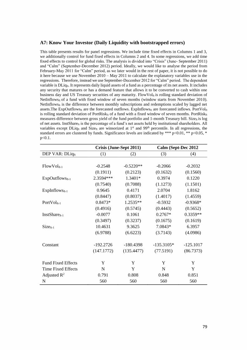
79

A7: Know Your Investor (Daily Liquidity with bootstrapped errors)

This table presents results for panel regressions. We include time fixed effects in Columns 1 and 3,

we additionally control for fund fixed effects in Columns 2 and 4. In some regressions, we add time

fixed effects to control for global risks. The analysis is divided into “Crisis” (June- September 2011)

and “Calm” (September-December 2012) period. Ideally, we would like to analyse the period from

February-May 2011 for “Calm” period, as we later would in the rest of paper, it is not possible to do

it here because we use November 2010 – May 2011 to calculate the explanatory variables use in the

regressions. Therefore, instead we use September-December 2012 for “Calm” period. The dependent

variable is DLiqft. It represents daily liquid assets of a fund as a percentage of its net assets. It includes

any security that matures or has a demand feature that allows it to be converted to cash within one

business day and US Treasury securities of any maturity. FlowVolft is rolling standard deviation of

NetInflowsft of a fund with fixed window of seven months (window starts from November 2010).

NetInflowsft is the difference between monthly subscriptions and redemptions scaled by lagged net

assets.The ExpOutflowsft are the forecasted outflows. ExpInflowsft are forecasted inflows. PortVolft

is rolling standard deviation of PortRiskft of a fund with a fixed window of seven months. PortRiskft

measures difference between gross yield of the fund portfolio and 1-month Treasury bill. Sizeft is log

of net assets. InstShareft is the percentage of a fund’s net assets held by institutional shareholders. All

variables except DLiqft and Sizeft are winsorized at 1st and 99th percentile. In all regressions, the

standard errors are clustered by funds. Significance levels are indicated by *** p<0.01, ** p<0.05, *

p<0.1.

Crisis (June-Sept 2011) Calm (Sept-Dec 2012

DEP VAR: DLiqft (1) (2) (3) (4)

FlowVolft-1 -0.2548 -0.5220** -0.2066 -0.2032

(0.1911) (0.2123) (0.1632) (0.1560)

ExpOutflowsft-1 2.3594*** 1.3401* 0.3974 0.1220

(0.7540) (0.7088) (1.1273) (1.1501)

ExpInflowsft-1 0.9645 0.4171 2.0704 1.8162

(0.8447) (0.8037) (1.4017) (1.4559)

PortVolft-1 0.8473* 1.2535** -0.5932 -0.9368*

(0.4916) (0.5745) (0.4443) (0.5652)

InstShareft-1 -0.0077 0.1061 0.2767* 0.3359**

(0.3497) (0.3237) (0.1675) (0.1619)

Sizeft-1 10.4631 9.3625 7.0843* 6.3957

(6.9788) (6.6223) (3.7143) (4.0986)

Constant -192.2726 -180.4398 -135.3105* -125.1017

(147.1772) (135.4477) (77.5191) (86.7373)

Fund Fixed Effects Y Y Y Y

Time Fixed Effects N Y N Y

Adjusted R2 0.791 0.808 0.848 0.851

N 560 560 560 560

80

A8: Investor Response to Weekly Liquidity (with cash)

The table presents results of panel regressions. We include fund fixed effects in Columns 1 and 3, we

additionally control for time fixed effects in Columns 2 and 4. The analysis is divided into “Calm”

(February-May 2011) and “Crisis” (June- September 2011) period. The dependent variable is

NetInflowsft. NetInflowsft is the difference between monthly subscriptions and redemptions scaled by

lagged net assets. WLiqCft represents weekly liquid assets of a fund as a percentage of its net assets.

It represents weekly liquid assets of a fund as a percentage of its net assets. It includes cash (proxied

by “other assets” reported on N-MFP) any security that matures or has a demand feature that allows

it to be converted to cash within five business days, US government agency securities that mature

within sixty days, and US Treasury securities of any maturity. EZBft is share of a fund’s portfolio

invested in Eurozone banks that were part of 2011 stress tests. We divide the funds into low, medium

and high terciles based on fund portfolio invested in Eurozone banks, Low EZBf and High EZBf

represent funds with lowest and highest EZBft tercile, respectively. InstShareft is the percentage of a

fund’s net assets held by institutional shareholders. WALft is Weighted Average Life calculated as

remaining time to maturity, TTMit of the investment, weighted by its investment weight in fund

portfolio. NetYieldft is the value-weighted average of the 7-day net yields of fund classes as reported

on N-MFP forms. ExRatioft is the expense ratio of funds, calculated as a difference between gross

yield and net yield. GrossYieldis the value-weighted average of issuer yields. NetInflowsft, NetYieldft

and ExRatioft are winsorized at 1st and 99th percentile to remove outliers. In all regressions, the

standard errors are clustered by funds. Significance levels are indicated by *** p<0.01, ** p<0.05, *

p<0.1.

Calm (Feb-May 2011) Crisis (Jun-Sept 2011)

DEP VAR: NetInflowsft (1) (2) (3) (4)

WLiqCft-1 -0.0146 -0.0272 0.0276 0.0378

(0.0661) (0.0681) (0.0698) (0.0681)

EZBft-1 0.2465*** 0.2355** -0.2768* -0.3182*

(0.0898) (0.0964) (0.1457) (0.1654)

Low EZBf * WLiqCft-1 0.0461 0.0496 -0.0272 -0.0174

(0.0472) (0.0461) (0.0240) (0.0222)

High EZBf * WLiqCft-1 -0.0324 -0.0336 -0.0431*** -0.0356**

(0.0278) (0.0272) (0.0149) (0.0157)

WALft-1 0.0822** 0.0784** 0.0367 0.0160

(0.0356) (0.0343) (0.0595) (0.0598)

InstShareft-1 -1.3836*** -1.3897*** -1.2075** -1.0754**

(0.2006) (0.1992) (0.5205) (0.5098)

NetYieldft-1 0.2294 0.2418 -0.2964 0.1070

(0.3069) (0.3169) (0.4108) (0.4295)

ExRatioft-1 0.1679 0.1915 0.3162** 0.5046***

(0.1310) (0.1398) (0.1558) (0.1564)

NetInflowsft-1 -0.1088 -0.1277* 0.0916 0.0587

(0.0735) (0.0727) (0.0823) (0.0761)

Constant 77.7502*** 78.6178*** 77.1016** 62.4855*

(13.6779) (13.7316) (34.4413) (33.7645)

Fund Fixed Effects Y Y Y Y

Time Fixed Effects N Y N Y

Adjusted R2 0.0755 0.0844 0.0889 0.131

N 639 639 654 654

81

A9: Investor Response to Daily Liquidity (with cash)

The table presents results of panel regressions. We include fund fixed effects in Columns 1 and 3, we

additionally control for time fixed effects in Columns 2 and 4. The analysis is divided into “Calm”

(February-May 2011) and “Crisis” (June- September 2011) period. The dependent variable is

NetInflowsft. NetInflowsft is the difference between monthly subscriptions and redemptions scaled by

lagged net assets. DLiqCft represents daily liquid assets of a fund as a percentage of its net assets. It

represents daily liquid assets of a fund as a percentage of its net assets. It includes cash cash (proxied

by “other assets” reported on N-MFP) any security that matures or has a demand feature that allows

it to be converted to cash within one business day and US Treasury securities of any maturity. EZBft

is share of a fund’s portfolio invested in Eurozone banks that were part of 2011 stress tests. We divide

the funds into low, medium and high terciles based on fund portfolio invested in Eurozone banks,

Low EZBf and High EZBf represent funds with lowest and highest EZBft tercile, respectively.

InstShareft is the percentage of a fund’s net assets held by institutional shareholders. WALft is

Weighted Average Life calculated as remaining time to maturity of the investment, weighted by its

investment weight in fund portfolio. NetYieldft is the value-weighted average of the 7-day net yields

of fund classes as reported on N-MFP forms. ExRatioft is the expense ratio of funds, calculated as a

difference between gross yield and net yield. GrossYieldft is the value-weighted average of issuer

yields. NetInflowsft, NetYieldft and ExRatioft are winsorized at 1st and 99th percentile to remove

outliers. In all regressions, the standard errors are clustered by funds. Significance levels are indicated

by *** p<0.01, ** p<0.05, * p<0.1.

Calm (Feb-May 2011) Crisis (Jun-Sept 2011)

DEP VAR: NetInflowsft (1) (2) (3) (4)

DLiqCft-1 -0.0993 -0.0907 0.0695 0.0568

(0.0872) (0.0888) (0.0667) (0.0647)

EZBft-1 0.2485*** 0.2307** -0.2644* -0.3112*

(0.0889) (0.0963) (0.1443) (0.1609)

Low EZBf * DLiqCft-1 0.0714 0.0724 -0.0353 -0.0217

(0.0689) (0.0674) (0.0349) (0.0318)

High EZBf * DLiqCft-1 -0.0588 -0.0579 -0.0615*** -0.0564***

(0.0415) (0.0399) (0.0202) (0.0213)

WALft-1 0.0773** 0.0764** 0.0450 0.0172

(0.0359) (0.0342) (0.0574) (0.0566)

InstShareft-1 -1.3534*** -1.3574*** -1.1931** -1.0595**

(0.2064) (0.2068) (0.5189) (0.5081)

NetYieldft-1 0.2195 0.2272 -0.2583 0.1432

(0.3094) (0.3173) (0.4084) (0.4243)

ExRatioft-1 0.2072 0.2160 0.3339** 0.5226***

(0.1378) (0.1422) (0.1573) (0.1574)

NetInflowsft-1 -0.1112 -0.1265* 0.0938 0.0598

(0.0742) (0.0728) (0.0822) (0.0758)

Constant 77.5022*** 77.7979*** 74.0685** 60.7504*

(14.2345) (14.3789) (34.5257) (33.7875)

Fund Fixed Effects Y Y Y Y

Time Fixed Effects N Y N Y

Adjusted R2 0.0836 0.0901 0.0894 0.132

N 639 639 654 654

82

A10: Wald Tests

The table presents p-values for Wald tests conducted for the sum of coefficients of daily/weekly

liquidity and their interactions with Low and High Eurozone bank share, EZBft tercile reported in

table 3.5 and 3.6 in section 3.3.4, for models with only fund fixed effects and with both fund and time

fixed effects.

Wald test Fund FE only Fund /Time FE

Daily Liquidity

DLiqft-1 + [Low EZBf * DLiqft-1] 0.3777 0.2742

DLiqft-1 + [High EZBf * DLiqft-1] 0.4030 0.2731

Weekly Liquidity

WLiqft-1 + [Low EZBf * WLiqft-1] 0.8682 0.42

WLiqft-1 + [High EZBf * WLiqft-1] 0.9703 0.5194

83

A11: Distribution of Net Inflows in Calm and Crisis

The figure presents the distribution of NetInflowsft. The left-hand panel shows distribution for “Calm”

period (February-May 2011) and the right-hand panel shows distribution for “Crisis” period (June-

September 2011). NetInflowsft is defined as the difference between monthly subscriptions and

redemptions scaled by lagged net assets.

0

.05

.1.1

5

-20 0 20 40 -20 0 20 40

Calm Crisis

De

ns

ity

NetInflows (%)

Distribution of NetInflows in Calm and Crisis

84

A12. Investor Response to Weekly Liquidity (Nested Model)

The table presents results of panel regressions. The dependent variable is NetInflowsft. NetInflowsft is the

difference between monthly subscriptions and redemptions scaled by lagged net assets. CRISISt dummy takes

the value of 0 from February-May 2011 for “Calm” period, and 1 from June- September 2011 for crisis period.

EZBft is share of a fund’s portfolio invested in Eurozone banks that were part of 2011 stress tests. We divide the

funds into low, medium and high terciles based on fund portfolio invested in Eurozone banks, Low EZBft and

High EZBft represent funds with lowest and highest EZBft tercile, respectively. WLiqft-1 represents weekly liquid

assets of a fund as a percentage of its net assets. It includes any security that matures or has a demand feature

that allows it to be converted to cash within five business days, US government agency securities that mature

within sixty days, and US Treasury securities of any maturity. InstShareft is the percentage of a fund’s net assets

held by institutional shareholders. WALft is Weighted Average Life calculated as remaining time to maturity of

the investment, weighted by its investment weight in fund portfolio. NetYieldft -1 is the value-weighted average

of the 7-day net yields of fund classes as reported on N-MFP forms. ExRatioft -1 is the expense ratio of funds,

calculated as a difference between gross yield and net yield. GrossYield is the value-weighted average of issuer

yields. All variables are winsorized at 1st and 99th percentile to remove outliers. In all regressions, the standard

errors are clustered by funds. Significance levels are indicated by *** p<0.01, ** p<0.05, * p<0.1.

DEP VAR: NetInflowsft (1) (2)

EZBft-1 0.1507** 0.142*

(0.0713) (0.0811)

EZBft-1* CRISISt -0.3274*** -0.323**

(0.1253) (0.131)

WLiqft-1 0.0062 -0.00294

(0.0514) (0.0519)

WLiqft-1* CRISISt 0.0148 0.0363

(0.0588) (0.0582)

Low EZBft * WLiqft-1 * CRISISt 0.0067 0.00803

(0.0226) (0.0223)

High EZBft * WLiqft-1 * CRISISt -0.1078** -0.0917**

(0.0478) (0.0429)

NetYieldft-1 0.2481 0.318*

(0.1593) (0.165)

NetYieldft-1* CRISISt -0.3003** -0.226*

(0.1237) (0.123)

ExRatioft-1 -0.0035 0.0138

(0.0672) (0.0726)

ExRatioft-1* CRISISt 0.1497** 0.189***

(0.0709) (0.0708)

WALft-1 -0.0063 -0.00255 (0.0307) (0.0311)

InstShareft-1 -0.6247** -0.603**

(0.2666) (0.275)

NetInflowsft-1 -0.2123*** -0.198***

(0.0397) (0.0399)

CRISISt 1.9064 -1.149

(3.5139) (3.628)

Constant 41.5019** 39.01**

(18.4921) (18.90) Fund Fixed Effects Y Y

Time Fixed Effects N Y

Adj R-squared 0.0950 0.112

Observations 1,293 1,293

85

A13. Investor Response to Daily Liquidity (Nested Model)

The table presents results of panel regressions. The dependent variable is NetInflowsft. NetInflowsft is the

difference between monthly subscriptions and redemptions scaled by lagged net assets. CRISISt dummy takes

the value of 0 from February-May 2011 for “Calm” period, and 1 from June- September 2011 for crisis period.

EZBft is share of a fund’s portfolio invested in Eurozone banks that were part of 2011 stress tests. We divide the

funds into low, medium and high terciles based on fund portfolio invested in Eurozone banks, Low EZBft and

High EZBft represent funds with lowest and highest EZBft tercile, respectively. DLiqft represents daily liquid

assets of a fund as a percentage of its net assets. It includes (1) any security that matures or have a demand feature

that allows it to be converted to cash within one business day (2) US treasury securities of any maturity.

InstShareft is the percentage of a fund’s net assets held by institutional shareholders. WALft is Weighted Average

Life calculated as remaining time to maturity of the investment, weighted by its investment weight in fund

portfolio. NetYieldft -1 is the value-weighted average of the 7-day net yields of fund classes as reported on N-

MFP forms. ExRatioft -1 is the expense ratio of funds, calculated as a difference between gross yield and net yield.

GrossYield is the value-weighted average of issuer yields. All variables are winsorized at 1st and 99th percentile

to remove outliers. In all regressions, the standard errors are clustered by funds. Significance levels are indicated

by *** p<0.01, ** p<0.05, * p<0.1.

DEP VAR: NetInflowsft (1) (2)

EZBft-1 0.1575** 0.145*

(0.0641) (0.0744)

EZBft-1* CRISISt -0.3447*** -0.342***

(0.1017) (0.106)

DLiqft-1 -0.0745 -0.0652

(0.0928) (0.0918)

DLiqft-1* CRISISt 0.1444 0.123

(0.0932) (0.0918)

Low EZBft * DLiqft-1 * CRISISt 0.0232 0.0205

(0.0296) (0.0295)

High EZBft * DLiqft-1 * CRISISt -0.2260*** -0.169**

(0.0679) (0.0660)

NetYieldft-1 0.2653 0.327*

(0.1649) (0.171)

NetYieldft-1* CRISISt -0.2758** -0.209

(0.1265) (0.127)

ExRatioft-1 0.0122 0.0253

(0.0695) (0.0746)

ExRatioft-1* CRISISt 0.1568** 0.198**

(0.0746) (0.0763)

WALft-1 -0.0037 -0.00194 (0.0313) (0.0317)

InstShareft-1 -0.6094** -0.589**

(0.2711) (0.275)

NetInflowsft-1 -0.2063*** -0.193***

(0.0416) (0.0416)

CRISISt 3.0579 0.0410

(2.6254) (2.946)

Constant 39.1510** 37.06*

(18.6064) (18.81)

Fund Fixed Effects Y Y

Time Fixed Effects N Y

Adj R-squared 0.102 0.115

Observations 1,293 1,293

86

Chapter 4 Response of MMF Industry to

the Loss of its Cash-like Nature

4.1 Introduction

In this chapter, we focus on assessing the response of MMFs and their

shareholders to 2016 Amendments. The most notable rules include: (1) the

imposition of liquidity fee and redemption gates, which allows MMFs to charge a

redemption fee or suspend redemptions entirely if the liquidity level of a fund drops

below a certain threshold; (2) Segregation of institutional MMFs from retail MMFs;

(3) and introduction of floating net asset value for institutional MMFs. To the best

of our knowledge, this is the first paper that comprehensively evaluates the impact

of the 2016 Amendments on the MMF industry.

Our contributions to the existing literature are as follows: First, we show that in

the transition period before the new reforms became effective (November 2015 to

October 2016), the migration of total net assets (TNA) from non-government funds

to government funds, also documented in Cipriani et al. (2017), is concentrated

within the sector that has historically proven risky i.e. the prime funds. We do not

observe significant outflows from municipal MMFs.

Second, we investigate the characteristics that influence the decision to convert

to a government fund. This has not been studied before. We document that the

institutional prime funds that belonged to larger fund families were less likely to

convert possibly because they can obtain financial backing from their sponsors (Baba

et al. 2009; McCabe 2010; Kacperczyk and Schnabl 2013; Brady et al. 2012).

87

Specifically, a sponsor can inject liquidity into the fund if a possible breach in the

regulatory liquidity threshold is anticipated. This would help a fund avoid charging

a liquidity fee or suspending redemptions which can adversely impact the reputation

of the sponsor. In addition, we show that funds with higher credit risk were more

likely to convert as they face a higher probability of outflows (Chari and Jagannathan

1988; Jacklin and Bhattacharya 1988; Chernenko and Sunderam 2014). This would

lower the fund’s liquidity reserves and increase the likelihood of eliciting liquidity

fees and redemption gates. Interestingly, we find that retail prime funds with higher

risk tend to stay prime funds possibly because retail investors are significantly less

likely to run during market distress (Gallagher et al. 2015) so such funds are more

likely to engage in yield seeking behaviour. Furthermore, the complete segregation

from institutional investors, now required of retail prime funds, will allow such funds

to reach for yield as their investor base is more stable.

Third, we examine the response of money market funds to liquidity fees and

redemption gates. Previous literature explores the impact of liquidity fees on the run-

behaviour of MMF investors. Cipriani et al. (2014) suggest that liquidity fees make

MMFs more fragile and vulnerable to pre-emptive runs. On the contrary, Lenkey and

Song (2017) find that liquidity fees strengthen informed investors' incentives to

remain invested until maturity. We add new perspective to the debate by providing

empirical evidence of the efforts of institutional MMFs to completely avoid

redemption gates and liquidity fees by hoarding liquidity and by actively adjusting

liquidity in tandem with any increases in credit risk. We contrast this with the period

before the reforms and observe the opposite behaviour. In the pre-reform period,

MMFs decreased their liquidity simultaneously with an increase in the expected loss.

88

Fourth, this is the first paper that observes that after complete segregation of

institutional and retail funds there is greater heterogeneity in portfolio composition

in each type of fund. In addition, we observe distinct fund strategies to guard against

credit risk and heightened institutional fund competition. Gallagher et al. (2015)

suggest that greater concentration of institutional investors will result in increased

demand for liquidity in such funds. We confirm this and show that, as compared to

retail prime MMFs, institutional prime MMFs hold more liquid portfolios. This leads

to a safer asset mix and positions funds to be more resilient to unexpected outflows.

However, this has a negative impact on the institutional funds’ profitability. Further,

Christoffersen (2001) suggests that institutional funds have stronger price

competition than retail funds. We see that, within the MMF industry, greater investor

concentration and the loss of previously attractive money-like features have

strengthened price competition among institutional funds. This occurs as they

endeavour to differentiate themselves by offering higher yields to attract investors.

The rest of the paper proceeds as follows: Section 4.2 provides an overview of

the new regulatory landscape. Section 4.3 describes the data. Section 4.4 presents the

empirical analysis and results. Section 4.5 concludes.

4.2 Regulatory Landscape

MMFs are regulated under rule 2a-7 of the Investment Company Act of 1940,

which restricts funds’ investments to short-term, high-quality debt securities. On July

23, 2014, the SEC announced amendments to rule 2a-7 that governs money market

funds. These amendments have introduced significant structural and operational

changes. The SEC built these changes upon the reforms of March 2010 that dealt

89

with credit, liquidity and interest rate risks. The new reforms provided a two-year

transition period to allow funds to operationally adapt to the new structure whilst

also giving investors time to evaluate their investment options. The compliance date

for the funds was October 14, 2016.

MMFs are primarily divided into three types of funds based on the type of

portfolio securities held. Prime MMFs invest in a variety of corporate debt securities

including certificates of deposit, commercial paper, repurchase agreements and

banker’s acceptances. A government MMF invests at least 99.5 percent (formerly 80

percent) of its total assets in cash, government securities and/or repurchase

agreements that are fully collateralized by cash or government securities. A tax-

exempt (also known as municipal) MMF holds non-taxable municipal securities that

are not taxed by the federal government, nor, in some cases, state and municipalities.

Depending upon risk characteristics, the new rules apply to each MMF sector

differently (Table 4.1). Prime and municipal MMFs have structurally changed and

must comply with several new rules while government MMFs are not significantly

affected by the reforms.

The new rules have introduced investor differentiation and floating NAV

liquidity fee and redemptions gates, enhanced disclosure requirements and enhanced

stress testing. Institutional funds have been the focus of the stricter regulations.

Before October 2016, a management company could offer retail and institutional

share classes for the same portfolio. However, the new reforms have fully segregated

institutional funds from retail funds, which means that for one portfolio, a

90

management company can offer shares to either retail17 shareholders or institutional

shareholders, but not both. Furthermore, institutional prime and municipal/tax-

exempt funds are required to transact at floating NAV. This means that a fund must

use market-based values of their securities to value their portfolio so that the daily

share prices of the funds now fluctuate with the market. This change addresses the

first-mover advantage that institutional investors usually gain at the expense of retail

investors, during a time of crisis. Before the reforms, these funds used the penny

rounding method and a stable NAV of $1.00. Under the new rules, funds must now

use basis point rounding with $1.0000 share price. Government and retail money

market funds continue to use the amortized cost method and/or penny rounding

method of pricing to maintain a stable NAV.

In addition, the prime and municipal funds now have the ability to impose

liquidity fees and redemption gates if certain liquidity thresholds are not met. The

SEC explains that fees and gates are intended to enhance an MMF’s ability to

manage heavy redemptions and make redeeming investors pay their share of the cost

of the liquidity that they receive. Liquidity fee and redemptions gates apply to all

non-government funds, although government funds can also use these tools at their

discretion if they have already announced it in their prospectus. If the fund board

deems it advisable, a money market fund can impose a liquidity fee of up to 2 percent

of redemption amount when a fund’s weekly liquid assets18 fall below 30 percent of

17 A retail money market fund, under SEC 2016 new rules, is defined as a fund that has policies and

procedures which would limit beneficial investors of the fund to natural persons (SEC 2014). 18 Weekly liquid assets include cash, US Treasury securities, government agency securities with

remaining maturities of 60 days or less, and securities that convert into cash within five business days.

91

its total assets. If the fund’s weekly liquid assets fall below 10 percent, then a fund

is required to charge a one percent fee on all redemptions. However, if the fund board

determines that charging a liquidity fee is not in the best interests of the fund or that

a lower or a higher fee (up to 2 percent) is more effective in alleviating the situation,

then it can choose to do so. Alternatively, the fund can suspend redemptions for up

to 10 business days in a 90-day period if a fund’s weekly liquid assets fall below 30

percent, at the discretion of the fund’s board. Any fee or gate must be lifted

automatically after weekly liquid assets rise to or above 30 percent, but it can be

lifted any time before then if the board deems that such a liquidity fee or gate is no

longer in the best interests of the fund. A gate must be lifted within 10 business days.

Additionally, the funds are required to provide daily disclosure on their website

about the fund’s liquidity levels, shareholder inflows and outflows, market-based net

asset values, use of liquidity fee, redemption gates and sponsor support. The funds

must also report additional information relevant to assessing money market fund risk

on the N-MFP2 form. They must also adhere to stronger diversification

requirements, conduct stress tests to maintain at least 10 percent of weekly liquid

assets and ensure minimal principal volatility.

These amendments provide MMFs the tools to deal with heavy redemptions in

times of distress, alleviate first mover advantage, and improve transparency of their

risks. The extent to which the regulators have been successful in achieving this

remains to be seen and is the focus of this paper. We aim to investigate the impact

of the regulation by assessing the response of money market funds and their investors

after the reforms.

92

4.3 Data Description

We create a unique dataset comprising detailed portfolio holdings of US money

market funds which are filed monthly with the SEC monthly over the period from

January 2014 to March 2017. These filings are publicly available from the SEC

EDGAR database. We use several other databases to link the issuers of the MMF

portfolio securities with their parent issuers, countries of domicile and their

annualized expected loss.

The amendments to rule 2a-7 that were introduced in May 2010 require MMFs

to file a monthly report on N-MFP form 19, which includes a detailed schedule of

portfolio holdings of money market funds, starting from November 2010. Since

April 2016, the compliance date for reporting requirements, the reporting of

additional information is required under the new version of the form (N-MFP2).20

Our sample includes information from both versions of the form. We calculate the

variables that were not reported on N-MFP form ourselves, and use the information

reported on the N-MFP2 form for the same variable, after the reforms. For instance,

weekly liquidity of a fund is reported on the N-MFP2 form from May 2016 onwards.

Before this, levels were not required to be reported on the N-MFP form. We calculate

the weekly liquidity21 ourselves before that period.

19This form provides information about fund-level variables like total net assets, gross yield, net yield

and monthly shareholders subscriptions and redemptions. In addition, for each security held, it reports

issuer name, amount of principal, yield, legal maturity date, and the CUSIP number. 20 The additional information includes cash held, daily and weekly liquidity, floating net asset value,

and identifiers of the security issuers and more. 21Weekly liquidity represents weekly liquid assets of a fund as a percentage of its total assets.

93

For our analysis, we aggregate issuer-level variables to the parent level. Then,

we assign a country to the parent. For instance, the securities issued by Bank of the

West, Fortis Funding LLC, Scaldis Capital LLC, Starbird Funding Corporation, as

well the debt issued by BNP Paribas SA are all aggregated under the parent company

BNP Paribas SA. The N-MFP form does not specify the parent company and country

of incorporation of the issuers. We collect this information from a variety of other

datasets22. We use identifiers of the issuers reported on the forms to link them to

other datasets. For the securities for which identifiers are missing, we use the names

of the issuers to merge them with external databases. Using the name of a company

to link different databases can be tricky. The name of a company in one database

often differs from the name used in the other. We employ the “fuzzy string matching”

approach to join the databases. Fuzzy matching allows for non-exact matches to be

joined. To accomplish this, we use the “n-gram” procedure which decomposes the

text string into elements of n characters (grams) using a moving window. The n-gram

algorithm is effective for data with misspellings and large string permutations. One

caveat of fuzzy matching is the “false positive” challenge. The algorithm tends to

match names from one database to another database even when the match is not

completely accurate. To mitigate this concern, we check the matched data line by

line, by hand, to ensure complete accuracy of the matched observations. We are able

22We procure information about global ultimate owners (GUO) of issuers from Wharton Research

Data Services (WRDS), Bloomberg, and Bureau van Dijk’s databases including Amadeus,

Bankscope, Orbis Bank Focus and Osiris. Also, we obtain business card information from the Global

Legal Entity Identifier Foundation (GLEIF). GLEIF maintains key reference information that clearly

identifies legal entities participating in financial transactions. It provides “Level 1” data that has

information on ‘who is who’, and “Level 2” data that describes ‘who owns whom’. After linking the

issuers of MMF securities with Level 1 and Level 2 data, we have some issuers for which the

information is still missing.

94

to obtain information about parents and country of incorporation for the majority of

the issuers.

Next, following Collins and Gallagher (2016) we calculate expected loss to

maturity (ELM) using the default probabilities of issuers obtained from the Risk

Management Institute (RMI) of the National University of Singapore (see appendix

B1). The funds for which less than 75 percent of portfolio securities could be

matched with the default probabilities are removed from the analysis. These

represent only 5 percent of the funds. On average, 92 percent of the total net assets

of the prime funds in our sample are matched with default probabilities. To calculate

the yield spread of money market funds we use US Treasury bill yields which are

collected from the Federal Reserve Economic Data (FRED) database. We have

performed extensive checks and used alternative sources to correct data entry errors.

For instance, the net yield of the funds provided on the N-MFP form is occasionally

incorrectly reported. We obtain the correct values for such funds from Bloomberg.

Our final dataset spans from January 2014 to March 2017. The nature of the

analysis requires the sample to be divided into several periods (Figure 4.1) depending

upon the type of analysis done. We divide the data into before-reform (January 2014

– June 2014) and after-reform (October 2016 – March 2017) to compare fund

portfolio composition of the funds, the fund liquidity management and shareholder

response to the new rules. The before-reform period covers the six months

immediately before the approval of the reforms in July 2014. We select this period

which is more than two years before the after-reform period to make sure it is not

affected by the changes that funds undergo during the transition period to comply

with the new rules. The after-reform period includes the six months from the final

95

compliance month i.e. October 2016 to March 2016. After the announcement of the

reforms on July 23, 2014 there is approximately a two-year window for the funds to

make the required changes by the compliance date. We divide this into pre-transition

and transition periods. Based on graphical evidence (Figure 4.2), the transition period

consists of one year from November 2015 to October 2016 when the fund industry

was making the required structural changes. We select six months before this to be

the pre-transition period (May 2015 to October 2015). This is utilized to test the

characteristics of the funds that decide to change status from prime to government.

4.4 Empirical Analysis

The primary aim of this paper is to study the response of MMFs and their

investors to the 2016 Amendments. The regulation is believed to have fundamentally

altered the basic features that attracted short-term investors to MMFs i.e. intra-day

liquidity and preservation of capital coupled with higher yield. The possibility of

losing these qualities and the uncertainty surrounding the impact of the reforms have

caused massive outflows from the non-government money market funds (Cipriani et

al. 2017). Most of these assets have migrated to government money market funds.

Figure 4.2 and Table 4.2 show that from January 2014 to March 2017, the TNA of

the MMF industry remain constant at around $3 trillion. The TNA within the

different types of MMFs have, however, changed dramatically. The TNA of prime

money market funds have decreased by 67 percent from $1,794 billion to $599

billion. The share of prime fund TNA has dropped by 39 percent down to only 20

percent of industry TNA in March 2017. Municipal funds have dropped by 52

percent to $135 billion. Government funds have increased dramatically to $1,226

96

billion, a 127 percent rise in March 2017. The market share of the government funds

has increased by 43 percent to 75 percent of the industry TNA. This reduction in the

TNA of prime funds and increase in government funds shows investors’ preference

for liquidity and preservation of capital. Figure 4.3 shows the number of each type

of fund from January 2014 to March 2017. Prime funds and municipal funds have

decreased while the number of government funds have increased significantly. This

indicates that the migration of TNA from non-government MMFs is not only because

of investors moving their money from prime funds to the existing government funds

but also because of the funds’ decision to convert to government funds. In section

4.4.1, we empirically test the statistical significance of the changes in the TNA of

the funds.

4.4.1 Changes in Total Net Assets of MMFs

The 2016 Amendments to rule 2a-7 impose liquidity fee and redemption gates on

all prime/municipal funds and floating NAV on institutional prime and municipal

funds. However, these rules do not apply to government funds. Consequently, it

appears that the non-government funds have transferred a massive amount of assets

to government funds to evade the new rules which are presumed to thwart the ability

of investors to make same day withdrawals or do so at a cost. Prime MMFs have

been popular for providing same-day liquidity, preservation of capital, and higher

yields. The possibility of losing these features has caused the industry to migrate

from prime and municipal funds to government funds. An increase in the number of

government funds (Figure 4.3) indicates that the funds have converted to this

category. In this scenario, we expect that the funds would be converted within the

97

same family23. Cipriani et al. (2017) also find that most of this transfer is

concentrated within the same fund family. To account for this, we conduct the

analysis at a fund family level.

We investigate the changes in the TNA of the funds after the 2016 Amendments

using the following panel fixed effects model:

Yfft =αff + β1 Reformt + µt + εfft eq. (1)

where Yfft represents a fund family’s TNA calculated separately for each category of

fund and the shareholder type it serves. For instance, we aggregate the TNA of all

retail prime funds of a fund family separately from all institutional prime funds of

the family and repeat the process for municipal and government funds of the family

aggregating the TNA by either retail or institutional fund. So, Yfft represents six

variables: NAPrimeIfft and NAPrimeRfft which are calculated as a sum of TNA of a

fund family “ff” invested in all institutional prime funds and all retail prime fund,

respectively; NAMuniIfft, NAMuniRfft, NAGovtIfft, NAGovtRfft calculated as a sum

of TNA of a fund family “ff” invested in all institutional municipal funds, all retail

municipal funds, all institutional government funds and all retail government funds,

respectively. Before reforms, a fund with an institutional share greater than 99

percent is identified as an institutional fund, otherwise it is a retail fund. Institutional

share is the share of a fund’s ownership in institutional share classes. Following

Chernenko and Sundaram (2014), a share class is considered institutional if it has a

minimum investment of $ 1,000,000 has “institutional” in the name of the class.

23A fund family is an investment company which invests in one or more money market funds. A fund

family is identified by the CIK number of a fund manager as reported on the N-MFP form. Table 4.3

shows that, in our sample, there is a total of 282 fund families before reforms and 226 families after

reforms.

98

After reforms, a fund is identified as retail or institutional on the N-MFP2 form, so

we utilize that information. αff represents fund family fixed effects and enables with

control for possible endogeneity that might result from a correlation of unobserved

fund family-specific attributes with the explanatory variables. We add time fixed

effects, µt, to control for global risks. Reformt takes the value of zero before reforms

(January 2014 – June 2014), which is the six-month period immediately before the

reforms were introduced. It takes the value of one from October 2016 to March 2017,

a period that comprises the six months after the reforms became effective in October

2016. The industry becomes stable after the compliance date which makes it

unnecessary to go beyond this six-month period. For consistency, both before- and

after-reform periods are six months long. εfft is the error term clustered at the fund

family level.

Table 4.4 presents the regression results. Columns (1-4) show that β1 for both

retail and institutional prime/municipal funds is negative and significant indicating

that the TNA in these two types of funds has decreased significantly. Institutional

prime and municipal funds’ decrease in TNA indicates the desire to avoid the

requirements such as redemption gates, liquidity fee and the imposition of floating

NAV. A liquidity fee is a fee charged against the redemption amount and retained

by the fund. It is intended to deter investors from withdrawing shares during stressful

periods to avoid sudden heavy outflows, boost liquidity levels by injecting cash

withheld from redemptions, and remove the first mover advantage. It results in a loss

of capital and lower investor return. A redemption gate is a temporary suspension of

the redemption of a fund’s shares. It leads to a loss of liquidity and access to money.

99

While redemption gates and liquidity fees are mutually exclusive, the imposition of

a liquidity fee can be followed by the imposition of redemption gates.

The decrease in TNA of institutional funds is consistent with the fact that

institutional investors are active and tend to withdraw from funds if there is a risk of

losing unhindered access to money and of loss of capital (Jacklin and Bhattacharya

1988; Chordia 1996; Greene et al. 2007). Anecdotal evidence suggests that this

decrease has partially occurred because of the decision of funds to convert

themselves into government funds without investors having to withdraw the money.

This decision is because the institutional funds are serving a more active and volatile

shareholder base and are expected to be more prone to runs during distress (Wermers

2011; Schmidt et al. 2016). Therefore, they will have a higher probability of

imposing liquidity fees or redemption gates. This could taint the reputation of the

fund family and fund sponsors. Unfortunately, we are not able to separate the impact

of redemption gates and liquidity fees from the impact of floating NAV in

institutional funds and other confounding effects. However, it can be observed

clearly from the decrease in TNA of retail prime/municipal funds because these

funds are not subject to floating NAV. Therefore, the reduction in TNA of retail

funds could be interpreted as the response of investors to redemption gates and

liquidity fees. However, one must keep in mind that other changes in financial

markets such as bank reforms (Basel III) may have indirectly influenced the decision

of investors to some extent. Retail investors have historically been inactive investors.

Then, one would expect these funds to have less reason to worry about imposing a

redemption gate or liquidity fee, and therefore have lower reputational risk. The

reason for the decrease is possibly because the redemption gates/liquidity fees have

100

changed the nature of money market funds. During calm periods, these funds can be

treated as money-like, but in distress periods, the investors either cannot redeem, if

redemptions are suspended, or can withdraw at will, albeit at a possible loss of

principal if a liquidity fee is imposed.

Columns (5-6) show that both retail and institutional government funds have

increased TNA, post reform. Government money market funds may, but are not

required to, use liquidity fees and redemption gates. In addition, these funds are not

required to float NAV and can continue to operate at stable NAV. These funds

maintain the pre-reform nature of money market funds and hence seem to be more

in-demand after the reforms. So, the transfer has occurred because of i) the investors’

decision to move to government funds and ii) the funds’ decision to change their type

and portfolio composition to become government funds. Next, we empirically test

whether the increase in the TNA of government funds is in fact due to migration of

TNA from prime and municipal funds.

4.4.2 Migration of Total Net Assets of MMFs to Government Funds

In this section, we investigate the flows between different types of money market

funds. We conduct the study using the changes in total net assets to capture both i)

the withdrawals made by shareholders ii) the instances where a fund reclassifies itself

from prime/municipal to government. Conversely, if we use redemptions and

subscriptions we will miss out the transfer of TNA of a fund to government funds

that was done by changing the category of funds through broker-dealers without

requiring investors to withdraw their money. To capture this, the analysis is carried

out at the fund family level. An increase in a fund family’s government TNA and a

101

decrease in prime and municipal net assets represents a fund reclassification. If the

changes in the TNA of different types of MMFs is because of the reforms, then we

would expect the migration of money to remain within the same fund family. This

analysis is similar to Cipriani et al. (2017), but we extend the analysis by examining

the migration of money from retail/institutional prime and municipal funds

separately to discover which funds respond more sharply.

We run panel regressions including time and fund family fixed effects. Time-

fixed effects are included to control for global risks. Fund family fixed effects are

added to observe the within-fund family variation in the total net assets. We run the

following model over the transition period from November 2015 to October 2016,

the time when the industry was adjusting to comply with new regulations,

∆NAGovtfft =αff + β1 ∆NAPrimeIfft + β2 ∆NAPrimeIfft-1 + β3 ∆NAPrimeRfft +

β4 ∆NAPrimeRfft-1 + β5 ∆NAMuniIfft +β6 ∆NAMuniIfft-1 + β7 ∆NAMuniRfft +

β8 ∆NAMuniRfft-1 + µt + εfft eq. (2)

The dependent variable, ∆NAGovtfft, is the monthly change in a fund family’s

TNA held in government funds. We calculate TNA of each type of fund held by each

family separately to clearly identify which funds convert to government funds.

∆NAPrimeIfft and ∆NAPrimeRfft represent the first differences of a fund family’s

TNA invested in institutional prime and retail prime funds, respectively.

∆NAMuniIfft, and ∆NAMuniRfft, represent the first differences of a fund family’s

TNA invested in institutional municipal funds and retail municipal funds,

respectively. We control for lagged changes in all variables to account for delayed

transfers.

102

Table 4.5 displays the results for changes in TNA of government funds of a fund

family in relation to changes in TNA of its prime and municipal funds. Column 1

shows that contemporaneous changes in TNA of institutional prime funds,

∆NAPrimeIfft, is highly statistically significant and is negatively related to changes

in government TNA of the fund family. This indicates that a fund family’s decrease

in institutional prime TNA had led to an increase in government TNA. This shows

that the reforms have led to the migration of funds from prime to government fund.

The coefficient of ∆NAPrimeIfft is -0.78 which is very high showing that most of the

increase in government funds is driven by a decrease in a family’s institutional prime

funds. Additionally, we control for its lagged changes, ∆NAPrimeIfft-1, to capture the

variation in case there is a delay in transferring assets from one fund to another, i.e.

the transfer is not contemporaneous. The coefficient is negative and significant,

hence reinforcing the previous results. Next, the changes in retail prime total net

assets, ∆NAPrimeRfft show that retail funds are also transferring TNA from prime to

government. The coefficient is -0.12 which is very small as compared to institutional

prime funds, suggesting lower variation in ∆NAPrimeRfft because of retail funds.

The sum of the coefficients, β1 + β2 + β3 is equal to -1.01, indicating almost one-to-one

migration of assets from prime funds to government funds. Cipriani et al. (2017) find

a similar relationship.

On the other hand, coefficients of municipal funds are insignificant. This is

because municipal funds are inherently different from prime and government funds.

First, these are not risky like prime funds because they only invest in municipal

securities issued by local or state governments. Second, it is possibly harder for such

funds to easily transfer to government funds because these must change status from

103

tax-exempt to taxable funds, as well as change their entire portfolio to government

securities. Third, the shareholder base of these funds has not proven to be a volatile

one, so there does not seem to be much incentive to change to a different type of

fund. The municipal funds seem to be safer than government funds as evidenced

from the fact that the investors withdrew heavily from government funds during the

US debt ceiling impasse of 2011. The municipal funds have never been in trouble,

historically. Cipriani et al. (2017) find that non-government funds migrate their TNA

to government funds, but we clarify that such migration is statistically significant

only for prime money market funds.

It might be the case that a fund family’s increase (decrease) in one type of fund

always results in a decrease (increase) in the other type. Therefore, we run a placebo

regression, before reforms from January 2014 – June 2014.24 This is about two years

before the SEC regulation compliance deadline and therefore is not influenced by

the transition period. Column 2 shows that during this period, the slope coefficient

on prime institutional funds’ contemporaneous, changes, ∆NAPrimeIff, and lagged

changes, ∆NAPrimeIfft-1, is positive and highly significant. This indicates that,

usually, an increase in government TNA is accompanied by an increase in the TNA

of institutional prime funds of the same family. Therefore, it is only in the year before

the compliance date that investors moved their assets from prime to government

funds within the same family, which indicates that such migration is driven by the

reforms. The analysis indicates that municipal funds have not changed dramatically

after the reforms, so the rest of our paper focuses only on prime money market funds.

24 A regression for a one-year sample also produces similar results.

104

4.4.3 Factors that Influenced Decision of Prime MMFs to Change

Category

In this section, we attempt to understand the characteristics of the prime MMFs

that predict a change to government funds, which has not been analysed before. We

estimate a pooled probit model over the pre-transition period, from May 2015 –

October 2015, the six months just before the funds started to make changes to comply

with the new rules. We choose six months to be consistent with the choice of other

periods in the paper.25 We estimate the following regression separately for

institutional and retail prime funds:

Changef = α + β1 NoOfFundsft + β2 Sizeft + β3 ELMft + β4 FlowVolft +

β5 ExRatioft + β6 WLiqft + εft eq. (3)

where Changef is a dummy variable which takes the value of 1 if a fund, “f” exits

prime fund by the compliance deadline of October 2016, otherwise 0. NoOfFundsft

represents the size of a fund’s family as measured by the number of MMFs a fund

family manages. Sizeft is the log of total net assets of a fund. ELMft is the expected

loss at maturity which represents the credit risk of a fund (see appendix B1 for

calculations). WLiqft is the weekly liquidity which represents a fund’s weekly liquid

assets of the fund as a percentage of its total assets. FlowVolft is the flow volatility,

calculated as rolling standard deviation of a fund’s NetInflowsft over a fixed window

of the past six months, where NetInflowsft are calculated as the difference between

subscriptions and redemptions. ExRatioft is the expense ratio of a fund, which

represents the difference between gross yield (a fund’s portfolio yield) and net yield

25We conduct a robustness test on the period from July 2014 to October 2015 which includes the

whole stretch of time from the approval of 2016 amendments to rule 2a-7 in July 2014 to October

2015 which is a month before transition period starting in November 2015. We find that the results

are robust (see appendix B3).

105

(yield paid to a fund’s investor). εft is the error term. We cluster standard errors by

fund. We run the regression separately for institutional and retail funds. Institutional

prime funds are subject to stricter requirements than retail prime funds, so we expect

them to behave differently than retail funds.

Table 4.6 summarizes the results.26 Columns 1 and 2 represent the coefficients

and marginal effects of the probit model in eq. (3), for institutional prime funds,

respectively. In column 2, NoOfFundsft is negative and highly significant.

Institutional funds that belong to bigger fund families are less likely to change to

government funds or quit. Such funds, when in distress, can acquire financial

support from their sponsor. McCabe (2010) shows that sponsors’ support slowed

the investor withdrawals in 2007. Brady et al. (2012) find that at least 21 prime funds

received support from their sponsors to avoid “breaking the buck” during the global

financial crisis. A fund sponsor even though not contractually required to do so, often

chooses to support an MMF to avoid reputational risk which can have a negative

impact on the sponsor’s other businesses. Post reforms, the institutional prime funds

became obligated to use floating NAV so breaking the buck is no longer a concern.

However, they must impose liquidity fees and redemption gates when liquidity levels

drop below a certain threshold. However, a fund can avoid liquidity fees and

redemption gates by obtaining financial support from its sponsors to increase

liquidity levels.

The marginal effects of Sizeft are negative and significant indicating that the

bigger funds are less likely to change their category. Judging from the fact that bigger

26The results are robust to a specification including time-fixed effects (see appendix B2).

106

funds are managing more net assets, these funds have demonstrably higher capability

to attract and retain investors. Therefore, they are possibly more confident in their

ability to continue to do so in the post-reform era. Other reasons could be that bigger

funds are slower to change and are better at managing relationships with their

shareholders which would allow them to predict outflows more accurately and hence

be able to manage their liquidity more effectively. Next, the coefficient of ELMft

which is a fund’s expected loss at maturity, a measure of portfolio credit risk, is

positive and significant. Institutional prime funds with higher credit risk are more

likely to change to government funds because funds with higher credit risk have a

greater possibility to undergo distress (Chari and Jagannathan 1988; Jacklin and

Bhattacharya 1988; Chernenko and Sunderam 2014), which could lead to higher

outflows and lower liquidity with an increased likelihood of eliciting liquidity fees

and redemption gates. Higher credit risk would also give rise to more volatility in a

fund’s floating NAV which could lead to investor withdrawals because of potential

loss in the principal invested. Therefore, converting to a government fund would lead

to a more stable fund with no requirement for floating NAV, redemption gates or

liquidity fees. The marginal effects of the expense ratio, ExRatioft, weekly liquidity

WLiqft, and flow volatility, FlowVolft, are insignificant, indicating that these do not

play a part in a fund’s decision to exit prime funds.

Columns 3 and 4 represent the coefficients and marginal effects for retail prime

funds. In Column 4, the coefficient of NoOfFundsft is insignificant indicating that,

unlike with institutional funds, the size of a fund family is not a determining factor

in the decision of a retail fund to change category. The coefficient on Sizeft shows

that the bigger retail funds do not change their category in response to the reforms.

107

This is possibly because such funds have demonstrably higher capacity to attract

inflows, retain investors and have possibly better relationships with shareholders

with greater ability to manage outflows and hence liquidity levels. Interestingly, the

funds with higher ELMft, tend to stay prime funds. This could be because retail funds,

unlike institutional funds, do not have a very volatile shareholder base. In previous

episodes of crisis, retail investors remained significantly less likely to withdraw

during market stress (Gallagher et al. 2015). This is because retail investors do not

usually have resources to assess the quality of a fund’s portfolio. Therefore, retail

funds do not have the incentive to keep the credit risk of their portfolio low because

they are managing slow money. Moreover, the new reforms prohibit institutional

investors from investing in retail funds which means that the market discipline

enforced by the institutional investors before reforms has been eliminated. Therefore,

retail funds can invest in riskier assets without potentially adverse consequences. The

marginal effects of FlowVolft is positive and significant. Retail funds with higher

flow volatility are more likely to change to government funds because higher flow

volatility results in unpredictability of inflows/outflows and hence more volatility in

liquidity levels. The marginal effects of ExRatioft and WLiqft, are insignificant.

4.4.4 Changes in Retail vs Institutional Prime Funds

The requirement of redemption gates and liquidity fees means that after the

reforms if a fund is subject to heavy withdrawals and its liquidity goes below a

certain level it can restrict the redemptions for a maximum period of 10 days or

charge a fee on redemptions. Several funds advertise that they do not plan to impose

gates nor charge liquidity fees. Therefore, we expect funds to position themselves so

108

that they can avoid scenarios where they might be forced to restrict redemptions. We

document changes in retail and institutional prime funds’ portfolio composition after

the reforms. This is the first paper to engage in such analysis.

Table 4.7 reports the averages and statistical significance of the variables that

describe the composition of MMF portfolios before reforms (BR) from January 2014

to June 2014 and after reforms (AR) from October 2016 to March 2017. “Diff”

represents the difference between “AR” and “BR”. Column 3 shows the differences

between the averages of the reported variables before and after reforms. The average

size of an institutional prime fund, NetAssetsft has not changed significantly.27 The

funds have increased their weekly liquidity, WLiqft to 67 percent on average, to

ensure that they do not the breach 30 percent threshold that could lead to imposition

of redemption gates or liquidity fees. In addition, they have lowered weighted

average life, WALft which leads to lower average maturity and a more liquid

portfolio. The assets with longer maturities have largely decreased. On average, the

expected loss of a fund, ELMft has increased by 2.85 bp indicating that funds are

taking more risk. Post-reform, the increase in the regulatory burden has increased the

cost of operations. The new rules have stripped funds of features such as preservation

of capital and money-like liquidity, making MMFs less attractive than before. To

attract investors a fund must earn higher yield (Sirri and Tufano 1998; Koppenhaver

and Sapp 2005), to cover the increased expenses and pay a competitive yield to

shareholders. To earn higher yield, it must invest in riskier securities (Kacperczyk

27The total net assets of MMFs are known to be positively skewed, which would lead to a biased

mean. As a robustness test, we calculate the significance of the differences between the median net

assets, which is also insignificant (see appendix B4).

109

and Schnabl 2013). Next, Spreadft indicates that institutional funds have, in fact,

increased the portfolio gross yield net of the average government fund gross yield.

(NetYieldft - GovtNY̅̅ ̅̅ ̅̅ ̅̅ ̅̅ ft) indicates that after accounting for the increases in the treasury

yield during the period under analysis, the funds are paying a higher yield after the

reforms (+12.26 bp). Also, the funds are charging higher management fees to meet

the added cost of the new regulations, as seen from the increase in the expense ratios,

ExRatioft.

Column 6 displays the differences in the averages of the variables for retail funds

before and after the reforms. The retail funds have the similar response in sign and

significance for all the variables, but the magnitude of the average values differ in

most cases. Columns 7 and 8 compare these differences in institutional and retail

funds before and after reforms. After reforms, institutional funds hold more WLiqft

(+15.55%) than retail funds which is five times more than the difference before

reforms. These funds also have lower WALft (-15.96 %) than their retail

counterparts. There was no significant difference in WALft of the funds earlier. The

difference in the liquidity of these funds is understandable as these have different

liquidity management goals because of structural differences in the post-reform era.

Institutional funds serve a more volatile shareholder base and are subject to the

floating NAV requirement. They must strive to keep the NAV stable which translates

into maintaining lower risk and a more liquid portfolio. Because they manage hot

money, they also need higher liquidity to withstand heavy redemption pressure.

Figure 4.4 shows the average proportion of the total portfolio securities invested in

each maturity range for institutional and retail funds. The institutional funds seem to

110

have changed WLiqft and WALft by investing a higher proportion of assets in very

short-term securities that mature within 5 days, and disinvesting in longer maturity

securities. Conversely, retail funds decrease their short-term investments and invest

more in securities with maturities >180 days (Figure 4.4) which explains the

difference in liquidity and WALft. The expected loss, ELMft is not significantly

different for both types of funds. However, Figures 4.5 and 4.6 show that the source

of the ELMft for both types of funds is different. Figure 4.5 shows that the ELMft of

institutional MMFs has increased from all regions including Asia and Pacific,

Europe, North America and Other. This could be interpreted as a more cautious risk

management strategy where the funds have diversified the credit risk. Institutional

MMFs (Figure 4.6) have very slightly increased their investments in Europe, but they

keep investing roughly the same proportion of their assets in each region as compared

to before the reforms. Retail MMFs have decreased the total proportion of securities

invested in Asia and Pacific and Europe and increased their investment in North

America.

Institutional funds are earning a lower yield spread, Spreadft, (-8.56 bp) than retail

funds, which is four times lower than the difference before reforms. However, they

still pay a higher net yield to their investors, NetYieldft - GovtNYt̅̅ ̅̅ ̅̅ ̅̅ ̅̅ ̅. These funds are

able to pay higher yields while earning lower Spreadft by charging lower fees than

retail funds do. The expense ratio of institutional funds (-19.54 bp) is very low as

compared to that of retail funds. Christoffersen (2001) demonstrates that 79 percent

of institutional MMFs waive fees whereas only 55 percent of retail funds do so,

implying that institutional funds have stronger price competition than retail funds.

111

The expense ratio of institutional funds is approximately seven times lower than the

difference before reforms. Furthermore, retail funds have less incentive to charge

lower fees because retail investors are less sensitive to fund performance and tend to

remain invested in funds that charge higher fees (Christoffersen and Musto 2002). It

seems that higher investor concentration, stricter rules and loss of the attractive

features of MMFs have strengthened competition in institutional funds. However,

other regulations such as those in Basel III and the Dodd-Frank Act might be

affecting the analysed measures as well. Unfortunately, it is not possible to separate

the impact of these regulations from the impact of SEC regulation.

In summary, we find that the institutional funds have changed their portfolio

composition dramatically in the port-reform era. In addition to the structural changes

imposed by the regulations, the two types of funds have become very different in

their liquidity positions, maturity structure and competitiveness. Institutional funds

are foregoing more management fee to pay higher yields to their investors and

maintain their competitiveness.

4.4.5 Liquidity Management at MMFs After 2016 Amendments

In addition to the minimum regulations, in chapter 3, we show that portfolio

composition and shareholder behaviour determine the levels of liquidity a fund

holds. They document that higher flow volatility, expected outflows and riskier

portfolios maintain higher liquidity suggesting that the funds keep a safety cushion

if they have a higher chance of withdrawals. We extend the analysis by further

investigating the relationship between contemporaneous changes in liquidity and

credit risk of a fund. MMFs have several reasons to manage the weekly liquidity of

112

their portfolio actively. First, they must have a regulatory minimum of 30 percent of

their total assets in weekly liquid assets. Second, new rules require funds to charge

liquidity fees or suspend redemptions if the weekly liquid assets fall below this

regulatory minimum. Third, if it has higher risk it must maintain a safety cushion to

meet redemptions comfortably because during market distress, runs are more severe

for MMFs that have lower portfolio liquidity (Wermers 2011). We thus test whether

the funds are managing their liquidity according to their risk profile. The empirical

model is specified as follows:

∆WLiqft = αf + β1 ∆ELMft + β2 ELMft-1 + β3 ∆NetInflowsft +

β4 NetInflowsft-1 + εft eq. (4)

where ∆WLiqft is monthly change in weekly liquidity of fund “f”. αf represents fund

fixed effects. We include the change in the expected loss of a portfolio, ∆ELMft. This

is the main regressor of interest. An increase in credit risk raises the likelihood of

default, which could lead to heavy outflows and hence a higher need for liquid assets.

Given that funds base their liquidity levels on the portfolio composition and

redemption behaviour of their investors, we expect any increase in credit risk to be

accompanied by a contemporaneous growth in liquidity, which should result in a

positive β1. We include ELMft-1 to account for delayed adjustments in fund liquidity.

A higher lagged credit risk should encourage funds to hold more liquid holdings.

Therefore, we expect a positive β2. We add contemporaneous changes in net inflows,

∆NetInflowsft in the regression to capture variation in liquidity caused by changes in

funds’ net subscriptions. NetInflowsft is calculated as the difference between

subscriptions and redemptions. Positive net inflows inject cash in the fund which

113

would result in higher liquidity, while negative net inflows decrease liquidity

because funds must sell their liquid assets to meet redemptions. We add lagged net

inflows, NetInflowsft-1 as a control variable to capture possible delays in rebalancing

the portfolio to achieve the desired liquidity levels.

One caveat of including ∆ELMft and ∆NetInflowsft as regressors is that there

might be reverse causality between changes in liquidity, expected loss and net

inflows. To address this problem, we instrument these variables with their predicted

values.28 The analysis is conducted separately for institutional and retail funds. We

further divide the sample into before-reform and after-reform to observe any changes

in fund behaviour after the introduction of the new rules.

Table 4.8 presents the results of eq. (4). Column 1 shows regression results for

institutional prime funds before reforms. The coefficient of ∆ELMft is negative and

significant indicating that an increase in expected loss results in a decrease of

portfolio liquidity. In other words, a fund’s liquidity decreases contemporaneously

as credit risk increases. This is possibly because a fund invests a large proportion of

its assets in longer maturity instruments to increase the expected loss, which leads to

a lower proportion of assets invested in short-term liquid assets. It is well

documented that the funds increase their credit risk to earn higher yields

(Koppenhaver 1999; Chernenko and Sunderam 2014) to attract more inflows. The

28For NetInflowsft, we estimate the following regression: ∆NetInflowsf,t = α +

∑ β1 ∆NetInflowsf,t−nN=5n=1 + ∆NetYieldf,t−1 + εf,t where n is the number of lags. To obtain fitted

values for ∆ELMft the following model is estimated: ∆ELMf,t = α + ∑ β1 ∆ELMf,t−nN=5n=1 +

∆WALf,t−1 + εf,t. Using fitted values in eq. (4) helps address endogeneity concerns but could lead

to biased coefficients. We conduct a robustness test by using bootstrapped standard errors and find

that the results are robust (see appendix B5). Further, we employ a different lag specification to

calculate the fitted values of the variables and show that the results are robust (see appendix B6).

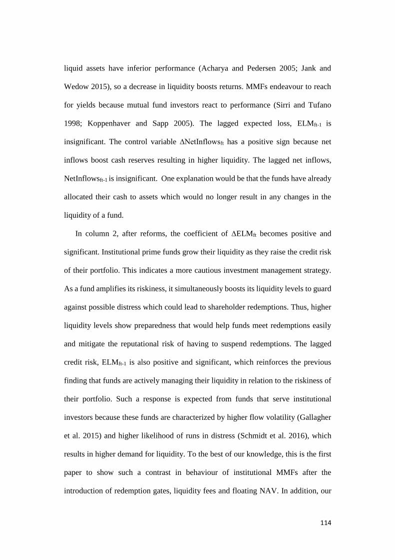
114

liquid assets have inferior performance (Acharya and Pedersen 2005; Jank and

Wedow 2015), so a decrease in liquidity boosts returns. MMFs endeavour to reach

for yields because mutual fund investors react to performance (Sirri and Tufano

1998; Koppenhaver and Sapp 2005). The lagged expected loss, ELMft-1 is

insignificant. The control variable ∆NetInflowsft has a positive sign because net

inflows boost cash reserves resulting in higher liquidity. The lagged net inflows,

NetInflowsft-1 is insignificant. One explanation would be that the funds have already

allocated their cash to assets which would no longer result in any changes in the

liquidity of a fund.

In column 2, after reforms, the coefficient of ∆ELMft becomes positive and

significant. Institutional prime funds grow their liquidity as they raise the credit risk

of their portfolio. This indicates a more cautious investment management strategy.

As a fund amplifies its riskiness, it simultaneously boosts its liquidity levels to guard

against possible distress which could lead to shareholder redemptions. Thus, higher

liquidity levels show preparedness that would help funds meet redemptions easily

and mitigate the reputational risk of having to suspend redemptions. The lagged

credit risk, ELMft-1 is also positive and significant, which reinforces the previous

finding that funds are actively managing their liquidity in relation to the riskiness of

their portfolio. Such a response is expected from funds that serve institutional

investors because these funds are characterized by higher flow volatility (Gallagher

et al. 2015) and higher likelihood of runs in distress (Schmidt et al. 2016), which

results in higher demand for liquidity. To the best of our knowledge, this is the first

paper to show such a contrast in behaviour of institutional MMFs after the

introduction of redemption gates, liquidity fees and floating NAV. In addition, our

115

results confirm the concern of Gallagher et al. (2015) that greater concentration of

institutional investors will result in increased demand for liquidity in such funds.

Column 3 displays the results for eq. (4) for retail prime funds, before reforms.

As the expected loss increases, retail funds increase their portfolio liquidity which is

a cautious investment strategy to maintain safe liquidity levels. All control variables

are insignificant. In column 4, after reforms, the contemporaneous change in

expected loss, ∆ELMft has an insignificant impact on the liquidity levels of the fund

which is interesting. Unlike institutional funds, the retail funds do not seem to

increase liquidity actively post reforms. This is possibly because the market

discipline enforced by institutional shareholders is eliminated, because after reforms

retail funds are only offered to “natural persons” who rebalance their portfolio less

frequently. The control variables ∆NetInflowsft and NetInflowsft-1 are insignificant.

In summary, in the post-reform period, institutional prime funds have become

more active in their management of credit risk. They adjust their liquidity levels

upwards simultaneously with any increases in their credit risk resulting in increased

safety to control for possible redemption pressure. On the other hand, retail funds

have become more relaxed in their liquidity management.

4.4.6 Shareholders’ Response to New Rules

The new rules have consequences for investors in money market funds. They

could lose access to capital if redemption gates are applied or incur costs if liquidity

fees are imposed. So, post reform the institutional investors must be more cautious

of the credit risk and liquidity levels of the portfolio investments in the MMFs.

Historically, heavy redemption pressure occurs when the fund’s securities become

116

riskier.29 Many fund families have taken actions to limit the possibility of a

redemption trigger or avoid it altogether by converting their funds into government

money market funds, which have no such requirement.

In this section, we examine the response of each type of shareholder after

reforms. We estimate the following panel fixed effects regression:

NetInflowsft = αf + β1 ∆ELMft + β2 ELMft-1 + β3 ∆WLiqft + β4 WLiqft- +

β5 Cft-1 + εft eq. (5)

where the dependent variable NetInflowsft is calculated as a difference between

monthly subscription and redemptions as a percentage of the lagged total net assets

of fund “f”. αf represents fund fixed effects. ∆ELMft is the predicted change in the

expected loss at maturity of a fund’s portfolio and is defined as before. ∆WLiqft is

the predicted change in weekly liquidity. ELMft-1 and WLiqft-1 are lagged expected

loss and weekly liquidity, respectively. We include but do not show the following

control variables represented by Cft-1 matrix that could influence the behaviour of a

fund’s shareholders: NetYieldft-1, which is the yield earned by funds’ shareholders,

calculated as the value-weighted average of the 7-day net yields of the fund share

classes as reported on N-MFP form; Sizeft, the log of total net assets of a fund;

ExRatioft, the expense ratio of a fund calculated as the difference between the gross

yield and the net yield of a fund. Standard errors are clustered by fund.

29For instance, the Lehman Brothers default in September 2008 triggered industry wide redemptions

and the Reserve Primary funds “broke the buck”. In June 2011, during the sovereign debt crisis,

investors withdrew heavily from the MMFs with high Eurozone bank exposures because such banks

were expected to default due to their large holdings of sovereign debt. Most of these withdrawals

were made by institutional investors.

117

Table 4.9 presents the results.30 Column 1 shows the results for institutional

prime funds before reforms. All the main explanatory variables are insignificant.

This is plausible because MMFs hold high quality short-term debt instruments and

are governed by rule 2a-7 which ensures stable NAV and low-risk portfolios. This

enabled MMFs to offer attractive features such as preserving capital, providing

intraday liquidity coupled with higher yields before reform. With such features,

investors were not very concerned about the portfolio composition before reforms

during calm periods. This has changed after reforms. In column 2, we examine the

response of investors to credit risk and liquidity of a fund portfolio, after reforms.

We find that investors respond negatively to higher credit risk portfolios. This is

expected because post-reform, in the event of distress, investors can lose access to

capital if redemption gates are applied or redeem their money at a cost if a fund

decides to charge a liquidity fee. Furthermore, we expect institutional investors to

be watchful of the changing risk of a fund. We test this by using the contemporaneous

changes in the expected loss of a fund as an additional regressor, ∆ELMft. The

coefficient is negative and highly significant. So, institutional investors tend to

disinvest from funds with higher credit risk. The contemporaneous changes of net

inflows with changes in expected losses points to the cautious attitude of institutional

investors to the risk of a portfolio. This prudent behaviour of institutional investors

is corroborated by Gallagher et al. (2015) who find that after controlling for net

yields, institutional investors react negatively to increases in gross yield which

30The results presented in table are robust to regression bias (see appendix B7), persistence of net

inflows (we run a dynamic regression) (see appendix B8) and different specification of

contemporaneous variables (see appendix B9).

118

represents risk. The weekly liquidity of a fund has become a critical indicator of a

fund’s health and a determinant of whether a fund is at risk of suspension of

redemptions. We find that the lagged weekly liquidity, WLiqft -1 is negative and

highly significant which is consistent with previous studies (Jank and Wedow 2015)

which find that MMFs with more liquid assets tend to have lower inflows. This is

because higher liquidity results in lower portfolio yields and therefore reduced net

yields.

Columns 3 and 4 shows regression results for retail prime funds. The coefficient

of lagged expected loss is negative and significant indicating that before reforms

investors are cautious of the credit risk of a fund’s portfolio. However, ELMft-1

becomes insignificant after the reforms. This is possibly because retail funds are

deemed more stable after the reforms as institutional investors are completely

prohibited from investing in such funds. Therefore, the “hot money” leading to the

first mover advantage and a possible loss in value of NAV because of the higher

unpredictability in inflows/outflows has been removed resulting in higher tolerance

for risk. Weekly contemporaneous change in liquidity, ∆WLiqft and lagged weekly

liquidity, WLiqft -1 remain insignificant indicating that retail investors do not take

liquidity levels into account.

In summary, institutional investors are now more prudent about the credit risk of

a fund portfolio. As a result, they withdraw from funds that take on more risk to try

and avoid being squeezed by redemption gates and liquidity fees. Interestingly, we

see that retail investors have become more liberal than before and do not respond

negatively to the risk-taking of funds. This incentivizes retail funds to accumulate

risk in order to gain higher yields. One must keep in mind that while the 2016

119

Amendments were the primary sources of regulatory restrictions on MMFs, other

regulatory changes such as Basel III and the Dodd-Frank Act might also have

indirectly affected MMF investors’ decisions.

4.5 Conclusion

We utilize a unique dataset of detailed portfolio holdings of US money market

funds filed monthly with the SEC from January 2014 to March 2017 to assess the

response of MMFs and their investors to the amendments of rule 2a-7 which became

effective on October 14, 2016. The most notable changes include the introduction of

investor differentiation, floating net asset value, redemptions gates and liquidity fees.

This paper investigates the changes in the MMF industry that have occurred after the

2016 Amendments. We assess the response of institutional and retail money market

funds and their investors after the reforms. We empirically show that the total net

assets from prime MMFs have migrated to government MMFs within the same fund

family indicating the preference of investors for the bank-like function of MMFs. In

addition, we show that the institutional funds that held more credit risk were more

likely to migrate, while surprisingly, retail funds with more risk stayed prime funds.

We also find that the institutional funds have changed their portfolio composition

dramatically in the post-reform period. The two types of funds have become very

different in their liquidity positions, maturity structure and competitiveness.

Institutional funds are foregoing more management fee to pay higher yield to their

investors to maintain their competitiveness. Moreover, institutional funds have

become more active in their management of credit risk. As they increase their risk,

they tend to increase their liquidity to increase the liquidity safety net for a possible

120

redemption pressure. On the other hand, retail funds have become more relaxed in

their liquidity management possibly because of the elimination of the market

discipline that was enforced by the presence of institutional investors in their

shareholder mix. We believe that these changes in the MMF industry could be

attributed to the regulatory changes to rule 2a-7. However, based on the research

design of this chapter it is not possible to clearly determine a causal effect between

the regulatory changes and the observed changes due to multiple confounding effects

that may have influenced the portfolio characteristics of funds and the response of

investors to them.

An interesting question that remains unexplored in this chapter is the influence

of floating NAV in mitigating risk-taking and runs and the reaction of shareholders

to this change from previously stable NAV.

121

Figures

Figure 4.1: Timeline (Jan 2014 – Mar 2017)

This figure shows the timeline for various sample periods used in this paper. Our final dataset spans from January 2014 to March 2017. The before-reform (BR)

period includes January 2014 to June 2014, a six-month period just before approval of the new rules in July 2014. The after-reform period (AR) includes the

six months from the final compliance month October 2016 to March 2016. The transition period consists of a one-year interval from November 2015 to October

2016 when the MMF industry was making the required structural changes. The pre-transition period is the six months, from May 2015 to October 2015.

2017 2016 2015 2014

SEC 2a-7 rules

Compliance

Oct 2016

Transition

Nov 15 – Oct 16

After Reforms

Oct 16 – Mar 17

Before Reforms

Jan 14 – Jun 14

SEC 2a-7 rules

Approved

Jul 2014

Pre-Transition

May 15 – Oct 15

122

Figure 4.2: Aggregate Net Assets of the MMF Industry

This figure shows the evolution of aggregate net assets by the type of MMF over whole sample period

from January 2014 to March 2017. Prime funds include those funds that report their category as “Prime”

in item A.10 of the N-MFP form, Government funds includes treasury, government/agency and exempt

government funds, municipal funds include single state and other tax-exempt funds as reported in item

A.10 of the N-MFP form. (Source: N-MFP form data; authors’ own calculations).

123

Figure 4.3: Number of Funds in the MMF Industry

This figure shows the evolution of the number of funds by the type of MMF over whole sample period

from January 2014 to March 2017. Prime funds include those funds that report their category as “Prime”

in item A.10 of the N-MFP form Government funds includes treasury, government/agency and exempt

government funds, municipal funds include single state and other tax-exempt funds as reported in item

A.10 of the N-MFP form. (Source: N-MFP form data; authors’ own calculations).

124

Figure 4.4: Prime MMFs’ Portfolio Maturity Structure by Shareholder Type

This figure displays the average percentage of a fund’s assets maturing within various time intervals by

the shareholder type of prime MMF i.e. institutional vs retail. To arrive at this, we calculate the

percentage of a fund’s assets maturing within certain time intervals and calculate the average of this in

the before-reform and after-reform periods. The before-reform (BR) period includes January 2014 to

June 2014. The after-reform period (AR) includes six months from the final compliance month, October

2016, to March 2016. (Source: N-MFP form data; authors’ own calculations).

0

10

20

30

40

50

Inve

stm

ent

We

igh

t, %

Days to Maturity

Institutional - MeanPortfolio Maturity Structure

BR AR

0

10

20

30

40

50

Inve

stm

ent

We

igh

t, %

Days to Maturity

Retail - MeanPortfolio Maturity Structure

BR AR

125

Figure 4.5: Expected Loss (ELM) by Region

This figure displays the average expected loss of the MMF industry within various regions for

institutional and retail prime MMFs. To arrive at this, we calculate the ELM of a fund’s portfolio from

each region, then calculate the average of ELM across all funds within a region for the before-reform

and after-reform periods. Asia and Pacific includes Austraila, Japan, New Zealand, China, Hong Kong,

India, Singapore, South Korea and Sri Lanka. Europe includes Austria, Belgium, Denmark, Finland,

France, Germany, Ireland, Italy, Luxemburg, Netherlands, Norway, Spain, Sweden, Switzerland and

the United Kingdom. North America includes Canada and the United States. Other includes Mauritius,

UAE and unclassified securities. The before-reform (BR) period includes January 2014 to June 2014.

The after-reform period (AR) includes six months from the final compliance month, October 2016, to

March 2016. (Source: N-MFP form data; authors’ own calculations).

0

2

4

6

8

10

Asia andPacific

Europe NorthAmerica

Other

ELM

, bp

s

Institutional - MeanExpected Loss (ELM)

BR AR

0

2

4

6

8

10

Asia andPacific

Europe NorthAmerica

Other

ELM

, bp

s

Retail - MeanExpected Loss (ELM)

BR AR

126

Figure 4.6: Investment Weight of MMFs’ Assets by Region

This figure displays the aggregate assets holding proportion of MMFs invested in each region for

institutional and retail prime MMFs. Asia and Pacific includes Austraila, Japan, New Zealand, China,

Hong Kong, India, Singapore, South Korea and Sri Lanka. Europe includes Austria, Belgium, Denmark,

Finland, France, Germany, Ireland, Italy, Luxemburg, Netherlands, Norway, Spain, Sweden,

Switzerland and the United Kingdom. North America includes Canada and the United States. Other

includes Mauritius, UAE and unclassified securities. The before-reform (BR) period includes January

2014 to June 2014. The after-reform period (AR) includes six months from the final compliance month,

October 2016, to March 2016. (Source: N-MFP form data; authors’ own calculations).

0

10

20

30

40

50

60

Asia andPacific

Europe NorthAmerica

Other

Inve

stm

ent

We

igh

t, %

Institutional - AggregateInvestment proportion, by Region

BR AR

0

10

20

30

40

50

60

Asia andPacific

Europe NorthAmerica

Other

Inve

stm

ent

We

igh

t, %

Retail - AggregateInvestment proportion, by Region

BR AR

127

Tables

Table 4.1: 2016 Amendments by MMF Type

This table summarizes the impact of key amendments in Rule 2a-7, effective from October 2016. *Liquidity fee and redemption gates are

applied when a fund’s weekly liquid assets fall below the 30 percent of its total assets.

Fund Type Investor Type Liquidity Fee* Redemption Gates* Floating NAV

Prime Funds

Municipal Funds

Institutional Up to 2% Up to 10 business days Floating

Retail Up to 2% Up to 10 business days Stable at $1.00

Government Funds Institutional None None Stable at $1.00

Retail

*Liquidity fee and redemption gates are applied when a fund’s weekly liquid assets fall below the 30 percent of its total assets.

128

Table 4.2: Total Net Assets and Market Share by MMF Type

This table presents aggregate net assets and market share of MMFs by fund type, before reforms in January 2014 (which is the start of our sample period) and

after reforms in March 2017, the last month of the sample period. (Source: N-MFP form data; authors’ own calculations).

January 2014 March 2017 Change

Total Net Assets $bn % share $bn % share $bn % share

Prime 1,794 59 599 20 -1,194 -39

Municipal 279 9 135 5 -144 -5

Government 969 32 2,195 75 1,226 +43

Total 3,042 2,930 -112

129

Table 4.3: Number of Fund Families

This table shows the number of funds families in our sample. Panel A contains the total number of fund families in our sample. Panel B displays the number of

fund families with at least one fund in each stated category. A fund family is identified by the CIK number of a fund manager reported on N-MFP form. Prime

funds include those funds that report their category as “Prime” in item A.10 of the N-MFP form. Government funds includes treasury, government/agency and

exempt government funds, municipal funds include single state and other tax-exempt funds as reported in item A.10 of N-MFP form. The before-reform (BR)

period includes January 2014 to June 2014. The after-reform period (AR) includes six months from the final compliance month i.e. October 2016 to March

2016. (Source: N-MFP form data; authors’ own calculations).

Panel A: Total Number of Fund Families

BR AR Diff

Total Fund Families 282 226 -56

Panel B: Number of Fund Families with at least one Fund in Stated Category

BR AR Diff

Prime 189 69 -120

Municipal 88 55 -33

Government 100 161 +61

130

Table 4.4: Changes in Total Net Assets of MMFs

This table shows results of panel regressions including both fund family and time fixed effects. The dependent variable in each column represents the total net

assets of a fund family invested in the respective category of fund and its type of shareholder base. NAPrimeIfft and NAPrimeRfft represent total net assets of a

fund family “ff” invested in institutional prime and retail prime funds, respectively. NAMuniIfft, NAMuniRfft, NAGovtIfft and NAGovtRfft are total net assets of

a fund family invested in institutional municipal funds, retail municipal funds, institutional government funds, and retail government funds, respectively. Reformt

is a dummy variable which takes the value of zero before reforms (January – June 2014) and one in the after-reform period (October 2016 – March 2017). The

standard errors are clustered by fund family. Significance levels are indicated by *** p<0.01, ** p<0.05, * p<0.1.

Prime Municipal Government

Institutional Retail Institutional Retail Institutional Retail

DepVar: NAPrimeIfft NAPrimeRfft NAMuniIfft NAMuniRfft NAGovtIfft NAGovtRfft

(1) (2) (3) (4) (5) (6)

Reformt -3.64*** -1.13*** -0.75** -1.55*** 4.29*** 0.14**

(0.75) (0.18) (0.30) (0.46) (1.27) (0.06)

Constant 6.13*** 1.78*** 1.80*** 2.53*** 3.28*** 0.38***

(0.42) (0.09) (0.15) (0.23) (0.62) (0.03)

Time FE Y Y Y Y Y Y

Family FE Y Y Y Y Y Y

Adjusted R2 0.12 0.31 0.09 0.15 0.08 0.06

Observations 1,728 1,044 660 696 1,476 1,080

131

Table 4.5: Migration of Total Net Assets of MMFs to Government MMFs

This table shows results of panel fixed effects regressions including both fund family and time fixed

effects. The dependent variable, ∆NAGovtfft is the first difference of TNA of a fund family managed by

its government funds. ∆NAPrimeIfft and ∆NAPrimeRfft represent the first differences of TNA of a fund

family “ff” managed by its institutional prime and retail prime funds, respectively. ∆NAMuniIfft, and

∆NAMuniRfft, are the first differences of TNA of a fund family “ff” managed by its institutional

municipal funds and retail municipal funds, respectively. We include lags of all variables in the

regression. Column (1) shows results for the transition period starting from November 2015 to October

2016, which represents one year before the compliance date of the SEC 2016 reforms. Column (2) runs

a placebo regression during before-reform period from January 2014 toJune 2014.The standard errors

are clustered by fund family. Significance levels are indicated by *** p<0.01, ** p<0.05, * p<0.1.

Transition Period Placebo Regression

(Nov 2015 – Oct 2016) BR (Jan 2014 – Jun 2014)

DepVar: ∆NAGovtfft (1) (2)

∆NAPrimeIfft -0.78*** 0.44***

(0.24) (0.07)

∆NAPrimeIfft-1 -0.11* 0.44***

(0.06) (0.07)

∆NAPrimeRfft -0.12** 0.03

(0.05) (0.03)

∆NAPrimeRfft-1 -0.00 -0.03

(0.01) (0.03)

∆NAMuniIfft -0.42 0.11

(0.47) (0.12)

∆NAMuniIfft-1 -0.05 -0.10 (0.35) (0.13)

∆NAMuniRfft 0.32 0.38

(0.56) (0.27)

∆NAMuniRfft-1 -0.21 0.22

(0.42) (0.19)

Constant 0.05 -0.03**

(0.07) (0.01)

Time FE Y Y

Family FE Y Y

Adjusted R2 0.26 0.21

Observations 2,822 1652

132

Table 4.6: Factors that Influenced the Decision of Prime MMFs to Change Category

This table shows results of probit models over the pre-transition period from May 2015 to October

2015. The dependent variable, Changef is a dummy variable which takes the value of 1 if a fund changes

its category from prime fund to government fund or quits the fund management industry, and 0 if the

fund stays a prime fund. “Coef” represents the coefficients of the probit model. “Marginal” are the

marginal effects of the probit model. NoOfFundsft represents the number of funds managed by the fund

family of the fund. Sizeft is the log of total net assets of a fund. ELMft is the expected loss of a fund

portfolio and is a proxy for credit risk (see appendix B1 for calculation). FlowVolft is the rolling standard

deviation of a fund’s net inflows over a six-month fixed window. ExRatioft is the expense ratio of a

fund calculated as the difference between the gross yield and the net yield of a fund. WLiqft is weekly

liquidity calculated as percentage of a fund’s total assets invested in weekly liquid assets. Weekly liquid

assets include cash, US Treasury securities, government agency securities with remaining maturities of

60 days or less, and securities that convert into cash within five business days. Standard errors are

clustered by fund. Significance levels are indicated by *** p<0.01, ** p<0.05, * p<0.1.

Institutional Retail

DepVar: Changef Coef Marginal Coef Marginal

(1) (2) (3) (4)

NoOfFundsft -0.19*** -0.04*** 0.02 0.00

(0.04) (0.01) (0.06) (0.01)

Sizeft -0.17** -0.04** -0.58*** -0.13***

(0.08) (0.02) (0.16) (0.03)

ELMft (bp) 0.17** 0.04** -0.16*** -0.03***

(0.08) (0.02) (0.05) (0.01)

FlowVolft ($) 0.00 0.00 0.10* 0.02*

(0.03) (0.01) (0.06) (0.01)

ExRatioft (bp) -0.00 -0.00 -0.04 -0.01

(0.02) (0.00) (0.03) (0.01)

WLiqft (%) 0.01 0.00 -0.01 -0.00

(0.01) (0.00) (0.01) (0.00)

Constant 3.89** 13.74***

(1.94) (3.42)

Pseudo R2 0.267 0.394

Observations 724 724 396 396

133

Table 4.7: Changes in Retail vs Institutional Prime MMFs (Averages)

This table presents averages of the variables before reforms (“BR” is the period from January 2014 to June 2014) and after reforms (“AR” is the period from

October 2016 to March 2017). “Diff” is the difference between “AR” and “BR”. NetAssetsft is equal to the total value of a fund’s securities plus other assets

less liabilities. ELMft is the expected loss of a fund which is a proxy for the credit risk of a fund (see appendix B1 for calculation). WLiqft is weekly liquidity

calculated as percentage of a fund’s total assets invested in weekly liquid assets. Weekly liquid assets include cash, US Treasury securities, government agency

securities with remaining maturities of 60 days or less, and securities that convert into cash within five business days. WALft is the Weighted Average Life,

calculated as average days to maturity weighted by the investment weight of each security. Spreadft is calculated as the difference between the gross yield of

the fund’s assets and the 1-month Treasury bill rate. ExRatioft is the expense ratio of a fund calculated as the difference between gross yield (a fund’s portfolio

yield) and net yield (the yield paid to a fund’s investor). NetYieldft is the value-weighted average of the 7-day net yields of fund classes as reported on N-MFP

form. This represents the difference between the gross yield of portfolio less management fee. GovtNY̅̅ ̅̅ ̅̅ ̅̅ ̅̅ t is the average net yield of government funds each

month. Significance levels are indicated by *** p<0.01, ** p<0.05, * p<0.1.

Institutional Retail Institutional – Retail

BR AR Diff BR AR Diff BR AR Diff

Mean (1) (2) (3) (4) (5) (6) (7) (8) (9)

NetAssetsft ($ bn) 6.41*** 6.17*** -0.23 9.82*** 6.95*** -2.87 -3.42*** -0.78 2.64

WLiqft (%) 36.71*** 66.74*** 30.03*** 32.96*** 51.19*** 18.23*** 3.75*** 15.55*** 11.80***

WALft (days) 67.36*** 34.98*** -32.37*** 66.94*** 50.94*** -16.00*** 0.42 -15.96*** -16.38***

ELMft (bp) 5.54*** 8.39*** 2.85*** 6.07*** 8.43*** 2.36*** -0.53** -0.04 0.49

Spreadft (bp) 7.77*** 23.58*** 15.81*** 10.02*** 32.14*** 22.12*** -2.25*** -8.56*** -6.31***

NetYieldft 2.69*** 32.10*** 29.40*** 1.62*** 27.48*** 25.86*** 1.08*** 4.62*** 3.54***

NetYieldft - GovtNY̅̅ ̅̅ ̅̅ ̅̅ ̅̅ t 1.68*** 13.94*** 12.26*** 0.60*** 9.19*** 8.59*** 1.08*** 4.75*** 3.67***

ExRatioft (bp) 12.29*** 24.03*** 11.75*** 15.14*** 43.57*** 28.43*** -2.85*** -19.54*** -16.68***

134

Table 4.8: Liquidity Management at MMFs After the 2016 Amendments

This table presents results for panel fixed effects regressions before reforms (“BR” is the period from

January 2014 to June 2014) and after reforms (“AR” is the period from October 2016 to March 2017).

The dependent variable ∆WLiqft the first difference of weekly liquidity, WLiqft. WLiqft is weekly

liquidity calculated as percentage of a fund’s total assets invested in weekly liquid assets. Weekly liquid

assets include cash, US Treasury securities, government agency securities with remaining maturities of

60 days or less, and securities that convert into cash within five business days. ELMft is the expected

loss of a fund and is a proxy for credit risk (see appendix B1 for calculation). ∆ELMft is the predicted

value of change in expected loss of a fund. We use fitted values of change in expected loss in order to

avoid endogeneity issues that could arise due to simultaneity bias resulting from possible bidirectional

causality of changes in weekly liquidity ∆WLiqft and changes in expected loss, ELMft. NetInflowsft is a

difference between gross subscriptions and redemptions. We use fitted values of ∆NetInflowsft to avoid

endogeneity issues that could arise due to simultaneity bias resulting from possible bidirectional

causality of changes in weekly liquidity, ∆WLiqft and changes in net inflows, ∆NetInflowsft. The

standard errors are clustered by fund. Significance levels are indicated by *** p<0.01, ** p<0.05, *

p<0.1.

Institutional Retail

DepVar: ∆WLiqft (%) BR AR BR AR

(1) (2) (3) (4)

∆ELMft (bp) -1.54*** 0.72*** 1.06* 0.51

(0.55) (0.24) (0.61) (0.54)

ELMft-1 (bp) 0.18 0.59** 0.48 0.03

(0.25) (0.27) (0.38) (0.25)

∆NetInflowsft (%) 0.25** 0.06 0.16 -0.06

(0.11) (0.09) (0.27) (0.20)

NetInflowsft-1 (%) 0.06 0.07 0.09 0.03 (0.10) (0.07) (0.27) (0.17)

Constant -0.53 -6.15*** -2.46 -1.56

(1.32) (1.87) (2.12) (2.00)

Fund FE Y Y Y Y

Adjusted R2 0.03 0.03 0.01 0.01

Observations 693 284 398 206

135

Table 4.9: Shareholders’ Response to the 2016 Amendments

This table presents results for panel fixed effects regressions before reforms (“BR” is the period from

January 2014 to June 2014) and after reforms (“AR” is the period from October 2016 to March 2017).

The dependent variable is NetInflowsft, calculated as a difference between gross subscriptions and

redemptions of a fund. ELMft is the expected loss of a fund and is a proxy for credit risk (see appendix

B1 for calculation). ∆ELMft is the predicted values of changes in loss of a fund. We use fitted values of

change in expected loss in to avoid endogeneity which could lead to simultaneity bias resulting from

possible bidirectional causality of NetInflowsft and changes in expected loss. WLiqft is the weekly

liquidity calculated as total weekly liquid assets of a fund as a percentage of its total assets. Weekly

liquid assets include cash, US Treasury securities, government agency securities with remaining

maturities of 60 days or less, and securities that convert into cash within five business days. ∆WLiqft is

the predicted values of the changes in the weekly liquidity of a fund. We use fitted values of ∆WLiqft

to avoid endogeneity issues that could arise from possible bidirectional causality of changes in weekly

liquidity, ∆WLiqft and net inflows, NetInflowsft. We additionally control but do not report the following

variables: NetYieldft which is the value-weighted average of the 7-day net yields of fund classes as

reported on N-MFP form. This represents the difference between the gross yield of portfolio less

management fee. ExRatioft which is the expense ratio of a fund calculated as the difference between

gross yield (a fund’s portfolio yield) and net yield (the yield paid to a fund’s investor). Sizeft calculated

as the log of total net assets of a fund. The standard errors are clustered by fund. Significance levels are

indicated by *** p<0.01, ** p<0.05, * p<0.1.

Institutional Retail

DepVar: NetInflowsft (%) BR AR BR AR

(1) (2) (3) (4)

∆ELMft (bp) -0.22 -1.17*** -0.47 -0.40

(0.45) (0.40) (0.69) (0.44)

ELMft-1 (bp) -0.40 -0.45* -1.18** -0.28

(0.40) (0.23) (0.46) (0.21)

∆WLiqft (%) 0.10 -0.03 0.13 -0.00

(0.10) (0.15) (0.21) (0.15)

WLiqft -1 (%) 0.04 -0.16*** -0.08 -0.02

(0.07) (0.05) (0.11) (0.06)

Constant -2.78 0.96 5.34 -11.98**

(4.42) (6.24) (6.23) (5.26)

Fund FE Y Y Y Y

Controls Y Y Y Y

Adjusted R2 0.0159 0.258 0.0228 0.0818

Observations 606 291 359 209

136

Appendix B

B1: Calculation of Expected Loss at Maturity (ELMft)

We procure data from Risk Management Institute (RMI) who use the reduced form forward

intensity model of Duan et al. (2012) to calculate default probabilities for over 66,000

publicly listed firms around the world. RMI’s PDs have performed well for short-term

maturity securities from developed countries. RMI’s 2017 technical report, shows the

accuracy ratios for US, Canada, and Japan to be 0.94, 0.95, and 0.91 at 1-month horizon and

0.87, 0.83, 0.83 at 1-year, respectively. We match monthly portfolio holdings of prime funds

issuer-by-issuer and maturity-by-maturity. RMI generates daily forward-looking default

probabilities (PDs) for issuers for maturities of 1, 3, 6, 12, and 24 months ahead. We match

the remaining maturities of each security of an issuer with the issuer’s default probability at

that maturity. We make several assumptions to match the default probabilities and maximize

issuer coverage. We linearly interpolate default probabilities for every day between the

maturities obtained from RMI to match the PD with the remaining maturities outside of

those provided by RMI. We also need probabilities for securities with remaining maturity

of less than one month. We assume that the security with remaining maturity of one day has

no risk and therefore has PDit(ttmj = 1) = 0. This allows us to linearly interpolate between

maturities from one day to 30 days. In addition, we assume that US Treasury, government

agency and municipal issuers present minimal risk and therefore, have PDit(ttmj) = 0, for

all values of ttmj. Then, we match annualized default probabilities with the parent firms of

the issuers obtained from N-MFP form. Once we obtain all PDs, we use them to calculate

the expected loss of a fund portfolio using the eq. B1. The funds for which less than 75

percent of their securities could be matched with the default probabilities are removed from

the analysis. These represent only 5 percent of the funds. On average, 92 percent of the total

net assets of the prime funds in our sample here matched default probabilities.

ELMft = ∑ ∑ wij(1 − rri)PD̃it(ttmj)Jj=1

Ii=1 eq. (B1)

f = Fund

t = Month

I = Number of issuers in a fund’s portfolio

J = Number of securities in a fund’s portfolio

wit = Proportion of a fund’s total assets invested in security “j” issued by issuer “i".

rri = Recovery Rate [Market convention is 0.40 for corporate issuers except Japanese

banks for which it is 0.35]

PDit(ttmj) = Probability of default for issuer “i" in month “t” for security “j” with

remaining time to maturity “ttm”.

PD̃it(ttmj) = 1 − [1 − PDit(ttmj)]360/ttmj = Annualized probability of default.

137

B2: Factors that Influenced Decision of Prime MMFs to Change Category (with

Time FE)

This table shows results of probit models over the pre-transition period from May 2015 to

October 2015. We control for time fixed effects. The dependent variable, Changef is a dummy

variable which takes the value of 1 if a fund changes its category from prime fund to

government fund or quits the fund management industry, and 0 if the fund stays a prime fund.

“Coef” represents the coefficients of the probit model. “Marginal” are the marginal effects of

the probit model. NoOfFundsft represents the number of funds managed by the fund family of

the fund. Sizeft is the log of total net assets of a fund. ELMft is the expected loss of a fund

portfolio and is a proxy for credit risk (see appendix B1 for calculation). FlowVolft is the rolling

standard deviation of a fund’s net inflows over a six-month fixed window. ExRatioft is the

expense ratio of a fund calculated as the difference between the gross yield and the net yield of

a fund. WLiqft is weekly liquidity calculated as percentage of a fund’s total assets invested in

weekly liquid assets. Weekly liquid assets include cash, US treasury securities, government

agency securities with remaining maturities of 60 days or less, and securities that convert into

cash within five business days. Standard errors are clustered by fund. Significance levels are

indicated by *** p<0.01, ** p<0.05, * p<0.1.

Institutional Retail

DepVar: Changef Coef Marginal Coef Marginal

(1) (2) (3) (4)

NoOfFundsft -0.1876*** -0.0425*** 0.0256 0.0056

(0.0386) (0.0074) (0.0586) (0.0128)

Sizeft -0.1652** -0.0374** -0.5703*** -0.1257***

(0.0801) (0.0180) (0.1578) (0.0276)

ELMft (bp) 0.1662** 0.0376** -0.1795*** -0.0396***

(0.0801) (0.0183) (0.0625) (0.0130)

FlowVolft ($) 0.0052 0.0012 0.0696 0.0153

(0.0232) (0.0052) (0.0495) (0.0109)

ExRatioft (bp) -0.0041 -0.0009 -0.0403 -0.0089

(0.0200) (0.0045) (0.0299) (0.0065)

WLiqft (%) 0.0110 0.0025 -0.0096 -0.0021

(0.0085) (0.0020) (0.0103) (0.0023)

Constant 3.8303* 13.6663***

(1.9703) (3.4233)

Time FE Y Y Y Y

Pseudo R2 0.268 0.387

Observations 724 724 396 396

138

B3: Factors that Influenced Decision of Prime MMFs to Change Category

(Different Pre-Transition Period)

This table shows results of probit models with time fixed effects over the pre-transition period

from July 2014 to October 2015. The dependent variable, Changef is a dummy variable which

takes the value of 1 if a fund changes its category from prime fund to government fund or quits

the fund management industry, and 0 if the fund stays a prime fund. “Coef” represents the

coefficients of the probit model. “Marginal” are the marginal effects of the probit model.

NoOfFundsft represents the number of funds managed by the fund family of the fund. Sizeft is

the log of total net assets of a fund. ELMft is the expected loss of a fund portfolio and is a proxy

for credit risk (see appendix B1 for calculation). FlowVolft is the rolling standard deviation of

a fund’s net inflows over a six-month fixed window. ExRatioft is the expense ratio of a fund

calculated as the difference between the gross yield and the net yield of a fund. WLiqft is weekly

liquidity calculated as percentage of a fund’s total assets invested in weekly liquid assets.

Weekly liquid assets include cash, US treasury securities, government agency securities with

remaining maturities of 60 days or less, and securities that convert into cash within five

business days. Standard errors are clustered by fund. Significance levels are indicated by ***

p<0.01, ** p<0.05, * p<0.1.

Institutional Retail

DepVar: Changef Coef Marginal Coef Marginal

(1) (2) (3) (4)

NoOfFundsft -0.1682*** -0.0383*** 0.0019 0.0005

(0.0349) (0.0070) (0.0506) (0.0123)

Sizeft -0.1516** -0.0345** -0.5344*** -0.1304***

(0.0768) (0.0171) (0.1530) (0.0284)

ELMft (bp) 0.1233** 0.0281** -0.1415*** -0.0345***

(0.0553) (0.0130) (0.0542) (0.0134)

FlowVolft ($) -0.0073 -0.0017 0.0498 0.0122

(0.0240) (0.0055) (0.0350) (0.0088)

ExRatioft (bp) -0.0358 -0.0082 0.0359 0.0088

(0.0236) (0.0053) (0.0365) (0.0088)

WLiqft (%) 0.0088 0.0020 0.0123 0.0030

(0.0088) (0.0021) (0.0124) (0.0030)

Constant 4.2333** 11.0548***

(1.9636) (3.0274)

Time FE Y Y Y Y

Pseudo R2 0.267 0.335

Observations 1,894 1,894 1,056 1,056

139

B4: Changes in Retail vs Institutional Prime MMFs (Medians)

This table presents medians of the variables before reforms (“BR” is the period from January 2014 to June 2014) and after reforms (“AR” is the

period from October 2016 to March 2017). “Diff” is the difference between “AR” and “BR”. NetAssetsft is equal to the total value of a fund’s

securities plus other assets less liabilities. ELMft is the expected loss of a fund which is a proxy for the credit risk of a fund (see appendix B1 for

calculation). WLiqft is weekly liquidity calculated as percentage of a fund’s total assets invested in weekly liquid assets. Weekly liquid assets include

cash, US treasury securities, government agency securities with remaining maturities of 60 days or less, and securities that convert into cash within

five business days. WALft is the Weighted Average Life, calculated as average days to maturity weighted by the investment weight of each security.

Spreadft is calculated as the difference between the gross yield of the fund’s assets and the 1-month Treasury bill rate. ExRatioft is the expense ratio

of a fund calculated as the difference between gross yield (a fund’s portfolio yield) and net yield (the yield paid to a fund’s investor). NetYieldft is

the value-weighted average of the 7-day net yields of fund classes as reported on N-MFP form. This represents the difference between the gross yield

of portfolio less management fee. GovtNY̅̅ ̅̅ ̅̅ ̅̅ ̅̅ t is the average net yield of government funds each month. Significance levels are indicated by *** p<0.01,

** p<0.05, * p<0.1.

Institutional Retail Institutional- Retail

BR AR Diff BR AR Diff BR AR Diff

Median (1) (2) (3) (4) (5) (6) (7) (8) (9)

NetAssetsft ($ bn) 1.18*** 0.87*** -0.31 1.49*** 0.92*** -0.58** -0.32* -0.05 0.26

WLiqft (%) 33.89*** 57.86*** 23.97*** 30.46*** 44.98*** 14.52*** 3.43*** 12.88*** 9.45***

WALft(days) 70.00*** 31.00*** -39.00*** 67.00*** 54.00*** -13.00*** 3.00 -23.00*** -26.00***

ELMft (bp) 5.23*** 7.14*** 1.91*** 5.28*** 6.49*** 1.21** -0.05 0.65 0.70

Spreadft (bp) 8.72*** 29.94*** 21.22*** 10.72*** 37.12*** 26.40*** -2.00*** -7.17*** -5.17***

NetYieldft 1.00*** 58.00*** 57.00*** 1.00 37.00*** 36.00*** 0.00 21.00*** 21.00***

NetYieldft - GovtNY̅̅ ̅̅ ̅̅ ̅̅ ̅̅ t -0.03 28.02 28.05*** -0.03*** 17.84*** 17.87*** 0.00 10.18*** 10.18***

ExRatioft (bp) 14.00*** 28.20*** 14.20*** 15.88*** 45.00*** 29.12*** -1.88*** -16.80*** -14.92***

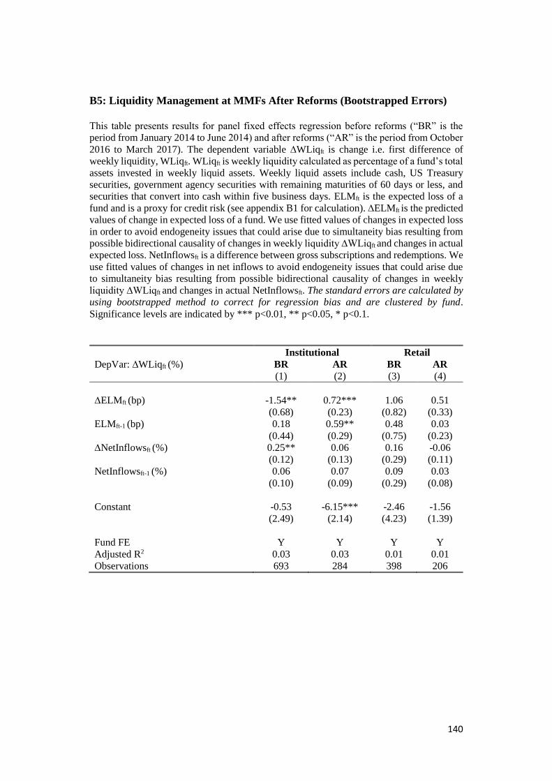
140

B5: Liquidity Management at MMFs After Reforms (Bootstrapped Errors)

This table presents results for panel fixed effects regression before reforms (“BR” is the

period from January 2014 to June 2014) and after reforms (“AR” is the period from October

2016 to March 2017). The dependent variable ∆WLiqft is change i.e. first difference of

weekly liquidity, WLiqft. WLiqft is weekly liquidity calculated as percentage of a fund’s total

assets invested in weekly liquid assets. Weekly liquid assets include cash, US Treasury

securities, government agency securities with remaining maturities of 60 days or less, and

securities that convert into cash within five business days. ELMft is the expected loss of a

fund and is a proxy for credit risk (see appendix B1 for calculation). ∆ELMft is the predicted

values of change in expected loss of a fund. We use fitted values of changes in expected loss

in order to avoid endogeneity issues that could arise due to simultaneity bias resulting from

possible bidirectional causality of changes in weekly liquidity ∆WLiqft and changes in actual

expected loss. NetInflowsft is a difference between gross subscriptions and redemptions. We

use fitted values of changes in net inflows to avoid endogeneity issues that could arise due

to simultaneity bias resulting from possible bidirectional causality of changes in weekly

liquidity ∆WLiqft and changes in actual NetInflowsft. The standard errors are calculated by

using bootstrapped method to correct for regression bias and are clustered by fund.

Significance levels are indicated by *** p<0.01, ** p<0.05, * p<0.1.

Institutional Retail

DepVar: ∆WLiqft (%) BR AR BR AR

(1) (2) (3) (4)

∆ELMft (bp) -1.54** 0.72*** 1.06 0.51

(0.68) (0.23) (0.82) (0.33)

ELMft-1 (bp) 0.18 0.59** 0.48 0.03

(0.44) (0.29) (0.75) (0.23)

∆NetInflowsft (%) 0.25** 0.06 0.16 -0.06

(0.12) (0.13) (0.29) (0.11)

NetInflowsft-1 (%) 0.06 0.07 0.09 0.03 (0.10) (0.09) (0.29) (0.08)

Constant -0.53 -6.15*** -2.46 -1.56

(2.49) (2.14) (4.23) (1.39)

Fund FE Y Y Y Y

Adjusted R2 0.03 0.03 0.01 0.01

Observations 693 284 398 206

141

B6: Liquidity Management at MMFs After 2016 Amendments (Different Lag

specification for fitted values of contemporaneous variables - 7 lags)

This table presents results for panel fixed effects regressions before reforms (“BR” is the

period from January 2014 to June 2014) and after reforms (“AR” is the period from October

2016to March 2017). The dependent variable ∆WLiqft the first difference of weekly

liquidity, WLiqft. WLiqft is weekly liquidity calculated as percentage of a fund’s total assets

invested in weekly liquid assets. Weekly liquid assets include cash, US Treasury securities,

government agency securities with remaining maturities of 60 days or less, and securities

that convert into cash within five business days. ELMft is the expected loss of a fund and is

a proxy for credit risk (see appendix B1 for calculation). ∆ELMft is the predicted value of

change in expected loss of a fund. We use fitted values of change in expected loss in order

to avoid endogeneity issues that could arise due to simultaneity bias resulting from possible

bidirectional causality of changes in weekly liquidity ∆WLiqft and changes in expected loss,

ELMft. NetInflowsft is a difference between gross subscriptions and redemptions. We use

fitted values of ∆NetInflowsft to avoid endogeneity issues that could arise due to simultaneity

bias resulting from possible bidirectional causality of changes in weekly liquidity, ∆WLiqft

and changes in net inflows, ∆NetInflowsft. The standard errors are clustered by fund.

Significance levels are indicated by *** p<0.01, ** p<0.05, * p<0.1.

Institutional Retail

DepVar: ∆WLiqft (%) BR AR BR AR

(1) (2) (3) (4)

∆ELMft (bp) -0.99** 0.60** 1.05* 0.81

(0.48) (0.29) (0.63) (0.58)

ELMft-1 (bp) 0.32 0.64*** 0.39 0.15

(0.26) (0.23) (0.36) (0.28)

∆NetInflowsft (%) 0.28** 0.14* 0.37 -0.02

(0.12) (0.08) (0.25) (0.17)

NetInflowsft-1 (%) 0.09 0.11 0.31 0.06 (0.12) (0.08) (0.29) (0.17)

Constant -1.18 -6.26*** -1.92 -2.27

(1.38) (1.67) (2.01) (2.19)

Fund FE Y Y Y Y

Adjusted R2 0.03 0.04 0.02 0.03

Observations 693 284 398 206

142

B7: Shareholders’ Response to 2016 Amendments (Bootstrapped Errors)

This table presents results for panel fixed effects regressions before reforms (“BR” is the

period from January 2014 to June 2014) and after reforms (“AR” is the period from October

2016 to March 2017). The dependent variable is NetInflowsft, calculated as a difference

between gross subscriptions and redemptions of a fund. ELMft is the expected loss of a fund

and is a proxy for credit risk (see appendix B1 for calculation). ∆ELMft is the predicted

values of changes in loss of a fund. We use fitted values of change in expected loss in to

avoid endogeneity which could lead to simultaneity bias resulting from possible

bidirectional causality of NetInflowsft and changes in expected loss. WLiqft is the weekly

liquidity calculated as total weekly liquid assets of a fund as a percentage of its total assets.

Weekly liquid assets include cash, US treasury securities, government agency securities with

remaining maturities of 60 days or less, and securities that convert into cash within five

business days. ∆WLiqft is the predicted values of the changes in the weekly liquidity of a

fund. We use fitted values of ∆WLiqft to avoid endogeneity issues that could arise from

possible bidirectional causality of changes in weekly liquidity, ∆WLiqft and net inflows,

NetInflowsft. We additionally control but do not report the following variables: NetYieldft

which is the value-weighted average of the 7-day net yields of fund classes as reported on

N-MFP form. This represents the difference between the gross yield of portfolio less

management fee. ExRatioft which is the expense ratio of a fund calculated as the difference

between gross yield (a fund’s portfolio yield) and net yield (the yield paid to a fund’s

investor). Sizeft calculated as the log of total net assets of a fund. The standard errors are

calculated by using bootstrapped method to correct for regression bias and are clustered by

fund. Significance levels are indicated by *** p<0.01, ** p<0.05, * p<0.1.

Institutional Retail

DepVar: NetInflowsft (%) BR AR BR AR

(1) (2) (3) (4)

∆ELMft (bp) -0.22 -1.17*** -0.47 -0.40

(0.52) (0.45) (0.72) (0.48)

ELMft-1 (bp) -0.40 -0.45 -1.18** -0.28

(0.62) (0.32) (0.59) (0.27)

∆WLiqft (%) 0.10 -0.03 0.13 -0.00

(0.13) (0.13) (0.21) (0.17)

WLiqft -1 (%) 0.04 -0.16** -0.08 -0.02

(0.08) (0.08) (0.12) (0.08)

Constant -2.78 0.96 5.34 -11.98

(6.93) (8.80) (7.98) (8.62)

Fund FE Y Y Y Y

Controls Y Y Y Y

Adjusted R2 0.03 0.10 0.04 0.01

Observations 606 291 359 209

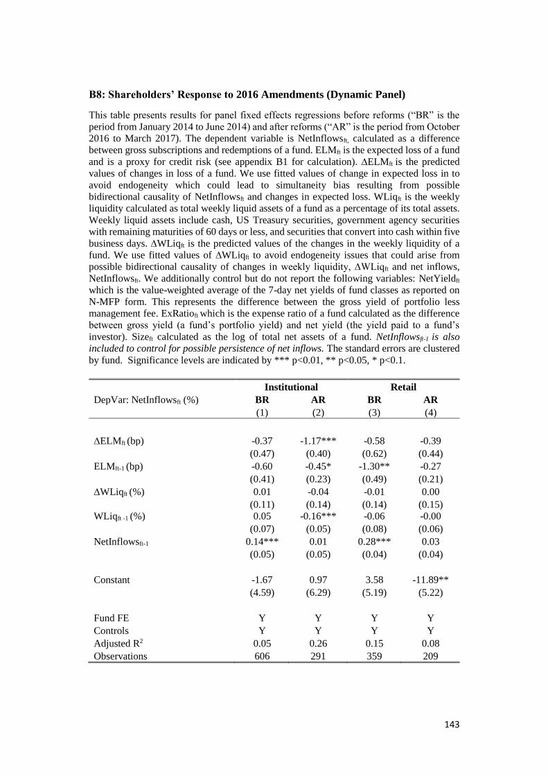
143

B8: Shareholders’ Response to 2016 Amendments (Dynamic Panel)

This table presents results for panel fixed effects regressions before reforms (“BR” is the

period from January 2014 to June 2014) and after reforms (“AR” is the period from October

2016 to March 2017). The dependent variable is NetInflowsft, calculated as a difference

between gross subscriptions and redemptions of a fund. ELMft is the expected loss of a fund

and is a proxy for credit risk (see appendix B1 for calculation). ∆ELMft is the predicted

values of changes in loss of a fund. We use fitted values of change in expected loss in to

avoid endogeneity which could lead to simultaneity bias resulting from possible

bidirectional causality of NetInflowsft and changes in expected loss. WLiqft is the weekly

liquidity calculated as total weekly liquid assets of a fund as a percentage of its total assets.

Weekly liquid assets include cash, US Treasury securities, government agency securities

with remaining maturities of 60 days or less, and securities that convert into cash within five

business days. ∆WLiqft is the predicted values of the changes in the weekly liquidity of a

fund. We use fitted values of ∆WLiqft to avoid endogeneity issues that could arise from

possible bidirectional causality of changes in weekly liquidity, ∆WLiqft and net inflows,

NetInflowsft. We additionally control but do not report the following variables: NetYieldft

which is the value-weighted average of the 7-day net yields of fund classes as reported on

N-MFP form. This represents the difference between the gross yield of portfolio less

management fee. ExRatioft which is the expense ratio of a fund calculated as the difference

between gross yield (a fund’s portfolio yield) and net yield (the yield paid to a fund’s

investor). Sizeft calculated as the log of total net assets of a fund. NetInflowsft-1 is also

included to control for possible persistence of net inflows. The standard errors are clustered

by fund. Significance levels are indicated by *** p<0.01, ** p<0.05, * p<0.1.

Institutional Retail

DepVar: NetInflowsft (%) BR AR BR AR

(1) (2) (3) (4)

∆ELMft (bp) -0.37 -1.17*** -0.58 -0.39

(0.47) (0.40) (0.62) (0.44)

ELMft-1 (bp) -0.60 -0.45* -1.30** -0.27

(0.41) (0.23) (0.49) (0.21)

∆WLiqft (%) 0.01 -0.04 -0.01 0.00

(0.11) (0.14) (0.14) (0.15)

WLiqft -1 (%) 0.05 -0.16*** -0.06 -0.00

(0.07) (0.05) (0.08) (0.06)

NetInflowsft-1 0.14*** 0.01 0.28*** 0.03

(0.05) (0.05) (0.04) (0.04)

Constant -1.67 0.97 3.58 -11.89**

(4.59) (6.29) (5.19) (5.22)

Fund FE Y Y Y Y

Controls Y Y Y Y

Adjusted R2 0.05 0.26 0.15 0.08

Observations 606 291 359 209

144

B9: Shareholders’ Response to 2016 Amendments (Different Lag specification

for fitted values of contemporaneous variables - 7 lags)

This table presents results for panel fixed effects regressions before reforms (“BR” is the

period from January 2014 – June 2014) and after reforms (“AR” is the period from October

2016 – March 2017). The dependent variable is NetInflowsft, calculated as a difference

between gross subscriptions and redemptions of a fund. ELMft is the expected loss of a fund

and is a proxy for credit risk (see appendix B1 for calculation). ∆ELMft is the predicted

values of changes in loss of a fund. We use fitted values of change in expected loss in to

avoid endogeneity which could lead to simultaneity bias resulting from possible

bidirectional causality of NetInflowsft and changes in expected loss. WLiqft is the weekly

liquidity calculated as total weekly liquid assets of a fund as a percentage of its total assets.

Weekly liquid assets include cash, US treasury securities, government agency securities with

remaining maturities of 60 days or less, and securities that convert into cash within five

business days. ∆WLiqft is the predicted values of the changes in the weekly liquidity of a

fund. We use fitted values of ∆WLiqft to avoid endogeneity issues that could arise from

possible bidirectional causality of changes in weekly liquidity, ∆WLiqft and net inflows,

NetInflowsft. We additionally control but do not report the following variables: NetYieldft

which is the value-weighted average of the 7-day net yields of fund classes as reported on

N-MFP form. This represents the difference between gross yield of portfolio less

management fee. ExRatioft which is the expense ratio of a fund calculated as the difference

between gross yield (a fund’s portfolio yield) and net yield (the yield paid to a fund’s

investor). Sizeft calculated as the log of total net assets of a fund. The standard errors are

clustered by fund. Significance levels are indicated by *** p<0.01, ** p<0.05, * p<0.1.

Institutional Retail

DepVar: NetInflowsft (%) BR AR BR AR

(1) (2) (3) (4)

∆ELMft (bp) 0.02 -0.68* -0.91 -0.07

(0.43) (0.39) (0.60) (0.42)

ELMft-1 (bp) -0.33 -0.28 -1.25*** -0.14

(0.42) (0.27) (0.46) (0.21)

∆WLiqft (%) 0.19* -0.07 0.03 0.25

(0.10) (0.09) (0.17) (0.15)

WLiqft -1 (%) 0.09 -0.13*** -0.11 0.02

(0.06) (0.05) (0.10) (0.06)

Constant -4.41 -4.19 6.92 -13.83**

(4.18) (5.75) (5.62) (5.83)

Fund FE Y Y Y Y

Controls Y Y Y Y

Adjusted R2 0.02 0.27 0.02 0.09

Observations 583 278 346 201

145

Chapter 5 A New Performance Indicator for Money

Market Funds

5.1 Introduction

Since October 2016, institutional MMFs, which serve a more volatile shareholder

base than retail MMFs, have floated their net asset value (NAV) and operated

separately from the more stable retail funds. This has stripped money-like features

from institutional MMFs. This is a new characteristic that has not been studied

extensively before. It is interesting to explore how floating NAV affects the risk-

taking of funds and the response of shareholders to it. This chapter specifically

focuses on exploring the drivers of NAV, the impact of floating NAV on risk-taking

of funds and investors’ response to floating NAV.

This paper fills a gap in the literature since it is, to the best of our knowledge, the

first to explore how floating NAV for institutional prime funds influences the

characteristics of the funds after their complete segregation from retail prime funds.

Utilizing a unique dataset, we explore how shareholders of money market funds react

to floating NAV. We also explore how portfolio characteristics influence the NAV

of funds.

Our contributions to the literature are as follows. First, we contribute to the

existing performance-flow literature of money market funds (Sirri and Tufano 1998;

Koppenhaver and Sapp 2005; Chernenko and Sunderam 2014) which established a

positive relationship between yield and net inflows. A key novelty of our paper is

that we identify a new indicator of performance, the floating NAV, which is now

used particularly by institutional investors. We show that MMFs with higher floating

146

net asset value attract more inflows. In fact, they actively shift their investments to

funds that offer higher potential for capital gains as compared to other MMFs. So,

MMFs have an incentive to increase their net asset value.

Second, we add to the literature that deals with factors influencing returns of

money market funds. Domian and Reichenstein (1998) argue that a fund’s return is

determined by the size of the expense ratio. Koppenhaver (1999) shows that along

with expenses, portfolio characteristics also affect returns. We explore the factors

that influence the newly introduced source of return, capital gains from floating

NAV, which has not been studied before. We find that portfolio risk and the higher

weighted average of a fund has a positive effect on NAV. But, a higher proportion

of liquid assets leads to lower NAV. These results imply that to offer higher capital

gains a fund must hold a riskier portfolio mix.

Third, our study contributes to the literature on the impact of the introduction of the

floating NAV on money funds and investor behaviour. Some studies focus on the

effect of floating NAV on runs. Gordon and Gandia (2014) and Witmer (2016)

suggest that it does not eliminate run-like behaviour while Hanson et al. (2015) argue

that it successfully removes strategic motives to run. Other studies investigate its

influence on the risk-taking behaviour of funds. For instance, Hanson et al. 2015

argue that it does not remove ex-ante risk-taking incentives. Parlatore (2016) studies

the consequences of the adoption of a floating NAV among other new regulations

using a tournament model. The paper states that adopting floating NAV for the whole

industry could boost the total supply of liquidity because investors would be attracted

to MMFs as they can earn returns from floating NAV. But the risk should be kept

low by restraining asset price volatility. La Spada (2018) also proposes a novel

147

tournament model to study whether competition over relative performance generates

reach for yield in a low risk-free rate environment. La Spada conducts empirical

analysis over the January 2002 to August 2008 period to confirm the predictions of

the model relating to risk-taking of MMFs. The paper argues that requiring

institutional prime MMFs to adopt a floating NAV, could lead institutional prime

MMFs to take on more risk in a low policy rate environment. Furthermore, for stable

NAV funds, if the regulator externally imposes a cost on MMFs that break the stable

NAV, the model predicts that this would reduce the risk taking of all MMFs. These

studies are based on the period prior to the actual implementation of the new SEC

rules and are lacking empirical analysis after the reforms. The only paper that

performs empirical analysis after reforms is Li et al (2018), who document the impact

of the NAV flotation introduced for institutional funds. They find that during the

months around and just after the reform took effect, institutional funds engaged in

less risk-taking than retail funds by decreasing interest rates, liquidity and credit risk.

This resulted in lower yields and NAVs and less volatile NAVs. But this difference

faded through 2017 when institutional funds increased their risk-taking to pre-reform

levels. Li et al. (2018) focus on the evolution of risk-taking of MMFs during reforms.

By contrast, we explore risk-taking incentives of MMFs after reforms. Using actual

floating NAV data, we empirically show that the introduction of floating NAV has

two competing effects on risk-taking of money market funds, one risk-increasing and

the other risk-limiting. On the one hand, to attract investors, a fund must increase

portfolio risk. This suggests that floating NAV has not altered incentives to chase

risk. On the other hand, to keep investors, a fund must select the portfolio mix

148

cautiously to limit NAV volatility because investors withdraw from funds whose

NAV fluctuates excessively.

Fourth, we expand the existing literature about runs on constant NAV money

market funds which find that runs are more intense for less liquid funds (Wermers

2011; Jank and Wedow 2015), funds with higher sponsor risk (Schmidt et al. 2016)

and higher credit risk (Chari and Jagannathan 1988; Jacklin and Bhattacharya 1988;

Chernenko and Sunderam 2014). In addition, these studies show that the funds that

cater to institutional investors (Wermers 2011; Schmidt et al 2016; Chernenko and

Sunderam 2014) undergo stronger run episodes. The 2016 Amendments mandate

that institutional investors cannot invest in constant NAV funds anymore, so we

explore the possibility of instability in such funds. We show that investors in constant

NAV funds (i.e. retail investors) actively track the shadow NAV of their fund and

tend not to remain in funds that have a more volatile shadow NAV. This is because

of the risk of such a fund to breach the par value threshold and result in loss of

principal. This implies that the constant NAV (retail) funds after complete

segregation from institutional funds may still be subject to runs when in distress.

The rest of the paper proceeds as follows: Section 5.2 discusses the regulatory

landscape of this study. Section 5.3 describes the data. Section 5.4 presents the

empirical analysis and results. Section 5.5 concludes.

149

5.2 Regulatory Landscape

During the global financial crisis and sovereign debt crisis, prime money market

funds proved vulnerable to financial shocks and are now considered to add fragility

to the financial system. During these events, institutional prime funds were more

likely to undergo heavy redemption pressure than retail prime funds. This is because

institutional investors have larger investments at risk and better access to resources

for monitoring fund performance (Schapiro 2012). Moreover, they understand that

they can lower exit costs if they redeem before others should liquidity dry up

(McCabe 2010). Consequently, rule 2a-7 was amended in 2014 (amendments

became effective in October 2016) to attenuate run risk among institutional funds.

Before the reform, a fund could have both retail and institutional share classes.

The new rules have fully segregated institutional funds from retail funds, which

means that a single fund can offer shares to either retail31 shareholders or institutional

shareholders, but not both. Since their inception, MMFs have operated under a

special provision in rule 2a-7 which allowed them to maintain a stable NAV of $1.00

by using the amortized cost method to value individual securities and the penny

rounding method to value fund shares. This has changed for institutional funds,

which are now required to trade at floating net asset value. This means that a fund

must use market-based values of their securities to value their portfolio so that the

daily share prices of the funds now fluctuate with the market. This change addresses

the first-mover advantage that institutional investors usually gain at the expense of

31A retail money market fund, under 2016 Amendments, is defined as a fund that has policies and

procedures which would limit beneficial investors of the fund to natural persons (SEC 2014).

150

retail investors, during a crisis. Sceptics remain unconvinced about the ability of

floating NAV to have much effect on the risk of runs (Gordon and Gandia 2014;

Witmer 2016). They claim that the incentive to withdraw early from a fund remains

the same or might even lead to pre-emptive runs. The way events unfold in a distress

period remains yet to be seen. Government and retail money market funds continue

to use the amortized cost method and/or penny rounding method to maintain a stable

NAV.

The new rules have consequences for shareholders of MMFs. Before the SEC

reforms following the global financial crisis, all MMFs were higher yielding

investments than bank deposits while retaining deposit-like features such as same-

day redemption and preservation of capital. Now, shareholder redemptions in

institutional prime funds trading at floating NAV may incur a gain or a loss in capital.

This led to shareholders shifting their money from prime to government funds.

However, many of these funds remained institutional funds. It is of great interest to

observe the behaviour of the investors who choose to remain in institutional prime

funds. We limit out analysis to prime money market funds because these are the

funds that are affected more by the reforms and are considered to be a source of

instability.

5.3 Data Description

We create a unique dataset comprising detailed portfolio holdings of US prime

money market funds which are filed monthly with the Securities and Exchange

Commission. These filings are publicly available from the SEC EDGAR database.

151

The amendments to rule 2a-7 that were introduced in May 2010 require MMFs

to file a monthly report on the N-MFP form, which includes a detailed schedule of

portfolio holdings of money market funds, starting from November 2010. From April

2016, the reporting of additional information is required under the new version of

the form (N-MFP2). Our sample includes information from both versions of the

form. Both forms provide information about fund-level variables like total net assets,

type of fund, gross yield, net yield and monthly shareholders subscriptions and

redemptions. In addition, for each security held, these report issuer name, amount of

principal, type of instrument, yield, legal maturity date and the CUSIP number. The

N-MFP2 form additionally reports daily and weekly liquidity, floating net asset

value, target net asset value and type of shareholder base.

Our final dataset ranges from January 2013 to April 2018. Most of the analysis

focuses on the after-reform period which starts from the compliance month, October

2016, and ends in April 2018, which is the latest date the data was avaiable at the

time of analysis. In figures, we utilize the before-reform period which starts from

January 2013 and ends July 2014, the month of the announcement of 2016

Amendments. The number of months is selected to get before- and after-reform

periods of equal length. We conduct our analysis by analysing retail prime money

market funds and institutional prime money market funds separately. The funds that

report themselves as “retail exempt” funds are called retail prime money market

funds and the remaining funds are institutional prime money market funds.

152

5.4 Empirical Results

The institutional funds have floated their NAV since October 2016. Retail funds

still maintain a constant NAV. For institutional investors, the floating NAV has

introduced previously non-existent risk of losing the principal. So, post reform,

institutional investors must be more cautious of the NAV of the MMF portfolio like

any other mutual fund investor. Many funds have converted into government money

market funds, which have no such requirement. Others have decided to stay in the

prime money market funds. Our analysis focuses on exploring the behaviour of

investors that have remained in the prime fund industry. We explore institutional

prime funds’ performance-flow sensitivity based on a new measure of performance,

the floating NAV. In addition, we identify factors that influence the magnitude and

fluctuations in NAV.

5.4.1 Descriptive Statistics

Table 5.1 reports summary statistics for prime funds in the before-reform (BR)

period, from January 2013 to July 2014, and after-reform (AR) period, from October

2016 to April 2018. Panel A presents statistics for institutional prime funds. In our

sample, we have 149 institutional prime funds before reforms which drop to 77 funds

after reforms. After reforms, the median institutional fund has approximately $1.39

billion in total net assets, but the distribution is positively skewed with a mean of

$7.36 billion. Furthermore, the median fund’s NAV moves upward by one basis

point from their target NAV, which is a small movement considering that these funds

are using floating NAV. Panel B reports statistics for retail prime funds. Our data

153

includes 94 retail prime funds before reforms and 41 retail prime funds after reforms.

The median retail prime fund manages about $0.89 billion of net assets with average

net assets of $5.87. This indicates the presence of some very large funds. The median

retail fund’s NAV movement is very similar to that of institutional funds. We plot

the distribution of NAV changes to explore its characteristics. Figure 5.1 shows the

box and whiskers plot of the distribution of NAV changes for institutional prime

money market funds in the before-reform and after-reform periods. Before-reforms

the NAV remains within a narrow range, moving only one basis point in each

direction. However, there are several outliers indicating that some funds took on

more risk and let their NAV fall by up to 18 bps. After reforms, the distribution of

NAV changes becomes wider with values ranging from –4 bps to +8 bps, which is

to be expected because funds use floating NAV and can let their values move away

from the target NAV without fear of having to break the buck and liquidate a fund.

We see that the majority of times funds’ NAV moves upward while there are some

funds whose NAV moves downward. This drop in NAV happens only for 25 percent

of the funds during the early months after switching to floating NAV. Interestingly,

as more time goes by since the introduction of floating NAV, especially since

January 2018, about 50 percent of the funds have negative movements in NAV which

may indicate that funds are becoming less concerned about downward NAV

adjustments.

Retail prime funds need to keep a constant NAV even after the 2016

Amendments. Like institutional prime funds they have a very narrow range of

movement in (shadow) NAV (Figure 5.2) before reforms. But they are characterized

154

by several instances of relatively large NAV variations, where in some cases it drops

by –23 bps. Still they stay well above the –50 bps threshold of acceptable movement

in NAV breaching which requires a fund to break the buck and possibly face

liquidation. After reforms, retail funds, in line with institutional funds, also have

wider NAV distribution where NAV moves between -4 bps to +8 bps. However,

there is a reduction in outliers. This more liberal movement could be due to the

complete segregation of retail prime funds from institutional funds. However,

because of several changes in MMFs taking place simultaneously, there might be

other factors contributing to the reduction in outliers. In any case, retail prime funds

have a more stable shareholder base than before, which gives them an opportunity to

take on more risk without adverse consequences.

Finally, we observe that before reforms institutional prime funds have higher

volatility in NAV than retail prime funds.32 However, after reforms, institutional

prime funds restrain NAV fluctuations. This indicates that they are more cautious

about the extent of the movements in the NAV as they must now float the NAV, and

higher deviations could lead to investor withdrawals.

5.4.2 Drivers of NAV

We start our analysis by investigating the portfolio characteristics that influence

the net asset value of a fund. This would inform the actions that an institutional fund

32 To ensure that this is empirically verifiable, we calculate differences in averages of NAV volatility

between retail and institutional prime fund, before and after reforms. On average, before reforms

institutional prime funds have 0.15 basis points higher volatility than retail prime funds, whereas after

reforms they have 0.21 basis points lower NAV volatility (NAV volatility is calculated as rolling

standard deviation of a fund’s NAV over a fixed window of the past six-months).

155

can take to rein in the floating NAV and keep it within an acceptable range for

investors. We estimate the following monthly panel fixed effects regression,

NAVMft = αf + β1 FlowVolft-1+ β2 Spreadft-1+ β3 WALft-1 + β4 Sizeft-1 +

β5 FFSizeft-1 + β6 NetYieldft-1 + εft eq. (1)

where the dependent variable NAVMft is the difference between actual NAV and the

target NAV as a percentage of target NAV, which captures the potential of a fund to

generate a capital gain/loss. αf are fund fixed effects to control for unobserved fund

characteristics. The extent of unpredictable investors’ redemption patterns can

influence a fund’s NAV because to meet unexpected withdrawals a fund must sell

its portfolio of securities, which affects its net asset value (Nanda et al. 2000; Chen

et al. 2010). Unpredictable redemption behaviour is captured by FlowVolft, which is

flow volatility calculated as the 6-month rolling standard deviation of NetInflowsft.

NetInflowsft is the difference between monthly subscriptions and redemptions as a

percentage of the lagged total net assets of a fund. Spreadft is a fund’s portfolio gross

yield net of the average government money market funds’ gross yield, a proxy for

portfolio risk. We include a measure of portfolio maturity, WALft, which is the

weighted average life, calculated as average days to maturity weighted by the

investment weight of each security. In some regressions, we include WLiqft instead

of WALft. WALft and WLiqft are highly correlated so they are not used together to

avoid multicollinearity issues. WLiqft is weekly liquidity calculated as percentage of

a fund’s total assets invested in weekly liquid assets. Weekly liquid assets are cash,

US Treasury securities, government agency securities with remaining maturities of

60 days or less, and securities that convert into cash within five business days. We

control for the size of a fund and its family, that is a group of funds owned by the

156

same manager. Sizeft is the log of total net assets of a fund. FFSizeft is the log of total

net assets of a fund family. We add net yield to assess its relationship with capital

gains. NetYieldft is the yield earned by funds’ shareholders, calculated as the value-

weighted average of the 7-day net yields of fund share classes as reported on N-MFP

form. All variables are lagged by one month. We cluster standard errors by fund.

Table 5.2 contains the regression results for eq. (1). In Column 1, the coefficient

of Spreadft is positive and significant indicating that institutional prime funds with

riskier portfolios have more potential for capital gains. Similarly, the funds with

longer maturity securities have bigger NAVMft and therefore higher capital gains.

On the contrary, the funds with more liquid portfolio (Column 2) have lower

NAVMft because the funds with higher proportion of very short-term securities do

not move up as compared to the ones with longer maturities. These results imply that

the funds must invest in riskier securities to increase the floating NAV of their funds

to boost their performance. The funds that belong to bigger fund families tend to

have lower NAVMft. This could have two explanations. First, it could be that the

funds that belong to bigger fund families have a more cautious attitude towards

excessive risk-taking to avoid bad reputation in case the market value of a portfolio

security goes down. Second, they could have invested in riskier securities whose

market value has plunged.

Interestingly, the funds with higher NetYieldft have lower NAVMft possibly

because the funds are using the increases in floating NAV as an alternative form of

compensation. So, if a fund is providing larger capital gains they seem to pay lower

yields to the investors. This has consequences for expense ratios charged by funds.

Usually the funds waive their management fee to offer higher yields, but if the

157

investors subscribe to funds because of potential for capital gains they could charge

higher expenses while still attracting inflows. However, this potential for funds to

earn a higher fee is limited because the returns from net yield is much higher than

that from capital gains. But the investors could opt for funds offering higher capital

gains for deferred tax purposes.

In Column 3, retail prime funds with riskier portfolio have higher NAVMft,

however, this significance is not robust and disappears in Column 4 when we control

for liquidity of a fund. They do not seek to increase their risk and portfolio maturity

to increase their NAV because they trade at a stable share price and therefore cannot

attract retail investors by differentiating themselves on capital gains. Like

institutional funds, retail funds with more liquid portfolios have lower NAVMft.

Overall, we document that net asset value of a fund is influenced by portfolio

characteristics such as portfolio risk, average portfolio maturity and fund liquidity.

To increase NAV, in order to provide higher capital gains, a fund must increase its

portfolio risk, hold less liquid longer maturity assets which could put a fund in

distress in a time of crisis.

5.4.3 Risk from Floating NAV

The extent of fluctuation in floating NAV is of importance to investors because

it is an indicator of the stability of a fund’s performance. Greater NAV volatility

means higher risk of incurring a capital loss. Therefore, it is valuable to investigate

the factors that influence the NAV volatility.

158

We estimate the following panel fixed effects regression,

NAVVolft = αf + β1 FlowVolft-1+ β2 Spreadft-1+ β3 WALft-1 + β4 Sizeft-1 +

β5 FFSizeft-1 + β6 NetYieldft-1 + εft eq. (2)

where the dependent variable NAVVolft is NAV volatility calculated as rolling

standard deviation of NAV over a six-month fixed window. It is a proxy for the risk

of loss from investing in a floating NAV. Our main explanatory variables are flow

volatility, FlowVolft and portfolio risk, Spreadft, defined as before. The uncertainty

in redemptions of shareholders can lead to more volatility in net asset value. Riskier

portfolio can influence the volatility of portfolio value as evident from our previous

findings. We control for weighted average life, WALft fund size, Sizeft fund family

size, FFSizeft and net yield, NetYieldft of a fund which are defined as before. As in

the previous specification, in some regressions, we include WLiqft of a fund, while

avoiding to use WALft and WLiqft together to avoid multicollinearity issues. We

include fund fixed effects in all regressions and cluster standard errors at fund level.

Table 5.3 shows the estimation results for eq. (2). We find that both institutional

and retail prime funds with higher flow volatility have more NAV volatility. This is

because the funds with higher unpredictability in net inflows must sell their securities

on short-notice, which affects the net asset value, and therefore leads to higher

unpredictability in the NAV of a fund. Greater unpredictability in NAV denotes

elevated risk of capital loss. This means that in the event of a crisis, when investors

redeem ferociously it would deteriorate the value of NAV further, which would lead

to more outflows, hence creating a feedback loop. Furthermore, institutional prime

funds that carry more portfolio risk, Spreadft have greater variability in NAV because

159

the market value of riskier securities fluctuates more, leading to greater risk of capital

loss. To restrict the risk of capital losses institutional funds must rein in their risk-

taking and seek to create a more stable shareholder base by taking appropriate

measures. In the next sections we investigate factors that influence the behaviour of

shareholders, to learn more about the steps a fund must take to retain shareholders.

5.4.4 Shareholders’ Response to Floating NAV

For institutional investors, the floating NAV has introduced a previously non-

existent opportunity for capital gains and a possible risk of incurring losses on

redemptions. So, we next examine the response of shareholders to movement in

NAV and the risk of losing principal associated with possible negative changes in

NAV. We run the following panel fixed effects regression:

NetInflowsft = αf + β1 NAVMft-1 + β2 NAVVolft-1 + β3 NetYieldft-1 + β4 Wliqft-1 +

β5 ExRatioft-1 + β6 Sizeft-1 + β7 FFSizeft-1 + β8 NetInflowsft-1 + εft eq. (3)

where NetInflowsft is calculated as a difference between monthly subscription and

redemptions as a percentage of lagged total net assets of a fund. αf represents fund

fixed effects. Our main explanatory variables are movement in NAV, NAVMft and

NAV volatility, NAVVolft. NAVMft captures the potential of a fund to produce a

capital gain/loss. NAVVolft is a proxy for the risk of capital loss from investing in a

floating NAV. We use it to test the response of investors to funds whose NAV

changes a lot. We control for other factors that might impact the investment decision

of investors such as net yield, NetYieldft, weekly liquidity, WLiqft, size of a fund,

Sizeft and fund family size, FFSizeft. We also include ExRatioft, which is the expense

ratio of a fund calculated as the difference between the gross yield and the net yield

160

of a fund. We include the lagged dependent variable, NetInflowsft to control for

persistence of net inflows (Domian and Reichenstein 1998; Christoffersen and Musto

2002). Standard errors are clustered by fund.

Table 5.4 presents the regression results for both retail and institutional prime

funds. Column 1 shows the results for institutional prime funds. The coefficient of

NAVMft is positive and significant. NAVMft is a measure of the potential of a fund

to offer capital gains on an investment. An increase in NAV results in capital gains,

while decrease in NAV could lead to loss in the value to principal invested. We find

that money market funds with higher NAVMft attract more inflows. This implies that

the institutional investors i) seek to invest in funds that offer higher capital gains, ii)

and use NAV to assess the performance of funds. These results add to the existing

literature on performance-flow relationship by documenting a new performance

measure that the investors seem to have adopted to differentiate money market funds.

This relationship between flow and floating NAV has not been studied before. As

expected, the funds with higher yield, NetYieldft have more net inflows, NetInflowsft,

which is a well-established relationship in previous studies (Christoffersen 2001;

Christoffersen and Musto 2002; Kacperczyk and Schnabl 2013; Chernenko and

Sunderam 2014). NetYieldft continues to be the primary indicator of performance33

and explains higher degree of variation in net inflows as compared to movement in

NAV, NAVMft which makes sense because the returns earned from NAVMft stay

within a very narrow range.

33 In unreported univariate regressions, we find that R-squared for NetYieldft is higher than that of

NAVMft.

161

The floating NAV can lead to losses. So, we investigate how investors react to

the volatility of NAV. A fund with higher volatility in NAV presents increased risk

of capital losses. As expected, the coefficient of NAV volatility, NAVVolft is

negative and significant indicating that a fund with higher NAV volatility tends to

have lower net inflows. The investors avoid the funds that might drive their capital

to take a plunge. The investors are watchful of the risks associated with the floating

NAV. This behaviour is consistent with the literature that recognizes that

institutional shareholders have greater capital at risk, therefore they tend to monitor

the risks and returns of a fund portfolio (Schapiro 2012). Overall, this shows that

while the investors are searching for higher returns they are doing so with caution

and weigh the risks associated with the prospective gains from the floating NAV.

Our control variables have expected signs and significance. We find that the

lagged weekly liquidity, WLiqft is negative and highly significant which is consistent

with Jank and Wedow’s (2015) findings that MMFs with more liquid assets tend to

have lower inflows. This is possibly because the investors, once confident about the

safety of the funds, tend to withdraw from funds with higher liquidity because that

results in lower yields. Next, the coefficient of expense ratio, ExRatioft is negative

and significant. This shows that institutional investors are sensitive to the cost of

investment in the money market funds. The institutional investors withdraw money

from the funds that have higher expense ratios because this leads to lower yields.

Further, we control for size of a fund, Sizeft and its family, FFSizeft. Both coefficients

are insignificant showing that the investors do not regard size of a fund or its sponsor

as a major factor in their investment decisions. We also include lagged dependent

162

variable to account for persistence of NetInflowsft. The coefficient is positive and

significant showing persistence in fund net inflows.

In Column 2, we repeat the analysis for retail prime funds. The coefficients of

NAVMft and NAVVolft are not significant indicating that the funds do not take the

value of NAV into account when making investment decisions. This is

understandable as the retail prime funds trade on a target NAV of $1.00, even if the

shadow NAV (i.e. fair value of portfolio divided by number of shares, as reported on

N-MFP form) is higher or lower than the target NAV. Unlike institutional funds,

retail funds do not have significant inflows with higher NAVMft. This is expected

because retail funds keep using stable NAV. Therefore, investors redeem the

principal at stable NAV and have no possibility of capital gain. However, these

investors are attracted to higher yielding funds as seen from a positive and significant

coefficient of NetYieldft. Because retail investors do not have a possibility of loss

when they trade, NAV volatility, NAVVolft does not have a significant impact these

funds. Next, the control variable WLiqft is negative and significant indicating that

retail investors withdraw their money from the funds with higher proportion of liquid

assets, which is plausible because this leads to lower yields. Interestingly, in contrast

to institutional counterpart, the coefficient of ExRatioft is positive and significant

demonstrating that the retail investors tend to invest more in funds with higher

expense ratios.

One explanation could be that the retail investors, having lower resources to track

a fund’s portfolio, put more confidence in the funds with higher expense ratios

because such funds are deemed to be managed actively (Morningstar 2015). We also

include lagged dependent variable to account for persistence of NetInflowsft. As

163

expected, the coefficient is positive and significant showing persistence in fund net

inflows.

In short, institutional investors seek funds with higher capital gains but avoid

funds with higher propensity for incurring capital losses. This behaviour is not

observed in retail prime funds who do not have option to earn capital gains from their

investments in money market funds.

5.4.5 MMF Shareholders Seek Capital Gains

We next investigate whether investors actively shift between prime funds based

on capital gains incentives - an action consistent with chasing higher yields. In other

words, if a fund changes its NAV so that its percentile rank becomes higher than

others, would it attract more inflows? La Spada (2018) finds that rank-based

performance is a key determinant of fund flows to MMFs. We expect this to hold

true for capital gains as a measure of performance. If so, a fund has incentive to

increase its NAV by engaging in higher risk-taking to increase its NAV to make the

fund more competitive, which would eventually translate into wider systemic risk.

We test this using the following monthly panel fixed effects regression:

NetInflowsft = αf + β1 ∆NAVRankft-1 + β2 (∆NAVRankft-1 × NAVVolft-1 +

β3 Cft-1 + εft eq. (4)

where main explanatory variable is ∆NAVRankft, calculated as month-over-month

change in the percentile rank of a fund’s NAVft. This change in percentile ranking

captures the shift in NAV, relative to all prime funds at the same time. As evidenced from

the previous section, investors respond negatively to volatility in NAV. Therefore,

we interact the changes in percentile rank with NAV volatility, (∆NAVRankft-1 ×

164

NAVVolft-1) to control for the funds that increase their percentile rank in combination

with higher volatility in NAV. As before, NAVVolft is the net asset value volatility

calculated as the rolling standard deviation of a fund’s NAV over a fixed window of

the past six months. In all regressions, we control for, but do not show, the variables

represented by Cft which includes NAVMft, NAVVolft, NetYieldft, Wliqft, ExRatioft,

Sizeft, FFSizeft, and NetInflowsft calculated as before.

We also include interaction of changes in NAV with date fixed effects to ensure

that the results are being driven by the changes in the rank of NAV and not by some

unidentified time trend.

Table 5.5 presents the results. Column 1 shows that the institutional investors

respond positively to lagged changes in the percentile rank of NAV of a fund. The

institutional investors actively shift their investments to funds that offer higher

potential for capital gains as compared to other MMFs. This is consistent with the

well-known fact that the institutional investors are more likely to watch markets and

react by moving large amounts of money in and out of funds (Bair 2013; Scharfstein

2012). This reinforces our previous findings that there is a significant flow/NAV

sensitivity in institutional prime funds. This indicates that the institutional investors

are using floating NAV funds as an investment vehicle instead of just a cash

management tool. However, they do so cautiously and avoid the excess risk as seen

from the negative and significant sign of lagged interaction term, ∆NAVRankft-1 ×

NAVVolft-1.

Since the funds with higher NAV attract more inflows, they have an incentive to

hold riskier securities to increase NAV which could eventually lead to increased

fragility. To offer higher yields a fund can either take on more risk or alternatively

165

charge less expense ratios. Whereas, to increase the NAV of a fund to offer higher

capital gains a fund must rely almost entirely on increasing portfolio risk. In the event

of a crisis, the funds that invest in riskier securities to increase NAV will experience

a higher drop in NAV, which would potentially trigger runs. This motivation to take

risk is however limited by the fact that the funds with higher capital gains in

combination with higher volatility in capital gains (as proxied by NAV volatility)

tend to lose investors. This means that funds have a reason to keep their NAV in a

narrow range to boost investor confidence. Together, this means the funds must

elevate risk to boost NAV-based performance but do so in a controlled fashion by

ensuring reduced volatility in portfolio value to attract investors. This could induce

stability in a fund portfolio.

Column 2 shows results for retail prime funds. All the main explanatory variables

are insignificant indicating that the retail investors do not consider the rank-based

NAV performance in their investment decisions. These funds have stable NAV and

therefore the investors do not benefit from any increases in the NAV of the fund at

the time of redemptions.

In summary, we establish that institutional investors, consistent with their yield-

seeking behaviour, look to invest in funds with higher capital gains actively which

could encourage funds to invest in risky assets which in crisis periods could lead to

distress.

5.4.6 Drivers of Flow Volatility

Institutional funds are known to have higher flow volatility because these funds

deal with sophisticated investors who are highly information sensitive and react to

166

news by moving money faster and more frequently. After complete segregation of

institutional funds from retail funds the buffer of stable money sourced from

individual investors is completely removed. Therefore, it is of interest for

institutional funds to know the factors that might prove useful to reduce the flow

volatility of a fund. We run the following panel fixed effects model:

FlowVolft = αf + β1 NAVMft-1 + β2 NAVVolft-1 + β3 NetYieldft-1 + β4 Wliqft-1 +

β5 ExRatioft-1 + β6 Sizeft-1 + β7 FFSizeft-1 + εft eq. (5)

where the dependent variable flow volatility, FlowVolft is the rolling standard

deviation of net inflows, NetInflowsft, calculated as fixed window of past 6-month

observations. NAVMft, NAVVolft, NetYieldft, Wliqft, ExRatioft, and Sizeft, are

defined as before.

Column 1 in Table 5.6 shows that the institutional funds with higher NAV have

lower flow volatility suggesting that the funds that offer higher capital gains have

lower unpredictability in their inflows. In other words, investors stay invested in

funds with more potential for return. Similarly, NetYieldft is positive and significant

reinforcing the results that the funds with higher performance have a more stable

shareholder base. Together, this shows that the funds can decrease the volatility in

their flows by paying investors a higher yield and giving them loftier capital gains.

Retail prime funds, on the other hand, can stabilize their inflows by offering higher

yields (Column 2). Having a higher NAV does not significantly impact the flow

volatility of retail funds because their share trade at stable NAV and therefore

investors do not consider it in making investment decisions. But they do watch for

volatility in NAV which leads to higher unpredictability in the inflows, because if

the NAV goes below a certain threshold a fund can “break the buck” which would

167

result in loss of principal. Interestingly, the coefficient of WLiqft is positive and

significant indicating that the funds with higher liquidity have higher flow volatility

possibly because it leads to lower yields.

Overall, we see that institutional funds can bridle unpredictability in net inflows

by incentivizing the investors to stay invested in them by differentiating on yield and

capital gains.

5.5 Conclusion

This paper finds that the floating NAV may be used by institutional money

market fund investors as a new performance indicator to inform their investment

decisions. This carries additional information with respect to the funds’ yield, the

traditional performance measure. Consistent with their yield-seeking behaviour, we

show that institutional investors seek to hold funds with higher capital gains. They

actively shift their investments to funds that offer higher potential for capital gains

as compared to other MMFs. However, they do so cautiously and avoid investing in

funds with excessive NAV fluctuation. Still, this incentivizes funds to increase their

floating NAV, to boost their performance and attract more net assets. To do so, funds

must keep liquidity low and invest in longer maturity/riskier securities. But this

higher risk could lead to a higher likelihood of distress during crisis periods. A

relevant topic that is unexplored in this paper and remains of interest for future

research is whether the introduction of floating NAV helps mitigate the risk of runs

in institutional prime funds. We could not address this point because we investigate

a period in which financial markets have been calm. Therefore, we could not directly

168

investigate the response of institutional investors during market stress, when

operating under floating NAV.

Figures

Figure 5.1: NAV Movement in Institutional Prime MMFs The figure is box and whiskers plot for size of NAV Movement for US institutional prime funds.

NAV Movement is calculated as the difference between actual NAV and target NAV as a percentage

of the target NAV. The left-hand side panel is for before-reform (BR) period from January 2013 to

July 2014. The right-hand side panel is for after-reform (AR) period from October 2016 to April 2018.

Rectangles show the interquartile range (IQR), which represent the 25th to 75th percentile, and the

horizontal line in the middle of the rectangle is median. The ends of the lines below and above the

rectangle represent the minimum and maximum values from Q1 − 1.5 * IQR to Q1 and from Q3 to

Q3 + 1.5 * IQR, respectively. The observations falling outside of this range, are outliers denoted with

a dot.

-20

-10

01

02

0

NA

V M

ov

em

en

t (b

p)

Jan-13Feb-13

Mar-13

Apr-13

May-13

Jun-13Jul-13

Aug-13

Sep-13

Oct-13Nov-13

Dec-13

Jan-14Feb-14

Mar-14Apr-1

4

May-14Jun-14

Jul-14

Institutional Prime - BR(Jan 2013 - Jul 2014)

-20

-10

01

02

0

NA

V M

ov

em

en

t (b

p)

Oct-16Nov-16

Dec-16

Jan-17Feb-17

Mar-17

Apr-17

May-17Jun-17

Jul-17Aug-17

Sep-17

Oct-17Nov-17

Dec-17

Jan-18Feb-18

Mar-18Apr-1

8

Institutional Prime - AR(Oct 2016 - Apr 2018)

169

Figure 5.2: NAV Movement in Retail Prime MMFs

The figure is box and whiskers plot for size of NAV Movement for US retail prime funds. NAV

Movement is calculated as the difference between actual NAV and target NAV as a percentage of the

target NAV. The left-hand side panel is for before-reform (BR) period from January 2013 to July

2014. The right-hand side panel is for after-reform (AR) period from October 2016 to April 2018.

Rectangles show the interquartile range (IQR), which represent the 25th to 75th percentile, and the

horizontal line in the middle of the rectangle is median. The ends of the lines below and above the

rectangle represent the minimum and maximum values from Q1 − 1.5 * IQR to Q1 and from Q3 to

Q3 + 1.5 * IQR, respectively. The observations falling outside of this range, are outliers denoted with

a dot.

-20

-10

01

02

0

NA

V M

ov

em

en

t (b

p)

Jan-13

Feb-13

Mar-13

Apr-13

May-13

Jun-13Jul-13

Aug-13

Sep-13

Oct-13Nov-13

Dec-13

Jan-14Feb-14

Mar-14Apr-1

4

May-14Jun-14

Jul-14

Retail Prime - BR(Jan 2013 - Jul 2014)

-20

-10

01

02

0

NA

V M

ov

em

en

t (b

p)

Oct-16Nov-16

Dec-16

Jan-17Feb-17

Mar-17

Apr-17

May-17Jun-17

Jul-17Aug-17

Sep-17

Oct-17Nov-17

Dec-17

Jan-18Feb-18

Mar-18Apr-1

8

Retail Prime - AR(Oct 2016 - Apr 2018)

170

Tables

Table 5.1: Descriptive Statistics This table shows summary statistics for before-reform (BR) period from January 2013 to July 2014

and after-reform (AR) period from October 2016 to April 2018. Family TNA is the total net assets of

a fund family. Fund TNA is the total net assets of a fund. NAVMft is the difference between actual

NAV and target NAV as a percentage of the target NAV. NAVVolft is NAV volatility calculated as

rolling standard deviation of NAV over a six-month fixed window. NetInflowsft, calculated as a

difference between gross subscriptions and gross redemptions of a fund. FlowVolft is rolling standard

deviation of a fund’s NetInflowsft over a six-month fixed window. WALft is Weighted Average Life

calculated as average days to maturity weighted by the investment weight of each security. WLiqft is

the weekly liquidity calculated as total weekly liquid assets of a fund as a percentage of its total assets.

Weekly liquid assets include cash, US Treasury securities, government agency securities with

remaining maturities of 60 days or less, and securities that convert into cash within five business days.

Spreadft is a fund’s portfolio gross yield net of the average government money market funds’ gross

yield. NetYieldft is the yield earned by funds’ shareholders, calculated as the value-weighted average

of the 7-day net yields of fund share classes as reported on N-MFP form. ExRatioft is the expense

ratio of a fund calculated as the difference between gross yield and net yield of a fund.

Panel A: Institutional Funds BR (Jan 2013 - Jul 2014) AR (Oct 2016 - Apr 2018)

VARIABLES Mean Median SD N Mean Median SD N

Family TNA ($ bil) 24.83 2.010 49.69 2,666 59.52 46.06 63.27 1,138

Fund TNA ($ bil) 6.182 1.143 10.99 2,666 7.306 1.389 13.27 1,138

NAVMft (bp) -0.201 0.000 3.829 2,411 1.407 1.000 2.460 998

NAVVolft (bp) 0.355 0.408 0.518 2,407 0.541 0.432 0.621 976

NetInflowsft (%) -0.394 -0.662 9.188 2,651 1.339 0.000 13.96 1,131

FlowVolft (%) 7.029 5.061 6.350 2,663 9.465 7.091 8.206 1,115

WALft (days) 65.70 68.00 24.40 2,668 36.91 41.00 27.19 1,138

WLiqft (%) 36.91 34.09 16.14 2,357 57.55 47.14 22.07 1,138

Spreadft (bp) 8.079 9.158 6.806 2,668 20.67 27.46 11.18 1,138

NetYieldft (bp) 3.054 1.000 4.988 2,668 89.86 97.04 42.88 1,134

ExRatioft (bp) 13.48 15.00 8.077 2,668 19.66 19.15 14.82 1,134

Number of funds 149 77

Panel B: Retail Funds BR (Jan 2013 - Jul 2014) AR (Oct 2016 - Apr 2018)

VARIABLES Mean Median SD N Mean Median SD N

Family TNA ($ bil) 31.88 1.844 56.07 1,683 64.77 20.81 72.22 723

Fund TNA ($ bil) 7.990 1.490 15.54 1,683 5.874 0.890 12.41 723

NAVMft (bp) -0.499 1.000 4.456 1,682 1.752 1.000 3.105 715

NAVVolft (bp) 0.343 0.408 0.466 1,687 0.670 0.548 0.468 709

NetInflowsft (%) -0.602 -0.325 5.937 1,680 0.379 -0.297 9.061 732

FlowVolft (%) 3.953 2.766 4.341 1,687 6.170 3.825 6.260 728

WALft (days) 65.63 67.00 22.87 1,687 51.26 55.00 25.00 736

171

WLiqft (%) 34.47 31.46 15.72 1,358 46.85 43.24 12.31 735

Spreadft (bp) 10.36 11.45 5.833 1,687 23.87 27.46 8.228 736

NetYieldft (bp) 1.914 1.00 3.021 1,429 77.38 78.73 40.38 733

ExRatioft (bp) 16.54 16.78 6.214 1,429 42.20 44.00 20.31 733

Number of funds 94 41

172

Table 5.2: Drivers of Floating NAV

This table shows results of monthly fund fixed effects regressions after the 2016 Amendments from

October 2016 to April 2018. The dependent variable is movement in NAV, NAVMft calculated as the

difference between actual NAV and target NAV as a percentage of the target NAV. FlowVolft is

rolling standard deviation of a fund’s net inflows over a six-month fixed window. Spreadft is a fund’s

portfolio gross yield net of the average government money market funds’ gross yield. NetYieldft is

the yield earned by funds’ shareholders, calculated as the value-weighted average of the 7-day net

yields of fund share classes as reported on N-MFP form. WLiqft is the weekly liquidity calculated as

total weekly liquid assets of a fund as a percentage of its total assets. Weekly liquid assets include

cash, US Treasury securities, government agency securities with remaining maturities of 60 days or

less, and securities that convert into cash within five business days. WALft is Weighted Average Life

calculated as average days to maturity weighted by the investment weight of each security. Sizeft is

the log of total net assets of a fund. FFSizeft is the log of total net assets of a fund family. Our data

contains outliers, so we winsorize all variables at 1st and 99th percentile. We cluster standard errors

by fund. Significance levels are indicated by *** p<0.01, ** p<0.05, * p<0.1.

Institutional Retail

DepVar: NAVMft (bp) (1) (2) (3) (4)

FlowVolft-1 (%) -0.011 -0.008 -0.043 -0.039

(0.013) (0.014) (0.028) (0.027)

Spreadft-1 (bp) 0.056*** 0.045*** 0.038** 0.024

(0.015) (0.014) (0.018) (0.021)

WALft-1 (days) 0.015** 0.012

(0.006) (0.008)

WLiqft-1 (%) -0.026*** -0.028**

(0.007) (0.013)

Sizeft-1 -0.040 -0.033 -0.854 -0.854

(0.252) (0.262) (0.515) (0.512)

FFSizeft-1 -0.974* -1.011* -0.166 -0.210

(0.528) (0.518) (0.259) (0.275)

NetYieldft-1 (bp) -0.015*** -0.017*** -0.032*** -0.034***

(0.003) (0.003) (0.003) (0.003)

Constant 24.354** 27.568** 24.637* 28.008**

(11.221) (10.799) (13.150) (12.973)

Fund FE Y Y Y Y

Adj R-squared 0.197 0.210 0.534 0.542

Observations 966 966 696 696

173

Table 5.3: Risk from Floating NAV

This table shows results of monthly fund fixed effects regressions after the 2016 Amendments from

October 2016 to April 2018. The dependent variable is movement in NAV volatility, NAVVolft is

NAV volatility calculated as rolling standard deviation of NAV over a six-month fixed window.

FlowVolft is rolling standard deviation of a fund’s net inflows over a six-month fixed window.

Spreadft is a fund’s portfolio gross yield net of the average government money market funds’ gross

yield. NetYieldft is the yield earned by funds’ shareholders, calculated as the value-weighted average

of the 7-day net yields of fund share classes as reported on N-MFP form. WLiqft is the weekly liquidity

calculated as total weekly liquid assets of a fund as a percentage of its total assets. Weekly liquid

assets include cash, US Treasury securities, government agency securities with remaining maturities

of 60 days or less, and securities that convert into cash within five business days. WALft is Weighted

Average Life calculated as average days to maturity weighted by the investment weight of each

security. Sizeft is the log of total net assets of a fund. FFSizeft is the log of total net assets of a fund

family. Our data contains outliers, so we winsorize all variables at 1st and 99th percentile. We cluster

standard errors by fund. Significance levels are indicated by *** p<0.01, ** p<0.05, * p<0.1.

Institutional Retail

DepVar: NAVVolft (bp) (1) (2) (3) (4)

FlowVolft-1 (%) 0.010** 0.011** 0.040*** 0.040***

(0.004) (0.004) (0.008) (0.009)

Spreadft-1 (bp) 0.006*** 0.004** 0.001 0.001

(0.002) (0.002) (0.005) (0.004)

WALft-1 (days) 0.001 0.002

(0.001) (0.003)

WLiqft-1 (%) -0.003 -0.003

(0.002) (0.009)

Sizeft-1 -0.078 -0.080 0.059 0.058

(0.052) (0.050) (0.095) (0.097)

FFSizeft-1 0.065 0.060 -0.022 -0.028

(0.075) (0.074) (0.164) (0.160)

NetYieldft-1 (bp) 0.000 -0.000 0.001 0.001

(0.001) (0.001) (0.001) (0.001)

Constant 0.337 0.741 -0.508 -0.102

(1.555) (1.572) (4.047) (3.862)

Fund FE Y Y Y Y

Adj R-squared 0.0746 0.0802 0.186 0.184

Observations 967 967 697 697

174

Table 5.4: Shareholders’ Response to Floating NAV

This table shows results of monthly fund fixed effects regressions after the 2016 Amendments from

October 2016 to April 2018. The dependent variable is NetInflowsft, calculated as a difference

between gross subscriptions and gross redemptions of a fund. NAVMft is the difference between

actual NAV and target NAV as a percentage of the target NAV. NAVVolft is NAV volatility

calculated as rolling standard deviation of NAV over a six-month fixed window. NetYieldft is the

yield earned by funds’ shareholders, calculated as the value-weighted average of the 7-day net yields

of fund share classes as reported on N-MFP form. WLiqft is the weekly liquidity calculated as total

weekly liquid assets of a fund as a percentage of its total assets. Weekly liquid assets include cash,

US Treasury securities, government agency securities with remaining maturities of 60 days or less,

and securities that convert into cash within five business days. ExRatioft is the expense ratio of a fund

calculated as the difference between gross yield and net yield of a fund. Sizeft is the log of total net

assets of a fund. FFSizeft is the log of total net assets of a fund family. Our data contains outliers, so

we winsorize all variables at 1st and 99th percentile. We cluster standard errors by fund. Significance

levels are indicated by *** p<0.01, ** p<0.05, * p<0.1.

Institutional Retail

DepVar: NetInflowsft (%) (1) (2)

NAVMft-1 (bp) 0.024*** -0.027

(0.008) (0.215)

NAVVolft-1 (bp) -0.102*** 0.686

(0.029) (1.191)

NetYieldft-1 (bp) 0.058*** 0.140***

(0.017) (0.024)

WLiqft-1 (%) -0.134*** -0.128**

(0.030) (0.060)

ExRatioft-1 (bp) -0.083** 0.152***

(0.040) (0.027)

Sizeft-1 -0.910 -1.442**

(0.562) (0.712)

FFSizeft-1 -0.163 0.715

(0.434) (0.445)

NetInflowsft-1 (%) 0.202*** 0.145*

(0.051) (0.076)

Constant 28.184*** 6.684

(8.407) (9.563)

Fund FE Y Y

Adj R-squared 0.2084 0.1786

Observations 960 694

175

Table 5.5: Shareholders of MMFs Seek Capital Gains

This table shows results of monthly fund fixed effects regressions after the 2016 Amendments from

October 2016 to April 2018. The dependent variable is NetInflowsft, calculated as a difference

between gross subscriptions and gross redemptions of a fund. ∆NAVRankft, calculated as month-

over-month change in the percentile rank of a fund’s NAVft. NAVVolft is NAV volatility calculated

as rolling standard deviation of NAV over a six-month fixed window. The controls included in the

regressions but not shown for brevity are as follows: NetYieldft is the yield earned by funds’

shareholders, calculated as the value-weighted average of the 7-day net yields of fund share classes

as reported on N-MFP form. WLiqft is the weekly liquidity calculated as total weekly liquid assets

of a fund as a percentage of its total assets. Weekly liquid assets include cash, US Treasury securities,

government agency securities with remaining maturities of 60 days or less, and securities that convert

into cash within five business days. ExRatioft is the expense ratio of a fund calculated as the

difference between gross yield and net yield of a fund. Sizeft is the log of total net assets of a fund.

FFSizeft is the log of total net assets of a fund family. Our data contains outliers, so we winsorize all

variables at 1st and 99th percentile. We cluster standard errors by fund. Significance levels are

indicated by *** p<0.01, ** p<0.05, * p<0.1.

Institutional Retail

DepVar: NetInflowsft (%) (1) (2)

∆NAVRankft-1 (bp) 0.374*** -0.538

(0.111) (0.335)

∆NAVRankft-1 × NAVVolft-1 -0.040*** 0.142

(0.012) (0.094)

Constant 32.726 -12.520

(22.159) (24.241)

Fund FE Y Y

Controls Y Y

Adj R-squared 0.213 0.156

Observations 1,023 693

176

Table 5.6: Drivers of Flow Volatility

This table shows results of monthly fund fixed effects regressions after the 2016 Amendments from

October 2016 to April 2018. The dependent variable flow volatility, FlowVolft is rolling standard

deviation of a fund’s net inflows over a six-month fixed window. NAVMft is the difference between

actual NAV and target NAV as a percentage of the target NAV. NAVVolft is NAV volatility

calculated as rolling standard deviation of NAV over a six-month fixed window. NetYieldft is the

yield earned by funds’ shareholders, calculated as the value-weighted average of the 7-day net yields

of fund share classes as reported on N-MFP form. WLiqft is the weekly liquidity calculated as total

weekly liquid assets of a fund as a percentage of its total assets. Weekly liquid assets include cash,

US Treasury securities, government agency securities with remaining maturities of 60 days or less,

and securities that convert into cash within five business days. ExRatioft is the expense ratio of a fund

calculated as the difference between gross yield and net yield of a fund. Sizeft is the log of total net

assets of a fund. FFSizeft is the log of total net assets of a fund family. Our data contains outliers, so

we winsorize all variables at 1st and 99th percentile. We cluster standard errors by fund. Significance

levels are indicated by *** p<0.01, ** p<0.05, * p<0.1.

Institutional Retail

DepVar: FlowVolft (1) (2)

NAVMft-1 (bp) -0.03*** -0.67

(0.01) (0.43)

NAVVolft-1 (bp) -0.04 3.31***

(0.03) (0.64)

NetYieldft-1 (bp) -0.05*** -0.06***

(0.01) (0.01)

WLiqft-1 (%) 0.04 0.14***

(0.04) (0.04)

ExRatioft-1 (bp) 0.01 -0.05

(0.05) (0.06)

Sizeft-1 -0.84 -1.82*

(0.82) (0.99)

FFSizeft-1 1.18 0.51

(4.16) (1.07)

Constant 2.21 31.16

(90.79) (33.22)

Fund FE Y Y

Adj R-squared 0.14 0.40

Observations 966 696

177

Chapter 6 Conclusions and Future Research

6.1 Conclusions

This thesis investigates the changes in the MMF industry after the introduction

of 2010 and 2016 Amendments to rule 2a-7 which governs US money market funds.

Specifically, we look at the following: (1) minimum liquidity requirements; (2)

“know your investor” requirement; (3) liquidity fee and redemption gate; (4) and

floating net asset value.

We find that the liquidity requirements have compelled funds to hold a safer asset

mix and endure high redemption pressure. This was evident during the sovereign

debt crisis, when the funds withstood the redemption pressure easily and had unused

liquidity after servicing redemptions. This liquidity hoarding has put downward

pressure on portfolio returns thwarting the ability of funds to survive and

differentiate on yield especially during a zero-interest rate environment. Moreover,

in response to “know your investor” requirement, the funds have become acquainted

with the redemption behaviour of their investors and adjust liquidity if expecting

higher outflows. We find that investors do not respond to liquidity but to the credit

risk of funds during distress, indicating that they are more concerned about

preserving their capital.

The assessment of MMF industry after the 2016 Amendments shows that, to

avoid liquidity fee, redemption gates and floating NAV, prime MMFs have migrated

to government funds which do not have such requirements, indicating that investors

prefer the money-like features of MMFs. We find that the riskier institutional prime

178

MMFs had the higher probability of migrating to government funds, probably to

avoid dealing with the stricter regulations for institutional funds. Post-reform, the

remaining institutional prime MMFs behave prudently by changing their portfolio

composition dramatically and have become very active in managing their liquidity

in response to the changing risk profile of their portfolios i.e. any increases in credit

risk are accompanied with increases in liquidity to ensure the comfortable servicing

of investor redemptions. Because of losing attractive money-like features

institutional prime funds forego more fee to provide positive returns and maintain

their competitiveness. Whereas, retail prime MMFs behave very differently from

institutional prime MMFs. Unlike institutional prime funds, the riskier prime MMFs

were less likely to convert to government MMFs and have become more relaxed in

management of liquidity, possibly because of the removal of market discipline

previously imposed by the presence of institutional investors in the shareholder mix

of retail prime MMFs.

We examine the reaction of institutional prime MMFs to the introduction of

floating NAV since October 2016. We find that shareholders use floating NAV as a

new performance indicator and utilize it to make investment decisions. We show that

shareholders seek to invest in funds that offer higher capital gains. In fact, they

actively transfer their money to funds who grow their percentile rank of capital gains.

But they remain watchful of the volatility of floating NAV and shun the funds with

unstable NAV. We document that funds with higher average portfolio maturity,

higher credit risk and lower weekly liquidity grow their floating NAV more.

Together, our results suggest that institutional funds have an incentive to differentiate

179

themselves on capital gains to build asset size. To do so, they must hold a riskier

portfolio mix which could leave a fund prone to distress.

In summary, the thesis shows that the various rules introduced by SEC reforms

have countervailing effects. Some requirements like minimum liquidity levels,

weighted average life ceiling and the “know your investor” rule seem to induce

stability in MMFs albeit having some limitations. Other requirements such as

liquidity fee, redemption gates and floating NAV requirement have mixed results.

6.2 Main Contributions

Our main contributions to the existing literature are as follows. To the best of our

knowledge, this is the only study to investigate the changes in the MMF industry

after the 2010 reforms using before and after reforms data. We observe that, after

reforms, the MMFs have a safer asset mix and they seem to be more resilient as

compared to the pre-reform period.

Second, we extend the analysis of Jank and Wedow (2015), who look at liquidity

and inflows for German funds in a crisis. With our sample of US prime MMFs we

evaluate the role of daily and weekly liquidity in mitigating outflows if the portfolio

is perceived to carry considerable credit risk. In the context of the sovereign debt

crisis, we use the level of Eurozone bank holdings as a credit risk proxy. When the

sovereign debt crisis worsened in 2011, credit default spreads of Eurozone banks

increase sharply. This caused concerns about the solvency of Eurozone banks which

led to massive withdrawals from exposed funds. We find that higher daily and

weekly liquidity do not compensate for higher credit risk in a crisis. In this sense,

180

investors appear to have over-riding concerns about the preservation of capital even

when the funds are better able to meet redemptions.

Third, we show that after the 2016 Amendments retail and institutional prime

MMFs have become very different in their liquidity positions, maturity structure,

competitiveness and risk management behaviour.

Fourth, we investigate the factors that influenced funds to convert from prime to

government funds in response to the 2016 reforms. We find that institutional prime

MMFs that held more credit risk were more likely to convert to government funds to

preserve their money-like features, while risky retail prime MMFs do not tend to

switch.

Fifth, we show that institutional prime MMFs have become more active in risk

and liquidity management after the introduction of redemptions gates, liquidity fee

and floating NAV. They maintain higher liquidity and tend to increase their liquidity

actively as they increase the credit risk of their portfolio. On the other hand, retail

prime MMFs have become more relaxed in their liquidity management.

Finally, we investigate how floating NAV has influenced the liquidity and risk

management of institutional prime MMFs, what are the factors that influence NAVs,

how floating NAV has influenced the risk-taking incentives of MMFs and the

response of investors to this new requirement. We find that investors are attracted

to higher NAV funds, but they run from funds with higher NAV fluctuations. So, a

fund must increase risk to boost capital gains in order to attract investors, whereas to

retain investors, it must ensure less volatility in NAV.

181

6.3 Implications

The changes in MMFs that have been discussed have implications for

shareholders, regulators and money market funds. For instance, we show that funds

have higher liquidity and have become more resilient to stress. Moreover, we show

that institutional funds after segregation from retail funds have become more active

in their liquidity management and tend to hoard liquidity as they increase their risk.

This means that investors can be more confident about their investments in MMFs

because these funds hold a higher safety cushion and are equipped to service

redemptions. However, investors must still remain cautious about the risk-taking

incentives of MMFs because these might have increased after the introduction of

floating NAV for institutional funds. Retails investors should also keep up with the

evolution of risk in fund portfolio because these funds seem to have become more

relaxed in their liquidity and risk management after the discipline imposed by the

presence of institutional investors has been removed.

Our results show that having higher daily and weekly liquidity does not

necessarily compensate for higher credit risk of a fund’s portfolio during a crisis. In

fact, investors seem to have over-riding concerns about the preservation of capital

even when the funds are equipped to meet redemptions. So, in order to reduce the

likelihood of heavy redemptions during a crisis, MMFs must ensure their portfolio

risk is kept low, in addition to having higher liquidity levels.

This paper sheds light on changes in the MMFs industry and contributes to the recent

debate on their new regulation. Some requirements like minimum liquidity levels,

weighted average life ceiling and the “know your investor” rule seem to induce

182

stability in MMFs albeit having some limitations. Other requirements such as

liquidity fee, redemption gates and floating NAV requirement have mixed results.

For instance, the new SEC regulation, which took effect in October 2016, by

requiring institutional prime MMFs to adopt a floating NAV may have provided

institutional prime MMFs with more incentives to chase yield and invest in riskier

securities. The resulting increase in NAV would attract investors, especially in a low

interest rate environment. At the same time, the transparency of inherent risk of

MMFs communicated through floating NAV seems to have a risk reducing impact.

6.4 Limitations and Future Research

We recognise that this thesis has limitations. The analysis of this thesis is based

on a research design that does not make it possible to clearly determine a causal

effect between regulatory changes directly related to MMFs and observed changes

in MMF behaviour due to multiple confounding effects. For instance, other reforms

aimed at banks and financial markets such as Basel III and the Dodd-Frank Act may

have indirectly caused some of the changes documented in the thesis. That said, we

do believe that the reforms we have studies, which were aimed specifically at MMFs,

have influenced the industry more profoundly than other factors. Furthermore,

despite the above limitations, the analysis we have provided offers important insights

into the MMF industry that represent a meaningful contribution to our understanding

of the new MMF landscape.

There are various ways to further develop the findings presented in this

dissertation. We briefly mention some potentially interesting directions that could

expand the study and provide additional contributions to the literature.

183

In chapter 3, we examine how liquidity floor introduced by 2010 Amendments

have influenced prime MMFs risk and the reaction of shareholder to this

requirement. Future research could investigate more in detail the limitations of

higher liquidity in financial markets. As money market funds are required to hold

more liquid assets, banks and corporations will face higher borrowing costs.34 This,

combined with new SEC reforms that have made prime MMFs less attractive to

investors due to, for example, the introduction of discretionary redemption

suspensions, may have serious consequences for the availability of affordable short-

term credit to the private sector. The wider implications of these radical changes in

the credit markets remain to be explored.

In chapters 4 and 5, we explore the way 2016 Amendments (especially liquidity

fee, redemption gates and floating NAV) have altered the MMF industry. A relevant

topic that is unexplored in this thesis and remains of interest for future research is

whether the introduction of floating NAV helps mitigate the risk of runs in

institutional prime funds. We could not address this point because we investigate a

period in which financial markets have been calm. Therefore, we could not directly

investigate the response of institutional investors during market stress, when

operating under floating NAV. A related extension would be to see whether liquidity

fee and redemption gates lead to pre-emptive runs.

34 See “US money market fund reform: an explainer. New rules are already impacting the $2.7tn

industry”, Financial Times, October 14, 2016.

184

References

Acharya, V., Pedersen, L., 2005. Asset pricing with liquidity risk. Journal of

Financial Economics, 77(2), 375-410.

Acharya, V., Schnabl, P., Suarez, G., 2013, Securitization without risk transfer.

Journal of Financial Economics, 107(3), 515-536.

Adrian, T., Ashcraft, A., 2012. Shadow banking regulation. Annual Review of

Financial Economics, 4(1), 99-140.

Adrian, T., Shin, H., 2009. The shadow banking system: implications for financial

regulation. Banque de France Financial Stability Review, 13, 1-10.

Anand, A., Irvine, P., Puckett, A., Venkataraman, K., 2012. Market crashes and

institutional trading. Syracuse University, Unpublished Working Paper.

Angeletos, G., Hellwig, C. Pavan, A., 2007. Dynamic global games of regime

change: Learning, multiplicity, and the timing of attacks. Econometrica, 71(3), 711-

756.

Aragon, G., Hertzel, M., Shi., Z., 2013. Why do hedge funds avoid disclosure?

Evidence from confidential 13f filings. Journal of Financial and Quantitative

Analysis, 48(5), 1499-1518.

Aragon,G., Strahan, P., 2012. Hedge funds as liquidity providers: Evidence from

the Lehman bankruptcy. Journal of Financial Economics, 103(3), 570-587.

Baba, N., McCauley, R., Ramaswamy, S., 2009. US dollar money market funds and

non-US banks. BIS Quarterly Review, pp. 65-81.

Bair, S., 2013. Examining the SEC’s money market fund rule proposal, testimony

before the house committee on financial services, (September 18).

Ben-David, I., Franzoni, F. and Moussawi, R., 2012. Hedge fund stock trading in the

financial crisis of 2007–2009. Review of Financial Studies, 25(1), 1-54.

Bengtsson, E., 2013. Shadow banking and financial stability: European money

market funds in the global financial crisis. Journal of International Money and

Finance, 32, 579–594.

Bernanke, B., Blinder, A., 1988. Credit, money, and aggregate demand. American

Economic Review, 78(2), 435-449.

185

Birdthistle, W., 2010. Breaking Bucks in Money Market Funds. Chicago-Kent

College of Law, Faculty Scholarship, Paper No. 1155.

Boyson, N. M., Helwege, J. Jindra, J., 2010. Do hedge fund fire sales disrupt the

stock market. Northeastern University, Unpublished Working paper.

Brady S., Anadu, K., Cooper, N., 2012. The stability of prime money market mutual

funds: sponsor support from 2007 to 2011. Federal Reserve Bank of Boston,

Working Paper, RPA 12-3.

Chari, V., Jagannathan, R., 1988. Banking panics, information, and rational

expectations equilibrium. Journal of Finance, 43 (3), 749-760.

Chava, S., Purnanandam. A., 2011. The effect of banking crisis on bank-dependent

borrowers. Journal of Financial Economics, 99(1), 116-135.

Chen, Q., Goldstein, I., Jiang, W., 2010. Payoff complementarities and financial

fragility: Evidence from mutual fund outflows. Journal of Financial Economics,

97(2), pp 239-262.

Chernenko, S., Sunderam, A., 2014. Frictions in shadow banking: evidence from the

lending behavior of money market funds. Review of Financial Studies, 27(6), 1717-

1750.

Chevalier, J., Glenn, E., 1997. Risk taking by mutual funds as a response to

incentives. Journal of Political Economy, 105 (6), 1167-2000.

Chordia, T., 1996. The structure of mutual fund charges. Journal of Financial

Economics, 41 (1), 3-39.

Christoffersen, S., 2001. Why do money fund managers voluntarily waive their fees?

Journal of Finance, 56(3), 1117-1140.

Christoffersen, S., Musto, D., 2002. Demand curves and the pricing of money

management. Review of Financial Studies, 15 (5), 1499-1524.

Cipriani, M., La Spada, G., Mulder, P., 2017. Investors’ appetite for money-like

assets: the money market fund industry after the 2014 regulatory reform. Federal

Reserve Bank of New York, Staff Report No. 816.

Cipriani, M., Martin, A., McCabe, P., Parigi, B., 2014. Gates, fees, and pre-emptive

runs. Federal Reserve Bank of New York, Staff Report No. 816.

Collins, S., Gallagher, E., 2016. Assessing the credit risk of money market funds

during the eurozone crisis. Journal of Financial Stability, 25, 150-165.

186

Correa, R., Sapriza, H., Zlate, A., 2016. Liquidity shocks, dollar funding costs, and

the bank lending channel during the European sovereign crisis. Board of Governors

of the Federal Reserve System, International Finance Discussion Papers, RPA 16-4,

(September 30).

Coval, J., Stafford E., 2007. Asset fire sales (and purchases) in equity markets.

Journal of Financial Economics, 86(2), 479-512.

Del Guercio, D., Tkac, P., 2002. The determinants of the flow of funds of managed

portfolios: Mutual funds vs. pension funds,” Journal of Financial and Quantitative

Analysis, 37 (4), 523-557.

Di Maggio, M., 2016. Market turmoil and destabilizing speculation. Columbia

Business School. Research Paper No. 13-80.

Di Maggio, M., Kacperczyk, M., 2017. The unintended consequences of the zero

lower bound policy. Journal of Financial Economics, 123(1), 59-80.

Diamond, D., 1989. Reputation acquisition in debt markets. Journal of Political

Economy, 97(4), 828-862.

Domian, D., Reichenstein, W., 1998. Performance and persistence in money market

fund returns. Financial Services Review, 6 (3), 169-183.

Duan, J., Sun, J., Wang, T., 2012. Multiperiod corporate default prediction – a

forward intensity approach. Journal of Econometrics, 170(1), 191-209.

Duygan-Bump, B., Parkinson, P., Rosengren, E., Suarez, G.A., Willen, P., 2013.

How effective were the federal reserve emergency liquidity facilities? Evidence from

the asset-backed commercial paper money market mutual fund liquidity facility.

Journal of Finance, 62 (2), 715-737.

Edelen, R., 1999. Investor flows and the assessed performance of open-end mutual

funds. Journal of Financial Economics, 53 (3), 439-466.

Fed Board., 2009. Monetary policy report to the congress. Board of Governors of the

Federal Reserve System, Washington, (February 24).

Fisch, J., 2015. The Broken Buck Stops Here: Embracing Sponsor Support in Money

Market Fund Reform. University of Pennsylvania Law School, Faculty Scholarship,

Paper No. 1324.

Fisch, J., Roiter, E., 20121. A floating NAV for money market funds: Fix or fantasy?

University of Pennsylvania Law School, Faculty Scholarship, Paper No. 379.

Friend, I., Blume, M., Crockett, J., 1970. Mutual funds and other institutional

investors: A new perspective, McGraw-Hill.

187

FSB., 2011. Shadow Banking: Scoping the issues, a background note of the financial

stability board. Financial Stability Board.

FSOC., 2011. Annual report. Financial Stability Oversight Council, Washington.

FSOC., 2012. Proposed recommendations regarding money market mutual fund

reform. Financial Stability Oversight Council, Final Report No. FR07-12,

(November 2012).

Gallagher, E., 2015. The international transmission of money market fund liquidity

shocks. Paris School of Economics, Unpublished Working Paper.

Gallagher, E., Schmidt, L., Timmermann, A., Wermers, R., 2015. The stability of

money market mutual funds: The effect of the 2010 Amendments to rule 2a-7.

Unpublished Working Paper.

Gennaioli, N., Shleifer, A., Vishny, R., 2013, A model of shadow banking. Journal

of Finance, 68(4), 1331-1363.

Gordon, N., Gandia C., 2014. Money market funds run risk: Will floating net asset

value fix the problem? Columbia Business Law Review, 2014(313), 313-332.

Gorton, G., Metrick, A., 2012, Securitized banking and the run on repo. Journal of

Financial Economics, 104(3), 425-451.

Gorton, G., Pennacchi, G., 1992. Money market funds and finance companies: Are

they the banks of the future? In: Klausner, M., White, L. (Eds.), Structural Change

in Banking. Irwin Publishing, Homewood, pp. 173-214.

Gorton,G., and Metrick, A., 2010. Regulating the shadow banking system.

Brookings Papers on Economic Activity, pp. 261-312.

Greene, J., Hodges, C., Rakowski, D., 2007. Daily mutual fund flows and redemption

policies. Journal of Banking and Finance, 31 (12), 3822-3842.

Greenwood, R. and Thesmar, D., 2011. Stock price fragility. Journal of Financial

Economics, vol. 102(3), 471-490.

Hanson S., Scharfstein, D., Sunderam, A., 2015. An evaluation of money market

fund reform proposals. IMF Economic Review, 63(4), 984-1023.

Holmstrom, B., Tirole, J., 1997. Financial intermediation, loanable funds, and the

real sector. Quarterly Journal of Economics, 112(3), 665-691.

IOSCO., 2012. Policy recommendations for money market funds. The International

Organization of Securities Commission, October.

188

Ippolito, R., 1992. Consumer reaction to measures of poor quality: Evidence from

the mutual fund industry. Journal of Law and Economics, 35 (1), 45-70.

Ivashina, V., Scharfstein, D., Stein J., 2015. Dollar funding and the lending

behaviour of global banks. Quarterly Journal of Economics, 2015(130), 1241-1281.

Jacklin, C.J., Bhattacharya, S., 1988. Distinguishing panics and information-based

bank runs: Welfare and policy implications. Journal of Political Economy, 96 (3),

568-592.

Jank, S., Wedow M., 2015. Sturm und drang in money market funds: When money

market funds cease to be narrow. Journal of Financial Stability, 16, 59-70.

Kacperczyk, M., and Schnabl, P., 2013. How Safe are Money Market Funds?

Quarterly Journal of Economics, 128(3), 1073-1122.

Kacperczyk, M., Schnabl, P., 2010. When safe proved risky: Commercial paper

during the financial crisis of 2007–2009. Journal of Economic Perspectives, 24(1),

29-50.

Khwaja, A., Mian, A., 2008. Tracing the impact of bank liquidity shocks: Evidence

from an emerging market. American Economic Review, 98(4), 1413-1442.

Koppenhaver, G., Sapp, T., 2005. Money funds or markets? Valuing intermediary

services. Journal of Financial Services Research, 27 (1), 51-76.

Koppenhaver, G.,1999. Circle unbroken: Bank-affiliated money market mutual

funds. In: Proceedings of the 35th annual conference on bank structure and

competition, Federal Reserve Bank of Chicago, (May), pp. 430-447.

La Spada, G., 2018. Competition, reach for yield, and money market funds. Journal

of Financial Economics, 129 (1), 87-110.

Lenkey, S., and Song F., 2017. Redemption Fees and Information-Based Runs.

Unpublished Working Paper.

Li, S., Liu, W., and Musto, D., 2018. The Effect of NAV Flotation on the

Management of Prime Money Fund Portfolios. DERA Working Paper.

Lou, D., 2012. A flow-based explanation for return predictability. Review of

Financial Studies, 25(12), 3457-3489.

McCabe, P., 2010. The cross section of money market fund risks and financial crises.

Federal Reserve Bank of New York, Economics Discussion Series, Working Paper

No. 2010-51.

189

McCabe, P.E, Cipriani, M., Holscher, M. and Martin, A., 2013. The minimum

balance at risk: a proposal to mitigate the systemic risks. Brookings Papers on

Economic Activity, pp. 211-256.

McCulley, P., 2007. Teton Reflections. PIMCO Global Central Bank Focus.

Miles, W., 2001. Can money market mutual funds provide sufficient liquidity to

replace deposit insurance? Journal of Economics and Finance, 25(3), 328-342.

Morey, M., O’Neal, E., 2006. Window dressing in bond mutual funds. Journal of

Financial Research, 29(3), 325-347.

Morningstar. 2015. Fee Study: Investors are driving expense ratios down.

Nanda, V., Narayanan, M., Warther, V., 2000. Liquidity, investment ability, and

mutual fund structure. Journal of Financial Economics, 57 (3), 417-443.

Ortiz, C., Sarto, J., Vicente, L., 2012. Portfolios in disguise? Window dressing in

bond fund holdings. Journal of Banking and Finance, 36(2), 418-427.

Pagan, A., 1984. Econometric issues in the analysis of regressions with generated

regressors. International Economic Review, 25(1), 221-247.

Parlatore, C., 2016. Fragility in money market funds: Sponsor support and

regulation. Journal of Financial Economics, 121(3), 595-623.

Pellegrini, C., Meoli, M., Urga, G., 2017. Money market funds, shadow banking and

systemic risk in United Kingdom. Finance Research Letters, 21, 163-171.

Pennacchi, G., 2006. Deposit insurance, bank regulation, and financial system

risks. Journal of Monetary Economics, 53(1), 1-30.

Pennacchi, G., 2006. Deposit insurance, bank regulation, and financial system risks.

Journal of Monetary Economics, 53 (1), 1-30.

Pozsar, Z., 2008. The Rise and fall of the shadow banking system. Moody's

Economy.com.

Pozsar, Z., Adrian, T., Ashcraft, A. and Boesky, H., 2012. Shadow banking. Federal

Reserve Bank of New York, Staff Report No. 458.

PWG., 2010. Report of the president's working group on financial markets: Money

market fund reform options. President's Working Group on Financial Markets,

Washington, (October 21).

Rosengren, E., 2012. Money market mutual funds and financial stability. In:

Remarks at the Federal Reserve Bank of Atlanta’s 2012 Financial Markets

Conference - Financial Reform: The Devil’s in the Details, (April 11).

190

Schapiro, M., 2012. Perspectives on money market mutual fund reforms. In

testimony before the committee on banking, housing, and urban affairs of the US

senate, (June 21).

Schmidt, L., Timmerman, A., Wermers, R., 2016. Runs on money market mutual

funds. American Economic Review, 106 (9), 2625-57.

Schnabl, P., 2012. The international transmission of bank liquidity shocks: Evidence

form an emerging market. Journal of Finance, 67(3), 897- 932.

SEC., 2009. Money market fund reform: Proposed rule. Securities and Exchange

Commission, Release No. IC 2880730.

SEC., 2010. Money market fund reform: Final rule, Securities and Exchange

Commission, Release No. IC 29132.

SEC., 2014. Money market fund reform: Final rule, Securities and Exchange

Commission, Release No. 33-9616.

Shive, S., Yun, H., 2013. Are mutual funds sitting ducks? Journal of Financial

Economics, 107(1), 220-237.

Sirri, E., Tufano, P., 1998. Costly search and mutual fund flows. Journal of Finance,

53 (5), 1589-1622.

Smith, K., 1978. Is fund growth related to performance? Journal of Portfolio

Management, 4(3), 49-54.

Stiglitz, J., Weiss, A., 1983. Alternative approaches to analysing markets with

asymmetric information: Reply. The American Economic Review, 73(1), 246-249.

Strahan, P., Tanyeri, B., 2015. Once burned, twice shy: money market fund

responses to a systemic liquidity shock. Journal of Financial and Quantitative

Analysis 50(1-2), 119-144.

Sunderam, A., 2015. Money creation and the shadow banking system. Review of

Financial Studies, 28(4), 939-977.

Verbeek, M., Wang, Y., 2013. Better than the original? The relative success of

copycat funds. Journal of Banking and Finance, 37(9), 3454-3471.

Villatoro, F., 2009. The delegated portfolio management problem: Reputation and

herding. Journal of Banking and Finance, 33(11), 2062-2069.

Wermers, R., 2011. Money fund runs. Unpublished Working Paper.

191

Witmer, J., 2016. Does the buck stop here? A comparison of withdrawals from

money market mutual funds with floating and constant share prices. Journal of

Banking and Finance, 66, 126-142.

Witmer, J., 2018. Strategic complementarities and money market fund liquidity

management. Journal of Financial Intermediation, In Press.

Zeng, Y., 2017. A dynamic theory of mutual fund runs and liquidity management.

Harvard University. Unpublished Working paper.