The Impact of Regulation on Mortgage Risk:

Evidence from India∗

John Y. Campbell, Tarun Ramadorai, and Benjamin Ranish†

This version: September 2014

First draft: September 2012

Abstract

We employ loan-level data on over a million loans disbursed in India between 1995and 2010 to understand how fast-changing regulation impacted mortgage lending andrisk. Our paper uses changes in regulatory treatment discontinuities associated withloan size and leverage to detect regulation-induced loan delinquencies. We also find thatan acceleration in the classification of assets as non-performing resulted in substantiallylower delinquency probabilities and losses given delinquency.

∗We gratefully acknowledge an Indian mortgage provider for providing us with the data, and many em-ployees of the Indian mortgage provider, Santosh Anagol, Amit Bubna, Jishnu Das, Jennifer Huang, AjayShah, S. Sridhar, Usha Thorat, R. V. Verma, Vikrant Vig, Alan Auerbach (the editor) and two anonymousreferees for useful comments and discussions. We thank seminar participants at the Econometric Soci-ety/European Economics Association Malaga Conference, the NBER Household Finance Summer Institute,IIM Bangalore, the World Bank, the Oxford-Man Institute of Quantitative Finance, Saïd Business School,the HKUST Household Finance Symposium, the NUS-IRES Real Estate Symposium, the NHB-CAFRALConference, and the NIPFP-DEA Conference on International Capital Flows for comments, the Interna-tional Growth Centre and the Sloan Foundation for financial support, and Vimal Balasubramaniam, GauravKankanhalli, and Kevin Wang for able research assistance. An earlier version of this paper was circulatedunder the title “How Do Regulators Influence Mortgage Risks? Evidence from an Emerging Market.”†Campbell: Department of Economics, Littauer Center, Harvard University, Cambridge MA 02138, USA,

and NBER. Email john_campbell@harvard.edu. Ramadorai: Saïd Business School, Oxford-Man Instituteof Quantitative Finance, University of Oxford, Park End Street, Oxford OX1 1HP, UK, and CEPR. Emailtarun.ramadorai@sbs.ox.ac.uk. Ranish: Board of Governors of the Federal Reserve System, 1850 K StreetNW, Mailstop 1800, Washington, DC 20006. Email ben.ranish@frb.gov. The views in this paper are solelythe responsibility of the authors and should not be interpreted as those of the Board of Governors of theFederal Reserve System, or of other members of their staff.

1 Introduction

How does mortgage regulation influence the structure and performance of housing finance?

This paper answers the question with administrative data on over 1.2 million loans originated

by an Indian mortgage provider. We relate loan pricing and delinquency rates to the

changing details of Indian mortgage regulation.

One way to understand how government involvement affects mortgage markets is to col-

lect evidence from cross-country data, as in International Monetary Fund (2011). This ap-

proach is complicated by the diffi cult to measure and potentially unobservable factors which

may affect household mortgage choice across countries. For example, historical experiences

with interest rate and inflation volatility can have long-lasting effects because consumers can

be slow to adopt new financial instruments (Campbell 2013).

A promising alternative is to trace the effects of changing mortgage regulation over time

within a single country, but this approach is diffi cult to implement in developed countries, as

they tend to have fairly stable systems of financial regulation. This creates few opportunities

to observe the effects of sharp regulatory changes. Slow changes, such as those that occurred

in the US during the early and mid-2000s, may well be important but it is hard to show

this convincingly. For this reason academic writers and public policy commentators have

reached little consensus on the degree to which regulation, rather than other factors, caused

the US mortgage credit boom.1

Mortgages are rapidly becoming important financial instruments in emerging markets.

Here, financial regulation is at least as intrusive and much less stable. In addition, long-

lasting historical influences are likely to be less important in emerging markets because their

rapid growth and financial evolution reduce consumer inertia. For this reason, emerging

markets are ideal laboratories in which to examine the effects of mortgage regulation.

Our study focuses on the mortgage market in India. The provision of housing finance in

1A range of views can be found in Acharya, Richardson, van Nieuwerburgh, and White (2011), Baily(2011), Ellis (2008), International Monetary Fund (2011), and US Treasury and Department of Housingand Urban Development (2011), among other sources. Dahl, Evanoff, and Spivey (2000), Kroszner (2008),Avery and Brevoort (2011), and Agarwal, Benmelech, Bergman, and Seru (2012) debate the importance ofthe Community Reinvestment Act (CRA) in encouraging risky lending to lower-income borrowers.

1

India is evolving particularly rapidly (Tiwari and Debata 2008, Verma 2012). Regulatory

norms have changed frequently, albeit with a continuing emphasis on funding housing for low-

income households. The country has been studied extensively by the economics profession,

mainly to analyze issues of poverty and development (see for example Besley and Burgess

2000 and Banerjee, Cole, Duflo, and Linden 2007), or the impact of the Byzantine system

of laws and regulations on industrial organization and firm output (see for example Aghion,

Burgess, Redding, and Zilibotti 2008 and von Lilienfeld-Toal, Mookherjee, and Visaria 2012).

India underwent an economic liberalization in the early 1990s and subsequently experienced

rapid economic growth that accelerated further in the 2000s. During this time the financial

sector has become much larger and more sophisticated, but remains highly regulated, with a

significantly nationalized banking sector. Recently, authors such as Anagol and Kim (2012)

have begun to study Indian financial regulation and its impacts on fast-changing Indian

capital markets.

Rich microeconomic data are necessary to convincingly answer questions about loan

structure and performance, and we are fortunate to have access to loan-level administrative

data from an Indian mortgage provider.2 While our study is limited by its focus on data from

a single mortgage provider, the large number of loans that we analyze, the broad geographical

distribution of the loans, and the quarter-century over which the data are available provide

some confidence in the broader validity of our results. In addition we note that the Indian

mortgage lending market was highly concentrated early in our sample period, which implies

that data from a single provider can represent a meaningful fraction of total Indian mortgage

lending.3

Our ability to use micro-data is particularly important for our study, because pure time-

series variation in mortgage risk, even if correlated with changing regulation, may also be

2Some recent mortgage studies using US microeconomic data include Adelino, Gerardi, and Willen (2013),Agarwal, Amromin, Ben-David, Chomsisengphet, and Evanoff (2011), Amromin, Huang, Sialm, and Zhong(2011), Bhutta, Dokko, and Shan (2010), Demyanyk and van Hemert (2011), Foote, Gerardi, Goette, andWillen (2010), Johnson and Li (2011), Keys, Mukherjee, Seru, and Vig (2010), Melzer (2011), Mian and Sufi(2009), and Piskorski, Seru, and Vig (2011).

3More recently, however, there has been increasing competition between mortgage lenders, a fact whichmay have contributed to rapidly increasing house prices since 2002.

2

explained by the changing state of the macroeconomy. Instead, our difference-in-difference

approach searches for effects of regulatory changes on loan delinquencies, by focusing on

changes in regulatory treatment discontinuities in loan characteristics such as loan size and

loan-to-value (LTV) ratios.

Our approach yields three main findings on the relation between regulation and mortgage

risk. First, throughout the period of study, small and micro loans are particularly favoured

by the Indian regulatory environment. We show that implicit subsidies to smaller loans

qualifying as “priority sector lending ”(PSL) show up as discontinuities in both the volume

of lending and delinquency rates at the qualifying threshold– with loan delinquency rates

being substantially higher just under the qualifying threshold than just above. These

discontinuities appear even though we control for the initial interest rates charged by the

mortgage lender, implying that the lender is willing to accept a higher delinquency rate for

a similar loan interest rate (or equivalently, is willing to charge a lower interest rate for a

comparable delinquency rate) when a loan is PSL-qualifying. The nominal PSL-qualifying

loan size threshold was reset only four times during our quarter-century sample, despite

rapidly rising nominal home prices over the period. We show that the discontinuities in loan

delinquency rates around the PSL thresholds are larger just prior to threshold resets– times

at which the PSL requirement should bind most tightly.

Our second finding concerns the impact of variation in mortgage lender capital require-

ments, which in India takes the form of changes in risk weights on mortgages with different

LTV ratios. Over the period that we study, the risk weights for mortgages disbursed at LTV

ratios of 75% or below have varied from between 50% and 100% of the risk weights for loans

with higher LTV ratios. We find that when risk weights on mortgages disbursed at LTV

ratios at and just under 75% are relatively lower, the subsequent delinquency rates on these

mortgages are relatively higher, after accounting for interest rates at loan issuance. Fur-

thermore, the size of this discontinuity in delinquency rates tracks the size of the risk weight

advantage given to relatively lower-leverage loans. Once again this implies that the lender

is willing to accept a higher delinquency rate for a similar loan interest rate (or equivalently,

is willing to charge a lower interest rate for a comparable delinquency rate) when a mortgage

3

loan receives a more favorable risk weight. These findings confirm predictions that changes

in risk weights do impact bank lending activity, and ultimately loan delinquencies (see, for

example, Calem and Follain 2007, and Balasubramanyan and Jacques 2011).

Our third finding relates to a regulatory reclassification of “non-performing assets”(NPAs)

from loans that are 180 days delinquent on contracted payments to those that are only 90

days delinquent on payments. Since capital provisioning requirements against delinquen-

cies are tied to this classification, this change incentivizes the mortgage provider to monitor

loans earlier, and potentially to intensify loan screening. We obtain a random subsample

of loans from the lender for which we are given a complete time series of payment histories,

and we show that this regulatory reclassification appears to result in greater effort expended

on monitoring delinquencies approaching the 90-day mark. Specifically, we find that the

lender’s likelihood of experiencing both short-term (90-day) delinquencies and longer-term

defaults falls substantially. We find that the impact of this change on long-term defaults is

even larger than that arising from a 2002 legal change in the ability of mortgage providers

to more easily repossess or restructure non-performing assets. Finally, we also find evidence

that there is more rigorous screening of loan quality prior to issuance following this redef-

inition of NPAs; mortgage cohorts disbursed shortly after the change experience fewer and

less costly delinquencies than those disbursed shortly before.

This evidence from India contributes to the debate on whether incentives for lending to

lower-income borrowers in other countries, such as those created by the U.S. Community

Reinvestment Act (CRA), have affected loan delinquencies (see, for example, Canner and

Passmore 1997, Dahl, Evanoff, and Spivey 2000, Kroszner 2008, Avery and Brevoort, 2011,

and Agarwal, Benmelech, Bergman, and Seru 2012).4 Our results also relate to evidence

that mortgage credit expansion in the U.S., particularly in sub-prime zipcodes, contributed

to the rise in mortgage delinquencies and the broader economic downturn after 2007 (Mian

and Sufi2009, Demyanyk and van Hemert 2011). Finally, our results are consistent with the

4Regulatory loan size thresholds have also been studied in other contexts. For example, DeFusco andPaciorek (2014) and Adelino, Schoar, and Severino (2014) use the conforming loan limit in the U.S. tomeasure interest rate elasticity, and the impact of the implied lending subsidies on home prices, respectively.

4

finding of Keys, Mukherjee, Seru, and Vig (2011) that U.S. regulatory norms have affected

mortgage screening.

It is worth mentioning two caveats about our findings. First, our results do not allow us to

make claims about the potential welfare improvements associated with changes in regulatory

policy. There may be substantial public benefits associated with programs intended to

expand credit to lower-income and potentially less creditworthy borrowers, and we do not

measure these benefits in our paper.

Nevertheless, we believe that paying attention to the details of policy design may yield

significant benefits. Our results suggest that the current form of the PSL policy may be

sub-optimal, with substantial increases in delinquencies in periods when nominal thresholds

remain constant while house prices are rising, and corresponding reductions in these delin-

quencies when nominal thresholds are (infrequently) adjusted. A better-designed policy

might simply index the PSL-qualifying nominal threshold to a commonly available house

price index to avoid this “lumpy adjustment”of delinquency rates. This would be helpful to

allow lenders to better manage their balance sheets, and might reduce the social costs that

can arise from spikes in default rates (Campbell, Giglio, and Pathak 2011).

Second, while we do measure significant benefits from early action on potentially delin-

quent loans, we are unable to measure the costs of improving screening and monitoring,

which include both direct costs to lenders and the impact of screening on access to credit.

While this makes it diffi cult for us to assess the net welfare impact of responding more

quickly to potential delinquencies, more work in this area might be worthwhile given the

large benefits that we identify.

The organization of the paper is as follows. Section 2 describes the Indian macroeco-

nomic environment and the Indian system of mortgage regulation during the quarter century

since 1985, together with the mortgage data we employ. Further details of Indian mortgage

regulation are provided in an online regulatory appendix (Campbell, Ramadorai, and Bala-

subramaniam 2014). Section 3 introduces our model of mortgage delinquencies, which we

use to explore the effects of regulation– specifically, quotas on priority sector lending and risk

weights on lower loan-value mortgages– on the relative delinquency rates of different types

5

of loans. Section 4 discusses the change in the regulatory classification of non-performing

assets in 2004 and its consequences for observed delinquency and repayment patterns. Sec-

tion 5 concludes. Additional empirical evidence on the Indian mortgage market is reported

in an online empirical appendix (Campbell, Ramadorai, and Ranish 2014).

2 The Macroeconomic and Regulatory Environment

2.1 Macroeconomic Trends

Table 1 summarizes the history of several important Indian macroeconomic variables over

the period 1985—2010, including annual real GDP growth, CPI inflation, and government

bond yields. Regulatory and macroeconomic reform in the early 1990s was followed by

growth in the 4-8% range until the early 2000s, when growth accelerated above 8%, briefly

slowed again only by the global financial crisis in 2008. Meanwhile inflation was high and

volatile during the 1990s, with volatility particularly elevated around the reform period and

in 1998—99. A period of more stable inflation followed in the 2000s, but inflation accelerated

at the very end of our sample period.

Indian government bond yields over the same period were correspondingly volatile. The

1-year yield declined from double-digit levels in the mid-1990s, with a brief reversal in the

late 1990s. After a low of about 5% in the early 2000s, the 1-year yield spiked up to

almost 8% in 2008, again related to concerns about inflation. The 10-year yield moved

more smoothly but also declined substantially from the mid-1990s until the early 2000s.

Figure 1 plots real house price indexes, both for India as a whole and for five broad

regions. The real rate of house price appreciation for the country as a whole is also reported

in Table 1. We compute these indexes using the mortgage provider’s own property cost

data, but data from the National Housing Bank (NHB), which are available for only part

of the sample period, show similar patterns. Indian house prices were relatively stable until

the early 2000s and then began to increase rapidly, particularly in the south of the country.

The southern index peaked in 2008 while some other regions peaked in 2009. Thus India

6

took part in the worldwide housing boom despite many differences in other aspects of its

macroeconomic performance.

These house price movements are important for our study because they interact with

government policies favoring smaller loans. As house prices increase and the priority sector

qualifying threshold remains constant, fewer loans naturally qualify for lenders’ priority

sector lending quotas, creating time variation in the tightness of regulatory constraints on

mortgage lending.

2.2 The Regulatory Environment

Mortgages in India are originated by two types of financial institutions, banks and housing

finance companies (HFCs). Banks are regulated by the Reserve Bank of India (RBI), while

housing finance companies are regulated by the National Housing Bank (NHB), but most

regulations apply in fairly similar form to the two types of institution. This fact is important

for our study, as we are unable to publicly identify whether our mortgage provider is a bank

or an HFC.

Figure 2 summarizes the details of mortgage regulation in India. The top half of the

figure shows regulations that applied to banks, and the bottom half shows regulations that

applied to HFCs. The regulations that remained constant throughout the period are listed

in Roman font, whereas the ones that changed over the period are in italic font. In light

of the significant changes that took place from 2001 to 2002, we separate the timeline into

the “first period,” i.e. prior to March 2001, and the “second period”which extends from

April 2001 until the end of 2010. In the middle of the figure, we summarize subsidy schemes

for micro-lending with the bars accompanying these schemes identifying their start and end

dates relative to the timeline.

Regulations can be divided into two types: those that restrict the funding of mortgage

lending in general, and those that incentivize lending to certain borrowers. Until 2001,

mortgage funding was regulated in a fairly traditional manner, using leverage restrictions on

banks and HFCs, and interest-rate ceilings on deposit-taking HFCs. From 2002 onwards,

7

these measures were augmented by capital requirements against risk-weighted assets follow-

ing the internationally standard Basel II framework. The RBI and NHB distinguished small

and very large loans, and loan-to-value (LTV) ratios above and below 75%, and set different

risk weights for these different categories. Figure 3 shows the difference in risk weights on

more and less leveraged loans originated by banks (dotted line) and HFCs (dashed line) over

time. The regulatory preference for less leveraged loans was greatest during the period 2002

to 2004.

It is important to note here that a majority of Indian mortgage providers chose to in-

terpret these LTV regulations as applying to loan-to-cost (LTC) ratios, where transactions

costs such as stamp duty land tax and registration and documentation charges were added

into the property value at the time of purchase. This practice was so widely prevalent that

the RBI issued a circular in February 2012, fourteen months following the end of our sample

period, to discourage this practice (see the online regulatory appendix for details). We are

provided with LTC data, and we use the terms LTC and LTV interchangeably in our analysis

below.

Another noteworthy change in the regulatory environment is highlighted on the timeline

in Figure 2, and occurred on March 31, 2004 for banks, and one year later, i.e., March 31,

2005 for HFCs. At this time the RBI reclassified an asset as a “non-performing asset”

(or NPA) if payments (on interest or principal) remained overdue for a period of ninety

days or more, from the previous 180 day period allowed before assets were so classified. One

important implication of the classification of an asset as an NPA is that it incurs provisioning

requirements, meaning that the capital available to a mortgage lender holding such an asset

reduces as the lender is required to hold precautionary capital to cover expected losses.

Related to this NPA reclassification, an important law which came into force somewhat

earlier (in July 2002), was the Securitization and Reconstruction of Financial Assets and

Enforcement of Security Interest (SARFAESI) Act. This law enabled the easier recovery

of NPAs via securitization, reconstruction, or direct repossession, bypassing the need for

secured creditors to seek permission from debt recovery tribunals (see von Lilienfeld-Toal,

Mookherjee, and Visaria 2012 on the impacts of the establishment of these tribunals in 1993,

8

and Vig 2013 on the impacts of SARFAESI on Indian firms). In our analysis, we separately

evaluate the impact of these two changes, namely the reclassification of NPAs in 2004, and

the introduction of SARFAESI in 2002, on delinquency costs experienced by the mortgage

provider.

Lending to small borrowers is an important political goal in India. Banks are subject to

a quantity target for priority sector lending (PSL), which includes loans to agriculture, small

businesses, export credit, affi rmative action lending, educational loans, and– of particular

interest to us– mortgages for low-cost housing. The PSL target is 40% of net bank credit

for domestic banks (32% for foreign banks), and there is a severe financial penalty for failure

to meet the target, namely, compulsory lending to rural agriculture at a haircut to the repo

rate. This regulation does not directly apply to HFCs, but bank lending to an HFC qualifies

for the PSL target to the extent that the HFC makes mortgage loans that qualify, i.e., are

below the nominal PSL threshold shown in Figure 3. The overall effect of the PSL system

is to provide an incentive, directly for banks, and indirectly for HFCs, to originate small

mortgages that (typically) finance low-cost housing purchases.

In addition to the PSL system, other schemes have been introduced at various times to

subsidize new or refinanced micro-lending– i.e., loans of sizes well below the PSL-qualifying

threshold. The mid-section of Figure 2 shows the various schemes that were in place during

our sample period to incentivize mortgage lending in very small loan sizes. These schemes

apply to both banks and HFCs. Most recently, interest rate subventions have been put

in place for the first year of repayments on small loans, payments that are passed through

to the borrower in the form of a reduced interest rate, for housing loans up to a maximum

size. Special subsidy and refinancing schemes in place for very small rural loans (the Golden

Jubilee Rural Housing Finance Scheme or GJRHFS, and the Indira Awaas Yojana) and for

borrowers qualifying for affi rmative action (the Differential Rate of Interest scheme) are also

shown in the figure, over the period for which they applied. Taken together, these schemes

increase the subsidy for tiny loans over and above the standard subsidy to PSL-qualifying

loans.

The online regulatory appendix, Campbell, Ramadorai, and Balasubramaniam (2014),

9

provides further details about the regulatory system, and serves as a comprehensive guide

to Indian mortgage regulation over the period of our study.

2.3 Evolution of the Mortgage Market

Both macroeconomic and regulatory forces have contributed to rapid change in the Indian

mortgage market. Table 2 illustrates the changes in three relevant characteristics of mort-

gages issued by our lender: the shares of variable-rate mortgages, and two categories of loans

relatively favored by the regulatory environment, namely, small PSL-qualifying loans, and

mortgages with loan-cost ratios at or below 75%.

The first two columns of Table 2 report the variable-rate share in the number and value

of mortgages disbursed. There has been a dramatic shift in the Indian mortgage system

away from fixed-rate and towards variable-rate mortgages, with one brief interruption in

2004. Our lender issued very few fixed-rate mortgages after 2007. During the period of

transition through 2002, variable-rate mortgages had somewhat larger principal amounts on

average than fixed-rate mortgages, as shown by their higher share of value in the second

column of the table.

The next two columns of the table report the share of mortgages that are below the

PSL threshold, separately for variable-rate and fixed-rate mortgages. The share below the

PSL threshold peaks in 2000 for both fixed- and variable-rate mortgages, and then declines

precipitously during the 2000s. The PSL-qualifying share is somewhat higher for fixed-rate

mortgages, reflecting their smaller average size.

The final two columns of the table report the share of mortgages with loan-cost ratios at

or below 75%, again separately for variable-rate and fixed-rate mortgages. This share trends

downwards, particularly rapidly in the early 2000s (for variable-rate mortgages) and the late

1990s (for fixed-rate mortgages). Both these trends are driven in part by the increase in

house prices during the mid-1990s and mid-2000s, shown earlier in Table 1 and Figure 1.

Table 3 presents more details on cohorts of loans issued in each year. Panel A reports

equally weighted cross-sectional cohort means of mortgage terms and delinquency rates.

10

Initial interest rates on variable-rate and fixed-rate mortgages track one another very closely

until 2002, and are both close to the Indian prime rate shown in Table 1, despite some

variation in the spread between long-term and short-term government yields. In the period

2003—06, the variable mortgage rate is well above the fixed rate and has an unusually high

spread over the 1-year bond yield, a feature shared with the Indian prime rate. This period

has a generally high market share for variable mortgages, but does include an episode in 2004

when our mortgage lender shifted back towards fixed mortgage issuance. Variable mortgage

rates decline after 2008, a period where our lender made few fixed-rate mortgages.

Panel A also summarizes cohort means of loan maturity, loan-cost ratios, and loan-

income ratios. The previously discussed increase in loan-cost ratios is visible here too, but

loan maturity and loan-income ratios are much more stable. This pattern contrasts with

mortgage trends during the 2000s in the US, where loan-income ratios increased more rapidly

than loan-value ratios (Campbell and Cocco 2014).

The right-hand columns report the cohort 90-day delinquency rate, the annual probability

that an outstanding and not-yet-delinquent loan experiences a 90-day delinquency, calculated

separately for each disbursal-year cohort and calendar year, and then averaged over calendar

years for each cohort. The early 2000s appear unusual in the sense that the cohort default

rate for mortgages disbursed in these years is high relative to the other cohorts in the sample

period, despite loan characteristics such as loan-cost and loan-income ratios not changing

much on average. The 2004 fixed-rate cohort, however, appears to have a significantly lower

default rate.

The top plot of Figure 4 summarizes Indian mortgage delinquency history in a simpler

way. It plots the overall delinquency rate (the fraction of all outstanding mortgages, regard-

less of the date of issue, that are 90 days past due), seasonally adjusted using a regression

on monthly dummies, for both fixed-rate mortgages (solid line) and variable-rate mortgages

(dashed line). The main feature of this figure is the large spike in delinquencies in 2002—03,

particularly for fixed-rate mortgages. Delinquencies decline to quite low levels by 2005, and

remain low to the end of our sample period despite the weak housing market in 2009—10.

Since Indian mortgage rates declined steadily from the mid-1990s to the mid-2000s, it

11

is not surprising that fixed-rate mortgages had higher delinquency rates than variable-rate

mortgages during this period. As Campbell and Cocco (2014) emphasize, variable-rate

borrowers benefit directly from declining rates while fixed-rate borrowers only benefit if they

can refinance their mortgages, a process that requires alert, creditworthy borrowers with

positive home equity. However this does not explain why delinquency rates increased for

both types of borrowers in the early 2000s.

The bottom plot of Figure 4 addresses this question using two different measures of

macroeconomic conditions: real GDP growth, and the average real rate of growth in corporate

sales, firm fixed assets, and firm net worth estimated from the population of Indian firms

available in the Prowess database.5 Both measures are standardized to have a zero mean

and unit standard deviation during the sample period. Figure 4 shows that the elevated

delinquency rates in the early 2000s were preceded by an extended period of below-average

economic conditions.

Panel B of Table 3 shows the cross-sectional standard deviations of loan characteristics

and initial interest rates. In the early 2000s there is a large spike in the cross-sectional

dispersion of variable mortgage rates. This spike coincides with the period of increased

delinquencies documented earlier, and may reflect increased efforts by our mortgage lender

to distinguish among borrowers by estimating their default risk and setting mortgage rates

accordingly. For fixed mortgage rates, while the same pattern is not evident in the cross-

sectional dispersion of initial interest rates, there does seem to be an increase in the early

2000s in the cross-sectional dispersion of loan-cost ratios, which reduces again in 2004.

In the remainder of this paper, we conduct a more detailed exploration of the relation

between mortgage regulation and the movements in mortgage delinquencies reported in Table

3 and illustrated in Figure 4.

5This database comprises the population of listed and large unlisted Indian firms, and is considered tobe the main source of information on Indian corporates (see, for example, von Lilienfeld-Toal, Mookherjee,and Visaria, 2012).

12

3 Regulation and Delinquencies

We use a regression discontinuity approach to measure the impact of regulation on delin-

quencies. Specifically, we measure differences in delinquency rates between loans close to,

but on opposite sides of regulatory thresholds.

Our goal is to understand the impacts of changes in the regulatory regime rather than

the pure static impacts of regulation, which are harder to convincingly identify. For this

reason we focus on regulation-induced discontinuities during small windows of time around

dates when regulatory thresholds are altered, considering only these specific time periods

and loan sizes near regulatory thresholds. We estimate specifications of the form:

Pr[δi,t] = Zt−1exp(αc + βri + τ ′Di) + ei,t. (1)

In equation (1), δi,t is an indicator for an observed delinquency in loan i at time t;6 ri is the

at-issuance interest rate on loan i; and αc are cohort fixed effects, estimated using dummies

constructed according to loan origination dates. In the model, macroeconomic shocks Zt−1

affect loan delinquency rates in a multiplicative fashion. Di is a vector of dummy variables

used to capture discontinuities in delinquency rates associated with regulatory treatments,

and constructed so that only one element of the vector is nonzero for each mortgage i. The

vector τ is a vector of coeffi cients on these dummy variables. We discuss the construction

of the dummy variables at length in the subsections below, as they are the primary focus of

our analysis.

Several points should be noted about the specification of equation (1) and our estimation

strategy.

First, we condition on the interest rate at issuance to ensure that the coeffi cients τ capture

delinquencies in excess of those priced in by the lender when accounting for the normal risk

of the loan. If we did not do this, we might find no variation in the delinquency rate around

the regulatory threshold simply because the lender reduces rates to attract loans favored by

6We follow the regulatory guidelines on the recognition of delinquencies here, defining delinquencies atthe 180-day arrears mark prior to the change in this regulation, and at the 90-day arrears mark subsequently.

13

regulation, accepting a lower rate but not a higher delinquency rate on such loans. Or,

we might find no variation in the interest rate around the regulatory threshold if the lender

keeps rates fixed but offers loans to riskier borrowers if they are favored by regulation. In

both these cases our method will correctly detect a regulatory effect on delinquencies after

controlling for the interest rate at issuance.

Second, we allow for the Zt−1 to be different for fixed and variable rate mortgages, to

account for the possibility that macroeconomic circumstances affect these two types of loans

differently. The subscript t − 1 indicates that macroeconomic shocks are defined so as to

impact delinquencies with a one year lag.

Third, we estimate (1) as a Cox (1972) proportional hazard model, where the macroeco-

nomic shocks Z serve as the baseline hazard rates. As a robustness check, we also re-estimate

a version of the model which is linear in covariates using non-linear least squares, as well as

estimating a version which is linear with year and interest-rate-type fixed effects by ordinary

least squares.7 These results are reported in the online appendix.

Fourth, we use a 2% window around the regulatory threshold and a six-month time

window around the time of a change in the threshold as our baseline bandwidth values to

balance concerns of sample size attenuation with a smaller bandwidth, and blunting of the

discontinuity with a larger one. We check the robustness of our results to variation in the

size of these windows.

Fifth, for each model, we compute standard errors from a cross-sectional correlation con-

sistent bootstrap procedure, in which we draw yearly cross-sections of data with replacement,

and assemble a simulated dataset for each of 500 bootstrap draws. These standard errors

tend to be quite large since our time series contains relatively few episodes of alteration in

regulatory thresholds, and cross-sectional observations are subject to correlated shocks.

Finally, in Table A.1 in the online appendix, we provide estimates from a simple model

relating delinquencies on loans to borrower and loan characteristic controls, to provide more

general insights into the predictors of Indian mortgage delinquency.

7To avoid multicollinearity, we exclude one of the cohort dummies, and further need to exclude one eachof the year and interest rate type dummies in the OLS estimation of this model.

14

In the following two subsections, we describe how we construct the dummy variables

on which we estimate coeffi cients τ in order to measure the impact of PSL and risk-weight

regulation, and discuss the corresponding results.

3.1 Regulation and Delinquencies: PSL Thresholds

Our first exercise is to understand the impact of infrequent adjustment of PSL-qualifying

nominal threshold amounts on loan delinquencies. We begin by assessing the relative delin-

quency rates on loans just below and just above the PSL threshold, which are disbursed at

times just before (denoted by the subscript old) and just after (denoted by the subscript

new) dates at which the nominal value of the PSL threshold is reset. Thus, to assess the

impacts of the nominal PSL threshold resets on the delinquency rates of loans we model

τ ′Di as:

τ ′Di = τold,belowDi,old,below + τold,aboveDi,old,above

+ τnew,belowDi,new,below + τnew,aboveDi,new,above, (2)

where Di,old,below is a dummy with the value of one for all loans issued just before the nominal

PSL threshold reset in sizes below the PSL threshold, and zero otherwise; Di,old,above is a

dummy for loans issued just before the nominal PSL threshold reset in sizes above the PSL

threshold; Di,new,below is a dummy for loans issued just after the nominal PSL threshold reset

in sizes below the PSL threshold; and finally Di,old,above is a dummy for loans issued just after

the nominal PSL threshold reset in sizes above the PSL threshold. The threshold that is

relevant for the “old”dummy variables is the one that prevails before the reset, while the

threshold that is relevant for the “new”dummy variables is the one that prevails after the

reset.

As nominal house prices increase, and the nominal value of the PSL threshold is not

adjusted, finding high-quality PSL-qualifying loans becomes more diffi cult for lenders, who

must sacrifice loan quality to meet PSL targets. When the nominal PSL threshold is reset,

15

the regulatory constraint becomes looser, allowing the lender to be more discriminating when

selecting PSL-qualifying loans. Indeed, we allow for the possibility that the threshold reset

is suffi ciently large to eliminate the discontinuity, resulting in a weak inequality for the new

threshold. Stated in terms of the regression parameters, this implies that we should find:

τold,below − τold,above > τnew,below − τnew,above ≥ 0. (3)

We test both that τold,below − τold,above > 0 and that τnew,below − τnew,above ≥ 0, and most

importantly that (τold,below − τold,above) − (τnew,below − τnew,above) > 0. The last test is a

difference-in-difference prediction using a small window around threshold resets, and close

to the PSL-qualifying threshold.

Loan growth around PSL threshold changes

Before proceeding to our estimates from the delinquency models, we confirm that our

lender’s loan disbursal activity changes around the time of PSL threshold revisions in a

manner consistent with the PSL regulatory norm being a binding constraint. To illustrate

our reasoning here, consider the lender’s willingness to make loans of two specific sizes: Rs.

298,000, and Rs. 302,000, just before and just after October 22, 1997, on which date the

nominal PSL threshold was revised from Rs. 300,000 to Rs. 500,000.

Prior to October 22, 1997, the Rs. 302,000 loan would not qualify for PSL status. As

such, this loan would make it more diffi cult for a financial institution to meet its overall PSL

norm target (for a bank), or reduce the extent to which an HFC can borrow at favorable

rates from banks to help them satisfy their priority sector lending goal indirectly. In contrast,

the Rs. 298,000 loan counted as PSL-qualifying throughout the short period surrounding

October 22, 1997. Provided that the PSL regulation was indeed binding, our lender would

have been relatively less willing to sanction Rs. 302,000 loans than Rs. 298,000 loans prior

to the date of the change in regulation, and relatively indifferent between the two loan sizes

following the increase in the PSL threshold to Rs. 500,000.

As a result, we might expect the volume of Rs. 302,000 loans to grow more quickly

16

than that of Rs. 298,000 loans in the time period surrounding the increase in the nominal

threshold on October 22, 1997. More generally, in the presence of binding PSL regulation,

we might expect the growth rate of loans of size just above the old PSL threshold (gold,above)

to exceed the growth rate of loans of size just below the old PSL threshold (gold,below). Note

that this is the exact loan volume analogue to our reasoning about delinquencies in equation

(3).

Row [i] of Table 4 shows the results of this test applied to our data, in which the baseline

specification uses loan amounts two percent above and below the old PSL-qualifying thresh-

old as the bandwidth. The table also checks robustness to varying the bandwidth from

1.5 percent to three percent. Across these choices, the table shows that the growth rate

of lending just above the old constraint is very roughly 100% greater than lending just be-

low, although standard errors are large due to the limited number of nominal PSL-threshold

resets that we observe in the data.

The argument presented above works similarly for loans around the size of the new PSL

threshold, with loans of Rs. 498,000 becoming advantaged relative to loans of Rs. 502,000

after the threshold is revised to Rs. 500,000. Thus we should expect the growth rate of

loans of size just below the new PSL threshold (gnew,below) to exceed the growth rate of

loans of size just above the new PSL threshold (gnew,above).Rows [ii] and [iii] of Table 4 are

consistent with this reasoning, showing a slightly greater growth rate of lending activity just

below the new PSL threshold. The smaller magnitudes here can be attributed to a smaller

relative incentive across these loan sizes immediately following upward adjustment of the

PSL-qualifying threshold– as the upward adjustment relaxes the PSL constraint.

In aggregate, at large Indian public-sector banks, priority sector lending has fluctuated

between 36% and 44% of credit outstanding over the past 14 years, close to the PSL norm of

40%. Data for private-sector banks are not readily available, but presumably the constraint

is even more tightly binding for such institutions. Our micro-evidence complements these

aggregate statistics and suggests that the PSL constraint has often been binding, leading to

greater priority sector lending than would otherwise have occurred.

17

Delinquencies around PSL threshold changes

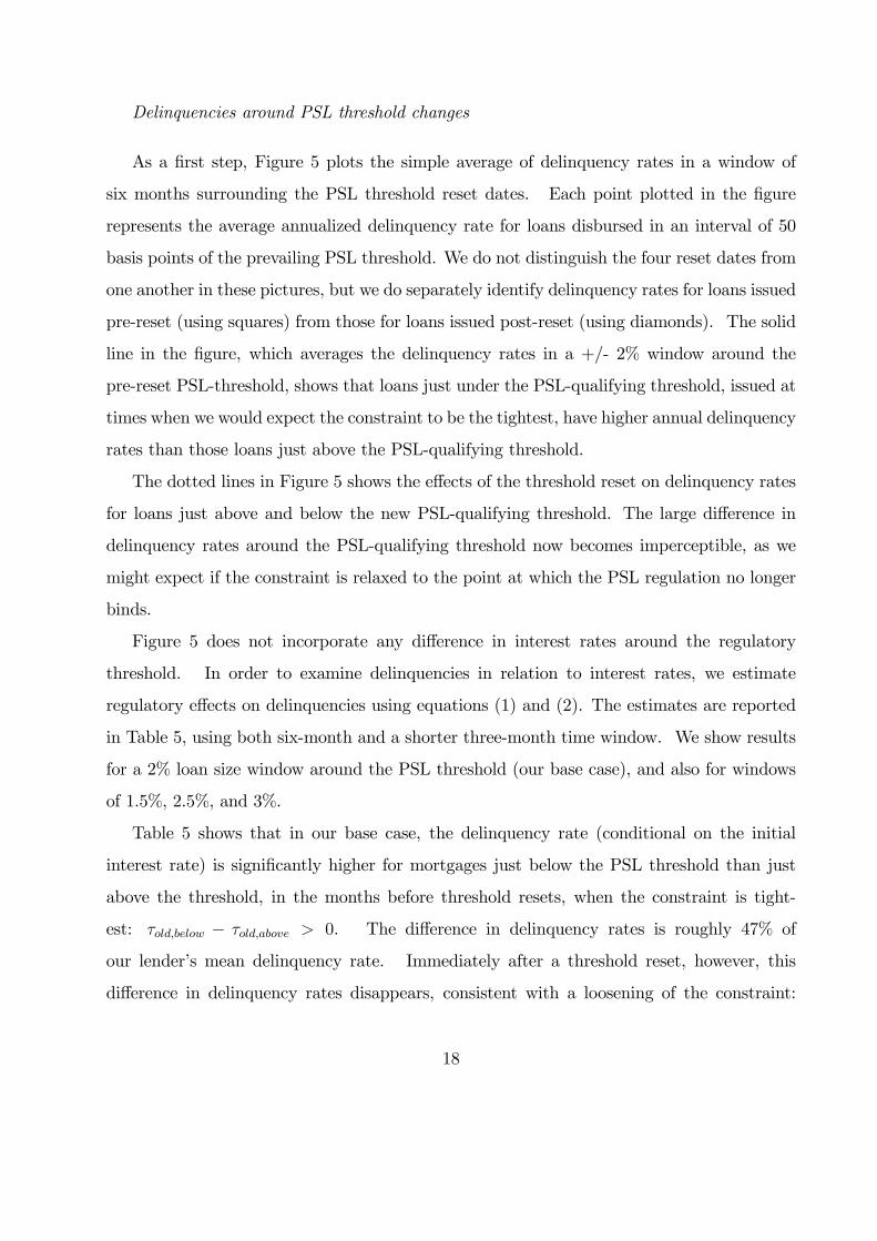
As a first step, Figure 5 plots the simple average of delinquency rates in a window of

six months surrounding the PSL threshold reset dates. Each point plotted in the figure

represents the average annualized delinquency rate for loans disbursed in an interval of 50

basis points of the prevailing PSL threshold. We do not distinguish the four reset dates from

one another in these pictures, but we do separately identify delinquency rates for loans issued

pre-reset (using squares) from those for loans issued post-reset (using diamonds). The solid

line in the figure, which averages the delinquency rates in a +/- 2% window around the

pre-reset PSL-threshold, shows that loans just under the PSL-qualifying threshold, issued at

times when we would expect the constraint to be the tightest, have higher annual delinquency

rates than those loans just above the PSL-qualifying threshold.

The dotted lines in Figure 5 shows the effects of the threshold reset on delinquency rates

for loans just above and below the new PSL-qualifying threshold. The large difference in

delinquency rates around the PSL-qualifying threshold now becomes imperceptible, as we

might expect if the constraint is relaxed to the point at which the PSL regulation no longer

binds.

Figure 5 does not incorporate any difference in interest rates around the regulatory

threshold. In order to examine delinquencies in relation to interest rates, we estimate

regulatory effects on delinquencies using equations (1) and (2). The estimates are reported

in Table 5, using both six-month and a shorter three-month time window. We show results

for a 2% loan size window around the PSL threshold (our base case), and also for windows

of 1.5%, 2.5%, and 3%.

Table 5 shows that in our base case, the delinquency rate (conditional on the initial

interest rate) is significantly higher for mortgages just below the PSL threshold than just

above the threshold, in the months before threshold resets, when the constraint is tight-

est: τold,below − τold,above > 0. The difference in delinquency rates is roughly 47% of

our lender’s mean delinquency rate. Immediately after a threshold reset, however, this

difference in delinquency rates disappears, consistent with a loosening of the constraint:

18

τold,below − τold,above ≈ 0. As a result, the difference in difference is significantly positive:

(τold,below − τold,above)− (τnew,below − τnew,above) > 0.

Controlling for disbursal cohort, in the period immediately before a PSL threshold reset,

interest rates at issuance for loans just below the PSL threshold are 69 basis points on

average higher than on loans just above the threshold. However, this difference in initial

interest rates can only explain roughly 20% of the observed difference in delinquency rates

around the threshold. The remaining 80% is the effect we estimate above.

While these results are not particularly sensitive to the size of the time window around

the date of the PSL threshold resets, our results do weaken as we include loans further away

from the PSL-qualifying threshold. Disbursed loans of sizes infinitesimally greater than the

PSL threshold have very low delinquency rates, perhaps because the lender is only willing to

make such loans to especially reliable borrowers, without forcing the borrower into a slightly

smaller PSL-qualifying loan, despite the obvious incentives to do so. In contrast, loans two

to three percent above the PSL threshold experience delinquency rates which are closer to

the average, tempering estimates as these loans enter the sample.

In the appendix we report estimates of a linear model, estimated using NLLS or OLS

and a 2% loan size window. These estimates are broadly consistent with those for the Cox

proportional hazard model reported in Table 5.

An alternative specification

As an alternative approach, using the same sample of loans, we replace the discrete

treatment dummies with a variable PSLTightnessi. This variable proxies for the intensity

of the pressure faced by the lender at loan disbursal under the assumption that PSL threshold

levels are reset to just relax the prevailing constraint.8 Specifically, during the three or six-

month periods prior to the threshold resets, for PSL-qualifying loans, we set PSLTightnessi

equal to the natural logarithm of the ratio of the new nominal PSL threshold to the old

8As before, we restrict the sample to the short window around the reset dates, and to loans just aboveand below the threshold, to generate maximal comparability between loans being compared in the usualRDD fashion.

19

nominal PSL threshold. The variable takes the value of zero for loans disbursed after the

threshold resets or above the PSL threshold.

We model:

Pr[δi,t] = Zt−1exp(αc + βri + ηPSLTightnessi) + ei,t. (4)

When PSLTightness is higher at the time of disbursing loan i, we expect that the PSL

norm is more diffi cult to meet, consequently raising pressure on the lender to make lower-

quality loans. We therefore expect η > 0. Panel B of Table 5 shows that this approach does

not yield significant results, perhaps owing to noise in the construction of our PSLTightness

proxy.

3.2 Regulation and Delinquencies: Risk Weights

We now turn to analyzing the impact of risk-weight regulations on loan delinquency rates.

In the early part of our sample, all mortgage loans had the same risk weights in India,

100 percent of the issued amount. In early 2002, the Reserve Bank of India decreased risk

weights, and hence capital requirements, on loans with LTV ratios of 75 percent or lower.

Subsequently, the risk weights on these less leveraged loans fluctuated between 50 or 75

percent.9

We test the hypothesis that the impact of these regulatory changes is to change incentives

for lending at different LTV ratios, and hence, to affect delinquency rates on loans issued

at these different LTV levels, conditional on initial interest rates. As an illustration, in

April 2002, each rupee of bank capital would allow the lending of 12.5 rupees to high and

low LTV borrowers given the provisioning requirements against 100% risk weights. As a

consequence, we expect that the interest-rate-adjusted delinquency rates on loans to the two

types of borrowers should be similar for loans issued during this period. However following

the regulatory change, in June 2002, a rupee of capital allows a bank to lend 25 rupees to

9The Reserve Bank of India also applied larger risk weights to mortgage loans above 75 lakh rupees.However, we have very few mortgage loans this large in the sample, and are therefore unable to drawinferences from this source of variation.

20

any borrower who wishes to borrow at an LTV ratio of 75% or lower. All else equal, holding

the less leveraged loans now allows for a greater return on the bank’s capital. The same

story applies to housing finance companies, with slightly adjusted dates and risk weights

(see Figure 3). We expect financial institutions to respond to this regulatory incentive by

extending greater amounts of credit to lower leverage loans following downward adjustments

in their risk weights, with a concomitant increase in excess delinquencies observed on these

lower leverage loans.

To begin with, we plot the simple average of delinquency rates in a window of six months

surrounding the dates on which risk-weights on less-leveraged loans change. In Figure 6, each

plotted point represents the average annualized delinquency rate for loans disbursed at each

percentage point loan-cost ratio shown on the horizontal axis. Again, we do not distinguish

the individual change dates from one another in these pictures. We do, however, separately

average delinquency rates for loans issued when the difference between risk-weights on highly

leveraged and less-leveraged loans is relatively low, at 0 or 25% (represented by diamonds),

from those issued when the difference in risk-weights is substantial, at 50% (squares).

The solid line in the figure, which averages the delinquency rates in a +/- 2% window

around the loan-cost ratio qualifying threshold, shows that loans just under this threshold,

issued when risk weights significantly favour less leveraged loans, are slightly more likely

to be delinquent than loans with slightly higher leverage, immediately above the regulatory

threshold. This is a striking result because delinquencies normally increase with the LTV

ratio (see for example Campbell and Cocco 2014). The dotted line in Figure 6 shows that

when the difference in risk weights is either zero or small, the delinquency rate is indeed

slightly higher for more highly leveraged loans as one would normally expect. As in Figure

5, these results do not control for the initial interest rates on loans.

Next, we adapt the framework outlined in equation (1) to compare delinquencies on loans

disbursed just below/at and just above a 75 percent loan-to-cost ratio (which we measure

at loan disbursal), just before and after the upward or downward adjustment of the risk

weights on less leveraged loans, while controlling for initial interest rates. When the risk

weights on less leveraged loans are adjusted downwards, we denote those disbursed before

21

the adjustment (when risk weights are relatively close together) with the subscript close, and

denote those disbursed after the risk weight adjustment (when risk weights are further apart)

with the subscript far. When the risk weights on less leveraged loans are adjusted upwards,

we denote those disbursed before the adjustment (when risk weights are relatively far apart)

with the subscript far, and denote those disbursed after the risk weight adjustment (when

risk weights are closer together) with the superscript close. Thus, to assess the impacts of

the risk-weight changes on the delinquency rates of loans with different LTVs we model τ ′Di

in equation (1) as:

τ ′Di = τclose,belowDi,close,below + τclose,aboveDi,close,above

+ τfar,belowDi,far,below + τfar,aboveDi,far,above, (5)

where Di,close,below is a dummy variable for loans with a loan-to-cost ratio ≤ 0.75, issued when

the risk weights across loans of varying leverage are closer together; Di,close,above is a dummy

variable for loans with a loan-to-cost ratio > 0.75, issued when the risk weights across loans

of varying leverage are closer together; Di,far,below is a dummy variable for loans with a loan-

to-cost ratio ≤ 0.75, issued when the risk weights across loans of varying leverage are further

apart; and Di,far,above is a dummy variable for loans with a loan-to-cost ratio > 0.75, issued

when the risk weights across loans of varying leverage are further apart.

Following the reasoning described above, we expect that

τfar,below − τfar,above > (τfar,below − τfar,above)− (τclose,below − τclose,above) ≥ 0. (6)

We test both these inequalities below.

Delinquencies around risk weight changes

We estimate risk-weight effects on delinquencies using equations (1) and (5). The es-

timates are reported in Table 6, using both six and three-month time windows. We show

22

results for a 2% leverage ratio window around the risk weight threshold (our base case),

and also for windows of 1% and 3%.

We find some evidence in support of the inequalities in equation (6). Our estimates

of τfar,below − τfar,above and (τfar,below − τfar,above)− (τclose,below − τclose,above) are almost always

positive. However, the null hypotheses that these differences are zero can only be rejected

when we use a narrow three-month time window and a leverage ratio window of 1% or 2%.

A continuous approach

Here, we assume that the interest-rate-adjusted difference in delinquencies on loans with

just above and below 75 percent loan-cost is proportional to the difference in risk weights

on these mortgages. Specifically, we construct RiskWeightAdvantagei as the amount by

which the risk weight prevailing at the time of loan i’s disbursal falls below the 100% risk

weight on more highly levered loans. For less levered loans, RiskWeightAdvantagei varies

between zero and 0.5, and for loans with LTV > 75%, this variable takes the value of zero.

We then estimate

Pr[δi,t] = Zt−1exp(αc + βri + ηRiskWeightAdvantagei) + ei,t. (7)

Panel B of Table 6 shows that when we estimate this model we almost always find η > 0

as expected. The coeffi cient estimates are always statistically significant when we use a

three-month time window around the changes in risk weights. The three-month estimate

for the base case with a 2% leverage window imply that the largest advantage in risk weights

given to less leveraged mortgages resulted in increased delinquencies of these mortgages by

roughly 30% of the population average delinquency rate (risk weight advantage of 0.5 times

a coeffi cient of 0.59).

23

4 Reclassification of Non-Performing Assets

In this section we examine another regulatory change that took place during our sample

period. On March 31, 2004 for banks, and March 31, 2005 for HFCs, the classification of

“non-performing assets”(or NPAs) was changed to 90 days past due from the previous time

period of 180 days past due. This regulatory reclassification of 90-day delinquencies, and its

implications for provisioning requirements, may have contributed to the sharp decline in 90-

day delinquency rates seen in Figure 4. One mechanism by which this might occur is that

the reclassification may have given our mortgage lender the incentive to more intensively

monitor shorter-term delinquencies (say 30 days past due), and to take earlier action to

forestall 90-day delinquency.

To evaluate this, we look at the expected loss given shorter-term delinquency before and

after our lender adopted the regulatory reclassification, which was a short time before it was

offi cially mandatory (March 2004 for banks, April 2005 for housing finance companies).10

Expected loss is the product of the probability of experiencing a longer-term delinquency

and the loss given longer-term delinquency. Table 7 looks at the first of these two elements,

computing transition probabilities of loans that hit the 30-day delinquency threshold to the

90-day delinquency mark, as well as the transition probability of 90-day delinquencies to the

180-day delinquent mark.

The table shows that across the entire sample period, 22.7% (22.8%) of 30-day (90-

day) delinquent loans eventually become 90 days (180 days) delinquent. However, in the

period prior to our lender’s adoption of the NPA reclassification, the 30 to 90 day delinquent

transition probability was 29.2%, almost twice the post-adoption transition probability of

16.0%. The reduction, of 13.3% is highly statistically significant. The lender may have

substantially reduced this transition probability by exerting effort to pursue borrowers more

aggressively to avoid the build up of non-performing assets. The 90-day to 180-day transition

10While we are unable to identify the precise date when the lender adopted the regulation in the interests ofpreserving anonymity, this occurred not too distant from when the change in regulation became mandatoryfor banks. It does not make much difference to our results when we use the offi cial date rather than thedate at which the lender implemented the change internally.

24

probability falls by a negligible 1.3% following the adoption of the reclassification. This

suggests there are relatively fewer incentives to take action in the post adoption period

once the loan has already been classified as a non-performing asset (and as the 180 day

definition looms in the pre-adoption period). Another possibility is that loans past the 90-

day delinquency mark are simply very diffi cult to collect on despite the lender’s exertions.11

To better understand the magnitude of loss given delinquency, we acquire a sample

of 10,000 loans from the total population of loans. As our focus is to understand the

determinants of mortgage risk, we randomly sample 2,500 fixed-rate and 2,500 variable-

rate loans from the set of 90-day delinquent loans, and a further 2,500 fixed-rate and 2,500

variable-rate loans from the set of loans that do not experience a 90-day delinquency. In

each sub-sample of 2,500 loans, we further ensure that we sample an equal number (1,250)

from the early period in the data (disbursed prior to January 2000) and the later period

(disbursed between January 2000 and December 2004). We have verified that this 10,000

loan sample has statistically indistinguishable characteristics from the population of loans

from which we draw. For each one of these 10,000 loans, we are able to track the full payment

history over time, as well as deviations from contracted repayments. We can compute the

latter as we are also given the equated monthly installment (EMI) for each of these loans in

each month, which is the expected monthly principal repayment plus interest amount. We

ensure that we weight any measures constructed using this sample, so that they are reflective

of the larger population of loans from which the sampling occurred.

For each loan in the sample, we construct a measure of losses accrued over time. To do

so, we accumulate payments and EMI over time, and compute the “cumulative installment

deficit”(or CID) as Min(0, cumulative payment-cumulative EMI)/EMI. This measure takes

the value of zero if monthly payments exceed or equal the EMI, and is negative otherwise,

indicating when borrowers are in arrears. The cumulation ensures that if overpayments are

11The 2002 implementation of SARFAESI, described above, allowed for easier restructuring and reposses-sion of delinquent loans. However the small change in the 90-180 day transition probability despite thisregulatory change mirrors the insignificant post-SARFAESI change in the ∆CID debt collection rate that wedefine and analyze below. These results suggest that at least for housing loans, this particular regulatorychange may not have had very large effects.

25

made to redress arrears, these are allowed to push the measure towards zero. The division

by EMI puts the cumulative installment deficit into units of required monthly payments.

Figure 7 plots the CID measure around 30-day delinquencies, before and after our lender

adopted the reclassification of NPAs. The measure is cross-sectionally demeaned by both

cohort-year and calendar-year, to ensure that we are not picking up cohort or macroeconomic

effects. In both panels of Figure 7, date 0 is the first date that the loan is declared 30-days

delinquent (values below 1 are possible because of the cross-sectional demeaning). The top

panel shows that prior to the change in the regulatory definition of NPAs, loans declared

30-days delinquent on average inflicted a cost on the mortgage provider of roughly 1.1 EMIs

after a year. Post-March 2004, there is a substantial recovery in this number, with such

30-delinquent loans roughly 0.4 EMIs delinquent 12 months later. The bottom panel of the

figure shows that this change in the behavior of the CID after the regulatory redefinition of

NPAs is highly statistically significant.

We undertake this analysis more formally by estimating how changes in the CID vary

following a 30-day delinquency, but prior to hitting the 90-day threshold, both before and

after the regulatory redefinition of the NPA period. To do so, we estimate expected debt

collection rates– changes in the CID– as a polynomial function of the level of the CID prior

to the 90-day delinquency mark (i.e., a CID level of −3), allowing for a jump in the rate at

the 90-day delinquency mark, and modelled as a linear function of the CID beyond the 90-

day delinquency mark. As before, we include time- and cohort-specific fixed effects during

estimation to ensure that we are not merely picking up some of the broader changes detected

earlier in the regulatory and macroeconomic environment.

Figure 8 shows how the estimated debt collection rate varies before and after the 90-day

delinquency threshold, before and after the regulatory reclassification of NPAs was adopted.

The figure reveals that following the adoption of the reclassification, the debt collection

rate prior to hitting the 90-day mark increased substantially relative to the pre-adoption

period, with a significant discontinuity at the 90-day threshold, where the debt collection

rate falls sharply.12 We also consider whether the introduction of SARFAESI had any

12The increase in the debt collection rate prior to the 90-day delinquency mark, and the discontinuity

26

significant impacts on the ability to collect on debts, and find that differences are minimal

and statistically insignificant.

While these changes to debt collection rates are evident in the data, one potential inter-

pretation is that the redefinition of NPAs from 180 to 90 days simply shifted the inevitable

recovery of cash from delinquent borrowers by the 90-day difference between these two dates.

In other words, perhaps the change merely provided a time-value improvement in the net

cash flows of the mortgage provider, but no more substantial impacts.

To address this question, Figure 9 shows the cumulative distribution function (CDF) of

the change in the CID (time- and cohort-demeaned) in the year following the first 30 day

delinquency. This CDF is plotted for three time periods, namely, January 1995 to June

2002, when SARFAESI was first implemented; July 2002 to the date our lender adopted a

reclassification of NPAs; and from this adoption date until the end of the sample period in

2010. We plot the figure on a log scale to focus attention on the very worst cases (i.e., those

loans with the greatest degradation in CID over the year following the date of first 30-day

delinquency), as these loans are the most likely candidates for a complete write-off.

The figure shows that the post-NPA redefinition CDF first-order stochastically dominates

both the pre- and post-SARFAESI CDFs, showing a substantial reduction in the incidence

of high degradation in the CID. While SARFAESI appears to have had some beneficial

impacts for the very worst cases, this is dwarfed by the large impact of the NPA redefinition.

These substantial impacts on eventual bad debts of this regulatory redefinition are striking,

as it appears that there are important benefits to incentivizing mortgage providers to detect

and take early action on delinquencies.

In Figure 10 we document some evidence that the change in the regulatory classification

of NPAs affected screening at mortgage origination as well as mortgage monitoring practices.

This figure reports the same curve as in Figure 9, separately for loans originated in six-month

windows before and after the NPA reclassification was adopted by our lender. The left tail

at that mark are both economically and statistically significant. The online empirical appendix plots thedifference between the pre- and post-adoption debt collection rates with associated bootstrap confidenceintervals.

27

of the distribution is noticeably thicker for loans originated before the reclassification. Since

we are observing delinquency experiences for both cohorts of loans over the same post-

reclassification period (with presumably enhanced monitoring), the reduced probability of

very bad outcomes for loans issued post-adoption is evidence that mortgage screening at

origination was heightened as well.

In summary, a simple change in the regulatory definition of NPAs appears to have signif-

icantly moderated mortgage delinquencies. The impacts are visible in both the probability

of delinquency and the eventual loss given delinquency.

A natural question that arises here is why the lender did not implement such changes

to monitoring voluntarily, earlier than the regulatory imposition of the change, given the

significant impacts on short- and long-term delinquency rates. The issue here is that loan

screening and monitoring are costly, and we do not measure the costs. Given that we do

not (and cannot feasibly) assess these costs, we are unable to assess the net impact on the

lender of implementing quicker action on potentially delinquent loans, despite documenting

that the benefits of such monitoring are large. It is also possible that tougher screening, by

reducing credit extended to lower quality borrowers, conflicts with the lender’s incentives to

lend to the priority sector and may incur political or public relations costs.

5 Conclusion

The Indian regulatory and macroeconomic environment has changed dramatically during

the last two decades. A fast-developing housing finance system has coped with significant

variation in default rates and interest rates, and regulatory changes in the incentives to

originate mortgages in general, and small loans in particular. In this paper we have explored

the effects of such regulatory changes on mortgage risk using an empirical strategy that

links time variation in regulation with expected cross-sectional impacts on different types of

mortgages.

We have presented evidence that regulatory subsidies for low-cost housing and less lever-

aged loans are associated with higher delinquencies, controlling for interest rates at loan

28

issuance, and that changes to the definition of non-performing assets impacted behavior in

response to early evidence of payment delinquencies. While it is diffi cult to generalize find-

ings from one country, or to make welfare statements in the absence of a full estimation of

both costs and benefits, our findings on the infrequent adjustment of PSL-thresholds suggest

that paying attention to the design of policies may yield rewards, and the estimated effect of

the regulatory redefinition of NPAs suggests that even seemingly minor regulatory changes

can have important impacts on mortgage monitoring and origination practices, and hence

on mortgage risk.

29

References

Acharya, Viral V., Matthew Richardson, Stijn van Nieuwerburgh, and Lawrence J. White,

2011, Guaranteed to Fail: Fannie Mae, Freddie Mac, and the Debacle of Mortgage

Finance, Princeton University Press, Princeton, NJ.

Adelino, Manuel, Kristopher Gerardi, and Paul S. Willen, 2013, “Why Don’t Lenders Rene-

gotiate More Home Mortgages? Redefaults, Self-Cures, and Securitization”, Journal

of Monetary Economics 60, 835—853.

Adelino, Manuel, Antoinette Schoar, and Felipe Severino, 2014, “Credit Supply and House

Prices: Evidence from Mortgage Market Segmentation”, unpublished paper, Duke

University and MIT.

Agarwal, Sumit, Gene Amromin, Itzhak Ben-David, Souphala Chomsisengphet, and Dou-

glas D. Evanoff, 2011, “The Role of Securitization in Mortgage Renegotiation”, Journal

of Financial Economics 102, 559—578.

Agarwal, Sumit, Efraim Benmelech, Nittai Bergman, and Amit Seru, 2012, “Did the Com-

munity Reinvestment Act (CRA) Lead to Risky Lending?”, NBERWorking Paper No.

18609.

Aghion, Philippe, Robin Burgess, Stephen J. Redding, and Fabrizio Zilibotti, 2008, “The

Unequal Effects of Liberalization: Evidence from Dismantling the License Raj in In-

dia”, American Economic Review, 98(4), 1397—1412.

Amromin, Gene, Jennifer Huang, Clemens Sialm, and Edward Zhong, 2011, “Complex

Mortgages,”NBER Working Paper No. 17315.

Anagol, Santosh, and Hugh Kim, 2012, “The Impact of Shrouded Fees: Evidence from a

Natural Experiment in the Indian Mutual Funds Market”, American Economic Review,

102(1), 576-593.

30

Avery, Robert, and Ken Brevoort, 2011, “The Subprime Crisis: Is Government Housing

Policy to Blame?,”FEDS Working Paper 2011-36, Federal Reserve Board.

Baily, Martin N., 2011, ed., The Future of Housing Finance: Restructuring the U.S. Resi-

dential Mortgage Market, Brookings Institution Press, Washington, DC.

Balasubramanyan, Lakshmi, and Kevin Jacques, 2011, “Risk Weights in Regulatory Capital

Standards: Is it Necessary to ‘Get It Right’?,”Networks Financial Institute Working

Paper No. 2011-23.

Banerjee, Abhijeet, Shawn Cole, Esther Duflo, and Leigh Linden, 2007, “Remedying Edu-

cation: Evidence from Two Randomized Experiments in India,”Quarterly Journal of

Economics, 122(3), 1235-1264.

Besley, Tim, and Robin Burgess, 2000, “Land Reform, Poverty Reduction and Growth:

Evidence from India”, Quarterly Journal of Economics 115, 389-430.

Bhutta, Neil, Jane Dokko, and Hui Shan, 2010, “The Depth of Negative Equity and Mort-

gage Default Decisions,”FEDS Working Paper 2010-35, Federal Reserve Board.

Calem, Paul, and James Follain, 2007, “Regulatory Capital Arbitrage and the Potential

Competitive Impact of Basel II in the Market for Residential Mortgages”, Journal of

Real Estate Finance and Economics 35, 197—219.

Campbell, John Y., 2013, “Mortgage Market Design”, Review of Finance 17, 1—33.

Campbell, John Y. and Joao F. Cocco, 2014, “A Model of Mortgage Default”, forthcoming

Journal of Finance.

Campbell, John Y., Stefano Giglio, and Parag Pathak, 2011, “Forced Sales and House

Prices”, American Economic Review 101, 2108—2131.

Campbell, John Y., Tarun Ramadorai, and Vimal Balasubramaniam, 2014, “Prudential

Regulation of Housing Finance in India 1995-2011”, regulatory appendix, available at:

http://intranet.sbs.ox.ac.uk/tarun_ramadorai/TarunPapers/PrudentialRegulationAppendix.pdf.

31

Campbell, John Y., Tarun Ramadorai, and Benjamin Ranish, 2014, “Appendix to Camp-

bell, Ramadorai, and Ranish”, empirical appendix, available at:

http://intranet.sbs.ox.ac.uk/tarun_ramadorai/TarunPapers/MortgageEmpiricalAppendix.pdf.

Campbell, Tim S. and J. Kimball Dietrich, 1983, “The Determinants of Default on Insured

Conventional Residential Mortgage Loans”, Journal of Finance 38, 1569—1581.

Canner, Glenn and Wayne Passmore, 1997, “The Community Reinvestment Act and the

Profitability of Mortgage-Oriented Banks”, unpublished paper, Federal Reserve Board.

Cole, Shawn A., 2009, “Fixing Market Failures or Fixing Elections? Elections, Banks and

Agricultural Lending in India”, American Economic Journal: Applied Economics 1,

219—50.

Cox, David R., 1972, “Regression Models and Life Tables”, Journal of the Royal Statistical

Society B, 34, 187—220.

Dahl, Drew, Douglass Evanoff, and Michael Spivey, 2000, “Does the Community Reinvest-

ment Act Influence Lending? An Analysis of Changes in Bank Low-Income Mortgage

Activity,”Working Paper No. 2000-06, Federal Reserve Bank of Chicago

DeFusco, Anthony, and Andrew Paciorek, 2014, “The Interest Rate Elasticity of Mortgage

Demand: Evidence from Bunching at the Conforming Loan Limit”, FEDS Working

Paper 2014-11, Federal Reserve Board.

Demyanyk, Yuliya, and Otto van Hemert, 2011, “Understanding the Subprime Mortgage

Crisis”, Review of Financial Studies 24, 1848—1880.

Duca, John V. and Stuart S. Rosenthal, 1994, “Do Mortgage Rates Vary Based on House-

hold Default Characteristics? Evidence Based on Rate Sorting and Credit Rationing”,

Journal of Real Estate Finance and Economics 8, 99—113.

Ellis, Luci, 2008, “The Housing Meltdown: Why Did It Happen in the United States?”,

Bank for International Settlements Working Paper 259.

32

Foote, Christopher, Kristopher Gerardi, Lorenz Goette, and Paul Willen, 2010, “Reducing

Foreclosures: No Easy Answers,”NBER Macroeconomics Annual 2009, 89—138.

Hunt, Stefan, 2010, “Informed Traders and Convergence to Market Effi ciency: Evidence

from a New Commodity Futures Exchange”, unpublished paper, Harvard University.

International Monetary Fund, 2011, “Housing Finance and Financial Stability– Back to

Basics?”, Chapter 3 inGlobal Financial Stability Report, April 2011: Durable Financial

Stability– Getting There from Here, International Monetary Fund, Washington, DC.

Johnson, Kathleen W. and Geng Li, 2011, “Are Adjustable-Rate Mortgage Borrowers Bor-

rowing Constrained?”, forthcoming Real Estate Economics.

Kashyap, Anil, Raghuram Rajan, and Jeremy Stein, 2008,“Rethinking Capital Regulation”,

in Federal Reserve Bank of Kansas City Symposium on Maintaining Stability in a

Changing Financial System, 431-471.

Keys, Benjamin, Tanmoy Mukherjee, Amit Seru, and Vikrant Vig, 2010, “Did Securitiza-

tion Lead to Lax Screening? Evidence from Subprime Loans”, Quarterly Journal of

Economics 125, 307—362.

Kroszner, Randall, 2008, “The Community Reinvestment Act and the Recent Mortgage

Crisis,”speech at the Confronting Concentrated Poverty Policy Forum.

von Lilienfeld-Toal, Dilip Mookherjee and Sujata Visaria, 2012, “The Distributive Impact

of Reforms in Credit Enforcement: Evidence from Indian Debt Recovery Tribunals”,

Econometrica, 89, 497-558.

Melzer, Brian T., 2011, “Mortgage Debt Overhang: Reduced Investment by Homeowners

with Negative Equity”, unpublished paper, Northwestern University.

Mian, Atif and Amir Sufi, 2009, “The Consequences of Mortgage Credit Expansion: Evi-

dence from the U.S. Mortgage Default Crisis”, Quarterly Journal of Economics 124,

1449—1496.

33

Piskorski, Tomasz, Amit Seru, and Vikrant Vig, 2011, “Securitization and Distressed Loan

Renegotiation: Evidence from the Subprime Mortgage Crisis”, Journal of Financial

Economics 97, 369—397.

Tiwari, Piyush and Pradeep Debata, 2008, “Mortgage Market in India”, Chapter 2 in

Danny Ben-Shahar, Charles Ka Yui Leung, and Seow Eng Ong eds. Mortgage Markets

Worldwide, Blackwell.

U.S. Treasury and Department of Housing and Urban Development, 2011, Reforming Amer-

ica’s Housing Market: A Report to Congress, Washington, DC.

Verma, R.V., 2012, “Evolution of the Indian Housing Finance System and Housing Market”,

Chapter 14 in Ashok Bardhan, Robert H. Edelstein, and Cynthia A. Kroll eds. Global

Housing Markets: Crises, Policies, and Institutions, John Wiley.

Vig, V., 2013, “Access to Collateral and Corporate Debt Structure: Evidence from a Natural

Experiment,”Journal of Finance, 68, 881—928.

Wooldridge, Jeffrey M., 2002, Econometric Analysis of Cross Section and Panel Data, MIT

Press, Cambridge, MA.

34

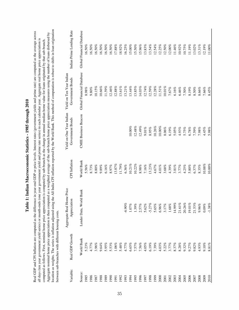
Var

iab

le:

Rea

l G

DP

Gro

wth

Aggre

gat

e R

eal

Ho

me

Pri

ce

Ap

pre

ciat

ion

CP

I In

flat

ion

Yie

ld o

n O

ne

Yea

r In

dia

n

Go

ver

nm

ent

Bo

nd

s

Yie

ld o

n T

en Y

ear

Ind

ian

Go

ver

nm

ent

Bo

nd

sIn

dia

n P

rim

e L

end

ing R

ate

So

urc

e:W

orl

d B

ank

Len

der

Dat

a, W

orl

d B

ank

Wo

rld

Ban

kC

MIE

Busi

nes

s B

eaco

nG

lob

al F

inan

cial

Dat

abas

eG

lob

al F

inan

cial

Dat

abas

e

19

85

5.2

3%

5.5

6%

8.9

8%

16

.50

%

19

86

4.7

7%

8.7

3%

9.8

0%

16

.50

%

19

87

3.9

6%

8.8

0%

10

.15

%1

6.5

0%

19

88

9.6

4%

9.8

9%

10

.66

%1

6.5

0%

19

89

5.9

5%

6.1

6%

11

.59

%1

6.5

0%

19

90

5.5

3%

8.9

7%

12

.46

%1

6.5

0%

19

91

1.0

6%

13

.87

%1

2.8

8%

17

.88

%

19

92

5.4

8%

11

.79

%1

3.6

1%

18

.92

%

19

93

4.7

7%

-6.9

0%

6.3

6%

13

.21

%1

6.2

5%

19

94

6.6

5%

1.0

7%

10

.21

%1

0.0

0%

13

.44

%1

5.0

0%

19

95

7.5

7%

1.3

9%

10

.22

%1

2.4

8%

13

.85

%1

5.5

0%

19

96

7.5

6%

2.5

7%

8.9

8%

12

.49

%1

4.0

3%

15

.96

%

19

97

4.0

5%

5.6

2%

7.1

6%

9.0

1%

12

.74

%1

3.8

3%

19

98

6.1

9%

-5.2

7%

13

.23

%8

.95

%1

2.5

9%

13

.54

%

19

99

7.3

9%

5.6

5%

4.6

7%

10

.26

%1

2.2

8%

12

.54

%

20

00

4.0

3%

6.9

6%

4.0

1%

10

.00

%1

1.5

1%

12

.25

%

20

01

5.2

2%

3.1

7%

3.6

8%

8.0

6%

10

.01

%1

2.5

0%

20

02

3.7

7%

1.6

8%

4.3

9%

6.1

9%

7.6

7%

12

.00

%

20

03

8.3

7%

14

.99

%3

.81

%5

.05

%6

.16

%1

1.4

6%

20

04

8.2

8%

21

.61

%3

.77

%4

.93

%6

.46

%1

0.9

2%

20

05

9.3

2%

20

.26

%4

.25

%5

.75

%7

.50

%1

0.7

5%

20

06

9.2

7%

19

.01

%5

.80

%6

.78

%8

.19

%1

1.1

9%

20

07

9.8

2%

21

.53

%6

.37

%7

.59

%8

.50

%1

3.0

2%

20

08

4.9

3%

9.9

6%

8.3

5%

7.9

8%

8.6

6%

13

.31

%

20

09

9.1

0%

0.0

9%

10

.88

%4

.45

%7

.66

%1

2.1

9%

20

10

8.8

1%

-1.3

8%

10

.00

%5

.98

%8

.45

%1

1.0

0%

Tab

le 1

: In

dia

n M

acr

oec

on

om

ic S

tati

stic

s -

1985 t

hro

ugh

2010

Rea

l G

DP

and

CP

I In

flat

ion a

re c

om

pute

d a

s th

e d

iffe

rence

in y

ear-

end

GD

P o

r p

rice

lev

els.

Inte

rest

rat

es (

go

ver

nm

ent

yie

lds

and

pri

me

rate

) ar

e co

mp

ute

d a

s th

e av

erag

e ac

ross

all

day

s (t

en y

ear

go

ver

nm

ent

yie

ld s

erie

s) o

r m

onth

-end

s (o

ne

yea

r go

ver

nm

ent

yie

ld a

nd

pri

me

rate

ser

ies)

in e

ach c

alen

dar

yea

r. A

ggre

gat

e re

al h

om

e p

rice

ap

pre

ciat

ion i

s

com

pute

d a

s fo

llo

ws.

Fir

st,

no

min

al h

om

e p

rice

ap

pre

ciat

ion i

s co

mp

ute

d b

y s

ub

-bra

nch

as

the

chan

ge

in a

nnual

med

ian h

om

e val

ue

for

loan

s o

rigin

ated

by t

hat

sub

-bra

nch

.

Aggre

gat

e no

min

al h

om

e p

rice

ap

pre

ciat

ion i

s th

en c

om

pute

d a

s a

wei

ghte

d a

ver

age

of

the

sub

-bra

nch

ho

me

pri

ce a

pp

reci

atio

n m

easu

res

usi

ng t

he

num

ber

of

loan

s d

isb

urs

ed b

y

loca

tio

n a

s w

eights

. T

he

seri

es i

s in

flat

ion a

dju

sted

usi

ng t

he

All

Ind

ia C

PI

infl

atio

n r

epo

rted

by t

he

Wo

rld

Ban

k.

This

met

ho

d o

f co

mp

uta

tio

n i

s ro

bust

to

shif

ts i

n l

oan

ori

gin

atio

n

bet

wee

n s

ub

-bra

nch

es w

ith d

iffe

rent

ho

usi

ng c

ost

s.

35

By C

ount

By V

alue

Var

iab

le R

ate

Fix

ed R

ate

Var

iab

le R

ate

Fix

ed R

ate

19

95

37

.86

%4

2.9

8%

74

.06

%7

6.0

7%

78

.16

%8

0.9

0%

19

96

47

.45

%5

1.7

8%

68

.77

%6

9.3

8%

77

.60

%8

0.7

4%

19

97

55

.29

%6

0.8

4%

66

.83

%6

8.3

0%

75

.79

%8

0.3

6%

19

98

59

.04

%6

6.7

8%

79

.15

%8

4.5

9%

69

.83

%7

5.0

8%

19

99

65

.55

%7

1.3

2%

80

.62

%8

5.7

1%

63

.55

%6

8.4

3%

20

00

75

.70

%8

1.6

5%

87

.12

%9

1.6

4%

55

.58

%5

8.5

6%

20

01

75

.32

%8

2.3

1%

83

.07

%8

9.5

7%

50

.61

%5

6.7

1%

20

02

84

.40

%8

9.8

3%

78

.88

%9

0.6

7%

44

.42

%5

7.1

6%

20

03

94

.14

%9

4.1

6%

71

.21

%6

9.3

4%

39

.30

%4

7.8

7%

20

04

84

.51

%7

9.9

7%

67

.95

%5

1.6

7%

36

.37

%3

5.4

1%

20

05

90

.40

%9

2.0

9%

64

.69

%7

6.8

1%

33

.03

%3

8.9

6%

20

06

90

.44

%9

2.8

7%

46

.06

%6

7.5

6%

34

.06

%4

1.7

3%

20

07

95

.76

%9

7.7

2%

43

.03

%6

7.0

3%

34

.66

%4

6.3

9%

20

08

99

.44

%9

9.8

0%

42

.73

%3

7.2

9%

20

09

99

.87

%9

9.9

7%

38

.30

%3

9.6

6%

20

10

99

.97

%9

9.9

9%

36

.45

%3

5.7

4%

Shar

e o

f L

oan

Dis

burs

als

Mee

ting R

egula

tio

n R

elev

ant

Thre

sho

lds

Lo

an

-Co

st R

ati

os ≤

75

%

Tab

le 2

: L

evel

an

d V

ari

ati

on

in

Loan

Dis

bu

rsal

Sh

are

Mee

tin

g R

egu

lati

on

Rel

evan

t T

hre

shold

s

Bel

ow

PS

L T

hre

sho

ldV

aria

ble

Rat

e S

har

e o

f D

isb

urs

als

Lo

an d

isb

urs

als

bel

ow

the

PS

L t

hre

sho

ld a

nd

bel

ow

(o

r at

) a

loan

-co

st r

atio

of

75

% a

re g

iven

as

the

shar

e o

f th

e to

tal

val

ue

of

loan

s d

isb

urs

ed i

n t

he

giv

en y

ear.

The

regula

tory

so

urc

e d

ocu

men

ts a

re d

etai

led

in t

he

onli

ne

regula

tory

ap

pen

dix

. S

tati

stic

s fo

r fi

xed

rat

e m

ort

gag

e d

isb

urs

als

afte

r 2

00

7 a

re n

ot

sho

wn d

ue

to

lim

ited

fix

ed r

ate

lend

ing i

n t

hes

e yea

rs.

36

A: Cross-Sectional Means

Variable Fixed Variable Fixed Variable Fixed Variable Fixed Variable Fixed

1995 15.22% 15.00% 13.96 11.66 0.58 0.54 3.73 3.52 1.70% 2.27%

1996 16.39% 16.14% 13.21 10.89 0.57 0.54 3.69 3.45 1.98% 2.56%

1997 15.54% 15.25% 13.18 10.38 0.58 0.55 3.69 3.38 1.76% 2.79%

1998 14.45% 14.09% 13.08 10.06 0.61 0.57 3.67 3.28 1.84% 3.12%

1999 13.58% 13.39% 12.88 10.63 0.64 0.61 3.62 3.31 1.78% 4.38%

2000 12.58% 12.83% 12.95 10.55 0.67 0.67 3.58 3.20 2.13% 4.58%

2001 11.78% 11.76% 12.72 10.23 0.68 0.64 3.56 3.23 2.16% 5.27%

2002 10.92% 10.82% 13.15 10.03 0.70 0.64 3.49 3.21 2.53% 4.63%

2003 10.68% 9.41% 12.88 12.76 0.72 0.65 3.45 3.54 2.36% 2.20%

2004 10.82% 8.13% 14.07 15.13 0.73 0.71 3.65 3.75 2.18% 0.91%

2005 10.42% 8.83% 15.16 15.17 0.74 0.69 3.75 3.72 1.75% 1.26%

2006 10.85% 10.45% 15.23 15.59 0.73 0.70 3.74 3.69 1.53% 1.12%

2007 11.03% 12.26% 15.03 14.68 0.73 0.68 3.75 3.58 1.18% 1.43%

2008 10.79% 15.38 0.72 3.78

2009 9.51% 14.31 0.71 3.72

2010 8.39% 15.59 0.73 3.84

B: Cross-Sectional Standard Deviations

Variable Fixed Variable Fixed Variable Fixed Variable Fixed

1995 0.94% 1.13% 2.51 4.24 0.18 0.20 0.47 0.71

1996 1.28% 1.53% 2.73 4.26 0.18 0.20 0.49 0.74

1997 0.84% 1.22% 2.72 4.49 0.18 0.20 0.51 0.83

1998 0.71% 1.09% 2.81 4.69 0.18 0.20 0.51 0.86

1999 0.51% 0.77% 3.00 4.52 0.18 0.19 0.52 0.80

2000 1.21% 0.85% 3.61 4.57 0.18 0.19 0.57 0.85

2001 1.06% 0.97% 3.97 4.56 0.18 0.24 0.61 0.83

2002 1.46% 0.92% 4.43 4.63 0.19 0.24 0.70 0.81

2003 2.08% 0.89% 4.85 4.77 0.19 0.26 0.78 0.67

2004 2.04% 0.60% 4.97 4.55 0.18 0.21 0.72 0.59

2005 1.73% 0.48% 4.92 4.52 0.18 0.22 0.68 0.60

2006 1.24% 0.76% 4.95 4.48 0.18 0.22 0.70 0.63

2007 0.67% 1.00% 4.41 4.78 0.18 0.23 0.69 0.71

2008 0.59% 4.57 0.18 0.70

2009 0.77% 5.00 0.18 0.72

2010 0.37% 4.55 0.17 0.64

Table 3: Summary Statistics on Loan Characteristics by Disbursal Year

Loan Term (Years)Initial Interest Rate Loan-Cost Ratio Loan-Income Ratio

Loan Term (Years)Initial Interest Rate Loan-Cost Ratio Loan-Income Ratio Cohort 90-Day Delinquency Rate

This table provides equal-weighted yearly means (Panel A) and standard deviations (Panel B) of important characteristics for the more than 1.2

million mortgage loans disbursed by the lender. Cohort delinquency rates are computed as the annual probability that an outstanding and not-yet-90-

day-delinquent loan experiences a 90 day delinquency. This probability is computed separately for each disbursal-year cohort and calendar year. The

delinquency rate below represents the time-series average across calendar year estimates for each disbursal-year cohort. Statistics for fixed rate

disbursals are removed for the years 2008 through 2010, as fixed rate disbursals account for well under one percent of disbursals (by count or value) in

each of these years. Similarly, cohort 90-day delinquency rate is omitted for loans disbursed after 2007 as these loans have not been around long

enough to reliably estimate a delinquency rate.

37

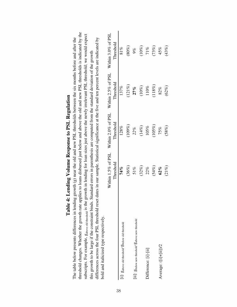
Wit

hin

1.5

% o

f P

SL

Thre

sho

ld

Wit

hin

2.0

% o

f P

SL

Thre

sho

ld

Wit

hin

2.5

% o

f P

SL

Thre

sho

ld

Wit

hin

3.0

% o

f P

SL

Thre

sho

ld

[i]:

gab

ove

old

thre

sho

ld-g

bel

ow

old

thre

sho

ld7

4%

12

8%

13

7%

81

%

(36

%)

(10

9%

)(1

21

%)

(80

%)

[ii]

: g

bel

ow

new

thre

sho

ld-g

abo

ve

new

thre

sho

ld5

1%

22

%2

7%

9%

(32

%)

(14

%)

(10

%)

(10

%)

Dif

fere

nce

: [i

]-[i

i]2

2%

10

5%

11

0%

71

%

(54

%)

(10

5%

)(1

18

%)

(73

%)

Aver

age:

([i

]+[i

i])/

26

2%

75

%8

2%

45

%

(21

%)

(58

%)

(62

%)

(43

%)

Tab

le 4

: L

end

ing V

olu

me

Res

pon

se t

o P

SL

Reg

ula

tion

The

tab

le b

elo

w p

rese

nts

dif

fere

nce

s in

len

din

g g

row

th (

g)

nea

r th

e o

ld a

nd

new

PS

L t

hre

sho

lds

bet

wee

n t

he

six m

onth

s b

efo

re a

nd

aft

er t

he

thre

sho

ld c

han

ges

. W

het

her

the

gro

wth

rat

e ap

pli

es t

o l

oan

s d

isb

urs

ed j

ust

bel

ow

and

ab

ove

the

old

and

new

PS

L t

hre

sho

lds

is i

nd

icat

ed b

y t

he

sub

scri

pts

. F

or

exam

ple

, g

abo

ve

old

thre

sho

ld i

s th

e gro

wth

in l

end

ing f

or

loan

siz

es j

ust

ab

ove

the

new

ly i

rrel

evan

t P

SL

thre

sho

ld;

we

wo

uld

exp

ect

this

gro

wth

to

be

larg

e if

the

const

rain

t b

ind

s. S

tand

ard

err

ors

in p

aren

thes

is a

re c

om

pute

d f

rom

the

stan

dar

d d

evia

tio

n o

f th

e gro

wth

dif

fere

nce

s ac

ross

the

four

PS

L t

hre

sho

ld r

eset

dat

es i

n o

ur

sam

ple

. S

tati

stic

al s

ignif

ican

ce a

t th

e fi

ve

and

ten

per

cent

level

s ar

e in

dic

ated

by

bo

ld a

nd

ita

lici

zed

typ

e re

spec

tivel

y.

38

Loan Size Window: 1.5% 2.0% 2.5% 3.0%

Observations (Above Threshold): 812 1,378 1,810 2,307

Observations (At/Below Threshold): 31,738 32,400 33,086 33,561

Observations (Above Threshold): 398 659 894 1,123

Observations (At/Below Threshold): 16,172 16,481 16,857 17,129

0.57 0.47 0.15 0.07

(0.24) (0.14) (0.20) (0.17)

0.35 -0.07 0.07 0.04

(0.23) (0.19) (0.17) (0.14)

[i]-[ii] 0.22 0.54 0.07 0.03

(0.23) (0.23) (0.30) (0.24)

0.56 0.55 0.29 0.16

(0.33) (0.15) (0.19) (0.21)

0.15 0.02 0.18 0.26

(0.40) (0.32) (0.24) (0.20)

[i]-[ii] 0.41 0.52 0.11 -0.11

(0.39) (0.24) (0.32) (0.32)

η -0.03 -0.02 -0.03 -0.04

(0.17) (0.16) (0.17) (0.16)

η -0.01 0.03 0.05 -0.01

(0.17) (0.18) (0.19) (0.18)

Using a Three-month Time Window Around PSL Threshold Changes

A. Difference-in-Difference Specification (Equation 1)

Using a Six-month Time Window Around PSL Threshold Changes

This table provides parameters of interest from Equations 1 (in section A) and 4 (in section B) in the

paper estimated as Cox hazard models on the population of loans disbursed around priority sector

lending (PSL) thresholds around the time of PSL threshold changes. In section A, the reported

differences represent the impact of PSL qualification on abnormal delinquency rates before [i] and

after [ii] the PSL threshold is raised, relaxing the constraint. In section B, the coefficient η represents

the impact of our proxy for PSL constraint tightness (the natural log of the ratio of new-over-old PSL

thresholds) on abnormal delinquency rates of PSL. Coefficients and standard errors are scaled to

reflect the impact relative to the average delinquency rate in the full loan sample. Standard errors

(reported in parentheses) are computed by bootstrapping years of the panel data, with bold and

italicized type representing statistical significance at the five and ten percent level respectively.

Table 5: Impact of PSL Regulation on Abnormal Delinquency Rate

Using a Three-month Time Window Around PSL Threshold Changes

Using a Six-month Time Window Around PSL Threshold Changes

Using a Six-month Time Window Around PSL Threshold Changes

Using a Three-month Time Window Around PSL Threshold Changes

B. Abnormal Delinquencies as a Function of PSL Constraint Tightness Proxy (Equation 4)

[i]: τ���,����� − τ���,����

[ii]: τ���,����� − τ���,����

[i]: τ���,����� − τ���,����

[ii]: τ���,����� − τ���,����

39

Loan/Cost Ratio Window: 1.0% 2.0% 3.0%

Observations (Above 75% Loan-Cost): 33,673 78,518 122,524

Observations (At/Below 75% Loan-Cost): 96,634 130,412 154,537

Observations (Above 75% Loan-Cost): 16,207 38,508 59,448

Observations (At/Below 75% Loan-Cost): 47,149 63,782 75,622

0.10 0.03 -0.07

(0.06) (0.06) (0.08)

-0.13 -0.12 -0.01

(0.08) (0.07) (0.06)

[i]-[ii] 0.23 0.15 -0.07

(0.09) (0.10) (0.10)

0.35 0.22 0.03

(0.11) (0.09) (0.06)

-0.23 -0.05 -0.01

(0.15) (0.11) (0.09)

[i]-[ii] 0.59 0.26 0.05

(0.13) (0.13) (0.13)

η 0.22 0.10 -0.03

(0.22) (0.19) (0.23)

η 0.59 0.61 0.28

(0.19) (0.11) (0.11)

Using a Three-month Time Window Around Risk Weight Changes

Table 6: Impact of Risk Weight Regulation on Abnormal Delinquency Rate

This table provides parameters of interest from the combination of Equations 1 (in section A) and Equation

8 (in section B) in the paper estimated as Cox hazard models on the population of loans disbursed around a

75% loan-cost ratio around the time of risk weight changes for loans below 75% loan-to-value. In section

A, the reported values are differences in abnormal delinquency rates on loans disbursed below and above a

75% loan-cost ratio under regimes where risk weights on loans disbursed around that threshold are [i]

relatively far and [ii] relatively close. In section B, the coefficient η represents the impact of the risk weight

advantage carried on less leveraged loans (100% minus the risk weight on these loans) on abnormal

delinquency rates. Coefficients and standard errors are scaled to reflect the impact relative to the average

delinquency rate in the full loan sample. Standard errors (reported in parentheses) are computed by

bootstrapping years of the panel data, with bold and italicized type representing statistical significance at

the five and ten percent level respectively.

Using a Six-month Time Window Around Risk Weight Changes

B. Abnormal Delinquencies as a Function of Risk Weight Advantage (Equation 8)

Using a Three-month Time Window Around Risk Weight Changes

A. Difference-in-Difference Specification (Equation 1)

Using a Six-month Time Window Around Risk Weight Changes

Using a Three-month Time Window Around Risk Weight Changes

Using a Six-month Time Window Around Risk Weight Changes

[i]: τ���,��� − τ���,����

[ii]: τ ���,��� − τ ���,����

[i]: τ���,��� − τ���,����

[ii]: τ ���,��� − τ ���,����

40

Month Relative

Probability of 30 day

Delinquency Transitioning to

90 day Delinquency

Probability of 90 day

Delinquency Transitioning to

180 day Delinquency

For Initial Delinquencies Occurring:

All Months (Jan 1996-Dec 2010) 22.7% 22.8%

(0.3%) (0.4%)

Lender Under 180day NPA Regime 29.2% 23.5%

(0.5%) (0.6%)

Lender Under 90day NPA Regime 16.0% 22.2%

(0.5%) (0.6%)

Difference -13.3% -1.3%

(0.7%) (0.9%)

Table 7: Probability of Transition to Later Stage of DelinquencyThis table presents the probability that initial 30 and 90 day mortgage delinquencies become 90 and 180

day mortgage delinquencies respectively within six months following the initial delinquency. This

transition probability is first computed for all loans with initial delinquencies in a given month, and the

probabilities shown below are the time-series average of these monthly cross-sectional estimates, where

the average is taken over the indicated time periods. Standard errors are reported in parentheses below

estimates and are constructed by bootstrapping from the population of monthly cross-sectional estimates

from each time period indicated. All coefficients except the differences in 90 to 180 day default transition

probabilities are highly statistically significant.

41

0

50

10

0

15

0

20

0

25

0

30

0

35

0

40

0

45

0

50

0

Fig

ure

1:

CP

I A

dju

sted

Ho

use

Pri

ce A

pp

reci

ati

on

In

dic

es

All

In

dia

No

rth

So

uth

Eas

tW

est

Cen

tral

Reg

ion

al (

no

rth

, so

uth

, ea

st, w

est,

cen

tral

) an

d a

ll I

nd

ia h

om

e p

rice

ap

pre

ciat

ion

are

co

nst

ruct

ed a

s d

isb

urs

al c

ou

nt

wei

gh

ted

aver

ages

of

ho

me

pri

ce a

pp

reci

atio

n b

y

sub

-bra

nch

. A

pp

reci

atio

n b

y s

ub

-bra

nch

is

com

pu

ted

as

the

chan

ge

in a

nn

ual

med

ian

ho

me

val

ue

corr

esp

on

din

g t

o l

oan

s d

isb

urs

ed t

oth

at s

ub

-bra

nch

. T

his

met

ho

d o

f

com

pu

tati

on

is

rob

ust

to

sh

ifts

in

lo

an o

rigin

atio

n b

etw

een

lo

cati

on

s w

ith

dif

feri

ng h

ou

sin

g c

ost

s. C

PI

figu

res

use

d f

or

adju

stm

ent

are

fro

m t

he

Wo

rld

Ban

k.

42

43

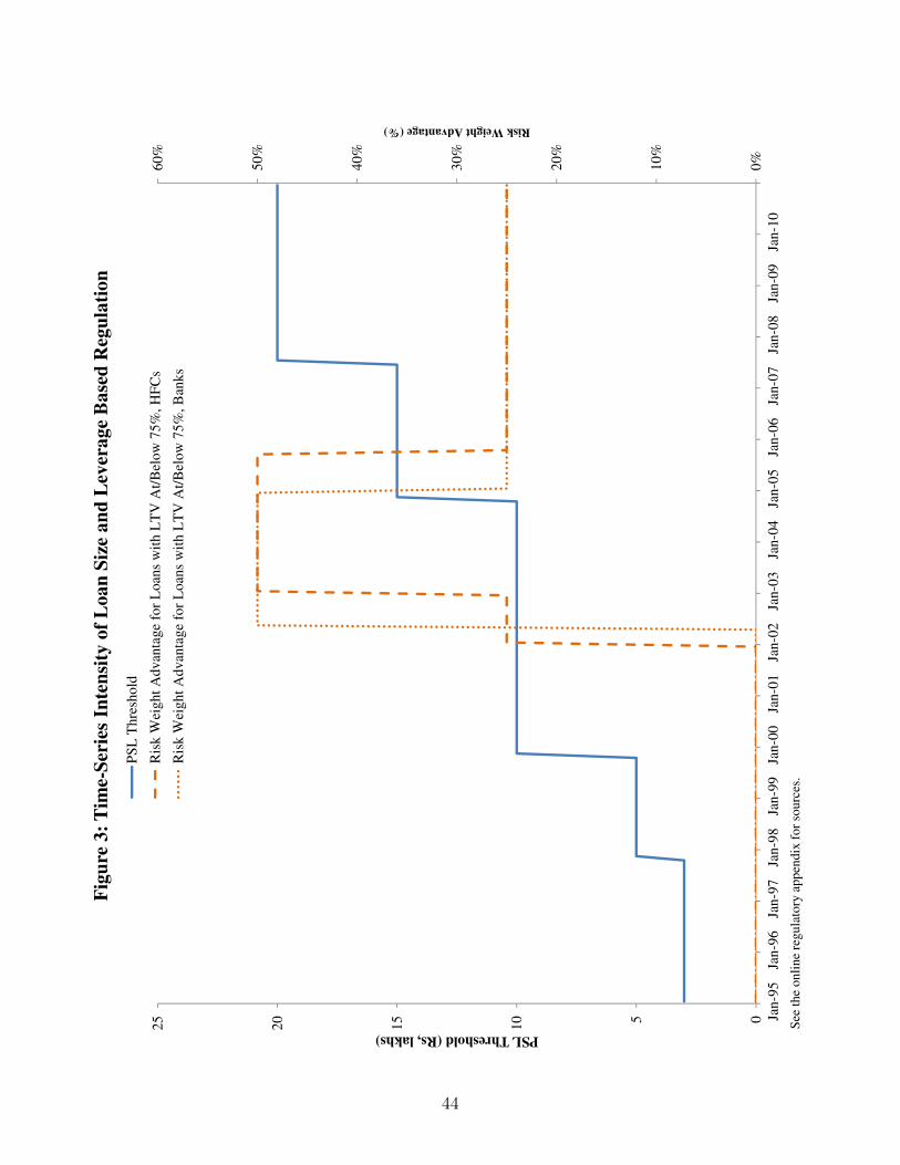
0%

10

%

20

%

30

%

40

%

50

%

60

%

05

10

15

20

25 Ja

n-9

5Ja

n-9

6Ja

n-9

7Ja

n-9

8Ja

n-9

9Ja

n-0

0Ja

n-0

1Ja

n-0

2Ja

n-0

3Ja

n-0

4Ja

n-0

5Ja

n-0

6Ja

n-0

7Ja

n-0

8Ja

n-0

9Ja

n-1

0

Risk Weight Advantage (%)

PSL Threshold (Rs, lakhs)

Fig

ure

3:

Tim

e-S

erie

s In

ten

sity

of

Lo

an

Siz

e a

nd

Lev

era

ge

Ba

sed

Reg

ula

tio

n

PS

L T

hre

sho

ld

Ris

k W

eig

ht

Ad

van

tag

e fo

r L

oan

s w

ith

LT

V A

t/B

elo

w 7

5%

, H

FC

s

Ris

k W

eig

ht

Ad

van

tag

e fo

r L

oan

s w

ith

LT

V A

t/B

elo

w 7

5%

, B

ank

s

See

th

e o

nli

ne

regu

lato

ry a

pp

end

ix f

or

sou

rces

.

44

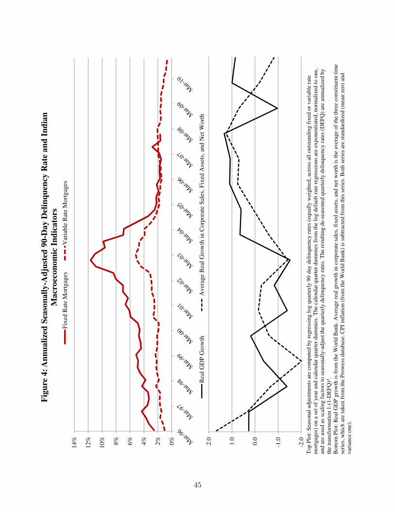
0%

2%

4%

6%

8%

10

%

12

%

14

%

Fig

ure

4:

An

nu

ali

zed

Sea

son

all

y-A

dju

sted

90

-Da

y D

elin

qu

ency

Ra

te a

nd

In

dia

n

Ma

cro

eco

no

mic

In

dic

ato

rs

Fix

ed R

ate

Mo

rtg

ages

Var

iab

le R

ate

Mo

rtg

ages

To

p P

lot:

Sea

son

al a

dju

stm

ents

are

co

mp

ute

d b

y r

egre

ssin

g l

og q

uar

terl

y 9

0 d

ay d

elin

qu

ency

rat

es (

equ

ally

wei

gh

ted

, ac

ross

all

ou

tsta

nd

ing f

ixed

or

var

iab

le r

ate

mo

rtgag

es)

on

a s

et o

f yea

r an

d c

alen

dar

qu

arte

r d

um

mie

s. T

he

cale

nd

ar q

uar

ter

du

mm

ies

fro

m t

he

log d

efau

lt r

ate

regre

ssio

ns

are

exp

on

enti

ated

, n

orm

aliz

ed t

o o

ne,

and

are

use

d a

s sc

alin

g f

acto

rs t

o s

easo

nal

ly-a

dju

st t

he

qu

arte

rly d

elin

qu

ency

rat

es. T

he

resu

ltin

g d

e-se

aso

ned

qu

arte

rly d

elin

qu

ency

rat

es (

DE

FQ

) ar

e an

nu

aliz

ed b

y

the

tran

sfo

rmat

ion 1

-(1

-DE

FQ

)4.

Bo

tto

m P

lot:

Rea

l G

DP

gro

wth

is

fro

m t

he

Wo

rld

Ban

k.

Aver

age

real

gro

wth

in

co

rpo

rate

sal

es, fi

xed

ass

ets,

an

d n

et w

ort

h i

s th

e av

erag

e o

fth

e th

ree

con

stit

uen

t ti

me

seri

es, w

hic

h a

re t

aken

fro

m t

he

Pro

wes

s d

atab

ase.

CP

I in

flat

ion

(fr

om

th

e W

orl

d B

ank)

is s

ub

trac

ted

fro

m t

his

ser

ies.

Bo

th s

erie

s ar

e st

and

ard

ized

(m

ean

zer

o a

nd

var

ian

ce o

ne)

.

-2.0

-1.0

0.0

1.0

2.0

Rea

l G

DP

Gro

wth

Av

erag

e R

eal

Gro

wth

in

Co

rpo

rate

Sal

es,

Fix

ed A

sset

s, a

nd

Net

Wo

rth

45

0.0

%

0.5

%

1.0

%

1.5

%

2.0

%

0.9

70

.98

0.9

91

1.0

11

.02

1.0

3

Delinquency Rate

Lo

an S

ize

Rel

ativ

e to

PS

L T

hre

sho

ld

Fig

ure

5:

Av

era

ge

Del

inq

uen

cy R

ate

s o

f L

oa

ns

Dis

bu

rsed

Nea

r th

e P

SL

Th

resh

old

Dis

bu

rsed

Aft

er R

elax

atio

n o

f P

SL

Co

nst

rain

tD

isb

urs

ed B

efo

re R

elax

atio

n o

f P

SL

Co

nst

rain

t

Eac

h d

ata

po

int

refl

ects

th

e av

erag

e an

nu

al d

elin

qu

ency

rate

fo

r lo

ans

dis

bu

rsed

in

an

in

terv

al o

f 0

.5%

of

the

PS

L t

hre

sho

ld i

n t

he

six

mo

nth

s b

efo

re o

r af

ter

a P

SL

thre

sho

ld r

eset

dat

e. S

tati

stic

s ar

e ag

gre

gat

ed a

cro

ss c

oh

ort

s d

isb

urs

ed a

rou

nd

eac

h o

f th

e fo

ur

PS

L t

hre

sho

ld r

eset

dat

es, u

sin

g a

18

0 d

ay d

efin

itio

n o

f d

elin

qu

eny f

or

19

97

and

19

99

co

ho

rts,

an

d 9

0 d

ay d

elin

qu

ency

fo

r la

ter

coh

ort

s. T

he

ho

rizo

nta

l li

nes

ref

lect

aver

ages

acr

oss

lo

an s

ize

inte

rval

s sp

ann

ing f

rom

0.9

8 t

o 1

.00

, an

d f

rom

1.0

0 t

o

1.0

2 t

imes

th

e P

SL

th

resh

old

.

46

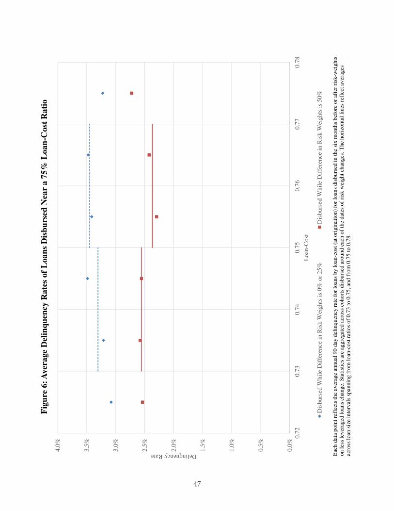
0.0

%

0.5

%

1.0

%

1.5

%

2.0

%

2.5

%

3.0

%

3.5

%

4.0

%

0.7

20

.73

0.7

40

.75

0.7

60

.77

0.7

8

Delinquency Rate

Lo

an-C

ost

Fig

ure

6:

Av

era

ge

Del

inq

uen

cy R

ate

s o

f L

oa

ns

Dis

bu

rsed

Nea

r a

75

% L

oa

n-C

ost

Ra

tio

Dis

bu

rsed

Wh

ile

Dif

fere

nce

in

Ris

k W

eig

hts

is

0%

or

25

%D

isb

urs

ed W

hil

e D

iffe

ren

ce i

n R

isk

Wei

gh

ts i

s 5

0%

Eac

h d

ata

po

int

refl

ects

th

e av

erag

e an

nu

al 9

0 d

ay d

elin

qu

ency

rate

fo

r lo

ans

by l

oan

-co

st (

at o

rigin

atio

n)

for

loan

s d

isb

urs

ed i

n t

he

six

mo

nth

s b

efo

re o

r af

ter

risk

-wei

gh

ts

on

les

s le

ver

aged

lo

ans

chan

ge.

Sta

tist

ics

are

aggre

gat

ed a

cro

ss c

oh

ort

s d

isb

urs

ed a

rou

nd

eac

h o

f th

e d

ates

of

risk

wei

gh

t ch

anges

. T

he

ho

rizo

nta

l li

nes

ref

lect

aver

ages

acro

ss l

oan

siz

e in

terv

als

span

nin

g f

rom

lo

an-c

ost

rat

ios

of

0.7

3 t

o 0

.75

, an

d f

rom

0.7

5 t

o 0

.78

.

47

-1.4

-1.2-1

-0.8

-0.6

-0.4

-0.20

0.2

-12

-11

-10

-9-8

-7-6

-5-4

-3-2

-10

12

34

56

78

91

01

11

2

CID

Fig

ure

7:

Cu

mu

lati

ve

Inst

all

men

t D

efic

it a

rou

nd

Del

inq

uen

cies

Aro

un

d 3

0 D

ay D

elin

qu

enci

es,

18

0 D

ay N

PA

Reg

ime

Aro

un

d 3

0 D

ay D

elin

qu

enci

es,

90

Day

NP

A R

egim

e

-0.4

0

-0.2

0

0.0

0

0.2

0

0.4

0

0.6

0

0.8

0

1.0

0

1.2

0

-12

-11

-10

-9-8

-7-6

-5-4

-3-2

-10

12

34

56

78

91

01

11

2

Difference in CID

Mo

nth

Rel

ati

ve

to D

elin

qu

ency

Mo

nth

Dif

fere

nce

In

CID

Aro

un

d 3

0 D

ay D

elin

qu

enci

es,

Wit

h 9

0%

CI

Pre

dic

ted

cu

mu

lati

ve

inst

allm

ent

def

icit

(C

ID)

is g

iven

by t

he

esti

mat

ed c

oef

fici

ents

on

tim

e to

del

inq

uen

cy (

inte

ract

ed w

ith

a p

ost

-NP

A d

efin

tio

n c

han

ge

du

mm

y)

fro

m a

reg

ress

ion

pre

dic

tin

g c

han

ges

in

th

e cu

mu

lati

ve

inst

allm

ent

def

icit

(val

ue

of

del

inq

uen

t in

stal

lmen

ts i

n t

erm

s o

f ex

pec

ted

mo

nth

ly i

nst

allm

ents

). T

he

po

st-

def

init

ion c

han

ge

du

mm

y a

llo

ws

for

a d

iffe

ren

t p

atte

rn o

f in

stal

lmen

t d

efic

its

to e

mer

ge

aro

un

d d

elin

qu

enci

es f

oll

ow

ing t

he

chan

ge

in r

egu

lato

ry d

efin

itio

n o

f n

on

-

per

form

ing a

sset

s. T

his

mo

del

in

clu

des

tim

e an

d c

oh

ort

fix

ed e

ffec

ts. T

op

Pan

el:

Th

e p

lott

ed s

erie

s ar

e cu

mu

lati

ve

sum

s o

f th

e ch

anges

in

in

stal

lmen

t d

efic

its

esti

mat

ed f

rom

th

e m

od

el w

ith

co

ho

rt a

nd

tim

e fi

xed

eff

ects

rem

oved

. B

ott

om

Pan

el:

Th

e se

ries

sh

ow

n i

s th

e d

iffe

ren

ce i

n t

he

seri

es p

lott

ed i

n t

he

top

pan

el

accu

mu

late

d b

ackw

ard

s an

d f

orw

ard

s in

tim

e fr

om

th

e m

on

th o

f d

elin

qu

ency

. T

he

90

% c

on

fid

ence

in

terv

als

sho

wn

are

co

mp

ute

d b

y b

oo

tstr

app

ing y

ears

of

ob

serv

atio

ns

sep

arat

ely f

rom

bef

ore

an

d a

fter

th

e N

PA

def

init

ion c

han

ge.

48

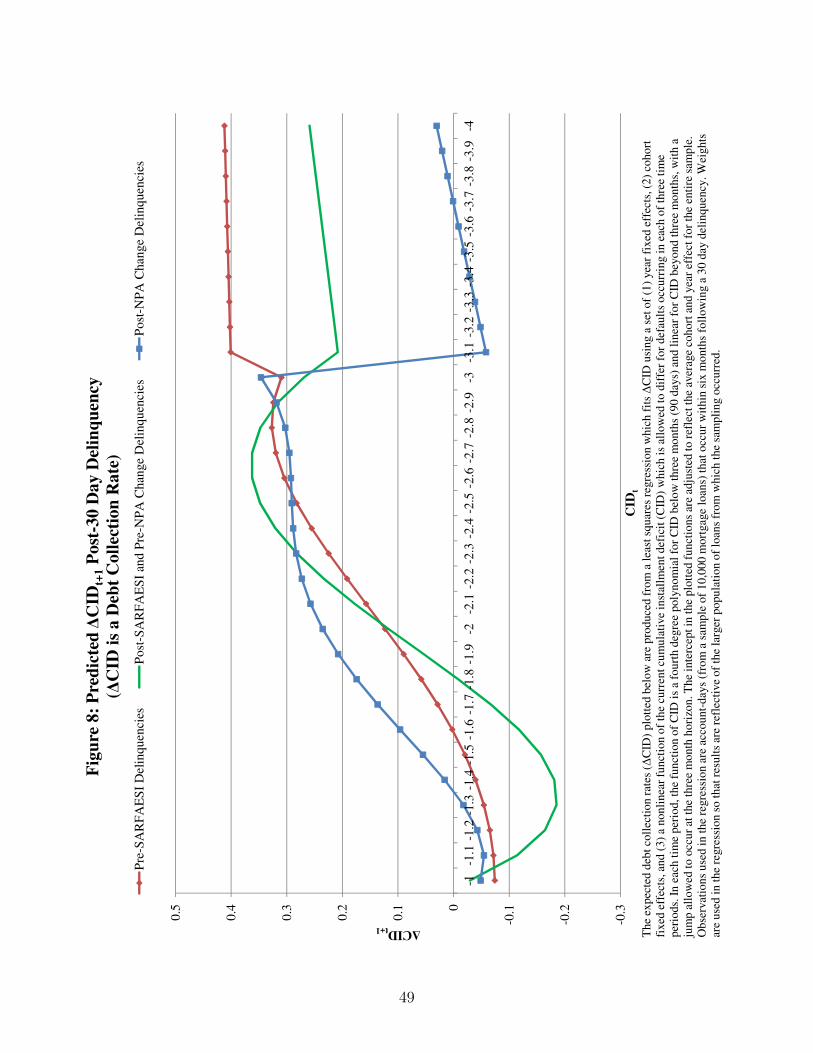
-0.3

-0.2

-0.10

0.1

0.2

0.3

0.4

0.5

-1-1

.1-1

.2-1

.3-1

.4-1

.5-1

.6-1

.7-1

.8-1

.9-2

-2.1

-2.2

-2.3

-2.4

-2.5

-2.6

-2.7

-2.8

-2.9

-3-3

.1-3

.2-3

.3-3

.4-3

.5-3

.6-3

.7-3

.8-3

.9-4

∆CIDt+1

CID

t

Fig

ure

8:

Pre

dic

ted

∆C

IDt+

1P

ost

-30

Da

y D

elin

qu

ency

(∆C

ID i

s a

Deb

t C

oll

ecti

on

Ra

te)

Pre

-SA

RF

AE

SI

Del

inq

uen

cies

Po

st-S

AR

FA

ES

I an

d P

re-N

PA

Ch

ang

e D

elin

qu

enci

esP

ost

-NP

A C

han

ge

Del

inq

uen

cies

Th

e ex

pec

ted

deb

t co

llec

tio

n r

ates

(∆

CID

) p

lott

ed b

elo

w a

re p

rod

uce

d f

rom

a l

east

sq

uar

es r

egre

ssio

n w

hic

h f

its ∆

CID

usi

ng a

set

of

(1)

yea

r fi

xed

eff

ects

, (2

) co

ho

rt

fix

ed e

ffec

ts, an

d (

3)

a n

on

lin

ear

fun

ctio

n o

f th

e cu

rren

t cu

mu

lati

ve

inst

allm

ent

def

icit

(C

ID)

wh

ich

is

allo

wed

to

dif

fer

for

def

ault

s o

ccu

rrin

g i

n e

ach

of

thre

e ti

me

per

iod

s. I

n e

ach

tim

e p

erio

d, th

efu

nct

ion

of

CID

is

a fo

urt

h d

egre

e p

oly

no

mia

l fo

r C

ID b

elo

w t

hre

e m

on

ths

(90

day

s) a

nd

lin

ear

for

CID

bey

on

d t

hre

e m

on

ths,

wit

h a

jum

p a

llo

wed

to

occ

ur

at t

he

thre

e m

on

th h

ori

zon

. T

he

inte

rcep

tin

th

e p

lott

ed f

un

ctio

ns

are

adju

sted

to

ref

lect

th

e av

erag

e co

ho

rt a

nd

yea

r ef

fect

fo

r th

e en

tire

sam

ple

.

Ob

serv

atio

ns

use

d i

n t

he

regre

ssio

n a

re a

cco

un

t-d

ays

(fro

m a

sam

ple

of

10

,00

0 m

ort

gag

e lo

ans)

th

at o

ccu

r w

ith

in s

ixm

on

ths

foll

ow

ing a

30

day

del

inq

uen

cy. W

eigh

ts

are

use

d i

n t

he

regre

ssio

n s

o t

hat

res

ult

s ar

e re

flec

tive

of

the

larg

er p

op

ula

tio

n o

f lo

ans

fro

m w

hic

h t

he

sam

pli

ng o

ccu

rred

.

49

0.1

%

1.0

%

10

.0%

10

0.0

%

-12

-10

-8-6

-4-2

0

Ch

an

ge

in C

ID i

n t

he

Yea

r F

oll

ow

ing

th

e F

irst

30

Da

y D

elin

qu

ency

Fig

ure

9:

Cu

mu

lati

ve

Em

pir

ica

l D

istr

ibu

tio

n o

f C

ha

ng

e in

CID

12

Mo

nth

s P

ost

-30

Da

y

Del

inq

uen

cy

Pre

-SA

RF

AE

SI

Del

inq

uen

cies

(T

hro

ug

h J

un

e 2

00

2)

Po

st-S

AR

FA

ES

I an

d P

re-N

PA

Ch

ang

e D

elin

qu

enci

es

Po

st-N

PA

Ch

ang

e D

elin

qu

enci

es

Ch

anges

in

cu

mu

lati

ve

inst

allm

ent

def

icit

(C

ID)

over

a o

ne

yea

r p

erio

d a

re r

egre

ssed

on

(1

) a

set

of

du

mm

ies

ind

icat

ing i

f a

30

day

del

inq

uen

cy f

irst

occ

urr

ed 1

, 2

,

3..

.12

mo

nth

s ag

o,

(2)

coh

ort

fix

ed e

ffec

ts, an

d (

3)

tim

e fi

xed

eff

ects

. T

hes

e re

gre

ssio

ns

are

run

sep

arat

ely f

or

each

of

the

thre

e ti

me

per

iod

s in

dic

ated

. T

he

cum

ula

tive

dis

trib

uti

on

fu

nct

ion

s p

lot

the

resi

du

al p

lus

fitt

ed v

alu

e o

n t

he

"12

mo

nth

s af

ter

30

day

del

inq

uen

cy"

du

mm

y.

Wei

gh

ts a

re u

sed

in

th

e re

gre

ssio

ns

and

co

nst

ruct

ion

of

the

CD

Fs

so t

hat

res

ult

s ar

e re

flec

tive

of

the

larg

er p

op

ula

tio

n o

f lo

ans

fro

m w

hic

h t

he

sam

ple

was

dra

wn

. F

or

the

rou

gh

ly 1

0%

of

loan

s w

hic

h l

eave

the

bo

oks

wit

hin

a

yea

r o

f th

e 3

0 d

ay d

elin

qu

ency

, th

e C

ID a

t th

e ti

me

of

the

loan

's t

erm

inat

ion

is

use

d i

n t

he

dis

trib

uti

on

.

50

0.1

%

1.0

%

10

.0%

10

0.0

%

-12

-10

-8-6

-4-2

0

Tw

elv

e M

on

th C

ha

ng

e in

CID

Fig

ure

10

: C

um

ula

tiv

e E

mp

iric

al

Dis

trib

uti

on

of

Ch

an

ge

in C

ID f

or

Lo

an

s D

isb

urs

ed

Aro

un

d t

he

NP

A D

efin

itio

n C

ha

ng

e

Lo

ans

Dis

bu

rsed

in

th

e S

ix M

on

ths

Pri

or

to t

he

NP

A C

han

ge

Lo

ans

Dis

bu

rsed

in

th

e S

ix M

on

ths

Fo

llo

win

g t

he

NP

A C

han

ge

Th

e cu

mu

lati

ve

inst

allm

ent

def

icit

s u

sed

are

bas

ed o

n o

bse

rvat

ion

s o

f p

aym

ent

his

tori

es f

or

34

2 m

ort

gag

es d

isb

urs

ed i

n t

he

six

mo

nth

s p

rio

r to

an

d 4

45

mo

rtgag

es

dis

bu

rsed

in

th

e si

x m

on

ths

foll

ow

ing t

he

NP

A d

efin

itio

nch

ange

ado

pti

on

by o

ur

len

der

. T

he

Ko

lgo

rov-S

mir

no

v t

est

stat

isti

c fo

r th

e d

iffe

ren

ce i

n t

he

two

CD

Fs

has

a

p-v

alu

e o

f ab

ou

t 0

.04

.

51