the impact of school district consolidation on housing prices · the impact of school district...

The Impact of School District Consolidation on Housing Prices

609

National Tax JournalVol. LXI, No. 4, Part 1December 2008

Abstract - This paper estimates the capitalization of school district consolidation into housing prices in New York State between 1990 and 2000. We utilize fi rst differencing and 2SLS to account for district heterogeneity and possible endogeneity of the consolidation decision. We fi nd that consolidation boosted house values and rents by about 25 percent in very small school districts and that this effect declines with district enrollment, as expected based on economies of size. Consolidation has no impact on housing prices in districts with more than about 1,700 pupils. The impact of consolidation on housing prices declines with tract house value and rent and is negative in the highest–price tracts.

INTRODUCTION

Ever since Oates (1969), economists have recognized that any change in the property tax or perceived quality of

the local public school system is likely to have an important impact on housing demand and, therefore, on housing prices in the affected communities. This paper applies this insight to school district consolidation.

School district consolidation has been one of the most dramatic changes in education governance and management in the United States in the last century. The number of U.S. school districts declined from 128,000 in 1930 to 14,805 in 1997 (National Center for Education Statistics (NCES) 2006, Table 84). The trend in New York state mirrors the trend in the nation; the number of school district in New York dropped from 9,950 in 1925 to 719 in 1990 (Pugh, 1994).

School district consolidation is no longer as common as it once was, but some states still encourage districts to consoli-date. Districts receive extra aid for “reorganization,” which usually means consolidation, in New York and at least seven other states (NCES 2001).1 Some also encourage consolidation through their building or transportation aid formulas (Haller and Monk, 1988), although several states also discourage consolidation by giving additional aid based on sparsity or small scale (Huang, 2004).

Yue HuWisconsin Center for Education Research,School of Education,University of Wisconsin–Madison,Madison, WI 53706

John YingerCenter for Policy Research, Syracuse University, Syracuse, NY 13244–1020


1 Consolidation, reorganization, and merger are used interchangeably in this paper.

NATIONAL TAX JOURNAL

610

For two reasons, New York State has experienced a resurgence of school district consolidation since the mid 1980s. First, the consolidation incentives in New York’s education aid programs were increased dramatically in 1983. A consolidated school district is eligible for additional formula operating aid over 14 years and additional building aid for both approved renovation and new construction for projects begun within ten years of consolidation. Accord-ing to the 1983 legislation, districts that consolidate received a 20 percent increase in formula operating aid (ten percent in the 1965 legislation) for fi ve years, decreasing two percent each year afterwards, and end-ing after 14 years. In the case of building aid, the matching rate bonus for consoli-dating districts was increased from 25 to 30 percentage points (Spear and Payton, 1992).2

Second, the implementation of the Regents Action Plan in the mid 1980s contributed to the increased interest in reorganization (Spear and Payton, 1992). The Regents Action Plan imposes requirements to expand both the number and type of courses that students must complete to receive a high school diploma in New York. As a result, some districts, especially the very small ones, most likely rural districts, had to broaden their cur-riculums and fi nd classrooms to house the added courses.

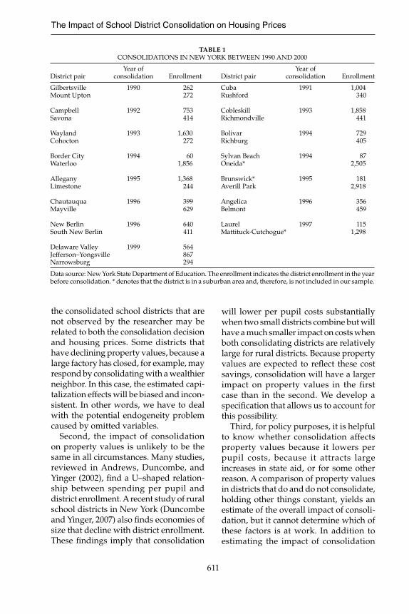
Not surprisingly, consolidation is a particularly appealing option to small rural school districts. In fact, among the 31 school districts that have consolidated since 1990, only three small suburbs are not classifi ed as rural. Table 1 presents some statistics on the consolidations that have taken place since 1990, such as the year of consolidation and the enrollment

before consolidation. The majority of these school districts had an enrollment below 1,000 the year before consolidation. Con-sidering the fact that more than 40 percent of all American schools are in rural areas and 30 percent of all students attend rural schools (NCES, 2006), the focus on rural consolidation in this study may shed light on issues of importance in many states other than New York.

The main source of the consolidation trend in this country appears to be the belief that consolidation leads to lower costs per pupil as a result of economies of size. Several studies, which are reviewed below, have explored the accuracy of this belief. Consolidation has other effects, however, which may be more diffi cult to estimate. Consolidation may lower competition among school districts, for example, or it may raise the transportation costs of students and their parents. As a result, we attack this issue from a differ-ent angle by asking how much parents value district consolidation as refl ected by how much they are willing to pay to live in a school district that has recently consolidated with a neighboring district. Thus, we ask whether the people who buy housing perceive net benefi ts from consolidation due to economies of scale or other sources. Our analysis draws not only on studies of economies of size, but also on studies of the causes of consolidation (Brasington, 1999; Gordon and Knight, 2006).

We begin with a conceptual discus-sion that illustrates the channels through which consolidation could affect housing prices. Building on this discussion, we show that any empirical estimate of the impact of consolidation faces three key challenges. First, some characteristics of

2 The purpose of the incentive aid is to cover immediate costs incurred with consolidation. These costs include a single salary schedule for all states in the reorganized school district, added classrooms to house classes, new uniforms and textbooks for the students and, in some cases, greater transportation costs. According to NYSED (2006), the operating incentive is now up to 40 percent for some districts.


611

the consolidated school districts that are not observed by the researcher may be related to both the consolidation decision and housing prices. Some districts that have declining property values, because a large factory has closed, for example, may respond by consolidating with a wealthier neighbor. In this case, the estimated capi-talization effects will be biased and incon-sistent. In other words, we have to deal with the potential endogeneity problem caused by omitted variables.

Second, the impact of consolidation on property values is unlikely to be the same in all circumstances. Many studies, reviewed in Andrews, Duncombe, and Yinger (2002), fi nd a U–shaped relation-ship between spending per pupil and district enrollment. A recent study of rural school districts in New York (Duncombe and Yinger, 2007) also fi nds economies of size that decline with district enrollment. These fi ndings imply that consolidation

will lower per pupil costs substantially when two small districts combine but will have a much smaller impact on costs when both consolidating districts are relatively large for rural districts. Because property values are expected to refl ect these cost savings, consolidation will have a larger impact on property values in the first case than in the second. We develop a specifi cation that allows us to account for this possibility.

Third, for policy purposes, it is helpful to know whether consolidation affects property values because it lowers per pupil costs, because it attracts large increases in state aid, or for some other reason. A comparison of property values in districts that do and do not consolidate, holding other things constant, yields an estimate of the overall impact of consoli-dation, but it cannot determine which of these factors is at work. In addition to estimating the impact of consolidation

TABLE 1CONSOLIDATIONS IN NEW YORK BETWEEN 1990 AND 2000

District pair

GilbertsvilleMount Upton

CampbellSavona

WaylandCohocton

Border CityWaterloo

AlleganyLimestone

ChautauquaMayville

New BerlinSouth New Berlin

Delaware ValleyJefferson–YongsvilleNarrowsburg

Year of consolidation

1990

1992

1993

1994

1995

1996

1996

1999

Enrollment

262 272

753 414

1,630 272

601,856

1,368 244

399 629

640 411

564 867 294

District pair

CubaRushford

CobleskillRichmondville

BolivarRichburg

Sylvan BeachOneida*

Brunswick*Averill Park

AngelicaBelmont

LaurelMattituck-Cutchogue*

Year of consolidation

1991

1993

1994

1994

1995

1996

1997

Enrollment

1,004 340

1,858 441

729 405

872,505

1812,918

356 459

1151,298

Data source: New York State Department of Education. The enrollment indicates the district enrollment in the year before consolidation. * denotes that the district is in a suburban area and, therefore, is not included in our sample.


612

alone on property values, therefore, we also estimate a model that separates the property–value impacts of enrollment change, school aid change, and other fac-tors associated with consolidation.

Only one previous study has explored the effects of school district consolidation on property values, namely, Brasington (2004). Using housing transaction data from Ohio in 1991, this study fi nds that school district consolidation lead to a 3.5 percentage drop in constant–quality housing values. This pioneering study has extensive data on housing characteristics, but it does not address any of the three problems identified above. Brasington (1999) also contributes to an understand-ing of the potential endogeneity problem discussed above by showing that property values may infl uence the decision to con-solidate, but he does not incorporate this insight into his later study of the impact of consolidation on property values.

The paper is organized as follows. The second section provides a con-ceptual framework. We discuss the potential sources of economies of size associated with school district consolida-tion and develop a formal model of the link between consolidation and property values. The third section describes our data set, and the fourth section describes our estimating strategy. Our results are presented in the fi fth section. These results indicate the extent to which school district consolidation affects property values in New York State. The sixth section presents our conclusions.

CONCEPTUAL FRAMEWORK

The principal reason consolidation is expected to influence property values and rents is that it allows small school

districts to take advantage of economies of size. In this context, the defi nition of “scale” is school district “enrollment” or “size.”3 As we use the term, economies (diseconomies) of size exist if the esti-mated elasticity of education costs per pupil with respect to enrollment, holding student performance constant, is less than (greater than) zero.

Sources of Economies of Size

Although consolidation is often expected to engage economies of size, the literature fi nds sources of both econo-mies and diseconomies of size in educa-tional production. Three main sources of economies of size have been identifi ed.4 The fi rst one is a price privilege associ-ated with larger size; large districts can negotiate bulk purchases of supplies and equipment. The second one is related to specialization. Tholkes (1991) pointed out that large school districts are able to effi ciently utilize specialized labor, such as math and science teachers, and special-ized facilities, such as science and com-puter labs. Finally, administrative costs per pupil may be lower in large schools because central administrative staff and support personnel, such as counselors, can be shared by many students.

Several potential sources of disecono-mies of size also appear in the literature. Tholkes (1991) argued that price disad-vantages also exist as teacher unions are more apt to organize in larger districts, and wages are typically “leveled up” to those of the most generous district. These possibilities may be particularly relevant for rural areas because one of the objectives of consolidation is to provide competitive salaries so that the new district can attract and retain qual-

3 Alternative measures of scale include the quality or scope of educational services. See Duncombe and Yinger (1993).

4 See Andrews et al. (2002) or Duncombe and Yinger (2007) for a detailed discussion.


613

ity teachers. A second potential source of diseconomies of size, which also appears to be particularly relevant in rural areas, is higher transportation costs. Consolidated districts usually pool pupils in similar grades in the same building, which gen-erally results in longer average commute times.5 Another factor that could lead to diseconomies of size is lower student and staff motivation and parental involvement in larger schools. Cotton (1996) and Barker and Gump (1964) argue that in smaller schools students have a greater sense of belonging to the school community and school personnel are more apt to know students by name and to identify and assist students at risk of dropping out. In addition, school administration may be less fl exible in larger schools, and parents of children in larger schools may fi nd it less rewarding to participate in and moni-tor school activities.

As indicated earlier, Duncombe and Yinger (2007) fi nd evidence that the factors leading to economies of size dominate in rural school districts and that economies of size weaken as district size goes up. In addition, they fi nd that consolidation involves substantial adjustment costs. Overall, doubling enrollment through consolidation cuts total annual costs per pupil by 31 percent for two 300–pupil districts but by only 14 percent for two 1,500–pupil districts.

The finding that economies of size decline with size (and may eventually disappear or reverse) has two key impli-cations for our study. First, it implies that all consolidations are not alike, and in particular that some consolidations—those involving very small districts—are likely to have a larger impact on per pupil costs and, hence, on property values than others. It is inappropriate, therefore, to

specify a model in which consolidation has the same absolute or percentage impact on property values and rents in every district. As discussed in more detail below, we address this problem with an interaction between consolidation and pre–consolidation enrollment.

The second implication follows from the fact that consolidation cannot take place, at least not in New York, unless it is approved by the voters in all affected districts. Because economies of size, the main benefi t from consolidation, decline with district size and may eventually disappear, the probability that voters will approve consolidation is likely to be smaller in large than in small districts. Moreover, the benefits and costs of consolidation not associated with enroll-ment are likely to vary from one district to the next and to infl uence the decision to consolidate. Because district size and other factors infl uencing the desirability of consolidation are likely to be correlated with property values, any explanatory variable indicating districts that con-solidate is likely to be endogenous. The second implication, in other words, is that variables infl uencing consolidation also may infl uence property values so that their omission biases the coeffi cient of the consolidation variable in a property value regression.

We take two steps to address the poten-tial endogeneity of our consolidation variable. First, we estimate our models in difference form, which is equivalent, in our case, to including fi xed effects, to eliminate the possible bias from omitted time–invariant variables. Second, we address any remaining endogeneity in the consolidation variable by estimat-ing our model using an instrumental variable technique. Our instrumental

5 In addition, Kenny (1982) suggested signfi cant opportunity costs to both students and parents of longer travel time to school resulted from consolidation. This effect does not show up in school district budgets, but might show up in property values.


614

variables procedure is discussed in detail below.

Formal Model

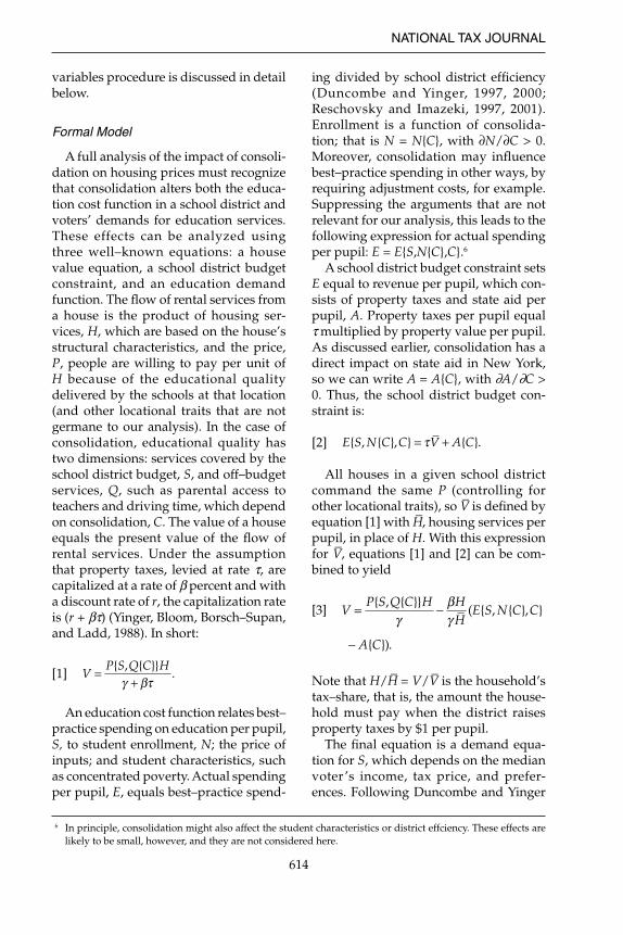
A full analysis of the impact of consoli-dation on housing prices must recognize that consolidation alters both the educa-tion cost function in a school district and voters’ demands for education services. These effects can be analyzed using three well–known equations: a house value equation, a school district budget constraint, and an education demand function. The fl ow of rental services from a house is the product of housing ser-vices, H, which are based on the house’s structural characteristics, and the price, P, people are willing to pay per unit of H because of the educational quality delivered by the schools at that location (and other locational traits that are not germane to our analysis). In the case of consolidation, educational quality has two dimensions: services covered by the school district budget, S, and off–budget services, Q, such as parental access to teachers and driving time, which depend on consolidation, C. The value of a house equals the present value of the fl ow of rental services. Under the assumption that property taxes, levied at rate τ, are capitalized at a rate of β percent and with a discount rate of r, the capitalization rate is (r + βτ) (Yinger, Bloom, Borsch–Supan, and Ladd, 1988). In short:

[1] VP S Q C H=

+{ , { }}

.γ βτ

An education cost function relates best–practice spending on education per pupil, S, to student enrollment, N; the price of inputs; and student characteristics, such as concentrated poverty. Actual spending per pupil, E, equals best–practice spend-

ing divided by school district effi ciency (Duncombe and Yinger, 1997, 2000; Reschovsky and Imazeki, 1997, 2001). Enrollment is a function of consolida-tion; that is N = N{C}, with ∂N/∂C > 0. Moreover, consolidation may infl uence best–practice spending in other ways, by requiring adjustment costs, for example. Suppressing the arguments that are not relevant for our analysis, this leads to the following expression for actual spending per pupil: E = E{S,N{C},C}.6

A school district budget constraint sets E equal to revenue per pupil, which con-sists of property taxes and state aid per pupil, A. Property taxes per pupil equal τ multiplied by property value per pupil. As discussed earlier, consolidation has a direct impact on state aid in New York, so we can write A = A{C}, with ∂A/∂C > 0. Thus, the school district budget con-straint is:

[2] E S N C C V A C{ , { }, } { }.= +τ

All houses in a given school district command the same P (controlling for other locational traits), so V– is defi ned by equation [1] with H–, housing services per pupil, in place of H. With this expression for V–, equations [1] and [2] can be com-bined to yield

[3] VP S Q C H H

HE S N C C

A C

= −

−

{ , { }}( { , { }, }

{ }).

γβγ

Note that H/H– = V/V– is the household’s tax–share, that is, the amount the house-hold must pay when the district raises property taxes by $1 per pupil.

The fi nal equation is a demand equa-tion for S, which depends on the median voter’s income, tax price, and prefer-ences. Following Duncombe and Yinger

6 In principle, consolidation might also affect the student characteristics or district effciency. These effects are likely to be small, however, and they are not considered here.


615

(2000), we fi nd expressions for income augmented by aid and for tax price from the median voter’s budget constraint: YM = Z + (r + τ)VM, where Z is spending on everything except housing and property taxes. By again solving equation [2] for τ and substituting the result into this voter budget constraint, we fi nd that YM + (VM/V–)A{C} = Z + (VM/V–)E{S,N{C},C}. This expression makes it clear that state aid, A, is a component of the median voter’s full income. Moreover, the tax price faced by the median voter, MC, is the derivative of the last term with respect to S, which is a function of C, or MC = MC{C}. Suppress-ing the arguments that are not relevant for our analysis, we can, therefore, write this demand function as follows:

[4] S = S{A{C}, MC{C}}.

Now we can totally differentiate equa-tions [3] and [4] with respect to V, S, and C. This leads to the following expression for the impact of consolidation on house values:7

[5]

The term defi ned by the fi rst two pairs of square brackets on the right side of equation [5] shows the impact of con-solidation on the net value of school services delivered through the district budget. Consolidation–induced increases

in A and decreases in MC (the fi rst pair of brackets) both lead to higher S.8 An increase in S leads in turn to higher V so long as the marginal value of this increase, as refl ected in the rental fl ow, is greater than the marginal cost, weighted by tax share (the second pair of brackets). Voters have no reason to increase S unless this condition holds, so this term is likely to be positive.

The term in the third pair of square brackets begins with the impact of house-holds’ valuation of school services outside the school budget. If consolidation lowers the value of these services, this impact is negative. The next three parts of this term refer to cost savings from economies of scale, adjustment costs, and state aid increases associated with consolidation, respectively. Consolidation increases N and, with economies of scale, lowers the cost per pupil, E. Consolidation also increases A. Hence, the fi rst and last of these expressions are positive. If a district experiences adjustment costs when it con-solidates, the second expression is

negative. Because they operate through a school district budget, these last three expressions are all weighted by a house-hold’s tax share.

This analysis provides valuable per-spective on our study of the housing

dVdC

SA

AC

SMC

MCC

Hr

PS r

HH

MC= ∂∂

∂∂

+ ∂∂

∂∂

⎡⎣⎢

⎤⎦⎥

∂∂

−⎡⎣

β( )⎢⎢

⎤⎦⎥

+ ∂∂

∂∂

− ⎛⎝⎜

⎞⎠⎟

∂∂

∂∂

+ ∂∂

− ∂∂

⎛⎝

H PQ

QC r

HH

EN

NC

EC

ACγ

β⎜⎜

⎞⎠⎟

⎡

⎣⎢

⎤

⎦⎥.

7 To keep the presentation manageable, our conceptual framework does not consider the possibility that con-solidation changes the identity of the median voter. To consider this case, we would have to add a series of terms capturing changes in the responsiveness of the community demand function to income and tax price as a result of a consolidation–induced change in the median voter. Our estimating equation will pick up this effect, but Brasington’s (1999) results, which indicate that districts with signifi cantly different property values are unlikely to merge, suggest that it is likely to be small. We also do not consider the impact of consolida-tion–induced housing price changes on H. Estimates of this price elasticity are quite low. Zabel (2004), for example, obtains a price elasticity of 0.01. Thus, adding this response would add complexity without much insight into consolidation.

8 With a standard multiplicative cost function, the sign of ∂MC/∂C is the same as the sign of ∂E/∂N. The standard multiplicative cost function is E = KSσ f {N{C}}, where K represents all factors other than S and N. In this case, MC = σE/S. Hence, ∂MC/∂C = (σ/S)(∂E/∂N)(∂N/∂C). If consolidation results in economies of size, therefore, ∂MC/∂C < 0.


616

price impacts of consolidation. First, it is clear that consolidation may alter both public service quality and local property tax rates. Voters will not give up $1 of their consolidation–induced property–tax savings and convert it into service quality improvements unless these improvements are worth at least $1 to them. In principle, the service quality improvements could be worth more than $1, so that impact on housing price might depend on the mix of tax cuts and service improvements.

Of course, education quality and the property tax rate may change for reasons other than consolidation. We do not want to control for these changes because that approach would undermine our ability to isolate the impact of consolidation. If we do not control for them, however, we face another potential source of endogeneity: factors that infl uence changes in service quality or the property tax rate may also infl uence the decision to consolidate. This observation reinforces the need to treat consolidation as endogenous.

Our approach to this issue differentiates our study from Brasington (2004), who estimates the impact of consolidation after controlling for service quality and tax rate. As a result, Brasington is not estimating the impact on house values of consolida-tion–induced economies of size or state aid increases, because these impacts will show up in the service–tax package. Instead, he is estimating what people are willing to pay for consolidation–induced factors that fall outside the school budget. This interpretation is consistent with the one given by Brasington. He fi nds a 3.5 percent (or $2,929) decline in constant–quality house value associated with school district consolidation and interprets this as a sign that consolidation restricts the median voter’s control over school out-comes and that the median voter would be willing to pay to avoid this loss of control.

Second, this analysis makes it clear that consolidation can infl uence housing prices through at least four different channels: its

impact on economies of size, its impact on state aid, its impact on adjustment or other costs not associated with enrollment, and its impact on school services delivered outside the district budget. These chan-nels have quite different implications for public policy. The main policy question is whether consolidation can result in costs savings by producing economies of size. An estimate of the impact of consolidation on housing prices does not isolate this impact but instead captures the impact of all these channels put together.

To shed light on the role of these chan-nels, our fi rst step is to estimate our main models with an interaction between con-solidation and pre–consolidation enroll-ment. This approach makes it possible to determine whether the impact of con-solidation is larger for smaller districts, as predicted by the economies–of–size effect. In other words, this approach can test the view that economies of size are at work.

In the second step, we estimate a model to determine whether the housing price impacts of consolidation are linked to changes in state aid, as well as to initial enrollment. The new variable in this model is the change in state aid. This variable is, of course, endogenous because the decision to consolidate results in a large state aid increase. Our strategy for addressing this endogeneity is discussed below.

Our third step is designed to shed some light on the other channels by investigat-ing variation in the impact of consolida-tion across households. All of the terms in equation [5] are multiplied by H, which varies across households. Our strategy is to interact consolidation with 1990 housing price, which is proportional to H, relative to the average housing price in the set of districts that will make up its new district after consolidation. Because we already account for economies of scale and state aid, equation [5] indicates that this interaction term could pick up one of three things: the net benefi ts from


617

consolidation–induced increases in S; the benefi ts, which could be negative, from consolidation–induced changes in Q; or the added taxes to pay for adjustment costs associated with consolidation.

If two consolidating districts have significantly different housing prices, one more possibility must be considered, namely, that consolidation has different impact in different districts because it alters tax shares. Although this possibil-ity was not considered in the derivation of equation [5], it is equivalent to allow-ing the denominator of tax share, H–, to vary with consolidation. Households in a district that has higher property value per pupil than the district or districts with which it merges will experience a decline in H– and, hence, an increase in their tax share.9 This increase in tax share will cause a decline in the amount these households are willing to pay for housing in the district once it consolidates, all else equal. The opposite effect—and, hence, an increase in housing prices—will occur in districts that have a lower property value per pupil than do their new partner(s) in a consolidation. As shown by equation [5], these changes in tax share will lower the net benefi ts from service increases (the last term in the fi rst line) and will raise the negative impact of adjustment costs (the

second–to–last term in the second line). These tax–share effects can only arise in districts with higher pre–consolidation property values than their new partners. This fact makes it possible to separate these effects from others in our estimat-ing equation.

DATA DESCRIPTION

We estimate the impact of consolidation on housing prices using the Geolytics Com-pany’s Neighborhood Change Database (NCD) for New York State in 1990 and 2000, a variation of census data; data from the New York State Education Depart-ment; and school district maps from NCES. The dependent variable and a number of housing characteristics, demographics, and economic characteristics come from NCD data. The NCD data are collected at the census tract level, which is the small-est geographic unit that can be matched across multiple census years. Each census tract usually contains approximately 4,000 people. Our data set includes all census tracts in 228 rural school districts in New York State.10 After dropping 154 observa-tions with missing values, the sample contains about 2,850 census tracts.

Our dependent variables are average house values and rents.11 The average

9 In principle, consolidation also might affect the median voter’s tax–share, which would show up in equation [2]. This effect appears to be very small in New York State (see Duncombe and Yinger, 2007), and we ignore it here.

10 A school district is defi ned as rural if its urban population is less than 30 percent (NCES, 2006). We exclude census tracts in non–rural school districts because, as noted in the text, the consolidation of non–rural school districts is rare. Following the logic of the no–support condition in program evaluation, therefore, we might obtain misleading estimates of the impact of consolidation if non–rural districts were included.

11 Ideally, we would also like to conduct analysis based on median house values and rents. It turns out, however, that the median house values data obtained from the Geolytics Company’s NCD for New York State in 1990 are unreliable. NCD is a panel data set of census tracts based on 2000 census tract boundaries. In 2000 the mean and median house values are reasonably close to each other in New York State. In New York in 2000, for example, the mean of the median house values is $175,133 and the overall mean is $207,785. In 1990, however, the mean of the census tract median house values in New York State is only $106,824, compared with an overall mean of $215,825. This remarkable gap between overall mean and the mean of median in 1990 is probably caused by the procedure used to form consistent data that are based on 2000 census tract boundaries. In particular, in order to construct a panel data based on 2000 census tract boundaries (the census tract boundaries have changed since 1990), the data in 1990 have to be reconfi gured somehow to match the 2000 tract boundaries. The derived median values may have nothing to do with the true median values if the census tract boundaries have changed dramatically across years. These problems do not appear to be as large with rents; in 1990, the median housing rent was 681 and the overall mean rent was 685. For consistency, however, we use the mean rent.


618

house value in each tract is derived from the data for owner–occupied single–fam-ily houses by dividing aggregate house value by the number of housing units. Average housing rents are derived in the same manner based on the sample of renter–occupied housing units. Housing characteristics and demographics include variables such as number of bedrooms, age of the house, percentage population that is black, and percentage household with public assistance income, etc.

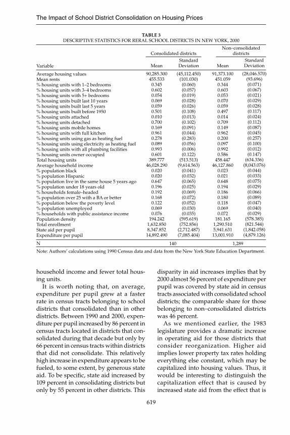
Table 2 and Table 3 present descriptive statistics of our data in 1990 and 2000. Census tracts located in consolidated

school districts are listed separately from those belonging to non–consolidated school districts to facilitate comparisons. The indicator for consolidation equals one if a school district merged with another after 1990 and equals zero otherwise. In our sample, 28 rural school districts containing a total of 140 census tracts consolidated in the 1990s.

In both years, real average housing value is slightly lower in census tracts within a consolidated school district than those in a non–consolidated district.12 Moreover, census tracts in consolidated school districts have relatively lower

TABLE 2DESCRIPTIVE STATISTICS FOR RERAL SCHOOL DISTRICTS IN NEW YORK, 1990

Variable

Average housing valuesMean rents% housing units with 1–2 bedrooms% housing units with 3–4 bedrooms% housing units with 5+ bedrooms% housing units built last 10 years% housing units built last 5 years% housing units built before 1950% housing units attached% housing units detached% housing units mobile homes% housing units with full kitchen% housing units using gas as heating fuel% housing units using electricity as heating fuel% housing units with all plumbing facilities% housing units owner occupiedTotal housing unitsAverage household income% population black% population Hispanic% population live in the same house 5 years ago% population under 18 years old% households female–headed% population over 25 with a BA or better% population below the poverty level% population unemployed% households with public assistance incomePopulation densityTotal enrollmentState aid per pupilExpenditure per pupil

N

Consolidated districtsNon–consolidated

districts

Mean

92,695.550459.7450.3280.6100.0620.0600.0840.4620.0090.7010.1590.9820.2480.1130.9880.607

360.15832,126.970

0.0160.0110.6270.1940.1530.1410.1220.0690.070

194.805868.957

3,990.9378,012.815

Standard Deviation

(47,212.300)(126.539)(0.074)(0.068)(0.024)(0.025)(0.034)(0.122)(0.010)(0.102)(0.084)(0.018)(0.282)(0.054)(0.009)(0.127)

(483.736)(6,085.603)

(0.038)(0.017)(0.069)(0.030)(0.057)(0.063)(0.048)(0.022)(0.030)

(626.387)(776.280)

(1,244.326)(2,473.193)

Mean

98,157.070458.2250.3430.5940.0630.0620.0950.4570.0130.6890.1490.9790.1810.1260.9880.576

422.41432,372.590

0.0190.0160.6060.1930.1520.1500.1180.0740.067

195.4291,257.6013,843.3987,827.740

Standard Deviation

(38,128.490)(115.661)(0.081)(0.072)(0.027)(0.029)(0.061)(0.125)(0.027)(0.118)(0.082)(0.028)(0.253)(0.092)(0.019)(0.161)

(588.665)(5,937.176)

(0.044)(0.029)(0.086)(0.032)(0.063)(0.081)(0.056)(0.032)(0.031)

(697.597)(773.337)

(1,203.478)(2,207.215)

Note: Authors’ calculations using 1990 Census data and data from the New York State Education Department.

140 1,297

12 Both average house values and rents are adjusted using Consumer Price Index to 2000 dollars.


619

household income and fewer total hous-ing units.

It is worth noting that, on average, expenditure per pupil grew at a faster rate in census tracts belonging to school districts that consolidated than in other districts. Between 1990 and 2000, expen-diture per pupil increased by 86 percent in census tracts located in districts that con-solidated during that decade but only by 66 percent in census tracts within districts that did not consolidate. This relatively high increase in expenditure appears to be fueled, to some extent, by generous state aid. To be specifi c, state aid increased by 109 percent in consolidating districts but only by 55 percent in other districts. This

disparity in aid increases implies that by 2000 almost 56 percent of expenditure per pupil was covered by state aid in census tracts associated with consolidated school districts; the comparable share for those belonging to non–consolidated districts was 46 percent.

As we mentioned earlier, the 1983 legislature provides a dramatic increase in operating aid for those districts that consider reorganization. Higher aid implies lower property tax rates holding everything else constant, which may be capitalized into housing values. Thus, it would be interesting to distinguish the capitalization effect that is caused by increased state aid from the effect that is

TABLE 3DESCRIPTIVE STATISTICS FOR RERAL SCHOOL DISTRICTS IN NEW YORK, 2000

Variable

Average housing valuesMean rents% housing units with 1–2 bedrooms% housing units with 3–4 bedrooms% housing units with 5+ bedrooms% housing units built last 10 years% housing units built last 5 years% housing units built before 1950% housing units attached% housing units detached% housing units mobile homes% housing units with full kitchen% housing units using gas as heating fuel% housing units using electricity as heating fuel% housing units with all plumbing facilities% housing units owner occupiedTotal housing unitsAverage household income% population black% population Hispanic% population live in the same house 5 years ago% population under 18 years old% households female–headed% population over 25 with a BA or better% population below the poverty level% population unemployed% households with public assistance incomePopulation densityTotal enrollmentState aid per pupilExpenditure per pupil

N

Consolidated districtsNon–consolidated

districts

Mean

90,285.300455.5330.3450.6020.0540.0690.0590.5010.0100.7000.1690.9610.2780.0890.9930.601

389.77746,028.290

0.0200.0200.6470.1960.1920.1680.1220.0690.076

194.2421,632.8508,347.85214,892.490

Standard Deviation

(45,112.450)(101.030)(0.060)(0.057)(0.019)(0.028)(0.026)(0.108)(0.013)(0.102)(0.091)(0.044)(0.283)(0.056)(0.006)(0.122)

(513.513)(9,614.563)

(0.041)(0.032)(0.065)(0.025)(0.069)(0.072)(0.052)(0.030)(0.035)

(595.619)(752.856)

(2,712.487)(7,085.404)

Mean

91,373.100451.0590.3440.6030.0530.0700.0590.4970.0140.7090.1490.9620.2000.0970.9920.586

458.44746,127.860

0.0230.0210.6480.1940.1860.1800.1180.0690.072

181.1651,290.5105,941.63113,001.910

Standard Deviation

(28,046.570)(93.696)(0.071)(0.067)(0.021)(0.029)(0.028)(0.117)(0.024)(0.112)(0.087)(0.045)(0.257)(0.100)(0.012)(0.147)

(634.336)(8,043.076)

(0.044)(0.033)(0.075)(0.029)(0.066)(0.089)(0.047)(0.040)(0.029)

(578.385)(821.544)

(1,842.058)(4,879.126)

Note: Authors’ calculations using 1990 Census data and data from the New York State Education Department.

140 1,289


620

due to economies of scale. We will explore this decomposition in more detail in the empirical estimation section.

A key data challenge is the determina-tion of the school district location of each census tract. This challenge has three parts. First, we need to obtain consistent measures of census tract boundaries because these boundaries change over time. Second, school district boundaries also change due to consolidation. Third, we have to match each census tract with its corresponding school district for each year.

The Geolytics Company’s Neighbor-hood Change Database (NCD) provides a panel data set of census tracts that is based on 2000 census tract boundar-ies. This data set solves the fi rst part of our data challenge. As far as the school district boundaries are concerned, the NCES provides 1990 and 2000 school district maps. By overlapping the 1990 school district map and the census tract (NCD) boundary map, we are able to match each census tract with its corresponding school district and main-tain the school district boundaries as they were in 1990. This approach ensures that we can match each tract in a pair of con-solidating districts with the characteristics of its separate non–consolidated district before consolidation. Alternatively, we can also overlay the 2000 school district map on the NCD map to match each census tract with a school district based on 2000 school district boundaries. In this way we can link each tract with the characteristics of the consolidated school district to which it belongs after consolida-tion. These tasks are accomplished using Mapinfo.

ESTIMATION STRATEGY

A general cross–sectional model of housing prices (or rents) can be written as

[6] log( ) ,V )itVV it it i itα β μγ it

where log(Vit) is the logarithm of average housing values (rents) in school district iat time t.13 The indicator variable Cit equals one if district i has experienced consoli-dation at time t. The vector Xit includes determinants of housing prices, such as housing characteristics and neighborhood demographic and socioeconomic charac-teristics. μi is time–invariant unobserved school district heterogeneity. εit is the error term. A version of this equation is estimated by Brasington (2004).

The presence of time–invariant hetero-geneity in equation [6] could be a source of bias in estimating β, which measures the percentage change of house values (rents) associated with school district con-solidation. For example, consolidating and non–consolidating districts could have systematically different unobserved char-acteristics that infl uence housing prices. This problem can easily be solved with our data, however, by estimating equation [6] in difference form so that the time–invari-ant unobservable factors cancel out:

[7] Δ log( ) .Δ ΔV )itVV it it itβ γΔΔΔΔβ itΔΔ

As discussed earlier, the impact of con-solidation on property values is unlikely to be the same in all jurisdictions. According to the estimates in Duncombe and Yinger (2007), for example, economies of size fade as school district enrollment increases, so the net benefi ts of consolidation and, hence,

13 Consolidation takes place at the school district level. For two reasons, however, we estimate our models at the census tract level. First, we want to capture as much variation in housing characteristics as possible. Second, we want to determine whether the impact of consolidation depends on household characteristics, as measured by the tract average. To account for potential heteroscedasticity with this design, our standard errors are clustered at the school district level.


621

the impact of consolidation on property values should be greater for smaller dis-tricts. To account for this possibility, we add another term to our specifi cation, namely, an interaction between the change in the consolidation indicator and a district’s 1990 (i.e., pre–consolidation) enrollment. We expect that the sign of this interaction term will be negative; larger districts will have smaller net benefi ts and smaller property value gains than smaller districts.

The trends of property value may also depend on the starting point. For instance, a district with high property values may have a fl atter trajectory of property value increase than a district with low property values.14 We address this issue by adding the baseline property value to equation [7]. The hypothesis is that we should observe a negative relationship between the baseline characteristics and the change of property values.

Accounting for time–invariant unobserv-able factors is a step in the right direction but is unlikely to eliminate all bias in the estimate of β. As discussed earlier, consoli-dation is a choice made by voters and this choice may be infl uenced by factors that also infl uence property values. Brasington (1999) finds, for example, that current property values help to predict future con-solidation, so unobservable district level trends in property values may infl uence which districts consolidate during a given decade. In addition, we pointed out that our regressions purposely do not control for changes in service quality and property tax rates, but such changes might be correlated with both property values and the decision

to consolidate. As a result, estimates from equation [7] are still subject to endogeneity bias due to time–varying unobservable fac-tors infl uencing both property values and the decision to consolidate. Under these circumstances, unbiased estimates require an instrumental variables procedure.

The challenge in implementing such a procedure is, of course, to fi nd appropri-ate instruments. These instruments must help to predict whether consolidation occurs in the 1990s and not be correlated with the change in property values dur-ing that period. We have identifi ed two instruments that appear to meet these conditions. In a later section, we imple-ment a series of tests to address this claim.

The first instrument is number of consolidations that occurred in a census tract’s county in the 1960s. The number of possible consolidations is limited, and this variable indicates the extent to which possible consolidations have already been used up. Thus, we expect that a larger number of consolidations in the 1960s will lead to a smaller chance of a new consoli-dation in the 1990s. We base this variable on the 1960s instead of the 1970s or 1980s both because more consolidations took place in the earlier decade, which gives us more variation to work with, and because the more distant timing minimizes the chance that the instrument is correlated with unobserved factors that infl uence the change in property values in the 1990s.

Our second instrument is the number of school districts that are contiguous to the school district in which a census tract is located.15 This instrument also refers

14 We would like to thank a referee for pointing out this. 15 As a referee points out, the number of neighboring districts in the 90s is likely to be a result of mergers in

the 70s and 80s and, thus, might be endogenous. To address this issue, we also tried using the number of neighboring districts in the 70s as an instrument. (Since we do not observe the actual number of neighbors in the 70s, we constructed this variable based on information regarding the number of mergers in each county in the 70s and 80s and the number of neighboring districts in the 90s. In particular, we add the number of mergers in the 70s and 80s in each county to the number of neighboring districts that we observe in the 90s.) The estimation results are similasr to those using the number of neighboring districts in the 90s. (The results are available upon request.)


622

to opportunities for consolidation, but it captures both within– and across–county variation in the number of neighboring districts. We expect that a larger number of neighbors will increase the probability of consolidation.

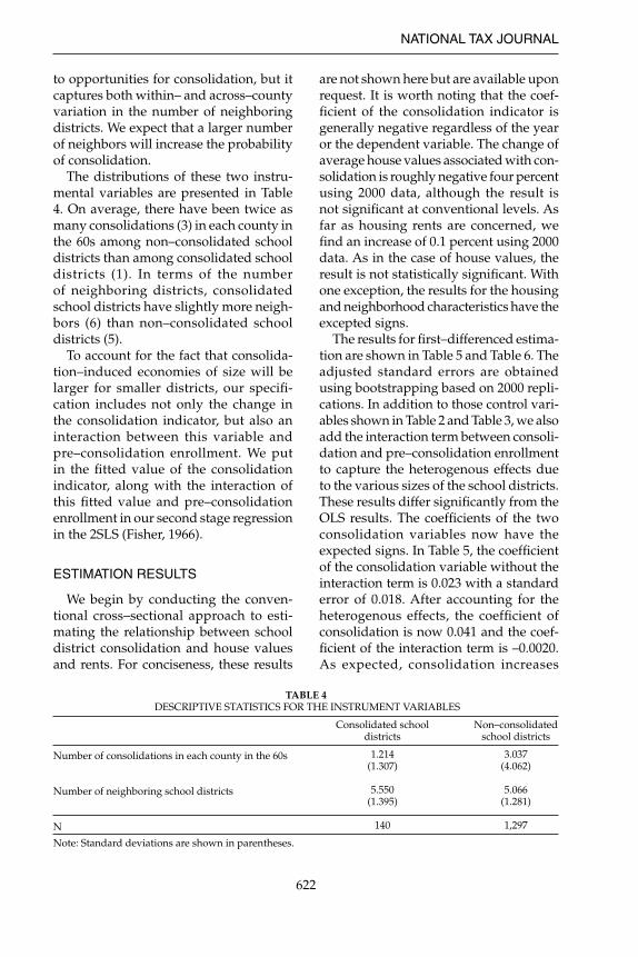
The distributions of these two instru-mental variables are presented in Table 4. On average, there have been twice as many consolidations (3) in each county in the 60s among non–consolidated school districts than among consolidated school districts (1). In terms of the number of neighboring districts, consolidated school districts have slightly more neigh-bors (6) than non–consolidated school districts (5).

To account for the fact that consolida-tion–induced economies of size will be larger for smaller districts, our specifi -cation includes not only the change in the consolidation indicator, but also an interaction between this variable and pre–consolidation enrollment. We put in the fi tted value of the consolidation indicator, along with the interaction of this fi tted value and pre–consolidation enrollment in our second stage regression in the 2SLS (Fisher, 1966).

ESTIMATION RESULTS

We begin by conducting the conven-tional cross–sectional approach to esti-mating the relationship between school district consolidation and house values and rents. For conciseness, these results

are not shown here but are available upon request. It is worth noting that the coef-fi cient of the consolidation indicator is generally negative regardless of the year or the dependent variable. The change of average house values associated with con-solidation is roughly negative four percent using 2000 data, although the result is not signifi cant at conventional levels. As far as housing rents are concerned, we fi nd an increase of 0.1 percent using 2000 data. As in the case of house values, the result is not statistically signifi cant. With one exception, the results for the housing and neighborhood characteristics have the excepted signs.

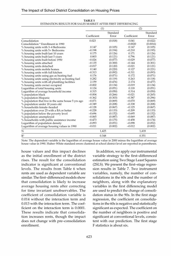
The results for fi rst–differenced estima-tion are shown in Table 5 and Table 6. The adjusted standard errors are obtained using bootstrapping based on 2000 repli-cations. In addition to those control vari-ables shown in Table 2 and Table 3, we also add the interaction term between consoli-dation and pre–consolidation enrollment to capture the heterogenous effects due to the various sizes of the school districts. These results differ signifi cantly from the OLS results. The coeffi cients of the two consolidation variables now have the expected signs. In Table 5, the coeffi cient of the consolidation variable without the interaction term is 0.023 with a standard error of 0.018. After accounting for the heterogenous effects, the coeffi cient of consolidation is now 0.041 and the coef-fi cient of the interaction term is –0.0020. As expected, consolidation increases

TABLE 4 DESCRIPTIVE STATISTICS FOR THE INSTRUMENT VARIABLES

Number of consolidations in each county in the 60s

Number of neighboring school districts

N

Consolidated school districts

1.214(1.307)

5.550(1.395)

140

Non–consolidated school districts

3.037(4.062)

5.066(1.281)

1,297

Note: Standard deviations are shown in parentheses.


623

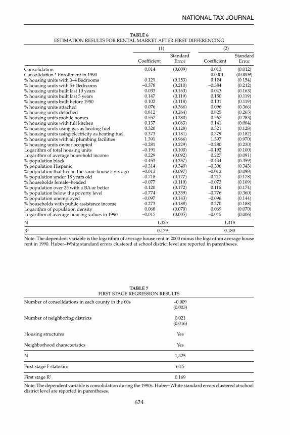
house values and this impact declines as the initial enrollment of the district rises. The result for the consolidation indicator is signifi cant at conventional levels. The results from Table 6 when rents are used as dependent variable are similar. The fi rst–differenced models show that consolidation is likely to increase average housing rents after correcting for time invariant unobservables. The coefficient of consolidation variable is 0.014 without the interaction term and 0.013 with the interaction term. The coef-fi cient on the interaction term is 0.0001. These results indicate that consolida-tion increases rents, though the impact does not change with pre–consolidation enrollment.

In addition, we apply our instrumental variable strategy to the fi rst–differenced estimation using Two Stage Least Squares (2SLS). We present the fi rst–stage regres-sion results in Table 7. Two instrument variables, namely, the number of con-solidations in the 60s and the number of neighbors, along with the explanatory variables in the fi rst differencing model are used to predict the change of consoli-dation status in the 90s. In the fi rst stage regression, the coeffi cient on consolida-tions in the 60s is negative and statistically signifi cant as expected. The coeffi cient on the number of neighbors is positive and signifi cant at conventional levels, consis-tent with our prediction. The fi rst stage F statistics is about six.

TABLE 5ESTIMATION RESULTS FOR SALES MARKET AFTER FIRST DIFFERENCING

ConsolidationConsolidation * Enrollment in 1990% housing units with 3–4 Bedrooms% housing units with 5+ Bedrooms% housing units built last 10 years% housing units built last 5 years% housing units built before 1950% housing units attached% housing units detached% housing units mobile homes% housing units with full kitchen% housing units using gas as heating fuel% housing units using electricity as heating fuel% housing units with all plumbing facilities% housing units owner occupiedLogarithm of total housing unitsLogarithm of average household income% population black% population Hispanic% population that live in the same house 5 yrs ago% population under 18 years old% households female–headed% population over 25 with a BA or better% population below the poverty level% population unemployed% households with public assistance incomeLogarithm of population densityLogarithm of average housing values in 1990

N

R2

Coeffi cient

0.023

0.147–0.198 0.175 0.803–0.026–0.135–0.017 0.140–0.313 0.176 0.282 2.159–0.002 0.124 0.315–0.004–0.362–0.071–0.349–0.128–0.228–0.696–0.065–0.473–0.093–0.011

Standard Error

(0.018)

(0.105)(0.194)(0.126)(0.121)(0.077)(0.300)(0.120)(0.220)(0.092)(0.071)(0.119)(0.476)(0.134)(0.051)(0.050)(0.266)(0.303)(0.069)(0.208)(0.067)(0.133)(0.152)(0.087)(0.175)(0.051)(0.002)

Coeffi cient

0.041 –0.0020 0.147–0.210 0.171 0.796–0.029–0.144–0.021 0.127–0.311 0.172 0.263 2.174–0.019 0.118 0.314–0.021–0.387–0.070–0.338–0.125–0.209–0.695–0.069–0.458–0.098–0.012

Standard Error

(0.022)(0.0016)(0.105)(0.195)(0.126)(0.121)(0.077)(0.301)(0.121)(0.221)(0.093)(0.071)(0.118)(0.477)(0.134)(0.051)(0.050)(0.265)(0.296)(0.069)(0.208)(0.067)(0.133)(0.152)(0.087)(0.174)(0.052)(0.002)

Note: The dependent variable is the logarithm of average house value in 2000 minus the logarithm of average house value in 1990. Huber–White standard errors clustered at school district level are reported in parentheses.

1,425

0.348

1,418

0.351

(1) (2)


624

TABLE 7FIRST STAGE REGRESSION RESULTS

Number of consolidations in each county in the 60s

Number of neighboring districts

Housing structures

Neighborhood characteristics

N

First stage F statistics

First stage R2

–0.009(0.003)

0.021(0.016)

Yes

Yes

1,425

6.15

0.169

Note: The dependent variable is consolidation during the 1990s. Huber–White standard errors clustered at school district level are reported in parentheses.

TABLE 6ESTIMATION RESULTS FOR RENTAL MARKET AFTER FIRST DIFFERENCING

ConsolidationConsolidation * Enrollment in 1990% housing units with 3–4 Bedrooms% housing units with 5+ Bedrooms% housing units built last 10 years% housing units built last 5 years% housing units built before 1950% housing units attached% housing units detached% housing units mobile homes% housing units with full kitchen% housing units using gas as heating fuel% housing units using electricity as heating fuel% housing units with all plumbing facilities% housing units owner occupiedLogarithm of total housing unitsLogarithm of average household income% population black% population Hispanic% population that live in the same house 5 yrs ago% population under 18 years old% households female–headed% population over 25 with a BA or better% population below the poverty level% population unemployed% households with public assistance incomeLogarithm of population densityLogarithm of average housing values in 1990

N

R2

0.014

0.121–0.3780.0330.1470.1020.0760.8120.5570.1370.3200.3731.391

–0.281–0.1910.229

–0.453–0.314–0.013–0.718–0.0770.120

–0.774–0.0970.2730.068

–0.015

Standard Error

(0.009)

(0.153)(0.210)(0.163)(0.119)(0.118)(0.366)(0.264)(0.280)(0.083)(0.128)(0.181)(0.966)(0.229)(0.100)(0.092)(0.357)(0.340)(0.097)(0.177)(0.110)(0.172)(0.359)(0.143)(0.188)(0.070)(0.005)

0.013 0.0001 0.124–0.384 0.043 0.150 0.101 0.096 0.825 0.567 0.141 0.321 0.379 1.397–0.280–0.192 0.227–0.434–0.306–0.012–0.717–0.073 0.116–0.776–0.096 0.270 0.069–0.015

Standard Error

(0.012)(0.0009)(0.154)(0.212)(0.163)(0.119)(0.119)(0.366)(0.265)(0.283)(0.084)(0.128)(0.182)(0.970)(0.230)(0.100)(0.091)(0.359)(0.343)(0.098)(0.178)(0.109)(0.174)(0.360)(0.144)(0.188)(0.070)(0.006)

1,425

0.179

1,418

0.180

(1) (2)

Note: The dependent variable is the logarithm of average house rent in 2000 minus the logarithm average house rent in 1990. Huber–White standard errors clustered at school district level are reported in parentheses.

Coeffi cientCoeffi cient


625

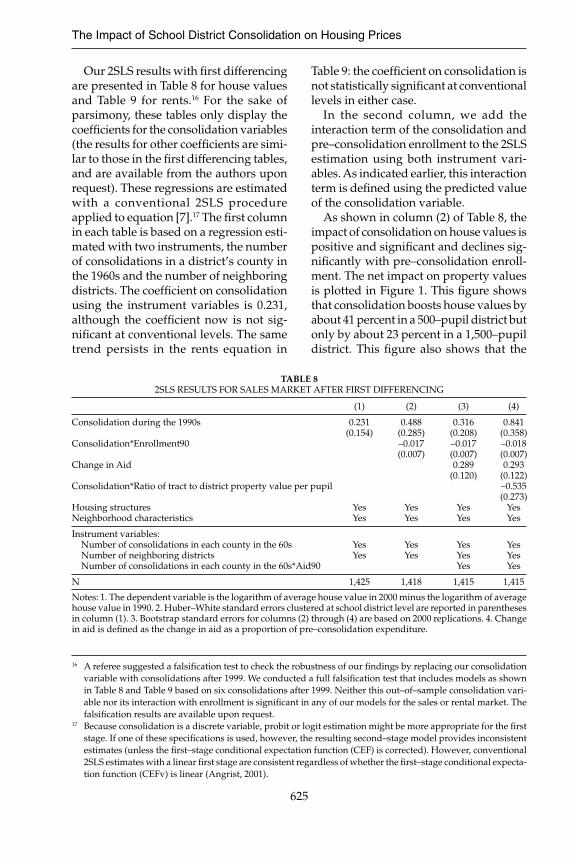
Our 2SLS results with fi rst differencing are presented in Table 8 for house values and Table 9 for rents.16 For the sake of parsimony, these tables only display the coeffi cients for the consolidation variables (the results for other coeffi cients are simi-lar to those in the fi rst differencing tables, and are available from the authors upon request). These regressions are estimated with a conventional 2SLS procedure applied to equation [7].17 The fi rst column in each table is based on a regression esti-mated with two instruments, the number of consolidations in a district’s county in the 1960s and the number of neighboring districts. The coeffi cient on consolidation using the instrument variables is 0.231, although the coeffi cient now is not sig-nifi cant at conventional levels. The same trend persists in the rents equation in

Table 9: the coeffi cient on consolidation is not statistically signifi cant at conventional levels in either case.

In the second column, we add the interaction term of the consolidation and pre–consolidation enrollment to the 2SLS estimation using both instrument vari-ables. As indicated earlier, this interaction term is defi ned using the predicted value of the consolidation variable.

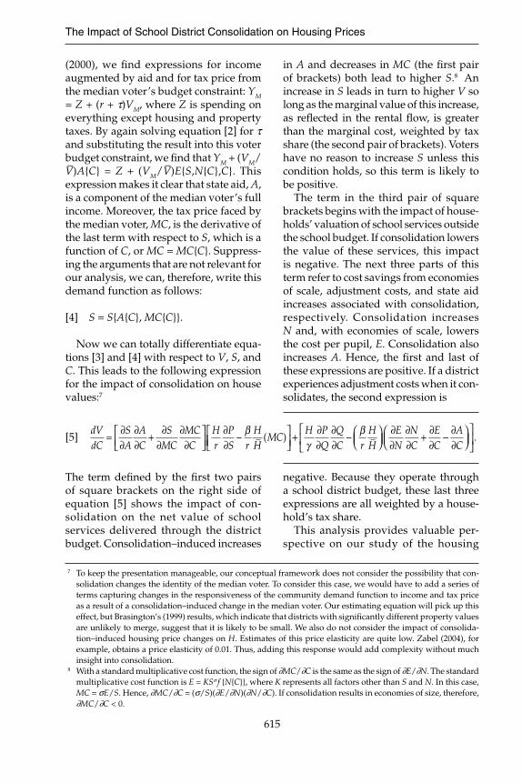
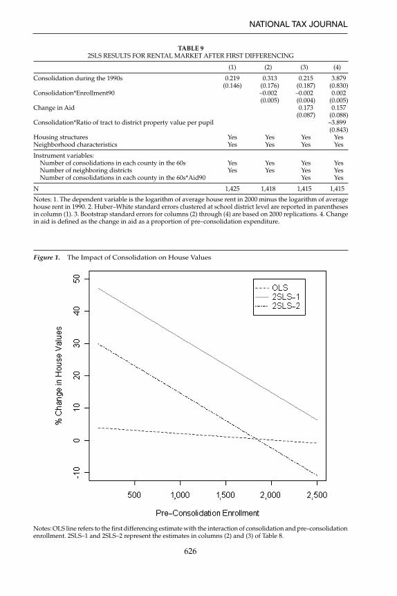
As shown in column (2) of Table 8, the impact of consolidation on house values is positive and signifi cant and declines sig-nifi cantly with pre–consolidation enroll-ment. The net impact on property values is plotted in Figure 1. This fi gure shows that consolidation boosts house values by about 41 percent in a 500–pupil district but only by about 23 percent in a 1,500–pupil district. This fi gure also shows that the

16 A referee suggested a falsifi cation test to check the robustness of our fi ndings by replacing our consolidation variable with consolidations after 1999. We conducted a full falsifi cation test that includes models as shown in Table 8 and Table 9 based on six consolidations after 1999. Neither this out–of–sample consolidation vari-able nor its interaction with enrollment is signifi cant in any of our models for the sales or rental market. The falsifi cation results are available upon request.

17 Because consolidation is a discrete variable, probit or logit estimation might be more appropriate for the fi rst stage. If one of these specifi cations is used, however, the resulting second–stage model provides inconsistent estimates (unless the fi rst–stage conditional expectation function (CEF) is corrected). However, conventional 2SLS estimates with a linear fi rst stage are consistent regardless of whether the fi rst–stage conditional expecta-tion function (CEFv) is linear (Angrist, 2001).

TABLE 8 2SLS RESULTS FOR SALES MARKET AFTER FIRST DIFFERENCING

Consolidation during the 1990s

Consolidation*Enrollment90

Change in Aid

Consolidation*Ratio of tract to district property value per pupil

Housing structuresNeighborhood characteristics

Instrument variables: Number of consolidations in each county in the 60s Number of neighboring districts Number of consolidations in each county in the 60s*Aid90

N

(1)

0.231(0.154)

YesYes

YesYes

1,425

(2)

0.488(0.285)–0.017(0.007)

YesYes

YesYes

1,418

(3)

0.316(0.208)–0.017(0.007)0.289

(0.120)

YesYes

YesYesYes

1,415

(4)

0.841(0.358)–0.018(0.007)0.293

(0.122)–0.535(0.273)

YesYes

YesYesYes

1,415

Notes: 1. The dependent variable is the logarithm of average house value in 2000 minus the logarithm of average house value in 1990. 2. Huber–White standard errors clustered at school district level are reported in parentheses in column (1). 3. Bootstrap standard errors for columns (2) through (4) are based on 2000 replications. 4. Change in aid is defi ned as the change in aid as a proportion of pre–consolidation expenditure.


626

TABLE 9 2SLS RESULTS FOR RENTAL MARKET AFTER FIRST DIFFERENCING

Consolidation during the 1990s

Consolidation*Enrollment90

Change in Aid

Consolidation*Ratio of tract to district property value per pupil

Housing structuresNeighborhood characteristics

Instrument variables: Number of consolidations in each county in the 60s Number of neighboring districts Number of consolidations in each county in the 60s*Aid90

N

(1)

0.219(0.146)

YesYes

YesYes

1,425

(2)

0.313 (0.176)–0.002

(0.005)

Yes Yes

Yes Yes

1,418

(3)

0.215 (0.187)–0.002

(0.004) 0.173

(0.087)

Yes Yes

Yes Yes Yes

1,415

(4)

3.879 (0.830) 0.002

(0.005) 0.157

(0.088)–3.899

(0.843) Yes Yes

Yes Yes Yes

1,415

Notes: 1. The dependent variable is the logarithm of average house rent in 2000 minus the logarithm of average house rent in 1990. 2. Huber–White standard errors clustered at school district level are reported in parentheses in column (1). 3. Bootstrap standard errors for columns (2) through (4) are based on 2000 replications. 4. Change in aid is defi ned as the change in aid as a proportion of pre–consolidation expenditure.

Notes: OLS line refers to the fi rst differencing estimate with the interaction of consolidation and pre–consolidation enrollment. 2SLS–1 and 2SLS–2 represent the estimates in columns (2) and (3) of Table 8.

Figure 1. The Impact of Consolidation on House Values


627

2SLS regression results are quite different from those of the OLS regressions.

Table 9 shows that the consolidation also appears to affect rents. More specifi -cally, the consolidation variable is positive, and signifi cant at conventional levels. The interaction with pre–consolidation enroll-ment is negative, but not signifi cant. These results are plotted in Figure 2. The 2SLS curve has the same general shape as in Figure 1, but the slope is smaller. In short, the impact of consolidation is smaller on rents than on house values. This fi nding suggests that many renters do not believe the property tax savings associated with economies of scale will be passed on to them in the form of lower rents.

Overall, our results demonstrate that in both sales and rental markets, the impact

of consolidation on housing prices cannot be estimated accurately without account-ing for the endogeneity of consolidation. Some of the endogeneity bias is eliminated by differencing (which is equivalent, in our case, to adding fi xed effects because we only have data from two years). This step does not eliminate all of the bias, however, as shown by the large difference between the OLS and 2SLS results for our differenced model.

The third column of Table 8 and Table 9 introduces another variable: the change in state education aid as a proportion of the pre–consolidation expenditure in a school district. This variable is included to determine whether the impact of consolidation on housing prices can be linked to the state aid boost received

Notes: OLS line refers to the fi rst differencing estimate with the interaction of consolidation and pre–consolidation enrollment. 2SLS–1 and 2SLS–2 represent the estimates in columns (2) and (3) of Table 9.

Figure 2. The Impact of Consolidation on Rents


628

by consolidating districts instead of to economies of size or some other factors. As indicated earlier, the change in aid is endogenous. Because we are interested in the impact of aid in consolidating districts, we devise an instrument that is correlated with the expected aid increase in con-solidated districts. As explained earlier, operating aid increases to consolidating districts are governed by a formula based on pre–consolidation aid as a proportion of pre–consolidation expenditure. Thus, our instrument is the pre–consolidation aid expenditure ratio interacted with a consolidation predictor, namely, the share of districts in the county that consolidated in the 1960s.

We fi nd that adding the aid variable lowers the estimated impact of consoli-dation, in both sales and rental markets, which suggests that some share of the property value and rent impact of consoli-dation is, indeed, due to the aid increases that accompany it. In column (3) of Table 8 adding the aid variable lowers the coeffi cient of the consolidation variable from 0.488 to 0.316. In other words, the aid variable accounts for 0.172/0.488 = 35.2 percent of the house–value impact of consolidation in a very small district. The coeffi cient on aid is signifi cant at the one percent level and the consolidation vari-able is not signifi cant. Not surprisingly, adding the aid variable does not alter the slope of the lines in Figure 1; that is, it does not alter the role of economies of size. Instead, adding the aid variable shifts this line downward in a parallel fashion, so that aid accounts for all of the positive impact of consolidation on house values once a district reaches about 1,000 pupils.

Overall, therefore, this attempt to decompose the consolidation effect sug-gests that about one–third of the impact of

consolidation on property values in very small districts is due to the aid increases that accompany consolidation.

The comparable results for the rental market are presented in column (3) of Table 9. Adding the aid variable shifts down the line. The effect due to economies of size remains, but is not signifi cant at conventional levels.

The fi nal column in Tables 8 and 9 adds a variable interacting consolidation with the pre–consolidation housing price in a tract relative to the average housing price in the consolidating districts before consolidation.18 As discussed earlier, this variable should pick up variation across households in the value placed on consoli-dation–induced changes in school quality associated with the district budget (net of tax increases), school quality based on factors outside the school budget, and adjustment costs. It also might refl ect con-solidation–induced changes in tax shares. We fi nd that in both the sales and rental markets, this interaction term has a large, negative coefficient and is highly sig-nifi cant statistically. Because consolidation almost certain yields a positive net benefi t from changes in on–budget school quality, the negative sign on this term appears to rule out the fi rst of these explanations.

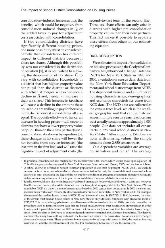
Further information is provided by Fig-ures 3 and 4, which summarize the results from the last column of Tables 8 and 9. As shown in Figure 3, the net impact of con-solidation on house values in small school districts is large and positive in tracts with relatively low house values and moder-ately positive in a tract with house values equal to the district average. In addition, however, the sign of this result reverses in tracts with relatively high house values, even when those tracts are in small school districts where economies of size are large.

18 We also examined two other interaction terms, namely, consolidation interacted with years since consolida-tion (to see if the effects of consolidation phase in) and with income in a district relative to the income in the average district (to see if the impact of consolidation varies with district income). In both cases the estimated coeffcient was close to zero and not close to statistically signifi cant.


629

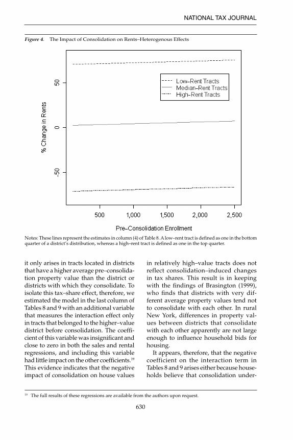
In all types of neighborhoods, the impact of consolidation on house values declines as student enrollment increases and econo-mies of size decline. As shown in Figure 4, a similar pattern holds for rents, although the negative effects in relatively high–rent tracts are even more dramatic and the role of economies of size is much smaller. In fact, Figure 4 indicates that consolidation lowers rents in a tract with the median rent in a district, even when the district is very small. This result contrasts with Figure 2, which indicates a positive impact of consolidation on the average rent in a very small district. These results are not contradictory; rent in a tract with median rent could be, and apparently is, quite different from the district’s average rent.

Based on the conceptual discussion in the second sub–section of the second sec-tion, the negative coeffi cient on the hous-ing–price interaction variable could refl ect one or both of two effects. The fi rst of these effects is the impact on willingness to pay for housing of lost off–budget school ser-vices or adjustment costs associated with consolidation, both of which are propor-tional to housing services (and, hence, to housing price). The second of these effects is the negative impact on willingness to pay for housing of a consolidation–induced tax–share increase. To separate these two effects, we take advantage of the fact that the tax–share effect does not arise in all consolidating tracts with relatively high property values. Instead,

Notes: These lines represent the estimates in column (4) of Table 8. A low–property–value tract is defi ned as one in the bottom quarter of a district’s distribution, whereas a high–property–value tract is defi ned as one in the top quarter.

Figure 3. The Impact of Consolidation on House Values–Heterogenous Effects


630

it only arises in tracts located in districts that have a higher average pre–consolida-tion property value than the district or districts with which they consolidate. To isolate this tax–share effect, therefore, we estimated the model in the last column of Tables 8 and 9 with an additional variable that measures the interaction effect only in tracts that belonged to the higher–value district before consolidation. The coeffi -cient of this variable was insignifi cant and close to zero in both the sales and rental regressions, and including this variable had little impact on the other coeffi cients.19 This evidence indicates that the negative impact of consolidation on house values

in relatively high–value tracts does not reflect consolidation–induced changes in tax shares. This result is in keeping with the fi ndings of Brasington (1999), who fi nds that districts with very dif-ferent average property values tend not to consolidate with each other. In rural New York, differences in property val-ues between districts that consolidate with each other apparently are not large enough to infl uence household bids for housing.

It appears, therefore, that the negative coefficient on the interaction term in Tables 8 and 9 arises either because house-holds believe that consolidation under-

Figure 4. The Impact of Consolidation on Rents–Heterogenous Effects

Notes: These lines represent the estimates in column (4) of Table 8. A low–rent tract is defi ned as one in the bottom quarter of a district’s distribution, whereas a high–rent tract is defi ned as one in the top quarter.

19 The full results of these regressions are available from the authors upon request.


631

mines the quality of off–budget services or that it is associated with large adjustment costs—or both. These results are, there-fore, consistent with the view, expressed in Brasington (2004), that many house-holds are willing to pay to avoid the loss of control associated with consolidation. Indeed, our fi ndings suggest that among households with the “largest” houses, as measured by H, the value placed on the loss of control outweighs the benefi ts from service increases and tax cuts that are made possible by consolidation–induced aid increases and economies of scale. Another possibility is that consolidation leads to increased transportation costs for parents and students and that high–H households value this lost time so highly that it offsets these benefits from con-solidation. The results also are consistent with the fi nding in Duncombe and Yinger (2007) that consolidating rural districts in New York face large adjustment costs that fade out over time. A key issue for future research on consolidation is to provide further evidence concerning the impact of consolidation on off–budget school services, on short–run adjustment costs, and on other factors not considered here.

CONCLUSION

Many states continue to recommend school district consolidation as a way to cut costs, especially in rural areas. This recommendation is supported by research on economies of size in education. Using New York State data, for example, Dun-combe and Yinger (2007) found that con-solidation leads to large cost savings for small rural school districts.

This study complements previous research by examining the impact of school–district consolidation on property values. A focus on property values has the advantage that, at least in principle, it can capture the value voters place on all aspects of consolidation, including but not limited to economies of size. The

value voters place on a loss of control, for example, or on the extra time they and their children spend on getting to school will not be captured by a study that focuses on school district spending.

We show that any study of the impact of consolidation on property values or rents must address three methodological challenges: it must account for the fact that enrollment changes lead to larger cost savings and, hence, larger impacts on property values, in small than in large districts; it must account for the endogene-ity of the consolidation decision; and, at least for policy purposes, it must separate the impacts of state aid changes from economies of size. We address the fi rst challenge by interacting consolidation with pre–consolidation enrollment, and we address the second by estimating our model with both fi rst differencing and instrumental variables.

Our estimates show that a failure to account for either of the fi rst two chal-lenges leads to a striking underestimate of the impact of consolidation on property values. OLS regressions without dif-ferencing fi nds no signifi cant impact of consolidation on housing prices, whereas 2SLS regressions with differencing fi nd large, signifi cant effects that decline with pre–consolidation enrollment. In very small districts, the impact of consolidation on house values approaches 25 percent, but this impact declines to six percent in a district with 1,500 pupils.

Turning to the third challenge, we fi nd some evidence that a signifi cant share of the impact of consolidation on house values is due to the boost in state aid given to districts that consolidate in New York State. The fl ip side of this result is that consolidation still infl uences house values even after controlling for changes in aid, which is a clear sign that factors other than aid are at work. Moreover, the introduction of the aid variable does not alter the coeffi cient that tests for the presence of economies of size. It appears,


632

therefore, that households in very small districts would still perceive net benefi ts from consolidation, due both to economies of size and, perhaps, to other factors that we cannot identify, even if consolidation did not lead to an increase in state aid. Paradoxically, this result indicates that state aid to encourage consolidation is still justifi ed in New York State, at least for very small school districts.

Finally, we explore variation in the impact of consolidation on variation in house values and rents within a school district. We fi nd that consolidation has a large positive impact on house values and rents in tracts with relatively inexpensive housing (as measured before consolida-tion), but a large negative impact in tracts with relatively expensive housing. The most plausible explanation for this result is that consolidation involves adjustment costs and also undermines off–budget school services, such as personal contact between parents and teachers and paren-tal driving time, and that the impact of these factors on housing prices is larger for more expensive housing. Overall, con-solidation appears to be popular with the average household in small rural school districts, but judging by its impact on housing prices, it is not popular among households with relatively valuable hous-ing anywhere in rural New York.

Acknowledgments

We thank Stuart Rosenthal for kindly providing the data. We gratefully acknowledge helpful comments and suggestions from Jan Ondrich, Jeff Kubik, Maria Marta Ferreyra, Kalena Cortes, Christopher Rohlfs, Stacy Chen, William Silky, and two anonymous referees. Yue Hu thanks the Lincoln Institute of Land Policy for fi nancial support. This work was initiated when Yue Hu was a research associate at Center for Policy Research in Syracuse University. The views expressed in the paper should not be attributed to

anyone except the authors. All errors are our own.

REFERENCES

Andrews, Matthew, William D. Duncombe, and John Yinger. “Revisiting Economies of Size in American

Education: Are We Any Closer to a Consen-sus?” Economics of Education Review 21 No. 3 (June, 2002): 245–62.

Angrist, Joshua D. “Estimation of Limited–Dependent Variable

Models with Dummy Endogenous Regres-sors: Sample Strategies for Empirical Prac-tice.” Journal of Business & Economic Statistics 19 No. 1 (January, 2001): 2–16.

Barker, Roger G., and Paul V. Gump. Big School, Small School: High School Size and

Student Behavior. Stanford, CA: Stanford University Press, 1964.

Brasington, David M. “Joint Provision of Public Goods: The Con-

solidation of School Districts.” Journal of Public Economics 73 No. 3 (September, 1999): 373–93.

Brasington, David M. “House Prices and the Structure of Local

Government: An Application of Spatial Statistics.” Journal of Real Estate Finance and Economics 29 No. 2 (September, 2004): 211–31.

Cotton, Kathleen. “Affective and Social Benefi ts of Small–Scale

Schooling.” Eric Digest, Eric Identifier: ED401088 (1996).

Duncombe, William D., and John Yinger. “An Analysis of Returns to Scale in Public

Production, with an Application to Fire Protection.” Journal of Public Economics 52 No. 1 (August, 1993): 49–72.

Duncombe, William D., and John Yinger. “Why Is It So Hard to Help Central City

Schools?” Journal of Policy Analysis and Management 16 No. 1 (Winter, 1997): 85–113.

Duncombe, William D., and John Yinger. “Financing Higher Performance Standards:

The Case of New York State.” Economics of Education Review 19 No. 4 (October, 2000): 363–86.


633

Duncombe, William D., and John Yinger. “Does School District Consolidation Cut

Costs?” Education Finance and Policy 2 No. 4 (Fall, 2007): 341–75.

Fisher, Franklin M. The Identifi cation Problem in Econometrics.

New York: McGraw–Hill, 1966.Gordon, Nora, and Brian Knight. “The Causes of Political Integration: An

Application to School Districts.” NBER Working Paper No. 12047. Cambridge, MA: National Bureau of Economic Research, 2006.

Haller, Emil J., and David H. Monk. “New Reforms, Old Reforms and the

Consolidation of Small Rural Schools.” Educational Administration Quarterly 24 No. 4 (November, 1988): 470–83.

Huang, Yao. “Appendix B: A Guide to State Operating

Aid Programs for Elementary and Second-ary Education.” In Helping Children Left Behind: State Aid and the Pursuit of Educational Equity, edited by John Yinger, 331–52. Cam-bridge, MA: MIT Press, 2004.

Kenny, Lawrence W. “Economies of Scale in Schooling.” Econom-

ics of Education Review 2 No. 1 (February, 1982): 1–24.

National Center for Education Statistics. “Digest of Education Statistics 2005.” Wash-

ington, D.C.: U.S. Department of Education, National Center for Education Statistics, 2006. http://nces.ed.gov/pubsearch/pubsinfo.asp?pubid=2006030. Accessed on September 4, 2008.

National Center for Education Statistics. Public School Finance Programs of the United

States and Canada: 1998–99. Washing-ton, D.C.: U.S. Department of Education, National Center for Education Statistics, 2001.

New York State Education Department. State Aid to Schools: A Primer. Albany, N.Y.:

New York State Education Department, Fis-cal Analysis Unit, 2006. http://www.oms.nysed.gov/faru/Primer/Primer06_07/Primer06-07A.pdf. Accessed on September 9, 2008.

Oates, Wallace E. “The Effects of Property Taxes and Local

Public Spending on Property Values: An Empirical Study of Tax Capitalization and the Tiebout Hypothesis.” Journal of Political Economy 77 No. 6 (November/December, 1969): 957–71.

Pugh, Thomas J. “Rural School Consolidation in New York

State, 1795–1993: A Struggle for Control.” Syracuse University. Ph.D Dissertation, 1994.

Reschovsky, Andrew, and Jennifer Imazeki. “The Development of School Finance

Formulas to Guarantee the Provision of Adequate Education to Low–Income Students.” In Developments in School Finance, edited by William J. Fowler, Jr., 123–47. Washington, D.C.: U.S. Department of Education, 1997.

Reschovsky, Andrew, and Jennifer Imazeki. “Achieving Educational Adequacy Through School Finance Reform.” Journal of Education Finance 26 No. 4 (Spring, 2001): 373–96.

Spear, Suzanne, and Joan Payton. “Analysis of Change in Expenditure Fol-

lowing School District Reorganization.” Albany, N.Y.: New York State Education Department, 1992.

The University of the State of New York. A Guide to the Reorganization of School

Districts in New York State. Albany, NY: New York State Education Depart-ment, School District Organization Unit, undated.

Tholkes, Robert J. “Economies of Scale in Rural School District

Reorganization.” Journal of Education Finance 16 (Spring, 1991): 497–514.

Yinger, John, Howard S. Bloom, Axel Borsch–Supan, and Helen F. Ladd. Property Taxes and House Values: The Theory

and Estimation of Intrajurisdictional Property Tax Capitalization. Boston: Academic Press, 1988.

Zabel, Jeffrey A. “The Demand for Housing Services.” Journal

of Housing Economics 13 No. 1 (March, 2004): 16–35.

the impact of school district consolidation on housing prices · the impact of school district...

Documents