IZA DP No. 3603

The Impact of Social Capital on Crime:Evidence from the Netherlands

I. Semih AkçomakBas ter Weel

DI

SC

US

SI

ON

PA

PE

R S

ER

IE

S

Forschungsinstitutzur Zukunft der ArbeitInstitute for the Studyof Labor

July 2008

The Impact of Social Capital on Crime:

Evidence from the Netherlands

İ. Semih Akçomak Maastricht University, UNU-MERIT

Bas ter Weel

CPB Netherlands Bureau for Economic Policy Analysis, UNU-MERIT, Maastricht University and IZA

Discussion Paper No. 3603 July 2008

IZA

P.O. Box 7240 53072 Bonn

Germany

Phone: +49-228-3894-0 Fax: +49-228-3894-180

E-mail: iza@iza.org

Any opinions expressed here are those of the author(s) and not those of IZA. Research published in this series may include views on policy, but the institute itself takes no institutional policy positions. The Institute for the Study of Labor (IZA) in Bonn is a local and virtual international research center and a place of communication between science, politics and business. IZA is an independent nonprofit organization supported by Deutsche Post World Net. The center is associated with the University of Bonn and offers a stimulating research environment through its international network, workshops and conferences, data service, project support, research visits and doctoral program. IZA engages in (i) original and internationally competitive research in all fields of labor economics, (ii) development of policy concepts, and (iii) dissemination of research results and concepts to the interested public. IZA Discussion Papers often represent preliminary work and are circulated to encourage discussion. Citation of such a paper should account for its provisional character. A revised version may be available directly from the author.

IZA Discussion Paper No. 3603 July 2008

ABSTRACT

The Impact of Social Capital on Crime: Evidence from the Netherlands*

This paper investigates the relation between social capital and crime. The analysis contributes to explaining why crime is so heterogeneous across space. By employing current and historical data for Dutch municipalities and by providing novel indicators to measure social capital, we find a link between social capital and crime. Our results suggest that higher levels of social capital are associated with lower crime rates and that municipalities’ historical states in terms of population heterogeneity, religiosity and education affect current levels of social capital. Social capital indicators explain about 10 percent of the observed variance in crime. It is also shown why some social capital indicators are more useful than others in a robustness analysis. JEL Classification: A13, A14, K42, Z13 Keywords: social capital, crime, the Netherlands Corresponding author: Bas ter Weel CPB Netherlands Bureau for Economic Policy Analysis Department of International Economics PO Box 80510 2508 GM The Hague The Netherlands E-mail: b.ter.weel@cpb.nl

* We benefited from discussions with Lex Borghans, Henri de Groot, Boris Lokshin and Bas Straathof. We acknowledge seminar participants at UNU-MERIT, Maastricht University, CPB Netherlands Bureau for Economic Policy Analysis, the Department of Spatial Economics Vrije Universiteit Amsterdam, ISER University of Essex and the Regional Studies Association meetings in Prague in May 2008. Akçomak acknowledges financial support from the Maastricht Research School of Economics of Technology and Organizations (METEOR).

“The larger and more colorful a city is, the more places there are to hide one’sguilt and sin; the more crowded it is, the more people there are to hide behind.A city’s intellect ought to be measured not by its scholars, libraries, miniaturists,calligraphers and schools, but by the number of crimes insidiously committed onits dark streets...” Orhan Pamuk, My name is Red, p.123.

1 Introduction

One of the most puzzling elements of crime is its heterogeneity across space and not its level

or inter-temporal differences (e.g., Glaeser, Sacerdote, and Scheinkman, 1996; Sampson, Rau-

denbush, and Earls, 1997).1 Even after controlling for economic and social conditions and

population characteristics, there remains a high variance of crime across space. Homicide

rates across comparable and more or less equally developed nations in the European Union

(EU-15) in the 1990s range from on average 12 cases of homicide per million inhabitants in

Sweden, to 28 homicides per million in Finland. Within a sample of Dutch municipalities

(>30,000 inhabitants) crime rates per capita vary between 1.60 in Hof Van Twente (Overijs-

sel) and 14.60 per capita in Amsterdam. Observable factors, such as population density, the

youth unemployment rate, the mean level of education and income inequality can account

for only a small fraction in explaining these differences.2 For example, Utrecht has a crime

rate per capita of 14.3 compared to Leiden with worse observables, which has a crime rate

of only 6.3 per capita.

How can we explain these differences in crime rates across space? We argue that dif-

ferences in social capital can account for a significant part of the observed differences in

crime rates across cities. Criminal behaviour depends not only on the incentives facing the

individual but also on the behaviour of peers or others surrounding the individual. In case

of the same opportunity and expected returns from crime, an individual is less likely to

commit crime if his peers and the community he belongs to punish deviant behaviour. If one

individual decides not to commit crime, it is less likely that others will do so, which creates

an external effect of one person’s behaviour on the others. Informal social control by which

citizens themselves achieve social order increases the level of well-being in a community.1See Freeman (1999) for an overview of the crime literature in economics. Early contributions in economics

by Becker (1968) and Ehrlich (1973) explain the level of crime and the decision to commit crime from aneconomic perspective.

2Glaeser, Sacerdote, and Scheinkman (1996) argue that only about 30 percent of the variance in crimerates across space in the United States can be explained by observable differences in local area characteristics.

1

This in turn raises the level of trust among citizens, altruistic behaviour (e.g., involvement

in charity and voluntary contributions or donations) and participation in activities that serve

the community at a more abstract level (e.g., voting). Although informal social control is

often a response to unusual behaviour, it is not the same as formal regulation and it should

not be equated with formal institutions that are designed to prevent and punish crime, such

as the police and courts. It rather refers to the ability of groups to realise collective goals

and, in our setting, to live in places free of crime.

The empirical part of this research focuses on municipalities (>30,000 inhabitants) in the

Netherlands. We employ a variety of social capital measures. Previous work in economics

and sociology treats social capital as a positive sum.3 Instead of measuring social capital

as a positive value, it might be easier to measure the absence of social capital through tra-

ditional measures of social dysfunction such as, family break down, migration and erosion

in intermediate social structures (Fukuyama, 1996). This approach hinges on the assump-

tion that just as involvement in civic life is associated with higher levels of social capital,

social deviance reflects lower levels of social capital. We benefit from different indicators

such as voluntary contributions to charity, electoral turnout and blood donations as well as

traditional measures of social capital. 4

These indicators seem unrelated and plagued by measurement error if used as individual

indicators of social capital. However, they turn out to be highly correlated and a common

denominator of all these indicators combining several multifaceted dimensions may serve

as a useful and a robust measure of social capital (e.g., Table 2 and Figure 1 below). We

first tackle this problem by treating social capital as a latent construct and form several

social capital indices by using principal component analysis (PCA). Second, we show that

social capital, both represented by individual indicators and by an index, is an important

determinant of crime after controlling for other covariates. We also show that the historical

state of a municipality in terms of population heterogeneity, religiosity and education has an

impact on the formation of current social capital. Our findings reveal that on average a one

standard deviation increase in social capital would reduce crime rates by 0.32 of a standard3Higher social capital is associated with higher economic growth (e.g., Knack and Keefer, 1997); more in-

vestment in human capital (e.g., Coleman, 1988); higher levels of financial development (e.g., Guiso, Sapienza,and Zingales, 2004); more innovation (e.g., Akcomak and ter Weel, 2006) and lower homicide rates (e.g.,Rosenfeld, Messner, and Baumer, 2001).

4Various indicators have been employed to proxy social capital, e.g., generalized trust and membershipto associations, gathered from different surveys like the World Values Survey (WVS) and the EuropeanSocial Survey (ESS). Although these indicators result in consistent and robust findings, their use has receivedcriticism due to inherent measurement error.

2

deviation and that social capital explains about 10 percent of the total variation in crime

rates.

Our approach contributes to the literature in several aspects. First, we treat social capi-

tal as a latent construct and we measure both the presence (e.g., blood donations, voluntary

giving and trust) and absence of social capital (e.g., family breakdown and population het-

erogeneity), which differentiates our study from the existing literature. Simple correlations

between various survey and non-survey indicators of social capital display quite high coeffi-

cients. For instance, the average of the correlation coefficients between survey based trust

and non-survey based social capital indicators − charity, blood and vote − is roughly 0.40.

Second, we try to provide an explanation for how social capital forms. This aspect is largely

ignored in the literature and only took attention recently. In line with Tabellini (2005) and

Akcomak and ter Weel (2006) we argue that the history of a municipality a century ago

does have a significant impact on current levels of social capital. Third, though crime is a

global phenomenon most of the literature is based on the evidence from the United States

(US), the United Kingdom (UK) and Canada.5 The Netherlands has an interesting setting

with homogeneous economic conditions, high concentration of foreigners and a free market

for soft drugs. Finally, our units (municipalities) are much smaller in scale and much more

homogeneous when compared to other studies. So, the results are less likely to be affected

from differences in government policies, laws and regulations. Given the high level of homo-

geneity, the probability of finding a significant correlation between social capital and crime

is low, making us confident of the robustness of our estimates.

This paper proceeds as follows. Section 2 presents the conceptual framework and develops

our arguments. We present information on the data in Section 3. The empirical strategy is

presented in Section 4. Section 5 presents the estimates and a number of robustness checks.

Section 6 concludes.

2 Conceptual framework

Our conceptual framework to study the link between social capital and crime to explain

the heterogeneity of crime through space is based on social capital as a source of control

and community organization. To explain this concept we first explain how we define social5For US see for instance, Glaeser, Sacerdote, and Scheinkman (1996), Freeman (1996),Grogger (1998),

Glaeser and Sacerdote (1999), Gould, Weinberg, and Mustard (2002), Levitt (2004) and Lochner and Moretti(2004). For UK see, Wolpin (1978) and Sampson and Groves (1989) and for Canada see, Macmillan (1995)and McCarthy and Hagan (2001).

3

capital. After that we develop our conceptual framework and the approach taken to explore

the link between social capital and crime.

2.1 Defining social capital

Our definition of social capital is based on four different measures from several different

literatures.

First, social capital is an increasing function of participation in civic life. For instance,

higher voter turnout and more voluntary donations to charity contribute to a community’s

social capital. Voter turnout is hypothesized to capture civic involvement and participation

in community decision making. This indicator is also used by Putnam (1993, 1995), Rosen-

feld, Messner, and Baumer (2001) and Gatti, Tremblay, and Larocque (2003). Voluntary

contributions in money terms are supposed to capture the strength of intermediate social

structures such as charities, clubs and churches and could be employed as another indicator

that measures the presence of social capital. We use a city’s voter turnout rate and its

monetary contribution per household to charity as indicators for social capital.

Second, social capital is higher when people care more for each other or are more altruistic.

To measure this dimension of social capital, Guiso, Sapienza, and Zingales (2004) suggest

to use voluntary blood donations as an indicator for social capital. Although charity and

blood seems to measure similar phenomena there is one particular difference. Experimental

research reports that voluntary contributions may incorporate elements of warm glow (e.g.,

Andreoni, 1995) and reciprocity at the same time. For instance, most charity organizations

send or give small gifts (pens, postcards, etc.) and it has been shown that the contributions

increase with the size of the gift (Falk, 2004). However monetary compensations for donating

blood may even crowd out blood donation as suggested by Titmuss (1970) and recent studies

have shown that this could well be the case (e.g., Mellstrom and Johannesson, 2008). In the

Netherlands there is no monetary compensation of any kind for donating blood, so we suggest

that blood donation captures a pure warm glow effect. We use voluntary blood donations

per capita as a measure of social capital.

Third, security and trust increase the stock of social capital. When there is more con-

formist behaviour, more respect for each other and when norms are institutionalized, the

level of social capital is higher. Trust has been identified as a source of social capital.

Economists defined the concept in a rather lax way, as an optimistic expectation regarding

other agents behaviour (Fafchamps, 2004). Both sociologists and economists have benefited

4

from the survey-based ‘generalized trust’ indicator as a proxy to social capital, which mea-

sures the degree of opportunistic behaviour and as an alternative indicator to social relations

in general (e.g., Putnam, 1995; Knack and Keefer, 1997; Zak and Knack, 2001; Rosenfeld,

Messner, and Baumer, 2001; Messner, Baumer, and Rosenfeld, 2004). The trust indicator is

found to be highly correlated with other measures of social capital such as memberships to

associations, extent of friendship and neighbourhood networks and voting (Putnam, 1995).6

We use a generalized trust index and trust in the police as indicators for social capital.

Finally, informal controls and the extent of informal contacts and acquaintances in-

crease social capital. So far our indicators assume to measure the presence of social capital.

However, the absence of social capital can be measured by using measures of population

heterogeneity and family structure. First, the literature on disadvantaged youth and juve-

nile crime suggests that most criminals come from single-parent households (e.g., Case and

Katz, 1991). Social capital in single-parent households is supposed to be low because of

the fact that they lack a second parent and because they change residence frequently. It

has been shown that single-parenthood has a negative impact on various outcomes, such

as educational attainment, juvenile crime and teenage pregnancy, affecting children’s social

development (e.g., McLanahan and Sandefur, 1994; Parcel and Menaghan, 1994). Second,

population heterogeneity is an important factor that affects social capital and trust as it

breaks closure. We use divorce rates and the percentage of foreigners as indicators of (lack

of) informal control and population heterogeneity.

Empirically, we view social capital as a latent construct that consists of these elements.

In Section 3 the empirical methodology is described in great detail.

2.2 Social control and community organization

Studies of the social environmental characteristics of crime have shown that there exists

a lot of heterogeneity. Disadvantaged neighbourhoods and communities are not equally

plagued by high crime rates. Sampson and Groves (1988) have developed a theory of social

organization in which communities are empowered through their trust in each other to take

action against crime and to join with formal control, such as the police.7 Consistent with this

theory, Sampson, Raudenbush, and Earls (1997) report significantly lower crime levels and

self-reports of victimization in neighbourhoods characterized by social or collective efficacy6Research has shown that the survey-based trust question may measure trustworthiness (Glaeser, Laibson,

Scheinkman, and Soutter, 2000) or well-functioning institutions (Beugelsdijk, 2005) rather than trust itself.7See also Kornhauser (1978), Sampson and Groves (1989) and Bursik and Grasmick (1993).

5

in their study of informal social organization and violent crime in Chicago. Similarly, Bursik

and Grasmick (1993) argue that the effectiveness of law enforcement and public control is

higher in communities with extensive civic engagement.8 Strong attachment and involvement

in community matters also leads to strong social bonds by which conflicts are resolved in a

more peaceful way compared to communities with weak social bonds (e.g., Hirschi, 1969).

Hence, the cost of conflict resolution decreases and more conflicts will be solved.

Communities are stronger when there is lower population turnover and density, because

turnover and density negatively affect the ability to know others and to observe and intervene

in trouble making activities. Glaeser and Sacerdote (1999) explain why there is more crime

in larger cities, and find that larger communities have a more transient and anonymous

character, which reduces social cohesion. This makes it harder to enforce social sanctions,

which reduces the cost of crime and in the end results in more crime. Similarly, Williams and

Sickles (2002) find that by being caught an individual risks to loose the utility generating

social capital (loss of reputation and job, divorce etc.). This means that the more social

capital an individual possesses the higher the expected cost of committing crime, which

reduces the probability to engage in criminal activities. So, given the probability of being

caught and formal control, higher levels of social capital seem to reduce crime.

When people know each other better, they are also more likely to participate in com-

munity organizational life. This is expressed in participation in voluntary organizations and

charity (e.g., Putnam, 1993) and support. The opposite is true for disadvantaged families

and disadvantaged neighbourhoods in which deprivation of any kind feeds further depri-

vation through mechanisms of social interactions and peer effects such as learning effects,

imitation and taking the peers as a role model (e.g., Case and Katz, 1991; Manski, 2000;

Evans, Wallace, and Schwab, 1992). Individuals who belong to these families are more likely

to be unemployed, have low incomes and education and have personal problems. In most

cases divorce rates are higher and families are single-parent families headed by women. They

are also more likely to live in dense areas with a heterogeneous population and more likely

to change residence. Hence, disadvantaged families and persons invest and participate less

in the social community they belong to.8See e.g., Taylor, Gottfredson, and Brower (1984), Sampson and Groves (1989), Land, McCall, and Cohen

(1990), Rosenfeld, Messner, and Baumer (2001), Lederman, Loayza, and Menendez (2002) and Messner,Baumer, and Rosenfeld (2004) for empirical evidence.

6

2.3 Operating the concept

An important issue is that most research on social capital struggles with causality. In this

research, it could be the case that higher crime rates result in out-migration and constrain

positive social interactions. It might also be the case that criminal activity erodes social cap-

ital because it engages individuals in crime networks and keeps them away from educational

and occupational opportunities. We argue that social capital is a positive sum and founded

by historical institutions. Institutions promoting the formation of social capital in the past

are positively correlated with current levels of social capital. Finally, higher levels of social

capital now, result in lower crime rates.

We apply an instrumental variable strategy in which we instrument a city’s current social

capital with its past level education, population heterogeneity and religiosity. Recent studies

have shown the validity of such an approach (Tabellini, 2005; Akcomak and ter Weel, 2006).

We argue that population heterogeneity, the contribution of religiosity to human and social

capital investments, and education in the past contribute to the formation of a city’s social

capital, hence shape current social capital.

If social capital is an asset paving the way to community governance (Bowles and Gintis,

2002) or to achieve goals that could be not be achieved or could be achieved only at an higher

cost (Coleman, 1988), then any factor that would lead to disorganization and dis-attachment

in the community would eventually reduce social capital. Population heterogeneity is such a

factor that may trigger dis-attachment as higher levels of heterogeneity would break closure,

reduce acquaintance among residents and may result in lower trust among members of the

community (e.g., Rose and Clear, 1998; Rosenfeld, Messner, and Baumer, 2001). The effects

of racial and/or ethnic heterogeneity on socio-economic outcomes are well documented in

the literature. It is shown that heterogeneity has an effect on corruption (Mauro, 1995), rent

seeking and low educational attainment (Easterly and Levine, 1997), and lower provision

of public goods (Goldin and Katz, 1999). However, our argument in this paper is that

ethnic and religious heterogeneity may result in circumstances where formal and/or informal

institutions are not binding. Therefore, our argument is more in line with the literature

that links heterogeneity to social capital in the wider sense. For instance, both Easterly

and Levine (1997) and Alesina, Baqir, and Easterly (1999) argue that ethnic fragmentation

may increase polarization in a community and create difficulty in the provision of public

goods such as public education, libraries, and sewer systems. In a similar vein Alesina and

La Ferrara (2000) argue that racial composition affects the degree in participation in social

7

activities. Zak and Knack (2001) and Rupasingha, Goetz, and Freshwater (2002) also show

that higher levels of ethnic diversity may result in less trusting societies.

We argue that Protestant belief may have a dual effect on the formation of social capital,

which is beyond simply saying that being more religious is associated with higher social

capital. First, Beyerlein and Hipp (2005) differentiate between bonding and bridging social

capital and argue that groups characterized by bonding social capital are not effective in

creating an environment of informal social control to deal with the threat of crime, whereas

groups with extensive bridging social capital are more effective in creating such foundations.9

The results show that crime rates are lower in societies with higher levels of bridging social

capital. Given this finding that mainline Protestants are more likely to be involved in

community wide volunteering, which in turn refers to higher levels of social capital, we argue

that communities where more Protestants reside are characterized by a certain environment

and ‘ethic’ to paraphrase Max Weber, in which social capital may nurture. This view stresses

the institutional aspect of Protestantism. A second link is the human capital aspect (Becker

and Woessmann, 2007). The argument here is that Protestant instructions to read the Bible

in ones own language and the support for universal schooling boosted the literacy levels early

on and hence created human capital as a side effect. Previous research by Coleman (1988)

and Goldin and Katz (1999) helps to explain differences in human capital by relating it to

historical differences in social capital. 10

The interaction between human and social capital is well documented in the literature

(e.g., Coleman, 1988; Goldin and Katz, 1999). Here we base our argument on the fact that

human capital affects social capital with a lag. For instance, Goldin and Katz (1999) show

that high school movement in the 1930s in various states in the U.S affects current levels of

social capital. Recent analyses by Tabellini (2005) and Akcomak and ter Weel (2006) support

this finding. They show that for different samples of European regions literacy rates in 1880s

do have an impact on current levels of social capital and on a set of cultural indicators. The

idea here is that education builds human and social capital at the same time. As shown9Bonding social capital are links mainly or exclusively among members of the same group, whereas bridg-

ing social capital links members of different groups among communities. Bonding social capital increasescommunity social capital within groups, but may also reduce overall social capital by restricting links amonggroups. Beyerlein and Hipp (2005) use the percentage of mainline Protestant and Catholics as a proxy forbridging social capital as they involve in community wide volunteering, and the percentage of EvangelicalProtestants as a proxy for bonding social capital because Evangelical Protestants are more likely to involvein voluntary activities within their group but not in a wider community.

10A possible third mechanism may be the ‘guilt’ mechanism. As suggested by Fafchamps (1996) andPlatteau (1994), contractual obligations could be enforced via several mechanisms such as loss of reputationand guilt. Starting from Max Weber numerous studies emphasized how religion might play a role in individualor firm decision making.

8

by Gradstein and Justman (2000, 2002) education affects social capital because education is

an important socializing instrument as it builds common norms and facilitates interaction

between community members who might be different along cultural, religious or ethnic lines.

3 Data and Descriptives

The data span 142 municipalities with more than 30,000 inhabitants in the Netherlands.

We employ the 2002 geographical definition of Dutch municipalities with each municipality

matched to a NUTS regional definition.11 Most of the socio-economic variables come from

Statistics Netherlands (CBS). We restrict our analysis to municipalities with populations

of more than 30,000. For smaller municipalities and for earlier years some variables are

unavailable. Table 1 presents summary statistics for all variables we use in the empirical

analysis. We discuss the most salient details of the most important variables below, and

other variable definitions, sources and details in Appendix 1.

3.1 Social capital

We benefit from several indicators to proxy social capital. Information on voluntary giving,

charity, is obtained from the national fundraising agency (Centraal Bureau Fondsenwerving,

CBF). The original data is available in euro terms and defined as voluntary contributions per

household averaged over the term 2000-2005.12 For the electoral turnout we use the voter

turnout for the elections of the Lower House (Tweede Kamer) in 2003. Following Guiso,

Sapienza, and Zingales (2004) we collected data on blood donations. The data set is for

2005 and comprises information on the number of donations. We define blood as the blood

donations per 100 inhabitants. Higher values of charity, vote and blood are associated with

higher levels of social capital.

To support our data and for robustness purposes we have also gathered data from ESS −

a database designed to measure persistence and change in people’s social and demographic

characteristics, attitudes and values. These survey-based indicators are widely used in the11The 2002 geographical definition of Dutch municipalities is available at Statistics Netherlands (CBS),

http://www.cbs.nl. The NUTS definition is available at eurostat http://ec.europa.eu/eurostat. The Nether-lands are divided into 4 NUTS 1, 12 NUTS 2 and 40 NUTS 3 regions. See Appendix 4 for details.

12We also calculated voluntary givings per inhabitant for each year and then averaged the data over timeto see whether there is any significant difference between the two measures. As expected there is no effecton the results. This calculation introduces some bias because the municipality definitions change every yearfrom 2000 to 2005 and for this reason we use correspondence tables to match municipalities and in cases thatwe have missing population or household information we interpolate the data. Due to these shortcomings weuse the original version of the indicator as available from the source.

9

social capital literature. To increase the sample size we merged the first and the second

round of ESS conducted in 2002 and 2004. The merged data include information on more

than 4,000 individuals. The data is adjusted by population weights to reduce the possibility

of complications that might arise due to over-sampling. We construct an equal weight trust

indicator from the answers to the following three questions and label it trust, (i) ppltrust is

formed from the answers to the following statement: “Most people can be trusted or you can’t

be too careful”, (ii) most people try to take advantage of you, or try to be fair (fair), (iii)

most of the time people are helpful or mostly looking out for themselves (help). For all three

indicators higher values represent higher levels of social capital. To capture the confidence

in institutions we use “trust in police” (formed from the question “How much you personally

trust the police”) from the same source. Unfortunately all these five indicators are only

available for 40 NUTS 3 regions and it is not possible to collect similar information at the

municipality level. However, we include these measures in our analysis by creating variables

that have the same value for municipalities in the same NUTS 3 regional definition.13

We also measure the absence of social capital using traditional measures of heterogeneity

and family structure. We first collected information on the percentage of foreigners in each

municipality as a proxy to population heterogeneity.14 Related to this measure we formed

movers to represent mobility in a municipality. We define movers as the sum of the absolute

value of immigration and emigration divided by the population. To capture erosion in family

induced social capital divorce rates are used as an indicator.15

The correlations among all these indicators are displayed in Table 2 and depicted in

Figure 1. The simple correlations suggest that measures of social capital are strongly cor-

related. Correlations between the individual indicators, charity, blood, vote, trust, foreign

and divorce, are in a range between 0.01 to -0.74 with an average of 0.36.16 As shown in

Appendices 2 to 5 these observations are not restricted to a specific group of municipalities

and hold for different subsamples.17

13For instance, Heerlen (917), Sittard (1883), Maastricht (935), Landgraaf (882) and Kerkrade (928) areall in Zuid-Limburg, hence all five municipalities share the same value for the above indicators from the ESSdatabase.

14To support this measure we also collected data on immigration, emigration and detailed data on foreignersdifferentiating between males and females and between first and second generation immigrants. Introducingsuch differences does not yield different results.

15We also experimented with using the percentage of single parent families/households, which yields similarresults.

16The average calculated by taking the absolute value of each correlation. For NUTS 3 regions the corre-lations range from 0.19 to -0.86, with an average of 0.46.

17We have replicated the analysis for municipalities with more than 40,000 and 50,000 inhabitants respec-tively, for 40 NUTS 3 regions and for 22 largest agglomeration in the Netherlands.

10

To get an idea of how regions and municipalities are distributed along these social capital

indicators we ran a k-means cluster analysis to see whether the data differentiates between

regions with high and low social capital. If the analysis is restricted to two groups there is a

clear distinction between the north and east of the Netherlands, which are rich in terms of

social capital and the south and the west, which are relatively poor in terms of social capital.

If the cluster groups are increased to 4 this distinction still prevails although it is not that

clear anymore. Municipalities in the northern part of the Netherlands tend to have values

that are above the mean for charity, blood, vote and trust and values below mean for foreign

and divorce. In the southern part this pattern is the other way around. In the west and

the east we have mixed groups. This simple preliminary analysis gives another hint that the

social capital indicators tend to move together supporting simple correlations.

Our fundamental premise in this paper is that these variables capture different dimensions

of social capital and even though they may not be very good proxies for social capital

individually, a common denominator of them may stand as a good indicator of social capital.

The final goal is to treat social capital as a latent construct and to form social capital indices

by using principal component analysis (PCA). First, we performed PCA including charity,

blood, vote, trust, foreign and divorce and saved the first principal component as SC1 which

explains about 55 percent of the total variation. This is an overall index merging both

presence and absence of social capital in one measure. Then we formed another index in a

similar way, SC2, only capturing the presence of social capital hence including the first four

indicators above. Due to reasons we have mentioned above about the availability of trust at

the municipality level, we formed a final index, SC3, including only charity, blood and vote

for robustness reasons. The first component explains more than 60 percent of the variation in

these three variables. Further details on the social capital indicators, the principal component

loadings and the explained variance for all included indicators are presented in Appendix

1.2.

3.2 Crime

Information about crime is constructed from the 2002 crime monitor of the Algemeen Dag-

blad. The data yield information on 27 different types of crime.

We form an overall indicator per 100 inhabitants covering all recorded crimes and label

it crime. In the literature there is a tendency to use data for crime that have minimal

reporting inconsistencies such as, motor vehicle theft, robbery and burglary. This is indeed

11

important because the crime numbers include a category for bicycle theft, but especially in

the Netherlands bicycle theft is so common that many people do not even report if they

are victim of bicycle theft. In a similar vein, crime numbers on handling soft drugs could

also be biased since there is a relative free market for soft drugs in the Netherlands. On

the other hand, citizens are more likely to report if their car is stolen. Therefore, as well as

analyzing overall crime rates we have specified nine categories of crime according to the 2006

European Sourcebook of Crime and Criminal Justice. These are homicide, serious assaults,

rape, robbery, theft, motor vehicle theft, burglary, domestic burglary and drug related crimes.

Appendix 1.3 defines each of these categories and presents descriptive statistics for a number

of subsamples. The most important categories of reported crime for our preferred sample

of cities with more than 30,000 inhabitants are robberies and drug related crime. Least

important are burglary and rape.

A more detailed investigation of the crime data produces two main insights. First, most

recorded crime falls into one or two subcategories. For example, overall theft is roughly 55

percent of all recorded crime and roughly 11 percent consists of assaults; whereas serious

crime such as rape and homicide is only 1 percent of overall crime rate. Second, in the

Netherlands most criminal activities take place in larger agglomerations. For instance, among

all recorded homicides 51 percent occurred in the 22 largest cities and about 85 percent were

observed in municipalities with more than 30,000 inhabitants. In extreme cases like robbery

and drug related crime 3 out of 4 attempts are observed in the 22 largest Dutch cities. This

pattern more or less prevails for all categories and even for overall crime rates as 53 percent

of all recorded crime is observed in the 22 largest agglomerations and 83 percent occurs

in municipalities with more than 30,000 inhabitants Table A1.3.2 provides the distribution

of criminal activities for different subsamples. It seems appropriate to argue that criminal

activity in the Netherlands is an urban phenomenon, which supports our choice of sample.

The selection of 142 municipalities represents only about 35 percent of all the municipalities

in the Netherlands but covers over 90 percent of overall crime.

3.3 Instrumental variables

In line with Tabellini (2005) and Akcomak and ter Weel (2006) we suggest that historical

factors do have an impact on the formation of social capital and rely on three indicators as

an instrument for social capital all of which are observed at the municipality level in 1859:

(i) population heterogeneity, (ii) percentage of protestants, (iii) number of schools. All three

12

variables are taken from the population archive (Volkstellingen), which provides historical

data on household, population, occupation etc. starting from 1795 onwards. We selected

1859 because this is the earliest date for which data at the municipality level are available.

More information about the population archive and the three instruments can be found in

Appendix 1.4. Table A1.4 lists the data for the 142 municipalities with more than 30,000

inhabitants.

The percentage of foreigners in 1859 is used as an instrument for current social capital

as it is a proxy for trust in 1859. Municipalities that were well endowed in terms of social

capital 150 years ago may still be rich in social capital, which emphasizes the importance

of initial presence. In this case, past social capital directly affects current social capital but

has no direct impact on current crime levels. We define foreign1859 as the percentage of

foreigners living in a municipality in 1859. We define protestant1859 as the percentage of

inhabitants belonging to any of the Protestant denominations in 1859. We also collected

data on the number of schools in 1859 in each municipality as a direct proxy for human

capital investment different from the effect of Protestantism on human capital formation as

discussed in Section 2. Although it may not be a perfect indicator for human capital in

1859 we believe that it is still a credible instrument to current social capital. #school1859

is defined as number of schools per 1,000 inhabitants.

4 Empirical Strategy

Our empirical strategy hinges on the assertion that social capital is an important determinant

of crime and that social capital is hard to measure and thus should be best treated as a latent

construct. Social capital is different from other forms of capital in the sense that it is not

directly observable. Therefore, our first strategy is to measure social capital as a single

index composed of different indicators that could act as an individual proxy for different

dimensions of social capital. To do so, we use a principal component analysis (PCA) that

estimates

Yi = βisocial capital + εi, (1)

where i corresponds to different indicators of social capital, Y is the latent construct com-

posed of a number of social capital indicators. Estimating this equation yields a number of

principal component factors and a number of principal component loadings, βi, which could

be viewed as weights. Since the indicators are highly correlated with each other we only

13

use the first principal component as a measure of social capital and label it SCx, where

x ranges from 1 to 3 and denotes the inclusiveness of the index. As discussed above we

construct three indices where SC1 is the most inclusive consisting of six indicators and SC3

is the least inclusive consisting of three indicators. Table A1.2 lists the principal component

loadings and the explained variance for each index and for each sample. The first principal

component explains 50 to 65 percent of the variation induced by the indicators.18

Having constructed the indices of social capital we start estimating the following base

model with OLS using usual explanatory variables of crime:

crime = β0 + β1density + β2education + β3unemp

+ β4young + β5SC + ε, (2)

where subscript m for municipalities has been suppressed for notational convenience, and the

error term complies with the usual assumptions. Crime represents crime rates depending on

the type or group of criminal activity. Density refers to population density. To normalize

the data we took the natural log of population density. We expect higher crime rates in

densely populated areas. Education is the percentage of people with medium and high levels

of education. As criminal activity is concentrated within relatively younger age groups,

we have included the percentage of people between 15-24 years old. Unemp represents the

unemployed under age 30. We expect education to be negatively correlated with crime

and the percentage of population 15-24 years old and youth unemployment to be positively

associated with crime. SC represents not only the three indices but also the six individual

indicators to construct the indices.

The next step is to replicate the analysis above for an extended model:

crime = β0 + β1density + β2education + β3unemp

+ β4young + β5SC + β6X + υ, (3)

where X consists of a set of control variables which are; (i) income inequality, (i) controls

for the percentage of area devoted to shopping and recreation activities, and (iii) number

of coffeeshops per 10,000 inhabitants. We expect these variables to be positively correlated

with crime rates.18Recently, a similar strategy was used by Fryer, Heaton, Levitt, and Murphy (2005) to measure the impact

of crack cocaine on crime in U.S. cities.

14

Endogeneity and the possibility of reverse causality could bias the estimates of the above

models when using OLS. Putnam (2000) has argued that low social capital may result in

higher crime, which in turn may result in even lower levels of social capital. For example,

a third unobserved variable could affect both crime and social capital. Certain policies

implemented by the local government could reduce crime but at the same time have an

impact on social capital. Or, it could be the case that crime reporting rates are correlated

with social capital levels, so inhabitants living in high social capital areas may be more likely

to report crime (e.g., Soares, 2004). To deal with such problems we use a 2SLS strategy in

which we instrument social capital with the historical proxies discussed and constructed in

Section 3. We use the percentage of foreigners, protestants and the number of schools in

1859 as instruments for social capital. This yields the following model for estimation:

crime = β0 + β1density + β2education + β3unemp

+ β4young + β5SC + β6X + ν,

SC = δ0 + δ1foreign1859 + δ2protestant1859

+ δ3#school1859 + δ4Z + η, (4)

where foreign1859 stands for the percentage of foreigners and protestant1859 denotes the

percentage of Protestants living in a municipality in 1859. #school1859 is the number of

schools per 100 inhabitants in 1859. The matrix Z includes all other exogenous variables. We

expect foreign1859 to be negatively, and protestant1859 and #school1859 to be positively

correlated with social capital. Since almost all our variables have different measurement

levels we standardized all the variables so that the mean and variance equals 0 and 1,

respectively. Therefore the estimated coefficients are also standardized coefficients measuring

how the dependent variable responds when an independent variable changes by one standard

deviation.

5 Results

5.1 OLS Estimates

We start by estimating the base model (equation 2) using OLS. Table 3 presents the esti-

mates. The dependent variable is defined as the overall crime rates. The mean of this crime

15

measure has been standardized to zero. We observe from the base model that individual

indicators of social capital have significant impact on overall crime rates. Charity, blood,

vote, trust and trustplc are negatively associated with crime, whereas foreign, divorce and

movers are positively correlated with crime rates. With the exception of trust all coefficients

are significant at the 5 percent level.19 Our findings are in line with the previous research

that reports negative effects for trust, civicness and electoral turnout (e.g., Sampson and

Groves, 1989; Rosenfeld, Messner, and Baumer, 2001; Lederman, Loayza, and Menendez,

2002; Messner, Baumer, and Rosenfeld, 2004) and research that finds a positive link between

crime and population heterogeneity (e.g., Jobes, 1999) and single parenthood (e.g., Samp-

son, Morenoff, and Earls, 1999) and crime. Moreover, all three social capital indices have

significant negative effects on crime as can be observed from the last three columns in Table

3. These indices imply that a one standard deviation increase in the social capital index

reduces crime by between 0.29 and 0.35 of a standard deviation. This effect is economically

meaningful, since it means that a one standard deviation increase in social capital would

reduce crime rates by about 2 percent on average.

Our findings on ordinary determinants of crime also support prior evidence. Popula-

tion density generally has a positive and significant effect on crime suggesting that densely

populated areas are more likely to be vulnerable to crime than relatively rural areas (e.g.,

Wolpin, 1978; Macmillan, 1995). This is because heterogeneity and residential instability

reduce the effectiveness of community sanctions. In addition, urban areas attract criminal

activity as there are more opportunities for such activities in cities where they can act rather

anonymously (e.g., Glaeser and Sacerdote, 1999). We find a negative coefficient for edu-

cation suggesting that the higher the level of education the lower the crime rate, which is

also consistent with the literature (Lochner and Moretti, 2004; Wolpin, 1978). This is first

because higher education is associated with better labor-market outcomes hence increasing

the opportunity cost of crime and possibly because school attendance keeps young people

away from the street conditional on the fact that young people commit more crimes (Lochner

and Moretti, 2004). However, only in a few specifications the coefficient is statistically sig-

nificant. The results also show that crime rates are increasing with the percentage of young

people, which is consistent with earlier work (Wolpin, 1978; Freeman, 1996; Grogger, 1998).

The only contradicting result of our estimates is the negative coefficient for the youth unem-19As we have mentioned before trust scores are available at the NUTS 3 level and are merged to data at

the municipality level. This adjustment likely partly explains why the coefficient is statistically insignificant.Similar analysis at the NUTS 3 level (with n = 40) returns a significant coefficient for trust.

16

ployment rate, although the coefficient is statistically insignificant. Oster and Agell (2007)

and Gould, Weinberg, and Mustard (2002) show for a panel of Swedish municipalities and

American cities that a fall in unemployment led to a drastic decrease in drug possession, auto

theft and burglary. However, these results also reveal that changes in youth unemployment

have no particular effect on crime.

After the inclusion of a number of additional control variables the results are qualitatively

similar as the estimates in Table 4 show. All social capital indicators have a statistically

significant impact on crime rates. In the extended model, income inequality has no significant

effect on crime and the sign alternates depending on the specification. Previous research

on the effect of income inequality on crime also shows contradicting results (e.g., Soares,

2004). However, recent research shows that changes in the distribution of income inequality

rather than income inequality itself affect property crime (Bourguignon, Nunez, and Sanchez,

2003; Chiu and Madden, 1998). Another point is that the cross-section analysis we employ

throughout the paper may not be such a suitable approach to assess the importance of

inequality and unemployment on crime rates. Unfortunately, in our setting it is not possible

to pursue panel analysis. This is because we do not have the adequate data to do so and

more importantly because social capital is a stock that does not change from year to year,

whereas inequality and unemployment figures do.

As expected the percentage of recreational and shopping area has a positive and signif-

icant effect on crime (e.g., Jobes, 1999). This is because there are more opportunities for

criminals in such areas and the returns are higher (e.g., Glaeser and Sacerdote, 1999). We

also found quite a strong effect for the percentage of coffeeshops in a municipality on crime

rates. This could be due to several reasons. First, the probability of committing crime may

increase under the influence of soft drugs. Second, coffeeshops attract disadvantaged per-

sons, gang activity and drug dealers which sets up an environment that supports criminal

activity. Finally, to buy drugs, addicted people often have to commit crime. Inclusion of the

four control variables increases the explanatory power by one third suggesting that about 65

percent of the variation in crime is explained by the extended model. The added-variable

plots are presented in Figure 2, which reveal the strong conditional correlations except for

trust.

Table 5 is a summary table presenting the coefficients of all social capital indicators we

consider for different subsamples. It is apparent that all six (charity, blood, vote, foreign,

divorce and movers) non-survey social capital indicators have a significant effect on crime.

17

The survey indicators, trust, ppltrust, help, fair and trustplc, do not return a significant

coefficient all the time. Another potentially interesting result is the impact of emigration

as well as immigration on crime rates. Immigration has a negative effect because it reduces

closure in a community (e.g., Jobes, 1999). Considering the fact that social capital originates

from social interactions within a network, any factor breaking links between actors is harmful

for social capital. In this respect emigration may also increase crime rates. It could also be

the case that individuals who are less integrated in a society are more likely to commit crime,

which is why both immigration and emigration are positively associated with crime rates.

Our indicator movers (capturing both effects) reflects residential instability in a community

and it is positively related to crime suggesting that the higher instability the higher crime

rates, which is consistent wih earlier work (e.g., Rose and Clear, 1998). The social capital

indices are always significant at the one percent level regardless of the specification and the

sample considered.

5.2 2SLS Estimates

The OLS estimates above could be biased because of causality problems. We next explore

a 2SLS strategy instrumenting social capital with the percentage of foreigners, percentage

of Protestants and the number of schools in 1859. Table 6 presents the 2SLS estimates.

Columns (1), (3) and (5) present the first stages of the 2SLS estimations for the three social

capital indices, respectively. The instruments in the first stage have the expected effect on

social capital. The quality of the instruments is important as they should be correlated with

social capital but not with the error term in a way that the instruments should be on the

‘knife’s edge’. If the correlations of the instruments and social capital are not strong enough

in the first stage we run into weak instrument problems. On the other hand, if they are

too strong we cannot safely assume that they are not correlated with the error term. The

joint F-tests in the first stage show that our instruments are valid as they pass the F-test

threshold of 10 suggested by Staiger and Stock (1997). Moreover the over-identification tests

show that the effect of the instruments on crime are operationalized only through their effect

on social capital, not by any other mechanism.

The second stage results reveal that the coefficients of the social capital indices are

somewhat larger than their OLS counterparts and significant at the 1 percent level. These

estimates imply that a one standard deviation increase in social capital reduces crime by

between 0.30 and 0.34 of a standard deviation. This effect is economically meaningful and

18

not far from the estimates from the OLS exercise above (Table 4). The estimates suggest

that the causality runs from social capital to crime and the historical state of a community

shape current social capital.

Complementary to the OLS results above we present summary information on how in-

dividual indicators of social capital behave in 2SLS specification. Table 7 is comparable

to Table 5 and for each subsample and model the first column shows the 2SLS coefficient

derived from the estimation of equation (4) (for the base and the extended model). The

second column shows the associated joint significance test of the instruments in the first

stage. In all specifications the estimations return a significant coefficient in the second stage.

However, the F-tests illustrate an interesting pattern. As can be seen from Table 7, F-tests

for foreign, divorce, vote and charity are larger than (or within the proximity of) 10. Given

this result, we can assert that these indicators cannot only be labeled as good indicators of

social capital, since they are also the ones that display consistent and quite robust estimates

in their relationship with crime. Blood donations do not perform as good as the ones above.

The estimates presented in Tables 4-7 use different measures of social capital and our

social capital indices, which come from treating the concept as a latent construct. In the

theoretical literature on social control, support and networks have been put forward or could

be applied as measures of social capital in relation to crime. In our empirical analysis we

have constructed measures that are by and large consistent with these theoretical concepts.

All measures of social capital turn out to have a significant relationship with crime.

The methodology we employ in this paper allows us to discuss which indicators of social

capital perform best. This is potentially interesting for future research as we can identify

social capital indicators and also their relation to crime. Throughout the paper we have sum-

marized the results for 14 potential social capital indicators and three indices constructed

from these indicators. Indicators related to social support, solidarity and civicness perform

quite well as indicators of social capital. However, electoral turnout and donations to charity

stand out from the rest. Although their relation to crime is mostly significant, blood dona-

tions and trust are found to be rather inferior when compared to charity and vote. This

can be seen from Table A1.2 in Appendix 1. When constructing the indices, the principal

component analysis yields more or less the same weight for charity and vote, but blood and

trust receive only about one third of the weight attached to charity and vote. This discrep-

ancy becomes visible and significant as the sample moves from NUTS3 regions to smaller

municipalities. Our results also show that indicators of social control (divorce rates) and pop-

19

ulation heterogeneity (percentage of foreigners, immigration, emigration and movers) can be

labeled as good social capital indicators. When the principal component loadings of the most

inclusive index (SC1) is inspected carefully one can easily see that charity, vote, foreign

and divorce receive similar weights in magnitude. In almost all specifications charity, vote

and most of the measures of social control and heterogeneity are important determinants of

crime. Blood donations and trust indicators from the ESS database are found to be not as

important as the others.

5.3 Robustness

5.3.1 Subsamples

We perform several robustness checks to validate our results. First, we replicate the analysis

using different subsamples. The detailed results of these exercises are presented in Appendix

2 for 95 municipalities with more than 40,000 inhabitants, Appendix 3 for 63 municipalities

over 50,000 inhabitants, Appendix 4 for 40 NUTS 3 regions and finally Appendix 5 for the

22 largest agglomerations in the Netherlands. This exercise reveals that there are no crucial

differences affecting the results discussed above and that our findings do not seem to be

bound to a specific subsample.

5.3.2 Different Types of Crime

Besides analysis on the overall crime rates we also estimate the extended model (equation

3) for 9 different crime categories. The rationale behind this is the argument that overall

crime rates are biased due to under reporting of certain crime types. Therefore, we have

to show that our results also hold for crime that is supposed to have minimum reporting

inconsistencies such as auto theft, robbery, serious assaults and homicide. Table 9 presents

the expected sign and the significance levels of the impact of different social capital indicators

on crime subcategories and Figure 3 depicts the added-variable plots. The results highlight

several interesting points. With the exception of the social capital indices, the individual

social capital indicators seem to have a weak effect on homicide only. Four indicators yield

significant coefficients. The only subcategory of crime that is found to be affected by all

social capital indicators is serious assaults. The difference in the effect of social capital on

property and violent crimes is also not that important. The only exception to this is that

trust and divorce seem to have more effect on violent crimes when compared to property

crimes. Another interesting result is that charity, vote and foreign have a significant impact

20

on almost all of the crime categories besides their effect on overall crime rates. The other

indicators are sometimes loosely related to crime rates. This point could also be taken as a

point for caution for researchers who employ a single (or few) social capital indicator, as the

results would highly depend on the selection of that particular indicator.

5.3.3 Social Capital Indicators

One of our main arguments in this paper is that the indicators seemingly unrelated are in

fact correlated with each other and represent different dimensions of social capital. Previous

research argues that blood donations and electoral turnout can safely be considered to be

exogenous (e.g., Guiso, Sapienza, and Zingales, 2004). By the same token, one could argue

that divorce rates are exogenous too. However, it could be the case that because of higher

crime, municipalities become more transient and heterogeneous as opportunities attract out-

siders or it could be the case that because of high crime residents are afraid to leave their

homes which affects their civic participation and reduces interpersonal trust (e.g., Liska and

Warner, 1991). As a further robustness check we show what happens if one employs indica-

tors of social capital as instruments for each other. Figure 4 summarizes the results. The

upper and the lower panel represent the 2SLS coefficients and the t-ratios respectively. To

make our point clear we can explain the methodology as following. We instrument each

social capital indicator by the remaining five social capital indicators and estimate 2SLS

models. For instance, for the first box-plot in the upper panel, we use all possible combina-

tions of blood, vote, trust, foreign and divorce − individually, and in groups of 2, 3, 4 and

5 − as instruments to charity and replicate the 2SLS estimation over and over again until

we consume all possible combinations. This produces a set of 2SLS coefficients and t-ratios

for charity and the distribution of these coefficients and t-ratios are depicted as the first

box-plot in the upper and lower panel respectively. This is done for all six indicators and

for each case there are 31 observations (i.e., 31 2SLS coefficients and t-ratios for each social

capital indicator). The (*) indicates the coefficients and the t-ratios of the social capital

indicators from the OLS estimation of equation 3 (see Table 4). The three vertical lines in

the lower panel indicate the significance levels at the 1, 5 and 10 percent level.

From Figure 4, the following observations stand out. First, as can be seen from the lower

panel, all the 2SLS coefficients are significant at least at the 5 percent level. This supports our

argument that all these indicators are related to each other and could be used as instruments

for each other. Including them in the same regression would render serious multicollinearity

21

problems. It was specifically for this reason that we formed social capital indices. Second,

the 2SLS coefficients and t-ratios are somewhat higher than their OLS counterparts. Third,

the 2SLS coefficient of trust varies to a large extent but this is expected as trust figures

are adjusted to be used at the municipality level as explained in Section 3.1. As a further

robustness check we estimate the 2SLS model by instrumenting social capital with the three

instruments including them individually rather than as a group to see their individual effect

on social capital in the first stage. The summary results are provided in Table 8. One

can easily see that the percentage of Protestants in 1859 is a powerful instrument for social

capital. Population heterogeneity and number of schools in 1859 do not perform as well as

religiosity when used as instruments individually.

5.3.4 Differences in Income

Fourth, we consider including income measures to the extended model. It might be the case

that income levels rather than income inequality explain variation in crime. Five different

indicators of income are included separately in the regression to assess the responsiveness of

the coefficients of three social capital indices. These are, (i) income p: income per person (no

distinction between full time and part-time employment), (ii) income t: income per person

(of those who work 52 weeks a year), (iii) income w: income per person of western origin (of

those who work 52 weeks a year), (iv) income nw: income per person of non-western origin

(of those who work 52 weeks a year), and (v) income gap: income w / income nw. Figure

5 displays summary results of this exercise. Original standardized coefficients are compared

to coefficients resulting from five different estimations for three SC indices. The inclusion

of income indicators does not change the previous findings. Including income per person of

full-time employees and income of non-western foreigners tends to reduce the SC coefficients

slightly.

5.3.5 Population Heterogeneity

Next, crime rates could display variance across ethnic communities. For instance, keeping all

other factors constant assume that there are two communities with similar level of foreigners

residence but one has higher crime. The mix of foreigners might explain this difference.

There might be less crime in municipalities where the majority of foreigners are from Euro-

pean countries. To test this, we differentiate between foreigners of western and non-western

origin and re-estimate the extended model. When comparing different groups standardized

22

coefficients could be misleading, so we calculated the actual impact on crime. Presence of

one percent of non-western foreigners is associated with 0.18 percent higher crime, whereas

this is only 0.13 for western foreigners. The results are meaningful as on average the foreign

population is about 15 percent of total population. So for instance, presence of 10 percent

non-western foreigners in a municipality accounts for 1.8 percent crime on average.20 One

possibly expects this trend to persist for different crime categories. Figure 6 depicts the effect

of the presence of non-western and western foreigners, with the original effect for different

crime types.21 As can be seen from the graph this is not exactly true. Only in the case of

theft and robbery presence of non-western foreigners is associated with higher crime. There

are negligible differences between non-western and western foreigners for other categories of

crime.

Our strategy incorporates heterogeneity and divorce rates in a social capital index, so in

a way we argue that these indicators affect outcomes through social capital. However, most

empirical crime models assess the effect of these variables individually. For this reason, we

estimated the extended model by OLS and 2SLS by including divorce, foreign and SC3

index in the same equation. The results are summarized in Table 10, rows (3) and (4). The

first two rows present the coefficients from the original estimations. The presence of social

capital still seems to be an important indicator even after including divorce and foreign

as independent variables. The effect of SC3 reduces considerably but this does not change

our conclusions. Rows (5) to (7) display summary results for the estimations when three

instruments are included as independent variables. Our empirical strategy rests on the as-

sumption that the exogenous variation in social capital depends on historical instruments.

The 2SLS estimations only take this exogenous variation into account, which in a way as-

sumes that historical instruments are the only indicators that matters. This is of course not

true. One way to deal with this problem is to run OLS estimations controlling for historical

instruments (e.g., Bloom, Sadun, and Van Reenen, 2007). Comparing rows (5) to (7) with

the first two rows it can be observed that the results change slightly. Moreover, the findings

also reinforce the quality of the instruments as it is clear that the instruments do not have

impact on current crime levels.

Finally, as a further robustness check, we omitted the most influential observations using

two criteria: Cook’s D and Df Betas. For each criterion we first omitted the most influ-20On average the overall crime rate is about 5 percent, so 10 percent of non-western foreign population

accounts for about 30 percent of overall crime21Murder and rape are omitted from the graph as the effects are very small and the differences between

western and non-western foreigners are minor.

23

ential observation and then the first five most influential observations and re-estimated the

extended model. Figure 10, rows (8) to (15) summarize the results of these estimations. The

coefficients of the three social capital indices remain significant at the 1 percent level.

6 Conclusion

From a community governance perspective, communities play an important role in crime

prevention by providing informal social control, support and networks. As Dilulio (1996)

puts it, the presence of social capital provides community-oriented solutions to the crime

problem and these solutions are more important than increasing expenditure on police or

incarceration.

Our estimates suggest that communities/cities with higher levels of social capital have

lower crime rates. We have shown that these estimates are robust and have examined

carefully the causality of this relationship. Generally, a one standard deviation increase in

social capital reduces crime by roughly around 0.30 of a standard deviation. These estimates

contribute to finding an explanation for why crime is heterogeneous across space.

We have used institutional development in the past to proxy for current social capital.

Hence, we treat social capital as a long-term phenomenon, which stock has been build during

a long period of time. From a policy perspective, this makes our study difficult to apply

because our measures of social capital cannot be changed rapidly but need long-term invest-

ment. On the positive side, we show that crime is higher in municipalities where more youth

is present. Informal education in the early stages of the life cycle provided by the family

and community control and support could act as an important mechanism to reduce youth

crime and later on build networks.

24

References

Akcomak, I. S., and B. ter Weel (2006): “Social Capital, Innovation and Growth:Evidence from Europe,” UNU-MERIT Working Paper Series No.2006-040, MaastrichtUniversity.

Alesina, A., R. Baqir, and W. Easterly (1999): “Public goods and ethnic divisions,”Quarterly Journal of Economics, 114(4), 1243–1284.

Alesina, A., and E. La Ferrara (2000): “Participation in heterogeneous communities,”Quarterly Journal of Economics, 115(3), 847–904.

Andreoni, J. (1995): “Warm-Glow versus Cold-Prickle: The effects of positive and negativeframing on cooperation experiments,” Quarterly Journal of Economics, 110(1), 1–21.

Becker, G. (1968): “Crime and punishment and economic approach,” Journal of PoliticalEconomy, 76(2), 169–217.

Becker, O. S., and L. Woessmann (2007): “Was Weber wrong: A human capital theoryof Protestant economic history,” IZA Discussion Paper Series No. 2886.

Beugelsdijk, S. (2005): “A Note on the Theory and Measurement of Trust in ExplainingDifferences in Economic Growth,” Cambridge Journal of Economics, 30, 371–387.

Beyerlein, K., and J. R. Hipp (2005): “Social Capital, Too Much of a Good Thing?American Religious Traditions and Community Crime,” Social Forces, 84(2), 995–1013.

Bieleman, B., and H. Nayer (2005): “Coffeeshops in Nederland 2005,” INTRAVAL,Report for the Dutch Ministry of Justice. Internet source accessed on 27.04.2007 availableat http://www.intraval.nl/pdf/mcn05 b52.pdf.

Bloom, N., R. Sadun, and J. Van Reenen (2007): “Measuring and explaining decen-tralization across firms and countries,” Internet source accessed on 15.06.2008 available athttp://www.stanford.edu/ nbloom/decent.pdf.

Bourguignon, F., J. Nunez, and F. Sanchez (2003): “A structural model of crime andinequality in Colombia,” Journal of the European Economic Association, 1(2-3), 440–449.

Bowles, S., and H. Gintis (2002): “Social capital and community governance,” EconomicJournal, 112(483), F419–F436.

Bursik, R. J., and H. G. Grasmick (1993): Neighborhoods and Crime: The Dimensionsof Effective Community Control. Lexington Books.

Case, A. C., and L. F. Katz (1991): “The Company You Keep: The effect of family andneighborhood on disadvataged youth,” National Bureau of Economic Research, WorkingPaper No. 3705.

Chiu, W. H., and P. Madden (1998): “Burglary and Income Inequality,” Journal of PublicEconomics, 69(1), 123–141.

Coleman, J. S. (1988): “Social Capital in the Creation of Human Capital,” AmericanJournal of Sociology,, 94, S95–S120.

Dilulio, J. J. (1996): “Help wanted: Economists, crime and public policy,” The Journalof Economic Perspectives, 10(1), 3–24.

25

Easterly, W., and R. Levine (1997): “Africa’s Growth Tragedy: Policies and ethnicdivisions,” Quarterly Journal of Economics, 112(4), 1203–1250.

Ehrlich, I. (1973): “Participation in illegitimate activities: A theoretical and empiricalinvestigation,” Journal of Political Economy, 81(3), 521–565.

Evans, W. N., E. O. Wallace, and R. M. Schwab (1992): “Measuring Peer GroupEffects: A study of Teenage Behavior,” Journal of Political Economy, 100(5), 966–991.

Fafchamps, M. (1996): “The Enforcement of Commercial Contracts in Ghana,” WorldDevelopment, 24(3), 427–448.

(2004): Market Institutions in Sub-Saharan Africa. MIT Press, Cambridge.

Falk, A. (2004): “Charitable Giving as a Gift Exchange: Evidence from a Field Experi-ment,” IZA Discussion Paper No: 1148, pp. IZA–Bonn.

Freeman, R. (1999): “The Economics of Crime,” in Handbook of Labor Economics, ed. byO. Ashenfelter, and D. Card, pp. 3529–3571. Elsevier, Amsterdam.

Freeman, R. B. (1996): “Why do so many young American men commit crimes and whatmight we do about it?,” Journal of Economic Perspectives, 10(1), 25–42.

Fryer, R. G., P. S. Heaton, S. D. Levitt, and K. M. Murphy (2005): “Measuringthe impact of crack cocaine,” NBER Working Paper, No: 11318.

Fukuyama, F. (1996): Trust. The Social Virtues and the Creation of Prosperity. Free PressPaperbacks, New York.

Gatti, U., R. E. Tremblay, and D. Larocque (2003): “Civic Community and JuvenileDelinquency. A Study of Regions of Italy,” British Journal of Criminology, 43(1), 22–40.

Glaeser, E. L., D. I. Laibson, J. A. Scheinkman, and C. L. Soutter (2000): “Mea-suring Trust,” Quarterly Journal of Economics, 115(3), 811–846.

Glaeser, E. L., and B. Sacerdote (1999): “Why is there more crime in cities?,” Journalof Political Economy, 107(6), S225–S258.

Glaeser, E. L., B. Sacerdote, and J. A. Scheinkman (1996): “Crime and socialinteractions,” Quarterly Journal of Economics, 111(2), 507–548.

Goldin, C., and L. F. Katz (1999): “Human Capital and Social Capital: The Rise ofSecondary Schooling in America, 1910-1940,” Journal of Interdisciplinary History, 29(4),683–723.

Gould, E. D., B. A. Weinberg, and D. B. Mustard (2002): “Crime rates and locallabor market opportunities in the United States: 1979-1997,” Review of Economics andStatistics, 84(1), 45–61.

Gradstein, M., and M. Justman (2000): “Human capital, social capital, and publicschooling,” European Economic Review, 44(4-6), 879–890.

(2002): “Education, social cohesion, and economic growth,” American EconomicReview, 92(4), 1192–1204.

26

Grogger, J. (1998): “Market wages and youth crime,” Journal of Labor Economics, 16(4),756–791.

Guiso, L., P. Sapienza, and L. Zingales (2004): “The Role of Social Capital in FinancialDevelopment,” American Economic Review, 94(3), 526–56.

Hirschi, T. (1969): Causes of Delinquency. University of California Press, Berkley, CA.

Jobes, P. C. (1999): “Residential stability and crime in small rural agricultural and recre-ational towns,” Sociological Perspectives, 42(3), 499–524.

Knack, S., and P. Keefer (1997): “Does Social Capital Have an Economic Payoff? ACross-Country Investigation,” Quarterly Journal of Economics, 112(4), 1251–1288.

Kornhauser, R. R. (1978): Social Sources of Delinquency: An Appraisal of AnalyticModel. University of Chicago Press, Chicago.

Land, K. C., P. L. McCall, and L. E. Cohen (1990): “Structural covariates of homiciderates: Are there any invariance across time and space,” American Journal of Sociology,95(4), 922–963.

Lederman, D., N. Loayza, and A. M. Menendez (2002): “Violent crime: Does socialcapital matter?,” Economic Development and Cultural Change, 50(3), 509–539.

Levitt, S. D. (2004): “Understanding why crime fell in the 1990s: Four factors that explainthe decline and six that do not,” Journal of Economic Perspectives, 18(1), 163–190.

Liska, A. E., and B. Warner (1991): “Functions of Crime: A Paradoxical Process,”American Journal of Sociology, 96(6), 1441–63.

Lochner, L., and E. Moretti (2004): “The effect of education on crime: Evidence fromprison inmates, arrests, and self-reports,” American Economic Review, 94(1), 155–189.

Macmillan, R. (1995): “Changes in the Structure of Life Courses and the Decline ofSocial Capital in Canadian Society: A Time Analysis of Property Crime Rates,” CanadianJournal of Sociology, 20(1), 51–79.

Manski, C. F. (2000): “Economic Analysis of Social Interactions,” Journal of EconomicPerspectives, 14(3), 115–136.

Mauro, P. (1995): “Corruption and Growth,” Quarterly Journal of Economics, 110(3),681–712.

McCarthy, B., and J. Hagan (2001): “When crime pays: Capital, competence andcriminal success,” Social Forces, 79(3), 1035–1060.

McLanahan, S., and G. Sandefur (1994): Growing Up with a Single Parent: WhatHurts, What Helps. Harvard University Press, Cambridge MA.

Mellstrom, C., and M. Johannesson (2008): “Crowding Out in Blood Donation: WasTitmuss Right?,” Journal of the European Economic Association, 6(4), 845–863.

Messner, S. F., E. P. Baumer, and R. Rosenfeld (2004): “Dimensions of social capitaland rates of criminal homicide,” American Sociological Review, 69(December), 882–903.

27

Oster, A., and J. Agell (2007): “Crime and unemployment in turbulent times,” Journalof the European Economic Association, 5(4), 752–775.

Parcel, T. L., and E. G. Menaghan (1994): “Early Parental Work, Family Social Cap-ital, and Early-Childhood Outcomes,” American Journal of Sociology, 99(4), 972–1009.

Platteau, J. P. (1994): “Behind the Market Stage Where Real Societies Exist: Part I- The Role of Public and Private Order Institutions,” Journal of Development Studies,30(3), 533–577.

Putnam, R. D. (1993): Making Democracy Work: Civic Traditions in Modern Italy. Prince-ton University Press, Princeton NJ.

(1995): “Bowling Alone: America’s Declining Social Capital,” Journal of Democ-racy, 6, 65–78.

Putnam, R. D. (2000): Bowling Alone: The Collapse and Revival of American Community.Simon & Schuster, New York.

Rose, D. R., and T. R. Clear (1998): “Incarceration, Social Capital, and Crime: Impli-cations for Social Disorganization Theory,” Criminology, 36(1), 441–479.

Rosenfeld, R., S. F. Messner, and E. P. Baumer (2001): “Social Capital and Homi-cide,” Social Forces, 80(1), 283–310.

Rupasingha, A., S. J. Goetz, and D. Freshwater (2002): “Social and institutionalfactors as determinants of economic growth: Evidence from the United States counties,”Papers in Regional Science, 81(2), 139–155.

Sampson, R. J., and W. B. Groves (1988): “Local Friendship Ties and Community At-tachment in Mass Society: A Multilevel Systemic Model,” American Sociological Review,53(5), 766–779.

(1989): “Community Structure and Crime: Testing Social-Disorganization Theory,”American Journal of Sociology, 94(4), 774–802.

Sampson, R. J., J. D. Morenoff, and F. Earls (1999): “Beyond Social Capital: Spatialdynamics of collective efficacy for children,” American Sociological Review, 64(5), 633–660.

Sampson, R. J., S. W. Raudenbush, and F. Earls (1997): “Neighborhoods and ViolentCrime: A Multilevel Study of Collective Efficacy,” Science, 277, 918–924.

Soares, R. R. (2004): “Development, Crime and Punishment: Accounting for InternationalDifferences in Crime Rates,” Journal of Development Economics, 73(1), 155–184.

Staiger, D., and J. H. Stock (1997): “Instrumental Variables Regression With WeakInstruments,” Econometrica, 65(3), 557–86.

Tabellini, G. (2005): “Culture and Institutions: Economic Development in the Regions ofEurope,” Working Paper, Bocconi University and IGIER.

Taylor, R. B., S. D. Gottfredson, and S. Brower (1984): “Block crime and fear:Defensible space, local social ties, and territorial functioning,” Journal of Research inCrime and Delinquency, 21(2), 303–331.

28

Titmuss, R. M. (1970): The Gift Relationship: From Human Blood to Social Policy. GeorgeAllen and Unwin, Berkley.

Williams, J., and R. C. Sickles (2002): “An Analysis of the Crime as Work Model:Evidence from the 1958 Philadelphia Birth Cohort Study,” Journal of Human Resources,37(3), 479–509.

Wolpin, K. I. (1978): “An economic analysis of crime and punishment in England andWales, 1894-1967,” Journal of Political Economy, 86(5), 815–840.

Zak, P. J., and S. Knack (2001): “Trust and Growth,” Economic Journal, 111(470),295–321.

29

Table 1: Summary statistics for municipalities with more than 30,000 inhabitants (n=142)Variable Mean Std. Dev. Min Maxdensity 1369.31 1231.36 95.00 5511.00charity 6.38 3.18 0.73 19.06blood 2.69 1.67 0.21 14.41vote 80.49 4.59 67.70 91.20divorce 5.31 1.68 0.55 9.96trust 5.77 0.25 5.30 6.20ppltrust 5.76 0.31 5.13 6.32help 5.32 0.29 4.79 5.91fair 6.22 0.27 5.75 6.76trustplc 5.89 0.19 5.23 6.41foreign 16.30 7.30 4.61 45.39immig 0.72 0.38 0.17 2.59emmig 0.37 0.21 0.12 1.31movers 1.09 0.55 0.31 3.78SC1 0.00 1.80 -5.27 3.92SC2 0.00 1.40 -3.50 3.70SC3 0.00 1.32 -2.98 3.43protestant1859 54.95 33.19 0.02 99.77foreign1859 2.07 2.16 0.00 12.94#school1859 0.05 0.04 0.00 0.18crime 4.99 2.49 1.60 14.53homicide 0.00 0.00 0.00 0.02assault 0.58 0.30 0.13 2.01rape 0.01 0.01 0.00 0.04robbery 0.06 0.08 0.00 0.55theft 1.23 0.74 0.23 5.31autotheft 1.47 1.03 0.20 7.64burglary 0.55 0.24 0.13 1.29domestic burglary 0.47 0.21 0.05 1.09drug 0.01 0.03 0.00 0.18young 18.81 3.23 9.96 32.47inequality 0.90 0.45 0.23 2.56unemp 1.60 2.66 0.00 16.84education 51.72 7.55 34.76 71.34cofshop 0.35 0.45 0.00 3.67shop 21.61 7.69 7.34 49.53recrat 27.08 8.72 13.45 66.53

30

Tab

le2:

Cor

rela

tion

sam

ong

soci

alca

pit

alin

dic

ator

sfo

rm

unic

ipal

itie

sw

ith

mor

eth

an30

,000

inhab

itan

ts(n

=14

2)ch

arity

bloo

dvo

tetr

ust

pplt

rust

help

fair

trus

tplc

fore

ign

divo

rce

imm

igem

mig

mov

ers

char

ity

1.00

bloo

d0.

111.

00vo

te0.

700.

121.

00tr

ust

0.24

0.24

0.36

1.00

pplt

rust

0.12

0.23

0.28

0.90

1.00

help

0.26

0.18

0.35

0.84

0.61

1.00

fair

0.24

0.19

0.30

0.88

0.72

0.61

1.00

trus

tplc

0.26

0.23

0.24

0.58

0.56

0.48

0.49

1.00

fore

ign

-0.7

4-0

.10

-0.7

3-0

.23

-0.1

5-0

.19

-0.2

5-0

.13

1.00

divo

rce

-0.6

8-0

.01

-0.6

6-0

.11

-0.0

4-0

.11

-0.1

4-0

.19

0.74

1.00

imm

ig-0

.41

0.01

-0.2

8-0

.04

-0.0

4-0

.03

-0.0

3-0

.01

0.53

0.47

1.00

emm

ig-0

.49

-0.0

5-0

.42

-0.1

6-0

.11

-0.1

7-0

.14

0.01

0.59

0.37

0.69

1.00

mov

ers

-0.4

7-0

.01

-0.3

6-0

.09

-0.0

7-0

.09

-0.0

8-0

.00

0.59

0.47

0.96

0.87

1.00

31

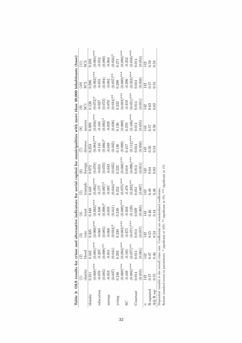
Tab

le3:

OLS

resu

lts

for

crim

ean

dal

tern

ativ

ein

dic

ator

sfo

rso

cial

capital

for

munic

ipal

itie

sw

ith

mor

eth

an30

,000

inhab

itan

ts(b

ase)

(1)

(2)

(3)

(4)

(5)

(6)

(7)

(8)

(9)

(10)

(11)

char

ity

bloo

dvo

tetr

ust

trus

tplc

fore

ign

divo

rce

mov

ers

SC1

SC2

SC3

dens

ity

0.21

10.

442

0.32

50.

448

0.44

30.

072

0.25

30.

393

0.13

90.

286

0.23

3(0

.068

)***

(0.0

61)*

**(0

.060

)***

(0.0

63)*

**(0

.062

)***

(0.0

78)

(0.0

84)*

**(0

.056

)***

(0.0

72)*

(0.0

62)*

**(0

.064

)***

educ

atio

n-0

.076

-0.2

07-0

.065

-0.1

66-0

.177

-0.0

51-0

.145

-0.1

65-0

.027

-0.0

55-0

.052

(0.0

85)

(0.0

98)*

*(0

.085

)(0

.098

)*(0

.097

)*(0

.070

)(0

.086

)*(0

.092

)*(0

.072

)(0

.084

)(0

.080

)un

emp

-0.0

53-0

.051

-0.0

60-0

.059

-0.0

87-0

.043

-0.0

49-0

.029

-0.0

70-0

.082

-0.0

64(0

.037

)(0

.041

)(0

.034

)*(0

.041

)(0

.044

)**

(0.0

35)

(0.0

35)

(0.0

38)

(0.0

34)*

*(0

.037

)**

(0.0

34)*

youn

g0.

246

0.29

20.

230

0.24

90.

252

0.22

20.

136

0.13

00.

232

0.29

90.

271

(0.0

69)*

**(0

.094

)***

(0.0

82)*

**(0

.080

)***

(0.0

75)*

**(0

.080

)***

(0.0

99)

(0.0

89)

(0.0

83)*

**(0

.080

)***

(0.0

80)*

**SC

-0.4

49-0

.165

-0.3

71-0

.203

-0.4

780.

618

0.41

70.

370

-0.3

19-0

.290

-0.3

52(0

.094

)***

(0.0

77)*

*(0

.071

)***

(0.1

29)

(0.2

02)*

*(0

.096

)***

(0.1

12)*

**(0

.106

)***

(0.0

51)*

**(0

.053

)***

(0.0

58)*

**C

onst

ant

0.01

40.

014

0.01

40.

029

0.05

10.

014

0.01

40.

014

0.01

40.

014

0.01

4(0

.055

)(0

.061

)(0

.057

)(0

.065

)(0

.067

)(0

.051

)(0

.056

)(0

.055

)(0

.051

)(0

.056

)(0

.054

)n

142

142

142

142

142

142

142

142

142

142

142

R-s

quar

ed0.

570.

470.

550.

460.

480.

640.

560.

570.

630.

570.

59A

djR

sqr

0.55

0.46

0.53

0.44

0.46

0.62

0.54

0.56

0.62

0.55

0.58

Dep

enden

tva

riable

isth

eov

erall

crim

era

te.

Coeffi

cien

tsare

standard

ized

coeffi

cien

ts.

Robust

standard

erro

rsin

pare

nth

eses

.*

signifi

cant

at

10%

;**

signifi

cant

at

5%

;***

signifi

cant

at

1%

.

32

Tab

le4:

OLS

resu

lts

for

crim

ean

dal

tern

ativ

ein

dic

ator

sfo

rso

cial

capital

for

munic

ipal

itie

sw

ith

mor

eth

an30

,000

inhab

itan

ts(e

xte

nded

)(1

)(2

)(3

)(4

)(5

)(6

)(7

)(8

)(9

)(1

0)(1

1)ch

arity

bloo

dvo

tetr

ust

trus

tplc

fore

ign

divo

rce

mov

ers

SC1

SC2

SC3

dens

ity

0.20

30.

370

0.26

30.

363

0.36

60.

063

0.28

00.

340

0.12

40.

225

0.19

7(0

.067

)***

(0.0

59)*

**(0

.062

)***

(0.0

63)*

**(0

.059

)***

(0.0

71)

(0.0

75)*

**(0

.058

)***

(0.0

69)*

(0.0

63)*

**(0

.063

)***

educ

atio

n-0

.047

-0.1

27-0

.051

-0.0

86-0

.096

-0.0

36-0

.107

-0.1

12-0

.025

-0.0

28-0

.039

(0.0

64)

(0.0

69)*

(0.0

61)

(0.0

71)

(0.0

68)

(0.0

53)

(0.0

66)

(0.0

73)

(0.0

56)

(0.0

62)

(0.0

59)

unem

p-0

.025

-0.0

21-0

.029

-0.0

30-0

.061

-0.0

21-0

.020

-0.0

13-0

.043

-0.0

50-0

.035

(0.0

33)

(0.0

35)

(0.0

32)

(0.0

33)

(0.0

36)*

(0.0

34)

(0.0

33)

(0.0

34)

(0.0

33)

(0.0

33)

(0.0

33)

youn

g0.

098

0.11

40.

095

0.07

20.

073

0.10

60.

029

0.03

10.

118

0.14

50.

132

(0.0

80)

(0.0

95)

(0.0

88)

(0.0

86)

(0.0

79)

(0.0

85)

(0.0

97)

(0.0

92)

(0.0

91)

(0.0

88)

(0.0

88)

ineq

ualit

y-0

.030

-0.0

990.

068

-0.0

65-0

.081

0.01

6-0

.058

-0.0

440.

045

0.02

80.

038

(0.0

55)

(0.0

57)*

(0.0

60)

(0.0

56)

(0.0

57)

(0.0

52)

(0.0

58)

(0.0

55)

(0.0

54)

(0.0

54)

(0.0

55)

shop

0.11

70.

146

0.14

80.

147

0.13

30.

178

0.09

20.

146

0.14

50.

165

0.14

3(0

.056

)**

(0.0

58)*

*(0

.054

)***

(0.0

62)*

*(0

.058

)**

(0.0

52)*

**(0

.057

)(0

.060

)**

(0.0

53)*

**(0

.057

)***

(0.0

54)*

**re

crat

0.13

60.

178

0.17

70.

163

0.17

60.

139

0.15

50.

112

0.13

50.

146

0.15

4(0

.062

)**

(0.0

67)*

**(0

.065

)***

(0.0

71)*

*(0

.065

)***

(0.0

56)*

*(0

.059

)***

(0.0

58)*

(0.0

56)*

*(0

.063

)**

(0.0

62)*

*co

fsho

p0.

244

0.24

80.

241

0.28

20.

280

0.14

70.

216

0.20

10.

190

0.24

50.

226

(0.0

69)*

**(0

.063

)***

(0.0

68)*

**(0

.070

)***

(0.0

66)*

**(0

.055

)***

(0.0

68)*

**(0

.081

)**

(0.0

60)*

**(0

.064

)***

(0.0

65)*

**SC

-0.3

31-0

.170

-0.3

17-0

.206

-0.5

180.

514

0.25

20.

236

-0.2

60-0

.240

-0.2

86(0

.090

)***

(0.0

73)*

*(0

.070

)***

(0.1

21)*

(0.1

81)*

**(0

.089

)***

(0.0

97)*

*(0

.090

)***

(0.0

47)*

**(0

.049

)***

(0.0

55)*

**C

onst

ant

0.01

40.

014

0.01

40.

029

0.05

40.

014

0.01

40.

014

0.01

40.

014

0.01

4(0

.050

)(0

.052

)(0

.050

)(0

.055

)(0

.056

)(0

.046

)(0

.051

)(0

.051

)(0

.047

)(0

.049

)(0

.048

)n

142

142

142

142

142

142

142

142

142

142

142

R-s

quar

ed0.

670.

630.

660.

620.

640.

710.

640.

650.

70.

670.

68A

djR

sqr

0.64

0.61

0.63

0.59

0.62

0.69

0.62

0.62

0.68

0.65

0.66

Dep

enden

tva

riable

isth

eov

erall

crim

era

te.

Coeffi

cien

tsare

standard

ized

coeffi

cien

ts.

Robust

standard

erro

rsin

pare

nth

eses

.*

signifi

cant

at

10%

;**

signifi

cant

at

5%

;***

signifi

cant

at

1%

.

33

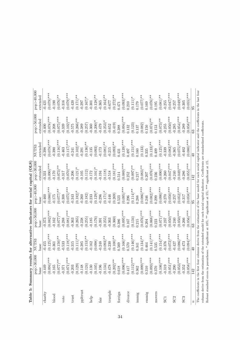
Tab

le5:

Sum

mar

yre

sult

sfo

ral

tern

ativ

ein

dic

ator

sfo

rso

cial

capit

al(O

LS)

pop>

30,0

00N

UT

S3po

p>50

,000

pop>

40,0

00po

p>30

,000

NU

TS3

pop>

50,0

00po

p>40

,000

base

base

base

base

exte

nded

exte

nded

exte

nded

exte

nded

char

ity

-0.4

49-0

.455

-0.3

73-0

.460

-0.3

31-0

.398

-0.4

00-0

.421

(0.0

94)*

**(0

.125

)***

(0.0

82)*

**(0

.080

)***

(0.0

90)*

**(0

.078

)***

(0.0

78)*

**(0

.079

)***

bloo

d-0

.165

-0.3

61-0

.162

-0.1

75-0

.170

-0.3

90-0

.208

-0.1

90(0

.077

)**

(0.1

50)*

*(0

.077

)**

(0.0

77)*

*(0

.073

)**

(0.1

16)*

**(0

.075

)***

(0.0

76)*

*vo

te-0

.371

-0.5

33-0

.288

-0.3

08-0

.317

-0.4

63-0

.339

-0.3

16(0

.071

)***

(0.1

18)*

**(0

.081

)***

(0.0

75)*

**(0

.070

)***

(0.1

17)*

**(0

.102

)***

(0.0

79)*

**tr

ust

-0.2

03-0

.315

-0.3

63-0

.343

-0.2

06-0

.241

-0.5

75-0

.420

(0.1

29)

(0.1

11)*

**(0

.265

)(0

.182

)*(0

.121

)*(0

.102

)**

(0.2

66)*

*(0

.171

)**

pplt

rust

-0.1

48-0

.385

-0.2

38-0

.260

-0.1

05-0

.291

-0.3

89-0

.297

(0.1

24)

(0.1

53)*

*(0

.255

)(0

.182

)(0

.112

)(0

.136

)**

(0.2

57)

(0.1

67)*

help

-0.1

30-0

.162

-0.1

85-0

.233

-0.1

72-0

.135

-0.3

60-0

.301

(0.1

05)

(0.0

98)

(0.1

76)

(0.1

29)*

(0.1

01)*

(0.0

93)

(0.2

00)*

(0.1

28)*

*fa

ir-0

.196

-0.2

48-0

.391

-0.2

96-0

.194

-0.1

73-0

.479

-0.3

65(0

.134

)(0

.093

)**

(0.2

55)

(0.1

71)*

(0.1

18)

(0.0

81)*

*(0

.253

)*(0

.164

)**

trus

tplc

-0.4

78-0

.230

-0.3

63-0

.446

-0.5

18-0

.215

-0.6

52-0

.677

(0.2

02)*

*(0

.100

)**

(0.3

60)

(0.2

69)

(0.1

81)*

**(0

.093

)**

(0.4

19)

(0.2

72)*

*fo

reig

n0.

618

0.56

90.

386

0.52

30.

514

0.43

10.

388

0.47

1(0

.096

)***

(0.1

66)*

**(0

.095

)***

(0.0

95)*

**(0

.089

)***

(0.1

39)*

**(0

.094

)***

(0.0

93)*

**di

vorc

e0.

417

0.57

00.

167

0.29

60.

252

0.49

70.

132

0.21

0(0

.112

)***

(0.1

46)*

**(0

.134

)(0

.114

)**

(0.0

97)*

*(0

.151

)***

(0.1

23)

(0.1

11)*

imm

ig0.

362

0.34

10.

215

0.28

80.

217

0.16

00.

137

0.17

9(0

.099

)***

(0.1

34)*

*(0

.076

)***

(0.0

86)*

**(0

.083

)**

(0.1

33)

(0.0

82)

(0.0

77)*

*em

mig

0.31

00.

464

0.20

40.

246

0.20

70.

335

0.15

00.

169

(0.0

93)*

**(0

.141

)***

(0.0

68)*

**(0

.082

)***

(0.0

76)*

**(0

.133

)**

(0.0

74)*

*(0

.076

)**

mov

ers

0.37

00.

535

0.22

30.

299

0.23

60.

409

0.15

30.

195

(0.1

06)*

**(0

.154

)***

(0.0

71)*

**(0

.090

)***

(0.0

90)*

**(0

.125

)***

(0.0

73)*

*(0

.081

)**

SC1

-0.3

19-0

.376

-0.2

37-0

.270

-0.2

60-0

.339

-0.2

55-0

.255

(0.0

51)*

**(0

.072

)***

(0.0

50)*

**(0

.050

)***

(0.0

47)*

**(0

.083

)***

(0.0

50)*

**(0

.047

)***

SC2

-0.2

90-0

.427

-0.2

40-0

.257

-0.2

40-0

.365

-0.2

85-0

.257

(0.0

53)*

**(0

.086

)***

(0.0

50)*

**(0

.052

)***

(0.0

49)*

**(0

.075

)***

(0.0

54)*

**(0

.049

)***

SC3

-0.3

52-0

.473

-0.2

66-0

.317

-0.2

86-0

.402

-0.2

89-0

.305

(0.0

58)*

**(0

.094

)***

(0.0

56)*

**(0

.058

)***

(0.0

55)*

**(0

.080

)***

(0.0

58)*

**(0

.055

)***

n14

240

6395

142

4063

95T

he

coeffi

cien

tsin

the

firs

tfo

ur

colu

mns

der

ive

from

the

esti

mati

on

ofth

ebase

model

for

each

soci

alca

pit

alin

dic

ato

rand

the

coeffi

cien

tsin

the

last

four

colu

mn

der

ive

from

the

esti

mati

on

ofth

eex

tended

model

for

each

soci

alca

pit

alin

dic

ato

r.C

oeffi

cien

tsare

standard

ized

coeffi

cien

ts.

Robust

standard

erro

rsin

pare

nth

eses

.*

signifi

cant

at

10%

;**

signifi

cant

at

5%

;***

signifi

cant

at

1%

.

34

Table 6: 2SLS results for crime and social capital for municipalities with more than 30,000 inhabitants(1) 1st stage (2) 2SLS (3) 1st stage (4) 2SLS (5) 1st stage (6) 2SLSSC1 crime SC2 crime SC3 crime

density -0.841 0.089 -0.511 0.167 -0.524 0.162(0.133)*** (0.086) (0.111)*** (0.072)** (0.098)*** (0.074)**

education 0.294 -0.013 0.314 0.003 0.230 -0.025(0.091)*** (0.048) (0.077)*** (0.057) (0.073)*** (0.053)

unemp -0.085 -0.048 -0.129 -0.065 -0.059 -0.039(0.060) (0.035) (0.063)** (0.036)* (0.048) (0.035)

young 0.134 0.128 0.279 0.182 0.167 0.149(0.127) (0.089) (0.099)*** (0.091)** (0.093)* (0.086)*

inequality 0.318 0.063 0.314 0.069 0.301 0.062(0.104)*** (0.061) (0.099)*** (0.063) (0.080)*** (0.062)

shop 0.024 0.148 0.121 0.180 0.030 0.146(0.095) (0.051)*** (0.097) (0.056)*** (0.076) (0.053)***

recrat -0.026 0.129 -0.001 0.135 0.045 0.149(0.111) (0.056)** (0.081) (0.063)** (0.072) (0.061)**

cofshop -0.330 0.179 -0.130 0.235 -0.188 0.217(0.097)*** (0.062)*** (0.077)* (0.062)*** (0.064)*** (0.064)***

foreign1859 -0.366 -0.309 -0.237(0.090)*** (0.085)*** (0.066)***

protestant1859 0.315 0.321 0.396(0.086)*** (0.087)*** (0.067)***

#school1859 0.185 0.172 0.106(0.093)** (0.082)** (0.079)

SC1 -0.295(0.076)***

SC2 -0.328(0.081)***

SC3 -0.341(0.081)***

Constant 0.000 0.014 0.000 0.014 0.000 0.014(0.088) (0.046) (0.080) (0.048) (0.069) (0.047)

n 142 142 142 142 142 142Adj R sqr 0.66 0.68 0.53 0.64 0.61 0.66R-squared 0.69 0.57 0.64F-test instrm. 16.18*** 17.43*** 25.16***overid 4.41 (0.11) 3.28 (0.19) 2.11 (0.34)Dependent variable is the overall crime rate. All variables are standardized. Columns 1, 3 and 5 are the first stage results.

Robust standard errors in parentheses. * significant at 10%; ** significant at 5%; *** significant at 1%.

F-test is a test of joint significance of the instruments.

overid is a test of over identification. Null hypothesis: Over-identifying restrictions are valid.

35

Tab

le7:

Diff

eren

tso

cial

capit

alin

dic

ator

sin

the

2SLS

spec

ifica

tion

pop>

40,0

00(b

ase)

pop>

30,0

00(b

ase)

pop>

40,0

00(e

xten

ded)

pop>

30,0

00(e

xten

ded)

2SLS

F-t

est

2SLS

F-t

est

2SLS

F-t

est

2SLS

F-t

est

SC1

-0.3

2320

.75*

**-0

.321

28.9

2***

-0.2

8817

.73*

**-0

.295

16.1

8***

(0.0

84)*

**(0

.074

)***

(0.0

73)*

**(0

.076

)***

SC2

-0.4

0919

.11*

**-0

.375

27.6

1***

-0.3

4017

.55*

**-0

.328

17.4

3***

(0.0

98)*

**(0

.083

)***

(0.0

81)*

**(0

.081

)***

SC3

-0.4

5322

.32*

**-0

.393

32.5

4***

-0.3

8320

.88*

**-0

.341

25.1

6***

(0.0

99)*

**(0

.081

)***

(0.0

85)*

**(0

.081

)***

char

ity

-0.9

007.

65**

*-0

.776

10.2

7***

-0.7

446.

71**

*-0

.684

8.23

***

(0.2

24)*

**(0

.182

)***

(0.1

97)*

**(0

.191

)***

bloo

d-1

.166

4.25

***

-1.3

753.

52**

-0.8

783.

42**

-0.8

213.

03**

(0.3

54)*

**(0

.451

)***

(0.2

74)*

**(0

.263

)***

vote

-0.4

8732

.15*

**-0

.432

44.8

6***

-0.4

5631

.37*

**-0

.387

38.8

0***

(0.1

33)*

**(0

.101

)***

(0.1

22)*

**(0

.101

)***

fore

ign

0.59

112

.50*

**0.

632

16.6

4***

0.52

47.

89**

*0.

543

7.84

***

(0.2

16)*

**(0

.188

)***

(0.2

04)*

*(0

.190

)***

divo

rce

0.57

69.

35**

*0.

878

6.91

***

0.48

66.

07**

*0.

777

2.61

*(0

.208

)***

(0.2

71)*

**(0

.214

)**

(0.3

67)*

*R

obust

standard

erro

rsin

pare

nth

eses

.*

signifi

cant

at

10%

;**

signifi

cant

at

5%

;***

signifi

cant

at

1%

.

All

coeffi

cien

tsare

obta

ined

from

the

2SLS

model

(equati

on

4)

when

itis

esti

mate

dw

ith

diff

eren

tso

cialca

pit

alin

dic

ato

rs.

For

each

subsa

mple

and

model

the

firs

tco

lum

npre

sents

the

2SLS

coeffi

cien

tsfo

rdiff

eren

tso

cialca

pit

alin

dic

ato

rs.

The

seco

nd

colu

mn

pre

sents

the

F-t

est.

More

det

ailed

resu

lts

are

available

from

the

auth

ors

upon

reques

t.

36

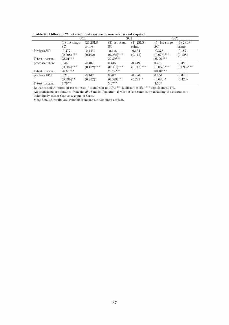
Table 8: Different 2SLS specifications for crime and social capitalSC1 SC2 SC3

(1) 1st stage (2) 2SLS (3) 1st stage (4) 2SLS (5) 1st stage (6) 2SLSSC crime SC crime SC crime

foreign1859 -0.472 -0.145 -0.418 -0.164 -0.378 -0.182(0.098)*** (0.102) (0.088)*** (0.115) (0.075)*** (0.128)

F-test instrm. 23.01*** 22.59*** 25.26***protestant1859 0.450 -0.407 0.436 -0.419 0.481 -0.380

(0.084)*** (0.102)*** (0.081)*** (0.112)*** (0.062)*** (0.093)***F-test instrm. 28.63*** 28.74*** 60.40***#school1859 0.216 -0.467 0.207 -0.486 0.156 -0.646

(0.099)** (0.262)* (0.089)** (0.283)* (0.086)* (0.420)F-test instrm. 4.76** 5.37** 3.30*Robust standard errors in parentheses. * significant at 10%; ** significant at 5%; *** significant at 1%.

All coefficients are obtained from the 2SLS model (equation 4) when it is estimated by including the instruments

individually rather than as a group of three.

More detailed results are available from the authors upon request.

37

Tab

le9:

Sum

mar

yre

sult

sfo

rcr

ime

cate

gori

esan

din

dic

ator

sof

soci

alca

pital

for

munic

ipal

itie

sw

ith

mor

eth

an30

,000

inhab

itan

tsn=

142

char

ity

bloo

dvo

tetr

ust

trus

tplc

fore

ign

divo

rce

mov

ers

SCSC

1SC

2ex

pec

ted

sign

(-)

(-)

(-)

(-)

(-)

(+)

(+)

(+)

(-)

(-)

(-)

crim

e**

***

***

***

***

***

***

***

***

***

hom

icid

e*

***

***

***

**as

saul

t**

***

***

***

***

***

***

***

***

***

***

rape

***

***

***

***

***

****

***

***

*ro

bber

y**

***

***

****

***

***

***

***

*th

eft

***

***

***

****

***

***

***

*au

toth

eft

***

***

***

**

****

***

***

*bu

rgla

ry**

***

****

***

***

***

*dr

ug**

***

***

****

**

****

***

***

*T

he

signifi

cance

level

sder

ive

from

esti

mati

on

ofth

eex

tended

model

(equati

on

3)

for

each

crim

eca

tegory

and

each

soci

alca

pit

alin

dic

ato

r.

Robust

standard

erro

rsin

pare

nth

eses

.*

signifi

cant

at

10%

;**

signifi

cant

at

5%

;***

signifi

cant

at

1%

.

38

Tab

le10

:A

lter

nat

ive

spec

ifica

tion

sto

expla

incr

ime

diff

eren

tial

sSC

1SC

2SC

3fo

reig

n18

59pr

ot18

59ed

uc18

59fo

reig

ndi

vorc

eO

rigi

nalco

effici

ents

of(1

)O

LS

-0.2

60-0

.240

-0.2

86O

LS

and

2SLS

(0.0

47)*

**(0

.049

)***

(0.0

55)*

**es

tim

atio

ns(2

)2S

LS

-0.2

95-0

.328

-0.3

41(0

.076

)***

(0.0

81)*

**(0

.081

)***

Whe

ndi

vorc

ean

d(3

)O

LS

-0.1

440.

400

-0.0

29fo

reig

nar

ein

clud

ed(0

.064

)**

(0.1

05)*

**(0

.095

)as

inde

pend

ent

(4)

2SLS

-0.2

270.

345

-0.0

66va

riab

les

(0.1

21)*

(0.1

34)*

**(0

.096

)W

hen

hist

oric

al(5

)O

LS

-0.2

49-0

.081

-0.0

92-0

.029

vari

able

sar

e(0

.055

)***

(0.0

58)

(0.0

51)*

(0.0

54)

incl

uded

as(6

)O

LS

-0.2

13-0

.056

-0.1

02-0

.039

inde

pend

ent

vari

able

s(0

.057

)***

(0.0

57)

(0.0

52)*

(0.0

56)

(7)

OLS

-0.2

63-0

.053

-0.0

67-0

.047

(0.0

67)*

**(0

.056

)(0

.055

)(0

.056

)W

hen

the

mos

tin

fluen

tial

(8)

OLS

-0.2

39-0

.229

-0.2

69ob

serv

atio

nis

rem

oved

(0.0

45)*

**(0

.047

)***

(0.0

53)*

**(a

ccor

ding

toC

ook’

sD

)(9

)2S

LS

-0.2

99-0

.336

-0.3

49(0

.076

)***

(0.0

80)*

**(0

.080

)***

Whe

nth

efir

stfiv

em

ost

(10)

OLS

-0.2

40-0

.223

-0.2

63in

fluen

tial

obse

rvat

ions

(0.0

43)*

**(0

.045

)***

(0.0

50)*

**ar

ere

mov

ed(1

1)2S

LS

-0.2

88-0

.329

-0.3

39(a

ccor

ding

toC

ook’

sD

)(0

.072

)***

(0.0

78)*

**(0

.078

)***

Whe

nth

em

ost

influ

enti

al(1

2)O

LS

-0.2

40-0

.220

-0.2

68ob

serv

atio

nis

rem

oved

(0.0

44)*

**(0

.045

)***

(0.0

53)*

**(a

ccor

ding

toD

FB

etas

)(1

3)2S

LS

-0.3

00-0

.333

-0.3

48(0

.075

)***

(0.0

79)*

**(0

.079

)***

Whe

nth

efir

stfiv

em

ost

(14)

OLS

-0.2

36-0

.220

-0.2

75in

fluen

tial

obse

rvat

ions

(0.0

43)*

**(0

.043

)***

(0.0

47)*

**ar

ere

mov

ed(1

5)2S

LS

-0.3

24-0

.358

-0.3

77(a

ccor

ding

toD

FB

etas

)(0

.081

)***

(0.0

85)*

**(0

.082

)***

The

signifi

cance

level

sder

ive

from

the

esti

mati

ons

ofdiff

eren

tsp

ecifi

cati

ons

ofth

eex

tended

model

(equati

on

3).

Dep

enden

tva

riable

isth

eov

erall

crim

era

te.

Robust

standard

erro

rsin

pare

nth

eses

.*

signifi

cant

at

10%

;**

signifi

cant

at

5%

;***

signifi

cant

at

1%

.

39

-3-2-1012Voter turnout

-2-1

01

23

Volu

ntar

y co

ntrib

utio

ns-2-10123

Blood donations-2

-10

12

3Vo

lunt

ary

cont

ribut

ions

-2-10123Percentage of foreigners

-2-1

01

23

Volu

ntar

y co

ntrib

utio

ns

-3-2-1012Divorce rate

-2-1

01

23

Volu

ntar

y co

ntrib

utio

ns

-2-10123Blood donations

-3-2

-10

12

Vot

er tu

rnou

t

-2-10123Percentage of foreigners

-3-2

-10

12

Vote

r tur

nout

-3-2-1012Divorce rates

-3-2

-10

12

Vote

r tur

nout

-2-10123Percentage of foreigners

-2-1

01

23

Bloo

d do

natio

ns

-3-2-1012Divorce rates

-2-1

01

23

Bloo

d do

natio

ns

-2-10123Percentage of foreigners

-3-2

-10

12

Div

orce

rate

s

Fig

ure

1:Sc

atte

rplo

tsof

soci

alca

pita

lin

dica

tors

for

142

mun

icip

alit

ies

wit

hm

ore

than

30,0

00in

habi

tant

s

40

-2-10123overall crime

-20

24

volu

ntar

y co

ntrib

utio

nsco

ef =

-.44

9, (

robu

st) s

e =

.094

, t =

-4.7

88

-2-10123overall crime

-20

24

6bl

ood

dona

tions

coef

= -.

165,

(rob

ust)

se =

.077

, t =

-2.1

57

-2-10123overall crime

-2-1

01

2vo

ter t

urno

utco

ef =

-.3

71, (

robu

st) s

e =

.071

, t =

-5.1

98

-2-10123overall crime

-1-.5

0.5

1ge

nera

lized

trus

tco

ef =

-.20

3, (

robu

st) s

e =

.129

, t =

-1.5

68

-2-10123overall crime

-2-1

01

23

perc

enta

ge o

f for

eign

ers

coef

= .6

18, (

robu

st) s

e =

.096

, t =

6.4

55

-2-10123overall crime

-2-1

01

2di

vorc

e ra

tes

coef

= .4

17, (

robu

st) s

e =

.112

, t =

3.7

38

Not

e: A

dded

-var

iabl

e pl

ots

are

from

OLS

regr

essi

ons

of c

rime

on a

con

stan

t, po

pula

tion

dens

ity, %

of y

oung

, edu

catio

n, u

nem

ploy

men

t and

a s

ocia

l cap

ital i

ndic

ator

.

Fig

ure

2:O

vera

llcr

ime

and

soci

alca

pita

lin

dica

tors

for

142

mun

icip

alit

ies

wit

hm

ore

than

30,0

00in

habi

tant

s

41

-2-10123overall crime

-4-2

02

4so

cial

cap

ital i

ndex

coef

= -

.319

, (ro

bust

) se

= .0

51, t

= -6

.268

02468murder

-4-2

02

4so

cial

cap

ital i

ndex

coef

= -.

194,

(ro

bust

) se

= .0

97, t

= -2

.009

-2024assault

-4-2

02

4so

cial

cap

ital i

ndex

coef

= -

.431

, (ro

bust

) se

= .0

51, t

= -8

.403

-10123rape

-4-2

02

4so

cial

cap

ital i

ndex

coef

= -.

356,

(ro

bust

) se

= .0

56, t

= -6

.378

-20246robbery

-4-2

02

4so

cial

cap

ital in

dex

coef

= -

.307

, (ro

bust

) se

= .0

8, t

= -3

.846

-20246theft

-4-2

02

4so

cial

cap

ital i

ndex

coef

= -.

257,

(ro

bust

) se

= .0

47, t

= -5

.425

-20246car theft

-4-2

02

4so

cial

cap

ital i

ndex

coef

= -

.229

, (ro

bust

) se

= .0

55, t

= -4

.146

-2024drug crimes

-4-2

02

4so

cial

cap

ital i

ndex

coef

= -.

271,

(ro

bust

) se

= .0

53, t

= -5

.157

Not

e: A

dded

-var

iabl

e pl

ots

are

from

OLS

regr

essi

ons

of c

rime

type

s on

a c

onst

ant,

popu

latio

n de

nsity

, % o

f you

ng, e

duca

tion,

une

mpl

oym

ent a

nd s

ocia

l cap

ital i

ndex

.

Fig

ure

3:C

rim

eca

tego

ries

and

soci

alca

pita

lfo

r14

2m

unic

ipal

itie

sw

ith

mor

eth

an30

,000

inha

bita

nts

42

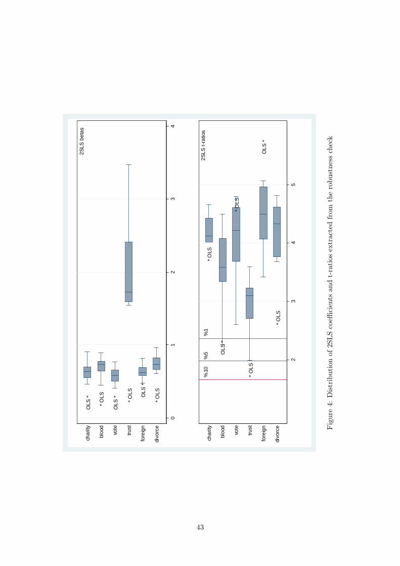
OLS

*

* OLS

OLS

* * OLS OLS

*

* OLS

2SLS

bet

as

01

23

4

divo

rce

fore

ign

trust

vote

bloo

d

char

ity

* OLS

OLS

*

* OLS

* O

LS

OLS

*

* OLS

%10

%5

%1

2SLS

t-ra

tios

23

45

divo

rce

fore

ign

trust

vote

bloo

d

char

ity

Fig

ure

4:D

istr

ibut

ion

of2S

LS

coeffi

cien

tsan

dt-

rati

osex

trac

ted

from

the

robu

stne

ssch

eck

43

inco

me_

gap

inco

me_

gap

inco

me_

nw

inco

me_

nw

inco

me_

nw

inco

me_

w

inco

me_

w

inco

me_

w

inco

me_

pinco

me_

p

inco

me_

t

inco

me_

t

inco

me_

t

orig

inal

orig

inal

orig

inal

inco

me_

gap

inco

me_

p

0.00

0.05

0.10

0.15

0.20

0.25

0.30

0.35

SC

1

SC

2

SC

3

Fig

ure

5:St

anda

rdiz

edco

effici

ents

ofSC

whe

nco

ntro

lled

for

diffe

rent

indi

cato

rsof

inco

me

44

0.00

0.01

0.02

0.03

0.04

0.05

0.06

0.07

assa

ult

robb

ery

thef

t

carth

eft

burg

lary

dom

estic

bur

glar

y

drug

nonw

est

wes

t

fore

ign

Fig

ure

6:O

rigi

nof

fore

igne

rsan

ddi

ffere

nces

incr

ime

rate

s

45

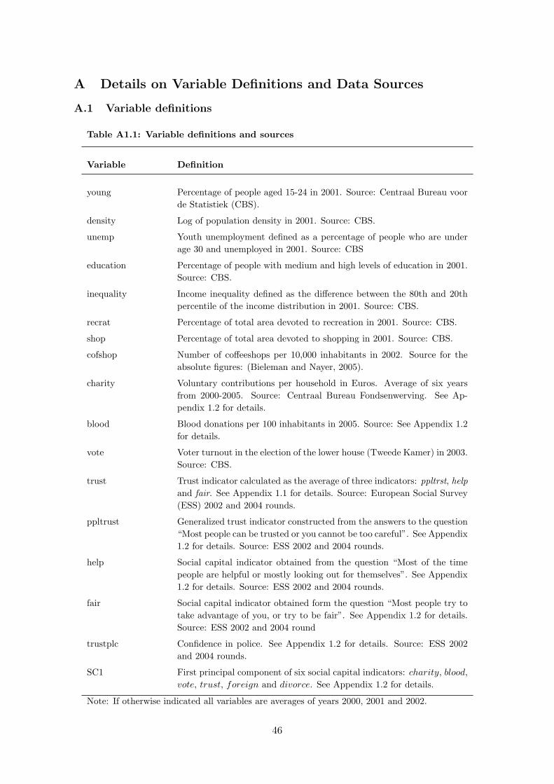
A Details on Variable Definitions and Data Sources

A.1 Variable definitions

Table A1.1: Variable definitions and sources

Variable Definition

young Percentage of people aged 15-24 in 2001. Source: Centraal Bureau voorde Statistiek (CBS).

density Log of population density in 2001. Source: CBS.

unemp Youth unemployment defined as a percentage of people who are underage 30 and unemployed in 2001. Source: CBS

education Percentage of people with medium and high levels of education in 2001.Source: CBS.

inequality Income inequality defined as the difference between the 80th and 20thpercentile of the income distribution in 2001. Source: CBS.

recrat Percentage of total area devoted to recreation in 2001. Source: CBS.

shop Percentage of total area devoted to shopping in 2001. Source: CBS.

cofshop Number of coffeeshops per 10,000 inhabitants in 2002. Source for theabsolute figures: (Bieleman and Nayer, 2005).

charity Voluntary contributions per household in Euros. Average of six yearsfrom 2000-2005. Source: Centraal Bureau Fondsenwerving. See Ap-pendix 1.2 for details.

blood Blood donations per 100 inhabitants in 2005. Source: See Appendix 1.2for details.

vote Voter turnout in the election of the lower house (Tweede Kamer) in 2003.Source: CBS.

trust Trust indicator calculated as the average of three indicators: ppltrst, helpand fair. See Appendix 1.1 for details. Source: European Social Survey(ESS) 2002 and 2004 rounds.

ppltrust Generalized trust indicator constructed from the answers to the question“Most people can be trusted or you cannot be too careful”. See Appendix1.2 for details. Source: ESS 2002 and 2004 rounds.

help Social capital indicator obtained from the question “Most of the timepeople are helpful or mostly looking out for themselves”. See Appendix1.2 for details. Source: ESS 2002 and 2004 rounds.

fair Social capital indicator obtained form the question “Most people try totake advantage of you, or try to be fair”. See Appendix 1.2 for details.Source: ESS 2002 and 2004 round

trustplc Confidence in police. See Appendix 1.2 for details. Source: ESS 2002and 2004 rounds.

SC1 First principal component of six social capital indicators: charity, blood,vote, trust, foreign and divorce. See Appendix 1.2 for details.

Note: If otherwise indicated all variables are averages of years 2000, 2001 and 2002.

46

Variable Definition

SC2 First principal component of four social capital indicators: charity,blood, vote and trust. See Appendix 1.2 for details.

SC3 First principal component of three social capital indicators: charity,blood and vote. See Appendix 1.2 for details.

divorce Percentage of divorces in the total population. Source: CBS.

immig Immigration as a percentage of the total population. Source: CBS.

emmig Emigration as a percentage of the total population. Source: CBS.

movers Sum of immigration and emigration as a percentage of the total popu-lation. Source: CBS.

foreign Percentage of foreigners in the total population. Source: CBS.

foreign1859 Percentage of foreigners in the total population in 1859. See Appendix1.3 for details. Source: Volkstellingen Archief.

protestant1859 Percentage of Protestants in the total population in 1859. See Appendix1.3 for details. Source: Volkstellingen Archief.

#school1859 Number of schools per 100 inhabitants in 1859. See Appendix 1.3 fordetails. Source: Volkstellingen Archief.

crime Crime rates including all recorded crimes in 2002. See Appendix 1.4 fordetailed information on crime data and how crime categories are formed.

homicide Homicide per 100 inhabitants in 2002.

assault Assault per 100 inhabitants in 2002.

rape Rape per 100 inhabitants in 2002.

robbery Robbery per 100 inhabitants in 2002.

theft Theft per 100 inhabitants in 2002.

autotheft Motor vehicle theft per 100 inhabitants in 2002.

burglary Burglary per 100 inhabitants in 2002.

domestic burglary Domestic burglary per 100 inhabitants in 2002.

drug Crime related to hard drugs per 100 inhabitants in 2002.

Note: If otherwise indicated all variables are averages of years 2000, 2001 and 2002.

47

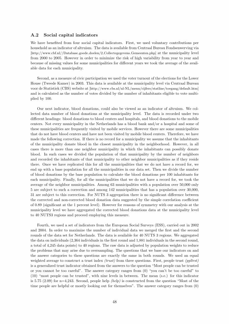
A.2 Social capital indicators

We have benefited from four social capital indicators. First, we used voluntary contributions perhousehold as an indicator of altruism. The data is available from Centraal Bureau Fondsenwerving via[http://www.cbf.nl//Database goede doelen/2 Collectegegevens Gemeenten.php] at the municipality levelfrom 2000 to 2005. However in order to minimize the risk of high variability from year to year andbecause of missing values for some municipalities for different years we took the average of the avail-able data for each municipality.

Second, as a measure of civic participation we used the voter turnout of the elections for the LowerHouse (Tweede Kamer) in 2003. This data is available at the municipality level via Centraal Bureauvoor de Statistiek (CBS) website at [http://www.cbs.nl/nl-NL/menu/cijfers/statline/toegang/default.htm]

and is calculated as the number of votes divided by the number of inhabitants eligible to vote multi-plied by 100.

Our next indicator, blood donations, could also be viewed as an indicator of altruism. We col-lected data number of blood donations at the municipality level. The data is recorded under twodifferent headings: blood donations to blood centers and hospitals, and blood donations to the mobilecenters. Not every municipality in the Netherlands has a blood bank and/or a hospital and some ofthese municipalities are frequently visited by mobile services. However there are some municipalitiesthat do not have blood centers and have not been visited by mobile blood centers. Therefore, we havemade the following correction. If there is no record for a municipality we assume that the inhabitantsof the municipality donate blood in the closest municipality in the neighborhood. However, in allcases there is more than one neighbor municipality in which the inhabitants can possibly donateblood. In such cases we divided the population of that municipality by the number of neighborsand recorded the inhabitants of that municipality to other neighbor municipalities as if they residethere. Once we have replicated this for all the municipalities that we do not have a record for, weend up with a base population for all the municipalities in our data set. Then we divide the numberof blood donations by the base population to calculate the blood donations per 100 inhabitants foreach municipality. Finally, for all the municipalities that we do not have a record for, we took theaverage of the neighbor municipalities. Among 63 municipalities with a population over 50,000 only5 are subject to such a correction and among 142 municipalities that has a population over 30,000,31 are subject to this correction. For NUTS 3 aggregation there is no significant difference betweenthe corrected and non-corrected blood donation data suggested by the simple correlation coefficientof 0.89 (significant at the 1 percent level). However for reasons of symmetry with our analysis at themunicipality level we have aggregated the corrected blood donations data at the municipality levelto 40 NUTS3 regions and proceed employing this measure.

Fourth, we used a set of indicators from the European Social Surveys (ESS), carried out in 2002and 2004. In order to maximize the number of individual data we merged the first and the secondrounds of the data set for Netherlands. The data is available for 40 NUTS 3 regions. We aggregatedthe data on individuals (2,364 individuals in the first round and 1,881 individuals in the second round,a total of 4,245 data points) to 40 regions. The raw data is adjusted by population weights to reducethe problems that may arise due to oversampling. The questions that we base our indicators on andthe answer categories to these questions are exactly the same in both rounds. We used an equalweighted average to construct a trust index (trust) from three questions. First, people trust (ppltrst)is a generalized trust indicator obtained from the answers to the question “Most people can be trustedor you cannot be too careful”. The answer category ranges from (0) “you can’t be too careful” to(10) “most people can be trusted”, with nine levels in between. The mean (s.e.) for this indicatoris 5.75 (2.09) for n=4,243. Second, people help (help) is constructed from the question “Most of thetime people are helpful or mostly looking out for themselves”. The answer category ranges from (0)

48

“people mostly look out for themselves” to (10) “people mostly try to be helpful”, with nine levels inbetween. The mean (s.e.) for this indicator is 5.30 (1.97) for n=4,242. Third, people fair (fair) is anindicator obtained from the question “Most people try to take advantage of you, or try to be fair”.The answer category ranges from (0) “most people would try to take advantage of me” to (10) “mostpeople would try to be fair”, with nine levels in between. The mean (s.e.) for this indicator is 6.20(1.85) for n=4,233. The mean (s.e.) for the trust index is 5.75 (1.58) for n=4,229. We also used thequestion on confidence to police (trustplc) for robustness reasons. The question is “How much youpersonally trust in police”. The answer category ranges from (0) “no trust at all” to (10) “completetrust”. The mean (s.e.) for this indicator is 5.89 (1.94) for n=4,213. One particular weakness ofthese measures is that they are observed at the regional level and when conducting the analysis atthe municipality level these indicators have the same number for all the municipalities belonging tothe same NUTS3 definition.

In addition to these four indicators, we also used two other indicators − the percentage of di-vorces and the percentage of foreigners in the total population − as they display high and significantcorrelations with the above four indicators. Out of these seemingly unrelated indicators we haveconstructed several social capital indices by using principal component analysis (PCA). We first in-cluded 6 indicators, charity, blood, vote, trust, foreign and divorce, to form an all inclusive measureand labeled it as SC1. Then we included only four social capital indicators, excluding divorce andforeign and form SC2 defined as the first principal component of charity, blood, vote and trust.Finally we constructed a third index out of three indicators, charity, blood and vote, and labeledit SC3. The reason for this is that trust is measured at the regional level as discussed above andespecially in the analysis at the municipality level this might result in measurement error.

To check the robustness of our indices we constructed all possible combinations of these indicesby interchanging between indicators. For instance, we can use ppltrust, help, fair separately insteadof trust or we can use immig instead of foreign. All constructed indices behave in a similar way. Wealso did not include similar indicators in content (for instance, including ppltrust, help or trustplc

at the same time) because PCA tends to give similar weights to these indicators and the resultingindex becomes very powerful (i.e., the probability of obtaining a significant coefficient for the socialcapital index in regressions increases considerably).

Table A1.2 below displays information on the principal component loadings of the first princi-pal component and the explained variance for each social capital index for different samples. Asvisible from the table the indicators have positive loadings. On the contrary indicators that areassociated with the absence of social capital have negative loadings as expected. The PCA tendsto put more (and similar in terms of quantity) weight on charity, vote, foreign and divorce andless weight one blood and trust. One reason for this is that blood and trust involve data correctionsand interpolations. This can be easily seen from the table. For instance loadings to blood decreaseconsiderably in all three social capital indices as we move to the right of the table (i.e., the numberof corrected/interpolated data points increase as the sample size increases from 40 NUTS3 regionswith no data corrections to 142 municipalities with some data corrections, which seems to reducethe robustness of the indicator). After all this can be viewed as a positive outcome and it helps toproduce a social capital indicator by specifically placing less weight on some indicators. All indicesare expected to display a negative relationship with crime.

49

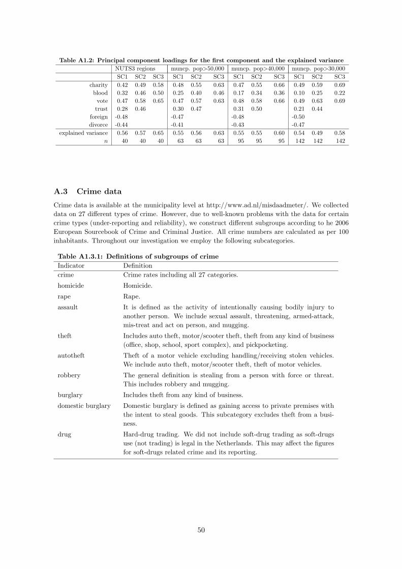
Table A1.2: Principal component loadings for the first component and the explained varianceNUTS3 regions muncp. pop>50,000 muncp. pop>40,000 muncp. pop>30,000SC1 SC2 SC3 SC1 SC2 SC3 SC1 SC2 SC3 SC1 SC2 SC3

charity 0.42 0.49 0.58 0.48 0.55 0.63 0.47 0.55 0.66 0.49 0.59 0.69blood 0.32 0.46 0.50 0.25 0.40 0.46 0.17 0.34 0.36 0.10 0.25 0.22vote 0.47 0.58 0.65 0.47 0.57 0.63 0.48 0.58 0.66 0.49 0.63 0.69trust 0.28 0.46 0.30 0.47 0.31 0.50 0.21 0.44

foreign -0.48 -0.47 -0.48 -0.50divorce -0.44 -0.41 -0.43 -0.47

explained variance 0.56 0.57 0.65 0.55 0.56 0.63 0.55 0.55 0.60 0.54 0.49 0.58n 40 40 40 63 63 63 95 95 95 142 142 142

A.3 Crime data

Crime data is available at the municipality level at http://www.ad.nl/misdaadmeter/. We collecteddata on 27 different types of crime. However, due to well-known problems with the data for certaincrime types (under-reporting and reliability), we construct different subgroups according to he 2006European Sourcebook of Crime and Criminal Justice. All crime numbers are calculated as per 100inhabitants. Throughout our investigation we employ the following subcategories.

Table A1.3.1: Definitions of subgroups of crimeIndicator Definitioncrime Crime rates including all 27 categories.

homicide Homicide.

rape Rape.

assault It is defined as the activity of intentionally causing bodily injury toanother person. We include sexual assault, threatening, armed-attack,mis-treat and act on person, and mugging.

theft Includes auto theft, motor/scooter theft, theft from any kind of business(office, shop, school, sport complex), and pickpocketing.

autotheft Theft of a motor vehicle excluding handling/receiving stolen vehicles.We include auto theft, motor/scooter theft, theft of motor vehicles.

robbery The general definition is stealing from a person with force or threat.This includes robbery and mugging.

burglary Includes theft from any kind of business.

domestic burglary Domestic burglary is defined as gaining access to private premises withthe intent to steal goods. This subcategory excludes theft from a busi-ness.

drug Hard-drug trading. We did not include soft-drug trading as soft-drugsuse (not trading) is legal in the Netherlands. This may affect the figuresfor soft-drugs related crime and its reporting.

50

Table A1.3.2: Distribution of criminal activity for different sampleslarge city pop>50,000 pop>40,000 pop>30,000

crime 52.57 70.41 77.04 83.19homicide 50.84 66.48 74.30 84.36rape 49.44 67.89 75.09 81.35assault 51.91 70.86 77.50 83.49robbery 76.82 90.13 93.26 94.97theft 54.30 71.37 77.93 83.98autotheft 55.99 71.30 77.82 83.85burglary 43.58 64.21 72.16 79.17domestic burglary 45.13 64.13 71.49 78.49drug 75.98 84.69 87.26 90.19n 22 63 95 142

A.4 Historical data

The major source of the historical data we used is the Volkstellingen Archief (Dutch census), whichis an invaluable data source comprising basic population and household data starting from 1795onwards. We collected information for 1859 which was the first round presenting data at the mu-nicipality level. This year has a particular municipality definition presenting data on about 1,200local area units. Therefore, we had to come up with a correspondence table matching the local areanames in 1859 to current municipality definitions. In doing this we benefited from (i) informationon the historical evolution of the municipality definitions, (ii) correspondence tables linking eachcurrent local area unit (about 6,000 places regardless of size that are smaller than a municipality)in the Netherlands to a municipality definition in 2002, and (iii) historical maps as we encounteredproblems in matching about 10 local area units to a municipality. The main reason for this is thatthe statistics were recorded in historical names that do not necessarily exist anymore in the currentcorrespondence tables. For these local area units we use historical maps and match the historicallocal area name to a current local area name and then to a corresponding municipality. Informationon the first two is available from Statistics Netherlands (CBS).

First, we have collected data on the percentage of foreigners in a local area unit in 1859. Wedefine foreign1859 as the number of foreigners per inhabitant multiplied by 100. Then we gatheredinformation on the percentage of Protestants in a municipality in 1859. The names and the dataavailability for different Churches and Protestant groups (most of which are smaller denominationsand most of the time constitute less than 0.01 percent of the total population) differ in great extentfrom the current classifications. Therefore, we summed up all inhabitants belonging to a Protestantdenomination, divided by the total number of inhabitants living in the municipality and multipliedby 100 to arrive at our indicator protestant1859. Finally, we gathered data on the number of housesand schools per local area unit in 1859. We define #school1859 as the number of schools per 100inhabitants and view it as a proxy to education in 1859. One particular problem with the historicaldata is that some current municipalities were gained from the North Sea: Noordoostpolder in 1944,Oostelijk Flevoland in 1957 and Zuidelijk Flevoland in 1966. Obviously, we do not have informationfor these regions before these dates, and we used figures from the 1971 census as a substitute forearlier years. Only four municipalities are subject to this correction are, Almere (code 476), Dronten(381), Lelystad (439), and Noordoostpolder (411).

51

Tab

leA

1.4:

Soci

alca

pital

and

his

tori

caldat

afo

rm

unic

ipal

itie

sw

ith

mor

eth

an30

,000

inhab

itan

tsco

denu

ts3

mun

icip

ality

char

ity

bloo

dvo

tetr

ust

fore

ign1

859

prot

esta

nt18

59#

scho

ol18

5914

113

Gro

ning

en1.

8210

.74

81.4

05.

902.

2480

.79

0.03

7118

113

Hoo

geza

nd-S

appe

mee

r4.

051.

6877

.20

5.90

1.66

84.1

20.

0960

3423

0A

lmer

e2.

761.

8376

.20

5.66

3.76

43.7

90.

0555

3711

1St

adsk

anaa

l7.

982.

9878

.80

5.83

7.62

82.6

70.

0222

7412

3H

eere

nvee

n9.

454.

8080

.70

6.03

0.62

94.2

50.

0650

8012

1Lee

uwar

den

5.87

5.74

80.5

05.

931.

5676

.81

0.03

5590

123

Smal

linge

rlan

d8.

585.

8984

.00

6.03

0.08

99.7

70.

0484

9112

2Sn

eek

7.89

6.11

80.8

05.

830.

7981

.99

0.07

0710

613

1A

ssen

5.58

2.55

82.5

05.

462.

2488

.74

0.03

7410

913

2C

oevo

rden

8.12

2.63

83.7

05.

517.

3783

.07

0.17

9911

413

2E

mm

en5.

812.

4178

.60

5.51

5.97

88.1

10.

1572

118

133

Hoo

geve

en8.

922.

8381

.20

6.09

0.99

96.0

60.

0333

119

133

Mep

pel

8.20

3.73

83.8

06.

090.

7492

.18

0.08

7714

121

3A

lmel

o6.

532.

3577

.60

5.64

2.85

78.5

30.

0401

150

212

Dev

ente

r5.

435.

4380

.60

6.11

1.32

71.7

10.

0302

153

213

Ens

ched

e4.

624.

5076

.60

5.64

3.73

67.7

80.

0850

160

211

Har

denb

erg

10.2

42.

8686

.40

5.98

6.03

85.7

50.

1354

163

213

Hel

lend

oorn

12.7

73.

2487

.10

5.64

0.88

69.1

40.

1473

164

213

Hen

gelo

(Ove

rijs

sel)

4.74

5.70

82.6

05.

642.

2052

.51

0.10

2416

621

1K

ampe

n12

.62

2.46

86.1

05.

981.

7580

.46

0.07

3917

123

0N

oord

oost

pold

er13

.43

2.18

85.1

05.

663.

7643

.79

0.06

6717

321

3O

lden

zaal

7.11

2.66

84.9

05.

644.

6414

.17

0.06

1917

721

2R

aalt

e14

.60

2.74

85.8

06.

110.

4732

.01

0.04

0417

821

3R

ijsse

n13

.12

4.18

91.2

05.

640.

3685

.65

0.03

2518

121

1St

eenw

ijk8.

702.

4084

.50

5.98

0.37

89.0

00.

1057

186

213

Vri

ezen

veen

19.0

64.

0883

.80

5.64

1.41

93.2

70.

0162

193

211

Zw

olle

12.9

814

.41

82.9

05.

981.

5472

.34

0.05

0120

022

1A

peld

oorn

4.47

3.95

80.9

05.

940.

8585

.60

0.07

0720

222

3A

rnhe

m2.

211.

8775

.00

6.09

4.53

54.3

20.

0281

203

221

Bar

neve

ld13

.09

4.51

88.9

05.

940.

5088

.47

0.18

25

52

Tab

leA

1.4:

Soci

alca

pital

and

his

tori

caldat

afo

rm

unic

ipal

itie

sw

ith

mor

eth

an30

,000

inhab

itan

ts(c

onti

nued

)co

denu

ts3

mun

icip

ality

char

ity

bloo

dvo

tetr

ust

fore

ign1

859

prot

esta

nt18

59#

scho

ol18

5920

622

3B

emm

el8.

002.

3582

.50

6.09

2.18

9.99

0.07

2022

222

2D

oeti

nche

m6.

902.

9280

.80

6.20

2.13

60.1

50.

0945

228

221

Ede

7.87

1.79

85.5

05.

940.

3198

.12

0.04

1623

222

1E

pe13

.70

1.66

83.6

05.

940.

2684

.94

0.05

6724

022

2G

roen

lo10

.19

1.33

82.7

06.

203.

1916

.90

0.07

8824

322

1H

arde

rwijk

8.75

2.44

83.4

05.

945.

5085

.49

0.06

1126

222

2Loc

hem

9.52

1.46

86.4

06.

200.

6296

.94

0.16

7426

722

1N

ijker

k9.

902.

7185

.60

5.94

0.29

85.0

60.

0364

268

223

Nijm

egen

2.32

4.61

77.3

06.

094.

6027

.76

0.01

3927

422

3R

enku

m5.

251.

4184

.80

6.09

1.55

77.4

50.

0726

275

223

Rhe

den

5.98

3.78

83.7

06.

091.

5780

.16

0.07

3028

122

4T

iel

5.36

1.59

77.8

05.

641.

5667

.65

0.04

8128

922

1W

agen

inge

n5.

630.

5784

.20

5.94

1.93

77.1

40.

0756

296

223

Wijc

hen

5.14

1.95

83.1

06.

090.

905.

310.

0706

299

223

Zev

enaa

r8.

173.

7881

.10

6.09

4.44

9.49

0.08

2330

122

2Zut

phen

5.21

3.52

81.7

06.

202.

3678

.10

0.05

1130

323

0D

ront

en7.

601.

6284

.10

5.66

3.76

43.7

90.

0625

307

310

Am

ersf

oort

4.47

3.78

81.7

05.

841.

3247

.05

0.02

0031

031

0D

eB

ilt6.

172.

3588

.30

5.84

0.44

82.8

10.

0000

321

310

Hou

ten

7.03

2.10

86.0

05.

840.

4526

.09

0.00

0033

331

0M

aars

sen

7.55

1.29

81.8

05.

841.

0765

.35

0.07

4834

231

0So

est

6.37

1.42

84.4

05.

840.

7735

.74

0.00

0034

431

0U

trec

ht1.

413.

7377

.60

5.84

1.92

59.0

50.

0108

345

310

Vee

nend

aal

7.87

1.38

85.2

05.

840.

5691

.92

0.00

0035

331

0IJ

ssel

stei

n8.

242.

7181

.30

5.84

0.83

42.3

80.

0615

355

310

Zei

st5.

552.

3882

.50

5.84

5.34

74.7

40.

0646

356

310

Nie

uweg

ein

5.32

1.82

79.4

05.

840.

6852

.21

0.02

9536

132

2A

lkm

aar

5.36

3.69

78.6

06.

011.

2457

.07

0.05

0636

232

6A

mst

elve

en3.

662.

0684

.20

5.75

1.66

54.8

00.

0325

363

326

Am

ster

dam

0.88

0.54

71.8

05.

753.

1467

.20

0.00

89

53

Tab

leA

1.4:

Soci

alca

pital

and

his

tori

caldat

afo

rm

unic

ipal

itie

sw

ith

mor

eth

an30

,000

inhab

itan

ts(c

onti

nued

)co

denu

ts3

mun

icip

ality

char

ity

bloo

dvo

tetr

ust

fore

ign1

859

prot

esta

nt18

59#

scho

ol18

5937

332

2B

erge

n(N

oord

-Hol

land

)8.

900.

4785

.50

6.01

0.22

40.5

80.

0394

375

323

Bev

erw

ijk3.

912.

2577

.80

5.94

1.15

37.8

00.

1119

381

327

Bus

sum

5.38

1.92

83.8

06.

180.

4810

.85

0.00

0038

332

3C

astr

icum

10.8

22.

5088

.20

5.94

0.41

33.4

00.

1366

392

324

Haa

rlem

4.48

2.23

78.4

05.

791.

8959

.88

0.03

6139

432

6H

aarl

emm

erm

eer

5.58

1.88

82.6

05.

751.

8266

.95

0.02

7639

632

3H

eem

sker

k7.

892.

8480

.80

5.94

0.00

18.2

40.

0861

398

322

Hee

rhug

owaa

rd7.

073.

5480

.40

6.01

0.11

54.1

90.

0000

400

321

Den

Hel

der

4.25

2.64

74.0

05.

852.

9673

.07

0.00

6540

232

7H

ilver

sum

4.64

2.39

81.6

06.

180.

6435

.06

0.01

7240

532

1H

oorn

4.83

4.13

79.8

05.

851.

2555

.54

0.03

9940

632

7H

uize

n6.

682.

2385

.90

6.18

0.04

99.0

20.

0000

439

326

Pur

mer

end

3.50

2.79

77.2

05.

751.

5072

.41

0.09

2445

332

3V

else

n6.

921.

9480

.10

5.94

1.98

38.6

90.

0000

479

325

Zaa

nsta

d6.

361.

6678

.80

6.04

0.47

82.0

30.

0358

484

334

Alp

hen

aan

den

Rijn

6.50

0.21

80.1

05.

910.

6374

.32

0.04

4048

933

5B

aren

drec

ht7.

591.

4085

.20

5.30

0.18

98.6

10.

0449

502

335

Cap

elle

aan

den

IJss

el3.

612.

2178

.60

5.30

0.00

94.6

70.

0627

503

333

Del

ft4.

103.

0981

.10

5.70

3.10

58.1

00.

0000

505

336

Dor

drec

ht3.

012.

0075

.00

5.70

1.31

86.8

10.

0038

512

336

Gor

inch

em5.

703.

3278

.00

5.70

1.79

71.9

90.

0439

513

334

Gou

da5.

274.

1582

.60

5.91

1.06

65.4

80.

0269

518

332

The

Hag

ue0.

731.

4670

.80

5.68

3.06

65.2

00.

0099

530

335

Hel

levo

etsl

uis

3.85

1.40

76.4

05.

303.

8590

.78

0.01

5053

733

1K

atw

ijk8.

034.

7282

.10

6.15

0.40

90.6

10.

0569

546

331

Lei

den

3.17

7.44

80.0

06.

151.

3373

.03

0.02

1854

833

2Lei

dsch

enda

m-V

oorb

urg

2.94

2.59

82.8

05.

681.

3534

.43

0.03

3855

633

5M

aass

luis

7.66

2.29

80.6

05.

300.

3387

.97

0.05

5259

033

6Pap

endr

echt

5.71

2.00

82.9

05.

700.

3899

.01

0.00

0059

433

2P

ijnac

ker-

Noo

tdor

p9.

982.

7686

.70

5.68

1.24

55.3

10.

0000

54

Tab

leA

1.4:

Soci

alca

pital

and

his

tori

caldat

afo

rm

unic

ipal

itie

sw

ith

mor

eth

an30

,000

inhab

itan

ts(c

onti

nued

)co

denu

ts3

mun

icip

ality

char

ity

bloo

dvo

tetr

ust

fore

ign1

859

prot

esta

nt18

59#

scho

ol18

5959

733

5R

idde

rker

k5.

721.

4082

.10

5.30

0.12

98.9

90.

0000

599

335

Rot

terd

am0.

731.

4069

.90

5.30

2.84

68.6

20.

0101

603

332

Rijs

wijk

(Zui

d-H

olla

nd)

3.83

2.38

79.5

05.

682.

0950

.49

0.00

0060

633

5Sc

hied

am2.

012.

2974

.00

5.30

1.74

55.6

20.

0060

612

335

Spijk

enis

se3.

332.

9175

.60

5.30

0.05

98.5

70.

0000

622

335

Vla

ardi

ngen

2.30

3.17

77.1

05.

300.

4483

.15

0.01

2063

231

0W

oerd

en8.

552.

7886

.20

5.84

0.73

61.9

00.

0231

637

332

Zoe

term

eer

4.57

2.44

80.9

05.

680.

7256

.00

0.00

0064

233

6Zw

ijndr

echt

6.38

2.00

80.9

05.

700.

2797

.66

0.02

0966

434

2G

oes

6.44

1.55

80.1

05.

411.

0383

.37

0.05

2668

734

2M

idde

lbur

g6.

961.

5582

.30

5.41

0.93

88.2

00.

0215

715

341

Ter

neuz

en6.

272.

4174

.70

5.97

8.64

53.6

40.

0207

718

342

Vlis

sing

en4.

241.

5575

.40

5.41

3.64

76.7

50.

0246

736

310

De

Ron

deV

enen

9.94

2.77

85.4

05.

841.

2741

.95

0.00

0073

712

1T

ytsj

erks

tera

diel

17.9

11.

1787

.10

5.93

0.11

99.7

00.

0286

748

411

Ber

gen

opZoo

m6.

552.

9775

.00

5.51

2.53

18.5

90.

0000

758

411

Bre

da3.

342.

0075

.70

5.51

5.06

11.8

20.

0098

762

414

Deu

rne

6.48

1.95

80.4

05.

740.

251.

650.

0446

772

414

Ein

dhov

en4.

492.

5374

.50

5.74

2.04

1.41

0.04

0277

741

1E

tten

-Leu

r5.

442.

0076

.60

5.51

0.94

6.03

0.03

5577

941

1G

eert

ruid

enbe

rg-D

rim

mel

en6.

632.

3281

.00

5.51

0.70

25.5

20.

0372

794

414

Hel

mon

d2.

522.

2672

.60

5.74

2.64

2.88

0.04

6979

641

3’s

-Her

toge

nbos

ch3.

492.

3676

.90

5.82

2.50

13.7

10.

0301

797

413

Heu

sden

5.43

1.94

80.9

05.

820.

5616

.95

0.01

6682

441

2O

iste

rwijk

-Hilv

aren

beek

5.39

2.45

84.7

55.

721.

504.

270.

0147

826

411

Oos

terh

out

4.36

2.21

78.8

05.

511.

474.

000.

0000

828

413

Oss

4.20

2.25

78.4

05.

820.

661.

530.

0811

855

412

Tilb

urg-

Goi

rle

3.67

2.45

70.7

05.

721.

371.

060.

0153

856

413

Ude

n5.

741.

9679

.90

5.82

0.40

0.02

0.05

4385

841

4Val

kens

waa

rd5.

153.

8581

.20

5.74

2.29

1.41

0.04

8786

041

3Veg

hel

6.02

4.34

81.3

05.

820.

442.

530.

0609

861

414

Vel

dhov

en4.

152.

5380

.60

5.74

1.04

2.15

0.00

00

55

Tab

leA

1.4:

Soci

alca

pital

and

his

tori

caldat

afo

rm

unic

ipal

itie

sw

ith

mor

eth

an30

,000

inhab

itan

ts(c

onti

nued

)co

denu

ts3

mun

icip

ality

char

ity

bloo

dvo

tetr

ust

fore

ign1

859

prot

esta

nt18

59#

scho

ol18

5986

741

2W

aalw

ijk5.

372.

4378

.30

5.72

0.59

37.1

70.

0083

882

423

Lan

dgra

af3.

261.

2672

.60

5.34

8.44

0.03

0.05

3190

242

2E

cht-

Sust

eren

5.16

2.15

77.6

05.

435.

220.

320.

0133

917

423

Hee

rlen

2.75

1.26

68.6

05.

344.

471.

060.

0166

928

423

Ker

krad

e3.

731.

2667

.70

5.34

12.9

40.

110.

0000

935

423

Maa

stri

cht

3.15

2.62

72.0

05.

348.

3711

.41

0.01

5395

742

2R

oerm

ond

4.69

1.92

70.0

05.

437.

423.

320.

0379

983

421

Ven

lo3.

462.

6972

.30

5.97

6.61

4.01

0.03

1898

442

1Ven

ray

5.68

1.65

77.9

05.

972.

590.

060.

1019

988

422

Wee

rt4.

591.

7476

.40

5.43

3.30

0.39

0.05

0299

523

0Lel

ysta

d3.

021.

9274

.40

5.66

3.76

43.7

90.

0468

1674

411

Roo

send

aal

5.40

2.56

75.5

05.

514.

352.

040.

0000

1676

342

Scho

uwen

-Dui

vela

nd9.

002.

5185

.00

5.41

0.60

91.1

30.

0427

1699

131

Noo

rden

veld

7.30

2.16

85.7

05.

461.

3783

.83

0.11

9517

0941

1M

oerd

ijk7.

502.

0079

.50

5.51

0.57

47.0

50.

0283

1730

131

Tyn

aarl

o9.

401.

9486

.30

5.46

0.58

98.4

20.

0751

1731

131

Mid

den-

Dre

nthe

8.80

1.89

86.2

05.

460.

7697

.00

0.05

8817

3422

3O

verb

etuw

e7.

900.

5783

.00

6.09

0.88

39.6

80.

0851

1735

213

Hof

van

Tw

ente

12.5

02.

2987

.60

5.64

0.95

67.9

60.

0899

1883

423

Sitt

ard-

Gel

een

4.80

2.37

74.6

05.

345.

171.

590.

0608

The

figure

sfo

rm

unic

ipaliti

esofFle

vola

nd-

Alm

ere

(34),

Noord

oost

pold

er(1

71),

Dro

nte

n(3

03)

and

Ley

stad

(995)

are

for

1971

as

thes

ela

nds

wer

egain

edfr

om

the

land

and

did

not

exis

tin

1859.

chari

ty:

volu

nta

ryco

ntr

ibuti

ons

per

house

hold

ineu

ros.

bloo

d:

blo

od

donati

ons

per

100

inhabit

ants

.vot

e:vote

rtu

rnout

inlo

wer

house

(tw

eede

kam

er)

elec

tions

2003

inper

centa

ges

.tr

ust

:tr

ust

index

sourc

edfr

om

the

indiv

idualle

vel

data

ESS.fo

reig

n1859:

per

centa

ge

offo

reig

ner

s

into

talpopula

tion

in1859.

pro

test

ant1

859:

per

centa

ge

ofpro

test

ants

into

talpopula

tion

in1859.

#sc

hoo

l1859:

num

ber

ofsc

hoolper

100

inhabit

ants

in1859.

56

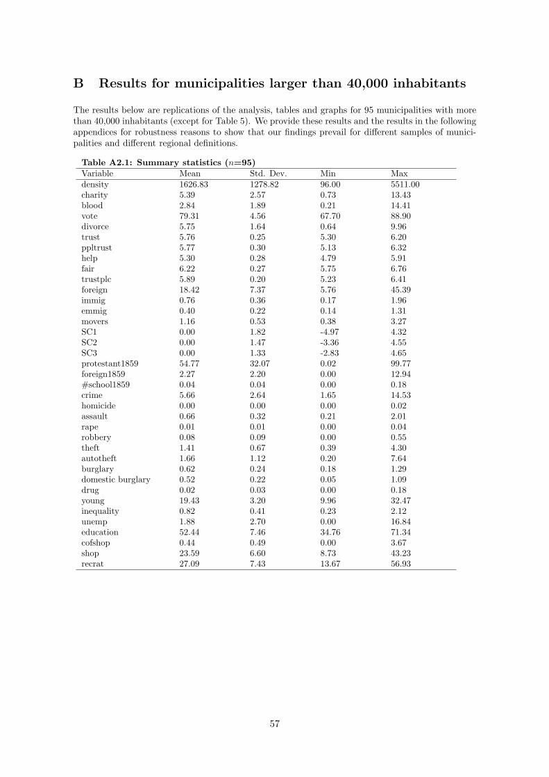
B Results for municipalities larger than 40,000 inhabitants

The results below are replications of the analysis, tables and graphs for 95 municipalities with morethan 40,000 inhabitants (except for Table 5). We provide these results and the results in the followingappendices for robustness reasons to show that our findings prevail for different samples of munici-palities and different regional definitions.

Table A2.1: Summary statistics (n=95)Variable Mean Std. Dev. Min Maxdensity 1626.83 1278.82 96.00 5511.00charity 5.39 2.57 0.73 13.43blood 2.84 1.89 0.21 14.41vote 79.31 4.56 67.70 88.90divorce 5.75 1.64 0.64 9.96trust 5.76 0.25 5.30 6.20ppltrust 5.77 0.30 5.13 6.32help 5.30 0.28 4.79 5.91fair 6.22 0.27 5.75 6.76trustplc 5.89 0.20 5.23 6.41foreign 18.42 7.37 5.76 45.39immig 0.76 0.36 0.17 1.96emmig 0.40 0.22 0.14 1.31movers 1.16 0.53 0.38 3.27SC1 0.00 1.82 -4.97 4.32SC2 0.00 1.47 -3.36 4.55SC3 0.00 1.33 -2.83 4.65protestant1859 54.77 32.07 0.02 99.77foreign1859 2.27 2.20 0.00 12.94#school1859 0.04 0.04 0.00 0.18crime 5.66 2.64 1.65 14.53homicide 0.00 0.00 0.00 0.02assault 0.66 0.32 0.21 2.01rape 0.01 0.01 0.00 0.04robbery 0.08 0.09 0.00 0.55theft 1.41 0.67 0.39 4.30autotheft 1.66 1.12 0.20 7.64burglary 0.62 0.24 0.18 1.29domestic burglary 0.52 0.22 0.05 1.09drug 0.02 0.03 0.00 0.18young 19.43 3.20 9.96 32.47inequality 0.82 0.41 0.23 2.12unemp 1.88 2.70 0.00 16.84education 52.44 7.46 34.76 71.34cofshop 0.44 0.49 0.00 3.67shop 23.59 6.60 8.73 43.23recrat 27.09 7.43 13.67 56.93

57

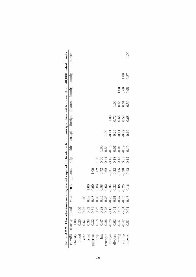
Tab

leA

2.2:

Cor

rela

tion

sam

ong

soci

alca

pit

alin

dic

ator

sfo

rm

unic

ipal

itie

sw

ith

mor

eth

an40

,000

inhab

itan

ts(n

=95

)ch

arity

bloo

dvo

tetr

ust

pplt

rust

help

fair

trus

tplc

fore

ign

divo

rce

imm

igem

mig

mov

ers

char

ity

1.00

bloo

d0.

201.

00vo

te0.

670.

221.

00tr

ust

0.38

0.32

0.48

1.00

pplt

rust

0.32

0.31

0.48

0.90

1.00

help

0.18

0.22

0.33

0.83

0.62

1.00

fair

0.47

0.28

0.44

0.88

0.72

0.60

1.00

trus

tplc

0.26

0.28

0.25

0.62

0.62

0.44

0.54

1.00

fore

ign

-0.7

3-0

.17

-0.7

0-0

.34

-0.3

1-0

.15

-0.1

6-0

.41

1.00

divo

rce

-0.6

2-0

.04

-0.6

1-0

.22

-0.2

2-0

.18

-0.0

7-0

.29

0.72

1.00

imm

ig-0

.47

0.07

-0.3

7-0

.08

-0.0

50.

15-0

.04

-0.1

10.

660.

551.

00em

mig

-0.4

7-0

.04

-0.4

4-0

.25

-0.2

00.

05-0

.19

-0.2

70.

580.

310.

681.

00m

over

s-0

.51

0.04

-0.4

3-0

.16

-0.1

20.

12-0

.10

-0.1

90.

680.

500.

950.

871.

00

58

Tab

leA

2.3:

OLS

resu

lts

for

crim

ean

dal

tern

ativ

ein

dic

ator

sfo

rso

cial

capital

for

munic

ipal

itie

sw

ith

mor

eth

an40

,000

inhab

itan

ts(b

ase)

(1)

(2)

(3)

(4)

(5)

(6)

(7)

(8)

(9)

(10)

(11)

char

ity

bloo

dvo

tetr

ust

trus

tplc

fore

ign

divo

rce

mov

ers

SC1

SC2

SC3

dens

ity

0.17

20.

403

0.34

90.

398

0.40

60.

145

0.28

70.

346

0.18

70.

286

0.25

1(0

.075

)**

(0.0

69)*

**(0

.067

)***

(0.0

70)*

**(0

.071

)***

(0.0

76)*

(0.0

80)*

**(0

.064

)***

(0.0

75)*

*(0

.070

)***

(0.0

72)*

**ed

ucat

ion

-0.2

00-0

.347

-0.1

85-0

.316

-0.3

40-0

.134

-0.3

08-0

.265

-0.1

36-0

.179

-0.1

60(0

.076

)**

(0.0

82)*

**(0

.079

)**

(0.0

84)*

**(0

.084

)***

(0.0

74)*

(0.0

80)*

**(0

.080

)***

(0.0

80)*

(0.0

81)*

*(0

.078

)**

unem

p-0

.026

0.00

6-0

.022

-0.0

22-0

.013

-0.0

02-0

.011

0.03

7-0

.058

-0.0

62-0

.039

(0.0

40)

(0.0

65)

(0.0

44)

(0.0

64)

(0.0

64)

(0.0

40)

(0.0

47)

(0.0

49)

(0.0

44)

(0.0

47)

(0.0

41)

youn

g0.

241

0.27

20.

234

0.22

50.

204

0.24

40.

115

0.15

20.

258

0.31

00.

302

(0.0

76)*

**(0

.107

)**

(0.0

94)*

*(0

.089

)**

(0.0

84)*

*(0

.092

)***

(0.1

18)

(0.0

91)*

(0.1

00)*

*(0

.094

)***

(0.0

95)*

**SC

-0.4

60-0

.175

-0.3

08-0

.343

-0.4

460.

523

0.29

60.

299

-0.2

7-0

.257

-0.3

17(0

.080

)***

(0.0

77)*

*(0

.075

)***

(0.1

82)*

(0.2

69)

(0.0

95)*

**(0

.114

)**

(0.0

90)*

**(0

.050

)***

(0.0

52)*

**(0

.058

)***

cons

tant

0.02

20.

022

0.02

20.

054

0.06

50.

022

0.02

20.

022

0.02

20.

022

0.02

2(0

.060

)(0

.068

)(0

.065

)(0

.071

)(0

.075

)(0

.059

)(0

.065

)(0

.064

)(0

.059

)(0

.062

)(0

.061

)n

9595

9595

9595

9595

9595

95R

-squ

ared

0.66

0.57

0.61

0.56

0.57

0.68

0.60

0.62

0.68

0.64

0.66

Adj

Rsq

r0.

650.

550.

590.

540.

540.

660.

580.

590.

660.

620.

64D

epen

den

tva

riable

isth

eov

erall

crim

era

te.

All

vari

able

sare

standard

ized

.

Robust

standard

erro

rsin

pare

nth

eses

.*

signifi

cant

at

10%

;**

signifi

cant

at

5%

;***

signifi

cant

at

1%

.

59

Tab

leA

2.4:

OLS

resu

lts

for

crim

ean

dal

tern

ativ

ein

dic

ator

sfo

rso

cial

capital

for

munic

ipal

itie

sw

ith

mor

eth

an40

,000

inhab

itan

ts(e

xte

nded

)(1

)(2

)(3

)(4

)(5

)(6

)(7

)(8

)(9

)(1

0)(1

1)ch

arity

bloo

dvo

tetr

ust

trus

tplc

fore

ign

divo

rce

mov

ers

SC1

SC2

SC3

dens

ity

0.11

80.

330.

266

0.31

10.

324

0.11

30.

267

0.31

0.13

10.

201

0.17

9(0

.071

)(0

.066

)***

(0.0

70)*

**(0

.070

)***

(0.0

70)*

**(0

.073

)(0

.080

)***

(0.0

68)*

**(0

.073

)*(0

.070

)***

(0.0

71)*

*ed

ucat

ion

-0.1

54-0

.256

-0.1

61-0

.227

-0.2

35-0

.126

-0.2

66-0

.235

-0.1

27-0

.137

-0.1

35(0

.064

)**

(0.0

67)*

**(0

.065

)**

(0.0

69)*

**(0

.067

)***

(0.0

66)*

(0.0

68)*

**(0

.067

)***

(0.0

69)*

(0.0

68)*

*(0

.065

)**

unem

p-0

.036

-0.0

16-0

.029

-0.0

48-0

.050

-0.0

14-0

.014

0.01

7-0

.064

-0.0

74-0

.047

(0.0

38)

(0.0

33)

(0.0

40)

(0.0

39)

(0.0

38)

(0.0

46)

(0.0

34)

(0.0

34)

(0.0

50)

(0.0

44)*

(0.0

43)

youn

g0.

124

0.14

30.

133

0.10

10.

066

0.13

90.

023

0.05

90.

155

0.19

30.

19(0

.085

)(0

.112

)(0

.108

)(0

.099

)(0

.088

)(0

.102

)(0

.118

)(0

.101

)(0

.112

)(0

.105

)*(0

.107

)*in

equa

lity

0.03

7-0

.033

0.13

80.

022

-0.0

190.

043

0.01

30.

001

0.09

40.

088

0.09

2(0

.065

)(0

.074

)(0

.074

)*(0

.068

)(0

.068

)(0

.066

)(0

.072

)(0

.073

)(0

.067

)(0

.066

)(0

.068

)sh

op0.

136

0.14

30.

139

0.14

70.

126

0.14

10.

098

0.11

50.

141

0.16

40.

151

(0.0

59)*

*(0

.069

)**

(0.0

61)*

*(0

.068

)**

(0.0

72)*

(0.0

61)*

*(0

.068

)(0

.071

)(0

.055

)**

(0.0

57)*

**(0

.057

)***

recr

at0.

129

0.15

90.

142

0.14

90.

184

0.14

90.

155

0.12

10.

149

0.14

60.

142

(0.0

60)*

*(0

.067

)**

(0.0

62)*

*(0

.065

)**

(0.0

60)*

**(0

.054

)***

(0.0

61)*

*(0

.067

)*(0

.052

)***

(0.0

56)*

*(0

.055

)**

cofs

hop

0.19

70.

197

0.21

00.

237

0.24

30.

106

0.17

30.

164

0.15

00.

203

0.18

4(0

.069

)***

(0.0

77)*

*(0

.079

)***

(0.0

82)*

**(0

.073

)***

-0.0

64(0

.077

)**

(0.0

90)*

(0.0

65)*

*(0

.070

)***

(0.0

68)*

**SC

-0.4

21-0

.190

-0.3

16-0

.420

-0.6

770.

471

0.21

00.

195

-0.2

55-0

.257

-0.3

05(0

.079

)***

(0.0

76)*

*(0

.079

)***

(0.1

71)*

*(0

.272

)**

(0.0

93)*

**(0

.111

)*(0

.081

)**

(0.0

47)*

**(0

.049

)***

(0.0

55)*

**C

onst

ant

0.02

20.

022

0.02

20.

061

0.08

80.

022

0.02

20.

022

0.02

20.

022

0.02

2(0

.054

)(0

.061

)(0

.059

)(0

.064

)(0

.067

)(0

.055

)(0

.061

)(0

.061

)(0

.054

)(0

.055

)(0

.055

)n

9595

9595

9595

9595

9595

95R

-squ

ared

0.74

0.67

0.69

0.66

0.68

0.73

0.67

0.67

0.74

0.73

0.73

Adj

Rsq

r0.

710.

640.

660.

630.

650.

700.

630.

630.

710.

700.

71D

epen

den

tva

riable

isth

eov

erall

crim

era

te.

All

vari

able

sare

standard

ized

Robust

standard

erro

rsin

pare

nth

eses

.*

signifi

cant

at

10%

;**

signifi

cant

at

5%

;***

signifi

cant

at

1%

.

60

Table A2.5: 2SLS results for crime and social capital for municipalities with more than 40,000 inhabitants(1) 1st stage (2) 2SLS (3) 1st stage (4) 2SLS (5) 1st stage (6) 2SLSSC1 crime SC2 crime SC3 crime

density -0.690 0.104 -0.439 0.155 -0.447 0.138(0.146)*** (0.086) (0.125)*** (0.078)** (0.116)*** (0.084)*

education 0.493 -0.108 0.447 -0.093 0.372 -0.099(0.134)*** (0.075) (0.128)*** (0.078) (0.101)*** (0.072)

unemp -0.210 -0.073 -0.260 -0.100 -0.132 -0.060(0.143) (0.057) (0.101)** (0.055)* (0.088) (0.050)

young 0.180 0.168 0.328 0.238 0.244 0.225(0.163) (0.110) (0.117)*** (0.107)** (0.118)** (0.107)**

inequality 0.293 0.108 0.301 0.119 0.276 0.118(0.124)** (0.066) (0.100)*** (0.069)* (0.090)*** (0.066)*

shop 0.057 0.144 0.163 0.177 0.108 0.159(0.120) (0.052)*** (0.105) (0.056)*** (0.090) (0.055)***

recrat 0.166 0.150 0.149 0.146 0.128 0.141(0.139) (0.048)*** (0.109) (0.052)*** (0.090) (0.052)***

cofshop -0.219 0.140 -0.037 0.195 -0.098 0.173(0.146) (0.062)** (0.110) (0.064)*** (0.096) (0.061)***

foreign1859 -0.442 -0.320 -0.250(0.105)*** (0.116)*** (0.085)***

protestant1859 0.263 0.343 0.365(0.114)** (0.105)*** (0.082)***

#school1859 0.432 0.350 0.289(0.109)*** (0.103)*** (0.081)***

SC1 -0.288(0.073)***

SC2 -0.340(0.081)***

SC3 -0.383(0.085)***

Constant 0.000 0.022 0.000 0.022 0.000 0.022(0.109) (0.051) (0.099) (0.053) (0.086) (0.052)

n 95 95 95 95 95 95Adj R sqr 0.66 0.71 0.57 0.69 0.60 0.70R-squared 0.70 0.62 0.65F-test instrm. 17.73 17.55 20.88overid 5.20 (0.07)* 2.44 (0.30) 1.95 (0.38)Dependent variable is the overall crime rate. All variables are standardized. Columns 1, 3 and 5 are the first stage results.

Robust standard errors in parentheses. * significant at 10%; ** significant at 5%; *** significant at 1%.

F-test is a test of joint significance of the instruments.

overid is a test of over identification. Null hypothesis: Over-identifying restrictions are valid.

61

Table A2.6: Different 2SLS specifications for crime and social capitalSC1 SC2 SC3

(1) 1st stage (2) 2SLS (3) 1st stage (4) 2SLS (5) 1st stage (6) 2SLSSC crime SC crime SC crime

foreign1859 -0.547 -0.163 -0.450 -0.198 -0.385 -0.232(0.117)*** (0.086)* (0.119)*** (0.105)* (0.095)*** (0.116)**

F-test instrm. 21.69*** 14.28*** 16.28***protestant1859 0.505 -0.443 0.528 -0.423 0.513 -0.436

(0.116)*** (0.108)*** (0.097)*** (0.105)*** (0.077)*** (0.102)***F-test instrm. 18.96*** 29.15*** 43.58***#school1859 0.526 -0.317 0.465 -0.359 0.407 -0.410

(0.104)*** (0.104)*** (0.098)*** (0.131)*** (0.079)*** (0.148)***F-test instrm. 25.38*** 22.48*** 26.35***Robust standard errors in parentheses. * significant at 10%; ** significant at 5%; *** significant at 1%.

All coefficients are obtained from the 2SLS model (equation 4) when it is estimated by including instruments individually.

rather than as a group of three. F-test stands for the significance of the instrument in the first stage.

Detailed results are available from the authors upon request.

62

Tab

leA

2.7:

Sum

mar

yre

sult

sfo

rcr

ime

cate

gori

esan

din

dic

ator

sof

soci

alca

pital

for

munic

ipal

itie

sw

ith

mor

eth

an40

,000

inhab

itan

tsn=

95ch

arity

bloo

dvo

tetr

ust

trus

tplc

fore

ign

divo

rce

mov

ers

SCSC

1SC

2ex

pec

ted

sign

(-)

(-)

(-)

(-)

(-)

(+)

(+)

(+)

(-)

(-)

(-)

crim

e**

***

***

****

***

***

***

***

***

hom

icid

e**

assa

ult

***

***

***

***

***

***

***

***

***

***

*ra

pe**

****

***

***

***

***

***

**ro

bber

y**

****

****

***

****

***

***

thef

t**

***

***

***

***

***

***

*au

toth

eft

***

***

***

***

***

***

***

*bu

rgla

ry**

**

***

***

dom

esti

cbu

rgla

ry**

***

***

***

***

***

***

drug

***

***

***

***

***

***

***

***

*T

he

signifi

cance

level

sder

ive

from

esti

mati

on

ofth

eex

tended

model

for

each

crim

eca

tegory

and

vary

ing

soci

alca

pit

alin

dic

ato

rs.

See

Table

8.

Robust

standard

erro

rsin

pare

nth

eses

.*

signifi

cant

at

10%

;**

signifi

cant

at

5%

;***

signifi

cant

at

1%

.

63

-3-2-1012Voter turnout

-2-1

01

23

Volu

ntar

y co

ntrib

utio

ns-10123

Blood donations-2

-10

12

3Vo

lunt

ary

cont

ribut

ions

-2-1012Percentage of foreigners

-2-1

01

23

Volu

ntar

y co

ntrib

utio

ns

-3-2-1012Divorce rate

-2-1

01

23

Volu

ntar

y co

ntrib

utio

ns

-10123Blood donations

-3-2

-10

12

Vot

er tu

rnou

t

-2-1012Percentage of foreigners

-3-2

-10

12

Vote

r tur

nout

-3-2-1012Divorce rates

-3-2

-10

12

Vote

r tur

nout

-2-1012Percentage of foreigners

-10

12

3Bl

ood

dona

tions

-3-2-1012Divorce rates

-10

12

3Bl

ood

dona

tions

-2-1012Percentage of foreigners

-3-2

-10

12

Div

orce

rate

s

Fig

ure

7:Sc

atte

rplo

tsof

soci

alca

pita

lin

dica

tors

for

95m

unic

ipal

itie

sw

ith

mor

eth

an40

,000

inha

bita

nts

64

-2-1012overall crime

-2-1

01

23

volu

ntar

y co

ntrib

utio

nsco

ef =

-.46

, (ro

bust

) se

= .0

8, t

= -5

.775

-2-1012overall crime

-20

24

6bl

ood

dona

tions

coef

= -.

175,

(rob

ust)

se =

.077

, t =

-2.2

78

-2-1012overall crime

-2-1

01

2vo

ter t

urno

utco

ef =

-.3

08, (

robu

st) s

e =

.075

, t =

-4.1

17

-2-1012overall crime

-1-.5

0.5

1ge

nera

lized

trus

tco

ef =

-.34

3, (

robu

st) s

e =

.182

, t =

-1.8

82

-2-1012overall crime

-2-1

01

2pe

rcen

tage

of f

orei

gner

sco

ef =

.523

, (ro

bust

) se

= .0

95, t

= 5

.513

-2-1012overall crime

-2-1

01

2di

vorc

e ra

tes

coef

= .2

96, (

robu

st) s

e =

.114

, t =

2.5

89

Not

e: A

dded

-var

iabl

e pl

ots

are

from

OLS

regr

essi

ons

of c

rime

on a

con

stan

t, po

pula

tion

dens

ity, %

of y

oung

, edu

catio

n, u

nem

ploy

men

t and

a s

ocia

l cap

ital i

ndic

ator

.

Fig

ure

8:O

vera

llcr

ime

and

soci

alca

pita

lin

dica

tors

for

95m

unic

ipal

itie

sw

ith

mor

eth

an40

,000

inha

bita

nts

65

-2-1012overall crime

-4-2

02

4so

cial

cap

ital i

ndex

coef

= -.

27, (

robu

st)

se =

.05,

t =

-5.4

08

02468murder

-4-2

02

4so

cial

cap

ital i

ndex

coef

= -.

224,

(ro

bust

) se

= .1

41, t

= -1

.587

-10123assault

-4-2

02

4so

cial

cap

ital in

dex

coef

= -

.384

, (ro

bust

) se

= .0

55, t

= -7

.02

-10123rape

-4-2

02

4so

cial

cap

ital i

ndex

coef

= -.

385,

(ro

bust

) se

= .0

68, t

= -5

.622

-101234robbery

-4-2

02

4so

cial

cap

ital i

ndex

coef

= -

.274

, (ro

bust

) se

= .0

79, t

= -3

.459

-2-10123theft

-4-2

02

4so

cial

cap

ital i

ndex

coef

= -

.214

, (ro

bust

) se

= .0

6, t

= -3

.56

-101234car theft

-4-2

02

4so

cial

cap

ital in

dex

coef

= -

.184

, (ro

bust

) se

= .0

54, t

= -3

.43

-2-10123drug crimes

-4-2

02

4so

cial c

apita

l ind

exco

ef =

-.21

2, (

robu

st) s

e =

.054

, t =

-3.9

3

Not

e: A

dded

-var

iabl

e pl

ots

are

from

OLS

regr

essi

ons

of c

rime

type

s on

a c

onst

ant,

popu

latio

n de

nsity

, % o

f you

ng, e

duca

tion,

une

mpl

oym

ent a

nd s

ocia

l cap

ital i

ndex

.

Fig

ure

9:C

rim

eca

tego

ries

and

soci

alca

pita

lfo

r95

mun

icip

alit

ies

wit

hm

ore

than

40,0

00in

habi

tant

s

66

OLS

*

* O

LS

OLS

* OLS

*

OLS

*

* OLS

2SLS

bet

as

01

23

4

divo

rce

fore

ign

trust

vote

bloo

d

char

ity

OLS

*

OLS

*

OLS

*

OLS

*

* OLS

* O

LS

%10

%5

%1

2SLS

t-ra

tios

12

34

5

divo

rce

fore

ign

trust

vote

bloo

d

char

ity

Fig

ure

10:

Dis

trib

utio

nof

2SLS

coeffi

cien

tsan

dt-

rati

osex

trac

ted

from

the

robu

stne

ssch

eck

67

C Results for municipalities larger than 50,000 inhabitants

The results below are replications in a similar manner for 63 municipalities with more than 50,000inhabitants. Since we have only 63 observations, we did not replicate the results for the extendedmodel and the 2SLS results. The coefficients for different social capital indicators deriving from theextended model are summarized in Table 5.

Table A3.1: Summary statistics (n=63)Variable Mean Std. Dev. Min Maxdensity 1901.88 1373.94 183.00 5511.00charity 4.76 2.49 0.73 13.09blood 3.11 2.19 0.21 14.41vote 78.35 4.32 68.60 88.90divorce 6.08 1.61 1.06 9.96trust 5.76 0.25 5.30 6.20ppltrust 5.76 0.30 5.13 6.32help 5.31 0.28 4.79 5.91fair 6.21 0.27 5.75 6.76trustplc 5.89 0.20 5.23 6.41foreign 20.44 7.14 5.76 45.39immig 0.86 0.37 0.34 1.96emmig 0.44 0.22 0.18 1.31movers 1.30 0.55 0.54 3.27SC1 0.00 1.81 -4.65 4.87SC2 0.00 1.49 -3.19 4.88SC3 0.00 1.37 -2.60 5.09protestant1859 55.42 30.36 1.06 99.77foreign1859 2.43 1.96 0.00 8.64#school1859 0.04 0.04 0.00 0.18crime 6.36 2.82 1.65 14.53homicide 0.00 0.00 0.00 0.01assault 0.75 0.33 0.21 2.01rape 0.01 0.01 0.00 0.04robbery 0.11 0.10 0.01 0.55theft 1.61 0.69 0.39 4.30autotheft 1.88 1.26 0.20 7.64burglary 0.67 0.24 0.22 1.29domestic burglary 0.56 0.23 0.05 1.09drug 0.02 0.04 0.00 0.18young 20.10 3.40 9.96 32.47inequality 0.72 0.36 0.23 1.92unemp 1.86 2.18 0.00 8.53education 53.78 7.32 37.72 71.34cofshop 0.52 0.54 0.00 3.67shop 25.30 5.81 14.94 43.23recrat 26.73 6.65 13.67 41.58

68

Tab

leA

3.2:

Cor

rela

tion

sam

ong

soci

alca

pital

indic

ator

s(n

=63

)ch

arity

bloo

dvo

tetr

ust

pplt

rust

help

fair

trus

tplc

fore

ign

divo

rce

imm

igem

mig

mov

ers

char

ity

1.00

bloo

d0.

321.

00vo

te0.

660.

331.

00tr

ust

0.38

0.30

0.45

1.00

pplt

rust

0.29

0.32

0.40

0.88

1.00

help

0.22

0.15

0.34

0.82

0.56

1.00

fair

0.47

0.28

0.42

0.88

0.70

0.58

1.00

trus

tplc

0.25

0.25

0.21

0.56

0.57

0.41

0.46

1.00

fore

ign

-0.7

4-0

.28

-0.6

3-0

.31

-0.2

2-0

.17

-0.4

2-0

.06

1.00

divo

rce

-0.5

9-0

.12

-0.6

1-0

.15

-0.1

0-0

.05

-0.2

4-0

.11

0.65

1.00

imm

ig-0

.47

-0.0

1-0

.31

-0.0

40.

03-0

.03

-0.1

00.

220.

660.

471.

00em

mig

-0.3

9-0

.05

-0.2

9-0

.20

-0.1

0-0

.17

-0.2

30.

160.

450.

170.

771.

00m

over

s-0

.47

-0.0

3-0

.32

-0.1

1-0

.02

-0.0

9-0

.16

0.20

0.61

0.38

0.97

0.91

1.00

69

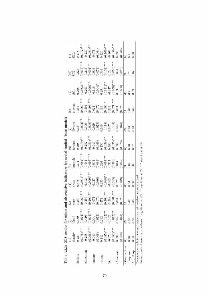
Tab

leA

3.3:

OLS

resu

lts

for

crim

ean

dal

tern

ativ

ein

dic

ator

sfo

rso

cial

capital

(bas

em

odel

)(1

)(2

)(3

)(4

)(5

)(6

)(7

)(8

)(9

)(1

0)(1

1)ch

arity

bloo

dvo

tetr

ust

trus

tplc

fore

ign

divo

rce

mov

ers

SC1

SC2

SC3

dens

ity

0.22

00.

389

0.35

00.

378

0.39

40.

208

0.33

70.

355

0.20

80.

278

0.27

8(0

.076

)***

(0.0

74)*

**(0

.069

)***

(0.0

81)*

**(0

.081

)***

(0.0

79)*

*(0

.092

)***

(0.0

69)*

**(0

.083

)**

(0.0

77)*

**(0

.072

)***

educ

atio

n-0

.288

-0.4

16-0

.256

-0.4

12-0

.434

-0.2

52-0

.396

-0.3

94-0

.201

-0.2

45-0

.239

(0.0

98)*

**(0

.095

)***

(0.1

00)*

*(0

.099

)***

(0.0

97)*

**(0

.093

)***

(0.0

99)*

**(0

.093

)***

(0.0

96)*

*(0

.094

)**

(0.0

94)*

*un

emp

-0.0

400.

004

-0.0

71-0

.027

-0.0

04-0

.049

-0.0

290.

024

-0.1

16-0

.098

-0.0

71(0

.068

)(0

.075

)(0

.070

)(0

.086

)(0

.081

)(0

.066

)(0

.075

)(0

.072

)(0

.064

)*(0

.071

)(0

.064

)yo

ung

0.24

20.

292

0.27

10.

250

0.22

60.

256

0.16

80.

169

0.29

40.

344

0.32

6(0

.085

)***

(0.1

22)*

*(0

.104

)**

(0.0

98)*

*(0

.094

)**

(0.0

98)*

*(0

.118

)(0

.096

)*(0

.111

)**

(0.1

02)*

**(0

.106

)***

SC-0

.373

-0.1

62-0

.288

-0.3

63-0

.363

0.38

60.

167

0.22

3-0

.237

-0.2

4-0

.266

(0.0

82)*

**(0

.077

)**

(0.0

81)*

**(0

.265

)(0

.360

)(0

.095

)***

(0.1

34)

(0.0

71)*

**(0

.050

)***

(0.0

50)*

**(0

.056

)***

Con

stan

t0.

034

0.03

40.

034

0.07

70.

078

0.03

40.

034

0.03

40.

034

0.03

40.

034

(0.0

69)

(0.0

76)

(0.0

73)

(0.0

79)

(0.0

88)

(0.0

70)

(0.0

76)

(0.0

73)

(0.0

68)

(0.0

70)

(0.0

69)

Obs

erva

tion

s63

6363

6363

6363

6363

6363

R-s

quar

ed0.

700.

650.

670.

640.

640.

700.

640.

670.

710.

700.

71A

djR

sqr

0.68

0.62

0.65

0.60

0.60

0.67

0.61

0.64

0.69

0.67

0.68

Dep

enden

tva

riable

isth

eov

erall

crim

era

te.

All

vari

able

sare

standard

ized

.

Robust

standard

erro

rsin

pare

nth

eses

.*

signifi

cant

at

10%

;**

signifi

cant

at

5%

;***

signifi

cant

at

1%

.

70

-3-2-1012Voter turnout

-2-1

01

2Vo

lunt

ary

cont

ribut

ions

-2-10123Blood donations

-2-1

01

2Vo

lunt

ary

cont

ribut

ions

-2-1012Percentage of foreigners

-2-1

01

2Vo

lunt

ary

cont

ribut

ions

-3-2-1012Divorce rate

-2-1

01

2Vo

lunt

ary

cont

ribut

ions

-2-10123Blood donations

-3-2

-10

12

Vot

er tu

rnou

t

-2-1012Percentage of foreigners

-3-2

-10

12

Vote

r tur

nout

-3-2-1012Divorce rates

-3-2

-10

12

Vote

r tur

nout

-2-1012Percentage of foreigners

-2-1

01

23

Bloo

d do

natio

ns

-3-2-1012Divorce rates

-2-1

01

23

Bloo

d do

natio

ns

-2-1012Percentage of foreigners

-3-2

-10

12

Div

orce

rate

s

Fig

ure

11:

Ove

rall

crim

ean

dso

cial

capi

talin

dica

tors

for

63m

unic

ipal

itie

sw

ith

mor

eth

an50

,000

inha

bita

nts

71

-2-1012overall crime

-2-1

01

23

volu

ntar

y co

ntrib

utio

nsco

ef =

-.55

2, (

robu

st) s

e =

.121

, t =

-4.5

74

-2-1012overall crime

-20

24

6bl

ood

dona

tions

coef

= -.

143,

(rob

ust)

se =

.068

, t =

-2.1

12

-2-1012overall crime

-2-1

01

2vo

ter t

urno

utco

ef =

-.3

53, (

robu

st) s

e =

.099

, t =

-3.5

52

-2-1012overall crime

-1-.5

0.5

1ge

nera

lized

trus

tco

ef =

-.3,

(ro

bust

) se

= .2

19, t

= -

1.37

2

-2-1012overall crime

-10

12

perc

enta

ge o

f for

eign

ers

coef

= .4

56, (

robu

st) s

e =

.112

, t =

4.0

67

-2-1012overall crime

-2-1

01

2di

vorc

e ra

tes

coef

= .2

01, (

robu

st) s

e =

.161

, t =

1.2

52

Not

e: A

dded

-var

iabl

e pl

ots

are

from

OLS

regr

essi

ons

of c

rime

on a

con

stan

t, po

pula

tion

dens

ity, %

of y

oung

, edu

catio

n, u

nem

ploy

men

t and

a s

ocia

l cap

ital i

ndic

ator

.

Fig

ure

12:

Ove

rall

crim

ean

dso

cial

capi

talin

dica

tors

for

63m

unic

ipal

itie

sw

ith

mor

eth

an50

,000

inha

bita

nts

72

-2-1012overall crime

-4-2

02

4so

cial

cap

ital i

ndex

coef

= -

.303

, (ro

bust

) se

= .0

67, t

= -4

.551

-1012murder

-4-2

02

4so

cial

cap

ital i

ndex

coef

= -.

216,

(ro

bust

) se

= .0

91, t

= -2

.376

-2-10123assault

-4-2

02

4so

cial

cap

ital i

ndex

coef

= -

.472

, (ro

bust

) se

= .0

84, t

= -5

.609

-2-10123rape

-4-2

02

4so

cial

cap

ital i

ndex

coef

= -.

467,

(ro

bust

) se

= .1

02, t

= -4

.558

-2024robbery

-4-2

02

4so

cial

cap

ital i

ndex

coef

= -

.398

, (ro

bust

) se

= .1

21, t

= -3

.291

-1012theft

-4-2

02

4so

cial c

apita

l ind

exco

ef =

-.19

3, (

robu

st) s

e =

.07,

t =

-2.7

61-2024

car theft-4

-20

24

soci

al c

apita

l ind

exco

ef =

-.1

44, (

robu

st) s

e =

.083

, t =

-1.7

46

-10123drug crimes

-4-2

02

4so

cial

cap

ital i

ndex

coef

= -.

199,

(ro

bust

) se

= .0

72, t

= -2

.773

Not

e: A

dded

-var

iabl

e pl

ots

are

from

OLS

regr

essi

ons

of c

rime

type

s on

a c

onst

ant,

popu

latio

n de

nsity

, % o

f you

ng, e

duca

tion,

une

mpl

oym

ent a

nd s

ocia

l cap

ital i

ndex

.

Fig

ure

13:

Cri

me

cate

gori

esan

dso

cial

capi

talfo

r63

mun

icip

alit

ies

wit

hm

ore

than

50,0

00in

habi

tant

s

73

D Results for 40 NUTS 3 regions

To check whether we obtain similar results for a different regional definition rather than municipalities,we constructed another data set comprising the same indicators for 40 NUTS 3 regions. Detailedinformation on the NUTS definition for the Netherlands is available from the Eurostat webpage[http://ec.europa.eu/eurostat/ramon/nuts/home regions en.html]. The table below summarizes theNUTS 1, NUTS 2 and NUTS 3 definitions. Due to the limited number of observations (n=40) weonly provide summary statistics, correlations of social capital indicators and figures that plot theadded value of social capital on crime. The coefficients for different social capital indicators derivingfrom the extended model are summarized in Table 5.

NUTS1 NUTS2 NUTS3 NUTS 1 region NUTS 2 region NUTS 3 region1 11 111 Noord-Nederland Groningen Oost-Groningen1 11 112 Noord-Nederland Groningen Delfzijl en omgeving1 11 113 Noord-Nederland Groningen Overig Groningen1 12 121 Noord-Nederland Friesland Noord-Friesland1 12 122 Noord-Nederland Friesland Zuidwest-Friesland1 12 123 Noord-Nederland Friesland Zuidoost-Friesland1 13 131 Noord-Nederland Drenthe Noord-Drenthe1 13 132 Noord-Nederland Drenthe Zuidoost-Drenthe1 13 133 Noord-Nederland Drenthe Zuidwest-Drenthe2 21 211 Oost-Nederland Overijssel Noord-Overijssel2 21 212 Oost-Nederland Overijssel Zuidwest-Overijssel2 21 213 Oost-Nederland Overijssel Twente2 22 221 Oost-Nederland Gelderland Veluwe2 22 222 Oost-Nederland Gelderland Achterhoek2 22 223 Oost-Nederland Gelderland Arnhem/Nijmegen2 22 224 Oost-Nederland Gelderland Zuidwest-Gelderland2 23 230 Oost-Nederland Flevoland Flevoland3 31 310 West-Nederland Utrecht Utrecht3 32 321 West-Nederland Noord-Holland Kop van Noord-Holland3 32 322 West-Nederland Noord-Holland Alkmaar en omgeving3 32 323 West-Nederland Noord-Holland IJmond3 32 324 West-Nederland Noord-Holland Agglomeratie Haarlem3 32 325 West-Nederland Noord-Holland Zaanstreek3 32 326 West-Nederland Noord-Holland Groot-Amsterdam3 32 327 West-Nederland Noord-Holland Het Gooi en Vechtstreek3 33 331 West-Nederland Zuid-Holland Agglomeratie Leiden en Bollenstreek3 33 332 West-Nederland Zuid-Holland Agglomeratie ’s-Gravenhage3 33 333 West-Nederland Zuid-Holland Delft en Westland3 33 334 West-Nederland Zuid-Holland Oost-Zuid-Holland3 33 335 West-Nederland Zuid-Holland Groot-Rijnmond3 33 332 West-Nederland Zuid-Holland Agglomeratie ’s-Gravenhage3 33 333 West-Nederland Zuid-Holland Delft en Westland3 33 334 West-Nederland Zuid-Holland Oost-Zuid-Holland3 33 335 West-Nederland Zuid-Holland Groot-Rijnmond3 33 336 West-Nederland Zuid-Holland Zuidoost-Zuid-Holland3 34 341 West-Nederland Zeeland Zeeuwsch-Vlaanderen3 34 342 West-Nederland Zeeland Overig Zeeland4 41 411 Zuid-Nederland Noord-Brabant West-Noord-Brabant4 41 412 Zuid-Nederland Noord-Brabant Midden-Noord-Brabant4 41 413 Zuid-Nederland Noord-Brabant Noordoost-Noord-Brabant4 41 414 Zuid-Nederland Noord-Brabant Zuidoost-Noord-Brabant4 42 421 Zuid-Nederland Limburg Noord-Limburg4 42 422 Zuid-Nederland Limburg Midden-Limburg4 42 423 Zuid-Nederland Limburg Zuid-Limburg

74

Table A4.1: Summary statistics (n=40)Variable Mean Std. Dev. Min Maxdensity 654.73 618.01 146.00 3196.00charity 2.43 0.76 0.98 4.85blood 2.37 1.28 0.89 6.68vote 80.88 3.19 74.35 85.55divorce 5.21 1.14 3.74 8.63trust 5.81 0.24 5.30 6.20ppltrust 5.79 0.31 5.13 6.32help 5.35 0.32 4.79 5.91fair 6.26 0.25 5.75 6.76trustplc 5.88 0.25 5.12 6.41foreign 15.25 6.50 7.45 35.36immig 0.76 0.24 0.42 1.49emmig 0.47 0.19 0.25 0.95movers 1.08 0.56 0.45 3.37SC1 0.00 1.84 -4.77 2.90SC2 0.00 1.51 -3.04 2.69SC3 0.00 1.39 -2.56 2.82protestant1859 61.92 30.19 0.89 99.93foreign1859 1.92 1.90 0.00 8.83#school1859 0.05 0.03 0.01 0.15crime 4.56 1.90 2.35 10.75homicide 0.00 0.00 0.00 0.00assault 0.54 0.22 0.30 1.43rape 0.01 0.01 0.00 0.03robbery 0.06 0.07 0.01 0.34theft 1.13 0.49 0.52 3.14autotheft 1.29 0.67 0.30 3.00burglary 0.50 0.16 0.20 1.04domestic burglary 0.43 0.17 0.20 0.82drug 0.02 0.02 0.00 0.11young 18.85 1.80 15.76 24.38inequality 0.78 0.27 0.34 1.39unemp 1.2 0.90 0.00 3.2education 50.55 5.60 39.09 61.15cofshop 0.36 0.35 0.03 2.33shop 20.02 3.10 12.81 28.91recrat 28.24 5.24 17.22 38.60

75

Tab

leA

4.2:

Cor

rela

tion

sam

ong

soci

alca

pital

indic

ator

s(n

=40

)ch

arity

bloo

dvo

tetr

ust

pplt

rust

help

fair

trus

tplc

fore

ign

divo

rce

imm

igem

mig

mov

ers

char

ity

1.00

bloo

d0.

261.

00vo

te0.

640.

491.

00tr

ust

0.32

0.39

0.45

1.00

pplt

rust

0.20

0.40

0.42

0.84

1.00

help

0.41

0.22

0.36

0.80

0.50

1.00

fair

0.22

0.30

0.31

0.81

0.56

0.47

1.00

trus

tplc

0.28

0.20

0.20

0.49

0.57

0.38

0.38

1.00

fore

ign

-0.6

2-0

.39

-0.6

6-0

.22

-0.0

8-0

.17

-0.2

60.

081.

00di

vorc

e-0

.55

-0.3

2-0

.55

-0.1

9-0

.04

-0.1

0-0

.33

-0.0

10.

861.

00im

mig

-0.4

6-0

.01

-0.3

8-0

.13

-0.0

6-0

.11

-0.1

70.

100.

690.

731.

00em

mig

-0.6

4-0

.29

-0.6

4-0

.24

-0.0

7-0

.26

-0.2

00.

180.

800.

680.

701.

00m

over

s-0

.56

-0.3

0-0

.56

-0.2

3-0

.10

-0.1

1-0

.31

0.12

0.90

0.81

0.77

0.80

1.00

76

-2-1012Voter turnout

-2-1

01

2Vo

lunt

ary

cont

ribut

ions

per

inha

bita

nt

-10123Blood donations per inhabitant

-2-1

01

2Vo

lunt

ary

cont

ribut

ions

per

inha

bita

nt

-2-1012Generalized trust

-2-1

01

2V

olun

tary

con

tribu

tions

per

inha

bita

nt

-2-1012Generalized trust

-2-1

01

2Vo

ter t

urno

ut

-2-1012Generalized trust

-10

12

3Bl

ood

dona

tions

per

inha

bita

nt

-2-1012Voter turnout

-10

12

3B

lood

don

atio

ns p

er in

habi

tant

Fig

ure

14:

Scat

terp

lots

ofso

cial

capi

talin

dica

tors

for

40N

UT

S3re

gion

s

77

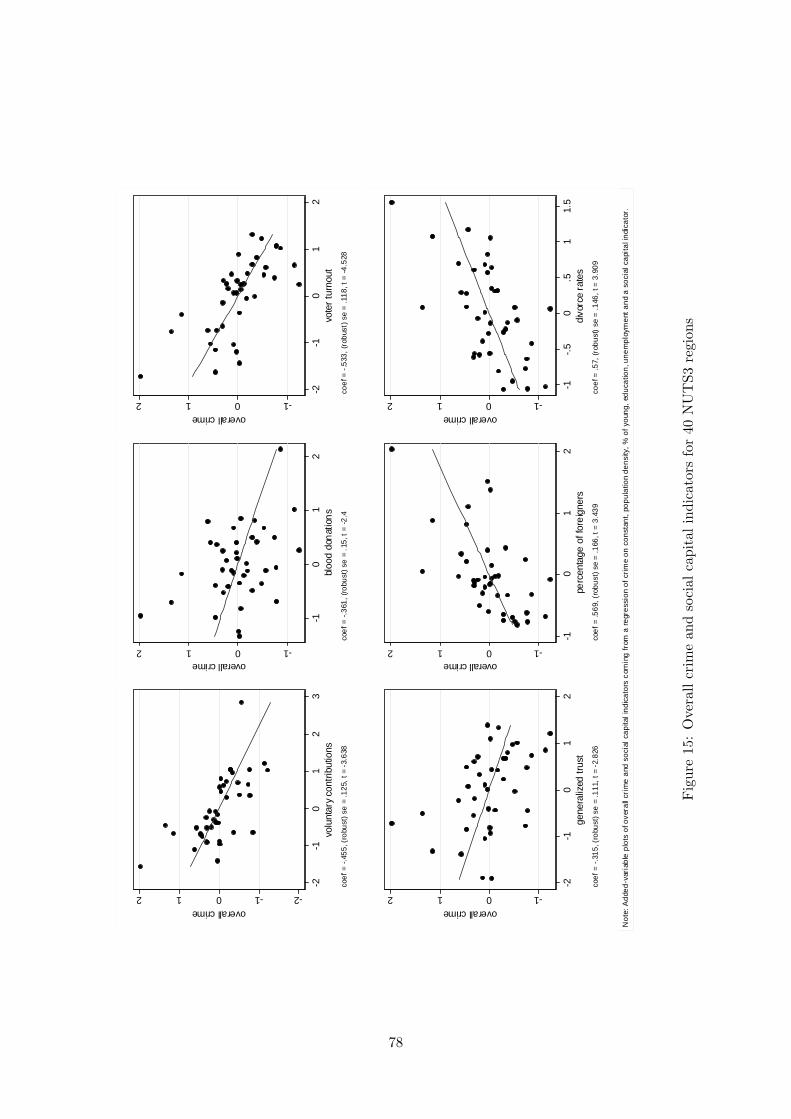
-2-1012overall crime

-2-1

01

23

volu

ntar

y co

ntrib

utio

nsco

ef =

-.45

5, (

robu

st) s

e =

.125

, t =

-3.6

38

-1012overall crime

-10

12

bloo

d do

natio

nsco

ef =

-.36

1, (r

obus

t) se

= .1

5, t

= -2

.4

-1012overall crime

-2-1

01

2vo

ter t

urno

utco

ef =

-.5

33, (

robu

st) s

e =

.118

, t =

-4.5

28

-1012overall crime

-2-1

01

2ge

nera

lized

trus

tco

ef =

-.31

5, (

robu

st) s

e =

.111

, t =

-2.8

26

-1012overall crime

-10

12

perc

enta

ge o

f for

eign

ers

coef

= .5

69, (

robu

st) s

e =

.166

, t =

3.4

39

-1012overall crime

-1-.5

0.5

11.

5di

vorc

e ra

tes

coef

= .5

7, (r

obus

t) se

= .1

46, t

= 3

.909

Not

e: A

dded

-var

iabl

e pl

ots

of o

vera

ll cr

ime

and

soci

al c

apita

l ind

icat

ors

com

ing

from

a re

gres

sion

of c

rime

on c

onst

ant,

popu

latio

n de

nsity

, % o

f you

ng, e

duca

tion,

une

mpl

oym

ent a

nd a

soc

ial c

apita

l ind

icat

or.

Fig

ure

15:

Ove

rall

crim

ean

dso

cial

capi

talin

dica

tors

for

40N

UT

S3re

gion

s

78

-1012overall crime

-4-2

02

soci

al c

apita

l ind

exco

ef =

-.3

76, (

robu

st)

se =

.072

, t =

-5.2

63

-2-10123murder

-4-2

02

soci

al c

apita

l ind

exco

ef =

-.2

64, (

robu

st) s

e =

.106

, t =

-2.5

-2024assault

-4-2

02

soci

al c

apita

l inde

xco

ef =

-.5

07, (

robu

st) s

e =

.12,

t =

-4.2

23

-10123rape

-4-2

02

soci

al c

apita

l ind

exco

ef =

-.51

6, (

robu

st) s

e =

.114

, t =

-4.5

16

-10123robbery

-4-2

02

soci

al c

apita

l ind

exco

ef =

-.4

35, (

robu

st)

se =

.091

, t =

-4.7

67

-10123theft

-4-2

02

socia

l cap

ital i

ndex

coef

= -.

36, (

robu

st)

se =

.101

, t =

-3.5

47-1012

car theft-4

-20

2so

cial

cap

ital i

ndex

coef

= -

.234

, (ro

bust

) se

= .0

72, t

= -3

.235

-2024drug crimes

-4-2

02

soci

al c

apita

l ind

exco

ef =

-.36

7, (

robu

st) s

e =

.204

, t =

-1.7

95

Not

e: A

dded

-var

iabl

e pl

ots

of ty

pes

of c

rime

and

soci

al c

apita

l com

ing

from

a re

gres

sion

of c

rime

type

s on

con

stan

t, po

pula

tion

dens

ity, %

of y

oung

, edu

catio

n, u

nem

ploy

men

t and

soc

ial c

apita

l ind

ex.

Fig

ure

16:

Cri

me

cate

gori

esan

dso

cial

capi

talfo

r40

NU

TS3

regi

ons

79

E Results for 22 large agglomerations

Finally, we also performed analysis at the city level. In the Netherlands there are 22 large agglom-erations as stated by the CBS. These are Groningen (GRN), Leeuwarden (LEUW), Zwolle (ZWL),Enschede (ENS), Apeldoorn (APD), Arnhem (ARN), Nijmegen (NIJM), Amersfoort (AMERSF),Utrecht (UTR), Amsterdam (AMST), Haarlem (HRLM), Leiden (LEID), ’s-Gravenhage (DHG),Rotterdam (ROTD), Dordrecht (DRDR), Breda (BRD), Tilburg (TLB), ’s-Hertogenbosch (SHRT),Eindhoven (EIND), Geleen/Sittard (SITT), Heerlen (HERL) and Maastricht (MAST). We providethe summary statistics, correlation table between social capital indicators, and added-variable plots.Since we have only 22 observations we can not provide detailed analysis and the added-variable plotsare based on OLS regressions of crime on a constant, population density and social capital.

Table A5.1: Summary statistics (n=22)Variable Mean Std. Dev. Min Maxdensity 2311.56 1498.66 455.00 5511.00charity 3.59 2.54 0.73 12.98blood 3.82 3.30 0.54 14.41vote 76.04 4.18 68.60 82.90divorce 6.76 1.73 1.62 9.96trust 5.75 0.25 5.30 6.15ppltrust 5.80 0.31 5.23 6.32help 5.24 0.26 4.81 5.66fair 6.20 0.26 5.75 6.56trustplc 5.94 0.20 5.57 6.41foreign 24.08 8.64 13.71 45.39immig 1.07 0.38 0.51 1.82emmig 0.56 0.23 0.24 1.26movers 1.62 0.54 0.75 2.74SC1 -1.79 1.81 -5.27 2.25SC2 -0.99 1.63 -3.50 3.70SC3 -1.13 1.40 -2.98 3.30protestant1859 47.01 31.45 1.06 86.81foreign1859 2.95 1.82 0.85 8.37#school1859 0.03 0.02 0.00 0.08crime 8.81 2.96 4.02 14.53homicide 0.00 0.00 0.00 0.01assault 0.99 0.40 0.34 2.01rape 0.02 0.01 0.01 0.04robbery 0.18 0.14 0.05 0.55theft 2.23 0.72 1.20 4.30autotheft 2.96 1.39 1.10 7.64burglary 0.81 0.22 0.52 1.29domestic burglary 0.72 0.25 0.05 1.09drug 0.05 0.05 0.01 0.18young 22.03 4.29 10.47 32.47inequality 0.52 0.23 0.23 1.11unemp 2.45 2.35 0.00 7.93education 57.05 6.36 44.27 70.21cofshop 0.94 0.68 0.32 3.67shop 27.88 5.61 17.73 39.76recrat 30.91 6.53 19.37 41.58

80

Tab

leA

5.2:

Cor

rela

tion

sam

ong

soci

alca

pital

indic

ator

sch

arity

bloo

dvo

tetr

ust

pplt

rust

help

fair

trus

tplc

fore

ign

divo

rce

imm

igem

mig

mov

ers

char

ity

1.00

bloo

d0.

651.

00vo

te0.

540.

721.

00tr

ust

0.20

0.49

0.68

1.00

pplt

rust

0.21

0.55

0.68

0.94

1.00

help

-0.0

40.

190.

460.

840.

651.

00fa

ir0.

340.

540.

700.

930.

880.

651.

00tr

ustp

lc0.

350.

220.

340.

600.

510.

580.

541.

00fo

reig

n-0

.62

-0.5

1-0

.65

-0.3

0-0

.32

-0.0

3-0

.45

-0.2

01.

00di

vorc

e-0

.49

-0.3

1-0

.45

-0.0

5-0

.04

0.15

-0.2

2-0

.10

0.67

1.00

imm

ig-0

.57

-0.2

4-0

.41

-0.0

5-0

.08

0.24

-0.2

80.

080.

740.

651.

00em

mig

-0.3

1-0

.25

-0.4

4-0

.46

-0.4

3-0

.30

-0.5

00.

010.

270.

040.

581.

00m

over

s-0

.53

-0.2

7-0

.47

-0.2

3-0

.23

0.04

-0.4

00.

060.

630.

470.

940.

821.

00

81

GR

NLE

UW

ENS

ZWL

APD

ARN

NIJ

M

AMER

SF

UTR

AMST

HR

LM

DR

DR

DH

G

LEID

RO

TD

BRD E

IND

SHR

T

TILB

HE

RL

MAS

TSITT

-3-2-101Voter turnout

-2-1

01

2Vo

lunt

ary

cont

ribut

ions

GR

N

LEU

WEN

S

ZWL

APD

ARN

NIJ

MA

ME

RSF

UTR

AM

ST

HR

LMD

RD

RD

HG

LEID

RO

TDB

RDEI

ND

SH

RT

TILB

HER

L

MAS

T SIT

T

-202468Blood donations

-2-1

01

2Vo

lunt

ary

cont

ribut

ions

GR

NLE

UW

ENS

ZWL

APD

AR

NN

IJM

AMER

SF

UTR

AMS

TH

RLM

DR

DR

DH

G

LEID

RO

TD

BRDEI

ND

SH

RT

TILB

HE

RL

MA

STSIT

T

-1-.50.51Generalized trust

-2-1

01

2V

olun

tary

con

tribu

tions

GR

NLE

UW

ENS

ZWL

APD

AR

NNIJ

M

AME

RSF

UTR

AM

STH

RLM

DR

DR

DH

G

LEID

RO

TD

BRD

EIN

DSH

RT

TILB

HE

RLM

ASTS

ITT

-1-.50.51Generalized trust

-3-2

-10

1Vo

ter t

urno

ut

GR

NLE

UW

ENS

ZWL

APD

ARN

NIJ

M

AME

RSF

UTR

AMSTH

RLM

DR

DR

DH

G

LEID

RO

TD

BRD

EIN

DSH

RT

TILB

HER

LM

AST

SITT

-1-.50.51Generalized trust

-20

24

68

Bloo

d do

natio

ns

GR

N

LEU

WE

NS

ZWL

APD

ARNN

IJM

AME

RSF

UTR

AMST

HR

LMD

RD

RD

HG

LEID

RO

TDB

RD

EIN

D SH

RT

TILB

HER

LMAS

T SIT

T

-202468Blood donations

-3-2

-10

1V

oter

turn

out

Fig

ure

17:

Scat

terp

lots

ofso

cial

capi

talin

dica

tors

for

22la

rges

tag

glom

erat

ions

82

BRD

RO

TD

ARN

APDUTR

GR

N

AM

ST

DR

DR

DH

G

HER

L

NIJ

MTI

LB

SH

RT

MA

ST

ENSSIT

T AM

ER

SF

EIN

D

LEU

W

LEID

HR

LM

ZW

L

-2-1012overall crime

-10

12

3vo

lunt

ary

cont

ribut

ions

coef

= -.

875,

(ro

bust

) se

= .3

07, t

= -2

.849

BR

D

AM

ST

HE

RL

AR

N

RO

TD

DR

DR

SIT

TTI

LB

SH

RT

DH

G

EIN

D

MAS

TA

PD HR

LMAM

ER

SF

EN

S

UT

R NIJ

MLE

UW

LEID

GR

N

ZWL

-2-1012overall crime

-20

24

6bl

ood

dona

tions

coef

= -.

175,

(rob

ust)

se =

.121

, t =

-1.4

48

HE

RL TILBRO

TD M

AST

DH

GAMST

BR

D

SIT

T

AR

N

DR

DR

EIN

D

EN

SSH

RT NIJ

M

UT

R

APD LE

UW

HR

LMGR

N

LEID

ZWL

AM

ER

SF

-2-1012overall crime

-2-1

01

2vo

ter t

urno

utco

ef =

-.4

96, (

robu

st) s

e =

.245

, t =

-2.0

25

RO

TD

MA

STH

ER

L

SIT

T

BR

D

ENS

DH

G DR

DR

TILB

AMS

T

EIN

D

HR

LMSH

RT

UT

R

AM

ER

SF

GR

N LEU

W

AP

D

ZWLN

IJM

ARN LE

ID

-2-1012overall crime

-1-.5

0.5

1ge

nera

lized

trus

tco

ef =

-.62

3, (

robu

st) s

e =

.401

, t =

-1.5

56

HR

LMLEID

GR

N LEU

W

MA

ST

SH

RT

NIJ

M

ZWL

AM

ERS

F

TILBEIN

D SIT

TA

PD

HER

L

DR

DR

UTR B

RD

ARN

EN

SDH

G

RO

TDA

MS

T

-2-1012overall crime

-2-1

01

2pe

rcen

tage

of f

orei

gner

sco

ef =

.625

, (ro

bust

) se

= .1

97, t

= 3

.179

SIT

T

LEID

UTR AM

ER

SF

NIJ

M

HR

LM

TIL

B

ZWL

GR

N

ENS

SH

RT

MA

ST

EIN

D

DR

DR

AP

D

AR

N

LEU

W

BR

D DH

G

HE

RL

RO

TDA

MS

T

-2-1012overall crime

-3-2

-10

1di

vorc

e ra

tes

coef

= .4

71, (

robu

st) s

e =

.272

, t =

1.7

32

Not

e: A

dded

-var

iabl

e pl

ots

of o

vera

ll cr

ime

and

soci

al c

apita

l ind

icat

ors

com

ing

from

a re

gres

sion

of c

rime

on c

onst

ant,

popu

latio

n de

nsity

and

a s

ocia

l cap

ital i

ndic

ator

.

Fig

ure

18:

Ove

rall

crim

ean

dso

cial

capi

talin

dica

tors

for

22la

rges

tag

glom

erat

ions

83

RO

TD

AM

ST

HER

L

DH

G

BR

DAR

N

DR

DR

TILB

MA

ST

EN

S

APDEIN

D

UTR SH

RT

SIT

TLE

UW

NIJ

M AM

ER

SF

GR

N

HR

LMLE

IDZWL

-2-1012overall crime

-4-2

02

4so

cial

cap

ital i

ndex

coef

= -

.406

, (ro

bust

) se

= .0

98, t

= -4

.128

RO

TD AM

ST

HE

RL

DH

GB

RD AR

N

DR

DR

TIL

B

MAS

T

EN

S

AP

D

EIN

DU

TR

SHR

T

SIT

TLE

UW

NIJ

MAM

ER

SFG

RN

HR

LM LEIDZW

L

-1012murder

-4-2

02

4so

cial

cap

ital i

ndex

coef

= -.

302,

(ro

bust

) se

= .0

91, t

= -3

.303

RO

TD

AM

ST

HE

RL

DH

G

BR

DARN

DR

DR

TIL

B

MA

ST

ENS

AP

DE

IND

UTR SH

RT

SIT

T

LEU

W

NIJ

M AM

ER

SF

GR

N

HR

LMLEID ZW

L

-2-10123assault

-4-2

02

4so

cial

cap

ital in

dex

coef

= -

.589

, (ro

bust

) se

= .1

25, t

= -4

.72

RO

TD AM

ST

HE

RL

DH

G

BR

DAR

ND

RD

RT

ILB

MAS

T

ENS

AP

D

EIN

D

UTR SH

RT

SIT

T

LEU

W

NIJ

MAM

ER

SFG

RN

HR

LMLEIDZW

L

-2-10123rape

-4-2

02

4so

cial

cap

ital i

ndex

coef

= -.

522,

(ro

bust

) se

= .1

54, t

= -3

.382

RO

TD

AM

ST

HER

L

DH

G

BR

D AR

N

DR

DR

TILB

MA

ST

EN

S

APD EIN

D

UTR SH

RT

SIT

TLE

UW

NIJ

MAM

ER

SF

GR

N

HR

LMLEIDZW

L

-4-2024robbery

-4-2

02

4so

cial

cap

ital i

ndex

coef

= -

.663

, (ro

bust

) se

= .2

14, t

= -3

.101

RO

TDAM

ST

HE

RL

DH

G

BR

DAR

N

DR

DR

TIL

BM

AST

EN

S

AP

D

EIN

D

UT

RSH

RT

SIT

TLE

UW

NIJ

MAM

ER

SF

GR

N

HR

LM LEI

D

ZWL

-10123theft

-4-2

02

4so

cial

cap

ital i

ndex

coef

= -.

324,

(ro

bust

) se

= .1

03, t

= -3

.161

RO

TD AM

ST

HE

RL

DH

G

BRDAR

N

DR

DR

TILB

MA

ST

EN

SA

PDEIN

D

UTR SH

RT

SIT

T

LEU

W

NIJ

M AMER

SFG

RN

HR

LM LEIDZW

L

-2024car theft

-4-2

02

4so

cial

cap

ital i

ndex

coef

= -.

355,

(rob

ust)

se

= .0

99, t

= -3

.6

RO

TDAM

ST

HE

RL

DH

G

BRDA

RN

DR

DR

TILB

MA

ST

EN

S

AP

D

EIN

D

UT

R

SH

RT

SIT

T

LEU

W

NIJ

M AM

ERS

FG

RN

HR

LM LEIDZW

L

-2-10123drug crimes

-4-2

02

4so

cial c

apita

l ind

exco

ef =

-.37

5, (

robu

st) s

e =

.08,

t =

-4.7

02

Not

e: A

dded

-var

iabl

e pl

ots

of ty

pes

of c

rime

and

soci

al c

apita

l com

ing

from

a re

gres

sion

of c

rime

type

s on

con

stan

t, po

pula

tion

dens

ity a

nd s

ocia

l cap

ital i

ndex

.

Fig

ure

19:

Cri

me

cate

gori

esan

dso

cial

capi

talfo

r22

larg

est

aggl

omer

atio

ns

84