the impact of the fracking boom on arab oil producerslkilian/erf_egypt.pdf · 0 the impact of the...
TRANSCRIPT
0
The Impact of the Fracking Boom on Arab Oil Producers
July 30, 2016
Lutz Kilian
University of Michigan CEPR
Abstract: This paper makes four contributions. First, it investigates the extent to which the U.S. fracking boom has caused Arab oil exports to decline since late 2008. Second, the paper quantifies for the first time by how much the U.S. fracking boom has lowered the global price of oil. Using a novel econometric methodology, it is shown that in mid-2014, for example, the Brent price of crude oil was lower by $10 than it would have been in the absence of the fracking boom. Third, the paper provides evidence that the decline in Saudi net foreign assets between mid-2014 and August 2015 would have been reduced by 27 percent in the absence of the fracking boom. Finally, the paper discusses the policy choices faced by Saudi Arabia and other Arab oil producers. JEL Code: Q43, Q33, F14 Key Words: Arab oil producers; Saudi Arabia; shale oil; tight oil; oil price; oil imports; oil exports; refined product exports; oil revenue; foreign exchange reserves; oil supply shock. Acknowledgements: I thank Christiane Baumeister, Bassam Fattouh, and Ryan Kellogg for helpful comments and discussion. This work has benefited from a financial grant from the Economic Research Forum and from comments from two anonymous referees provided by the Forum. The contents and recommendations do not necessarily reflect the views of the Economic Research Forum. Correspondence to: Lutz Kilian, Department of Economics, 611 Tappan Street, Ann Arbor, MI 48109-1220, USA. Email: [email protected].

1
1. Introduction
The use of hydraulic fracturing (or fracking) in conjunction with horizontal drilling and micro-seismic
imaging has made it possible to extract crude oil from rock formations characterized by low permeability.
Oil extracted by these techniques is commonly referred to as tight oil or shale oil to differentiate it from
crude oil extracted by conventional drilling techniques. To date commercial shale oil production has been
largely limited to the United States. The U.S. oil fracking boom is an example of a technological change
in a single industry in one country affecting international trade worldwide. Increased U.S. shale oil
production over time has displaced crude oil exports from Arab oil producing countries, both because the
United States no longer relies as heavily on crude oil imports from Arab countries and because U.S.
refineries have increasingly exported refined products such as gasoline or diesel made from domestically
produced crude oil, causing other countries to cut back on their crude oil imports as well (see Kilian
2016). Whereas the gains to the U.S. economy of the fracking boom are well understood at this point,
little is known to date about the losses this development has imposed on foreign oil producers.
Understanding the implications of the U.S. fracking boom is important not only for policymakers in Arab
economies deciding on how best to respond to the tight oil boom, but it also provides a prime example of
a well-identified exogenous shock to the terms of trade of primary commodity exporters.
This paper quantifies the impact of the U.S. tight oil boom on global oil production, on U.S.
imports of crude oil and exports of refined products as well as Arab exports of crude oil.1 On the basis of
these estimates, I construct an estimate of how the price of oil in global markets would have evolved in
the absence of this boom. Based on a widely used structural econometric model of the global market for
crude oil I show that the cumulative effect of the tight oil boom on the Brent price had been building
gradually, reaching a peak in mid-2014, before declining in late 2014. Whereas in mid-2014 the Brent
price was lower by $10 than it would have been in the absence of the fracking boom, by mid-2015 this
price differential had fallen to $5. My analysis also demonstrates that a very similar price decline would
1 An excellent nontechnical study of the impact of the tight oil boom on Arab oil producers is Fattouh (2014).

2
have occurred between July 2014 and January 2015 even in the absence of increased U.S. shale oil
production, suggesting that increased shale oil production was not the main cause of this price decline.
I use the difference between the actual and the counterfactual global price of crude oil to quantify
the losses in Saudi oil revenue (and hence in Saudi national income) since late 2008 under the maintained
assumption that Saudi oil production remained unchanged by the fracking boom. My analysis shows that
the cumulative losses in Saudi oil revenue caused by fracking by August 2015 had reached 102 billion
dollars. I relate this estimate to the substantial decline in Saudi net foreign assets between mid-2014 and
August 2015. I show that the shale oil boom accounts for 27 percent (or 24 billion U.S. dollars) of this
decline , with the remaining 66 billion dollars reflecting increased oil production by other oil producers,
shifts in oil price expectations, and the weakening of the global economy. I make the case that this decline
is unsustainable and discuss implications of my analysis for Saudi economic policies in the years to come.
The remainder of the paper is organized as follows. In section 2, I review the evolution of crude
oil production in the United States and elsewhere, highlighting the contribution of the U.S. fracking boom
to global oil production growth. Sections 3 and 4 quantify the extent to which the shale oil boom has
reduced Arab oil exports since late 2008, distinguishing between the reduction in U.S. crude oil imports
from Arab oil producers and the reduction in Arab oil exports to the rest of the world caused by increased
U.S. exports of refined products, as U.S. refiners took advantage of access to low-cost domestically
produced crude oil. In section 5, I study the financial implications of the U.S. fracking boom for Arab oil
producers, focusing on Saudi Arabia as the leading example. Building on the analysis in sections 2, 3 and
4, I develop and compare two data-based counterfactuals aimed at estimating the implications of the shale
oil boom for the global price of oil and for Saudi Arabia’s oil revenues between December 2008 and
August 2015. Section 6 relates my preferred estimate of these effects to the dramatic decline in Saudi net
foreign assets since June 2014 and discusses the policy implications for Saudi Arabia in particular.
2. Recent Changes in Oil Production in the United States and Elsewhere
Only a few years ago, a common view among pundits was that world oil production would no longer be
3
able to keep up with growing oil consumption needs. An extreme version of this skepticism was
embodied in the peak oil hypothesis which asserted that global oil production had permanently peaked by
2007 or that the peak was imminent.2 Although economists tend to be skeptical of the peak oil hypothesis
for reasons discussed in Holland (2008, 2013), it was readily apparent at the time that many traditional oil
fields were in decline and that the prospects for discovering more crude oil in regions not ridden with civil
strife were diminishing. Thus, even granting that high oil prices driven by strong demand for oil tend to
provide strong incentives for expanding future oil production, as of 2007, nothing in past experience
guaranteed that this supply response to rising oil prices would be adequate or that it would occur in a
timely manner.
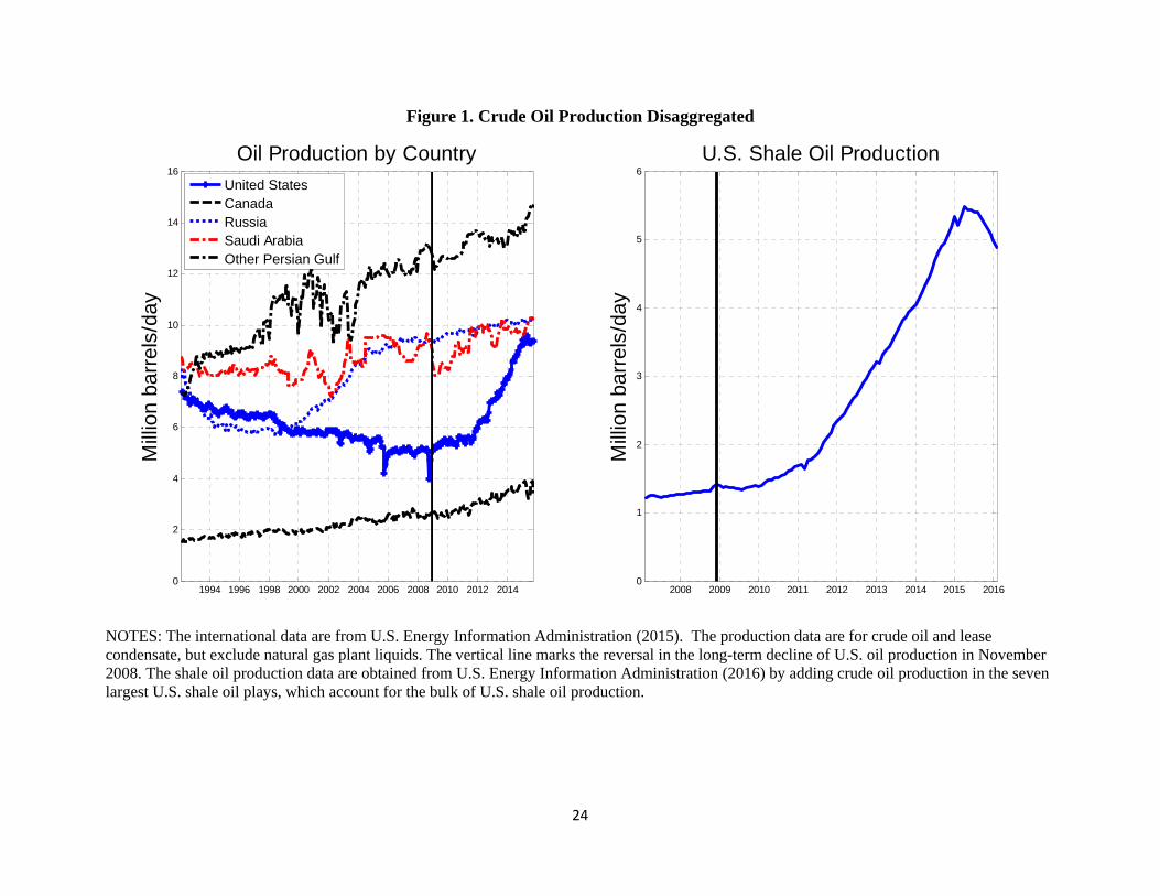
As the left panel of Figure 1 shows, with the benefit of hindsight, these concerns were
unwarranted. Not only did the U.S. fracking boom reverse the long-standing decline in U.S. crude oil
production, but Canadian production of unconventional crude oil from oil sands soared and Russian oil
production reached unprecedented levels. At the same time, both Saudi Arabian and other Persian-Gulf
production growth, which seemed to have levelled off after 2005, accelerated again. This surge in oil
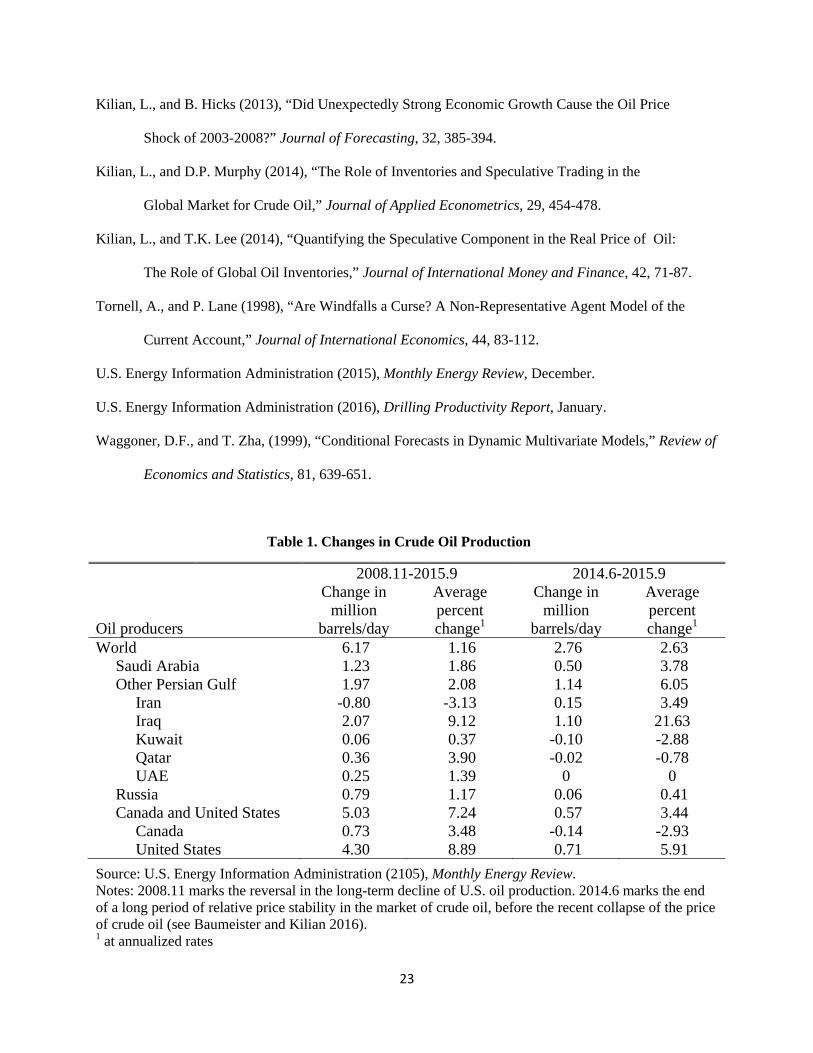
production was more than enough to offset the decline in crude oil production in other countries. Table 1
shows an increase in global oil production of 6.17 million barrels per day (mbd) between November 2008
and September 2015, corresponding to an average rate of increase of 1.16 percent. Average growth
accelerated to 2.63 percent between June 2014 and September 2015. Table 1 dispels the notion that
fracking in the United States alone has been responsible for this surge. Although the United States was
responsible for the bulk of the oil production increase, accounting for an extra 4.3 mbd over the last seven
years, there also have been notable production increases in Iraq (2.07 mbd), Saudi Arabia (1.23 mbd),
Russia (0.79 mbd) and Canada (0.73 mbd) that were unrelated to the fracking boom.
The evolution of U.S. oil production in particular is remarkable, given the long-standing decline
in U.S. oil production that began in the early 1970s and was only briefly reversed by the development of
2 For example, an IMF study by Benes et al. (2015), using data up to 2009, predicted a near doubling of the price of oil over the coming decade based on the view that geological constraints would win out over technological improvements in conserving oil use and in oil extraction.

4
the Alaskan oil fields in the late 1970s. The vertical line in the left panel of Figure 1 refers to the date of
November 2008, which marks the reversal of this trend. It can be shown that this reversal is largely due to
the U.S. fracking boom. The right panel of Figure 1 plots the sum of crude oil production at the Bakken,
Eagle Ford, Haynesville, Marcellus, Niobrara, Permian, and Uttica shale oil plays. These seven regions
account for 92% of U.S. domestic shale oil production growth. Between November 2008 and September
2015, U.S. shale oil production increased by approximately 3.82 / 0.92 4.15 million barrels/day (mbd),
which roughly matches the entry of 4.30 mbd for the change in total U.S. crude oil production in the first
column of Table 1. Thus, throughout this paper, I will treat November 2008 as the beginning of the
fracking boom.
3. Quantifying the Decline in U.S. Crude Oil Imports from Arab Producers
The U.S. oil sector is governed by the following identity, which describes the composition of the total
quantity of crude oil used by the economy: ,t t t t tQ M X C I where tQ is domestic crude oil
production, tM is U.S. crude oil imports, tX is U.S. crude oil exports, tC is the consumption of
crude oil, which refers to crude oil used by U.S. refineries to produce refined products such as
gasoline or diesel for domestic consumption or for export, and tI denotes the change in crude
oil inventories.
The left panel of Figure 2 illustrates how U.S. domestic oil production, crude oil imports and
exports of crude oil have evolved since the 1970s. Three facts stand out. First, as already noted, following
a secular decline in U.S. oil production, U.S. oil production sharply accelerated in late 2008, reflecting the
fracking boom. Second, historically crude oil imports have been rising during economic expansions and
falling during economic downturns. This pattern changed in 2005, even before the fracking boom, when
the U.S. economy learned to make do with less crude oil during an economic expansion amidst high and
rising oil prices. The decline in crude oil imports accelerated during the fracking boom, when increased
domestic shale oil production lowered the U.S. price of oil compared with the global price of oil, reducing

5
U.S. demand for high-cost crude oil imports. The reason for the comparatively low price of shale oil was
a glut of light sweet crude oil in the central United States that reflected transportation bottlenecks within
the United States as well as a ban on U.S. crude oil exports (see Kilian 2016). There have been some
exemptions from this ban, notably for oil exports to Canada, for example, but overall this restriction has
been binding. As a result, U.S. crude oil exports have remained negligible throughout most of this sample.
Only in 2014 and 2015 U.S. oil exports increased somewhat, as the Obama administration allowed for
more flexibility in the interpretation of the law governing U.S. oil exports. As of December 2015,
Congress passed a law lifting the oil export ban, but that policy shift is not yet reflected in the data in
Figure 2.
The right panel of Figure 2 quantifies the total use of crude oil by the U.S. economy, computed as
.t t tQ M X In quantifying the importance of oil imports for the U.S. economy, it is useful to express
U.S. crude oil imports as a share of the amount of crude oil used by the U.S. economy.3 The left panel of
Figure 3 shows the evolution of the share of U.S. crude oil imports from the rest of the world as well as
the share of U.S. crude oil imports from OPEC, from Arab OPEC (defined as Algeria, Iraq, Kuwait, and
Saudi Arabia for our purposes), and from West Africa (Nigeria, Angola).4 The overall import share
declined from a peak of almost 70 percent in the mid-2000s to about 45% in 2015. This pattern is also
found for OPEC oil imports and its components. By 2015 crude oil imports from West Africa fell to near
zero. West African crudes are in direct competition with domestically produced light sweet crude oil in
the United States. As U.S. refiners along the East Coast found ways of substituting shale oil (or lower
priced conventional light sweet crude oil from domestic sources) for these imports, West African crudes
3 This approach controls for fluctuations in the size of the U.S. economy and for slow-moving changes in the energy efficiency of the U.S. economy. During a recession, for example, all else equal, both the use of crude oil by the economy and its oil imports would be expected to fall without affecting the oil import share. In contrast, if the fracking boom displaces crude oil imports from Arab oil producers, this should be reflected in a reduction in the share of U.S. imports from Arab countries in the oil used by the U.S. economy. 4 I approximate crude oil imports from these countries by petroleum imports under the assumption that U.S. product imports from Arab countries are zero. This assumption can be verified for selected dates using data in the EIA’s database for U.S. crude oil imports at the company level. Figure 3 excludes Libya from the Arab oil producers because Libyan oil exports in recent years are driven primarily by political events in Libya. The UAE and Qatar are excluded, because the EIA does not provide monthly data for U.S. imports from these countries, given their small size.

6
were almost entirely displaced. Crude oil imports from Arab OPEC as well fell from about 20 percent of
U.S. oil use as recently as 2008 to under 10 percent in 2015. The reason presumably was that these crudes
no longer could compete with the low price of domestically produced U.S. crude oil and U.S. imports of
heavy Canadian crudes (see Kilian 2016).
The right panel of Figure 3 traces the import shares of four Arab oil producers before and after
November 2008, which marks the beginning of the fracking boom (see Figure 1). We are interested in
whether there are important changes in the dependency of the U.S. economy on oil imports from these
countries. Figure 3 shows a striking drop in the share of U.S. oil imports from Saudi Arabia after
November 2008. After some fluctuations, the Saudi share reaches near 5% in 2015, compared with about
10% initially. Figure 3 also a steady decline in the share of U.S. oil imports from Algeria (another
producer of light sweet crude oil not unlike the West African oil producers) as well. The share of U.S. oil
imports from Iraq also declines over time. The higher volatility of the latter share is likely explained by
political constraints on Iraqi oil production more than the fracking boom. Only the share of oil imports
from Kuwait remains largely stable.
How quantitatively important is the reduction in U.S. export market share for Arab oil producers?
A natural counterfactual is how Arab oil exports to the United States (measured in millions of barrels per
day) would have evolved after November 2008, if domestically produced U.S. crude oil had not displaced
these crude oil imports. Thus, one component of the reduction in Arab oil exports is the amount of crude
oil that the United States would have imported from Saudi Arabia, Kuwait, Algeria, and Iraq,
respectively, if the share of U.S. imports from those countries would have remained constant at its
average value between September 2004 and November 2008.5 There also is a second component to be
considered, however.
5 This benchmark is reasonable in that the Saudi share, for example, remained remarkably stable over this period (see Figure 3). Disregarding earlier data in computing this share helps avoid variation in the share caused by exogenous events such as the 2003 Iraq War. In the absence of alternative explanations of the variation in Arab oil exports, the difference between this counterfactual path of Arab oil exports and the observed path of Arab oil exports to the United States can be interpreted as the loss in Arab oil exports caused by the fracking boom. Clearly, the assumption that all of the variation in the share of Arab imports can be attributed to the fracking boom may be

7
4. Quantifying the Displacement of Arab Oil Exports to the Rest of the World
Given the U.S. oil export ban, very little of the shale oil production generated by the fracking boom was
exported. It may seem that therefore this production would not matter for Arab oil exports beyond the
reduction in U.S. crude oil imports. This conclusion would be mistaken because the glut of light sweet
crude oil in the central United States that emerged following the fracking boom depressed the price of
domestically produced crude oil. U.S. refiners with access to low-priced domestic crude oil therefore
increased exports of refined products such as gasoline or diesel, notably to Europe and to Latin America.
These exports of refined products effectively circumvented the ban on crude oil exports. To the extent
that countries in the rest of the world that bought these refined products no longer needed to import as
much crude oil for their refineries as before, this trade in products reduced the demand for Arab oil
exports, adding to the costs of the fracking boom to Arab oil producers (see Kilian 2016).
The left panel of Figure 4 shows a surge in U.S. exports of refined products in recent years.
Assuming that the share of U.S. product exports in the oil used by the U.S. economy had stayed constant
at its November 2008 value, one can construct a counterfactual for how exports of refined products would
have evolved in the absence of the fracking boom starting in late 2008. The difference between the path
of actual and counterfactual U.S. product exports provides a rough measure of the magnitude of the
implied reduction in Arab oil exports to the rest of the world caused by the shale oil boom. The right
panel of Figure 4 expresses this loss in terms of its crude oil equivalent. The crude oil equivalent is
computed by multiplying the shortfall of product exports computed in the left panel by 1.3548. This
conversion factor is based on the fact that U.S. refineries in 2014 on average produced 12 gallons of
diesel and 19 gallons of gasoline (for a total of 31 gallons of refined product) from 42 gallons (one barrel) questioned. There could be alternative explanations of the disproportionate drop in the U.S. import share from Saudi Arabia between 2009 and 2011, for example. Moreover, there are reasons to believe that U.S. imports from Saudi Arabia are less sensitive to the shale oil boom than other oil imports, because some U.S. refineries have been designed specifically for Saudi medium-density crude and because Saudi crude oil faces little direct competition form light sweet shale oil (also see Kilian 2016). Finally, one could make the case that oil producers responding to a decline in the global price of oil triggered by reduced U.S. oil use would reduce their oil production proportionately to their share in global oil production, in which case the import share would not remain constant over time, but may actually fall in response to a decline in the use of oil by the U.S. economy. For now we put these concerns aside. The realism of the working assumption of import shares will be assessed in section 5 by confronting counterfactual oil price estimates based on this assumption with extraneous evidence.

8
of crude oil, according to the U.S. Energy Information Administration. Assuming an average mix of
diesel and gasoline, this implies a conversion factor of 42/31=1.3548.
This baseline estimate of the Arab crude oil exports lost to U.S. product exports, however,
ignores the fact that rising Canadian exports of crude oil allowed the United States to export more refined
products than otherwise would have been possible. Imports of heavy crudes from Canada in particular
appear to have displaced U.S. imports of heavier crudes from Mexico and Venezuela with the latter
countries’ import shares after late 2005 steadily falling from 9 percent each to about 4 percent and
Canada’s share steadily rising from 15 percent to 21 percent over the same period.6 Thus, the increase in
U.S. oil imports from Canada exceeds the combined reduction in U.S. oil imports from Mexico and in
U.S. oil imports from Venezuela. It would clearly be misleading to attribute the resulting product exports
to the fracking boom.
Subtracting the net increase in crude oil imports from Canada, Mexico and Venezuela from the
baseline export loss series in the right panel of Figure 5 tends to reduce the estimate of the oil export
losses of the rest of the world substantially. I take the latter series as the benchmark when assessing the
role of the fracking boom in driving up U.S. refined product exports. In quantifying the Arab oil export
losses caused by the U.S. exports of refined products, for simplicity, I assume that the total loss of exports
to the rest of the world (measured as the crude oil equivalent of increased U.S. product exports) can be
apportioned based on the average share of each country’s oil production in oil production in the world
excluding the United States.
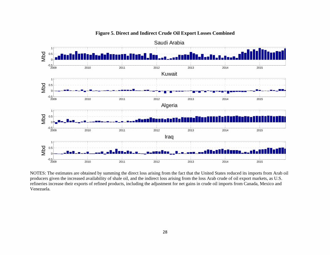
Figure 5 combines for each Arab oil producer the reduction in oil exports estimated in section 3
and that estimated in section 4. For Saudi Arabia, Algeria and Kuwait, there is a tendency for the export
losses expressed in million barrels of crude oil per day to increase over time. In the case of Saudi Arabia,
the combined losses reach one million barrels per day in 2014; Algeria reaches 0.5 million barrels per day
in 2013 and Iraq in 2015. Only Kuwait has been largely unaffected with no pronounced tendency for
6 These estimates were obtained by multiplying U.S. petroleum imports from these countries by the country-specific share of crude oil in these imports obtained from October 2014 data in the Energy Information Administration’s company level reports.

9
increased export losses over time. Aggregating these estimates across the four countries under
consideration, Arab oil exports losses over time reached a maximum of 5.3 mbd. This indirect estimate is
somewhat higher than the direct estimate of the increase in U.S. shale oil production in section 2.
5. How Much Oil Revenue Did Arab Oil Producers Lose?
So far we have quantified the physical oil exports foregone by Arab oil producers as a result of the surge
in U.S. tight oil production (measured in barrels per day). An equally important question is how large the
financial losses have been in U.S. dollars. For concreteness, my discussion in this section focuses on
Saudi Arabia. Answering this question involves constructing a counterfactual for the price of crude oil
based on a structural model of the global oil market. A natural question to explore is how different the
price of crude oil would have been, if all oil producers other than the United States had maintained their
observed oil production levels, but the U.S. fracking boom had never happened. This counterfactual level
of global oil production may be constructed either by lowering actual global oil production by the amount
of Arab oil export losses shown derived in sections 3 and 4 or alternatively by subtracting the direct
estimate of shale oil production in section 2. Given a suitable structural model of the oil market, one may
then infer the sequence of flow supply shocks required to produce this path of oil production after
November 2008, holding constant the remaining structural shocks in the model. If this counterfactual
shock sequence does not differ systematically from historical shock sequences, we may it back into the
structural model to simulate how the price of oil would have evolved under the counterfactual. Based on
this counterfactual price sequence, the implied increase in Saudi revenues may be computed as
, ( )Saudi actual counterfactual actualt t tQ P P , where ,Saudi actual
tQ denotes the observed level of Saudi oil production in
month t and counterfactual actualt tP P denotes the difference between the actual dollar price of oil and the dollar
price of oil obtained under this counterfactual.7
7 There are several potential caveats to keep in mind. First, this thought experiment is based on the premise that increased U.S. shale oil production was entirely due to exogenous oil supply shocks rather than being caused by oil demand shocks. This assumption is consistent with the view that in the absence of technological innovation, the shale oil boom would not have taken place, but it makes no allowance for effects working through oil price

10
5.1. The Structural Model of the Global Oil Market
The counterfactual price of oil is constructed with the help of a widely used structural vector
autoregressive (VAR) model of the global market for crude oil (see, e.g., Kilian and Murphy (2014);
Kilian and Lee (2014); Baumeister and Kilian (2014, 2016a)). This structural model includes four
variables: (1) the growth in global crude oil production, (2) a suitably updated measure of cyclical
fluctuations in global real economic activity originally proposed by Kilian (2009), (3) the log of the real
price of crude oil (obtained by deflating the U.S. refiners’ acquisition cost for crude oil imports by the
U.S. CPI), and (4) the change in above-ground global crude oil inventories measured by a suitable proxy.
We follow the literature in estimating the model at monthly frequency using seasonal dummies and 24
autoregressive lags. The model is re-estimated on data extending to August 2015, as described in Kilian
and Lee (2014). The structural shocks are identified based on a combination of sign restrictions and
bounds on the short-run price elasticities of oil demand and oil supply. The key identifying assumptions
are restrictions on the signs of the impact responses of the four observables to each structural shock.
There are four structural shocks. First, conditional on past data, an unanticipated disruption in the flow
supply of oil causes oil production to fall, the real price of oil to increase, and global real activity to fall
on impact. Second, an unanticipated increase in the flow demand for oil (defined as an increase in oil
demand for current consumption) causes global oil production, global real activity and the real price of oil
to increase on impact. Third, a positive speculative demand shock, defined as an increase in inventory
demand driven by expectations shifts not already captured by flow demand or flow supply shocks, in
equilibrium causes an accumulation of oil inventories and raises the real price of oil. The accumulation of
inventories requires oil production to increase and oil consumption to fall (associated with a fall in global
real activity). Finally, the model also includes a residual demand shock designed to capture idiosyncratic
oil demand shocks driven by a myriad of reasons that cannot be classified as one of the first three
expectations. Second, the counterfactual effectively postulates that Saudi Arabia would have been unable or unwilling to increase its oil production in the absence of the fracking boom.

11
structural shocks.8
As all sign-identified structural VAR models, this model is set-identified and does not yield a
unique solution. I follow Kilian and Lee (2104) in selecting the unique model that comes closest to a one-
month price elasticity of oil demand of -0.25, among all admissible solutions of the model. Figure 6
shows how much shocks to the flow demand for oil, to the flow supply of oil and to speculative (or
storage) demand shocks driven by oil price expectations have contributed cumulatively to the evolution of
the real price of oil, according to the model estimates. The estimates confirm that all three shocks
contributed to the decline in the real price of oil since June 2014 rather than the oil supply shock alone,
which is broadly consistent with the conclusions of Baumeister and Kilian (2016b) using an alternative
methodology.9
5.2. The Counterfactual Level of World Oil Production
Our main interest in this paper is in the sequence of flow supply shocks in the structural model. Given a
pre-specified counterfactual path of global oil production, we may infer the sequence of flow supply
shocks required to produce this path of oil production after November 2008, holding constant the
remaining structural shocks in the model. Similar techniques are discussed in Waggoner and Zha (1999)
and Baumeister and Kilian (2014). Knowledge of this sequence of flow supply shocks then allows us to
determine how much higher the price of oil would have been under this counterfactual compared with the
actual price of oil. A more detailed discussion of this procedure can be found in Appendix B.
Figure 7 shows two measures of the counterfactual path of world oil production corresponding to
competing views of how large world oil production would have been in the absence of the U.S. fracking
boom. The indirect measure in the left panel is derived from the effects of fracking on international trade
8 In addition to these static sign restrictions, the model imposes the dynamic sign restriction that structural shocks that raise the price of oil on impact do not lower the real price of oil for the first 12 months following the shock. The rationale for this restriction is that an unexpected flow supply disruption would not be expected to lower the real price of oil within the same year nor would a positive flow demand or speculative demand shock. Finally, the model imposes the restrictions that the impact price elasticity of oil supply is close to zero and that the impact price elasticity of oil demand cannot exceed the long-run price elasticity of oil demand, which conventional estimates put at -0.8. 9 Estimates of the responses of each model variable to each oil demand and supply shock are shown in Appendix A.

12
in crude oil. This measure consists of the reduction in U.S. crude oil imports from the rest of the world
and the crude oil equivalent of the increase in U.S. exports of refined products, adjusted for net increases
in U.S. crude oil imports from Canada, Mexico, and Venezuela, as discussed in sections 3 and 4. The
direct measure in the right panel is based on the change in shale oil production since November 2008, as
discussed in section 2. As noted earlier, the indirect measure is slightly larger than the indirect measure,
but the overall pattern is similar. One potential difference is that increased shale oil production need not
translate to increased production of refined products within the same month, given bottlenecks in the
shipping of this oil to U.S. refineries. Instead it may be accumulated in inventories and potentially refined
at a later point (see Kilian 2016). The indirect measure accounts for this problem and hence may be more
reliable. It may involve other approximation errors, however, that do not arise when constructing the
direct measure.
5.3. The Counterfactual Oil Supply Shock Sequences
Given the change in the quantity of oil produced in equilibrium under the counterfactual, it is
straightforward to infer how much the supply curve must shift each month, conditional on past data, in
order to produce the counterfactual equilibrium quantity. Figure 8 shows the sequence of flow supply
shocks that would have to be imposed in the global oil market model of Kilian and Lee (2014) to make
global oil production follow the counterfactual path of world oil production in Figure 7. An important
concern is whether the flow supply shocks required to implement the pre-specified path of global oil
production after November 2008 are too large by historical standards or too predictable to maintain the
assumption of a time-invariant structural VAR model. Figure 8 illustrates that neither of these shock
sequences involves shocks that are unusually large by historical standards, addressing the first concern.
As to the second concern that the counterfactual shocks must not be predictable, it is useful to focus on
evidence of a large number of consecutive flow supply shocks having the same sign (referred to as a
“run”). In the upper panel the longest run observed after December 2008 is seven months. Runs of this
length are not unprecedented. The longest run prior to December 2008, in fact, lasts nine months. Thus

13
runs in the flow supply shock data are neither particularly unusual nor do they necessarily imply that
market participants would have found it easy to anticipate these shocks. Rather their existence is
consistent with the view that the rapidly increasing growth rate of shale oil production continued to
surprise market participants more often than not. The corresponding shock sequence in the lower panel of
Figure 8, in contrast, exhibits one run lasting for fourteen months, which is considerably longer than the
longest run in the historical data, but similar runs are not unprecedented in other structural shock
sequences in this model and in the literature more generally. 10
5.4. How Much Higher the Brent Price Would Have Been Under the Counterfactuals
Figure 9 plots the Brent price of crude oil in U.S. dollars ( actualtP ) along with the counterfactual evolution
of the Brent price ( counterfactualtP ) based on these shock sequences. These estimates are obtained based on
counterfactual simulations of the log of the real price of oil in the global oil market model discussed
earlier, estimated on data until August 2015. The simulated oil price data have been suitably adjusted for
differences between the Brent price and the U.S. refiners’ acquisition cost for crude oil imports. The
Brent price of crude oil may be interpreted as a proxy for the global price of crude oil. The left panel of
Figure 9 shows that under the indirect measure of the counterfactual evolution of world oil production the
Brent price of oil would have been higher by as much as $5 in 2009, but most of the cumulative effects of
the fracking boom would have been observed between 2011 and mid-2014, with the counterfactual price
exceeding the actual Brent price by as much as $9 at times. Thereafter, the price differential
counterfactual actualt tP P becomes negligible again. In contrast, under the direct measure of the counterfactual
evolution of world oil production the Brent price of oil would have been largely the same as the actual
price until late 2010, as shown in the right panel of Figure 11. Between 2011 and mid-2014, the Brent
price of oil would have been higher by as much as $10 in the absence of the U.S. fracking boom, reaching
$120 repeatedly and at some point even $130. Unlike in the first counterfactual, even in 2015, the Brent
10 In a related context, Kilian and Hicks (2013) documented prediction errors in professional global real GDP growth forecasts of the same sign for nearly five years during 2003-08. As long as such patterns average out in the long run, they do not violate the premise of rational expectations.

14
price would have been higher than actually observed price by as much as $5. 11
The estimates in Figure 9 also shed light on the extent to which the U.S. fracking boom caused
the decline in the global price of crude oil in late 2014 and early 2015. Both counterfactuals agree that in
the absence of the fracking boom this oil price decline would have occurred at the same time, as it did, but
that it would have started at a higher level. According to Figure 9, the cumulative decline in the Brent
price would have been $70 under both specifications of the counterfactual (and therefore would have been
$6 higher than in the actual data). Thus, there is no support for the view that U.S. fracking was the
primary cause of this specific oil price decline. This result complements the analysis in Baumeister and
Kilian (2016b) who were unable to pin down the quantitative role of fracking specifically, but who
provided evidence that a slowdown in the global demand for oil was a major contributor to this specific
oil price decline in addition to a mix of shocks to actual and/or expected global oil supplies prior to July
2014 and a shift in oil price expectations in July 2014. Figure 9 helps refine that interpretation. It also
complements the analysis of the cumulative impact of all global oil supply shocks combined in Figure 6
based on the structural model of Kilian and Lee (2014).
5.5. Choosing Among the Two Counterfactuals
The first two panels of Figure 10 show the price differentials counterfactual actualt tP P obtained from Figure 9
under each of the two alternative counterfactuals. It highlights that only the indirect measure implies a
positive price differential during 2009 and early 2010, whereas only the direct measure implies a positive
price differential after late 2014, raising the question of which of these price differentials is economically
more plausible. This question may be assessed based on the information in the bottom panel of Figure 10,
which plots the dollar spread between the Brent price and the West Texas Intermediate (WTI) price of
11 The order of magnitude of the estimated cumulative effects seems reasonable in light of historical evidence on the effect of oil supply shocks. When the Iran-Iraq War broke out in late 1980, about 4% of world oil production was removed from the market, followed by approximately a 10% increase in the price of crude oil. U.S. shale oil production amounts to an increase of about 4% in global crude oil production, as shown in Kilian (2016), and hence would be expected to be associated with a fall in the price of oil of about 10%, which amounts to about $10 per barrel.

15
crude oil.12 This spread conveys important information about when the fracking boom began to affect the
U.S. market for crude oil.
The fact that the Brent-WTI spread only widened in late 2010 suggests that the positive price
differential during 2009 and early 2010 in the first panel cannot be attributed to the fracking boom,
casting doubt on the indirect counterfactual. As discussed in Kilian (2016), traditionally these crude oil
prices have been closely tracking one another. This pattern only changed when the U.S. tight oil boom
created a glut of crude oil in the central United States, causing WTI oil to trade at a discount relative to
the global price for oil, as measured by the Brent price. We know that the initial drop in the WTI price
relative to the Brent price occurred because there was not enough transportation capacity to ship the crude
oil arriving from the Bakken and other shale oil plays in large enough quantities from Cushing to refiners
elsewhere in the United States. As a result, most U.S. refiners, including the refiners along the Gulf Coast
and the East Coast, continued to rely on oil imports at this stage (see Kilian 2016). Nor were U.S. refiners
able to take advantage of the glut of oil in Cushing to increase exports of refined products. These
transportation bottlenecks loosened only gradually over time, as rail, barge and pipeline capacity
increased. There are of course shale oil plays such as Eagle Ford in Texas with easier access to refineries
in the Houston area and beyond, but production in Eagle Ford was negligible prior to 2011. Given that
neither of the two mechanisms by which shale oil production affects the global price of oil were in
operation at this stage of the shale oil boom, it would be unreasonable to expect shale oil production to
have had a large effect on the global price of crude oil before 2011. In short, the evolution of the Brent-
WTI spread supports the conclusion that the price differential in the second panel based on the direct
measure of the counterfactual is a more accurate approximation. The remainder of the analysis therefore
focuses exclusively on the latter counterfactual.13
12 The Brent price refers to the spot price of light sweet crude oil traded in London, UK, whereas the WTI price is the spot price of light sweet crude oil for delivery in Cushing, OK. 13 It is important to stress that the Brent-WTI price differential does not by itself represent a proper counterfactual for the global price of oil because an increase in tight oil production all else equal will have a larger effect on the U.S. price of oil than on the global price. All we can say is that if there is no effect on the U.S. price of oil until late 2010, then fracking is unlikely to have affected the global price before this point in time. The evolution of the Brent-

16
5.6. Implications for Saudi Oil Revenue
The sequence of price differentials counterfactualtP actual
tP may be used to compute, month by month from
December 2008 until August 2015, the additional revenue Saudi Arabia would have received after
November 2008 in the absence of the U.S. fracking boom, given the historically observed levels of Saudi
oil production. The upper panel of Figure 11 shows the evolution of the losses in Saudi oil revenue
measured in billions of U.S. dollars under the preferred counterfactual based on the direct measure of
tight oil production. There is evidence that the Saudi oil revenue losses were negligible initially, but
gradually increased over time, reaching 2 billion dollar per month in late 2012 and peaking at 2.9 billion
dollars per month in mid-2014, before levelling off. Of course, this evidence does not speak to the overall
loss of Saudi oil revenue following the decline in the price of oil after June 2014, but only to the
component of this loss caused by the U.S. fracking boom. It should also be noted that the dip in Saudi oil
revenue losses in January 2015 mirrors the temporary tightening of the Brent-WTI spread, adding
credibility to this estimate.
A rough measure of the cumulative impact of the fracking boom on Saudi Arabia is obtained by
simply cumulating these losses. The cumulative decline in Saudi oil revenue between December 2008 and
August 2015 is 102.1 billion dollars. This amounts to an average loss per month of 1.3 billion U.S.
dollars. The incremental Saudi oil revenue losses between July 2014, when the price of oil began to fall
precipitously, and August 2015 are 24.3 billion dollars. To put these estimates in perspective, the lower
panel of Figure 13 expresses the reduction in Saudi oil revenues caused by the fracking boom as a
percentage of the Saudi oil revenue in November 2008, when the Brent price of oil stood at $52.45. It is
important to be clear about the interpretation of this estimate. Figure 13 shows that in mid-2014, for
example, Saudi Arabia in the absence of the U.S. fracking boom would have earned 120% of the oil
revenue it generated in November 2008, if it had produced exactly as much oil as it actually did in mid-
2014. In other words, the plot does not measure the actual change in the oil revenue generated by the WTI spread between 2011 and 2014, in contrast, tells us little about the counterfactual for the global price because it reflects in important part the evolution of transportation and refining bottlenecks in the United States (see Kilian 2016).

17
Saudi economy, but rather the lost revenue relative to what Saudi Arabia would have earned if the United
States still relied on conventional crude oil production only.14
6. Concluding Remarks
Saudi Arabia’s strategy for dealing with the fracking boom so far has been to preserve its market share
and to avoid idle capacity (see, e.g., Fattouh and Sen 2015; Fattouh, Poudineh and Sen 2015). There is no
sign of Saud Arabia curtailing its oil production nor is it likely that such a strategy would help preserve
Saudi oil revenue (see Baumeister and Kilian 2016b). Instead, the Saudi government has dealt with the
decline in its oil revenue mainly by tapping its financial reserves, as predicted by standard models of
precautionary savings (see, e.g., Bems and de Carvalho Filho 2011). IMF data show a reduction in Saudi
net foreign asset holdings of near $90 billion between mid-2014 and August 2015. This estimate is
considerably larger than the loss in oil revenue over the same period that is attributable to the fracking
boom. The latter we estimated to be about $24 billion. In other words, the analysis in this paper
tentatively suggests that in the absence of the fracking boom the reduction in Saudi foreign exchange
reserves since mid-2014 would have been about two thirds of the actual decline with the remainder
reflecting higher crude oil production elsewhere in the world, shifts in oil price expectations affecting the
demand for oil stocks, and the effects of a slowing global economy.
An important question is how long Saudi Arabia can sustain such losses in its foreign exchange
reserves. If the decline in Saudi net foreign assets were to continue at the rate experienced between
January 2015 and January 2016, one would expect Saudi net foreign assets to be exhausted by early 2020.
14 It should be kept in mind that this estimate is only an approximation, first, because Saudi oil exports that were diverted from the United States to Asian economies, for example, were not necessarily priced based on the Brent benchmark, and, second, because my methodology abstracts not only from changes in Saudi oil production, but also from any Saudi efforts to market its oil more aggressively. With regard to the first point, my analysis assumes that the price of Saudi crude oil declined as much as the price of Brent crude, allowing for differences in the level of these prices. My analysis also abstracts from differences between Saudi exports of heavy and light crude oil. The concern is not so much that Saudi Arabia could have substituted exports of heavy crude to the United States for its exports of light crude. This possibility seems unlikely because, as I showed, imports of lower-priced Canadian heavy crudes increasingly substituted for U.S. imports of heavy crudes from other sources, at the same time as shale oil production displaced U.S. imports of light sweet crude oil. Rather the concern is that by applying the counterfactual price differential indiscriminately to Saudi production of light and heavy crude oil, one overestimates the loss in oil revenue that can be attributed to shale oil because shale oil competes with Saudi heavy crude oil only indirectly through U.S. exports of refined products.

18
Of course, this process would accelerate if the price of oil were to fall further, or it would slow if the price
were to recover somewhat. There are two potential mitigating factors, however. First, unlike some of its
neighbors, Saudi Arabia has very little external debt because it resisted the temptation to leverage its
increased oil revenues during the 2003-08 oil price boom by running up external debt (see Tornell and
Lane 1998). As a result, for now, the Saudi government has been able to borrow in global financial
markets, given the expectation that the price of oil will ultimately recover. Second, the Saudi government
thus far has been reluctant to impose fiscal retrenchment, because of the political costs of such measures,
but in December 2015 it announced a budget plan that envisions cuts in spending from $975 billion in
2015 to $840 billion in 2016 (representing a 14% drop in government spending). The finance ministry
also announced that it would raise taxes and adjust subsidies for water, electricity and petroleum products
over the next five years.
The central question for Saudi Arabia is to what extent it should rely on external borrowing and
to what extent it should cut fiscal spending. Economic theory tells us that it makes sense for Saudi Arabia
to borrow in response to a short-lived fall in oil prices. If the decline in the price of oil were expected to
persist for a long time, in contrast, external borrowing would not be the appropriate response and the
adjustment instead would have to come from fiscal retrenchment. Thus, the answer to the question of
how much fiscal adjustment Saudi Arabia requires is ultimately determined by how long one expects low
oil prices to persist. How soon the price of oil is expected to recover depends in important part on why the
price of oil declined and how important these determinants will remain in the future (see Baumeister and
Kilian 2016b).
For example, to the extent that this price decline was caused by the U.S. fracking boom, the
question is how long this boom can persist at current prices with many commercial tight oil producers
already experiencing heavy operating losses, and how quickly these firms could resume tight oil
production at higher oil prices, if they were forced to close down. The same concern applies to
unconventional oil production in Canada. Even if the current low price of oil were to put shale oil
producers out of business, however, an obvious concern would be that shale oil production is likely to

19
resume as soon as world oil prices recover sufficiently, as long as there remains easily accessible shale oil
in the ground. At $60 per barrel, for example, many U.S. shale oil producers are likely to generate
profits, even if they do not at $40 per barrel. If we accept this reasoning, we should treat much of the
shale oil component of the Saudi foreign exchange losses as persistent and respond by cutting Saudi fiscal
spending rather than borrowing.
Of course, shale oil is only one reason for the ample supply of crude oil in world markets. To the
extent that other oil producers including Russia and Iraq have expanded oil production in recent years, or,
as in the case of Iran, are about to do so, the question becomes one of how long state-controlled oil
producers with few other options to generate foreign exchange and no accountability to shareholders or
financial markets will put pressure on the price of oil. Countries such as Russia, for example, rely on oil
revenue both to finance their military ambitions and to sustain the domestic economy. There is no reason
to expect these countries to reduce their exports, except to the extent that inadequate investment in the oil
sector limits their ability to sustain high levels of oil production in the long run.
One countervailing force on the supply side is that production in many other oil-producing
countries will continue to fall over time, as conventional fields are depleted. The United Kingdom and
Norway are good examples. There also examples of oil producers such as Mexico, where mismanagement
has made oil production too costly to compete in global markets. These high costs in conjunction with
low investment have slowed Mexican oil production. Table 1 documents that world oil production has not
grown nearly as fast, as might have been suggested by news reports about rising oil production in selected
countries. The simultaneous gradual decline in oil production elsewhere in the world has largely gone
unreported. Over time one would expect these continued production declines to make room for higher oil
production in countries such as Iraq, Iran, Saudi Arabia, Russia, or the United States. The problem from
Saudi Arabia’s point of view is that there is a good chance that this process may take longer than its net
foreign assets will last.
One would, in fact, expect this gradual decline in global oil production to be accelerated by the
current worldwide cutbacks in investment in oil exploration and new oil fields. As a result, it would be

20
surprising if the price of crude oil did not recover somewhat over the next few years. Just how far this
cyclical effect will push up the price of oil and how soon is less clear, however. It may easily take another
year or two for these effects to become quantitatively important. Moreover, a partial recovery of the
global price of crude oil to $65 per barrel in, say, two years would still leave the Saudi economy facing a
substantial shortfall compared with prices near $110 per barrel prior to July 2014.
The demand side of the oil market also plays an important role in assessing the persistence of the
current oil price slump. To the extent that low oil prices reflect a sluggish global economy, as shown in
Figure 8, the question becomes at what point emerging Asia, Japan, and Europe, in particular, will
recover. A swift and sustained global economic recovery, unlikely as it may seem at this point, would
quickly eliminate the current glut of crude oil. All indications are, however, that there remains
considerable downside risk in the global economy and that the global recovery, when it starts, is likely to
be slow and gradual. One would not expect the demand for oil to surge in the foreseeable future.
A final remedy may seem to be coordinated oil supply cuts, which helped alleviate the glut of
crude oil in 1998, when the price of oil dropped to $11 (see Kilian and Murphy 2014). That solution
seems unlikely in the current environment of low demand for oil, however, if we take the theory of cartels
as a guide. Oil cartels are inherently procylical and tend to fall apart during economic slumps (see Barsky
and Kilian 2002). Notwithstanding recent talks between Venezuela, Saudi Arabia, Russia and other oil
producers about coordinated supply restrictions, all indications are that these producers are more likely to
freeze recent high production levels than to agree on actual production cuts. Moreover, the United States,
Iran and Iraq are unlikely to feel bound by any such agreements, undermining any potential agreements.
There is little doubt that the price of oil will recover in the longer run, but the question is whether
Saudi net foreign assets can sustain the Saudi economy until then. It is more than likely that the Saudi
economy could face another three or four lean years, at which point the precautionary savings in the Saudi
sovereign wealth fund would likely be exhausted, while the prospects of new external borrowing would
diminish. Already, the Saudi credit rating has been lowered. Thus, there appears to be no alternative to
some considerable measure of fiscal retrenchment in the foreseeable future. The same argument applies

21
even more forcefully to other Arab oil producers faced with more foreign debt and lower foreign
exchange reserves.
A natural starting point for such reforms would be for policymakers to reduce or even phase out
domestic subsidies on energy consumption. In fact, implementing such reforms is likely to be easier
politically in an environment of falling oil prices. The United Arab Emirates, for example, have already
successfully aligned their domestic fuel prices with prices in global markets. Many other Arab oil
producers have yet to implement similar reforms. Clearly, however, such reforms will not be enough,
given the magnitude of the oil revenue shortfall that has accumulated in recent years. There will have to
be more fundamental changes to the welfare state in countries such as Saudi Arabia and implementing
these changes will be politically challenging. One problem is that many Arab oil producing countries
lack an income tax base. Taxing incomes of domestic citizens working in the public sector would be the
same effectively as lowering public wages and hence fiscal spending, leaving taxes on foreign workers’
income as the only policy option for raising tax revenue. Thus, much of the fiscal adjustment will have to
occur on the expenditure side. It seems safe to conclude that an extended period of low oil prices is likely
to cause far-reaching economic changes in Arab oil producing countries as well as changes in the social
fabric, whether these changes are implemented gradually in anticipation of growing financial constraints
or are eventually forced by external events. The obvious concern is that, if this transition is not managed
well, geopolitical risks in the Middle East, which have not played a large role since 1990, may become
much more important again, contributing to higher oil prices in the long run.
References
Barsky, R.B., and L. Kilian (2002), “Do We Really Know that Oil Caused the Great Stagflation? A
Monetary Alternative,” in: B. Bernanke and K. Rogoff (eds.), NBER Macroeconomics Annual
2001, 137-183.
Baumeister, C., and L. Kilian (2014), “Real-Time Analysis of Oil Price Risks using Forecast Scenarios,”
IMF Economic Review, 62, 119-145.
Baumeister, C., and L. Kilian (2016a), “Forty Years of Oil Price Fluctuations: Why the Price of Oil

22
May Still Surprise Us,” Journal of Economic Perspectives, 30, 139-160.
Baumeister, C., and L. Kilian (2016b), “Understanding the Decline in the Price of Oil since June 2014,”
Journal of the Association of Environmental and Resource Economists, 3, 131-158Bems, R.,
and I. de Carvalho Filho (2011), “The Current Account and Precautionary Savings for
Exporters of Exhaustible Resources,” Journal of International Economics, 84, 48-64.
Benes, J., Chauvet, M., Kamenik, O., Kumhof, M., Laxton, D., Murula, S., and J. Selody (2015), “The
Future of Oil: Geology versus Technology,” International Journal of Forecasting, 31, 207-
221.
Coglianese, J., Davis, L.W., Kilian, L., and J.H. Stock (2016), “Anticipation, Tax Avoidance, and the
Price Elasticity of Gasoline Demand,” forthcoming: Journal of Applied Econometrics.
Fattouh, B. (2014), “The U.S. Tight Oil Revolution and its Impact on the Gulf Cooperation Council
Countries: Beyond the Supply Shock,” OIES Paper WPM 54, Oxford Institute of Energy
Studies.
Fattouh, B. and A. Sen (2015), “Saudi Arabia Oil Policy: More than Meets the Eye?”, OIES Paper
MEP 13, Oxford Institute of Energy Studies.
Fattouh, B., Poudineh, R., and A. Sen (2015), “The Dynamics of the Revenue Maximization-Market
Share Trade-Off: Saudi Arabia’s Oil Policy in the 2014-2015 Price Fall”, OIES Paper WPM
61, Oxford Institute of Energy Studies.
Holland, S.P. (2008), “Modeling Peak Oil,” Energy Journal, 29, 61-80.
Holland, S.P. (2013), “The Economics of Peak Oil,” in: Shogren, J.F. (ed.), Encyclopedia of
Energy, Natural Resource, and Environmental Economics, Vol. 1, Amsterdam: Elsevier, 146-
150.
Kilian, L. (2009), “Not All Oil Price Shocks Are Alike: Disentangling Demand and Supply Shocks in
the Crude Oil Market”, American Economic Review, 99, 1053-1069.
Kilian, L. (2016), “The Impact of the Shale Oil Revolution on U.S. Oil and Gas Prices,” forthcoming:
Review of Environmental Economics and Policy.
23
Kilian, L., and B. Hicks (2013), “Did Unexpectedly Strong Economic Growth Cause the Oil Price
Shock of 2003-2008?” Journal of Forecasting, 32, 385-394.
Kilian, L., and D.P. Murphy (2014), “The Role of Inventories and Speculative Trading in the
Global Market for Crude Oil,” Journal of Applied Econometrics, 29, 454-478.
Kilian, L., and T.K. Lee (2014), “Quantifying the Speculative Component in the Real Price of Oil:
The Role of Global Oil Inventories,” Journal of International Money and Finance, 42, 71-87.
Tornell, A., and P. Lane (1998), “Are Windfalls a Curse? A Non-Representative Agent Model of the
Current Account,” Journal of International Economics, 44, 83-112.
U.S. Energy Information Administration (2015), Monthly Energy Review, December.
U.S. Energy Information Administration (2016), Drilling Productivity Report, January.
Waggoner, D.F., and T. Zha, (1999), “Conditional Forecasts in Dynamic Multivariate Models,” Review of
Economics and Statistics, 81, 639-651.
Table 1. Changes in Crude Oil Production
2008.11-2015.9 2014.6-2015.9 Oil producers
Change in million
barrels/day
Average percent change1
Change in million
barrels/day
Average percent change1
World 6.17 1.16 2.76 2.63 Saudi Arabia 1.23 1.86 0.50 3.78 Other Persian Gulf 1.97 2.08 1.14 6.05 Iran -0.80 -3.13 0.15 3.49 Iraq 2.07 9.12 1.10 21.63 Kuwait 0.06 0.37 -0.10 -2.88 Qatar 0.36 3.90 -0.02 -0.78 UAE 0.25 1.39 0 0 Russia 0.79 1.17 0.06 0.41 Canada and United States 5.03 7.24 0.57 3.44 Canada 0.73 3.48 -0.14 -2.93 United States 4.30 8.89 0.71 5.91
Source: U.S. Energy Information Administration (2105), Monthly Energy Review. Notes: 2008.11 marks the reversal in the long-term decline of U.S. oil production. 2014.6 marks the end of a long period of relative price stability in the market of crude oil, before the recent collapse of the price of crude oil (see Baumeister and Kilian 2016). 1 at annualized rates
24
1994 1996 1998 2000 2002 2004 2006 2008 2010 2012 20140
2
4
6
8
10
12
14
16
Mill
ion
barr
els/
day
Oil Production by Country
2008 2009 2010 2011 2012 2013 2014 2015 20160
1
2
3
4
5
6U.S. Shale Oil Production
Mill
ion
barr
els/
day
United StatesCanadaRussiaSaudi ArabiaOther Persian Gulf
Figure 1. Crude Oil Production Disaggregated
NOTES: The international data are from U.S. Energy Information Administration (2015). The production data are for crude oil and lease condensate, but exclude natural gas plant liquids. The vertical line marks the reversal in the long-term decline of U.S. oil production in November 2008. The shale oil production data are obtained from U.S. Energy Information Administration (2016) by adding crude oil production in the seven largest U.S. shale oil plays, which account for the bulk of U.S. shale oil production.

25
1975 1980 1985 1990 1995 2000 2005 2010 20150
2
4
6
8
10
12
14
16
Mill
ion
barr
els/
day
Production and Trade
ProductionImportsExports
1975 1980 1985 1990 1995 2000 2005 2010 20150
2
4
6
8
10
12
14
16
Mill
ion
barr
els/
day
Total Oil Use
Figure 2. The U.S. Crude Oil Sector, 1973.1-2015.11
NOTES: The raw data are from U.S. Energy Information Administration’s (2015). Total oil use is defined as: Domestic Production of Crude Oil + Crude oil imports – Crude oil exports.

26
1975 1980 1985 1990 1995 2000 2005 2010 20150
10
20
30
40
50
60
70
80
90
100
Per
cent
of U
.S. O
il U
se
Import Shares by Subaggregates
2005 2006 2007 2008 2009 2010 2011 2012 2013 2014 20150
2
4
6
8
10
12
14
16
18
Per
cent
of U
.S. O
il U
se
Import Shares of Arab Oil Producers
Total importsImports from OPECImports from Arab OPEC (excl. Libya)Imports from West Africa
Imports from Saudi ArabiaImports from KuwaitImports from AlgeriaImports from Iraq
Figure 3. Crude Oil Imports from Selected Countries as a Percent Share of U.S. Oil Use
NOTES: The raw data are from U.S. Energy Information Administration (2015). The vertical line marks the reversal in the long-term decline of U.S. oil production in November 2008.It also coincides with the drop of the share of Saudi oil imports in the U.S. use of oil.

27
1975 1980 1985 1990 1995 2000 2005 2010 20150
0.5
1
1.5
2
2.5
3
3.5
4
4.5
5
Mill
ion
barr
els/
day
U.S. Exports of Refined Products
ActualCounterfactual
2009 2010 2011 2012 2013 2014 20150
0.5
1
1.5
2
2.5
3
3.5
4
4.5
5
Mill
ion
barr
els/
day
Crude Oil Equivalent of Exports Lost by Other Producers
BaselineExcluding Canada Effect
Figure 4. Quantifying the Displacement of Other Crude Oil Producers’ Exports Caused by U.S. Exports of Refined Products
NOTES: Based on data from U.S. Energy Information Administration (2015). The vertical line marks the reversal in the long-term decline of U.S. oil production in November 2008. The counterfactual is constructed by assuming that the share of U.S. exports of refined products in total use of oil by the U.S. economy remains constant at its level in November 2008. The crude oil equivalent is computed by multiplying the shortfall of exports computed in the left panel by 1.3548. This conversion factor is based on the fact that U.S. refineries in 2014 on average produced 12 gallons of diesel and 19 gallons of gasoline (for a total of 31 gallons of refined product) from 42 gallons (one barrel) of crude oil, according to the EIA. The Canada effect refers to increased imports of crude oil from Canada in excess of the reduction of U.S. imports of crude oil from Mexico and from Venezuela. To isolate U.S. exports of refined products made from domestic crude oil, this effect must be corrected for.
28
2009 2010 2011 2012 2013 2014 2015-0.5
0
0.5
1Saudi Arabia
Mbd
2009 2010 2011 2012 2013 2014 2015-0.5
0
0.5
1Kuwait
Mbd
2009 2010 2011 2012 2013 2014 2015-0.5
0
0.5
1Algeria
Mbd
2009 2010 2011 2012 2013 2014 2015-0.5
0
0.5
1Iraq
Mbd
Figure 5. Direct and Indirect Crude Oil Export Losses Combined
NOTES: The estimates are obtained by summing the direct loss arising from the fact that the United States reduced its imports from Arab oil producers given the increased availability of shale oil, and the indirect loss arising from the loss Arab crude of oil export markets, as U.S. refineries increase their exports of refined products, including the adjustment for net gains in crude oil imports from Canada, Mexico and Venezuela.

29
Figure 6. Cumulative Effect of Oil Demand and Oil Supply Shocks on the Real Price of Oil NOTES: The underlying structural model is constructed as in Kilian and Lee (2014), except the estimation sample has been updated to August 2015. The real price of oil is expressed in percent deviations from the long-run average real price of crude oil. Each subplot shows the extent to which the shock in question moved the real price of oil up or down since 2003. The vertical lines mark the beginning of the oil price decline of 2014-15.

30
1975 1980 1985 1990 1995 2000 2005 2010 201545
50
55
60
65
70
75
80
85
Mill
ion
barr
els/
day
ActualCounterfactual 2: Indirect Measure
1975 1980 1985 1990 1995 2000 2005 2010 201545
50
55
60
65
70
75
80
85
Mill
ion
barr
els/
day
ActualCounterfactual 2: Direct Measure
Figure 7. Alternative Counterfactuals for World Oil Production in the Absence of the U.S. Fracking Boom
NOTES: The indirect counterfactual is based on the losses in crude oil exports of the rest of the world caused by a reduction in U.S. crude oil imports and the expansion of U.S. exports of refined products, adjusted for the net increase in U.S. crude oil imports from Canada, Mexico, and Venezuela, representing primarily an influx of heavy crudes unrelated to fracking. The direct counterfactual is derived on an estimate of the change in U.S. shale oil production since 2008.11, as shown in the right panel of Figure 1.

31
1980 1985 1990 1995 2000 2005 2010 2015-5
0
5Indirect Measure
1980 1985 1990 1995 2000 2005 2010 2015-5
0
5Direct Measure
Figure 8. Sequence of Flow Supply Shocks Required to Implement the Alternative Counterfactuals in Figure 8
NOTES: Computations by the author based on the algorithm described in Appendix B. The vertical line marks the beginning of the counterfactual in December 2008.

32
2009 2010 2011 2012 2013 2014 20150
20
40
60
80
100
120
140
U.S
. Dol
lars
Direct Measure
CounterfactualActual
2009 2010 2011 2012 2013 2014 20150
20
40
60
80
100
120
140
U.S
. Dol
lars
Indirect Measure
CounterfactualActual
Figure 9. The Impact of Shale Oil Production on the Brent Price of Crude Oil
NOTES: The counterfactual path for the nominal Brent price of crude oil inferred from the two counterfactuals in Figure 7, as discussed in Appendix B.

33
2009 2010 2011 2012 2013 2014 2015-10
0
10
20
30Price Differential: Direct Measure
U.S
. Dol
lars
2009 2010 2011 2012 2013 2014 2015-10
0
10
20
30Brent-WTI Price Differential
U.S
. Dol
lars
2009 2010 2011 2012 2013 2014 2015-10
0
10
20
30Price Differential: Indirect Measure
U.S
. Dol
lars
Figure 10. Brent Oil Price Differentials
NOTES: The first two panels are constructed from the counterfactual price paths for the Brent price in Figure 9. The third panel shows the spread between the Brent and WTI spot prices, as reported by the EIA.

34
2009 2010 2011 2012 2013 2014 2015-2
0
2
4
6
8
Oil Revenue LossesB
illion
US
$
2009 2010 2011 2012 2013 2014 2015-20
0
20
40
60
80
100Oil Revenue Losses Relative to Saudi Oil Revenue of November 2008
Perc
ent
Figure 11. Saudi Oil Revenue Losses Under the Direct Measure of the Counterfactual
NOTES: The plot in the lower panel expresses the reduction in Saudi oil revenues caused by the fracking boom as a fraction of Saudi oil revenue in November 2008, when the Brent price of oil stood at $52.45. For example, at its peak in 2014 the oil revenue loss amounted to 20% of the Saudi oil revenue of November 2008.

35
0 5 10 15-2
-1
0
1
Oil
prod
uctio
n
Flow supply shock
0 5 10 15-5
0
5
10
Rea
l act
ivity
Flow supply shock
0 5 10 15-5
0
5
10
Rea
l pric
e of
oil Flow supply shock
0 5 10 15-40
-20
0
20
40
Inve
ntor
ies
Flow supply shock
0 5 10 15-1
0
1
2
Oil
prod
uctio
n
Flow demand shock
0 5 10 15-5
0
5
10R
eal a
ctiv
ityFlow demand shock
0 5 10 15-5
0
5
10
Rea
l pric
e of
oil Flow demand shock
0 5 10 15-40
-20
0
20
40
Inve
ntor
ies
Flow demand shock
0 5 10 15-1
0
1
2
Oil
prod
uctio
n
Months
Speculative demand shock
0 5 10 15-5
0
5
10
Rea
l act
ivity
Months
Speculative demand shock
0 5 10 15-5
0
5
10
Rea
l pric
e of
oil
Months
Speculative demand shock
0 5 10 15-40
-20
0
20
40
Inve
ntor
ies
Months
Speculative demand shock
Appendix A: Responses of the Global Oil Market VAR Model Variables to Each of the Structural Shocks
NOTES: The underlying model is constructed as in Kilian and Lee (2014), except the estimation sample has been updated to August 2015. All responses but the inventory responses are expressed in percentages. The inventory responses are in million barrels.

36
Appendix B: Constructing the Oil Price Series under Counterfactual 2
Let 1 2 3 4( . , , ) 't t t t ty y y y y denote the vector of variables in the global oil market model of Kilian and
Murphy (2014), where 1ty stands for the growth in world oil production and 3ty for the log of the real
price of oil, in particular. Consider the structural VAR model
0 1 1 24 24... ,t t t tB y B y B y w (1)
where the 4 1 vector ty is assumed to be stationary and the deterministic regressors have been
suppressed for expository purposes. The dimension of , 0,...,24,iB i is 4 4. The 4 1 vector of
structural shocks, 1 2 3 4( , , , ) ',t t t t tw w w w w where 1tw denotes a shock to the flow supply of crude oil, is
assumed to be zero mean white noise with a diagonal 4 4 variance-covariance matrix w that is of full
rank and that without loss of generality can be normalized to equal the identity matrix. This structural
model can be expressed in its reduced form as
1 1 24 24... ,t t t ty A y A y u (2)
where 10 , 1,...,24,i iA B B i and 1
0t tu B w with variance-covariance matrix 1 10 0( ) .u B B Let the
4 4 matrix /t i t iy w denote the responses of the model variables to each of the structural shocks
at horizon 0,1,..., .i H The matrix ,i jk i consists of elements , , /jk i j t i kty w that denote the
response of variable j to structural shock k at horizon .i These responses may be computed as
10' ,i
i J J B A where 4 4 4(24 1)0J I and A denotes the matrix of slope parameters obtained by
expressing the VAR(24) reduced-form model in its VAR(1) companion format.
In constructing the counterfactual in question, we make use of the fact that after removing the
deterministic terms
1
0
.t
t i t ii
y w
As a result, the fitted value for the log real price of oil can be written as

37
( )4
3 1 3ˆ ˆ ,
j
t j ty y
(3)
where ( )3ˆ j
ty denotes the cumulative contribution since the beginning of the sample of structural shock j to
the third model variable at time ,t defined as
1(1)3 31, 1,0
1(2)3 32, 2,0
1(3)3 33, 3,0
1(4)3 34, 4,0
ˆ ,
ˆ ,
ˆ ,
ˆ .
t
t i t ii
t
t i t ii
t
t i t ii
t
t i t ii
y w
y w
y w
y w
Having simulated the posterior of the reduced-form model (2) obtained based on the full sample from
February 1973 to August 2015, we recover estimates of 10 ,B
,jk i and of 0 , 1,..., ,t tw B u t T as in Kilian
and Lee (2014) by selecting the posterior model with a short-run price elasticity of oil demand closest to
the benchmark estimate of -0.26 in the literature (see Kilian and Murphy 2014; Coglianese et al. 2016).
In constructing the counterfactual, we retain the realizations of the flow supply shock 1,tw up to
November 2008, but we replace the estimates of 1,tw for December 2008.12 through August 2015 by
counterfactual values chosen to ensure that the path of world oil production corresponds to the
counterfactual path shown in Figure 9. Given the demeaned growth rate of world oil production implied
by the counterfactual, these values may be easily computed by an iterative procedure. Having computed
what the expected value of 1ty given ( )1ˆ , 2,3,4,jty j would have been next month, if this month’s supply
shock had been zero, the difference between that model prediction and the target level of oil production
growth, scaled by the impact response of world oil production to a flow supply shock, will be the
magnitude of the flow supply shock, 1 ,tw required to reach the growth target.
We then recompute (1)3ˆ ty under the alternative sequence of flow supply shocks, while retaining the
other three structural shock sequences as originally estimated in computing (2)3ˆ ,ty (3)
3ˆ ty and (4)3ˆ .ty Given
the implied sequence of 3ˆ ,ty the corresponding sequence counterfactualtP is constructed from the real price of

38
Brent crude oil, scaled up by the percent deviation between the counterfactual real price of oil and the
actual real price of oil in the model. The counterfactual real Brent price is converted back to dollars using
the U.S. consumer price index. The price differential counterfactual actualt tP P for the remainder of the sample
is obtained by subtracting the actual dollar price of Brent crude oil, ,actualtP from .counterfactual
tP