The impact of the Institutions on Regional Unemployment disparities Floro Ernesto Caroleo, Gianluigi Coppola

caroleo, glcoppola@unisa.it (Celpe, Centro Interdipartimentale di Economia del Lavoro e di Scienze Economiche

DISES, Dipartimento di Scienze Economiche e Statistiche )

Abstract

The main aim of this paper is to study the European regional disparities in the labour market,

considering the regional productive structures and some regional institutional variables. It is

widely known that one of the EU’s most important stylized facts are the regional disparities

among regions. Such differences are related mostly to the income per capita and to the labour

market captured through the unemployment rates. In a recent paper (Amendola, Caroleo

Coppola, 2004) we analyzed the economic structure of the EU’s regions through some proxies

of the productive assets and of the labour markets. In this paper we estimate a Panel data where

the dependent variable is the regional unemployment rate and the independent variables are

some variables related to the productive structure and some regional institutional aspects. The

results we obtain confirm that the institutional variables, such as the centralization of wage

bargaining, the decentralization of public expenditure and the bureaucracy level, play an

important impacts on the unemployment rates.

JEL CODES: R23, C23, H70

Introduction

The problem of the regional disparities is a crucial theme in the debate on the economic and politic

process of the construction of the European Union. In fact if we compare the United States with the

European Union, we find that the convergence process is slower in the Old Continent. Moreover in

the same periods the disparities among regions persist or increase.

1

As a matter of fact it is possible to find many examples about the persistence of the regional

disparities: the unsolved problem of the German unification (Marani, 2004), the absence of growth

for many less-developed regions in the Mediterranean Europe (Caroleo e Destefanis 2005), the slow

transition of the East European countries (Perugini e Signorelli 2004).

The implications for the economic theory and for the policy issues are very important. In fact there

is not a growth theory so far, as for instance the neoclassic theory, the endogenous theory, and the

new economic geography, that can fully explain the European case (European Commission 2000;

De la Fuente 2000). While, as concerns the political economy aspects, it can be noted how the EU’s

cohesion policy has not been able to promote the economic integration, prerequisite for the full

running of the fiscal and monetary policy of the European Union (Boldrin e Canova 2001;

Ederveen e Gorter 2002). In this debate there is an almost unanimous consent in believing that the

institutional and economic conditions, acting to regulate the labour market, have important effects

on the convergence process. In fact regional convergence is measured in terms of GDP per capita

and/or in terms of employment rate and productivity level. The econometric estimates confirm that

the slow convergence process and the existence of clusters of homogenous regions in the EU,-

converging in their inside, but diverging among them- is caused by the employment rate dynamics

(European Commission 2004, for a survey Daniele 2002) and, consequently, by the labour market

characteristics. In so far it is important to study those institutional mechanisms that regulate the

labour market, as well as the characteristics of the labour demand and supply and their dependence

on spatial factors (Nienhur, 2000)

As said before, the employment rate is the variable that may better explain the labour market

conditions in the contest of the economic development studies and regional convergence. Since the

Lisbon European Council, the European employment strategy itself has defined quantitative

objectives based on the employment rate. At the same time a greater number of scientific articles

(Marelli 2004 e 2005; Garibaldi e Mauro 2002) have studied the regional disparities by analyzing

this variable.

2

On the other side, according to a wide consensus born in Europe and influenced by the OECD’s

prescriptions, the Eurosclerosis problem in the Nineties is seen as the consequence of the

institutional rigidities in the European labour market that have caused the growth of the equilibrium

unemployment. The underlined theory of these thesis shows the existence of a structural

unemployment rate, that is the equilibrium rate to which the labour market converges when, in

absence of exogenous shocks, all prices and wages are completely adjusted (Layard et al. 1991). In

this framework, the empirical analysis tries to demonstrate how the different unemployment

dynamics of the European countries depend mostly on micro-level real labour market frictions, such

as the wage bargaining power of the workers and/or of the unions, the information and incentive at

firm-level, the job search and matching efficiency (Nickell, 1997; Nickell e Layard, 1999;

Blanchard e Wolfers, 2000; for a survey see also Caroleo, 2000).

The basic idea of this study is that the regional and/or national disparities in Europe are caused both

by the different productive structure and by technological and economic conditions that determines

the employment levels, and also by different institutional assets of the labour market. In other words

we think that those factors may contribute to create or to sustain the divergence or persistence of

disparities among regions.

The next paragraph contains some stylized facts that show how the unemployment rate is able to

better represent the regional differences in the labour market. In the third paragraph we list the

variables chosen to explain the functional relationship between the unemployment rate, as the

dependent variable, and the productive structure and the institutional assets. Furthermore we

explain the methodology used to obtain those variables (§ 3). In the last paragraph the results of the

econometric estimations are reported. The conclusions contain some final comments.

1. The stylized facts

3

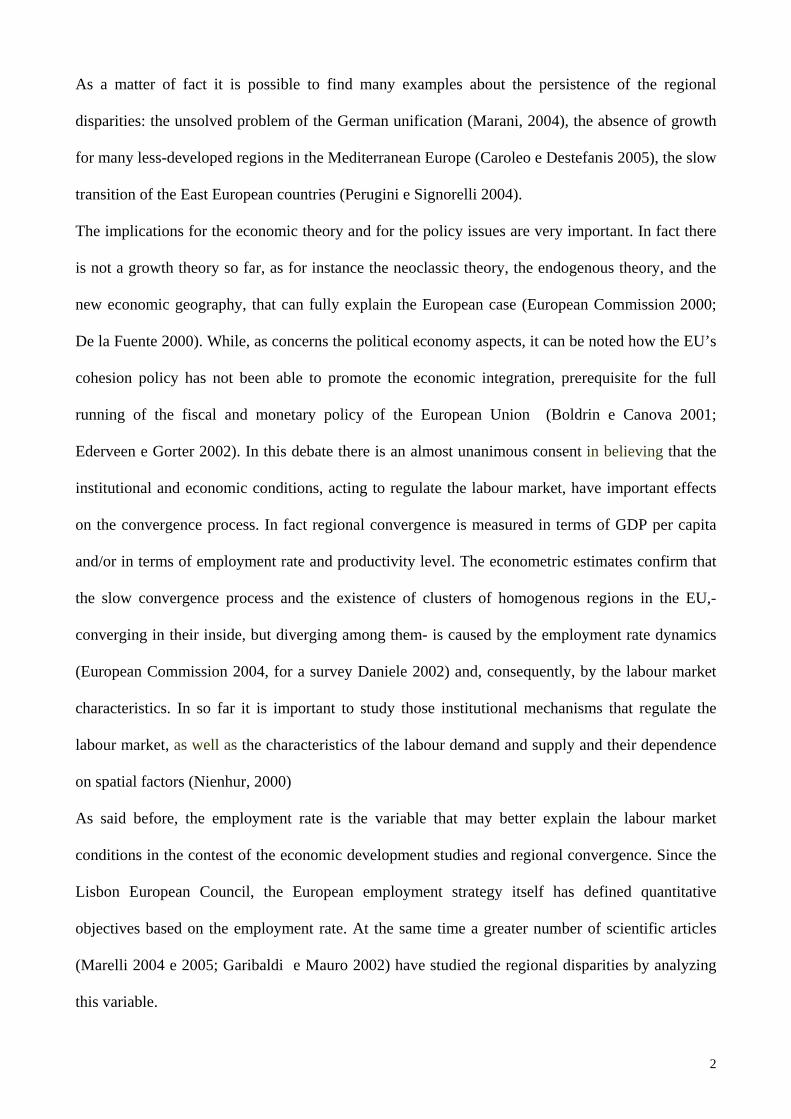
The most important stylized fact in the European Union is shown in the graphs 1 and 2, where are

represented the index number of the mean, mean square error, and coefficient of variation of the

employment rate (graph 1), and of the unemployment rate (graph 2) relating to 130 European

regions for the period 1991 to 2000. We can observe two important stylized facts: the first one is

that in the Nineties the unemployment rate has shown a higher cycle than the employment rate, and

the other one is that the variability of the unemployment rate at regional level has been higher than

the employment rate.

4

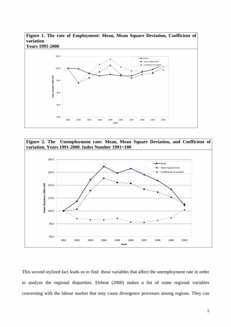
Figure 1. The rate of Employment: Mean, Mean Square Deviation, Coefficient of variation Years 1991-2000

80,0

85,0

90,0

95,0

100,0

105,0

1991 1992 1993 1994 1995 1996 1997 1998 1999 2000Anni

Inde

x N

umbe

r 199

1=10

0

Mean

Mean Square Error

Coefficient of variation

Figure 2. The Unemployment rate: Mean, Mean Square Deviation, and Coefficient of variation. Years 1991-2000. Index Number 1991=100

80,0

90,0

100,0

110,0

120,0

130,0

140,0

1991 1992 1993 1994 1995 1996 1997 1998 1999 2000Anni

Inde

x N

umbe

rs 1

991=

100

Mean

Mean Square Error

Coefficiente of variation

This second stylized fact leads us to find those variables that affect the unemployment rate in order

to analyze the regional disparities. Elrhost (2000) makes a list of some regional variables

concerning with the labour market that may cause divergence processes among regions. They can

5

be synthesized in the different endowment in the product factors and in the “fundamentals”; in the

different local labour market structure (Genre e Gòmez-Salvador, 2002) –demographic growth,

population age-structure, migration and commuting (Greenway, Upward e Wright, 2002); in the

employment levels; in the productive structure (Marelli, 2003; Paci e Pigliaru, 1999; Paci, Pigliaru e

Pugno, 2002); in the demographic density and urbanization (Taylor e Bradley 1997); in the

economic and social barriers; in the human capital; in the institutional structure regulating the good

markets and the labour market, and also the wages composition (Pench e Sestito e Frontini,1999;

Hyclack e Johnes 1987).

Without expecting to be exhaustive, we want to test some of the theses above mentioned. To this

end we want to estimate the relationship between the unemployment rate, measured at the regional

level, and a set of variable that includes some institutional indicators and the most important

regional economic characteristics.

2. The set of the independent variables.

The set of the independent variables used in our analysis may be classified into three groups: (a)

productive structure and labour market indicators, (b) institutional indicators and (c) variables of the

economic performance.

Indicators of the productive structure and labour market

We begin to estimate a proxy of the labour market and productive structures of the regions. To this

end, we calculate two indicators by applying a dynamic multivariate factorial analysis. This method

is very useful to study multidimensional phenomena like the regional disparities. In fact the regions

(cases) may be analyzed on the base of a set of indicators (variables) that change over the years

(time).

6

We choose (Amendola, Caroleo, Coppola 2004) to apply the STATIS (Structuration des Tables A

Trois Indeces de la Statistique) method (Escoufier 1985 e 1987). This is a dynamic multivariate

method that is able to cluster the regions for several years on the base of a set of variables including

indicators of labour market and income, variables of the composition of the population and of the

structure of the productive sector. In this way it is possible to study the interaction chances between

the labour market structure and the economic growth over time. In this contest, it is also possible to

analyze the dynamics of the regions.

The variables used for this analysis are listed in Table 3.2. They are taken from the Eurostat REGIO

database and the European regions database of Cambridge Econometrics Ltd. and they are, as said,

indicators characteristic of the labour market and the production system (Wishlade and Yuill, 1997).

The labour demand is measured by the unemployment rate on the total working-age population

(TOT), while the labour supply is measured by the labour-force participation rate (TAT). The

percentage of the long-term unemployed (ULR) is used as a proxy for the structural gap between

labour demand and supply. The percentage of part-time employment (PTT) is used as a measure of

the flexibility of the regional labour market.

The production system is represented by four variables corresponding to the percentages of

employed persons in agriculture (AGR), industry (IND), traditional services – commerce, hotels

and non-market services (GHM) – and advanced services – transport, financial services and others

(IJA). The other variables considered are population density (DEN), as a proxy for the gravitational

force of a region, and per capita income (PPS), which is the indicator most frequently used to

represent regional disparities.

7

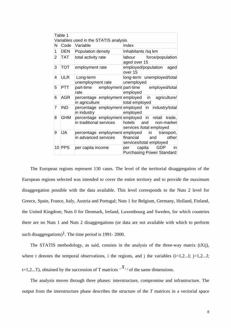
Table 1 Variables used in the STATIS analysis N Code Variable Index 1 DEN Population density Inhabitants /sq km 2 TAT total activity rate labour force/population

aged over 15 3 TOT employment rate employed/population aged

over 15 4 ULR Long-term

unemployment rate long-term unemployed/total unemployed

5 PTT part-time employment rate

part-time employed/total employed

6 AGR percentage employment in agriculture

employed in agriculture/ total employed

7 IND percentage employment in industry

employed in industry/total employed

8 GHM percentage employment in traditional services

employed in retail trade, hotels and non-market services /total employed

9 IJA percentage employment in advanced services

employed in transport, financial and other services/total employed

10 PPS per capita income per capita GDP in Purchasing Power Standard

The European regions represent 130 cases. The level of the territorial disaggregation of the

European regions selected was intended to cover the entire territory and to provide the maximum

disaggregation possible with the data available. This level corresponds to the Nuts 2 level for

Greece, Spain, France, Italy, Austria and Portugal; Nuts 1 for Belgium, Germany, Holland, Finland,

the United Kingdom; Nuts 0 for Denmark, Ireland, Luxembourg and Sweden, for which countries

there are no Nuts 1 and Nuts 2 disaggregations (or data are not available with which to perform

such disaggregations)1. The time period is 1991- 2000.

The STATIS methodology, as said, consists in the analysis of the three-way matrix (tXij),

where t denotes the temporal observations, i the regions, and j the variables (i=1,2...I; j=1,2...J;

t=1,2...T), obtained by the succession of T matrices of the same dimensions. jit X ,

The analysis moves through three phases: interstructure, compromise and infrastructure. The

output from the interstructure phase describes the structure of the T matrices in a vectorial space

8

smaller than T. This is reduced to two dimensions but still maintains a good similarity to the initial

representation. The compromise phase consists in the estimation of a synthesis matrix which yields

a representation, in the two-dimensional space identified, of the characteristic indicators and of the

average positions of the regions in the time-span analysed (1991-2000). The result of this

intrastructure phase is a representation of the trajectories followed by the individual regions in the

same period of time.

Table 2 Eigenvalues and inertia percentages of the factorial axes Axis Eigenvalue Variance explained Cumulated variance

explained 1 3.75547 36.76 36.76 2 1.99895 19.56 56.32 3 1.18853 11.63 67.95

In order to evaluate the goodness of the factorial representation yielded by construction of the

compromise matrix, Table 2 shows the first three highest eigenvalues and the percentage of the total

variance explained by the first three factorial axes.

To be noted first is that 36.8% of the variance is explained by the first factor, and 19.6% by the

second, for a total of 56.3% of the variance expressed by the set of all the variables. In other words,

the first factor alone explains more than one-third of the total variability, while the first three factors

jointly explain almost 68%. Consequently, the reduction of the phenomenon’s variability, obtained

by representing it in a two-dimensional space, is a meaningful synthesis of the information

considered.

In order to interpret the two figures, we may refer to Table 2, which shows that minimum and

maximum period values of the correlations between the variables and the factorial axes. It will be

seen that the variables most closely correlated with the first factor are, on the one hand, the

employment rate (TOT), the activity rate (TAT), the percentage of part-time employment (PTT),

per capita income (PPS), and the percentage of employment in advanced services; and on the other

(positive quadrant), the percentage of long-term unemployment (ULR), and the percentage of

1 The complete list of the 130 regions is given in the Appendix.

9

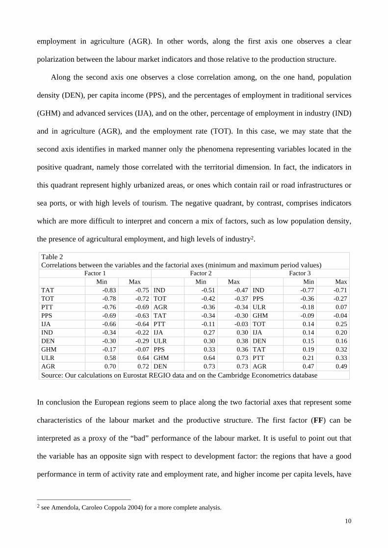
employment in agriculture (AGR). In other words, along the first axis one observes a clear

polarization between the labour market indicators and those relative to the production structure.

Along the second axis one observes a close correlation among, on the one hand, population

density (DEN), per capita income (PPS), and the percentages of employment in traditional services

(GHM) and advanced services (IJA), and on the other, percentage of employment in industry (IND)

and in agriculture (AGR), and the employment rate (TOT). In this case, we may state that the

second axis identifies in marked manner only the phenomena representing variables located in the

positive quadrant, namely those correlated with the territorial dimension. In fact, the indicators in

this quadrant represent highly urbanized areas, or ones which contain rail or road infrastructures or

sea ports, or with high levels of tourism. The negative quadrant, by contrast, comprises indicators

which are more difficult to interpret and concern a mix of factors, such as low population density,

the presence of agricultural employment, and high levels of industry2.

Table 2 Correlations between the variables and the factorial axes (minimum and maximum period values)

Factor 1 Factor 2 Factor 3 Min Max Min Max Min Max

TAT -0.83 -0.75 IND -0.51 -0.47 IND -0.77 -0.71TOT -0.78 -0.72 TOT -0.42 -0.37 PPS -0.36 -0.27PTT -0.76 -0.69 AGR -0.36 -0.34 ULR -0.18 0.07PPS -0.69 -0.63 TAT -0.34 -0.30 GHM -0.09 -0.04IJA -0.66 -0.64 PTT -0.11 -0.03 TOT 0.14 0.25IND -0.34 -0.22 IJA 0.27 0.30 IJA 0.14 0.20DEN -0.30 -0.29 ULR 0.30 0.38 DEN 0.15 0.16GHM -0.17 -0.07 PPS 0.33 0.36 TAT 0.19 0.32ULR 0.58 0.64 GHM 0.64 0.73 PTT 0.21 0.33AGR 0.70 0.72 DEN 0.73 0.73 AGR 0.47 0.49Source: Our calculations on Eurostat REGIO data and on the Cambridge Econometrics database

In conclusion the European regions seem to place along the two factorial axes that represent some

characteristics of the labour market and the productive structure. The first factor (FF) can be

interpreted as a proxy of the “bad” performance of the labour market. It is useful to point out that

the variable has an opposite sign with respect to development factor: the regions that have a good

performance in term of activity rate and employment rate, and higher income per capita levels, have

2 see Amendola, Caroleo Coppola 2004) for a more complete analysis.

10

negative value of this factor. On the contrary those regions that have low activity and employment

rates and a high percentage employed in agriculture.

The second factor (SF) may be interpreted as a factor that is positive correlated with the

urbanization and a high developed tertiary sector.

Institutional Variables

If the first factor, obtained by STATIS, may be interpreted as the level of efficiency and of

flexibility of the labour market, a further indicator of the rigidity/flexibility of the labour market

may be found in the degree of decentralization of those institutions regulating the labour market

and, particularly, the level of wage bargaining centralization (Calmfors, 1993; Calmfors e Driffil,

1988).

For a long time, the “European model” has been characterized by wage bargaining strictly related

with the industrial relations, or rather, with an institutional framework aimed at the employment

protection, centralized, universalistic and egalitarian. Nevertheless in the last years many things

have changed. A new trend, regarding the need to decentralize the labour market policies at a sub

national level (i.e. regional), has been developed according to the thesis that considers the

participation in bargaining by the local institution as a way to reach a higher level of regional

cohesion in the EU (Buti, Pench e Sestito, 1998; Soltwedel, Dohse e Kreige-Boden, 1999).

Usually the debate on bargaining has been focused on the centralized or decentralized wage

bargaining as a vertical kind of bargaining (i.e from national to firm level) (Freeman e Gibbson

1993). The firm-level bargaining is considered by the OECD (OECD,1999) the only one that may

reduce the regional disparities since it binds the bargained wage to the different local labour market

conditions and to the different regional labour productivity (for the Italian case see Antonelli e

Paganetto (1999), Biagioli, Caroleo and Destefanis (1999) and, more recently, Dell’Aringa (2005)).

There are many possible objections to this approach. As a matter of fact it has been pointed out that

there is a variety of bargaining modalities (bargaining at regional level or by skills) and, on the

other side, that there is a coordination problem (Amendola, Caroleo e Garofalo, 1997).

11

If we consider these two aspects together, it is possible to show that the economic performance can

be improved both by a centralized and by a decentralized bargaining.

It may be useful to underline that the bargaining decentralization cannot be separated from the

industrial relation assets. This crucial aspect is important in order to better understand the reasons of

a bargaining reform aimed at decentralizing the wage bargaining, but that at the same time takes

into account the different institutional framework and the coordination issues

In other words the industrial relations concern that security system built up to protect the

employment like the security (i) against the risk of the future unemployment and the job

precariousness, (ii) against the barriers to the Human capital development, (iii) against the

restriction on the right to work and against the (iv) low representativeness of the workers.

These industrial relations should be adjusted according to the characteristics of the local labour

markets. In fact, the labour market policies are aimed at implementing active policies that are

appropriate to the different local labour market characteristics, with also different applicatory

approaches that involve several actors and procedures.

A decentralized industrial relations system need to go beyond a mere decentralization of the

administrative bureaucratic system. It should involve the most important local actors, implement

shared actions with shared responsibilities (Regini, 2002, Arrighetti e Seravalli, 1999).

This is the only way to obtain a kind of employment growth that is both quantitative and qualitative,

or, in other words, to make more flexible the labour market without loosing the necessary securities.

For this reason the new approach of decentralization of the industrial relations has been interpreted

as a tendency to the local and territorial “negotiations “ that assumes the form of a pact among the

interested social parts.

For our analysis it would be useful to find, as a proxy of the institutional decentralization of the

labour market, a variable related to the level of decentralized bargaining and to the degree of the

regional industrial relations system. Unfortunately, homogeneous data at the European level are not

available, therefore we can only use the traditional indicator of the bargaining centralization

12

(CENTR) that combines the levels of wage bargaining centralization with the wage coordination

among the most important trade unions (Checchi e Lucifora 2002; Boeri, Brugiavini e Calmfors

2002).

The underlying hypothesis is that if the trade union bargains the wage at the level of the single firm

it will better take into account the firm productivity level, that surely is affected by the local

economic conditions.

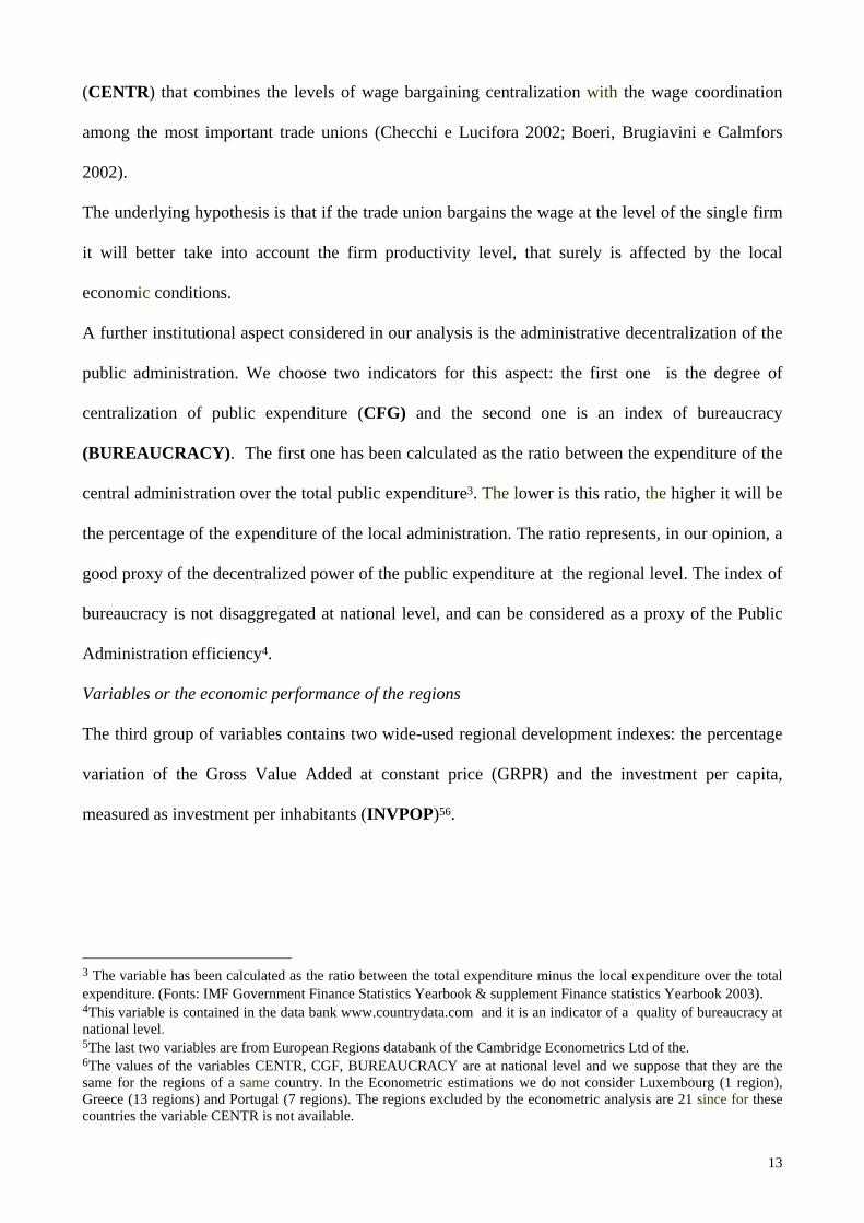
A further institutional aspect considered in our analysis is the administrative decentralization of the

public administration. We choose two indicators for this aspect: the first one is the degree of

centralization of public expenditure (CFG) and the second one is an index of bureaucracy

(BUREAUCRACY). The first one has been calculated as the ratio between the expenditure of the

central administration over the total public expenditure3. The lower is this ratio, the higher it will be

the percentage of the expenditure of the local administration. The ratio represents, in our opinion, a

good proxy of the decentralized power of the public expenditure at the regional level. The index of

bureaucracy is not disaggregated at national level, and can be considered as a proxy of the Public

Administration efficiency4.

Variables or the economic performance of the regions

The third group of variables contains two wide-used regional development indexes: the percentage

variation of the Gross Value Added at constant price (GRPR) and the investment per capita,

measured as investment per inhabitants (INVPOP)56.

3 The variable has been calculated as the ratio between the total expenditure minus the local expenditure over the total expenditure. (Fonts: IMF Government Finance Statistics Yearbook & supplement Finance statistics Yearbook 2003). 4This variable is contained in the data bank www.countrydata.com and it is an indicator of a quality of bureaucracy at national level. 5The last two variables are from European Regions databank of the Cambridge Econometrics Ltd of the. 6The values of the variables CENTR, CGF, BUREAUCRACY are at national level and we suppose that they are the same for the regions of a same country. In the Econometric estimations we do not consider Luxembourg (1 region), Greece (13 regions) and Portugal (7 regions). The regions excluded by the econometric analysis are 21 since for these countries the variable CENTR is not available.

13

List of the Dependent Variables Acronym Variables CONS Constant FF Index factor of the labour market’s performance

(the variable has an opposite sign related to development’s index) SF Index factor of tertiary/urbanization CENTR bargaining centralization index CGF level of public expenditure centralization BUREAUCRACY Bureaucracy’ index GDPG GDP annual growth at constant price INVPOP investment/population

3. The Estimation Method: The Panel Data analysis

Our dataset is a Panel Data where the cases are the regions e the time units are the years from 1991

to 2000. For this reasons we apply the Panel data econometric methods to study the relationship

between the unemployment rate and the set of the independent variables

The model may be written as

ititit zxy εαβα +++= ''0 [1]

where , . is the constant, ni ,.......1= Tt .,.........1= 0a β is the vector of coefficients, contains K

regressors and the matrix , is a set of not observable variables that captures the specific effects

related to the characteristics of the individuals that are, in our study, 109 European regions

itx

itz

7. itε is

the error term.

The variables in are not observed and may be correlated or not correlated with the regressors. In

the first case in the model [1] the intercept is group specific and it is constant over the time. This is

the Fixed Effects model and may be written as:

itz

itiitit xay εαβ +++= '0 [2]

7 As we say before, the variable CENTR is not available for some nations.

14

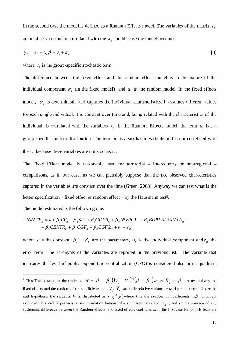
In the second case the model is defined as a Random Effects model. The variables of the matrix

are unobservable and uncorrelated with the . In this case the model becomes

itz

itx

itiitit uxy εβα +++= '0 [3]

where is the group-specific stochastic term. iu

The difference between the fixed effect and the random effect model is in the nature of the

individual component iα (in the fixed model) and in the random model. In the fixed effects

model,

iu

iα is deterministic and captures the individual characteristics. It assumes different values

for each single individual, it is constant over time and, being related with the characteristics of the

individual, is correlated with the variables . In the Random Effects model, the term has a

group specific random distribution. The term is a stochastic variable and is not correlated with

the , because these variables are not stochastic.

ix iu

iu

ix

The Fixed Effect model is reasonably used for territorial – intercountry or interregional –

comparisons, as in our case, as we can plausibly suppose that the not observed characteristics

captured in the variables are constant over the time (Green, 2003). Anyway we can test what is the

better specification – fixed effect or random effect – by the Hausmann test8.

The model estimated is the following one:

itiititit

itititititit

CGFCGFCENTRYBUREAUCRACINVPOPGDPRSFFFaUNRATE

ενββββββββ

+++++++++++=

2 876

54321

where is the constant, a 81......ββ are the parameters, iυ is the individual component and itε the

error term. The acronyms of the variables are reported in the previous list. The variable that

measures the level of public expenditure centralization (CFG) is considered also in its quadratic

8 This Test is based on the statistics ( ) ( ) ( )rfrfrf VVW ββββ −−−= −1' where fβ and rβ are respectively the

fixed effects and the random effect coefficients and , . are their relative variance-covariance matrixes. Under the

null hypothesis the statistics W is distributed as a fV rV( )k2χ where k is the number of coefficients inβ , intercept

excluded. The null hypothesis in no correlation between the stochastic term and , and so the absence of any systematic difference between the Random effects and fixed effects coefficients. In the first case Random Effects are

itx

15

form (CFG2) in order to test the hypothesis of a quadratic relationship of this variable with the

unemployment rate and, consequently, the existence of an optimal dimension in the degree of

centralization of public expenditure.

Results

The Table 4 contains the results. In the third and fourth columns are reported respectively the

Random Effects and the Fixed Effects estimates. For sake of completeness this table includes also

the OLS estimation (column 1) and the Random effect model results obtained by the Maximum

Likelihood Estimation (columns 1).

The signs of the coefficients, obtained by the four estimation methods, are always the same. The

Hausmann test does not accept the null hypothesis of absence of correlation between the dependent

variables and the error terms. This is the fundamental hypothesis of the Random effects model, and

being not accepted, we can conclude that the Fixed Effect model is the well specified model.

The result confirms the theories of the previous paragraphs. Particularly in the Fixed Effect Model

the coefficients are all statistically significative and they have the expected sign. Only the variable

GDPR – the annual growth rate of the gross value added per capita- is significative only at the 8%.

The dependent variables are expressed in different measures. Accordingly, in order to compare the

dimension of their effects on the unemployment rate, we calculate the standard coefficients9 of the

variables and the elasticity to their mean value (tab. 5) 10.

better than Fixed Effects because the Random Effects are more efficient. In the opposite case the Fixed Effects are consistent.

9 A standard coefficient is equal toy

xx

sx s

si

iiββ = where xβ is the parameter of the variable , and are

respectively the standard deviations of the variable and y. It may be useful to make an example to better understand the meaning of the standard coefficients. The standard coefficient of the variable SF (Table 5) is 0.6; this means that a unit standard deviation of SF causes a standard deviation of the unemployment rate equal to 0.6.

ix xs ys

ix

10 The elasticity of an independent variable to its mean value is YX

YX

YXE xx ∂

∂== β . It may be useful to point out

that the standard coefficients, even if they are more difficult to analyse, are constant for all the values of the relative

16

Summary and Conclusions

The results obtained seem to confirm our initial thesis: the unemployment rate is correlated with

the decentralization level of the wage bargaining, with the institutional efficiency of the regions,

and also with the bureaucracy level, even if the impact of this variable on the unemployment rate is

small.

The centralization level of the public expenditure has a quadratic relationship with the

unemployment rate. This means that the unemployment level grows together with the public

expenditure centralization degree, but in a less than proportional way, until a value of the

centralization ratio equal to 75%. After that value the unemployment decreases. Nevertheless, we

need to be cautious in interpreting this result since the sign of the variables CGF and CFG2 is

opposite in the OLS Method.

Also the economic performance of the regions – measured by the GDP growth and the investment

per capita (INVPOP) –has a negative impact on the unemployment rate. The second variable has a

standard coefficient that is double compared with the first one.

We find also interesting the value of the two structural factors coefficients. In fact, as it can be

easily supposed, the unemployment rate is negatively correlated with the good performance of the

regional labour market (high activity and employment rate, high share of employment in the

industrial and in the advanced services sector) measured by the first factor (FF).

Even if it is more difficult to explain the positive relationship between the unemployment rate and

the second factor that is related to the high share of the services and high demographic density. In

this case the results seem to confirm the empirical evidence - reported also in the third Progress

Report on Economic and Social Cohesion in the EU – that the “cities act as centres of employment

for a widely-drawn population, with one in every three jobs being taken by someone commuting into

the city” (Commission of the European Communities, Third Progress Report on Cohesion, page

22). For this reason the unemployment and social problems in the European Union assume a higher

independent variable. On the contrary, in our estimations the elasticity of a dependent variable is not constant because the model is linear.

17

relevance in Urban centres as well as in the tertiary process that nowadays characterizes the EU

economic development.

.

18

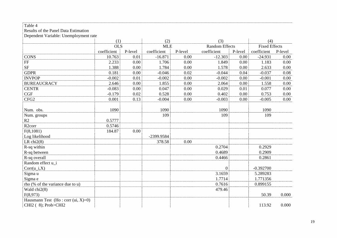
Table 4 Results of the Panel Data Estimation Dependent Variable: Unemployment rate (1) (2) (3) (4) OLS MLE Random Effects Fixed Effects

coefficient P-level coefficient P-level coefficient P-level coefficient P-levelCONS 10.763 0.01 -16.871 0.00 -12.303 0.00 -24.931 0.00FF 2.233 0.00 1.706 0.00 1.849 0.00 1.183 0.00SF 1.388 0.00 1.784 0.00 1.578 0.00 2.633 0.00GDPR 0.181 0.00 -0.046 0.02 -0.044 0.04 -0.037 0.08INVPOP -0.002 0.01 -0.002 0.00 -0.002 0.00 -0.001 0.00BUREAUCRACY 2.646 0.00 1.855 0.00 2.064 0.00 1.558 0.00CENTR -0.083 0.00 0.047 0.00 0.029 0.01 0.077 0.00CGF -0.179 0.02 0.528 0.00 0.402 0.00 0.753 0.00CFG2 0.001 0.13 -0.004 0.00 -0.003 0.00 -0.005 0.00 Num. obs. 1090 1090 1090 1090 Num. groups 109 109 109 R2 0.5777 R2corr 0.5746 F(8,1081) 184.87 0.00Log likelihood -2399.9584 LR chi2(8) 378.58 0.00 R-sq within 0.2704 0.2929 R-sq between 0.4689 0.2909 R-sq overall 0.4466 0.2861 Random effect u_i Corr(u_i,X) 0 -0.392700Sigma u 3.1659 5.289283 Sigma e 1.7714 1.771356 rho (% of the variance due to u) 0.7616 0.899155 Wald chi2(8) 479.46 F(8,973) 50.39 0.000Hausmann Test (Ho : corr (ui, X)=0) CHI2 ( 8); Prob>CHI2 113.92 0.000

19

Table 5 Mean, Standard deviation, coefficients, (fixed effect), standard coefficients, elasticity at mean value

Variable Mean s.d . parameter c s el UNEMPLOYMENT RATE 10.885 6.064 CONSTANT -24.931 FF -0.300 1.766 1.183 0.344 -0.033 SF 0.171 1.384 2.633 0.601 0.041 GDPR 2.029 3.260 -0.037 -0.020 -0.007 INVPOP 50.239 178.694 -0.001 -0.044 -0.007 BUREAUCRACY 3.974 0.143 1.558 0.037 0.569 CENTR 25.747 16.247 0.077 0.207 0.183 CGF 73.082 8.256 0.753CGF2 5409.132 991.429 -0.005 0.199 0.289

20

APPENDIX The 130 European regions. sigla Regioni sigla Regions Belgium – NUTS 1 – Regions be1 Région Bruxelles-

capitale/Brussels hoofdstad gewest

be2 Vlaams Gewest

be3 Région Wallonne dk Denmark – NUTS 0 – Nation Federal Republic of Germany (including ex-GDR from 1991)

- NUTS 1 – Lander de1 Baden-Württemberg de2 Bayern de3 Berlin de4 Brandenburg de5 Bremen de6 Hamburg de7 Hessen de8 Mecklenburg-Vorpommern de9 Niedersachsen dea Nordrhein-Westfalen deb Rheinland-Pfalz dec Saarland ded Sachsen dee Sachsen-Anhalt def Schleswig-Holstein deg Thüringen Greece – NUTS 2 – Development regions gr11 Anatoliki Makedonia, Thraki gr12 Kentriki Makedonia gr13 Dytiki Makedonia gr14 Thessalia gr21 Ipeiros gr22 Ionia Nisia gr23 Dytiki Ellada gr24 Sterea Ellada gr25 Peloponnisos gr3 Attiki gr41 Voreio Aigaio gr42 Notio Aigaio gr43 Kriti Spain – NUTS 2 – Comunidades autonomas es11 Galicia es12 Principado de Asturias es13 Cantabria es21 Pais Vasco es22 Comunidad Foral de Navarra es23 La Rioja es24 Aragón es3 Comunidad de Madrid es41 Castilla y León es42 Castilla-la Mancha es43 Extremadura es51 Cataluña es52 Comunidad Valenciana es53 Baleares es61 Andalucia es62 Murcia es63 Ceuta y Melilla (ES) es7 Canarias (ES) France – NUTS 2 – Régions Fr1 Île de France fr21 Champagne-Ardenne Fr22 Picardie fr23 Haute-Normandie Fr24 Centre fr25 Basse-Normandie Fr26 Bourgogne fr3 Nord - Pas-de-Calais Fr41 Lorraine fr42 Alsace Fr43 Franche-Comté fr51 Pays de la Loire Fr52 Bretagne fr53 Poitou-Charentes Fr61 Aquitaine fr62 Midi-Pyrénées Fr63 Limousin fr71 Rhône-Alpes Fr72 Auvergne fr81 Languedoc-Roussillon Fr82 Provence-Alpes-Côte d'Azur fr83 Corse Ie Ireland – NUTS 0 – Nations Italy – NUTS 2 – Regioni It11 Piemonte it12 Valle d'Aosta It13 Liguria it2 Lombardia It31 Trentino-Alto Adige it32 Veneto

21

It33 Friuli-Venezia Giulia it4 Emilia-Romagna It51 Toscana it52 Umbria It53 Marche it6 Lazio It71 Abruzzo it72 Molise It8 Campania it91 Puglia It92 Basilicata it93 Calabria Ita Sicilia itb Sardegna Lu Luxembourg Netherlands – NUTS 2 – Provincies nl1 Noord-Nederland nl2 Oost-Nederland nl3 West-Nederland nl4 Zuid-Nederland Austria – NUTS 2 – Bundesländer at11 Burgenland at12 Niederösterreich at13 Wien at21 Kärnten at22 Steiermark at31 Oberösterreich at32 Salzburg at33 Tirol at34 Vorarlberg Portugal - NUTS 2 groupings pt11 Norte pt12 Centro (P) pt13 Lisboa e Vale do Tejo pt14 Alentejo pt15 Algarve pt2 Açores (PT) pt3 Madeira (PT) Finland- NUTS 1 – Manner-Suomi/Ahvenanmaa Fi1 Manner-Suomi fi2 Åland se Sweden- NUTS 0 – Nation United Kingdom –NUTS 1 – Nation ukc North East ukd North West (including Merseyside) uke Yorkshire and The Humber ukf East Midlands ukg West Midlands ukh Eastern uki London ukj South East ukk South West ukl Wales ukm Scotland ukn Northern Ireland

22

References

Amendola A., Caroleo F.E., Coppola G., (2005) Regional Disparities in Europe in Caroleo and Destefanis (eds), (2005) Regions, Europe and the Labour Market. Recent Problems and Developments, Physica Verlag, Heidelberg.

Amendola A., Caroleo F.E., Garofalo M. (1997), “Labour Market and Decentralized Decision Making: an Institutional Approach”, Labour, (11), 3, 497-516.

Antonelli G., Paganetto L. (a cura di) (1999), Disoccupazione e basso livello di attività, il Mulino, Bologna.

Arrighetti A., Seravalli G. (a cura di) (1999), Istituzioni intermedie e sviluppo locale, Donzelli, Roma

Biagioli M., Caroleo F. E., Destefanis S. (eds.) (1999), “Introduzione” a Struttura della contrattazione, differenziali salariali e occupazione in ambiti regionali, ESI, Napoli.

Blanchard O., Wolfers J. (2000), “The Role of Shocks and Institutions in the Rise of European Unemployment: The Aggregate Evidence”, Economic Journal, March. C1-C33.

Bodo G., Sestito P. (1991), Le vie dello sviluppo, il Mulino, Bologna. Boeri T., Brugiavini A., Calmfors L. (2002) Il ruolo del sindacato in Europa, Università Bocconi

Editore, Milano. Boldrin M. and Canova F. (2001), “Inequality and Convergence in Europe’s Regions:

Reconsidering European Regional Policies”, Economic Policy, April 2001. Buti M., Pench L. R., Sestito P. (1998), “European Unemployment: Contending Theories and

Institutional Complexities” , DGII, Working paper n. 81, Brussels. Perugini C., Signorelli M., (2004)” Employment Performance and Convergence in the European

Countries and Regions”, The European Journal of Comparative Economics, vol. 1, n. 2, 2004, pp. 243-278) .

Calmfors L. (1993), “Centralization of Wage Bargaining and Macroeconomic Performance: a Survey”, OECD Economic Studies, n. 2, 161-191.

Calmfors L., Driffill J. (1988), “Bargaining Structure, Corporatism and Macroeconomic Performance”, Economic Policy, 6, 15-61.

Caroleo F.E. (2000), “Le politiche per l'occupazione in Europa: Una tassonomia istituzionale”, Studi Economici, n. 71, 2, 115-152.

Caroleo F. E., Destefanis S. (eds) (2005) Regions, Europe and the Labour Market. Recent Problems and Developments, Physica Verlag, Heidelberg.

Checchi D., Lucifora C., (2002), “Unions and labour market institutions in Europe”, Economic Policy 2002, 362-408

Daniele V. (2002), “Integrazione economica e monetaria e divari regionali nell’Unione Europea” Rivista economica del Mezzogiorno, 3:513–550.

De la Fuente A (2000), “Convergence across countries and regions: theory and empirics”, European Investment Bank Papers 2.

Dell’Aringa C. (2005), “Industrial Relations and Macroeconomic Performance” , Paper presentato alla Conferenza Internazionale su “Social Pacts, Employment and Growth: A Reappraisal of Ezio Tarantelli’s Thought”, Roma.

Ederveen S., Gorter J. (2002), “Does European Cohesion Policy Reduce Regional Disparities? An empirical Analysis”, CPB Netherland Bureau for Economic Policy Analysis, CPB Discussion Paper, n. 15.

Elhorst JP. (2000), “The mystery of regional unemployment differentials: a survey of theoretical and empirical explanations” Research Report 00C06, University of Groningen, Research Institute SOM-Theme C: Coordination and Growth in Economics.

Escoufier Y. (1985), “Statistique et analyse des données”, Bulletin des Statisticiens Universitaires 10.

23

Escoufier Y. (1987), Three-mode data analysis: the Statis method. in Methods for multidimensional data analysis, European Courses in Advanced Statistics.

European Commission (2000), Real convergence and catching up in the EU, in the EU economy: 2000 Review, European Commission, Luxembourg.

European Commission (2004), “A New Partnership for Cohesion: Convergence, Competitiveness, Cooperation”, Third Report on Economic and Social Cohesion, Brussels.

European Commission (2005), Third Progress Report on Cohesion, Brussels Freeman R. B., Gibbson R. (1993), “Getting Together and Breaking Apart: the Decline of

Centralized Collective Bargaining”, NBER Working Paper, n. 4464, Cambridge, Mass. Garibaldi P. and Mauro P., (2002), "Anatomy of Employment Growth", Economic Policy, Vol. 17,

pp. 67-113. Genre V, Gòmez-Salvador R., (2002), “Labour force developments in the Euro area since the

1980s”. ECB Occasional Paper Series 4. Greenway D, Upward R., Wright P. (2002), “Structural adjustment and the sectoral and

geographical mobility of labour. Leverhulme Centre for Research on Globalisation and Economic Policy” Working Paper n.3, University of Nottingham.

Green W. H., (2003), Econometric Analysis, Fifth edition, Prentice Hall International Edition Hausman J. (1978), “Specification Tests in Econometrics”, Econometrica, 46, 1978, pp.1251-1271 Hyclak T, Johnes G., (1987), “On the determinants of full employment unemployment rates in

local labour markets”, Applied Economics 19:615–645. International Monetary Found Government Finance Statistics Yearbook & Supplement Finance

statistics Yearbook, 2003 Layard R., Nickell S., Jackman R., Unemployment. Macroeconomic Performance and the Labour

Market, Oxford University Press, Londra, 1991. Marani U. (a cura di) (2005), L’economia della Germani Unificata: uno sguardo interessato dal

Mezzogiorno d’Italia, Donzelli Editore, Roma. Marelli E. (2004a), “Evolution of Employment Structures and Regional Specialisation in the EU”,

Economic Systems, 28, 35-59 Marelli E. (2005), ‘Regional Employment Dynamics in the EU: Structural Outlook, Co-movements,

Clusters and Common Shocks’, in Caroleo F.E., Destefanis (Eds): Regions, Europe and the Labour Market: Recent Problems and Developments, Heidelberg, Physica-Verlag

Nickell S. (1997), “Unemployment and Labor Market Rigidities: Europe versus North America”, Journal of Economic Perspectives, vol. 11, n. 3, 1997, 55-74.

Nickell S., Layard R., (1999), “Labour Market Institutions and Economic Performance”, in Ashenfelter, Card (1999). Ashenfelter O., Card D. (a cura di), Handbook of Labor Economics, North Holland.

Niebuhr A., (2002), Spatial dependence of regional unemployment in the European Union. HWWA Discussion Paper 186.

Oecd, (1999), Employment Outlook, Paris, . Paci R, Pigliaru F, Pugno M., (2002), Le disparità nella crescita economica e nella disoccupazione

tra le regioni europee: una prospettiva settoriale. In: Farina F, Tamborini R (eds), Da nazioni a regioni: mutamenti istituzionali e strutturali dopo l’Unione Monetaria Europea, Il Mulino, Bologna.

Pench LR, Sestito P, Frontini E., (1999), “Some unpleasant arithmetics of regional unemployment in the EU, are there any lessons for EMU?”. European Union DG XII, Brussel.

Paci R, and Pigliaru F., (1999), European regional growth: do sectors matter? In: Adams J, Pigliaru F. (eds), Economic growth and change, national and regional patterns of convergence and divergence, Edward Elgar, Celthenam.

Soltwedel R., Dohse D., Krieger-Boden C. (1999), “EMU Challanges European Labor Markets”, IMF Working Paper n. 99/131, Washinghton D.C., 1999.

Taylor J, Bradley S., (1997), “Unemployment in Europe: a comparative analysis of regional disparities in Germany, Italy and the UK”. Kyklos, 50(2):221–245.

24