the impact of the interest rate level on bank ... · the impact of the interest rate level on bank...
TRANSCRIPT

the impact of the iNterest rate level oN baNk profitability
aNd balaNce sheet structure
carlos pérez montes and alejandro ferrer pérez (*)
We would like to express our gratitude to the corresponding editor of the Review of Financial Stability and an anonymous referee. We also appreciate the help and comments of Nadia lavín san segundo and the comments received from Jesús saurina and carlos trucharte.
this article is the exclusive responsibility of the authors and does not necessarily reflect the opinion of the banco de españa or the eurosystem.
(*) banco de españa, dg financial stability, regulation and resolution.

BANCO DE ESPAÑA 125 REVISTA DE ESTABILIDAD FINANCIERA, NÚM. 35
ThE IMPACT oF ThE INTEREST RATE LEVEL oN BANk PRoFITABILITy
AND BALANCE ShEET STRUCTURE
We study the sensitivity of bank profits and balance sheet structure to changes in the level
of interest rates in spain during the 2000-2016 period. autoregressive distributed lag
(ardl) models with controls for the business cycle and interest rate levels are estimated
for the time series of key asset and liability categories (credit, financial securities, time
deposits, etc.) and profit components (returns on asset and liabilities, provision charges,
etc.). We find a non-linear relation between interest rates and net interest income, which is
positive at low interest rate levels. this relation is driven by the effect of interest rates on
asset and liability returns, and also on credit growth, and on the bank mix of credit,
deposits and financial securities. broader profit measures also present a non-linear relation
with interest rates, which can be negative even for low interest rate levels if provisioning
charges are high enough.
the observation of low interest rates and low bank profitability in the years after the
financial crisis initiated in 2008 has renewed the interest on the relation between interest
rate levels and bank profits. the question of whether low interest rates actually erode bank
profits has been well present in the current public debate between financial market
participants and monetary authorities.1 however, there is a relative scarcity of empirical
studies of the link between interest rate conditions and bank profits.
furthermore, existing work has focused on studying the effect of monetary policy on profit
measures relative to total assets, that is, bank returns. the size and composition of the
balance sheet of banks is however also affected by the level of interest rates, and these ba-
lance sheet changes can contribute to better explain bank profit variations. for example,
there exists long-standing evidence that contractionary monetary policy is linked to lower
aggregate credit, e. g., bernanke and blinder (1992), kayshap et al. (1993), which in turn
will contribute to lower interest income. banks can also alter the composition of their
assets (e. g., bank credit relative to debt securities holdings) and liabilities (e. g., term
deposits relative to wholesale funding) in response to changes in interest rates, creating a
further channel for interest rates to affect bank income. We contribute to the literature with
a combined study of the effect of interest rate levels on bank income and balance sheet
evolution, examining the growth in the level of these variables in addition to the bank
returns that constitute the focus of the existing work on bank profitability and interest
rates. this comprehensive approach can help to understand better the transmission of
monetary policy to bank profitability and, ultimately, solvency.
We study the effect of the interest rate level on different components of the Net interest
income (Nii henceforth) including both volumes and average interest rates of different
categories of assets and liabilities (credit, financial securities holdings, tem deposits, etc.).
this breakdown of the Nii provides a comprehensive view of the different impact of interest
rate changes on different bank stakeholders (loan borrowers, depositors, securities
issuers, etc.). additionally, we evaluate the effect of interest rates on provision charges and
other financial income (e.g., income from trading activities), allowing us to form a measure
1 there are multiple examples of association of low interest rates with weak bank profits among financial market participants, especially in the european context, e. g., dobbs et al. (2013) and s&p global (2016). the possible negative effect of low interest rates on bank profitability is recognized in public statements of regulators, e.g., constancio (2016), fischer (2016) and rajan (2013), though there is no consensus on its quantitative significance, and low interest rates generate broader macroeconomic concerns beyond their effect on bank profits.
Abstract
1 Introduction
BANCO DE ESPAÑA 126 REVISTA DE ESTABILIDAD FINANCIERA, NÚM. 35
of net interest related income (Niri henceforth) that adds up the effects of interest rates on
different lines of p&l accounts. a priori, the conclusions on the impact of interest rates on Nii
do not necessarily apply to Niri due to possible countervailing effects in other income
components such as provision charges. in periods of economic stress, the negative weight of
provision charges on bank profits can be substantial and the effect of interest rate levels
on borrower defaults can have a greater impact on bank profits than fluctuations in interest
income.2
in this article, we estimate with time series data of the spanish banking system
autoregressive distributed lag (ardl henceforth) models for the average interest rate and
volume growth of each component of Nii and for the growth rates of the rest of income
sources, e.g., provision charges, in Niri. the models include controls for the state of the
business cycle (gdp growth, unemployment, etc.) and the interest rate level (12 month
euribor). following the work of borio et al. (2017), we consider a quadratic relation between
the bank profitability and the interest rate level, but we introduce a more granular
decomposition of profit in volume and return components, we use more general temporal
dynamics, and consider systematic specification selection based on economic and
statistical criteria. for those models for which the quadratic interest rate term is significant,
the response of bank profitability to rate changes will depend on the level of interest rates.
dynamic sensitivity analysis to interest rate levels is carried out to evaluate the effect of
interest rate shocks on the different components of bank profitability.
We find that the response of bank profits to interest rate changes is a function of interest
rate levels. for periods of high rates such as 2007-2009 in spain, the estimated models
reveal that interest rate increases are associated to a sizeable contraction of credit and
rapid growth of provision charges and financing costs. these negative effects on bank
profits dominate mitigating factors, such as the rise of interest rates earned on assets and
the partial substitution of credit with debt securities, leading to lower bank profitability. on
periods of very low interest rates such as 2013-2015 in spain, interest rate hikes contribute
to Nii growth, as financing cost increase at a slower pace than interest rates earned on
assets and the volume of activity is not too adversely affected. however, the impact of the
interest rate increase on provision charges can still lead to a net reduction of bank profits
in a low interest rate environment.
the rest of the article is organized as follows. section 2 discusses the related literature. We
present theoretical considerations that motivate the analysis in section 3 and describe the
available dataset in section 4. the methodological approach is detailed in section 5 and
results are presented in table 6. section 7 adds final considerations.
as pointed out in borio et al. (2017), the literature studying the relation of monetary policy
and bank profitability is relatively small, but there is still some evidence that serves as a
reference for our work. the authors in that article use data for an international panel of
banks in the period 1995-2012 and explore how monetary policy, through its effect on
interbank rates and the yield curve, impacts several measures of profitability relative to
total assets (Nii over total assets, roa, etc.). the dynamic panel data models in borio et
al. (2017) incorporate a single lag of dependent variables and a contemporaneous
2 interest rate levels and business cycle conditions are found to be significant explanatory factors of credit risk in multiple studies, e. g., duffie et al. (2007) for the united states, pesaran et al. (2006) for an international sample, and Jiménez and saurina (2006) and Jiménez and mencía (2009) for spain. the effects of the economic cycle on defaults have also been found to be stronger during recessions, as in the study of italian defaults of marcucci and Quagliariello (2009).
2 Literature Review

BANCO DE ESPAÑA 127 REVISTA DE ESTABILIDAD FINANCIERA, NÚM. 35
quadratic term for interest rates, allowing for a varying effect of interest rate changes as a
function of their level. that article finds a positive relation between bank returns and
interest rates, which is more significant when these rates are low. in terms of profit
components, they find a positive relationship of interest rates with Nii and loan loss
provisions, and a negative relation with non-interest income (all accounting variables
measured relative to total assets).
related to the work in borio et al. (2017), the present article studies the possibly non-linear
effect of interest rate levels on bank profits, but the contributions of the two articles differ
in several respects. as mentioned in the introduction, we consider not only average returns,
but also levels of bank profits and variations in the volume and composition of bank
balance sheets, decomposing in greater detail than other works the channels through
which interest rates impact bank profitability. We generalize the model dynamics in borio
et al. (2017), who use a single lag of the dependent variable as dynamic control, allowing
for an ardl model with up to second order lags of all the explanatory variables. models
are selected after an exhaustive specification process, and we calculate dynamic
responses to examine explicitly the effect of interest rate shocks over time.
the work in borio et al. (2017) and most other references measure the average relation
between interest rates and bank profits across a panel of multiple countries. on the
contrary, our work is focused on aggregate time series data for spain. the particular
relation and dynamics of bank variables in a given country can differ from the average
effect observed internationally, and there is potential value in identifying this country
specific information. spain is an interesting target for study as it is a large european
economy, whose banking sector was materially affected by the financial crisis initiated in
2008, as documented for example in banco de españa (2017).
our work is also related to recent contributions by claessens et al. (2017) and altavilla et
al. (2017). claessens et al. (2017) examine a large panel of banks from 2005 to 2013 and
focus on Net interest margin over total earning assets (Nim) and roa. they find that a
reduction in interest rates harms both Nim and roa, and that this effect is more pronounced
if the initial level is low. moreover, that article finds that a prolonged period of low interest
rates further deteriorates Nii and roa. altavilla et al. (2017) study profitability in a panel of
european banks in the period 2000-2016. they do not find evidence of a significant effect
of interest rates on roa if current and expected macro conditions are included as controls
in panel regressions. they find though a significant effect of interest rates on profit
components (relative to total assets) such as Nii or provisions.3 the relative contribution of
the current work relative to these articles are in line with the commented differences with
respect to borio et al. (2017): more granular decomposition of the impact of interest rates
on bank profit components, time series analysis of a specific crisis-hit country and more
general dynamics of model variables.
the earlier literature contains additional examples of international studies of bank
profitability. demirgüç-kunt and huizinga (1999) examine for the 1988-1995 period the
relation of Nii and profits (relative to total assets) with bank level characteristics and macro
variables, finding a positive effect of interest rates on both profit measures, which is
attenuated or even nullified in countries with higher income. saunders and schumacher
(2000) study a sample of european and american banks in the 1988-1995 period
3 altavilla et al. (2017) contains complementary analysis of the aggregate time series of the european sample, in line with their panel data results, and stock return analysis, which is less related to the current work.

BANCO DE ESPAÑA 128 REVISTA DE ESTABILIDAD FINANCIERA, NÚM. 35
decomposing Nii in several factors and finding that lower interest rate volatility can reduce
bank margins. beckmann (2007) examines a sample of Western european banks in the
period 1979-2003 and finds that both market structure and business cycle variables are
significant explanatory variables for bank profitability (relative to total assets). albertazzi
and gambacorta (2009) examine the effect of banking sector structure and macro variables
on bank profitability with a country-level panel of euro area and anglo-saxon countries.
they find that short term market rates affect provisioning ratios whereas long term rates
are positively associated with the ratio of Nii over total assets. bolt et al. (2012) study over
a long 1979-2007 sample the relation between macro variables and several bank profit
measures relative to total assets. the main finding in this article is an asymmetric (stronger)
relation of bank profits with cycle measures such as gdp growth during recessions.
the literature also includes some examples of country specific studies such as lehmann
and manz (2006), which identify significant effects of business cycle and interest rates on
the profitability of swiss banks, and alessandri and Nelson (2015) for the united kingdom.
this latter article introduces a model of monopolistic competition and analyzes empirically
the determinants of different profit ratios of british banks. alessandri and Nelson (2015)
find a long run positive effect of the level and slope of the yield curve on bank interest
margins, and that Nii variations are not fully hedged by other income components such as
trading income.
as the current article also considers other interest related components of bank income
(fees, trading income, etc.) in addition to Nii, the literature on hedging of banking income
is a relevant reference. gorton and rosen (1995) find that interest rate swap positions of
us banks are exposed to rate increases, but that banks hedge most of those exposures.
purnandam (2007) finds that us banks with higher probability of distress use more
intensely derivatives to cover interest rate risk and that banks that do not use derivatives
follow more conservative balance sheet policies. respecting the possible hedge of
interest income through diversification of bank activities, the early literature was positive
on this hypothesis, as seen for example in the survey by saunders and Walter (1994), but
later work has not found convincing evidence, suggesting that this form of diversification
might even increase income risk. examples of this later work include deyoung and roland
(2001) and stiroh (2004) in the us, lepetit et al. (2008) in europe and Williams (2016) in
australia.
finally, our work is also related to the literature examining the transmission and amplification
of monetary policy through the financial sector. changes in interest rates affect the balance
sheet strength of borrowers (balance sheet channel) and the volume of lending activity of
banks (lending channel), creating a credit channel for monetary policy amplification, as
considered in bernanke and gertler (1995). banks with different balance sheet
characteristics can be affected differently by monetary shocks creating a bank balance
sheet channel. for example, kashyap and stein (2000) identify that us banks with higher
proportion of securities are less affected by monetary contractions, a result in line with the
earlier finding in kashyap et al. (1993) that credit is substituted with commercial paper after
a negative monetary shock.4 the working of these different channels of monetary policy
transmission impacts the profitability and solvency of banks, potentially generating a bank
4 the transmission channels considered affect both the demand and supply of credit, generating a challenging identification problem for those studies trying to separate exactly the supply effects. Jiménez et al. (2014) contribute to this literature with use of a granular dataset to separate demand, supply volume and risk composition factors, identifying that low capital banks take more risks with lower short term rates.

BANCO DE ESPAÑA 129 REVISTA DE ESTABILIDAD FINANCIERA, NÚM. 35
balance sheet channel that amplifies further policy shocks, e. g., gambacorta and mistrulli
(2004) and van den heuvel (2007). the current work provides evidence on the aggregate
effects of the fluctuation of monetary conditions on key spanish macrofinancial magnitudes
related to the aforementioned transmission channels. this analysis at the system level can
help macroprudential policy and serve as a guide for work with more granular datasets.
the empirical exercise in this article is motivated by some key features of workhorse
theoretical models, which suggest that an exclusive focus on average returns offers an
incomplete evaluation of the effects of monetary policy on bank profitability. the
indeterminacy of theoretical results on the net effect of monetary policy on bank profits,
due to the presence of multiple profit components through which this policy can operate,
also highlights the importance of quantifying empirically the effects on each of these
components.
theoretical bank competition models, as the well-known monti-klein model,5 show that
the amounts of loan demand and deposit supply in the banking sector are not independent
of the average returns earned and paid on assets and liabilities. an increase in reference
interest rate levels might be associated with higher returns, but it will also typically be
related to lower bank balances, leading to welfare losses for bank borrowers and potentially
reducing the level of bank profits. a small investor solving a portfolio allocation problem
can safely assume that she can scale up and down her position in a given security without
affecting the expected return on that security. the expected return of this small investor on
a given security is thus independent of the volume invested. this assumption is not
expected to hold when studying the banking sector as a whole, where the feasible volume
and composition of bank activity at a given time depends reasonably on prevailing interest
rates and average bank returns.
an increase in the reference rate is expected to contract the volume of total assets, and in
particular credit, and also affect the relative volumes of the different categories of assets
and liabilities: substitution of loans with debt securities on the assets side, or sight deposits
with term deposits on the liability side, etc. the amount of non performing exposures is
also expected to increase with a rise in the reference rate, with a detrimental effect on bank
income. financial and market structure characteristics of the banking sector (varying
degree market power in different segments, different mix of variable and fixed rate
contracts on asset and liability sides of the balance sheet, differing demand and supply
conditions for existing and new loans and deposits, maturity structure, etc.) lead us too to
presume that the elasticity of the bank rates to the policy rate varies across assets and
liabilities categories. for example, market power in retail segments could make loan rates
more responsive to raises in the policy rate than deposit rates.
these reasonable a priori conjectures on the effects of changes in reference interest rates
highlight the convenience of modelling Nii in terms of the volumes and rates of the different
categories of assets and liabilities that comprise it, rather than directly at the aggregate
level. the question of the final effect that a change in the reference rate may have in Nii is
complex to answer based exclusively on theoretical arguments, since different components
may respond in opposite directions or with different velocity, and then we advocate to
assess this question empirically.
5 the monti-klein model is originally derived in a monopoly framework, klein (1971) and monti (1972), but it has been since extended to an oligopoly setting. see freixas and rochet (2008) for more extensive treatment of this matter.
3 Theoretical Considerations
BANCO DE ESPAÑA 130 REVISTA DE ESTABILIDAD FINANCIERA, NÚM. 35
regarding the broader profit measure Niri, which includes commissions and fees and
provision charges, the magnitude and direction of the response to a change in the policy
rate are also unclear on purely theoretical grounds. for example, existing literature clearly
shows that and increase in the reference rate produces, ceteris paribus, an increase in
default rates and therefore an increase in provision charges, although the intensity and
velocity of the impact has to be measured empirically. the response of Niri, which is the
sum of Nii, other financial and banking income (ofbi) and provision charges, to an
increase in the reference rate will depend on whether a potential increase in Nii and ofbi
can compensate the reduction of profits via the increase in provision charges. this
possibility depends, in turn, on multiple factors (asset and liability positions, maturity
structure, history of interest rates, etc.), and therefore empirical analysis can be a priori
expected to find a differing impact of interest rates on bank profits for different periods and
financial conditions. in particular, we would expect that loan demand and default rates
respond more negatively to rate increases in periods of high interest rate levels.
We use aggregate system-level information for all deposit institutions in spain for the Niri
variables. this dataset originates from the regulatory reports of these institutions to banco
de españa. in order to account only for the exposures in spain and exclude exposures
abroad, the system-level series are built through the aggregation of individual level
statements instead of consolidated statements.6 time series are measured at quarterly
frequency and cover 16 years from 2000Q1 to 2015Q4, which allow us to study a full
economic cycle including both expansive and recessive years. mergers and acquisitions
can generate unbalanced individual bank profit series, but this issue does not affect the
current study as we use aggregate data and focus on the systemic evolution of bank
profitability.
for the components of Nii, six volume series are obtained from balance sheet reports
and six average interest rates series are constructed from the ratio of p&l income or
expense items and balance sheet stocks for the corresponding asset and liability
categories. for example, the series of average interest rate on credit is obtained by
dividing the series of interest income from credit exposures by the volume of interest
producing credit. asset and liability categories include credit, debt securities holdings,
rest of assets (derived as difference of total interest producing assets and loan credit and
debt securities, reflecting mostly cash and interbank positions),7 sight deposits, term
deposits and rest of liabilities (derived as difference of total interest bearing liabilities and
sight and term deposits, reflecting mostly wholesale funding). the variable Nii can be
recovered from the formula
NII Vol Rate Vol Ratea aa l ll� � � �� � [1]
where vol denotes balance sheet stock, rate denotes average interest rate, a indexes the
three categories of assets and l indexes the three categories of liabilities.
6 this approach is reasonable given that we use as potential profit determinants macroeconomic variables specific to spain (gdp growth, unemployment, etc.) that would not be connected with business abroad, and that foreign exposures are heavily concentrated in the largest entities. therefore, consolidated level data would be less representative of bank profitability in spain.
7 all asset side categories used (credit, debt securities and rest of assets) refer to performing or interest producing assets (non performing positions are not computed). this definition of volume variables facilitates their interpretation as a proxy of value generation in the banking sector, which would be less adequate if non-performing assets where included, as many non-performing exposures plausibly reduce social surplus.
4 Dataset

BANCO DE ESPAÑA 131 REVISTA DE ESTABILIDAD FINANCIERA, NÚM. 35
provision charges capture the flow of new provisions for asset value deterioration recognized
in the p&l in each quarter, rather than the stock of provisions in the balance sheet, and it
is obtained directly from the regulatory database. other financial and banking income (ofbi
henceforth) is derived as the difference between the gross income series (income excluding
provisioning charges, operating expenses and taxes) and the Nii series, which are both in
the regulatory report database. ofbi captures mostly earnings coming from banking fees
and financial operations (e.g. securities trading), whose profitability can be affected by
interest rate levels. We combine the different income items (Nii, ofbi and provision
charges) into the single measure of net profitability Niri, i. e.,
NIRI = NII + OFBI – Provision Charges [2]
for the interbank rate, we use the 12-month euribor series (Euribor), obtained from the
statistical bulletin of banco de españa. We use the 12-month maturity instead of the 3-month
rate, which is often considered in the literature, because most credit products in spain use
the 12-month rate as reference. additionally, correlation between 3-month and 12-month
euribor rates is very high (99.01% over the sample period), so this choice is not critical. We
consider as measure of the slope of the interest rate curve the difference (Slope) of the
10-year spanish bond rate, also obtained from the statistical bulletin, minus the 12-month
euribor. as controls for the state of the business cycle, we consider house price growth,
unemployment, and real gdp growth data obtained from the spanish ministry of public
Works and the National statistical institute.8 these macroeconomic variables are measured
quarterly, but growth rates for house prices and real gdp are calculated in inter-annual
terms.
table 1 presents the main descriptive statistics of the interest rate and macro variables, the
components of Nii and the components of Niri (Nii, ofbi, and provision charges). this
table shows the wide range of values of the macro variables over the sample period (e. g.,
inter-annual real gdp growth varies from –4.2% in 2009Q2 to 6.5% in 2000Q1). regarding
bank income variables, Nii growth is more stable along the cycle than the growth of other
components of Niri, presenting a lower standard deviation (12.5%) than ofbi (19.6%)
and provisioning charges (108.8%). the high volatility of provision charges growth is due
to the big differences in provision charges between periods of economic expansion and
recession. concerning the components of Nii, sight deposit growth is much more stable
(6.0% std. dev.) along the cycle than term deposit growth (16.8% std. dev.) or rest of
liabilities growth (11.0%). the average interest rate paid for sight deposits (0.7%) is, as
expected, lower than for term deposits (2.9%) and other liabilities (2.6%). on the asset
side, the interest rate earned on loan credit (4.1%) is approximately 1% higher than that
paid for term deposits (2.9%), and it is the highest rate of all the three asset components
of Nii, given average rates of 3.8% and 2.7% for debt securities and rest of assets.
similarly, the term deposit rate is the highest average rate paid on liabilities.
chart 1 presents graphically the evolution of the main components of Niri. Nii and ofbi
follow a mostly positive growth trend in the period 2000-2008. ofbi peaks in year 2007
whereas Nii peaks in year 2009, which is a year of maximum interest rates in which the
effects of recession had not still materialized fully in the bank balance sheets. in 2010, we
see how Nii and ofbi are clearly below their peak values, and they remain relatively stable
8 the links to the sources of macroeconomic and interest rate variables are the following: statistical bulletin of banco de españa (www.bde.es/bde/en/areas/estadis/), National institute of statistics (www.ine.es) and spanish ministry of public Works (www.fomento.gob.es).

BANCO DE ESPAÑA 132 REVISTA DE ESTABILIDAD FINANCIERA, NÚM. 35
in later years, with a mild decline of Nii. provision charges represent the most volatile
component of Niri, presenting a quick rise during the double-dip recession.9
as mentioned in the introduction, we adopt an ardl model for each of the components of
Niri, which add up to a total of 14: one model for ofbi and other for provision charges,
which are modelled directly, and one model for each of the 12 components of Nii, which is
not modelled directly but through the aggregation defined in formula (1). formally, we
estimate through ols the following ardl equation for the variable of interest yt:
y y x mt j t jj
J
m s t s ts
S m
m
M� � � � � ��� ��
� ��� ��� � � �0 1 01 , ( ) [3]
9 spanish banks were required to charge additional provisions in 2012 following royal decrees 2/2012 and 18/2012, and coinciding with the second dip of the recession. the large increase in absolute value of provision charges in 2012 is related to these factors. results are found to be robust to the exclusion or treatment via dummies of these quarters with high provisioning levels. it must also be taken into account that the highest growth in provision charges takes place in 2006-2007, as credit quality began deteriorating, rather than in 2012.
5 Methodology
5.1 estimatioN frameWork
NOTES: Data series are available at quarterly frequency and cover the sample period 2000 Q1 – 2015 Q4. Euribor is the 12-month Euribor rate. Slope is the difference “10-year Spanish bond rate” – “12-month Euribor”. Growth variables represent inter-annual growth. Interest rates for the Net Interest Income variables represent average values over the quarter. Statistics for Net Interest Income are presented for completion, although this element is not modelled directly and therefore this time series is not used in the empirical exercise.
Mean Std. Dev. Min. Max.
Macro Variables
54.8150.01-81.912.4)%( htworG xednI esuoH
49.6239.723.647.51)%( tnemyolpmenU
84.508.0-84.148.1)%( epolS
73.590.055.154.2)%( robiruE
08.8210.093.883.8)%( erauqS robiruE
05.622.4-07.296.1)%( htworG PDG laeR
Interest Related Income Variables
Growth (%)
12.7299.32-45.2101.3emocnI tseretnI teN
Other Financial and Banking Income 8.58 19.59 -36.07 65.55
26.16302.57-48.80122.34egrahC noisivorP
Net Interest Income Variables
Growth (%)
50.9201.51-11.2111.7tiderC
84.1419.71-67.2199.7seitiruceS tbeD
49.4279.71-64.0113.4stessA fo tseR
73.7181.4-10.632.7stisopeD thgiS
31.0568.61-28.6109.9stisopeD mreT
64.1289.32-99.0178.4seitilibaiL fo tseR
Interest rate (%)
42.634.230.151.4tiderC naoL
45.591.229.087.3seitiruceS tbeD
14.528.073.176.2stessA fo tseR
94.161.033.076.0stisopeD thgiS
32.477.136.059.2stisopeD mreT
18.407.052.195.2seitilibaiL fo tseR
DESCRIPTIVE STATISTICS OF BANK INCOME AND MACROECONOMIC VARIABLES TABLE 1

BANCO DE ESPAÑA 133 REVISTA DE ESTABILIDAD FINANCIERA, NÚM. 35
where et is the model error, parameters (r0, r1,..., rJ) determine the autoregressive dynamics
of yt up to lag order J, and parameters (b1,1,…, b1,s(1),…, bm,s,…, bm,1,…, bm,s(m)) determine
the effect of explanatory variables x(m)t–s for m = 1,..., M on yt, with the lag order of each
variable s(m) being potentially different. this model can be recast in an error correction
model (ecm) form:
� � � � � �� �
� � � � � � �
� �
�
�
���
y y x
y x m
t t t
yj tjj
J
m s t s ts
� � �
� � �
0 1 1
1
1
0 , ( )SS m
m
M � ��� �� 1
1
[4]
where the long term relationship between dependent variable and the set of all explanatory
variables (xt ≡ xt(1),..., xt(m)) is governed by θ, correction of short term deviations is
governed by α, and short run dynamics in yt are given by parameters �yj j
J� ��
�
1
1 and, for each
variable xm m s s
S m, ,�� � �
� ��0
1. pesaran and shin (1999) establish that ols estimates of models of
this form (and more general ardl specifications with trends) are consistent and allow
using normal asymptotic theory not only when variables (yt, xt) are i(0), that is, integrated
of order zero and thus stationary, but also when they are pure i(1) process and there is a
single long-run cointegrating relation between dependent and explanatory variables.10
the estimation framework and tests in pesaran and shin (1999) and pesaran, shin and
smith (2001) admits either pure i(0), pure i(1) or a combination of both types of variables in
the set (yt, xt). however, the framework would cease to be applicable if the variables are
10 furthermore, pesaran, shin and smith (2001) derive the non-standard distribution for f-tests and t-tests of the hypothesis that there is a cointegrating relation between the variables (yt, xt). the f-test tests the null hypothesis h0
f ≡ α = 0 ∩ α ∙ θ = 0 against the alternative that hfa ≡ α ≠ 0 ∪ α ∙ θ ≠ 0 whereas the t-test exclusively tests the
hypothesis ht0 ≡ α = 0 against the alternative ht
a ≡ α ≠ 0. the result of rejection of both tests is interpreted as evidence in favor of existence of a long run cointegrating relationship between variables (yt, xt). both the f-test and the t-test have associated upper and lower bounds for the test statistic, with an indetermination region. We utilize the implementation of the tests in kripfganz and schneider (2016) to carry out these bound tests in pesaran, shin and smith (2001).
NOTE: This figure depicts the evolution of year-end NIRI (Net Interest Related Income) and its P&L components: NII (Net Interest Income), OFBI (Other Financial and Banking Income) and Provision Charges.
EVOLUTION OF BANK INCOME CHART 1

BANCO DE ESPAÑA 134 REVISTA DE ESTABILIDAD FINANCIERA, NÚM. 35
integrated of higher order. We perform standard dickey fuller tests (with one lag of the
variable examined in the supporting regression) to examine evidence of unit root behavior
of dependent and explanatory variables. for robustness, we also perform the kpss test
for level-stationarity in kwiatkowski et al. (1992).11 these tests are also applied to the
differences of the original series to test for i(2) behavior. the time horizon of the sample
(16 years) might limit the power of unit root tests against a true alternative hypothesis of
stationarity, leading to the wrong conclusion of existence of unit root behavior when data
is indeed stationary. for example, cochrane (1991) points out the limited power of unit root
tests. actually, the explosive dynamics implied by i(1) processes for interest rate and
growth variables are troublesome from a theoretical perspective, as these variables would
need to diverge infinitely. in any case, the wrong conclusion of the presence of an i(1)
process when data are i(0) would not affect the validity of the ardl framework employed,
as presented in pesaran and shin (1999).
the validity of the estimation exercise also requires the absence of serial correlation in the
model residuals, and we thus examine this condition with the autocorrelation test of
arellano-bond (1991), ab test henceforth. although this test is originally developed in
panel data context, it can be applied to time series data and it is equivalent to cumby and
huizinga (1992) time series test when checking the existence of autocorrelation at a
particular lag, as it is done in the current article.12 these tests are valid under more general
assumptions than earlier tests for autocorrelation in times series context, in particular, they
do not require normality and conditional heterocedasticity is allowed.
We select the specification for the ardl equation for each component of Niri based on an
exhaustive search over a wide set of potential specifications. We firstly screen specifications
based on statistical and economic requirements, and then choose the final specification to
be implemented based on an information criterion. the procedure is related to the
approach of the european central bank (ecb) top-down stress test framework, henry and
kok (2013), with the main departure being that we select a single optimal model, whereas
the ecb approach implements a bayesian average of several admissible specifications.
in order to have a certain degree of precision in inferences, we require for each explanatory
variable that the set of all its lags included in the model is jointly significant.13 for example,
a model with gdp growth and its first two lags as explanatory variables will be admissible
if these three variables are jointly significant. additionally, we evaluate the coefficients on
lagged dependent variables to ensure the specification is stationary, and require that at
least the first order coefficient is statistically significant.14 We also require that admissible
specifications do not reject the null of absence of residual autocorrelation based on the ab
test, and that the specifications conform to a suitable ardl structure. in particular, if lag
11 in dickey-fuller tests, the null hypothesis is unit root behavior and the alternative is generation through a stationary ar(1) process. on the contrary, the kpss test has stationarity as null hypothesis. for kpss, we choose maximum lag order with the schwert criterion and empirical autocorrelation estimated with the barlett kernel.
12 We use roodman (2006) implementation in stata of ab tests. baum and schaffer (2013) implement in stata a general autocorrelation test command for times series data that can be used to verify arellano-bond test results are equivalent to those of cumby-huizinga (1992).
13 We use as benchmark a joint significance level of 10% and find non-empty lists of admissible specifications for all equations except term deposit growth. for this variable, we relax the significance level requirement to 15% to explore whether it actually lacks any significant relation with macro variables, or just some macro control is marginally insignificant. the latter case applies and we find specifications with generally significant macro controls also for term deposit growth.
14 for an ar(2) specification, we would verify stationarity by checking that: (i) r1 + r2 ≤ 1, (ii) r2 – r1 ≤ 1 and (iii) |r2| < 1. the requirement of significance in at least the first order coefficient is weak. given the persistence in the data, lagged values of the dependent variable are easily found to be significant.
5.2 model specificatioN
BANCO DE ESPAÑA 135 REVISTA DE ESTABILIDAD FINANCIERA, NÚM. 35
s(m) of a variable x(m) is included, all lags in t t t S m,� , ,� � � � �� �1 must be incorporated in
the model. the f-test and the t-test in pesaran, shin and smith (2001) must reject the
absence of a long term relation.
in addition to statistical requirements, we impose sign restrictions on the coefficients of
some explanatory variables based on economic considerations. for example, we require
that the long run effect of gdp growth (determined by the sum of the coefficients on
contemporaneous and lagged values of the variable) on credit growth is positive. as another
example, 12 month euribor is required to have a positive relation with average interest rates
on bank balance sheet items (from credit loans to rest of liabilities) for all levels of this
interbank rate. annex a details the full-set of restrictions imposed, which are fairly general.15
We choose the final specification to be implemented as that with the lowest value of the
bayes-schwartz information (bic) criterion among those specifications that are no
screened out by the statistical and economic restrictions described in the above
paragraphs. We aim to pick with this criterion a parsimonious specification among those
that satisfy admissibility criteria.
even with the relatively parsimonious set of explanatory variables used for this study, the
number of possible specifications rapidly grows into hundreds of thousands of variants. in
general, for a set of N explanatory variables, the number of potential specifications is 2N – 1.
for example, this would yield approximately 1 million possible specifications given a set of
20 potential explanatory variables. this high number of potential specifications makes the
search for an optimal specification very costly in terms of computing time. We impose
several simplifying assumptions to make the search process feasible. firstly, we limit the
maximum lags of any explanatory variable to two (J = 2 and S(m) = 2), leaving a maximum of
18 exogenous explanatory variables16 and a maximum of two lags of the dependent variable.
preliminary trials reveal that relatively few explanatory variables suffice to obtain a high fit to
the data. We limit to 9 the maximum number of exogenous explanatory variables in a given
model. these assumptions leave 2 18 1 310 0001
9� � � ����
��� �
�� C rr
, , possible specifications
for each of the 14 models, making the specification selection process feasible.
We present first in subsections 6.1 to 6.3 the estimates resulting from the application of the
methodology presented in section 5 to the dataset described in section 4. as Nii is modelled
through the aggregation of volumes and average rates (NII Vol Rate Vol Ratea aa l ll� � � �� �
for asset and liability categories a and l), sections 6.1 and 6.2 present the models for these
components rather than a single model for Nii. section 6.3 presents the models for ofbi
and provision charges. in order to better gauge the dynamic response of bank income to
changes in the levels of interest rate variables, we compute and present in subsection 6.4
the effect on bank income of 100 basis points shock to 12 month euribor in different time
periods of the sample horizon.
We display the estimated ardl models for the growth of the different balance sheet
elements of banks in table 2. We observe that house price growth is the most common
control for the state of the business cycle, being present in all models except those for
the debt securities and other liabilities, where the relevant macro control is real gdp. on
15 the sign restrictions ensure that we do not use specifications with potential omitted-variable bias inducing inconsistent signs with economic theory and well established previous evidence.
16 for six original exogenous variables (house price growth, real gdp growth, unemployment, slope, euribor and euribor squared), each of them entering contemporaneously and with lags t-1 and t-2.
6 Estimation Results
6.1 estimated models for
balaNce sheet groWth

BANCO DE ESPAÑA 136 REVISTA DE ESTABILIDAD FINANCIERA, NÚM. 35
NOTES: For each of the asset and liability items indicated in the cols., the panel ARDL Coefficients reports OLS estimates for ARDL models in levels as in equation (3) with the year-on-year growth of the stock of the corresponding balance sheet item as dependent variable. These balance sheet items are the volume components of NII in equation (1) (NII = ∑a Vola × Ratea – ∑l Voll × Ratel). For a given explanatory variable, the coefficient is provided with standard error (in parentheses) below it. Reported standard errors are robust to heterocedasticity of arbitrary form. Coefficients for the first and second lag of the dependent variable are provided in rows Lag(1) and Lag(2). When an explanatory variable is not included in any model, it is removed from the table for clarity. Panel ARDL Metrics includes the p-value for a first order autocorrelation test of the form given in Arellano-Bond (1991) applied to the residuals of the ARDL models. The panel ECM coefficients reports OLS estimates of correction term α and long term (LT) parameters 𝜽𝜽 for the Error Correction Model reformulation (ECM) of ARDL models as in equation (4). In the panel ECM metrics, Bounds F-test estat and Bounds t-test estat provide statistic values for the test for the presence of an integration relation as in Pesaran, Shin and Smith (2001). The null hypothesis is absence of an integration relation for both the F-test and the t-test. For the F-test, the null is (i) accepted if Bounds F-test estat is below the lower bound Bounds F-test 10% LB and (ii) rejected if Bounds F-test estat is above upper bound Bounds F-test 10% UB. For the t-test, the null is accepted if Bounds t-test estat is above the upper bound Bounds t-test 10% UB and (ii) rejected if Bounds t-test estat is below lower bound Bounds l-test estat 10% LB. A statistic value between the two bounds is inconclusive for any of the tests. *, **, *** denote significance at the 10%, 5% and 1%.
Credit Debt Securities Other Assets Sight Deposits Term Deposits Other Liabilities
ARDL Coefficients0.9030 1.0708 0.5282 1.0147 0.7935 1.1545(0.0442)*** (0.1004)*** (0.0892)*** (0.1126)*** (0.1111)*** (0.1050)***
3534.0-5422.0-8814.0-***)7501.0(*)9821.0(***)7301.0(
0234.1-5311.06524.2-1341.0**)9836.0(**)4540.0(***)4187.0(***)8920.0(
4693.14025.2**)3395.0(***)3128.0(
-0.0118 -0.0044(0.0055)** (0.0019)**
2010.0-9500.0-)3410.0(**)9200.0(
0.0038(0.0176)0.0382(0.0129)***
0.0146 0.0427 -0.0071 -0.0318(0.0054)*** (0.0248)* (0.0019)*** (0.0211)
0100.0-3500.06700.0-1000.0**)5000.0(*)0300.0()1400.0()7000.0(
-0.0015(0.0005)***
-1.1525 -0.1662(0.3713)*** (0.4929)
-0.9461(0.8631)1.2368(0.5672)**
0.0216 0.0103 -0.0279 0.0284 0.1790 0.0887(0.0098)** (0.0153) (0.0232) (0.0070)*** (0.1082)* (0.0367)**
ARDL metrics49.059.078.027.067.089.0derauqs-R
2.252-5.891-7.782-6.461-2.451-8.133-CIB 27.057.007.022.002.083.0eulav-p tset BA
ECM coefficients-0.0961 -0.3432 -0.4942 -0.2420 -0.1955 -0.2714(0.0353)*** (0.0782)*** (0.0962)*** (0.0754)*** (0.0721)*** (0.0683)***
5505.0-1825.04771.03044.1)9396.0(***)6341.0()7322.0(***)4114.0(
-0.0711 -0.0152(0.0231)*** (0.0038)***
0171.08760.0-**)6570.0(**)0820.0(
0.0424 0.0972 -0.0303 -0.2222(0.0199)** (0.0470)** (0.0107)*** (0.1618)
6300.0-6230.07610.0-5510.0-)5200.0()3620.0(**)9700.0(**)6700.0(
6726.03452.3-)9870.1(***)6111.1(
ECM metrics4.04.03.04.03.04.0erauqs-R MCE 8.59.39.43.72.79.01.tatse tset-F sdnuoB 7.23.22.37.22.37.2BL %01 tset-F sdnuoB 8.33.31.48.31.48.3BU %01 tset-F sdnuoB 0.4-7.2-2.3-1.5-4.4-7.2-.tatse tset-t sdnuoB 5.3-9.3-2.3-5.3-2.3-5.3-BL %01 tset-t sdnuoB 6.2-6.2-6.2-6.2-6.2-6.2-BU %01 tset-t sdnuoB
Lag(1)
Lag(2)
House Price Growth
House Price Growth (t-1)
Unemp.
Slope
Slope (t – 1)
Slope (t – 2)
Euribor
Euribor Sq.
Euribor Sq. (t – 1)
Real GDP Growth
Real GDP Growth (t – 1)
LT Slope
LT Euribor
LT Euribor Sq.
LT Real GDP
Real GDP Growth (t – 2)
Constant
Correction term
LT House Index
LT Unemp.
ESTIMATED MODELS FOR NII COMPONENTS: BALANCE SHEET GROWTH TABLE 2

BANCO DE ESPAÑA 137 REVISTA DE ESTABILIDAD FINANCIERA, NÚM. 35
the other hand, unemployment is present in the models for term deposits and other
liabilities, while the interest rate slope measure is present in credit and term deposits. first
order autoregressive dynamics are found sufficient to fit the data in credit, other assets
and term deposits, with ar(2) specifications chosen for the models of debt securities,
sight deposits and other liabilities.
focusing on the controls for the levels of market interest rates, the 12 month euribor
enters exclusively through non-linear terms in the models for credit and other liabilities,
it enters only through linear terms in the model for debt securities and sight deposits, and it
presents both linear and non-linear effects in the model for the rest of assets and term
deposits. the net effect of the 12 month euribor on credit is negative and non-linear, with
interest rate hikes reducing credit more at higher interest rate levels.17 on the contrary,
12 month Euribor receives a positive and linear coefficient in the model for debt securities
holdings. this means that banks tend to invest more in marketable debt securities relative
to bank credit products when the level of interest rates is higher, altering the product mix
of their asset side. on the liability side, we observe that sight deposits present a negative
and linear (thus independent of interest rate levels) relation with the euribor 12 month,
whereas other liabilities present a negative but non-linear relation with the interbank rate.
the case of term deposits is mixed: the linear coefficient is negative but the non-linear one
is positive, which means a positive relation with the interbank rate at higher levels. at lower
levels, the linear and non-linear effects cancel each other and the effect is expected to be
non-significant. thus, given these estimates, banks will substitute sight deposits and other
liabilities with term deposits as interest rates increase if the starting interest rate level is
sufficiently high. these patterns can be interpreted as consistent with traditional predictions
of competition models of the banking sector, e. g., monti-klein, with banks reducing credit,
increasing deposit funding and adopting a longer position in financial markets as result of
an interest rate increase.
the reparametrization of the ardl models in error correction form also offers relevant
information. the error correction term α measures the speed of adjustment of growth rates
to their long term value, with a lower absolute value of this coefficient indicating a slower
adjustment given a deviation from this long term benchmark. We observe that sight
deposits and term deposits present a slower adjustment than rest of liabilities, whereas
credit is the asset category with the slowest speed of adjustment. the volumes related to
the traditional activities of deposit taking and granting of bank credit adjust more slowly
than the volumes associated to investment and funding in wholesale financial markets.
regarding the long term effects θ of the 12 month euribor in the different volume growth
series, these are significant for credit, debt securities, other assets and sight deposits, but
not on term deposits and rest of assets. additionally, we find that both house price growth
and the slope measure have a long term effect on credit growth. finally, the pesaran-shin-
smith bound tests in table 2 are supportive of the presence of a long run integration
relation between dependent and explanatory variables for all balance sheet categories, as
required in the admissibility criteria.
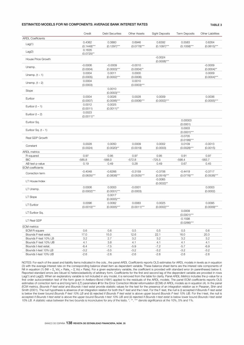
the estimation results for the ardl models of average bank interest rates are presented
in table 3. for this set of models, the most relevant control for the state of the business
17 the negative effect of interbank rates on credit growth is imposed as a requisite on the set of admissible specifications, but we do not impose linear or non-linear specifications, with the final estimated model produced as result of the model selection methodology in section 5.2. the signs of interbank rate coefficients on the rest of models for balance sheet growth are not constrained. see annex a.
6.2 estimated models for
average iNterest rates
BANCO DE ESPAÑA 138 REVISTA DE ESTABILIDAD FINANCIERA, NÚM. 35
NOTES: For each of the asset and liability items indicated in the cols., the panel ARDL Coefficients reports OLS estimates for ARDL models in levels as in equation (3) with the average interest rate on the corresponding balance sheet item as dependent variable. These balance sheet items are the interest rate components of NII in equation (1) (NII = Σa Vola × Ratea – Σl Voll × Ratel). For a given explanatory variable, the coefficient is provided with standard error (in parentheses) below it. Reported standard errors are robust to heterocedasticity of arbitrary form. Coefficients for the first and second lag of the dependent variable are provided in rows Lag(1) and Lag(2). When an explanatory variable is not included in any model, it is removed from the table for clarity. Panel ARDL Metrics includes the p-value for a first order autocorrelation test of the form given in Arellano-Bond (1991) applied to the residuals of the ARDL models. The panel ECM coefficients reports OLS estimates of correction term α and long term (LT) parameters 𝜽𝜽 for the Error Correction Model reformulation (ECM) of ARDL models as in equation (4). In the panel ECM metrics, Bounds F-test estat and Bounds t-test estat provide statistic values for the test for the presence of an integration relation as in Pesaran, Shin and Smith (2001). The null hypothesis is absence of an integration relation for both the F-test and the t-test. For the F-test, the null is (i) accepted if Bounds F-test estat is below the lower bound Bounds F-test 10% LB and (ii) rejected if Bounds F-test estat is above upper bound Bounds F-test 10% UB. For the t-test, the null is accepted if Bounds t-test estat is above the upper bound Bounds t-test 10% UB and (ii) rejected if Bounds t-test estat is below lower bound Bounds l-test estat 10% LB. A statistic value between the two bounds is inconclusive for any of the tests. *, **, *** denote significance at the 10%, 5% and 1%.
Credit Debt Securities Other Assets Sight Deposits Term Deposits Other Liabilities
ARDL Coefficients0.4362 0.3860 0.6946 0.6392 0.5583 0.6264(0.1448)*** (0.1297)*** (0.0778)*** (0.1097)*** (0.1058)*** (0.0615)***0.1635(0.0725)**
-0.0024(0.0008)***
9000.0-0100.0-9000.0-6000.0-**)4000.0(**)4000.0(***)3000.0()4000.0(
9000.00000.01100.04000.0***)4000.0()6000.0(***)2000.0()5000.0(
0100.04000.0***)3000.0()3000.0(
0.0010(0.0003)***
6300.09000.08200.06200.04000.0***)5000.0(***)2000.0(***)6000.0(***)6000.0()7000.0(
0.0012 0.0025(0.0011) (0.0011)**0.0023(0.0011)**
0.00003(0.0001)0.0003(0.0001)***-0.0705(0.0199)***
0.0028 0.0050 0.0009 0.0002 0.0109 -0.0013(0.0024) (0.0020)** (0.0019) (0.0003) (0.0028)*** (0.0015)
ARDL metrics79.019.059.079.059.079.0derauqs-R
7.385-4.895-5.527-8.275-0.885-8.585-CIB 54.076.094.082.094.091.0eulav-p tset BA
ECM coefficients-0.4048 -0.6266 -0.3159 -0.3706 -0.4419 -0.3717(0.0635)*** (0.0838)*** (0.0535)*** (0.0516)*** (0.0776)*** (0.0538)***
-0.0065(0.0032)**
3000.01000.0-3000.06000.0)2000.0()3000.0(***)1000.0(***)2000.0(
0.0017(0.0005)***
5900.05200.03800.02800.06900.0***)9000.0(***)2000.0(***)1100.0(***)5000.0(***)0100.0(
0.0009(0.0001)***-0.1598(0.0266)***
ECM metrics6.05.05.05.06.06.0erauqs-R MCE 3.020.611.226.210.510.71.tatse tset-F sdnuoB 2.32.32.32.37.22.3BL %01 tset-F sdnuoB 1.41.41.41.48.31.4BU %01 tset-F sdnuoB 9.6-7.5-2.7-9.5-5.7-4.6-.tatse tset-t sdnuoB 2.3-2.3-2.3-2.3-5.3-2.3-BL %01 tset-t sdnuoB 6.2-6.2-6.2-6.2-6.2-6.2-BU %01 tset-t sdnuoB
Euribor (t – 1)
Unemp.
Lag(1)
Lag(2)
House Price Growth
LT Euribor Sq.
LT Real GDP
LT Euribor
Unemp. (t – 1)
Unemp. (t – 2)
Slope
Euribor
Euribor (t – 2)
Euribor Sq.
Euribor Sq. (t – 1)
Real GDP Growth
Correction term
LT House Index
LT Unemp.
LT Slope
Constant
ESTIMATED MODELS FOR NII COMPONENTS: AVERAGE BANK INTEREST RATES TABLE 3
BANCO DE ESPAÑA 139 REVISTA DE ESTABILIDAD FINANCIERA, NÚM. 35
cycle is unemployment, which enters the specifications for the interest rates of credit, debt
securities holdings, rest of assets and rest of liabilities. the use of house price growth and
gdp growth provides parsimonious specifications for the interest rates on sight and term
deposits. as in the models for volume growth, the ar(1) specification prevail over the
ar(2) alternative, which applies only to the model for average interest rate earned on bank
credit.
the 12 month euribor enters linearly all the interest rate models except that of the interest rate
on term deposits, where it presents a non-linear lagged positive effect. the higher cost of
market financing implied by a higher 12 month euribor is translated more strongly to the cost
of term deposits when the interest rate level is high. this result is consistent with the
compression of profit margins on term deposit funds as interest rates near the zero level.
for the remaining categories of assets and liabilities, changes in reference interest rate are
translated linearly to their corresponding average interest rates. for traditional bank credit
products, this translation is lagged with a high and significant coefficient being applied to
the second lag of the 12 month euribor. there is also a lagged reaction in the debt securities
holding category, whereas the relation between 12 month euribor and the rest of assets
and liabilities (interbank positions, wholesale financing products, etc.) is contemporaneous,
plausibly reflecting the shorter maturities in these categories.
examining the ecm reparametrization of the bank average interest rate models, we see
that the estimated speed of adjustment α for different interest rates is quite comparable
across balance sheet categories, as opposed to the more heterogeneous pattern found for
the balance sheet growth models. the exception to this homogenous pattern is the interest
rate on debt securities holdings, which presents a faster speed of adjustment than the rest of
the models. The long run coefficients on the 12 month Euribor, or the squared term of 12 month
euribor in the model for interest rate on term deposits, are significant and point to the
existence of a long term relation between the interbank rate and the average interest rates
on different bank balance sheet categories. as regards cointegration, the pesaran-shin-
smith bound tests in table 3 strongly point to the presence of an integration relation. both
the f-test and the t-test reject the null hypothesis of no cointegration relation at the 10%
level in all cases.
the models implemented for ofbi and provisioning charges are presented in table 4. the
two models present some common elements, such as the inclusion of ar(1) dynamics, a
purely non-linear effect of the 12 month euribor and the use of a single macro variable to
control for the state of the business cycle. additionally, the pesaran-shin-smith bound tests
support the presence of an integration relation with macro and interest rate controls for both
of these variables, with both tests rejecting the null hypothesis. however, there are also
significant differences between the two models. the effect of changes in 12 month euribor
on provisioning charges are more persistent due to both a higher ar(1) coefficient and the
absence of compensating lagged terms (the first and second lag of 12 month euribor have
opposing signs and comparable magnitude in the model for ofbi). the effect of the business
cycle is controlled with the unemployment variable in the model for ofbi, whereas house
price growth (a variable related to general economic conditions, but also specifically to the
value of real estate collateral) is applied in the model for provisioning charges.
We perform in this subsection a dynamic sensitivity analysis of bank income components
to market interest rates by introducing a temporary 100bp one-period shock to the 12
month euribor at the start date of the 3 year study horizon. this is a pure sensitivity analysis
6.3 estimated models for
other baNk iNcome:
ofbi aNd provisioNiNg
charges
6.4 baNk iNcome dyNamics
aNd iNterest rate
shocks

BANCO DE ESPAÑA 140 REVISTA DE ESTABILIDAD FINANCIERA, NÚM. 35
NOTES: For each of the P&L income categories indicated in the cols., the panel ARDL Coefficients reports OLS estimates for ARDL models in levels as in equation (3) with the year-on-year growth rate of the corresponding P&L category as dependent variable. For a given explanatory variable, the coefficient is provided with standard error (in parentheses) below it. Reported standard errors are robust to heterocedasticity of arbitrary form. Coefficients for the first and second lag of the dependent variable are provided in rows Lag(1) and Lag(2). When an explanatory variable is not included in any model, it is removed from the table for clarity. Panel ARDL Metrics includes the p-value for a first order autocorrelation test of the form given in Arellano-Bond (1991) applied to the residuals of the ARDL models. The panel ECM coefficients reports OLS estimates of correction term α and long term (LT) parameters 𝜽𝜽 for the Error Correction Model reformulation (ECM) of ARDL models as in equation (4). In the panel ECM metrics, Bounds F-test estat and Bounds t-test estat provide statistic values for the test for the presence of an integration relation as in Pesaran, Shin and Smith (2001). The null hypothesis is absence of an integration relation for both the F-test and the t-test. For the F-test, the null is (i) accepted if Bounds F-test estat is below the lower bound Bounds F-test 10% LB and (ii) rejected if Bounds F-test estat is above upper bound Bounds F-test 10% UB. For the t-test, the null is accepted if Bounds t-test estat is above the upper bound Bounds t-test 10% UB and (ii) rejected if Bounds t-test estat is below lower bound Bounds l-test estat 10% LB. A statistic value between the two bounds is inconclusive for any of the tests. *, **, *** denote significance at the 10%, 5% and 1%.
egrahC noisivorPemocnI BFO
ARDL Coefficients
0106.04513.0
***)0341.0(***)1711.0(
-2.0561
(0.6482)***
-0.0082
(0.0047)*
9950.07200.0
***)3810.0()2800.0(
0.0226
(0.0143)
-0.0290
(0.0095)***
3951.0-1522.0
)4501.0(**)5111.0(
ARDL metrics
R-squared 28.005.0
BIC 0.783.74-
47.075.0eulav-p tset BA
ECM coefficients
0993.0-6556.0-
***)4380.0(***)5901.0(
-5.1537
(1.7662)***
-0.0132
(0.0062)**
LT Slope
LT Euribor
2051.01700.0-
***)0520.0()2500.0(
LT Real GDP
ECM metrics
4.04.0erauqs-R MCE
6.94.31.tatse tset-F sdnuoB
2.32.3BL %01 tset-F sdnuoB
1.41.4BU %01 tset-F sdnuoB
8.4-0.6-.tatse tset-t sdnuoB
2.3-2.3-BL %01 tset-t sdnuoB
6.2-6.2-BU %01 tset-t sdnuoB
LT Euribor Sq.
LT House Index
Lag(1)
House Price Growth
Correction term
LT Unemp.
Unemp.
Euribor Sq.
Euribor Sq. (t – 1)
Euribor Sq. (t – 2)
Constant
ESTIMATED MODELS FOR ADDITIONAL BANK INCOME COMPONENTS TABLE 4

BANCO DE ESPAÑA 141 REVISTA DE ESTABILIDAD FINANCIERA, NÚM. 35
under ceteris paribus conditions rather than a scenario analysis, as we keep constant
the remaining factors of the model (macro variables and error term) when we introduce the
one-period shock on interest rates. this choice of analytical method seeks exclusively to
isolate the sensitivity of bank income to a perturbation of interest rates.18
the sample covering 2000-2015 presents periods with very different interest rate levels and
business cycle conditions. given this historical sample and the finding of non-linear terms
for interest rates in several of the estimated models in subsections 6.1-6.3, the sensitivity of
bank income to interest rates can be expected to differ over different subperiods. thus, we
perform the exercise for both the periods 2007-2009 (including a severe economic downturn
and the highest interest rate level in sample) and 2013-2015 (a period of economic recovery
combined with the lowest level of interest rates in the sample).
for each modelled variable, we compute first the effect of the 100bp one-period shock on
the initial quarter. then, we measure the effect of the shock propagation through the
autoregressive terms of the modelled variable and, when applicable, the lagged terms of
the euribor variables. finally, we take the difference between the generated path induced
by the shock and the historical path observed in the data19. We measure in this way the
impact of the euribor shock on each of the 12 quarters of the 3 year period of analysis. for
Nii, we present both the impact of the temporary interest rate shock on each of its volume
and interest rate components, and the figure of Nii itself that results from aggregating
these components: NII Vol Rate Vol Ratea aa l ll� � � �� � (for asset and liability categories
a and l). in order to infer a confidence interval around the estimated effect of the shock,
we employ a bootstrap methodology. We take a 1,000 draws of the coefficients of the
different estimated models and recompute the effect of the 100bp shock on all the variables
of interest.20 this provides a bootstrapped distribution of the effect of the 12 month euribor
shock on all the components of bank income.
in year 2007, the 12 month euribor was already above the 4% level, a high level relative to
the sample average value of 2.45%, and bank provisioning charges were escalating
quickly. thus, a 100bp shock to 12 month euribor can be a priori expected to put pressure
on the debt servicing capacity of bank borrowers and push further the cost of financing for
banks. the estimated models allow to quantify more precisely the effect of this euribor
shock.
chart 2 presents the effect of the transitory shock on the year-on-year growth of different
assets and liabilities, measured as difference of counterfactual and actual growth rates.
credit growth is slowed down significantly as result of the 100bp shock to 12 month
euribor. despite the absence of significant initial response on Q1 2007, the decline of
1.3 pp on Q2 2007 is sizeable and confidence intervals stay in the negative territory for the
rest of the horizon of analysis. The effect on Q4 2009 is still –0.5 pp with negative confidence
18 alternative analysis could be constructed, with a staggered calendar of rate changes and permanent changes to the level of the reference rate. additionally, a consistent macro scenario (with macro variables adapted to the alternative interest rate path) could be applied to obtain the full net effect on bank profitability beyond the pure interest rate effect. in this article, we limit the analysis to this pure rate effect and we use the one period 100bp change as a natural unit of reference.
19 macro variables other than the 12 month euribor take the same values in the shock-generated path and in the historical path, so the difference between both paths only reflects the effect of the shock to the 12 month euribor on the initial quarter, which propagate over several quarters because of the autoregressive structure on the dependent variable and the 12 month euribor itself.
20 We use the estimated coefficients and their associated variance covariance matrix for each ardl model in levels to obtain normal random draws.
6.4.1 dynamic effect of interest
rate shocks in 2007-2009

BANCO DE ESPAÑA 142 REVISTA DE ESTABILIDAD FINANCIERA, NÚM. 35
interval, indicating that the effect on credit does not dissipate quickly. the effect on the
growth rate of the rest of assets category (covering for example interbank exposures) is
also negative, with a big initial decline of –2.7 pp on Q1 2007 that dissipates rapidly
(–0.2 pp on Q1 2008 and –0.002 pp on Q4 2009). On the contrary, the volume of debt
securities holdings increases as result of the shock, even though the increase is only
significant over the first four quarters of analysis (Q1 2007 – Q4 2007). as the 12 month
euribor goes up, we observe a substitution of traditional bank credit towards debt securities
holdings.
on the liability side, we observe substitution from sight to term deposits, which is natural
given the rise in their reference interest rate. the confidence intervals for the reduction in
growth of sight deposits stay in the negative region from Q1 2007 to Q2 2008, whereas the
confidence intervals for the impact on term deposit growth are in the positive region, but
they marginally contact zero. the effect on the rest of liabilities is clearly negative, with an
initial decline of 0.95 pp that persists as significant for four quarters. The additional market
tension introduced by the interest rate shock, plausibly leads to a decline of market financing
and greater reliance on term deposits.
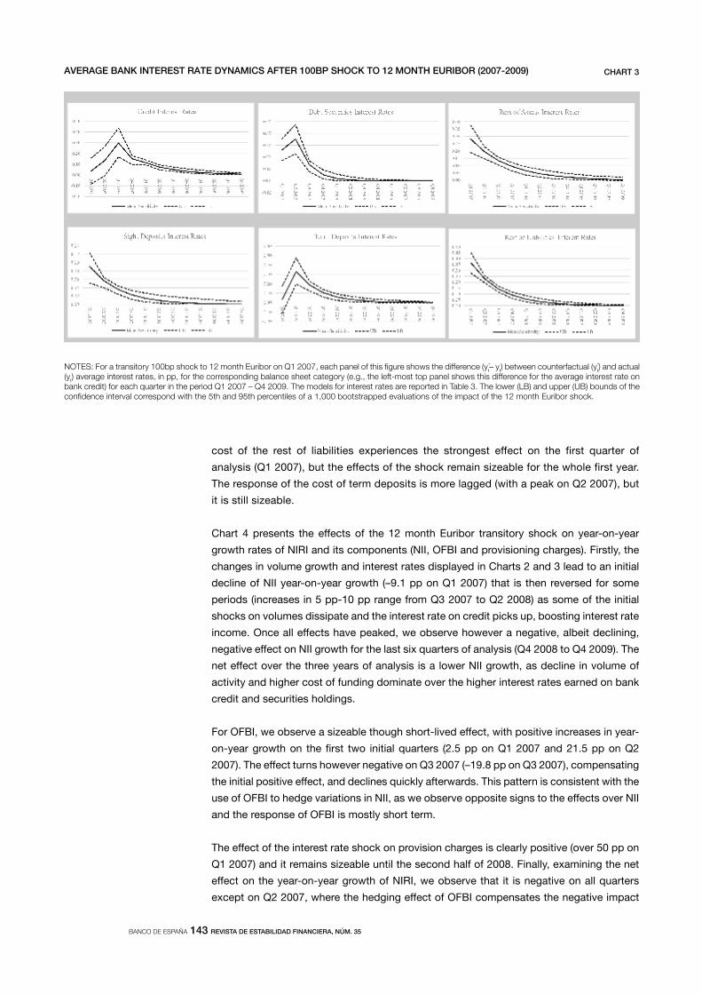
chart 3 displays the effect of the transitory 100bp shock to 12 month euribor on the
average interest rates corresponding to the different asset and liability categories. the
rise in the 12 month euribor increases the levels of all bank interest rates, with a maximum
effect of the shock in a given quarter in the 0.3 pp-0.4 pp range for all the series, except
sight deposits (with maximum initial reaction of 0.1 pp that dissipates quickly). The
differences in the speed of adjustment of different categories are relevant to understand
the net changes in Nii growth over time. on the asset side, it takes up to three quarters
to observe a significant positive effect on credit interest rates, whereas the effect is
immediately positive on the debt securities and rest of assets categories, which are
more directly linked to wholesale financial markets. on the liability side, the interest rate
NOTES: For a transitory 100bp shock to 12 month Euribor on Q1 2007, each panel of this figure shows the difference (yt – yt ) between counterfactual (yt) and
actual (yt) year-on-year growth rates for the corresponding balance sheet category (e.g., the left-most top panel shows this difference for bank credit growth rate) for each quarter t in the period Q1 2007 – Q4 2009. The models for balance sheet categories are reported in Table 2. The lower (LB) and upper (UB) bounds of the confidence interval correspond with the 5th and 95th percentiles of the distribution of a 1,000 bootstrapped evaluations of the impact of the 12 month Euribor shock.
BALANCE SHEET GROWTH DYNAMICS AFTER 100BP SHOCK TO 12 MONTH EURIBOR (2007-2009) CHART 2
* *
BANCO DE ESPAÑA 143 REVISTA DE ESTABILIDAD FINANCIERA, NÚM. 35
cost of the rest of liabilities experiences the strongest effect on the first quarter of
analysis (Q1 2007), but the effects of the shock remain sizeable for the whole first year.
the response of the cost of term deposits is more lagged (with a peak on Q2 2007), but
it is still sizeable.
chart 4 presents the effects of the 12 month euribor transitory shock on year-on-year
growth rates of Niri and its components (Nii, ofbi and provisioning charges). firstly, the
changes in volume growth and interest rates displayed in charts 2 and 3 lead to an initial
decline of NII year-on-year growth (–9.1 pp on Q1 2007) that is then reversed for some
periods (increases in 5 pp-10 pp range from Q3 2007 to Q2 2008) as some of the initial
shocks on volumes dissipate and the interest rate on credit picks up, boosting interest rate
income. once all effects have peaked, we observe however a negative, albeit declining,
negative effect on Nii growth for the last six quarters of analysis (Q4 2008 to Q4 2009). the
net effect over the three years of analysis is a lower Nii growth, as decline in volume of
activity and higher cost of funding dominate over the higher interest rates earned on bank
credit and securities holdings.
for ofbi, we observe a sizeable though short-lived effect, with positive increases in year-
on-year growth on the first two initial quarters (2.5 pp on Q1 2007 and 21.5 pp on Q2
2007). The effect turns however negative on Q3 2007 (–19.8 pp on Q3 2007), compensating
the initial positive effect, and declines quickly afterwards. this pattern is consistent with the
use of ofbi to hedge variations in Nii, as we observe opposite signs to the effects over Nii
and the response of ofbi is mostly short term.
The effect of the interest rate shock on provision charges is clearly positive (over 50 pp on
Q1 2007) and it remains sizeable until the second half of 2008. finally, examining the net
effect on the year-on-year growth of Niri, we observe that it is negative on all quarters
except on Q2 2007, where the hedging effect of ofbi compensates the negative impact
NOTES: For a transitory 100bp shock to 12 month Euribor on Q1 2007, each panel of this figure shows the difference (yt– yt) between counterfactual (yt) and actual (yt) average interest rates, in pp, for the corresponding balance sheet category (e.g., the left-most top panel shows this difference for the average interest rate on bank credit) for each quarter in the period Q1 2007 – Q4 2009. The models for interest rates are reported in Table 3. The lower (LB) and upper (UB) bounds of the confidence interval correspond with the 5th and 95th percentiles of a 1,000 bootstrapped evaluations of the impact of the 12 month Euribor shock.
AVERAGE BANK INTEREST RATE DYNAMICS AFTER 100BP SHOCK TO 12 MONTH EURIBOR (2007-2009) CHART 3
* *

BANCO DE ESPAÑA 144 REVISTA DE ESTABILIDAD FINANCIERA, NÚM. 35
on other profit components. it must be noted however that the confidence interval for
quarters in the first half of the study period crosses zero, reducing the significance of the
effect of the 12 month euribor on Niri growth. starting on Q3 2008, the confidence
intervals stay consistently below zero, indicating a significant effect of the shock in these
latter quarters. as the positive effects on Nii growth disappear, the negative effects on
profitability through lower Nii and higher provision charges become dominant and bring
down Niri growth.
in year 2013, the spanish economy was in recession and the provisioning charges of
banks remained at high historical levels, but the 12 month euribor was at a relatively low
level (approx. 1%) and the following two years would present a path of positive gdp
growth and declining interest rates. under these different conditions relative to the 2007-
2009 period, the 100bp euribor shock would introduce a priori less pressure on the profit
margins of banks. We verify whether this is the case with the model projections.
chart 5 presents the effect on the growth of different balance sheet categories of a
transitory 100bp shock to 12 month euribor on Q1 2013. as in subsection 6.4.1, the impact
on credit growth is negative and persistent, but the effect is weaker. for example, the initial
effect (Q1 2013) is again insignificant and the slowing of credit growth begins in the second
quarter (Q2 2013) with a shock of –0.3 pp, which is smaller than the shock of –1.3 pp on
Q2 2007 measured in the previous experiment. given that the model implemented for debt
securities is linear in 12 month euribor, the projected path of this variable is positive and
coincides with that of the previous experiment in subsection 6.4.1. interestingly, the effect
on the growth of the rest of assets is now found to be positive, though the wide confidence
intervals do not allow to preclude a null effect. based on the results of the two experiments,
the increase in 12 month euribor contracts (expands) this form of exposure when this
reference rate is at high (low) levels.
6.4.2 dynamic effect of interest
rate shocks in 2013-2015
NOTES: For a 100bp shock to 12 month Euribor on Q1 2007, each panel of this figure shows the difference (yt– yt) between counterfactual (yt) and actual (yt) year-on-year growth rates for the corresponding P&L component (e.g., the left-most top panel shows this difference for NII growth rate) for each quarter t in the period Q1 2007 – Q4 2009. The lower (LB) and upper (UB) bounds of the confidence interval correspond with the 5th and 95th percentiles of the distribution of a 1,000 bootstrapped evaluations of the impact of the 12 month Euribor shock. The following variable definitions apply: NII (Net Interest Income), OFBI (Other Financial and Banking Income) and NIRI (Net Interest Related Income). NII is modelled as a function of balance sheet growth and interest rates according to equation (1), OFBI and provision charges are modelled directly, and NIRI is modelled as function of the other variables based on equation (2).
BANK PROFITABILITY DYNAMICS AFTER 100BP SHOCK TO 12 MONTH EURIBOR (2007-2009) CHART 4
* *
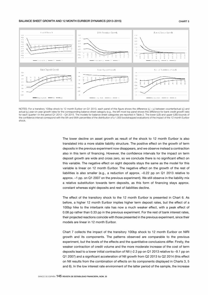
BANCO DE ESPAÑA 145 REVISTA DE ESTABILIDAD FINANCIERA, NÚM. 35
the lower decline on asset growth as result of the shock to 12 month euribor is also
translated into a more stable liability structure. the positive effect on the growth of term
deposits in the previous experiment now disappears, and we observe instead a contraction
also in this term of financing. however, the confidence intervals for the impact on term
deposit growth are wide and cross zero, so we conclude there is no significant effect on
this variable. the negative effect on sight deposits stays the same as the model for this
variable is linear on 12 month euribor. the negative effect on the growth of the rest of
liabilities is also smaller (e.g., a reduction of approx. –0.22 pp on Q1 2013 relative to
approx. –1 pp. on Q1 2007 on the previous experiment). We still observe in the liability mix
a relative substitution towards term deposits, as this form of financing stays approx.
constant whereas sight deposits and rest of liabilities decline.
the effect of the transitory shock to the 12 month euribor is presented in chart 6. as
before, a higher 12 month euribor implies higher term deposit rates, but the effect of a
100bp hike to the interbank rate has now a much weaker effect, with a peak effect of
0.08 pp rather than 0.33 pp in the previous experiment. For the rest of bank interest rates,
their projected reactions coincide with those presented in the previous experiment, since their
models are linear in 12 month euribor.
chart 7 collects the impact of the transitory 100bp shock to 12 month euribor on Niri
growth and its components. the patterns observed are comparable to the previous
experiment, but the levels of the effects and the quantitative conclusions differ. firstly, the
weaker contraction of credit volume and the more moderate increase of the cost of term
deposits lead to a lower initial contraction of NII (–2.3 pp on Q1 2013 relative to –9.1 pp on
Q1 2007) and a significant acceleration of Nii growth from Q2 2013 to Q2 2014 (this effect
on Nii results from the combination of effects on its components displayed in charts 3, 5
and 6). in the low interest rate environment of the latter period of the sample, the increase
NOTES: For a transitory 100bp shock to 12 month Euribor on Q1 2013, each panel of this figure shows the difference (yt – yt) between counterfactual (yt) and actual (yt) year-on-year growth rates for the corresponding balance sheet category (e.g., the left-most top panel shows this difference for bank credit growth rate) for each quarter t in the period Q1 2013 – Q4 2015. The models for balance sheet categories are reported in Table 2. The lower (LB) and upper (UB) bounds of the confidence interval correspond with the 5th and 95th percentiles of the distribution of a 1,000 bootstrapped evaluations of the impact of the 12 month Euribor shock.
BALANCE SHEET GROWTH AND 12 MONTH EURIBOR DYNAMICS (2013-2015) CHART 5
* *
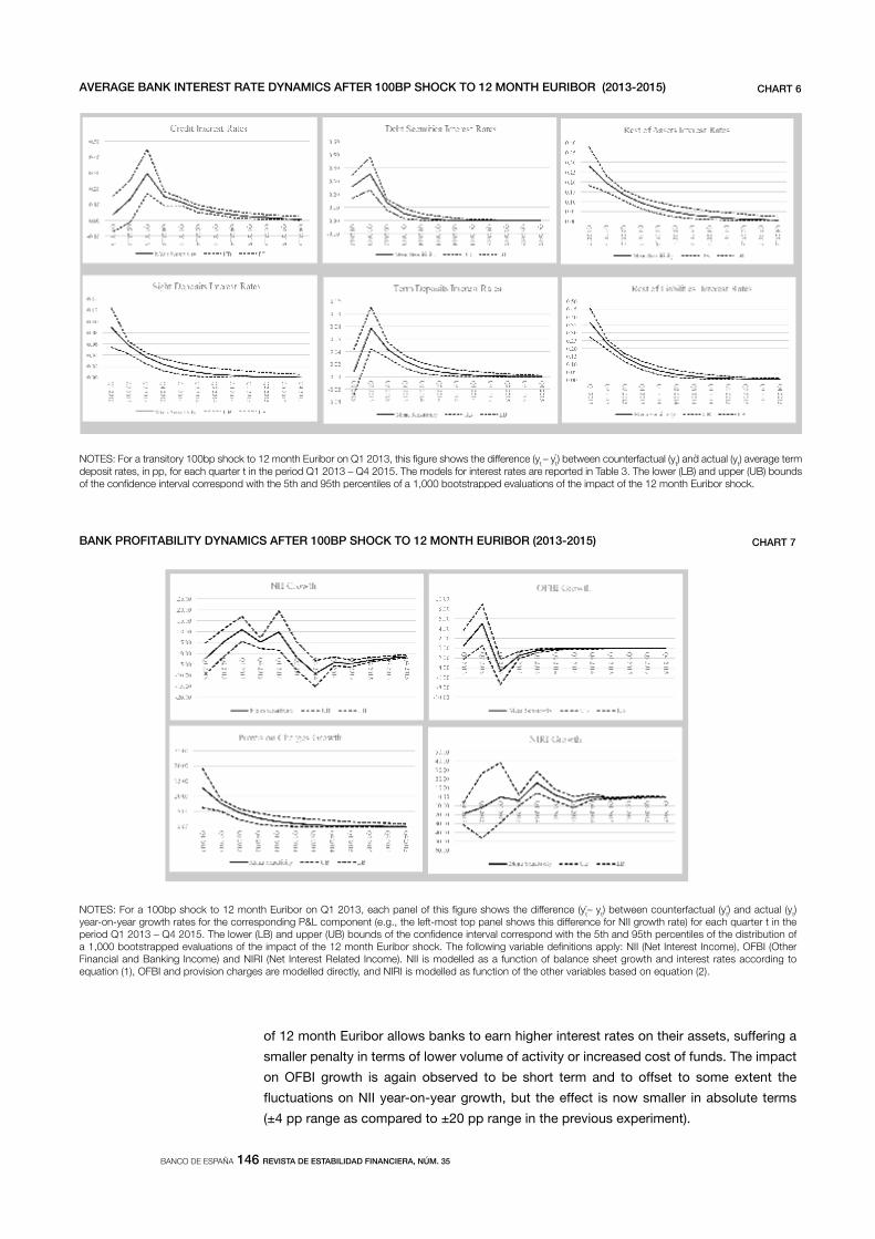
BANCO DE ESPAÑA 146 REVISTA DE ESTABILIDAD FINANCIERA, NÚM. 35
of 12 month euribor allows banks to earn higher interest rates on their assets, suffering a
smaller penalty in terms of lower volume of activity or increased cost of funds. the impact
on ofbi growth is again observed to be short term and to offset to some extent the
fluctuations on Nii year-on-year growth, but the effect is now smaller in absolute terms
(±4 pp range as compared to ±20 pp range in the previous experiment).
NOTES: For a transitory 100bp shock to 12 month Euribor on Q1 2013, this figure shows the difference (yt – yt) between counterfactual (yt) and actual (yt) average term
deposit rates, in pp, for each quarter t in the period Q1 2013 – Q4 2015. The models for interest rates are reported in Table 3. The lower (LB) and upper (UB) bounds of the confidence interval correspond with the 5th and 95th percentiles of a 1,000 bootstrapped evaluations of the impact of the 12 month Euribor shock.
AVERAGE BANK INTEREST RATE DYNAMICS AFTER 100BP SHOCK TO 12 MONTH EURIBOR (2013-2015) CHART 6
* *
NOTES: For a 100bp shock to 12 month Euribor on Q1 2013, each panel of this figure shows the difference (yt– yt) between counterfactual (yt) and actual (yt) year-on-year growth rates for the corresponding P&L component (e.g., the left-most top panel shows this difference for NII growth rate) for each quarter t in the period Q1 2013 – Q4 2015. The lower (LB) and upper (UB) bounds of the confidence interval correspond with the 5th and 95th percentiles of the distribution of a 1,000 bootstrapped evaluations of the impact of the 12 month Euribor shock. The following variable definitions apply: NII (Net Interest Income), OFBI (Other Financial and Banking Income) and NIRI (Net Interest Related Income). NII is modelled as a function of balance sheet growth and interest rates according to equation (1), OFBI and provision charges are modelled directly, and NIRI is modelled as function of the other variables based on equation (2).
BANK PROFITABILITY DYNAMICS AFTER 100BP SHOCK TO 12 MONTH EURIBOR (2013-2015) CHART 7
* *
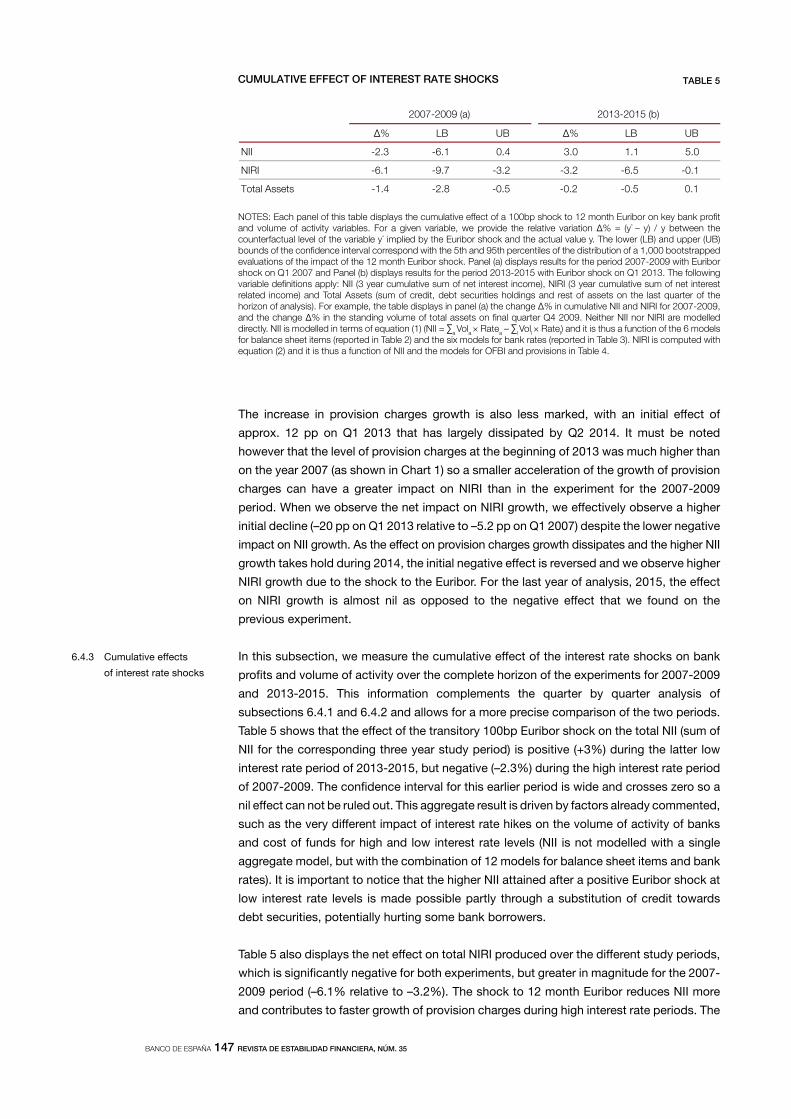
BANCO DE ESPAÑA 147 REVISTA DE ESTABILIDAD FINANCIERA, NÚM. 35
the increase in provision charges growth is also less marked, with an initial effect of
approx. 12 pp on Q1 2013 that has largely dissipated by Q2 2014. It must be noted
however that the level of provision charges at the beginning of 2013 was much higher than
on the year 2007 (as shown in chart 1) so a smaller acceleration of the growth of provision
charges can have a greater impact on Niri than in the experiment for the 2007-2009
period. When we observe the net impact on Niri growth, we effectively observe a higher
initial decline (–20 pp on Q1 2013 relative to –5.2 pp on Q1 2007) despite the lower negative
impact on Nii growth. as the effect on provision charges growth dissipates and the higher Nii
growth takes hold during 2014, the initial negative effect is reversed and we observe higher
Niri growth due to the shock to the euribor. for the last year of analysis, 2015, the effect
on Niri growth is almost nil as opposed to the negative effect that we found on the
previous experiment.
in this subsection, we measure the cumulative effect of the interest rate shocks on bank
profits and volume of activity over the complete horizon of the experiments for 2007-2009
and 2013-2015. this information complements the quarter by quarter analysis of
subsections 6.4.1 and 6.4.2 and allows for a more precise comparison of the two periods.
table 5 shows that the effect of the transitory 100bp euribor shock on the total Nii (sum of
Nii for the corresponding three year study period) is positive (+3%) during the latter low
interest rate period of 2013-2015, but negative (–2.3%) during the high interest rate period
of 2007-2009. the confidence interval for this earlier period is wide and crosses zero so a
nil effect can not be ruled out. this aggregate result is driven by factors already commented,
such as the very different impact of interest rate hikes on the volume of activity of banks
and cost of funds for high and low interest rate levels (Nii is not modelled with a single
aggregate model, but with the combination of 12 models for balance sheet items and bank
rates). it is important to notice that the higher Nii attained after a positive euribor shock at
low interest rate levels is made possible partly through a substitution of credit towards
debt securities, potentially hurting some bank borrowers.
table 5 also displays the net effect on total Niri produced over the different study periods,
which is significantly negative for both experiments, but greater in magnitude for the 2007-
2009 period (–6.1% relative to –3.2%). the shock to 12 month euribor reduces Nii more
and contributes to faster growth of provision charges during high interest rate periods. the
6.4.3 cumulative effects
of interest rate shocks
NOTES: Each panel of this table displays the cumulative effect of a 100bp shock to 12 month Euribor on key bank profit and volume of activity variables. For a given variable, we provide the relative variation ∆% = (y* – y) / y between the counterfactual level of the variable y* implied by the Euribor shock and the actual value y. The lower (LB) and upper (UB) bounds of the confidence interval correspond with the 5th and 95th percentiles of the distribution of a 1,000 bootstrapped evaluations of the impact of the 12 month Euribor shock. Panel (a) displays results for the period 2007-2009 with Euribor shock on Q1 2007 and Panel (b) displays results for the period 2013-2015 with Euribor shock on Q1 2013. The following variable definitions apply: NII (3 year cumulative sum of net interest income), NIRI (3 year cumulative sum of net interest related income) and Total Assets (sum of credit, debt securities holdings and rest of assets on the last quarter of the horizon of analysis). For example, the table displays in panel (a) the change ∆% in cumulative NII and NIRI for 2007-2009, and the change ∆% in the standing volume of total assets on final quarter Q4 2009. Neither NII nor NIRI are modelled directly. NII is modelled in terms of equation (1) (NII = ∑a Vola × Ratea – ∑l Voll × Ratel) and it is thus a function of the 6 models for balance sheet items (reported in Table 2) and the six models for bank rates (reported in Table 3). NIRI is computed with equation (2) and it is thus a function of NII and the models for OFBI and provisions in Table 4.
Δ% LB UB Δ% LB UB
0.51.10.34.01.6-3.2-IIN
1.0-5.6-2.3-2.3-7.9-1.6-IRIN
Total Assets -1.4 -2.8 -0.5 -0.2 -0.5 0.1
)b( 5102-3102 )a( 9002-7002
CUMULATIVE EFFECT OF INTEREST RATE SHOCKS TABLE 5
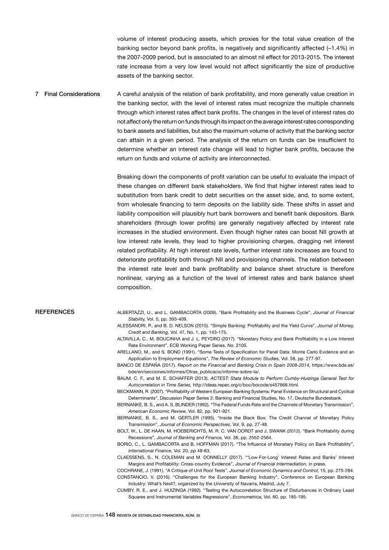
BANCO DE ESPAÑA 148 REVISTA DE ESTABILIDAD FINANCIERA, NÚM. 35
volume of interest producing assets, which proxies for the total value creation of the
banking sector beyond bank profits, is negatively and significantly affected (–1.4%) in
the 2007-2009 period, but is associated to an almost nil effect for 2013-2015. the interest
rate increase from a very low level would not affect significantly the size of productive
assets of the banking sector.
a careful analysis of the relation of bank profitability, and more generally value creation in
the banking sector, with the level of interest rates must recognize the multiple channels
through which interest rates affect bank profits. the changes in the level of interest rates do
not affect only the return on funds through its impact on the average interest rates corresponding
to bank assets and liabilities, but also the maximum volume of activity that the banking sector
can attain in a given period. the analysis of the return on funds can be insufficient to
determine whether an interest rate change will lead to higher bank profits, because the
return on funds and volume of activity are interconnected.
breaking down the components of profit variation can be useful to evaluate the impact of
these changes on different bank stakeholders. We find that higher interest rates lead to
substitution from bank credit to debt securities on the asset side, and, to some extent,
from wholesale financing to term deposits on the liability side. these shifts in asset and
liability composition will plausibly hurt bank borrowers and benefit bank depositors. bank
shareholders (through lower profits) are generally negatively affected by interest rate
increases in the studied environment. even though higher rates can boost Nii growth at
low interest rate levels, they lead to higher provisioning charges, dragging net interest
related profitability. at high interest rate levels, further interest rate increases are found to
deteriorate profitability both through Nii and provisioning channels. the relation between
the interest rate level and bank profitability and balance sheet structure is therefore
nonlinear, varying as a function of the level of interest rates and bank balance sheet
composition.
ALBERTAZZI, U., and l. gambacorta (2009). “bank profitability and the business cycle”, Journal of Financial Stability, vol. 5, pp. 393-409.
alessaNdri, p., and b. d. NelsoN (2015). “simple banking: profitability and the yield curve”, Journal of Money, Credit and Banking, vol. 47, No. 1, pp. 143-175.
altavilla, c., m. bouciNha and J. l. peydro (2017). “monetary policy and bank profitability in a low interest rate environment”, ecb Working paper series, No. 2105.
arellaNo, m., and s. boNd (1991). “some tests of specification for panel data: monte carlo evidence and an application to employment equations”, The Review of Economic Studies, vol. 58, pp. 277-97.
baNco de espaÑa (2017). Report on the Financial and Banking Crisis in Spain 2008-2014, https://www.bde.es/bde/en/secciones/informes/otras_publicacio/informe-sobre-la/.
baum, c. f., and m. e. schaffer (2013). ACTEST: Stata Module to Perform Cumby-Huizinga General Test for Autocorrelation in Time Series, http://ideas.repec.org/c/boc/bocode/s457668.html.
beckmaNN, r. (2007). “profitability of Western european banking systems: panel evidence on structural and cyclical determinants”, discussion Paper Series 2: Banking and Financial Studies, No. 17, deutsche bundesbank.
berNaNke, b. s., and a. s. bliNder (1992). “the federal funds rate and the channels of monetary transmission”, American Economic Review, vol. 82, pp. 901-921.
berNaNke, b. s., and m. gertler (1995). “inside the black box: the credit channel of monetary policy transmission”, Journal of Economic Perspectives, vol. 9, pp. 27-48.
bolt, W., l. de haaN, m. hoeberichts, m. r. c. vaN oordt and J. sWaNk (2012). “bank profitability during recessions”, Journal of Banking and Finance, vol. 36, pp. 2552-2564.
borio, c., l. gambacorta and b. hoffmaN (2017). “the influence of monetary policy on bank profitability”, International Finance, vol. 20, pp 48-63.
claesseNs, s., N. colemaN and m. doNNelly (2017). “‘low-for-long’ interest rates and banks’ interest margins and profitability: cross-country evidence”, Journal of Financial Intermediation, in press.
cochraNe, J. (1991). “a critique of unit root tests”, Journal of Economic Dynamics and Control, 15, pp. 275-284.coNstaNcio, v. (2016). “challenges for the european banking industry”, conference on european banking
industry: What’s Next?, organized by the university of Navarra, madrid, July 7.cumby, r. e., and J. HUIZINGA (1992). “testing the autocorrelation structure of disturbances in ordinary least
squares and instrumental variables regressions”, Econometrica, vol. 60, pp. 185-195.
7 Final Considerations
REFERENCES
BANCO DE ESPAÑA 149 REVISTA DE ESTABILIDAD FINANCIERA, NÚM. 35
demirgüÇ-kuNt, a., and H. HUIZINGA (1999). “determinants of commercial bank interest margins and profitability: some international evidence”, The World Bank Economic Review, vol. 13, No. 2, pp 379-408.
deyouNg, r., and k. p. rolaNd (2001). “product mix and earnings volatility at commercial banks: evidence from a degree of total leverage model”, Journal of Financial Intermediation, vol. 10, pp. 54-84.
dobbs, r., s. luNd, t. koller and a. shWayde (2013). QE and ultra-low interest rates: Distributional effects and risks, report by mckinsey global institute, November 2013.
duffie, d., l. saita and k. WaNg (2007). “multi-period corporate default prediction with stochastic covariates”, Journal of Financial Economics, vol. 83, pp. 635-665.
fischer, s. (2016). “Why are interest rates so low? causes and implications”, conference at the economic club of New york, New york, october 17.
FREIXAS, X., and J. c. rochet (2008). microeconomics of banking, mit press.gambacorta, l., and p. e. mistrulli (2004). “does bank capital affect lending behavior?”, Journal of Financial
Intermediation, vol. 13, pp. 436-457.gortoN, g., and r. roseN (1995). “banks and derivatives”, NBER Macroeconomics Annual, Vol. 10, pp. 299-339.heNry, J., and c. kok (2013). A Macro Stress Testing Framework for Assessing Systemic Risks in the Banking
Sector, ecb occasional paper series, No. 152.JIMÉNEZ, G., and J. meNcía ( 2009). “modelling the distribution of credit losses with observable and latent
factors”, Journal of Empiriral Finance, vol. 16, pp. 235-253.JIMÉNEZ, G., S. ONGENA, J. L. PEYDRÓ and J. sauriNa (2014). “hazardous times for monetary policy: What do
23 million bank loans say about the implementation of monetary policy?”, Econometrica, vol. 82, pp. 463-505.
JIMÉNEZ, G., and J. sauriNa (2006). “credit cycles, credit risk, and prudential regulati”, International Journal of Central Banking, vol. 2, No. 2, pp. 65-98.
kashyap, a. k., and J. c. steiN (2000). “What do a million observations on banks say about the transmission of monetary policy?”, American Economic Review, vol. 90, pp. 407-428.
kashyap, a., k., J. c. steiN and D. W. WILCOX (1993). “monetary policy and credit conditions: evidence from the composition of external finance”, American Economic Review, vol. 83, pp. 78-98.
kleiN, m. a. (1971). “a theory of the banking firm”, Journal of Money, Credit and Banking, vol. 3, pp. 205-218.KRIPFGANZ, S., and d. c. schNeider (2016). “ardl: stata module to estimate autoregressive distributed lag
models”, presented July 29, at the stata conference, chicago.kWiatkoWski, d., p. c. b. phillips, p. schmidt and y. shiN (1992). “testing the Null hypothesis of stationarity
against the alternative of a unit root: how sure are we that economic time series have a unit root?”, Journal of Econometrics, 54, pp. 159-178.
lehmaNN, h., and M. MANZ (2006). “the exposure of swiss banks to macroeconomic shocks - an empirical investigation”, swiss National bank Working paper, No. 2006-4.
lepetit, l., e. Nys, p. rous and A. TARAZI (2008). “bank income structure and risk: an empirical analysis of european banks”, Journal of Banking and Finance, vol. 32, pp. 1452-1467.
marcucci, J., and m. Quagliariello (2009). “asymmetric effects of the business cycle on bank credit risk”, Journal of Banking and Finance, vol. 33, pp. 1624-1635.
moNti, m. (1972). “deposit, credit and interest rate determination under alternative bank objectives”, in g. p. szego and k. shell (eds.), Mathematical Methods in Investment and Finance, amsterdam.
pesaraN, m. h., and y. shiN (1999). “an autoregressive distributed lag modelling approach to cointegration analysis”, in strom s (ed.), Econometrics and Economic Theory in the 20th Century: The Ragnar Frisch Centennial Symposium, chapter 11, cambridge university press, cambridge.
pesaraN, m. h., y. shiN and r. smith (2001). “bounds testing approaches to the analysis of level relationships”, Journal of Applied Econometrics, vol. 16, No. 3, pp. 289-326.
pesaraN, m. h., t. schuermaNN, b. J. treutler and s. m. WeiNer (2006). “macroeconomic dynamics and credit risk: a global perspective”, Journal of Money, Credit, and Banking, vol. 38, pp. 1211-1261.
purNaNdam, a. (2007). “interest rate derivatives at commercial banks: an empirical investigation”, Journal of Monetary Economics, vol. 54, pp. 1769-1808.
raJaN, r. (2013). “a step in the dark: unconventional monetary policy after the crisis”, andrew crockett memorial lecture, bis, basel, 23 June.
roodmaN, d. (2006). “how to do xtabond2: an introduction to ‘difference’ and ‘system’ gmm in stata”, Working paper 103, center for global development, Washington.
royal decree laW 2/2012 (2012). financial sector reform, State Official Gazette, No. 30, section 1, pp. 9989-9913.
royal decree laW 18/2012 (2012). provisioning and sale of real state assets in the financial sector, State Official Gazette, No. 114, section 1, pp. 35110-35120.
sauNders, a., and l. schumacher (2000). “the determinants of bank interest rate margins: an international study”, Journal of International Money and Finance, vol. 19, pp. 813-832.
sauNders, a., and i. Walter (1994). Universal Banking in the United States: What Could We Gain? What Could We Lose?, Ny: oxford university press, New york.
s&p global (2016). Negative Interest Rates, s&p global market intelligence report, august 17.stiroh, k. J. (2004). “diversification in banking: is Noninterest income the answer?”, Journal of Money, Credit and
Banking, vol. 36, pp. 853-882.vaN deN heuvel, s. J. (2007). The Bank Capital Channel of Monetary Policy, mimeo.Williams, b. (2016). “the impact of Non-interest income on bank risk in australia”, Journal of Banking and
Finance, vol. 73, pp. 16-37.

BANCO DE ESPAÑA 150 REVISTA DE ESTABILIDAD FINANCIERA, NÚM. 35
Annex A – Additional Elements of the Model Selection Framework
the restrictions on the signs of the model coefficients impose a positive (negative) relation
of the business cycle with credit loan growth (provision charges). restrictions also require
a negative (positive) relation of the interbank rate with credit loan growth (provision
charges). for interest rate models, we impose generally a positive relation with the
interbank rate and a negative relation with the business cycle. We refrain from imposing
restrictions over variables for which there is weaker a priori information, such as most
volume growth models. for example, ofbi might increase or decrease with the economic
cycle as a function of the financial market position of banks.
as the interbank rate potentially enters the models with a quadratic term, the restrictions
are imposed on the derivatives at the extremes of the range of possible interbank rate
values. for example, if we take euribor as the interbank rate measure and assume that it
enters a model just contemporaneously as b0 ∙ Euribor + b1 ∙ Euribor2, the derivative with
respect to euribor is then given by b0 + 2b1 ∙ Euribor, which is a monotonically increasing
(decreasing) function if b1 > 0 (b1 < 0). Given this monotonicity of the derivative, restricting
its sign to be positive (or negative) at both extremes of the range of interbank values is
sufficient to restrict the sign in all that range. table b1 sums up all the restrictions imposed
on the models.
NOTES: For macroeconomic variables different from Euribor, the sign restriction applies to the sum of the three potential coefficients in the model (β0, and the two lags β1 and β2): β0 + β1 + β2. For example, the sign restriction for the effect of house price growth on credit growth is β0 + β1 + β2 ≥ 0. For the relation of Euribor with credit growth, we consider linear (β0, β1, β2) and quadratic effects (β'0, β'1, β'2), and we require a negative long term derivative, i.e., β0 + β1 + β2 + 2 ∙ Euribor (β'0 + β'1 + β'2) for all the range of Euribor values. The role of Euribor as reference rate connects it more directly with average interest rates on bank assets and liabilities and with provision charge growth (the prevalence of variable rate contracts in Spain links financial burden to Euribor). Thus, we apply a stricter sign restriction for these variables, requiring each lag component (β0 + 2 ∙ Euribor ∙ β'0, β1 + 2 ∙ Euribor ∙ β'1, β2 + 2 ∙ Euribor ∙ β'2) of the long term derivative to satisfy the corresponding restriction. If a particular coefficient does not appear in a specification, then it is taken as zero for the verification of the sign conditions.
htworG emuloVtiderC ≥0 ≤0 — ≥0 ≤0
etaRtiderC ≤0 ≥0 — ≤0 ≥0
etaRytiruceS tbeD ≤0 ≥0 — ≤0 ≥0
Rest of Assets Rate ≤0 ≥0 — ≤0 ≥0
Sight Deposits Rate ≤0 ≥0 — ≤0 ≥0
Term Deposits Rate ≤0 ≥0 — ≤0 ≥0
Rest of Liabilities Rate ≤0 ≥0 — ≤0 ≥0
Provision Charge Aggregate ≤0 ≥0 — ≤0 ≥0
Real GDP growth
EuriborepyTelbairaVHouse price
growthUnemployment Slope
DEPENDENT VARIABLES WITH SIGN RESTRICTIONS TABLE A.1

BANCO DE ESPAÑA 151 REVISTA DE ESTABILIDAD FINANCIERA, NÚM. 35
Annex B – Unit Root Tests
as described in subsection 5.1., we use augmented dickey-fuller and kpss tests to
examine whether there is evidence of i(1) and i(2) behavior of the variables in the data set.
the results of these unit root tests in table b1 are consistent with i(1) dynamics in the data,
NOTES: Growth indicates the year-on-year growth series and Int. Rate the average interest rate series of the corresponding variable. Dif. - indicates the first differenced series of the corresponding variable. ADF denotes Augmented Dickey Fuller test statistic (Null: Unit Root). For KPSS test (Null: Stationarity), Schwert criterium indicates a 10 lag order, we report the minimum and maximum KPSS test statistic for lag orders 1 to 10. *, **, *** indicates rejection at 10%, 5%, 1% significance level.
Min. Max. Lag Order
A Macro Variables
***19.1**15.010.2-robiruE 10
***73.1*14.0*37.2-.qS robiruE 10
***34.2**05.062.1-htworG ecirP esuoH 10
***54.2**15.038.0-.pmenU 10
***16.1*24.020.2-PDG laeR 10
***32.113.080.2-epolS 10
80.060.0***23.5-robiruE - .fiD 10
60.050.0***65.6-.qS robiruE - .fiD 10
43.051.0**70.3-htworG ecirP esuoH - .fiD 10
*93.081.0***13.4-.pmenU - .fiD 10
82.002.0***11.4-PDG laeR - .fiD 10
21.090.0***20.5-epolS - .fiD 10
B Bank Variables
82.011.081.2-htworG segrahC .vorP 10
**15.003.0**02.3-htworG IBFO 10
***61.2*64.010.1-htworG tiderC 10
22.031.0***94.3-htworG seitiruceS tbeD 10
**37.032.041.2-htworG stessA fo tseR 10
**16.012.001.2-htworG stisopeD thgiS 10
***25.1*73.090.1-htworG tisopeD mreT 10
***38.1**64.018.1-htworG seitilibaiL fo tseR 10
***18.1**94.010.1-etaR .tnI tiderC 10
***37.1**15.025.1-etaR .tnI seitiruceS beD 10
***53.2**85.024.1-etaR .tnI stessA fo tseR 10
***81.143.024.1-etaR .tnI stisopeD thgiS 10
*73.031.014.1-etaR .tnI tisopeD mreT 10
***58.1**05.074.1-etaR .tnI seitilibaiL fo tseR 10
Dif. - Prov. Charges Growth -4.42*** 0.06 0.09 10
90.030.0***54.7-htworG IBFO - .fiD 10
32.001.0*08.2-htworG tiderC - .fiD 10
Dif. - Debt Securities Growth -4.90*** 0.06 0.13 10
Dif. - Rest of Assets Growth -6.84*** 0.10 0.19 10
Dif. - Sight Deposits Growth -4.17*** 0.15 0.22 10
Dif. - Term Deposit Growth -4.13*** 0.15 0.20 10
Dif. - Rest of Liabilities Growth -3.90*** 0.07 0.15 10
90.060.0***60.4-etaR .tnI tiderC - .fiD 10
Dif. - Debt Securities Int. Rate -4.43*** 0.06 0.07 10
Dif. - Rest of Assets Int. Rate -4.65*** 0.05 0.07 10
Dif. - Sight Deposits Int. Rate -4.09*** 0.09 0.14 10
Dif. - Term Deposit Int. Rate -4.32*** 0.14 0.19 10
Dif. - Rest of Liabilities Int. Rate -4.27*** 0.05 0.08 10
KPSSADF
ADF AND KPSS TESTS TABLE B.1

BANCO DE ESPAÑA 152 REVISTA DE ESTABILIDAD FINANCIERA, NÚM. 35
but not with i(2) dynamics. it must also be noted that unit root tests can have low power
against the alternative of a stationary and persistent process, especially in a limited 16
year time span in the available sample, so i(0) dynamics for the variables of interest cannot
be completely ruled out. the ardl approach used is valid with either i(0) or i(1) dynamics,
but not with i(2) dynamics. the results for the unit root tests in this annex thus confirm the
adequacy of applying ardl to the estimation of the models in the main text.