1

THE IMPACT OF TRADE LIBERALIZATION ON POVERTY IN KENYA: A MICROSIMULATION

By: Miriam W. O. Omolo

April 2012

2

1 INTRODUCTION The debate on trade liberalization and its impact of poverty has remained a subject of debate in

several forums both at international and local level. This debate has been lengthened by the fact that there are not theoretical underpinnings that directly link trade liberalization to poverty. Trade liberalization is the removal or reduction of barriers to trade that ensures free movement of goods and services from one nation to another. Trade liberalization affects the direct determinants of poverty such as consumption, employment and incomes. McCulloch et al (2000) have attempted to draw the linkage between trade liberalization and poverty. In their work, they show that one major pathway through which trade liberalization affects poverty is in trade creating liberalization where there are economic effects on prices changes of traded goods, labour market and government revenue. All these in turn affect the level of consumption, income and endowments at the household level. Cicowiez and Conconi (2008) provide a good perspective on the trade-poverty relationship, according to them, poverty is a public policy challenge that needs to be addressed, while trade liberalization is an important part of a policy package that can be used to spur economic growth and potentially reduce poverty. Cloutier et al (2008) further explain that from the income perspective, trade liberalization tends to affect incomes since it affects resource allocation in the economy, as a result any changes in factor remunerations affects household incomes. Hence if the factors that households use abundantly are positively affected, then incomes tend to increase. Furthermore, trade liberalization also affects the structure of consumption through prices, if households consume more goods with lower prices, then consumption tends to increase depending on the nature of the good in question. The income and consumption effects will determine whether poverty levels rise or decline. At the same time, if trade liberalization is accompanied by compensatory taxes, then the nature of the liberalization, the structure of the economy and the actions of the economic agents will determine its impact on poverty. It is for this reason that the impact of trade liberalization on poverty has remained hotly debated since different countries have experienced varied impacts. It is therefore important to examine the impact that trade liberalization has had on poverty in Kenya under the World Trade Organization’s multilateral trading system. 1.1 Statement of the problem

Trade liberalization is not a new phenomenon in Kenya. The country has had varied trade regimes since independence to date, under which different trade policy instruments were used to achieve trade liberalization. From 1963 to 1979, the country was more focused on import substitution industrialization, where imports were discouraged in order to protect the infant industries and to provide them with an opportunity for growth and to be able to complete globally. However, in the late 1970’s, the country suffered severe economic shocks such as the four-fold increase in oils prices, the breakup of the East African community and the drop in commodity prices led the country to adopt stabilization policies that included trade liberalization. From 1979-1994, Kenya adopted several structural adjustment programmes under the Breton Woods institutions: World Bank and the International Monetary Fund (IMF). During this period, quantitative restrictions were removed and others were turned to tariffs after which there was the commencement of tariff reduction. Kenya joined the World Trade Organization in January 1995 and has

3

committed to further tariff reductions on goods, she has commit to binding and lowering her tariffs so as to ensure free movement of goods in and out of the country. While Kenya has been strong in the WTO negotiations on tariff removals and ensuring that trade liberalization results in development and poverty reduction. Poverty reduction in Kenya has remained central in the public policy agenda as articulated in the Country’s economic blue print “Vision 2030: A Globally Competitive and Prosperous Kenya”, under the pillar on macroeconomic strategy for long-term development, equity and poverty reduction is one of the main focus areas. In trying to combat poverty using different policies, there has been mixed debate on the impact of trade liberalization on poverty. Several perspectives have been put forward by different stakeholders. Policy makers for instance argue that trade liberalization is good for the country as there are development opportunities that accompany free trade such as transfer of technology which improves productivity and hence results in economic growth. The civil society on the other hand holds the position that trade liberalization does not result in much gains for segments of the population such as farmers, who tend to be the greatest causalities when liberalization takes place. While these arguments could hold water depending on the angle of observation, there is limited evidence that backs these arguments. It is therefore not easy to provide policy prescriptions on how trade liberalization can be a tool for development and poverty reduction. Furthermore, the policy makers are also not in a position to negotiate confidently at the WTO given that they do not have evidence on the true impact of trade liberalization on poverty. This study will therefore provide evidence on who gains from trade liberalization, and can therefore be used by both policy makers, and non- state actors to inform their actions in trying to achieve development and poverty reduction through trade liberalization.

1.2 Objectives of the Study The main objective of this study is to: 1) Review the important trade liberalization issues emerging under the WTO trade negotiations. 2) Establish the impact of trade liberalization on poverty using a static computable general equilibrium

(CGE) model. 3) Provide policy recommendations.

1.3 Significance of the Study Trade liberalization is currently being negotiated within the WTO multilateral trading framework

under the Doha Development Agenda (DDA). Once an agreement is reached on modalities for undertaking trade liberalization, member countries will then proceed to open up their markets to international trade and competition. Most developing countries and least developed countries hope to achieve their development targets with more open economics, at the same time, they do hope that poverty, which is central in the public policy agenda, will also be reduced. It is important to determine what the likely impact of opening up the Kenyan economy would be. Of importance is the manner in which resources will be allocated and the resulting impact on consumption, incomes and the labour market in general as this are the direct determinants of poverty.

4

This study will provide background information to the negotiators who take part in the negotiations and debates at the WTO. Under the DDA, trade liberalization should result in tangible development. However, from the negotiations, developing and least developed countries are quite skeptical on whether there will be development and poverty reduction after trade liberalization. While this sentiment can be justified by the fact that the Uruguay round of negotiations did not result in development, it would be important to determine a priori the true impacts of trade liberalization so that negotiations are informed by evidence. In this way both the proponents and opponents of trade liberalization will be able to ascertain the true impact of trade liberalization.

1.4 Organization of Paper The paper is organized as follows: section 2 will provide a background to trade liberalization in

Kenya with the main focus on the current WTO negotiations and the simulation scenarios to be undertaken. Section 3 will provide an overview of the methodological framework used in the analysis starting with international trade theories and the CGE model that conforms to these theories. Section 4 will provide the results and discussions while section 5 will provide conclusions and policy recommendations.

5

2 TRADE LIBERALIZATION IN KENYA

2.1 BACKGROUND Trade liberalization can take different forms; it can be preferential such as regional trading agreements

which are specific to countries or a region like the East African Community (EAC) customs union, or the Common Market for East and Southern Africa (COMESA). Trade liberalization can also be non-discriminatory such as the multilateral agreements under the WTO Uruguay round and the current Doha round of negotiations where once a country liberalizes, all members of the WTO should be accorded the same treatment. Trade liberalization can either be unilateral or reciprocal. Unilateral liberalization is undertaken by a country and in most cases it is non-discriminatory, since it applied to by the customs authority for all goods and services entering its territory. Most unilateral liberalization was undertaken under the structural adjustment programmes of the World Bank and the IMF. Reciprocal liberalization is a principle of the WTO under the multilateral trading framework. Reciprocity ensures that all members gain from trade liberalization, and as explained by Hoekman (2002), it limits the free rider attitude that would arise from non-discrimination principle. Kenya has had different trade regimes since independence. From Independence in 1963 to 1979, Kenya’s main economic objective was to protect small industries in order for them to be able to compete in the global market. However, the country suffered economic shocks due to the oil crisis and the breakup of the East African Community which led to macroeconomic instability. The country approached the World Bank and IMF for support in order to restore macroeconomic stability and revive economic growth, Mosley (1991). Several trade reforms were undertaken under the structural adjustment programmes of the World Bank and IMF that resulted in trade liberalization. These programmes were carried out three phases, Phase I was from 1980-84, Phase II 1985-91 and phase III 1992-95. Several authors: Mosley (1991), Swamy (1994), Ryan and O’Brien (2001) and Ongile (1998) have given details of the structural adjustment reforms that took place. While there were other macroeconomic policy reforms, the key trade reforms that were set as conditionalities for macroeconomic stability can be summarized as follows: (i) Replacement of quantitative restrictions with tariffs. (ii) Tariff reduction and rationalization. (iii) Improvement of the export promotion schemes such as export compensation and insurance

schemes. (iv) Import liberalization, where goods previously imported through quotas were liberalized and

implementation of unrestricted licensing of previously restricted imports. (v) Reduction of import tariffs ,elimination of export taxes and improvement of the coverage of import

duty compensation scheme. Evidence of trade liberalization having taken place in Kenya was confirmed by Reinikka (1994), who used an import tariff index to identify trade liberalization episode in Kenya, he found that in the periods 1973, 1975, 1977-81, 1983, 1985, 1988-90 and in 1993, trade liberalization actually took place. It is during these times that the trade reforms outlined above took place.

6

2.2 THE CURRENT WTO TRADE NEGOTIATIONS AND LIBERALIZATION SCENARIOS Kenya signed the WTO agreement in January 1995 after which the agreement came into force, it is

at this time the institution World Trade Organization was also created. However, trade liberalization did not commence with the WTO, before the WTO, there was the General Agreement on Trade and Tariff (GATT) which has provided the rules for the system since 1948. The GATT also unofficially created the institution informally known as GATT, which over the years evolved through several round of negotiations. The last round of negotiations was the Uruguay Round which created the WTO. The main difference between GATT and WTO is that GATT focused on trade in goods and services only while WTO has focused on other negotiations under the Doha Development Agenda (DDA). The core focus of the DDA is to ensure that trade results in development. The WTO agreement covers goods, services and intellectual property; it also provides permitted exceptions to the rules. The focus of this study is on the liberalization under the GATT for goods and particularly agriculture and non-agricultural market access (NAMA).

2.2.1 AGRICULTURE The main objective of the Agreement in Agriculture (AoA) is to reform trade in the sector in order to

have more market oriented policies that ensure predictability and security for importing and exporting, WTO (2007). The rules on AoA apply to market access since there are various trade restrictions put on imports, domestic support which include subsidies and other programmes that raise farm gate prices and farmers’ incomes and export subsidies’ that make exports artificially competitive, WTO (ibid). In implementing this agreement, there is special and differential treatment where developing countries and developed countries implement the agreements differently and even have different time frames within which to implement the agreements. This is based on the needs and the level of development of countries. Least developed countries are exempted from implementing some provisions of these agreements. After the Uruguay Round of negotiations, quotas and non-tariff measures were replaced by tariffs that provide equivalent levels of protection. On market access, members from developed countries further committed to cut their tariffs by 36 percent in equal steps over six years, while developing countries would reduce their tariffs by 24 percent over 10 years. WTO (2007) further notes that developing countries also used the option of ceiling their tariffs in cases where duties were not bound i.e. committed under the GATT regulations. Exports and imports are also affected by policies that support domestic prices leading to overproduction which leads to low price dumping in the world market. AoA distinguished support programmes that directly stimulated production and those that did not, these policies that do not have direct effect on production must be cut. Using the calculations of ‘Total Aggregate Measurement Support’ undertaken by WTO members using 1986-88 as base years, developed countries were to reduce these figures by 20 percent over a period of six years starting 1995 while developing countries were to reduce them by 13 percent over 10 years. Exports subsidies are also prohibited under the AoA, developed countries committed to reduce the value of export subsidies by 36 percent and quantities of subsidized exports by 21 percent over a period of six years

7

starting 1995. Developing countries on the other hand agreed to reduce the value of export subsidies by 24 percent and quantities of subsidized exports by 14 percent over 10 years. Based on the agreements reached above, In July 2008, the chairman of the agriculture negotiations committee provided a text on the modalities of tariff reduction in agriculture using a tiered formula for reduction of bound tariffs, trade distorting domestic support and export subsidies. Table 1 provides a summary of the agricultural tariff cuts for both developed and developing countries based on the four bands agreed upon and the boundaries. Table 1: Numerical Targets for Agriculture. Developed Developing Band Range Cut Range Cut A 0-20 50 0-30 33.3 B 20-50 57 30-80 38 C 50-75 64 80-130 42.7 D >75 66-73 >130 44-48.6 Sensitive Products 5% of lines 6.7 % of lines

Source: WTO (2008a) Least developed countries are not required to make any tariff reductions while small and vulnerable economies and recently acceded members are required to make smaller tariff reduction. Smaller cuts are also allowed for sensitive products.

2.2.2 NAMA Non- agricultural market access (NAMA) negotiations are aimed at reducing or as appropriate

eliminating tariffs while taking into consideration the concerns of developing countries. The Hong Kong Ministerial Declaration of 2005 provided the WTO members with the modalities for reducing tariffs in the NAMA negotiations. The Chairman’s text on draft modalities WTO (2008b), provided a non-linear Swiss formula, whose main objective is to reduce the highest tariffs the most. The formula has a coefficient which is determined for different groups of countries. There are a group of countries: paragraph 6 (PARA61) group of countries which includes Kenya are exempted from the application of the Swiss formula but are expected to increase the tariff binding coverage. The small and vulnerable economies and recently acceded members have different level of bindings and tariff cuts to be achieved. Table 2 provides a summary of the key features of the NAMA tariff cuts. Table 2: Summary of NAMA Tariff Cuts Developed Developing

1 PARA6 countries refer to the following group of developing countries not required to reduce tariff using the formula approach: Cameroon; Congo; Cote D’Ivoire; Cuba; Ghana; Kenya; Macao China; Mauritius; Nigeria Sri Lanka; Suriname; and Zimbabwe.

8

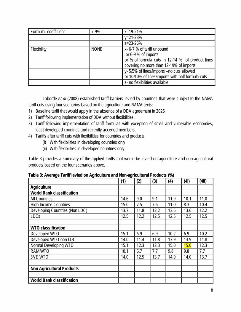
Formula- coefficient 7-9% x=19-21% y=21-23% z=23-26% Flexibility NONE x- 6-7 % of tariff unbound

or 6-9 % of imports or ½ of formula cuts in 12-14 % of product lines covering no more than 12-19% of imports

y- 5/5% of lines/imports –no cuts allowed or 10/10% of lines/imports with half formula cuts

z- no flexibilities available

Laborde et al (2008) established tariff barriers levied by countries that were subject to the NAMA tariff cuts using four scenarios based on the agriculture and NAMA texts: 1) Baseline tariff that would apply in the absence of a DDA agreement in 2025 2) Tariff following implementation of DDA without flexibilities. 3) Tariff following implementation of tariff formulas with exception of small and vulnerable economies,

least developed countries and recently acceded members. 4) Tariffs after tariff cuts with flexibilities for countries and products

(i) With flexibilities in developing countries only (ii) With flexibilities in developed countries only.

Table 3 provides a summary of the applied tariffs that would be levied on agriculture and non-agricultural products based on the four scenarios above.

Table 3: Average Tariff levied on Agriculture and Non-agricultural Products (%) (1) (2) (3) (4) (4i) (4ii) Agriculture World Bank classification All Countries 14.6 9.0 9.1 11.9 10.1 11.0 High Income Countries 15.0 7.5 7.6 11.0 8.3 10.4 Developing Countries (Non LDC) 13.7 11.8 12.2 13.6 13.6 12.2 LDCs 12.5 12.2 12.5 12.5 12.5 12.5 WTO classification Developed WTO 15.1 6.9 6.9 10.2 6.9 10.2 Developed WTO non LDC 14.0 11.4 11.8 13.9 13.9 11.8 Normal Developing WTO 15.1 12.3 12.3 15.0 15.0 12.3 RAM WTO 10.1 6.7 7.7 9.8 9.8 7.7 SVE WTO 14.0 12.5 13.7 14.0 14.0 13.7 Non Agricultural Products World Bank classification

9

(1) (2) (3) (4) (4i) (4ii) All Countries 2.9 2.1 2.2 2.3 2.3 2.2 High Income Countries 1.7 1.1 1.1 1.1 1.1 1.1 Developing Countries (Non LDC) 6.4 4.8 5.3 5.6 5.6 5.1 LDCs 10.9 8.0 10.9 10.9 10.9 10.9 WTO classification Developed WTO 1.7 1.0 1.0 1.0 1.0 1.0 Developed WTO non LDC 4.8 3.7 4.0 4.3 4.3 3.9 Normal Developing WTO 3.9 3.1 3.1 3.4 3.4 3.0 RAM WTO 4.9 3.5 3.5 3.9 3.9 3.5 SVE WTO 8.9 6.7 8.9 8.9 8.9 8.9

Source: Laborde et al (2008)

The above changes in tariff levels particularly for developing countries as per the WTO classification will provide the basis for the tariff reduction scenarios to undertake. For the analysis scenario 4(i) will be the most appropriate as tariff reduction will be accompanied by flexibilities. Based on the applied tariffs estimated by Laborde et al (ibid), the current applied tariffs for agriculture and NAMA products for Kenya were compared against their estimations and the amount by which applied tariffs would reduce/increased were then established to be used for the simulations. Two scenarios will be used to undertake simulations: 1) Trade liberalization scenario where average applied tariffs for agricultural products reduce by 0.71

percent and average applied tariff for NAMA products reduce by 10.42 percent. While considering special/sensitive products

2) Full liberalization where all tariffs are eliminated including sensitive products.

10

3 METHODOLOGICAL FRAMEWORK

3.1 INTERNATIONAL TRADE THEORY- THE NEOCLASSICAL THEORY The methodological framework to be used for examining the impact of trade liberalization on

poverty is based on the neoclassical theory of trade. The neoclassical school of economic thought was predominant in the 19th century especially in the United States and it differs from the ‘classical’ economic thought hence the prefix ‘neo’. The foundations of the neoclassical model of international trade were laid by Eli Hecksher and his pupil Bertil Ohlin (1899-1979) a Swedish economist. Neoclassical economics has remained the dominant school of thought; it relates supply and demand to an individual’s rationality and his/her ability to maximize utility or profits. The Neoclassical theory of trade consists of four theorems: the Hecksher-Ohlin (H-O) theorem, the Rybczynski theorem, the Stolper-Samuelson theorem and the factor price equalization theory.

The H-O model, argues that the pattern of international trade is determined by differences in factor endowments argues that with free trade, the aggregate welfare of a country will be raised relative to the welfare under autarky. The Rybczynski theorem provides the link between production level of final goods and the available factors of production. It demonstrates how changes in endowments affect the output of goods when full employment is maintained. It predicts that countries will export those goods that make intensive use of locally abundant factors and will import goods that make intensive use of factors that are locally scarce. It states that: “With two final goods, two factors of production and constant prices of the final goods, an increase in the supply of the factors of production results in an increase of the output of the final good that uses this factor of production relatively intensively and a reduction in the output of the other final good, provided both goods are produced in equilibrium”

The Stolper-Samuelson proposition was derived by Wolfgang Stolper and Paul Samuelson. This proposition provides the impact of a change in the price of the final good to the rewards of the factors of production and the factor intensity of the production process. It states that: “With two final goods and two factors of production, an increase in the price of final good increases the reward to the factors of production used intensively in the production of that good and reduces the reward to other factors provided that both good are produced.” The Factor Price Equalization (FPE) forms the cornerstone of the neoclassical framework and also the most fragile of the theories. FPE as postulated by Bertil Ohlin state that: “Free trade in commodities will eliminate price differentials, thereby effecting equalization of factor prices; especially wages and interest rates, so that when the prices of the output goods are equalized between countries as free trade occurs, then the prices of the factors (capital and labour) will also be equalized between countries. These theorems form the foundation of the neoclassical theory of trade and are the cornerstones of arguments in favour of trade liberalization.

3.2 THE CGE MODEL The research adopts the IFPRI computable general equilibrium model following the work of Lofgren

et al (2002). The CGE model is Walrasian in nature since it assumes the product and factor markets clear and prices adjust in these markets in order to achieve equilibrium. The concept of economic equilibrium

11

was first brought to the fore by Leon Walras (1874), he highlighted the interrelationships between markets where supply and demand of different commodities are met under perfect competition, commodity prices match the cost of production hence equilibrium is achieved. Walrasian equilibrium was further applied by Arrow and Debreu (1954) and Debreu (1959) to real economies. Subsequently other authors have used these models for different economic issues, for example, Chenery and Uzawa (1958) used the CGE model to analyze economic development, Harberger (1962) examined issues of taxation, while more recent studies by Lofgren et al (2002), Sherman (2006) have examined the impact of trade liberalization on different aspects of the economy.

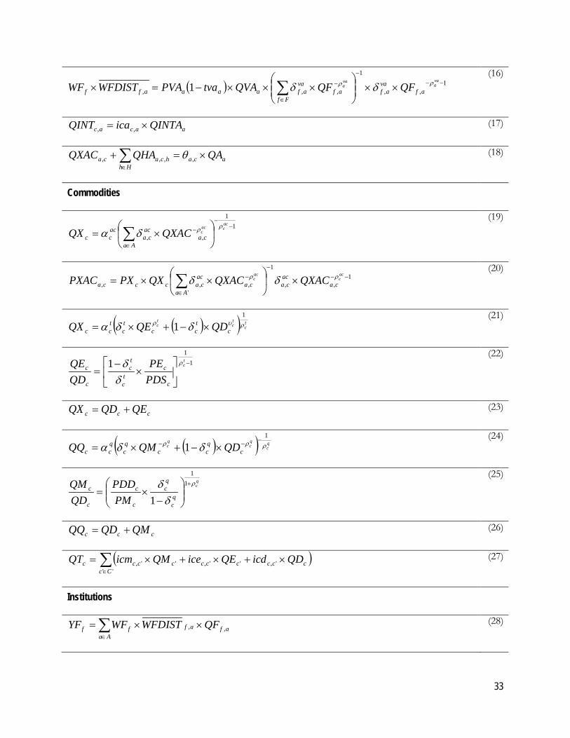
The CGE model as illustrated by Lofgren et al (2002) has the price and production blocks which incorporates production, distribution and demand. Equilibrium in these markets is determined by wages and prices adjusting simultaneously in all markets. Equations (1) to (10) in the appendix 1 indicate the prices derived from the model, they are in relative terms, any absolute prices required are determined exogenously. Producers maximize their profits depending on the level of technology and aggregated factor supply i.e. labour and capital. Production is assumed to take place in two stages: in the first stage, value added and intermediate consumption is combined using Leontief technology and in the second stage, different factors: capital land and labour are combined using constant elasticity of substitution (CES) technology to produce value added, while different intermediate inputs are also combined to produce intermediate consumption. Equations (11) to (18) indicate the equations of the production block of the CGE model. Equations (19) to (27) provides the equations for the commodity block showing aggregate output produced by combining activities of different commodities. Aggregate output is then composed of aggregates exports and domestic production. Based on the work of Armington (1969), who introduced imperfect substitutability of goods which has largely been extended to the trade sector, there is imperfect substitution between imported and domestically produced goods, so that import demand is based on constant elasticity of substitution while export supply is based on constant elasticity of transformation. Domestically produced goods combined with imports produce a composite commodity which is consumed by households, government, intermediate use and investment. The institutions incorporated in this model are households, government, enterprises and the rest of the world. These institutions provide a path through which trade liberalization affects households. Equations (28) to (32) provide incomes of institutions including intra institutional transfers. Equations (33) and (34) are the consumption of marketed and home produced commodities by households. The model closure of the IFPRI model is illustrated by Lofgren et al (2002) and Robinson (2003). Given the assumption of the fixed supply of primary factors of production, equilibrium in these markets is determined by wages and prices adjusting simultaneously in all markets so that supply equals demands in both factor and product markets. Supply and demand equations are also homogeneous of degree zero in prices so that doubling prices does not change demand. The trade balance i.e. foreign savings is assumed to be fixed, real exchange rate adjusts to achieve equilibrium, hence with fixed foreign savings, investment is said to be ‘savings driven’. Government revenue must equal expenditure while total savings must equal total investment. This CGE model is the orthodox applied neoclassical model for welfare analysis. However, there are other strands of CGE models that do relax the Walrasian restrictions so that new elements such as nominal price rigidities, unbalanced government budgets in equilibrium and nominal exchange rates are introduced. Johansen

12

(1960) pioneered such works followed by macro structuralists as Lance Taylor (1990) whose works are more focused on Keynesian economics.

3.3 DATA The social accounting matrix for Kenya 2003 was used in this analysis. The Kenyan SAM has 50 commodity/activity accounts. The activity account is valued at producers’ prices, in this case Kshs. 1,886,249 million. The commodity account is valued at purchase prices i.e. Kshs. 2,440,000 million, which includes indirect commodity taxes and transaction costs. There are two factors of production in this matrix: labour (Kshs. 430,332 million) and capital (Kshs. 499,236 million). Labour has been further subdivided into skilled, semi-skilled and unskilled, while capital includes land. Trade and transportation costs are the costs associated with domestic, import, and export marketing are valued at Kshs. 97,623 million. Government income and payments are disaggregated into a core government account and different tax collection accounts are valued at Kshs. 218,359 million. The households in the SAM consist of both urban and rural and are divided into ten so that there are 20 households in total. The capital account has the saving-investment account valued at Kshs. 196,554 million and the change in stock account values at Kshs. 17,444 million. The rest of the world account which deals with imports and exports are valued at Kshs. 424,120 million.

13

4 SIMULATION RESULTS AND DISCUSSION Two simulations were undertaken; Trade liberalization scenario where average tariffs for agricultural products reduce by 0.71 percent and average applied tariff for NAMA products reduce by 10.42 percent. While considering special/sensitive products and full liberalization where all tariffs are eliminated. Lastly a dynamic simulation was provided to establish the trade outlook of Kenya in 15 years’ time.

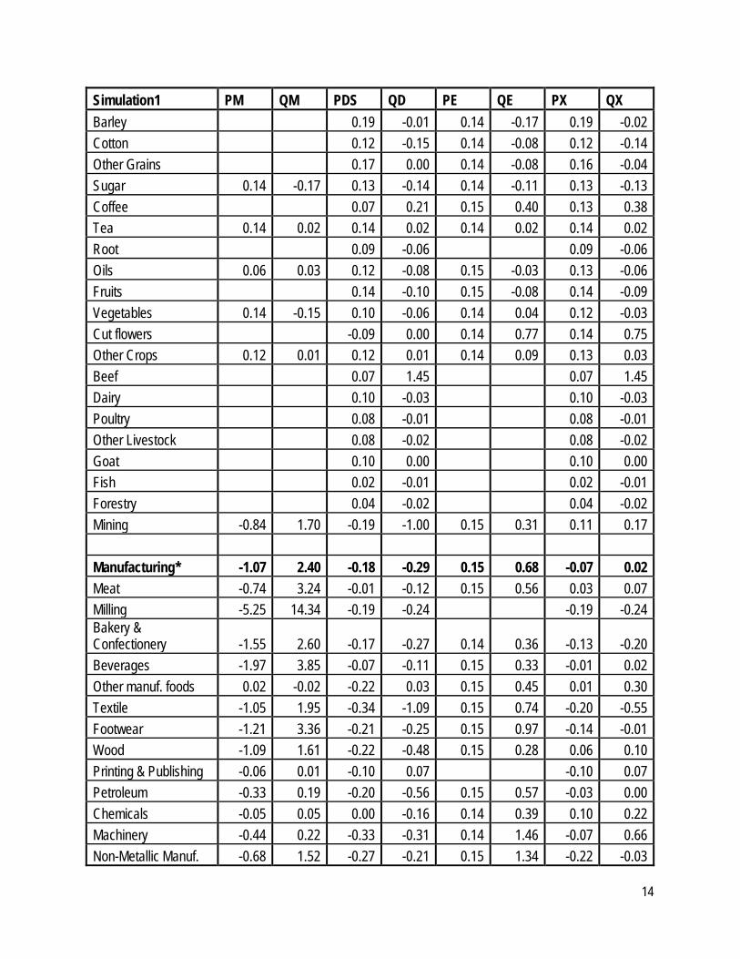
4.1 PRICE AND VOLUME EFFECTS Table 9 provides a summary of the sectoral impacts of trade liberalization. Under Simulation 1

most agricultural commodities are protected as special /sensitive products therefore a 0.02 percent increase in import prices leads to a 0.11 percent increase in quantity demanded of agricultural imports. The manufacturing sector recorded an import price decrease of 1.07 percent resulting in a 2.4 percent increase in the quantity of manufactured. Services were not part of the simulations, however, prices changes were due to exchange rates and indirect effects associated with increases in import demand of commodities with strong links to services. Domestic sales on the other hand adjust to the changes of import prices and quantities. Given the price increase in agricultural imports, the prices of domestic supply of agricultural commodities increase by 0.08 percent resulting in a 0.01 percent decrease in quantity demanded. Specific agricultural commodities are not much affected in this simulation since most of them are protected and are not subject to tariff cuts, while at the same time, considering that the tariff reduction was 0.72 percent. For manufactured products, the domestic supply price of decrease by 0.18 percent resulting in a 0.29 percent decrease in quantity demanded. Normally when imports increase, exports prices should increase in order to maintain the same level of balance of payment and also because producers switching to export production. The increase in export prices on the other hand can also be attributed to exchange rate increases as also found by Sharma (2008) on similar studies done in India. From table 9, the price of agricultural exports has increased by 0.14 percent leading to an increase in quantity exported by 0.07 percent. This increase can be attributed to exchange rate adjustments. The changes in prices and volumes for different agricultural and non- agricultural commodities are also provided. Specific manufactured commodities that are affected by the tariff reductions include milling, beverages and bakery and confectionery (5.25, 1.97 and 1.55 percent respectively) resulting in increase in imported quantities (14.34, 3.85 and 3.24 respectively)

Table 4: Effects of Trade Liberalization on Sectoral Prices and Volumes. Simulation1 PM QM PDS QD PE QE PX QX

Agriculture* 0.02 0.11 0.08 -0.01 0.14 0.07 0.11 0.08 Maize 0.14 -0.22 0.09 -0.06 0.14 0.10 0.09 -0.06 Wheat 0.14 -0.16 0.15 -0.17 0.14 -0.18 0.15 -0.17 Rice 0.14 -0.10 0.08 -0.03 0.08 -0.03

14

Simulation1 PM QM PDS QD PE QE PX QX Barley

0.19 -0.01 0.14 -0.17 0.19 -0.02

Cotton

0.12 -0.15 0.14 -0.08 0.12 -0.14 Other Grains

0.17 0.00 0.14 -0.08 0.16 -0.04

Sugar 0.14 -0.17 0.13 -0.14 0.14 -0.11 0.13 -0.13 Coffee

0.07 0.21 0.15 0.40 0.13 0.38

Tea 0.14 0.02 0.14 0.02 0.14 0.02 0.14 0.02 Root

0.09 -0.06 0.09 -0.06

Oils 0.06 0.03 0.12 -0.08 0.15 -0.03 0.13 -0.06 Fruits

0.14 -0.10 0.15 -0.08 0.14 -0.09

Vegetables 0.14 -0.15 0.10 -0.06 0.14 0.04 0.12 -0.03 Cut flowers

-0.09 0.00 0.14 0.77 0.14 0.75

Other Crops 0.12 0.01 0.12 0.01 0.14 0.09 0.13 0.03 Beef

0.07 1.45 0.07 1.45

Dairy

0.10 -0.03 0.10 -0.03 Poultry

0.08 -0.01 0.08 -0.01

Other Livestock

0.08 -0.02 0.08 -0.02 Goat

0.10 0.00 0.10 0.00

Fish

0.02 -0.01 0.02 -0.01 Forestry

0.04 -0.02 0.04 -0.02

Mining -0.84 1.70 -0.19 -1.00 0.15 0.31 0.11 0.17

Manufacturing* -1.07 2.40 -0.18 -0.29 0.15 0.68 -0.07 0.02 Meat -0.74 3.24 -0.01 -0.12 0.15 0.56 0.03 0.07 Milling -5.25 14.34 -0.19 -0.24 -0.19 -0.24 Bakery & Confectionery -1.55 2.60 -0.17 -0.27 0.14 0.36 -0.13 -0.20 Beverages -1.97 3.85 -0.07 -0.11 0.15 0.33 -0.01 0.02 Other manuf. foods 0.02 -0.02 -0.22 0.03 0.15 0.45 0.01 0.30 Textile -1.05 1.95 -0.34 -1.09 0.15 0.74 -0.20 -0.55 Footwear -1.21 3.36 -0.21 -0.25 0.15 0.97 -0.14 -0.01 Wood -1.09 1.61 -0.22 -0.48 0.15 0.28 0.06 0.10 Printing & Publishing -0.06 0.01 -0.10 0.07 -0.10 0.07 Petroleum -0.33 0.19 -0.20 -0.56 0.15 0.57 -0.03 0.00 Chemicals -0.05 0.05 0.00 -0.16 0.14 0.39 0.10 0.22 Machinery -0.44 0.22 -0.33 -0.31 0.14 1.46 -0.07 0.66 Non-Metallic Manuf. -0.68 1.52 -0.27 -0.21 0.15 1.34 -0.22 -0.03

15

Simulation1 PM QM PDS QD PE QE PX QX Other manufactures -0.63 0.70 -0.24 -0.41 0.14 0.66 -0.15 -0.17

Services* 0.14 -0.15 0.03 0.56 0.14 0.13 0.03 0.57

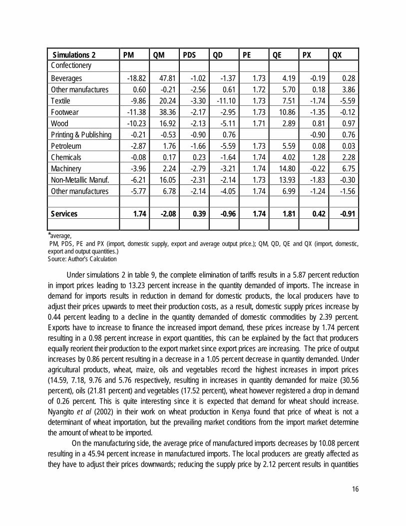
Simulations 2 PM QM PDS QD PE QE PX QX Agriculture -5.87 13.23 0.44 -2.39 1.74 0.98 0.86 -1.05 Maize -7.18 30.56 1.03 -1.36 1.74 0.95 1.03 -1.34 Wheat -14.59 -0.26 -6.44 -26.61 1.74 -3.23 -5.10 -23.08 Rice 1.74 -1.44 0.89 -0.59 0.89 -0.59 Barley 2.13 0.01 1.74 -1.23 2.09 -0.12 Cotton 1.38 -1.40 1.74 -0.26 1.41 -1.31 Other Grains 1.88 -0.01 1.74 -0.48 1.82 -0.20 Sugar -2.09 1.20 0.63 -3.86 1.74 -1.89 1.00 -3.20 Coffee 0.73 2.66 1.73 5.18 1.60 4.85 Tea -5.84 23.50 0.83 -1.35 1.73 1.55 1.66 1.29 Root 0.92 -0.85 0.92 -0.85 Oils -9.76 21.81 1.15 -1.48 1.73 -0.43 1.37 -1.09 Fruits 1.50 -1.21 1.73 -0.48 1.54 -1.08 Vegetables -5.76 17.52 0.96 -1.23 1.73 0.67 1.20 -0.65 Cut flowers -0.89 0.00 1.74 8.88 1.70 8.74 Other Crops -1.59 8.71 1.12 -0.47 1.74 1.54 1.31 0.13 Beef 0.69 -6.09 0.69 -6.09 Dairy 0.93 -0.31 0.93 -0.31 Poultry 0.56 -0.11 0.56 -0.11 Other Livestock 0.69 -0.27 0.69 -0.27 Goat 1.05 -0.05 1.05 -0.05 Fish -0.09 -0.12 -0.09 -0.12 Forestry 0.16 -0.29 0.16 -0.29 Mining -7.77 17.51 -1.77 -9.99 1.73 2.99 1.37 1.62 Manufacturing -10.08 45.94 -2.12 -3.09 1.73 7.46 -0.93 0.23 Meat Processing -6.79 34.87 -0.22 -1.45 1.73 7.28 0.32 0.90 Milling -50.79 429.75 -6.39 -3.47 -6.39 -3.47 Bakery & -14.69 28.92 -2.31 -2.49 1.73 5.75 -1.86 -1.60

16

Simulations 2 PM QM PDS QD PE QE PX QX Confectionery Beverages -18.82 47.81 -1.02 -1.37 1.73 4.19 -0.19 0.28 Other manufactures 0.60 -0.21 -2.56 0.61 1.72 5.70 0.18 3.86 Textile -9.86 20.24 -3.30 -11.10 1.73 7.51 -1.74 -5.59 Footwear -11.38 38.36 -2.17 -2.95 1.73 10.86 -1.35 -0.12 Wood -10.23 16.92 -2.13 -5.11 1.71 2.89 0.81 0.97 Printing & Publishing -0.21 -0.53 -0.90 0.76 -0.90 0.76 Petroleum -2.87 1.76 -1.66 -5.59 1.73 5.59 0.08 0.03 Chemicals -0.08 0.17 0.23 -1.64 1.74 4.02 1.28 2.28 Machinery -3.96 2.24 -2.79 -3.21 1.74 14.80 -0.22 6.75 Non-Metallic Manuf. -6.21 16.05 -2.31 -2.14 1.73 13.93 -1.83 -0.30 Other manufactures -5.77 6.78 -2.14 -4.05 1.74 6.99 -1.24 -1.56 Services 1.74 -2.08 0.39 -0.96 1.74 1.81 0.42 -0.91

*average, PM, PDS, PE and PX (import, domestic supply, export and average output price.); QM, QD, QE and QX (import, domestic, export and output quantities.) Source: Author’s Calculation

Under simulations 2 in table 9, the complete elimination of tariffs results in a 5.87 percent reduction in import prices leading to 13.23 percent increase in the quantity demanded of imports. The increase in demand for imports results in reduction in demand for domestic products, the local producers have to adjust their prices upwards to meet their production costs, as a result, domestic supply prices increase by 0.44 percent leading to a decline in the quantity demanded of domestic commodities by 2.39 percent. Exports have to increase to finance the increased import demand, these prices increase by 1.74 percent resulting in a 0.98 percent increase in export quantities, this can be explained by the fact that producers equally reorient their production to the export market since export prices are increasing. The price of output increases by 0.86 percent resulting in a decrease in a 1.05 percent decrease in quantity demanded. Under agricultural products, wheat, maize, oils and vegetables record the highest increases in import prices (14.59, 7.18, 9.76 and 5.76 respectively, resulting in increases in quantity demanded for maize (30.56 percent), oils (21.81 percent) and vegetables (17.52 percent), wheat however registered a drop in demand of 0.26 percent. This is quite interesting since it is expected that demand for wheat should increase. Nyangito et al (2002) in their work on wheat production in Kenya found that price of wheat is not a determinant of wheat importation, but the prevailing market conditions from the import market determine the amount of wheat to be imported. On the manufacturing side, the average price of manufactured imports decreases by 10.08 percent resulting in a 45.94 percent increase in manufactured imports. The local producers are greatly affected as they have to adjust their prices downwards; reducing the supply price by 2.12 percent results in quantities

17

demanded decreasing by 3.09 percent. Export prices equally adjust upwards by 1.73 percent resulting in increase in exports by 7.46 percent. These adjustments decrease overall manufacturing output by 0.23 percent. The main manufacturing products affected are milling, beverages, and bakers and confectionery which record major decreases in their import prices (50.79, 18.82 and 14.69 percent respectively) resulting in increase in quantities demanded (429.75, 47.81 and 28.92 percent respectively). Clearly, the manufacturing sector has gained more from trade liberalization; this can be attributed to the fact that our import concentration index is approximately 52 percent.

4.2 FACTOR MOVEMENT AND VALUE ADDED The impact of trade liberalization will result in reallocation of resources and sectors are therefore

affected differently. The change in sectoral price and volumes as shown on table 9 will also result in changes in factor demand and the quantity demanded of factors of production which also affects the quantity of value added. Factor demand has a direct effect on welfare since incomes will be affected. Under simulation 1, the demand for all categories of labour (skilled, semi-skilled and unskilled) has increased for agriculture while the demand for land decreases by 0.025 percent. As a result the quantity of value added has also increased by 0.011 percent. Since most agricultural commodities are protected in this simulation, changes in factor demand are quite small. In the manufacturing sector, demand for skilled labour reduces by 0.046 percent while semi-skilled and unskilled labour demand increase by 0.012 and 0.014 percent respectively. Overall demand for value added has increased by 0.023 percent. The demand for value added for milling, bakery and confectionery, textiles, footwear, non-metallic manufactures and other manufactures. The demand for value added equally decreases for the services sector due to liberalization. Table 5: Change in Factor Demand and Value Added by Sectors (%) Simulation 1 Skilled Semi-Skilled Unskilled QVA Agriculture* 0.005 0.040 0.056 0.011 Maize -0.071 -0.037 -0.025 -0.062 Wheat -0.186 -0.152

-0.166

Rice -0.034 0.000

-0.034 Barley -0.006 0.028

-0.023

Cotton -0.149 -0.115 -0.104 -0.143 Other Grains -0.030 0.004 0.016 -0.036 Sugar -0.138 -0.104 -0.092 -0.130 Coffee 0.440 0.475 0.486 0.375 Tea 0.019 0.053 0.065 0.018 Roots & Tubers -0.099 -0.065 -0.054 -0.063 Oils -0.083 -0.049 -0.037 -0.078 Fruits -0.115 -0.080 -0.069 -0.110 Vegetables -0.073 -0.038 -0.027 -0.046

18

Simulation 1 Skilled Semi-Skilled Unskilled QVA Cut Flowers 0.852 0.886 0.898 0.753 Other Crops 0.043 0.077 0.088 0.034 Beef -0.023 0.011 0.022

-0.002

Dairy -0.108 -0.074 -0.063

-0.055 Poultry -0.089 -0.054 -0.043

-0.038

Goat -0.086 -0.051 -0.040

-0.043 Other Livestock -0.114 -0.080 -0.069

-0.036

Fish -0.059 -0.025

-0.004 Forestry -0.094 -0.060

-0.017

Mining 0.329 0.363

0.166

Manufacturing* -0.046 0.012 0.040

0.023 Meat 0.182 0.216 0.227

0.065

Milling -1.121 -1.087 -1.076

-0.159 Bakery & Confectionery -0.384 -0.350 -0.338

-0.199

Beverage

0.047 0.058

0.020 Other Manufactures 0.641 0.675 0.687

0.300

Textile -0.829 -0.796 -0.784

-0.552 Footwear -0.039 -0.005

-0.005

Wood 0.212 0.246 0.258

0.097 Print

0.162

0.073

Petroleum

0.096 0.108

0.002 Chemicals 0.390 0.424 0.436

0.216

Machinery 1.060 1.095 1.106

0.663 Non-metallic Manuf. -0.339 -0.305

-0.032

Other Manufactures -0.283 -0.249 -0.238

-0.170

Services* -0.036 -0.016 -0.004

-0.009

Simulation 2 Skilled Semi-Skilled Unskilled QVA Agriculture* -1.158 -0.748 0.646 -0.810 Maize -1.505 -1.097 -0.835 -1.280 Wheat -25.993 -25.686

-21.609

Rice -0.705 -0.293

-0.595 Barley 0.008 0.423

-0.124

Cotton -1.410 -1.001 -0.739 -1.312 Other Grains -0.153 0.261 0.526 -0.204 Sugar -3.569 -3.169 -2.913 -3.198

19

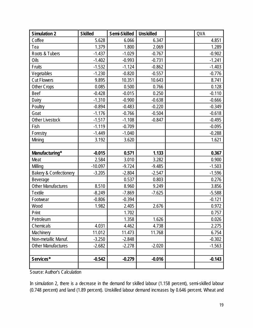
Simulation 2 Skilled Semi-Skilled Unskilled QVA Coffee 5.628 6.066 6.347 4.851 Tea 1.379 1.800 2.069 1.289 Roots & Tubers -1.437 -1.029 -0.767 -0.902 Oils -1.402 -0.993 -0.731 -1.241 Fruits -1.532 -1.124 -0.862 -1.403 Vegetables -1.230 -0.820 -0.557 -0.776 Cut Flowers 9.895 10.351 10.643 8.741 Other Crops 0.085 0.500 0.766 0.128 Beef -0.428 -0.015 0.250 -0.110 Dairy -1.310 -0.900 -0.638

-0.666

Poultry -0.894 -0.483 -0.220

-0.349 Goat -1.176 -0.766 -0.504

-0.618

Other Livestock -1.517 -1.108 -0.847

-0.495 Fish -1.119 -0.709

-0.095

Forestry -1.449 -1.040

-0.288 Mining 3.192 3.620

1.621

Manufacturing* -0.015 0.571 1.133

0.367 Meat 2.584 3.010 3.282

0.900

Milling -10.097 -9.724 -9.485

-1.503 Bakery & Confectionery -3.205 -2.804 -2.547

-1.596

Beverage

0.537 0.803

0.276 Other Manufactures 8.510 8.960 9.249

3.856

Textile -8.249 -7.869 -7.625

-5.588 Footwear -0.806 -0.394

-0.121

Wood 1.982 2.405 2.676

0.972 Print

1.702

0.757

Petroleum

1.358 1.626

0.026 Chemicals 4.031 4.462 4.738

2.275

Machinery 11.012 11.473 11.768

6.754 Non-metallic Manuf. -3.250 -2.848

-0.302

Other Manufactures -2.682 -2.278 -2.020

-1.563

Services* -0.542 -0.279 -0.016

-0.143

Source: Author’s Calculation

In simulation 2, there is a decrease in the demand for skilled labour (1.158 percent), semi-skilled labour (0.748 percent) and land (1.89 percent). Unskilled labour demand increases by 0.646 percent. Wheat and

20

sugar record the highest reduction in the quantity of value added while cut flowers gains the most in the increase for demand for quantity of value added. In the manufacturing sector, the demand for skilled labour decreases by 0.015 percent while semi-skilled and unskilled labour increase by 0.6 and 1.1 percent respectively. With full liberalization the demand for labour is greatly reduces in milling, bakery and confectionery and textiles, at the same time, other manufactures, and machinery record a leap in demand for all labour categories. Labour demand is negatively affected in the services sector.

4.3 CONSUMPTION EFFECTS The changes in sectoral prices and volume due to trade liberalization equally affect the incomes

which in turn affect household consumption. The changes in household consumption are shown on table 11. The households are divided into deciles hence there are twenty households in total. In simulation 1, there is minimal change in real household consumption which is 0.10 percent for most rural households In the urban households, the poorest household, urban1, 3 and 7 record a 0.10 percent increase in real consumption while rural7-10 and Urban0, 5, 6, 8 and 9 do not record any increases in real consumption. With full liberalization, most the urban households 0, 2 and 4 record approximately 2 percent increase in real consumption. Table 6: Changes in Households Real Consumption (%)

Simulation 1 Simulation 2 Simulation 1 Simulation 2

Rural0 0.10 1.60 Urban0 2.70 Rural1 0.10 1.40 Urban1 0.10 1.40 Rural2 0.10 1.00 Urban2 0.20 2.10 Rural3 0.10 1.00 Urban3 0.10 1.80 Rural4 0.10 0.80 Urban4 0.20 2.00 Rural5 0.10 0.70 Urban5 -0.10 Rural6 0.10 0.70 Urban6 0.60 Rural7

0.50 Urban7 0.10 0.90

Rural8

0.50 Urban8 -0.30 Rural9

0.20 Urban9 0.10

Source: Author’s Calculation

4.4 WELFARE EFFECTS The measure of welfare in this analysis is equivalent variation (EV), changes in nominal income and consumer price index (CPI). Table 12 provides the changes in welfare based on the three indicators. Under simulation 1, there is a 0.1 percent increase in equivalent variation for rural households 1-6. Rural7 to 9 do not have any increase in equivalent variations, the EV therefore shows that consumption has increased for

21

rural households as compared to the urban households. Column 2 provides the percentage change in nominal incomes; rural0 has the highest percentage change in nominal incomes. Comparing to urban households under simulation 1, urban4 has the highest increase in equivalent variation compared to the other urban households. Furthermore, while all urban households have increases in nominal income, urban0, which is the poorest urban decile, records a 0.006 percent decrease in income. All urban households have a decrease in the price index particularly the poor households. Table 7: Welfare Impacts (%) Simulation 1 Simulation 2 EV Income CPI Change EV Income CPI Change Rural0 0.1 0.187 0.000 1.6 2.045 -0.781 Rural1 0.1 0.166 0.000 1.4 1.793 -0.773 Rural2 0.1 0.146 -0.110 1 1.554 -0.661 Rural3 0.1 0.14 -0.110 1 1.499 -0.661 Rural4 0.1 0.13 -0.110 0.8 1.36 -0.661 Rural5 0.1 0.129 0.000 0.7 1.344 -0.550 Rural6 0.1 0.126 0.000 0.7 1.301 -0.552 Rural7 0.118 -0.111 0.5 1.217 -0.556 Rural8 0.12 0.000 0.5 1.229 -0.559 Rural9 0.1 0.000 0.2 0.976 -0.452 Urban0 -0.006 -0.249 2.6 -0.318 -5.603 Urban1 0.1 0.098 -0.127 1.3 1.049 -1.906 Urban2 0.1 0.137 -0.250 2.1 1.49 -2.243 Urban3 0.1 0.165 -0.120 1.8 1.862 -1.435 Urban4 0.2 0.162 -0.125 2 1.822 -1.743 Urban5 0.054 0.000 -0.2 0.446 -0.716 Urban6 0.046 -0.249 0.5 0.356 -1.616 Urban7 0.1 0.085 -0.121 0.8 0.86 -1.573 Urban8 0.047 0.000 -0.3 0.325 -0.706 Urban9 0.087 0.000 0.806 -0.588

Source: Author’s Calculation

Simulation 2 provides higher changes in equivalent variation compared to simulation 1 for all rural households, however, in the urban households Urban5 and 10 record a decrease in equivalent variation. The change in CPI for urban households is much higher than that of rural households, while comparing the changes in nominal income; Urban0 has a decrease in income. In general, rural households have registered a higher percentage change in income compared to urban households.

22

4.5 POVERTY The measure of welfare in this analysis is equivalent variation (EV), changes in nominal income and

consumer price index (CPI). Table 2 provides the changes in welfare based on the three indicators. Under simulation 1, nominal incomes have increased for all households, the price index has also reduced for most households and there is a 0.1 percent increase in equivalent variation for rural households except the richest decile, while in the urban households, deciles 5, 8 and 9 do not have any increases in EV implying increases in consumption. The results in simulation 2 show similar trend with higher magnitudes. These indicators are important in establishing whether welfare has improved. Table 2: Welfare Impacts (%)

Sim1

Sim2

Change in nominal income (%)

Change in CPI (%)

Equivalent Variation

Change in nominal income (%)

Change in CPI (%)

Equivalent Variation

Rural0 0.151 0.000 0.1 1.789 -0.781 1.5 Rural1 0.139 0.000 0.1 1.606 -0.773 1.3 Rural2 0.128 -0.110 0.1 1.425 -0.661 1.0 Rural3 0.125 -0.110 0.1 1.389 -0.661 1.0 Rural4 0.113 -0.110 0.1 1.234 -0.661 0.8 Rural5 0.114 0.000 0.1 1.231 -0.550 0.7 Rural6 0.113 0.000 0.1 1.198 -0.552 0.7 Rural7 0.111 -0.111 0.1 1.162 -0.556 0.6 Rural8 0.111 0.000 0.1 1.162 -0.559 0.5 Rural9 0.094 0.000 0.0 0.926 -0.452 0.2 Urban0 0.000 -0.249 0.1 -0.235 -5.603 2.0 Urban1 0.107 -0.127 0.1 1.112 -1.906 1.4 Urban2 0.125 -0.250 0.1 1.389 -2.243 2.0 Urban3 0.155 -0.120 0.1 1.711 -1.435 1.7 Urban4 0.154 -0.125 0.1 1.728 -1.743 1.9 Urban5 0.056 0.000 0.0 0.472 -0.716 -0.2 Urban6 0.052 -0.249 0.1 0.418 -1.616 0.5 Urban7 0.091 -0.121 0.1 0.905 -1.573 0.8 Urban8 0.047 0.000 0.0 0.34 -0.706 -0.3 Urban9 0.087 0.000 0.0 0.81 -0.588 0.0

Source: Author’s Calculation

While the indicators in table two show that welfare has improved for most households, it would be important to establish whether these increases have led to poverty reduction, this question is answered in table 3.

The incidence of poverty using the headcount ratio has reduced by 0.07 percent under simulation 1 for the rural households while in the urban households the increase is by approximately 1 percent. The income gap (P1), has also reduced in both simulations, however, there magnitude of change is higher in the urban areas as compared to the rural areas. In terms of poverty severity, the changes in both scenarios are not different form each other.

23

Table 3: Poverty Incidence (%)

Head Change in % points

Poverty Gap (%)

Change in % points Severity (%) Change in %

points Count (%) Po P1 P2 Rural Base 49.71 17.8 8.91 Simulation1 49.64 -0.07 17.77 -0.03 8.89 -0.02 Simulation2 49.11 -0.60 17.44 -0.36 8.68 -0.23 Urban Base 34.43 11.65 5.57 Simulation1 33.40 -1.03 11.64 -0.01 5.55 -0.02 Simulation2 33.38 -1.05 11.24 -0.41 5.32 -0.25

Source: Author’s Calculation

24

5 CONCLUSION AND POLICY RECOMENDATIONS In conclusion, the research has examined the impact of trade liberalization on Kenya using two

scenarios; first, tariffs are reduced for agricultural products tariffs by 0.71 percent while non - agricultural product tariffs are reduced by 10.42 percent while considering the special/sensitive products. In the second simulation, there is full elimination of tariffs on all products. Several conclusions can be reached based on the simulations undertaken. 1. In general full liberalization has a greater impact on welfare as compared to liberalization based on the

negotiations under the Doha Development Agenda, where there are minimal tariff cuts. 2. The manufacturing sector is more affected by trade liberalization as compared to the agricultural sector

with particular reference to sectoral price and volume changes. 3. The main agricultural subsectors that are affected by trade liberalization in terms of price and volume

effects are wheat, maize, sugar, tea, oils, vegetables and mining. In manufacturing, milling, bakery and confectionery, beverages, textiles, footwear and wood are greatly affected.

4. The wheat milling and textiles sub-sector are greatly affected when it comes to employment, the demand for labour will reduce in these sectors.

5. In terms of welfare loss due to trade liberalization, the urban poorest are the greatest casualties. From the analysis , it is clear that the urban poorest are the most vulnerable when it comes to

opening up the market to international trade, hence the government should put in extra efforts on initiative that would bring the urban poorest out of poverty and also ensure that they are less vulnerable to shock such as trade liberalization. While the manufacturing sector will gain more from international trade, there is bound to be a lot of shifts in demand for labour and hence employment. There should be initiatives geared towards ensuring that movement of labour between sectors is possible so that the active population is equipped with skills that will allow them to also adjust to the changing market demand for labour due to trade liberalization. The wheat, textile, milling and footwear sectors are particular vulnerable to decline in labour demand when the markets are opened up, special attention should be given to them. Lastly, the impact of trade liberalization on poverty and households welfare is positive though quite small. It could imply that trade liberalization alone is not sufficient to improve welfare but a combination of other policies that improve economic performance are also important component of ensuring that trade liberalization results in poverty reduction and development.

25

REFERENCES Armington, P., (1969). “A Theory for Demand of Products Distinguished by Place of Production.”

International Monetary Fund Staff Papers XVI. 159-178. Arrow, K., and Debreu, G., (1954). “Existence of a Competitive Equilibrium for a competitive Economy”.

Econometrica. 22(3): 265-290. Chenery, H., B., and Uzawa, H., (1958). “ Non-Linear Programming in Economic Development”. In Arrow,

K., Hurwicz, L., and Uzawa, H., (eds). Studies in Linear and non-linear Programming. Palo Alto CA; Stanford University Press.

Cicowiez, M. and A. Conconi (2008), “Linking Trade and Pro-Poor Growth: A Survey”, in Cockburn, J. and

P. Giordano (eds.), Trade and Poverty in the Developing World, Inter-American Development Bank, Washington, DC

Cloutier M., H., & Cockburn J. and Decaluwé,B.,(2008). "Education and Poverty in Vietnam: a Computable

General Equilibrium Analysis," Cahiers de recherche 0804, CIRPEE Debreu, G., (1959). Theory of Value: An Axiomatic Analysis of Economic Equilibrium. New York; Wiley. Harberger, A., (1962). “The Incidence of Corporate Income Tax.” Journal of Political Economy. 70: 215-240 Hoekman, B. “The WTO: Functions and Basic Principles” in Hoekman B., Mattoo A., and English P., (Eds)

(2002) “Development, Trade and the WTO: A handbook. World Bank: Washington D.C. Johansen, L., (1960). A Multisectoral Study of Economic Growth. Amsterdam, North Holland. Kiringai J., Thurlow J.,and Wanjala B.(2006). “A 2003 Social Accounting Matrix (SAM) For Kenya” Kenya

Institute for Public Policy Research and Analysis (KIPPRA) and International Food Policy Research Institute (IFPRI).

Laborde, D., Martin, W., and Mensbrugghe D. (2008). “ Implications of the 2008 Doha Draft Agriculture and

NAMA Market Access Modalities for Developing Countries”. http://www2.ihis.aau.dk/simulation/docs/WTO-formula-impact-Laborde-et-al-2008.pdf

Löfgren, H., Harris, B., and Robinson, S. (2002) “A Standard CGE Model in GAMs” Microcomputers in

Policy Research 5, International Food Policy Research Institute. McCulloch, N. Winters, A, L., and Cirera, X, (2000). Trade Liberalization and Poverty: A Handbook. CEPR,

London Mosley P. (1991) “Kenya” in Mosley P. Harrigan J. and Toye J. (eds.) Aid and Power: The World Bank

Policy Based Lending. Vol.II, Routledge: London.

26

Nyangito H., Ikiara M.M., and Ronge E. E., (2002). “Performance of Kenya’s Wheat Industry and Prospects for Regional Trade in Wheat Products.” KIPPRA Discussion Paper Series No. DP/17/2002.

Ongile G.A. (1998). “Gender and Agricultural Supply Responses to Structural Adjustment Programmes: A

Case Study of Small Holder Tea Producers in Kericho Kenya.” Unpublished PhD Thesis, University of Manchester.

Reinikka R. (1994). “How to Identify Trade Liberalization Episodes: An Empirical Study of Kenya.” Working

Paper Series. Centre for The Study of African Economies. WPS/94.10. Robinson S. (2003 ). "Macro Models and Multipliers: Leontief, Stone, Keynes, and CGE Models." Chapter

11, pp. 205-232, in Alain de Janvry and Ravi Kanbur, eds., Poverty, Inequality and Development: Essays in Honor of Erik Thorbecke, New York: Springer Science.

Ryan T. C. I and O’Brien F. S (2001). “Kenya country case study” in Devarajan, S. Dollar, R. D. and

Holmgren, T (eds) (2001), “Aid and Reform in Africa” World Bank, Washington D. C Swamy G. (1994). “Kenya Patchy Intermittent Commitment” in Husain I. and Faruqee R. (Eds) Adjustment

in Africa, Lessons from Country Case Studies. World Bank: Washington DC. Taylor, L.,(1990). “Structuralists CGE Models” in Taylor, L., (ed). Socially Relevant Policy Analysis:

Structural computable General Equilibrium Models for Developing World. Cambridge (MA): MIT Press, pp 1-70

Walras, L., (1874). “ Elements of Pure Economics or Theory of Social Wealth” Lausanne L. Borbax. WTO (2007), Understanding the WTO. World Trade Organization, Geneva WTO (2008a), “Revised draft modalities for agriculture”, World Trade Organization, Geneva. 19 May,

TN/AG/W/4/Rev.2 WTO (2008b), “Draft modalities for non-agricultural market access”, World Trade Organization, Geneva. 20

May, TN/MA/W/103/Rev.

27

APPENDIX

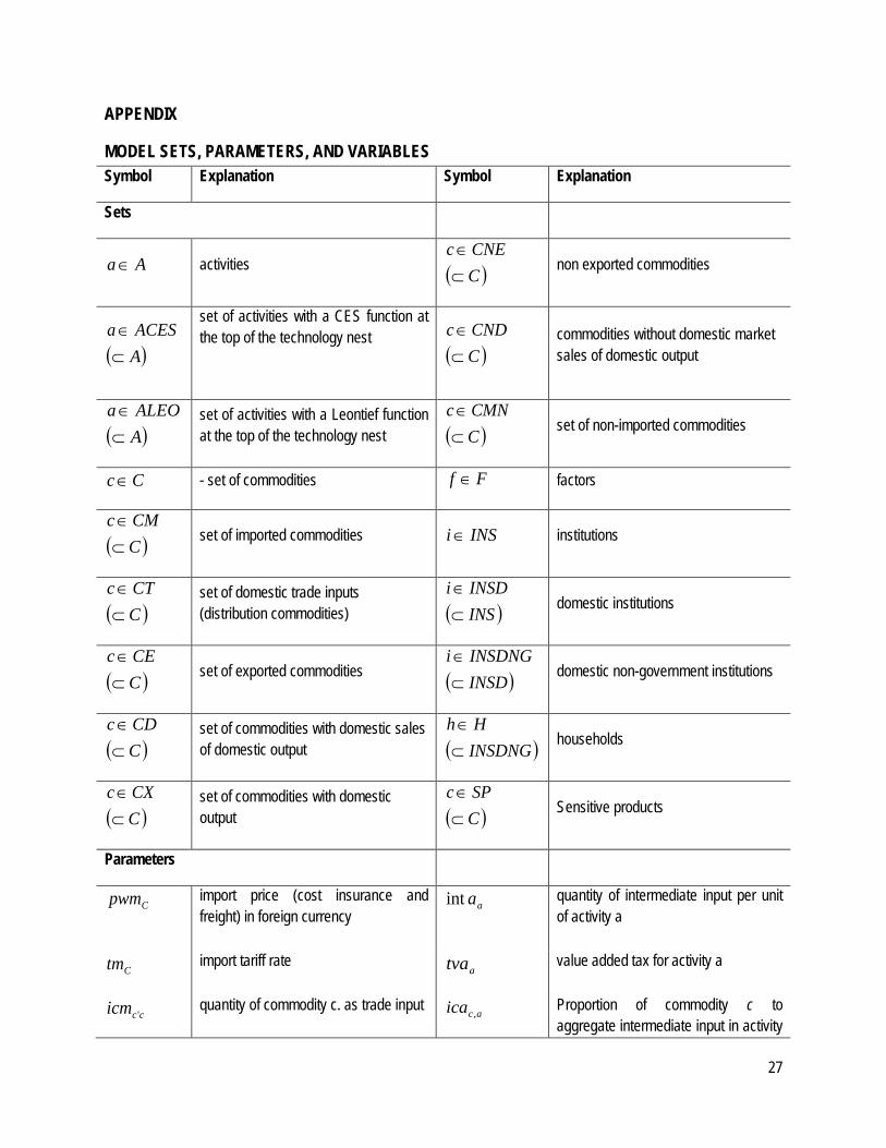
MODEL SETS, PARAMETERS, AND VARIABLES Symbol Explanation Symbol Explanation

Sets

Aa∈ activities ( )C

CNEc⊂∈

non exported commodities

( )AACESa

⊂∈

set of activities with a CES function at the top of the technology nest

( )C

CNDc⊂∈

commodities without domestic market sales of domestic output

( )AALEOa

⊂∈

set of activities with a Leontief function at the top of the technology nest ( )C

CMNc⊂∈

set of non-imported commodities

Cc∈ - set of commodities Ff ∈ factors

( )CCMc

⊂∈

set of imported commodities INSi∈ institutions

( )CCTc

⊂∈

set of domestic trade inputs (distribution commodities) ( )INS

INSDi⊂∈

domestic institutions

( )CCEc

⊂∈

set of exported commodities ( )INSD

INSDNGi⊂∈

domestic non-government institutions

( )CCDc

⊂∈

set of commodities with domestic sales of domestic output ( )INSDNG

Hh⊂∈

households

( )CCXc

⊂∈

set of commodities with domestic output ( )C

SPc⊂∈

Sensitive products

Parameters

Cpwm

import price (cost insurance and freight) in foreign currency

aaint

quantity of intermediate input per unit of activity a

Ctm import tariff rate atva value added tax for activity a

ccicm ' quantity of commodity c. as trade input acica , Proportion of commodity c to

aggregate intermediate input in activity

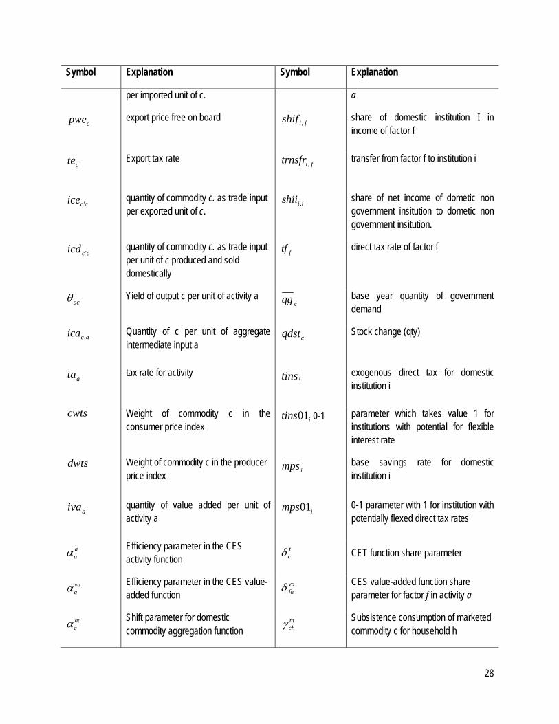
28

Symbol Explanation Symbol Explanation

per imported unit of c. a

cpwe

export price free on board fishif , share of domestic institution I in income of factor f

cte Export tax rate fitrnsfr ,

transfer from factor f to institution i

ccice '

quantity of commodity c. as trade input per exported unit of c.

iishii , share of net income of dometic non government insitution to dometic non government insitution.

ccicd ' quantity of commodity c. as trade input per unit of c produced and sold domestically

ftf direct tax rate of factor f

acθ Yield of output c per unit of activity a cqg base year quantity of government demand

acica ,

Quantity of c per unit of aggregate intermediate input a

cqdst Stock change (qty)

ata

tax rate for activity itins exogenous direct tax for domestic institution i

cwts

Weight of commodity c in the consumer price index

itins01 0-1 parameter which takes value 1 for institutions with potential for flexible interest rate

dwts

Weight of commodity c in the producer price index

imps

base savings rate for domestic institution i

aiva

quantity of value added per unit of activity a

imps01

0-1 parameter with 1 for institution with potentially flexed direct tax rates

Efficiency parameter in the CES activity function

tcδ CET function share parameter

Efficiency parameter in the CES value-added function

CES value-added function share parameter for factor f in activity a

Shift parameter for domestic commodity aggregation function

Subsistence consumption of marketed commodity c for household h

aaα

vaaα

vafaδ

accα

mchγ

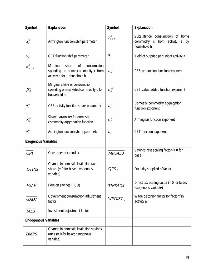
29

Symbol Explanation Symbol Explanation

Armington function shift parameter h

hca ,,γ Subsistence consumption of home commodity c from activity a by household h

CET function shift parameter Yield of output c per unit of activity a

hhca ,,β Marginal share of consumption

spending on home commodity c from activity a for household h

CES production function exponent

Marginal share of consumption spending on marketed commodity c for household h

CES value-added function exponent

CES activity function share parameter Domestic commodity aggregation function exponent

Share parameter for domestic commodity aggregation function

Armington function exponent

qcδ Armington function share parameter CET function exponent

Exogenous Variables

Consumer price index Savings rate scaling factor (= 0 for base)

Change in domestic institution tax share (= 0 for base; exogenous variable)

Quantity supplied of factor

Foreign savings (FCU) Direct tax scaling factor (= 0 for base; exogenous variable)

Government consumption adjustment factor Wage distortion factor for factor f in

activity a

Investment adjustment factor

Endogenous Variables

Change in domestic institution savings rates (= 0 for base; exogenous variable)

qcα

tcα acθ

aaρ

mchβ va

aρ

aaδ

accρ

acacδ q

cρ

tcρ

CPI MPSADJ

DTINS fQFS

FSAV TINSADJ

GADJ faWFDIST

IADJ

DMPS

30

Symbol Explanation Symbol Explanation

Producer price index for domestically marketed output

Quantity consumed of commodity c by household h

Government expenditures Quantity of household home consumption of commodity c from activity a for household h

Consumption spending for household Quantity of aggregate intermediate input

Exchange rate (LCU per unit of FCU) Quantity of commodity c as intermediate input to activity a

Government savings Quantity of investment demand for commodity

Quantity demanded of factor f from activity a cQM Quantity of imports of commodity c

Marginal propensity to save for domestic non-government institution (exogenous variable)

Quantity of goods supplied to domestic market (composite supply)

Activity price (unit gross revenue) Quantity of commodity demanded as trade input

Demand price for commodity produced and sold domestically

Quantity of (aggregate) value-added

Supply price for commodity produced and sold domestically

Aggregated quantity of domestic output of commodity

cPE Export price (domestic currency) Quantity of output of commodity c from activity a

Aggregate intermediate input price for activity a Total nominal absorption

cPM Import price (domestic currency) Direct tax rate for institution i (i ∈ INSDNG)

Composite commodity price Transfers from institution i’ to i (both in the set INSDNG)

Value-added price (factor income per unit of activity)

Average price of factor

DPI chQH

EG achQHA

hEH aQINTA

EXR caQINT

GSAV cQINV

faQF

iMPS cQQ

aPA cQT

cPDD aQVA

cPDS cQX

acQXAC

aPINTA TABS

iTINS

cPQ 'iiTRII

aPVA fWF

31

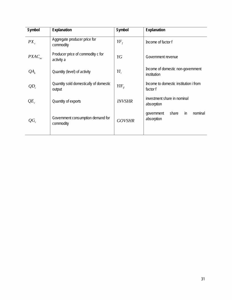
Symbol Explanation Symbol Explanation

Aggregate producer price for commodity

Income of factor f

Producer price of commodity c for activity a Government revenue

Quantity (level) of activity Income of domestic non-government institution

Quantity sold domestically of domestic output

Income to domestic institution i from factor f

cQE Quantity of exports INVSHR investment share in nominal absorption

Government consumption demand for commodity GOVSHR

government share in nominal absorption

cPX fYF

acPXAC YG

aQA iYI

cQD ifYIF

cQG

32

MODEL EQUATIONS Price and Production Equations

( ) ccCTc

cccc icmPQEXRtmpwmPM ''

'1 ×+×+×= ∑∈

(1)

( ) ccCTc

cccc icePQEXRtepwmPE ''

'1 ×−×−×= ∑∈

(2)

∑∈

×+=CTc

ccccc icdPQPDSPDD'

,''

(3)

( ) ccccccc QMPMQDPDDQQtqPQ ×+×=×−1

(4)

cccccc QEPEQDPDSQXPX ×+×=

(5)

caCc

caa PXACPA ,, θ×= ∑∈

(6)

acca icaPQPINTA ,∑=

(7)

( ) aaaaaaa QINTAPINTAQVAPVAQAtaPA ×+×=×−1

(8)

∑ ×= cwtsPQCPI c

(9)

dwtsPDSDPI c ×= ∑

(10)

( )( ) aa

aa

aa

aaaa

aa

aaa QINTAQVAQA ρρρ δδα

1

1−−− ×−+××=

(11)

aa

aa

aa

a

a

a

a

PVAPINTA

QINTAQVA ρ

δδ +

−

×=1

1

1

(12)

aaa QAivaQVA ×=

(13)

aaa QAaQINTA ×= int

(14)

vaava

a

Ffaf

vaaf

vaaa QFQVA

ρρδα

1

,,

−

∈

−

×= ∑

(15)

33

( ) 1,,

1

,,, 1 −−

−

∈

− ××

×××−=× ∑

vaa

vaa

afva

afFf

afva

afaaaaff QFQFQVAtvaPVAWFDISTWF ρρ δδ

(16)

aacac QINTAicaQINT ×= ,,

(17)

acaHh

hcaca QAQHAQXAC ×=+ ∑∈

,,,, θ

(18)

Commodities

11

,,

−−

−

∈

×= ∑

accac

cca

Aa

acca

accc QXACQX

ρρδα

(19)

1,,

1

,'

,,−−

−−

∈

×

××= ∑

acc

acc

caac

cacaAa

accaccca QXACQXACQXPXPXAC ρρ δδ

(20)

( )( ) tc

tc

tc

ctcc

tc

tcc QDQEQX ρυρ δδα

1

1 ×−+×=

(21)

11

1 −

×

−=

tc

c

ctc

tc

c

c

PDSPE

QDQE ρ

δδ

(22)

ccc QEQDQX +=

(23)

( )( ) qc

qc

qc

cqcc

qc

qcc QDQMQQ ρρρ δδα

1

1−−− ×−+×=

(24)

qc

qc

qc

c

c

c

c

PMPDD

QDQM ρ

δδ +

−

×=1

1

1

(25)

ccc QMQDQQ +=

(26)

( )∑∈

×+×+×=''

','','',Cc

cccccccccc QDicdQEiceQMicmQT

(27)

Institutions

afafAa

ff QFWFDISTWFYF ,, ××= ∑∈

(28)

34

( )[ ]EXRtrnsfrYFtfshifYIF frowfffifi ×−×−×= ,,, 1

(29)

EXRtrnsfrCPItrnsfrTRIIYIFYI rowigoviINSDNGi

iiFf

fii ×+×++= ∑∑∈∈

,,'

',,

(30)

( ) ( ) '''',', 11 iiiiiii YITINSMPSshiiTRII ×−×−×=

(31)

( ) ( ) hhhINSDNGi

hih YITINSMPSshiiEH ×−×−×

−= ∑

∈

111 ,

(32)

−−+=× ∑∑∑

∈ ∈∈ Aa Cc

hhcaca

Cc

mhcch

mhc

mhcchcc PXACPQEHPQQHPQ ,',',

',,,, γγβγ

(33)

−−+×=× ∑ ∑∑

∈ ∈ ∈Cc Aa Çc

hhcaca

mhcch

hhca

hhcacahcaca PXACPQEHPXACQHAPXAC

',,',,'',,,,,,,, .γγβγ

(34)

cc qinvIADJQINV ×=

(35)

cc qgGADJQG ×=

(36)

aaAa

aaaAa

afFf

fINSDNGi

ii QAPAtaQVAPVAtvaYFtfYITINSYG ××+÷×+×+×= ∑∑∑∑∈∈∈∈

cCc

cccCEc

ccccCMc

c QQPQtqEXRQEpweteEXRQMpwmtm ××+×××+×××+ ∑∑∑∈∈∈

EXRtrnsfrYIFFf

rowgovgov ×++ ∑∈

,

(37)

CPItrnsfrQGPQEGINSDNGi

govicCc

c ×+×= ∑∑∈∈

,

(38)

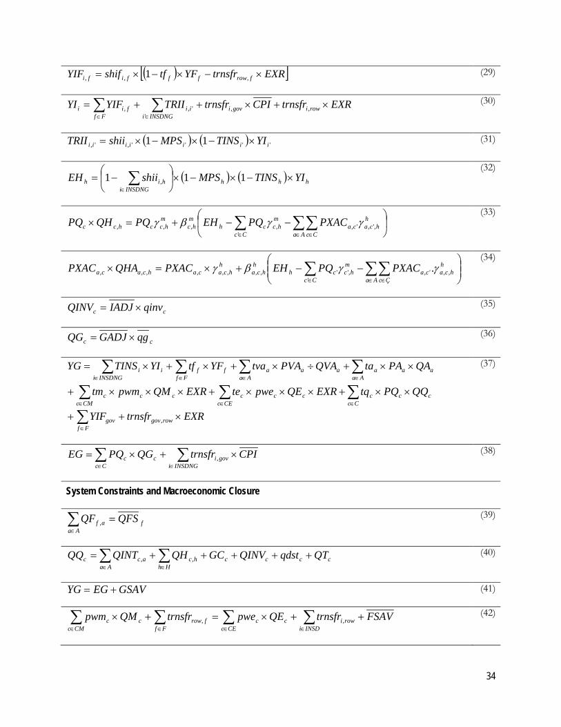
System Constraints and Macroeconomic Closure

fAa

af QFSQF =∑∈

,

(39)

ccccHh

hcAa

acc QTqdstQINVGCQHQINTQQ +++++= ∑∑∈∈

,,

(40)

GSAVEGYG +=

(41)

FSAVtrnsfrQEpwetrnsfrQMpwmINSDi

rowicCEc

cFf

frowcCMc

c ++×=+× ∑∑∑∑∈∈∈∈

,,

(42)

35

( ) =×++×−×∑∈

FSAVEXRGSAVYITINSMPS iiINSDNGi

i 1 cCc

ccCc

c qdstPQQINVPQ ×+× ∑∑∈∈

(43)

( ) tDTINStinsTINSADJtinsTINS ii ×+×+×= 011

(44)

( ) iiii mpsDPMSmpsMPSADJmpsMPS 01011 ×+×+×=

(45)

cCc

chcaAa Cc Hh

caHh Cc

hcc QGPQQHAPXACQHPQTABS ∑∑∑∑∑∑∈∈ ∈ ∈∈ ∈

+×+×= ,,,,

cCc

ccCc

c qdstPQQINVPQ ∑∑∈∈

+×+

(46)

cCc

ccCc

c qdstPQQINVPQTABSINVSHR ∑∑∈∈

+×=×

(47)

cCc

cQGPQTABGOVSHR ∑∈

=×

(48)