the importance of firms in wage determination max gruetter
TRANSCRIPT
IZA DP No. 1367
The Importance of Firms in Wage Determination
Max GruetterRafael Lalive
DI
SC
US
SI
ON
PA
PE
R S
ER
IE
S
Forschungsinstitutzur Zukunft der ArbeitInstitute for the Studyof Labor
October 2004
The Importance of Firms in Wage Determination
Max Gruetter University of Zurich
and IZA Bonn
Rafael Lalive University of Zurich,
CESifo and IZA Bonn
Discussion Paper No. 1367 October 2004
IZA
P.O. Box 7240 53072 Bonn
Germany
Phone: +49-228-3894-0 Fax: +49-228-3894-180
Email: [email protected]
Any opinions expressed here are those of the author(s) and not those of the institute. Research disseminated by IZA may include views on policy, but the institute itself takes no institutional policy positions. The Institute for the Study of Labor (IZA) in Bonn is a local and virtual international research center and a place of communication between science, politics and business. IZA is an independent nonprofit company supported by Deutsche Post World Net. The center is associated with the University of Bonn and offers a stimulating research environment through its research networks, research support, and visitors and doctoral programs. IZA engages in (i) original and internationally competitive research in all fields of labor economics, (ii) development of policy concepts, and (iii) dissemination of research results and concepts to the interested public. IZA Discussion Papers often represent preliminary work and are circulated to encourage discussion. Citation of such a paper should account for its provisional character. A revised version may be available directly from the author.
IZA Discussion Paper No. 1367 October 2004
ABSTRACT
The Importance of Firms in Wage Determination∗
Firms are central to many theories of the labor market. However, the extent to which firms affect wages has only recently been explored using matched employer-employee data. This paper investigates (i) the importance of firms in explaining wage differences across individuals and industries, and (ii) how the nature of interfirm mobility – job-to-job vs. job-unemployment-job – affects the relative importance of firms and workers in wage determination. Results indicate that (i) firms are much more important in explaining the variance of average wages across industries rather than individuals, and (ii) using job-to-job transitions reduces the importance of firm wage policies in explaining differences. JEL Classification: C23, J31 Keywords: interfirm mobility, wage determination, industry wage differentials, matched
employer employee data Corresponding author: Max Gruetter Institute for Empirical Research in Economics (IEW) University of Zurich Bluemlisalpstr. 10 8006 Zurich Switzerland Email: [email protected]
∗ We thank Erling Barth, Martin Brown, Harald Dale-Olsen, Alfred Garlo., Francis Kramarz, Edwin Leuven, David Margolis, Josef Zweimüller, and seminar participants at IEW, ISF, and IZA for comments on previous versions of this paper. Financial support by the Swiss National Science Foundation (No. 101412-103970) is gratefully acknowledged.

1 Introduction
”Is the variation between the price of labor in different plants almost as large as
the variation in hourly earnings, or is it considerably less?” (Slichter (1950), p. 90.)
Firms are central to many theories of the labor market. For instance, the classical view
emphasizing that wages reflect marginal productivity holds that wages differ across firms because
firms utilize capital to different degrees or offer workplaces that differ with respect to amenities
(Rosen (1986); Cahuc, Gianella, Goux, and Zylberberg (2002)). Since wages may be the carrot
that motivates employees to provide effort firms that find it hard to monitor workers offer
higher wages – the efficiency wage view (Shapiro and Stiglitz (1984), Krueger and Summers
(1987)). The theory of the labor market emphasizing institutions argues that differences in
unionization rates explain wage differences across firms (Booth (1995), Margolis and Salvanes
(2001)). Equilibrium search theory rationalizes wage differentials across firms for homogenous
workers due to search frictions (Burdett and Mortensen (1998); van den Berg and Ridder (1998);
Postel-Vinay and Robin (2002); Mortensen (2003)). Finally, since the elasticity of labor supply
facing the firm is finite, monopsony theory also rationalizes a strong role for firms in wage
determination (Manning (2003)). Indeed, Slichter (1950) argues that the answer to his question
cited above allows ”to speculate concerning the effects of the wage structure upon the distribution
of resources among places, firms, and industries.” (p. 90)
However, for a long time period, it was not possible to assess the actual wage setting policy
of firms because the available micro data-sets did not allow separating the ’price of labor across
plants’ from the effect of skill differences across workers. The seminal work by Abowd, Kramarz,
and Margolis (1999b) used matched employer-employee compensation information to provide a
first assessment of the relative importance of firms and workers in wage determination for France.
Using an approximate method they show that personal heterogeneity is far more important in
explaining variations in the wage rates across individuals as well as across industries.1 Abowd,
Creecy, and Kramarz (2002) state in a subsequent study using the exact solution instead of the
approximate solution that the results for individuals but not for industries are robust. Thus
the approximate method is sensitive to an underspecified conditioning matrix. All existing
studies suffer from the problem that the mobility decision which is essential to disentangle the
person and the firm component is modelled exogenous but the data used are not controlled for
endogenous mobility.
This paper reassesses the method developed by Abowd, Kramarz, and Margolis (1999b) using
a modified version of the exact method in Abowd, Creecy, and Kramarz (2002) and discussing
1Further studies have investigated differences between the U.S. and France (Abowd and Kramarz (1999)).The results differ slightly in the sense that firm’s and worker’s heterogeneity are comparably important on theindustry level in the U.S..
2
the relevance of endogenous mobility. First, we introduce a new statistic to document the
extent to which firms contribute to wage differences. We define the importance of firms in wage
determination as the share of the total variance that is due to the firm’s wage policy – a concept
that is directly inspired by Slichter’s 1950 question.2 We then use this novel statistic to contrast
the extent to which differences in wage policies across individual firms explain the total variance
in wage rates with the importance of firms in explaining industry wage differences. This contrast
allows inferring more closely to what extent the industry category reflects firm differences rather
than worker differences. In contrast to Abowd, Kramarz, and Margolis (1999b) our findings
indicate that firms are much more important in explaining the variance in average wages across
industries than across individuals. Whereas firms account for about one quarter of the total
variance in individual wage rates, industry average firm wage policies contribute three quarters
of the total variance of average wages across industries. Thus industries are a relatively good
proxy for firms.
In a second step, we discuss how the nature of interfirm mobility affects the relative impor-
tance of firms and workers in wage setting. Intuitively, the wage policy of the firm is revealed
when workers move between firms. This paper argues that it is useful to distinguish between
at least two fundamentally distinct types of interfirm mobility3 in order to study the degree
to which endogenous mobility affects identification of the firm’s wage policy: job-to-job (JTJ)
transitions on the one hand and job-unemployment-job (JUJ) transitions on the other hand.
Workers changing directly from one employer to another employer are likely to do so because
the new employer offers a superior wage rate. Thus, the wage change due to a JTJ transition
reflects both, the wage policy of the new firm as well as the wage policy of the previous employer.
In contrast, workers who enter unemployment between jobs compare the wage rate offered with
income while unemployed. To the extent that unemployment benefits are actually lower than
income on the previous job, the wage rate in the previous job is less important for the wage
rate accepted by the unemployed worker than for the wage rate accepted by a job-to-job mover.
Findings indicate that reliance on JTJ mobility in identifying firms’ wage policies leads to a
reduction in firms’ importance in wage determination.
This paper is closely related to two important strands of the literature. First, the literature
on wage determination has focused strongly on industry wage differentials. Originally, Slichter
(1950) investigated industry wage differentials for relatively homogenous male unskilled labor
in order to detect the basic forces that shape the wage structure. The idea was that, if these
workers are indeed completely homogenous, these industry wage differentials reflect differences
in the ”typical” wage policy of firms across industries. Subsequently, a large body of the lit-
erature has built up that investigated the original results of strong variation in average wages
2In contrast, the existing literature uses the correlation between wages and the firms’ wage policies to discussthe relevance of firms in wage setting. The correlation statistic can not be interpreted as the share of the totalvariance in wage rates that is due to firms. Groshen (1991) also uses this concept.
3Note that we use the term inter-firm mobility and job mobility synonymously in the remainder of this paper.
3
across industries for different countries, time periods, and with more rigorous statistical meth-
ods (Murphy and Topel (1987), Krueger and Summers (1987), Krueger and Summers (1988),
Dickens and Katz (1987)).4 Arguing that industry mobility is endogenous, important work by
Gibbons and Katz (1992) discusses whether or not industry wage differentials reflect remuner-
ation for skills or pure rents.5 This paper contributes to the inter-industry wage differentials
literature in contrasting the extent to inter-industry wage differences reflect firm wage setting
with the individual level. Second, our paper is closely related to the literature that studies
the inter-relationship between wage growth and labor mobility (Antel (1991), Topel and Ward
(1994), Farber (1999)). We study the extent to which differences in inter-firm mobility lead to
different conclusions regarding the importance of firms in wage setting. This contrast is inspired
by the literature that discusses endogenous job mobility and industry wage setting (Gibbons
and Katz (1992)). The novel feature of our analysis is, however, that we rely on the two most
common types of inter-firm mobility – job-to-job and job-unemployment-job mobility – rather
than the much more seldom mobility due to plant closure. This is advantageous for the purpose
of this paper since we aim at decomposing wages into worker and firm effects for as large a share
of the underlying population of firms and workers as possible.6
The empirical analysis is based on a matched employer-employee dataset that covers a 25 %
random sample of men working 1990 until 19977 in Austria. This main dataset contains infor-
mation on total compensation, various demographic characteristics, and a workplace identifier.
A total of 2,090,483 observations cover 378,244 different persons and 103,346 firms. The analysis
is also based on two sub-samples of movers in order to discuss the extent to which inter-firm mo-
bility affects identification of firms’ contribution to wage setting. The job-to-job (JTJ) sample
considers workers who have moved between employers at least once and always did so directly
from job to job. The job-unemployment-job (JUJ) sample considers all workers who have moved
between employers at least once and all moves between jobs involved a spell of unemployment.
The crucial difference between both sample is that all persons in the JTJ sample changed their
job voluntary while all persons in the JUJ sample had to change employers because they had to
find a new job. Because the conditioning method proposed in Abowd, Kramarz, and Margolis
(1999b) is not robust, all results are based on a modified version of the exact method in Abowd,
Creecy, and Kramarz (2002) that decomposes the wage rate into a worker component, a firm
4See for example Carruth, Collier, and Dickerson (1999) for the UK, Goux and Maurin (1999) for France,Vainiomki and Laaksonen (1995) for Finland or Winter-Ebmer (1994) for Austria. Kahn (1998) and Zweimuellerand Barth (1994) study the inter-relationship between industry wage differences and unionization rates.
5Recently, Gibbons, Katz, Lemieux, and Parent (2002) extend the original Gibbons and Katz (1992) framework.Kim (1998) argues that industry wage differentials reflect compensation for match specific productivity.
6The potential cost to taking this perspective is identification. However, note that under some conditions thatwe discuss in the following section, contrasting the most common types of inter-firm mobility suffices to identifythe extent to which endogenous mobility affects the importance of firms in wage setting.
7We use Oktober 10 as valuation date because this is a date where neither the summer nor the winter tourismis dominant.
4
component, and a transitory component.
The following section presents the statistical model, provides the definition of the importance
of firms in wage determination, and discusses endogenous mobility. In section 3, we describe
the data, discuss the main variables, and present descriptive analysis of wage differentials and
the patterns of job mobility across 39 industries in Austria. Section 4 presents the main results,
and section 5 concludes.
2 Measuring Firm Wage Policies
This section discusses the decomposition of the log of the wage rate into a worker effect, a firm
effect, and an error term. Having these effects in hand we define how we measure the importance
of firms in wage setting. In a last step we show via an example the consequence of interfirm
mobility on the estimation of the coefficients.
2.1 Decomposing Wages
Let yit be the log of the wage rate of worker i at time t, let xit denote the time-varying charac-
teristics, let sJ(it)denote years of seniority of worker i at time t, and let J(i, t) be the employer
identification number of worker i at time t. The number of workers in the dataset is N, the
number of firms is J , and the number of observations is N∗. We assume that
yit = xitβ + θi + φJ(i,t) + γJ(i,t)sJ(it) + εit (1)
and
E[εit|i, t, J(i, t), xit] = 0 (2)
The wage policy of the firm is modelled as simple as possible.8 The entry wage, φj , captures
the wage differential earned in the present firm compared to the average firm in the dataset
(j = 1, ..., J). The tenure effect, γj , captures differences across firms in the wage increases
due to changes in seniority (j = 1, ..., J). Thus, the contribution of the firm to the wage rate
of worker i in period t is ψit ≡ φJ(i,t) + γJ(i,t)sit. The worker’s wage component, θi, reflects
differences in pay due to time-invariant characteristics of each worker (i = 1, ..., N). Thus, θi
measures the extent to which compensation for skill is important. Finally, the parameter β
measures economy-wide returns to experience or productivity increases (see following section
for a definition of X).
The main statistical assumption is exogenous mobility in equation (2). This assumption
rules out any correlation between unmeasured time-varying effects on the wage rate captured
by εit with the person effect θi, the firm effects or the time-varying observed effects xit .
8A more elaborate model for the wage policy allows for non-linearity in returns to seniority. However, keepingthe wage policy of the firm as simple as possible allows identifying the wage policy for a large number of firms.
5

Direct estimation of the model (1) by least squares is difficult due to computer memory
constraints (Abowd, Kramarz, and Margolis (1999b)). This paper uses a modified version of
the iterative algorithm proposed in Abowd, Creecy, and Kramarz (2002) to solve for the least
squares parameter estimates β̂, θ̂i, φ̂j , and γ̂j (see appendix for a description of our algorithm).
2.2 The Importance of Firms in Wage Determination
We propose to measure the importance of firms in wage setting by the contribution of firms
to the overall variance in wage rates. In introducing this statistic, note that the total variance
in wages var(yit) can be decomposed into a term reflecting covariance of the wage rate with
the wage policy of the firm, covariance of the wage rate with worker skills, and covariance
of the wage rate with the transitory component of wage rates, i.e. var(yit) = cov(yit, yit) =
cov(yit, ψ̂it) + cov(yit, θ̂i + xitβ̂) + cov(yit, ε̂it). Thus, defining the importance of firms in wage
setting as the covariance between the firms’ contribution with the wage rate relative to the
overall variance
ν̂f ≡ cov(yit, ψ̂it)var(yit)
=var(ψ̂it)var(yit)
+cov(xitβ̂ + θ̂i, ψ̂it)
var(yit)(3)
ensures a full decomposition of the total variance in wage rates into a firm component, ν̂f ,
a worker component, ν̂p ≡ cov(yit, xitβ̂ + θ̂i)/var(yit), and a transitory component, ν̂ε.9 A
useful interpretation of ν̂f is the following. The importance of firms predicts the (unobserved)
expected difference in the firms’ contribution ψ̂it as a function of the (observed) wage rate. This
is true because ν̂f gives the derivative of the conditional expectation of the firm’s contribution to
wages due to a change in the wage rate in a linear regression framework, i.e. ∂E(ψ̂it|yit)/∂yit =
cov(yit, ψ̂it)/var(yit).10
Equation (3) shows that firms can be important in wage determination for two reasons. First,
firms generate strong wage differentials if there are weightily reasons for firms to offer different
wages to observationally equivalent workers. This reason shows up as a high relative variance of
the firms’ contribution. This variance term (var(ψ̂it)/var(yit)) also answers directly Slichter’s
(1950) question cited in the introduction. Second, firms can also amplify the total variance in
wage rates in attracting more productive workers. This second reason shows up as a strong
covariance term. Note that from the labor economists point of view, assessing the relative
importance of these two reasons is important. Whereas strong variance in the firm specific
wage component lends support to theories emphasizing the reasons for different compensation
packages, strong covariance is in support of other theories that explain how workers and firms
9Note that the covariance between the firm’s contribution �ψit with the error term �εit is zero by virtue ofexogenous mobility imposed on the estimates by least squares.
10For instance, suppose two workers are employed in different firms with worker 1 earning w1 and worker 2earning w2. We can say that the firms’ contribution is expected to differ by �νf (w1 − w2).
6
are matched on the labor market.11
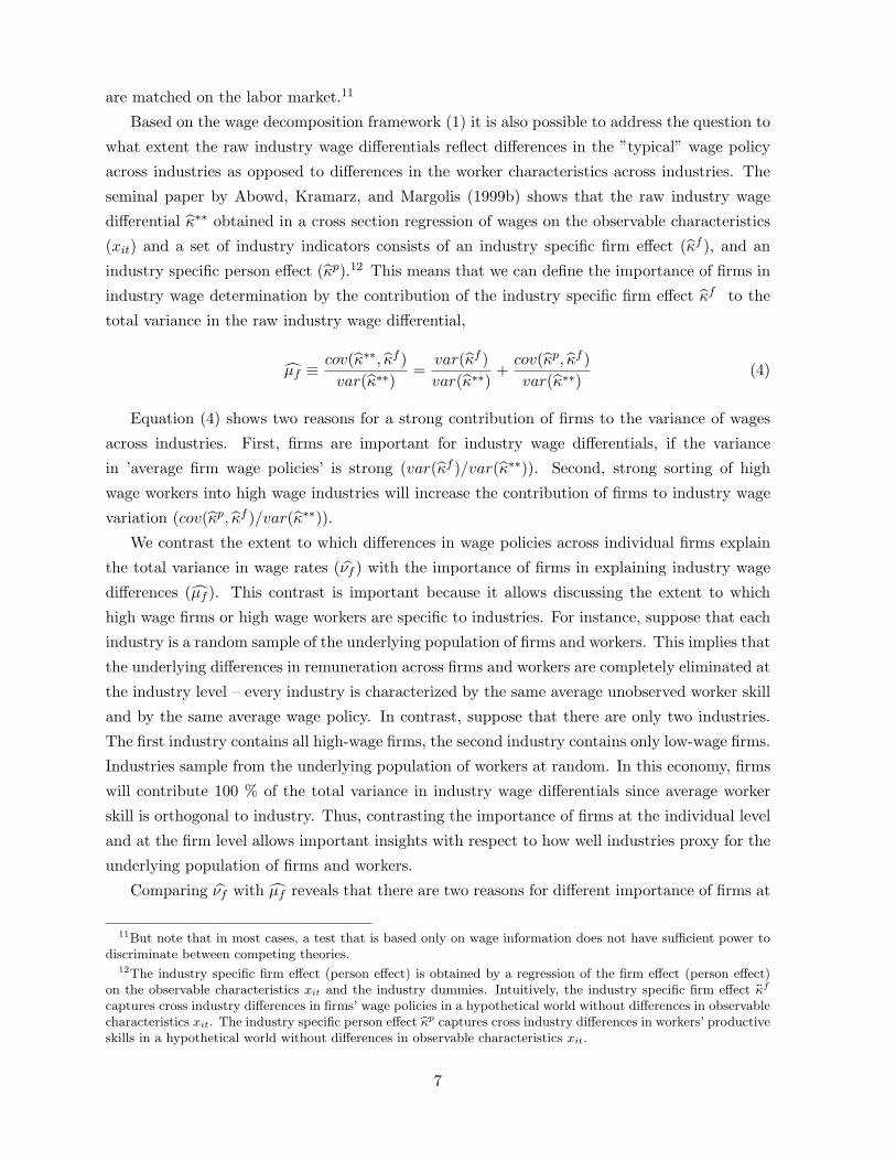
Based on the wage decomposition framework (1) it is also possible to address the question to
what extent the raw industry wage differentials reflect differences in the ”typical” wage policy
across industries as opposed to differences in the worker characteristics across industries. The
seminal paper by Abowd, Kramarz, and Margolis (1999b) shows that the raw industry wage
differential κ̂∗∗ obtained in a cross section regression of wages on the observable characteristics
(xit) and a set of industry indicators consists of an industry specific firm effect (κ̂f ), and an
industry specific person effect (κ̂p).12 This means that we can define the importance of firms in
industry wage determination by the contribution of the industry specific firm effect κ̂f to the
total variance in the raw industry wage differential,
µ̂f ≡ cov(κ̂∗∗, κ̂f )var(κ̂∗∗)
=var(κ̂f )var(κ̂∗∗)
+cov(κ̂p, κ̂f )var(κ̂∗∗)
(4)
Equation (4) shows two reasons for a strong contribution of firms to the variance of wages
across industries. First, firms are important for industry wage differentials, if the variance
in ’average firm wage policies’ is strong (var(κ̂f )/var(κ̂∗∗)). Second, strong sorting of high
wage workers into high wage industries will increase the contribution of firms to industry wage
variation (cov(κ̂p, κ̂f )/var(κ̂∗∗)).We contrast the extent to which differences in wage policies across individual firms explain
the total variance in wage rates (ν̂f ) with the importance of firms in explaining industry wage
differences (µ̂f ). This contrast is important because it allows discussing the extent to which
high wage firms or high wage workers are specific to industries. For instance, suppose that each
industry is a random sample of the underlying population of firms and workers. This implies that
the underlying differences in remuneration across firms and workers are completely eliminated at
the industry level – every industry is characterized by the same average unobserved worker skill
and by the same average wage policy. In contrast, suppose that there are only two industries.
The first industry contains all high-wage firms, the second industry contains only low-wage firms.
Industries sample from the underlying population of workers at random. In this economy, firms
will contribute 100 % of the total variance in industry wage differentials since average worker
skill is orthogonal to industry. Thus, contrasting the importance of firms at the individual level
and at the firm level allows important insights with respect to how well industries proxy for the
underlying population of firms and workers.
Comparing ν̂f with µ̂f reveals that there are two reasons for different importance of firms at
11But note that in most cases, a test that is based only on wage information does not have sufficient power todiscriminate between competing theories.
12The industry specific firm effect (person effect) is obtained by a regression of the firm effect (person effect)on the observable characteristics xit and the industry dummies. Intuitively, the industry specific firm effect �κf
captures cross industry differences in firms’ wage policies in a hypothetical world without differences in observablecharacteristics xit. The industry specific person effect �κp captures cross industry differences in workers’ productiveskills in a hypothetical world without differences in observable characteristics xit.
7

the individual and at the industry level. First, the relative variance of the firm’s contribution
at the individual level and at the aggregate level can differ. Second, differential sorting of
individuals across firms can explain why firms contribute more strongly at the aggregate level
compared to the individual level even if relative variances are constant.
2.3 Endogenous Mobility: Example
We discuss how the nature of interfirm mobility affects estimates of φ, and γ and thus the
relative importance of firms and workers in wage setting. In order to discuss why job mobility
might affect the estimated worker and firm effects consider the following example. Suppose, for
simplicity, homogenous individuals with respect to xit and θi (these parameters are normalized to
0), and firms which differ only with respect to a time-invariant wage component φj . Additionally
suppose that there are just two points of time 0 and 113 and that at time 0 there is just one
firm with index 1. The wage rate at time 0 is yi0 = φ1 + εi0, where εi0 reflects the random
component of productivity of worker i at time 0. At time 1, all workers get an outside wage
offer y∗i1 = φj + ε∗i1, j = 2...J . Workers are assumed to earn the wage they earned at time 0
if they decide to stay with their employer at time 1.14 All random shocks to productivity are
i.i.d. If we abstract from additional amenities or disamenities of jobs, workers will move from
employer 1 to employer j if the outside wage offer exceeds the inside wage offer
φj + ε∗i1 ≥ φ1 + εi0 (5)
Observed wage rates at time 1 are then given by yi1 = I(φj+ε∗i1 ≥ φ1+εi0)y∗i1+(1−I(φj+ε∗i1 ≥φ1 + εi0))yi0 where I(A) is the indicator function taking the value 1 if A is true and 0 otherwise.
The least squares estimator identifies the effect of firm j on wages relative to firm 1 based on
the expected wage change for movers from firm 1 to firm j15
E(yi1 − yi0|J(i, 1) = j, J(i, 0) = 1) = φj − φ1 +
+ E(ε∗i1 − εi0|ε∗i1 − εi0 ≥ −(φj − φ1)) (6)
This shows first, that the estimator of the firm effect is biased upward since E(ε∗i1−εi0|ε∗i1−εi0 ≥−(φj −φ1)) > 0. Second, the smaller the true relative firm effect (φj −φ1) is, the stronger is the
upward bias in the estimated firm effect. As a result, the variance in the firm effect identified
with JTJ transitions tends to be smaller than the variance in the true firm effects thereby
13As in our dataset we use the concept of points in time where we observe the individuals. Thus between time0 and 1 there are several days where we do not observe the individuals but at time 1 we have information on whathappened between time 0 and 1.
14This assumption is made for simplicity. All results hold at the qualitative level if the wage rate at time 1 isa new random draw from the firm specific wage distribution.
15See Abowd, Creecy, and Kramarz (2002) for a more exhaustive treatment of identification of worker and firmeffects.
8
reducing the explanatory power of firms in wage determination.
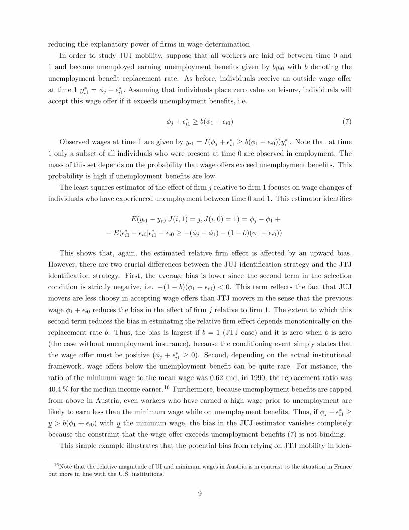
In order to study JUJ mobility, suppose that all workers are laid off between time 0 and
1 and become unemployed earning unemployment benefits given by byi0 with b denoting the
unemployment benefit replacement rate. As before, individuals receive an outside wage offer
at time 1 y∗i1 = φj + ε∗i1. Assuming that individuals place zero value on leisure, individuals will
accept this wage offer if it exceeds unemployment benefits, i.e.
φj + ε∗i1 ≥ b(φ1 + εi0) (7)
Observed wages at time 1 are given by yi1 = I(φj + ε∗i1 ≥ b(φ1 + εi0))y∗i1. Note that at time
1 only a subset of all individuals who were present at time 0 are observed in employment. The
mass of this set depends on the probability that wage offers exceed unemployment benefits. This
probability is high if unemployment benefits are low.
The least squares estimator of the effect of firm j relative to firm 1 focuses on wage changes of
individuals who have experienced unemployment between time 0 and 1. This estimator identifies
E(yi1 − yi0|J(i, 1) = j, J(i, 0) = 1) = φj − φ1 +
+ E(ε∗i1 − εi0|ε∗i1 − εi0 ≥ −(φj − φ1) − (1 − b)(φ1 + εi0))
This shows that, again, the estimated relative firm effect is affected by an upward bias.
However, there are two crucial differences between the JUJ identification strategy and the JTJ
identification strategy. First, the average bias is lower since the second term in the selection
condition is strictly negative, i.e. −(1 − b)(φ1 + εi0) < 0. This term reflects the fact that JUJ
movers are less choosy in accepting wage offers than JTJ movers in the sense that the previous
wage φ1 + εi0 reduces the bias in the effect of firm j relative to firm 1. The extent to which this
second term reduces the bias in estimating the relative firm effect depends monotonically on the
replacement rate b. Thus, the bias is largest if b = 1 (JTJ case) and it is zero when b is zero
(the case without unemployment insurance), because the conditioning event simply states that
the wage offer must be positive (φj + ε∗i1 ≥ 0). Second, depending on the actual institutional
framework, wage offers below the unemployment benefit can be quite rare. For instance, the
ratio of the minimum wage to the mean wage was 0.62 and, in 1990, the replacement ratio was
40.4 % for the median income earner.16 Furthermore, because unemployment benefits are capped
from above in Austria, even workers who have earned a high wage prior to unemployment are
likely to earn less than the minimum wage while on unemployment benefits. Thus, if φj + ε∗i1 ≥y > b(φ1 + εi0) with y the minimum wage, the bias in the JUJ estimator vanishes completely
because the constraint that the wage offer exceeds unemployment benefits (7) is not binding.
This simple example illustrates that the potential bias from relying on JTJ mobility in iden-
16Note that the relative magnitude of UI and minimum wages in Austria is in contrast to the situation in Francebut more in line with the U.S. institutions.
9
tifying the contribution of firms to wage rates is potentially important and that this bias is
correlated negatively with the magnitude of the relative firm effect. In contrast, identification
based on JUJ mobility tends to be affected less strongly by endogenous mobility bias. It is
important to keep in mind that this simple example is meant to illustrate the potential implica-
tions of JTJ relative to JUJ mobility. It is obvious that the example abstracts from a number
of important features encountered on actual labor markets such as differences across workers in
observed time-varying characteristics, unobserved time-constant characteristics, the existence of
multiple firms at time 0, and simultaneous occurrence of JTJ and JUJ mobility. Nevertheless,
it is unlikely that the insight regarding the relative bias due to JTJ and JUJ mobility is altered
at the qualitative level.
We discuss the extent to which inter-firm mobility affects the importance of firms in wage
determination by contrasting two samples of movers. The first sample considers workers who
have moved between employers at least once and always did so directly from job-to-job – the JTJ
sample. The second sample is identical to the first sub-sample with the exception that workers
have experienced a spell of unemployment between jobs – the JUJ sample. We then apply the
wage decomposition algorithm, separately, to the JTJ sample and to the JUJ sample. This gives
two sets of parameter estimates, the first being identified solely based on job-to-job mobility,
the second being based, exclusively, on job-unemployment-job mobility. This means that we
can assess the relevance of inter-firm mobility for the wage decomposition (1) by contrasting the
importance of firms in the JTJ sample to the importance of firms in the JUJ sample (both at the
individual and at the industry level). The difference in the two statistics provides information
on the extent to which the importance of firms in wage setting is sensitive due to the fact that
identification relies fully on JTJ mobility (JTJ sample) as opposed to identification ruling out
JTJ mobility completely (JUJ sample). Thus, this comparison is informative on the maximum
extent to which endogenous mobility affects the importance of firms in wage determination.
3 Data
We use Austrian social security data (ASSD) to study the relevance of firms in wage setting
and discuss the role of inter-firm mobility. This data set is ideally suited to study the issue
of job mobility in determining firm wage components as it allows us to trace the individuals’
complete earnings and employment history. Not only sequences of jobs but also intermediate
spells of unemployment can be observed. Our sample covers 25% of all individuals who were
ever employed in the private sector in Austria on October 10th in the period between 1990 and
1997. This data contains information on employment (blue/white collar, tenure, experience),
earnings, and the identification number of the employer. In addition, there is information on
gender and date of birth for each individual. Incomplete data on nationality and education
can be inferred from the Austrian unemployment register for those individuals who ever enter
10
unemployment in the period from 1986 until 1997.
The analysis is restricted to male employees between 25 years and 55 years for two reasons.
First, the data set does not provide information on working hours. At 25 years of age, most
individuals have completed their education and are able to work full-time.17 Second, early
retirement starts at age 60 (for males) and 55 (for females). In order to rule out early retirement
effects we focus on an age group that is below the early retirement age.18 We focus only on
those employees who were working and focus on the job with the highest earnings in the case
of multiple jobs.19 Using these selection criteria our data-set includes 2,090,483 observation of
378,244 different persons and 103,346 firms.
We discuss the effect of identifying the wage decomposition based on JTJ mobility as opposed
to JUJ mobility. The impact of JTJ mobility relative to JUJ mobility can be studied in the
following two sub-samples
• The JUJ sample contains all individuals who changed jobs at least once and always ex-
perienced a spell of unemployment between successive jobs. A job change occurs if the
employer in one year is different from the employer in the preceding year.20 The idea is
that, in the JUJ sample, the wage rate in the previous job is likely to play a minor role in
determining the wage rate in the new job. The JUJ sample contains 299,310 observations
of 54,991 different individuals and 51,630 different firms.
• The JTJ sample contains all individuals who changed their job at least once but never
through unemployment. The idea is that, in the JTJ sample, job mobility is driven by
the new wage rate exceeding the wage rate in the previous job. For instance workers who
happen to be matched with a high wage employer will only be induced to change to a
new employer if that employer offers an even higher wage rate. Thus this sample likely
to contain endogenous mobility. The JTJ sample contains 441,900 observations of 68,678
different individuals and 54,586 firms.
• By construction, no individual shows up in both, the JTJ and the JUJ sample. However,
21,352 firms are common to both sub-samples. We will use this overlap in the data to
answer our second question, the effect of interfirm mobility.
Austrian labor law forces employers to notify workers of a pending layoff three months in
advance. Since we can not infer from the data whether or not the worker is laid off or quits, we
17According to Statistics Austria, only 2.36 % of all male employees aged 25 to 54 are part-time workers, but25.0 % of all employed women work part-time.
18Note that basically due to disability insurance already about 20% of all men have terminated their workingcareer at the age of 55.
19Multiple job holders make up less than 1 % of the dataset.20This classification means that if an employee changed within a year away from his old employer and than
back again, this would not count as a job change. Also so called recalls (from unemployment) do not count asjob changes.
11
possibly allocate some workers into the JTJ sample who were actually faced with a permanent
layoff. However, note that such mis-allocation will tend to bias our contrast of the JUJ sample
with the JTJ sample towards finding a zero effect. Thus, our results can be understood as
giving a lower bound on the actual relevance of inter-firm mobility. Moreover, contrasting the
JTJ with the JUJ sample can, potentially, be difficult since this contrast not only reflects inter-
firm mobility but also different composition of the JUJ and the JTJ sample. We address the
relevance of this concern in section 4.
3.1 Construction of Main Variables
This sub-section describes the main variables used in the following empirical analysis. We
concentrate on those variables which needed to be constructed.
The dataset contains information on annual earnings. Because we also know the number
of days worked within a year, the dependent variable is the log of deflated income per day
worked, the ’daily wage’.21 Because there is an upper contribution limit to the state pension
system in Austria, annual earnings are top coded. Top coding affects roughly 15 % of all income
information. In order to address the top-coding problem, we construct a cluster of 1,440 cells
based on age, experience, place of work, blue collar or white collar and year. Then, we estimate
a tobit regression for each cell with log wage as the dependent variable and a constant as the
only regressor. This yields the moments of the distribution of a censored normal variable that
fits the wage distribution best within each cell. With this information we can impute, for all
individuals with a wage above the limit, the daily wage by the expectation of the upper tail of
the truncated distribution.
We define previous work experience and job tenure as the number of days actually worked
since 1972 instead of using potential labor force experience. To allow for a flexible experience
profile we recode work experience into eight different categories (0, 1, 2-3, 4-5, 6-8, 9-12, 13-17,
18+ years of experience). Because of the known insurance type we can distinguish between blue
and white collar workers.22
12
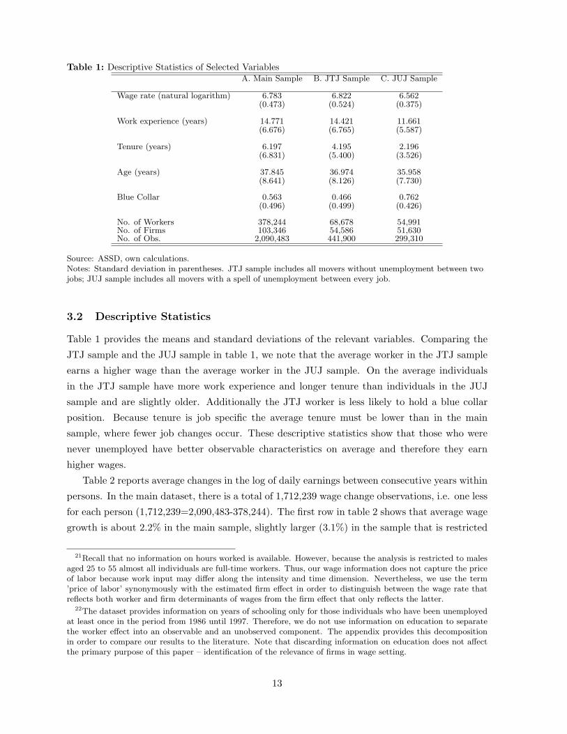
Table 1: Descriptive Statistics of Selected VariablesA. Main Sample B. JTJ Sample C. JUJ Sample
Wage rate (natural logarithm) 6.783 6.822 6.562(0.473) (0.524) (0.375)
Work experience (years) 14.771 14.421 11.661(6.676) (6.765) (5.587)
Tenure (years) 6.197 4.195 2.196(6.831) (5.400) (3.526)
Age (years) 37.845 36.974 35.958(8.641) (8.126) (7.730)
Blue Collar 0.563 0.466 0.762(0.496) (0.499) (0.426)
No. of Workers 378,244 68,678 54,991No. of Firms 103,346 54,586 51,630No. of Obs. 2,090,483 441,900 299,310
Source: ASSD, own calculations.Notes: Standard deviation in parentheses. JTJ sample includes all movers without unemployment between twojobs; JUJ sample includes all movers with a spell of unemployment between every job.
3.2 Descriptive Statistics
Table 1 provides the means and standard deviations of the relevant variables. Comparing the
JTJ sample and the JUJ sample in table 1, we note that the average worker in the JTJ sample
earns a higher wage than the average worker in the JUJ sample. On the average individuals
in the JTJ sample have more work experience and longer tenure than individuals in the JUJ
sample and are slightly older. Additionally the JTJ worker is less likely to hold a blue collar
position. Because tenure is job specific the average tenure must be lower than in the main
sample, where fewer job changes occur. These descriptive statistics show that those who were
never unemployed have better observable characteristics on average and therefore they earn
higher wages.
Table 2 reports average changes in the log of daily earnings between consecutive years within
persons. In the main dataset, there is a total of 1,712,239 wage change observations, i.e. one less
for each person (1,712,239=2,090,483-378,244). The first row in table 2 shows that average wage
growth is about 2.2% in the main sample, slightly larger (3.1%) in the sample that is restricted
21Recall that no information on hours worked is available. However, because the analysis is restricted to malesaged 25 to 55 almost all individuals are full-time workers. Thus, our wage information does not capture the priceof labor because work input may differ along the intensity and time dimension. Nevertheless, we use the term’price of labor’ synonymously with the estimated firm effect in order to distinguish between the wage rate thatreflects both worker and firm determinants of wages from the firm effect that only reflects the latter.
22The dataset provides information on years of schooling only for those individuals who have been unemployedat least once in the period from 1986 until 1997. Therefore, we do not use information on education to separatethe worker effect into an observable and an unobserved component. The appendix provides this decompositionin order to compare our results to the literature. Note that discarding information on education does not affectthe primary purpose of this paper – identification of the relevance of firms in wage setting.
13

Table 2: Descriptive Statistics: Log Wage ChangesA. Main Sample B. JTJ Sample C. JUJ Sample
Total 0.022 0.031 0.008(0.184) (0.239) (0.232)
Stayer 0.024 0.026 0.023(0.119) (0.135) (0.116)
JTJ Transitions 0.050 0.044 -(0.403) (0.422) -
JUJ Transitions -0.031 - -0.023(0.374) - (0.367)
Share of JTJ Transitions 51.62 100.00 0.00No. of Obs. 1,712,239 373,222 244,319
Source: ASSD, own calculations.Notes: Standard deviation in parentheses. JUJ is a job-unemployment-new job transition, JTJ is a job new jobtransition. See notes table 1 for a definition of the sub-samples.
to individuals who are observed to move between firms without entering unemployment (JTJ
sample), and wage growth is almost zero (0.8 %) in the dataset containing individuals who
always change via unemployment (JUJ sample). Interestingly, the second row in table 2 shows
that these differences in average wage growth are not due to differences in wage growth for
stayers. Thus, both sub-datasets are comparable to the main dataset in terms of stayer wage
growth. The third and the fourth row report average wage changes for JTJ transitions and JUJ
transitions, respectively. A striking picture emerges. Whereas wage growth is about twice as
high for individuals moving directly between firms compared to stayers (5.0% vs 2.4%), average
wage growth is significantly negative for JUJ transitions (-3.1%) in the main dataset. Results for
the sub-datasets show that the average JTJ transition in the JTJ dataset commands a similar
wage increase as the average JTJ transition in the main dataset (4.4% vs 5.0%). A similar
conclusion holds for the average JUJ transition (-2.3% vs -3.1%). These results suggest that
contrasting the wage decomposition obtained in the JTJ sample with the decomposition obtained
in the JUJ sample is informative on the extent to which a wage decomposition is affected by
JTJ mobility.23 The idea is that the wage decomposition in the JTJ dataset relies exclusively on
JTJ transitions in identifying the firms’ wage policy. In contrast, in the JUJ dataset, the firms’
wage policy is identified by transitions which are more in line with the underlying experiment
that defines the wage policy, i.e. with the experiment of placing workers into firms at random.
3.3 Industry Wage Differentials in Austria
Regressing the log wage rate on industry affiliation of the employer and experience, age, tenure
(and the squared of these), education, year dummies and blue collar status yields the industry
23Note that this contrast needs to account for the fact that workers as well as firms differ across the sub-samples.We discuss a way to account for selectivity in the following section.
14
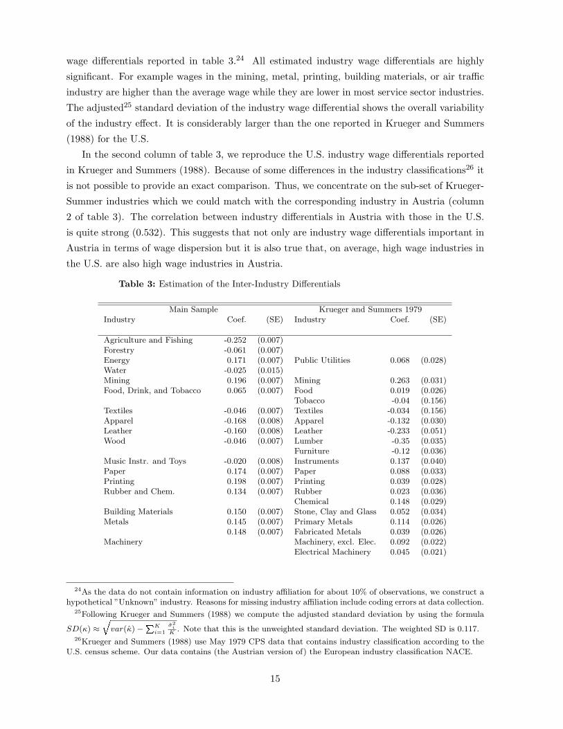
wage differentials reported in table 3.24 All estimated industry wage differentials are highly
significant. For example wages in the mining, metal, printing, building materials, or air traffic
industry are higher than the average wage while they are lower in most service sector industries.
The adjusted25 standard deviation of the industry wage differential shows the overall variability
of the industry effect. It is considerably larger than the one reported in Krueger and Summers
(1988) for the U.S.
In the second column of table 3, we reproduce the U.S. industry wage differentials reported
in Krueger and Summers (1988). Because of some differences in the industry classifications26 it
is not possible to provide an exact comparison. Thus, we concentrate on the sub-set of Krueger-
Summer industries which we could match with the corresponding industry in Austria (column
2 of table 3). The correlation between industry differentials in Austria with those in the U.S.
is quite strong (0.532). This suggests that not only are industry wage differentials important in
Austria in terms of wage dispersion but it is also true that, on average, high wage industries in
the U.S. are also high wage industries in Austria.
Table 3: Estimation of the Inter-Industry Differentials
Main Sample Krueger and Summers 1979Industry Coef. (SE) Industry Coef. (SE)
Agriculture and Fishing -0.252 (0.007)Forestry -0.061 (0.007)Energy 0.171 (0.007) Public Utilities 0.068 (0.028)Water -0.025 (0.015)Mining 0.196 (0.007) Mining 0.263 (0.031)Food, Drink, and Tobacco 0.065 (0.007) Food 0.019 (0.026)
Tobacco -0.04 (0.156)Textiles -0.046 (0.007) Textiles -0.034 (0.156)Apparel -0.168 (0.008) Apparel -0.132 (0.030)Leather -0.160 (0.008) Leather -0.233 (0.051)Wood -0.046 (0.007) Lumber -0.35 (0.035)
Furniture -0.12 (0.036)Music Instr. and Toys -0.020 (0.008) Instruments 0.137 (0.040)Paper 0.174 (0.007) Paper 0.088 (0.033)Printing 0.198 (0.007) Printing 0.039 (0.028)Rubber and Chem. 0.134 (0.007) Rubber 0.023 (0.036)
Chemical 0.148 (0.029)Building Materials 0.150 (0.007) Stone, Clay and Glass 0.052 (0.034)Metals 0.145 (0.007) Primary Metals 0.114 (0.026)
0.148 (0.007) Fabricated Metals 0.039 (0.026)Machinery Machinery, excl. Elec. 0.092 (0.022)
Electrical Machinery 0.045 (0.021)
24As the data do not contain information on industry affiliation for about 10% of observations, we construct ahypothetical ”Unknown” industry. Reasons for missing industry affiliation include coding errors at data collection.
25Following Krueger and Summers (1988) we compute the adjusted standard deviation by using the formula
SD(κ) ≈�var(κ̂) −�K
i=1
σ̂2i
K. Note that this is the unweighted standard deviation. The weighted SD is 0.117.
26Krueger and Summers (1988) use May 1979 CPS data that contains industry classification according to theU.S. census scheme. Our data contains (the Austrian version of) the European industry classification NACE.
15
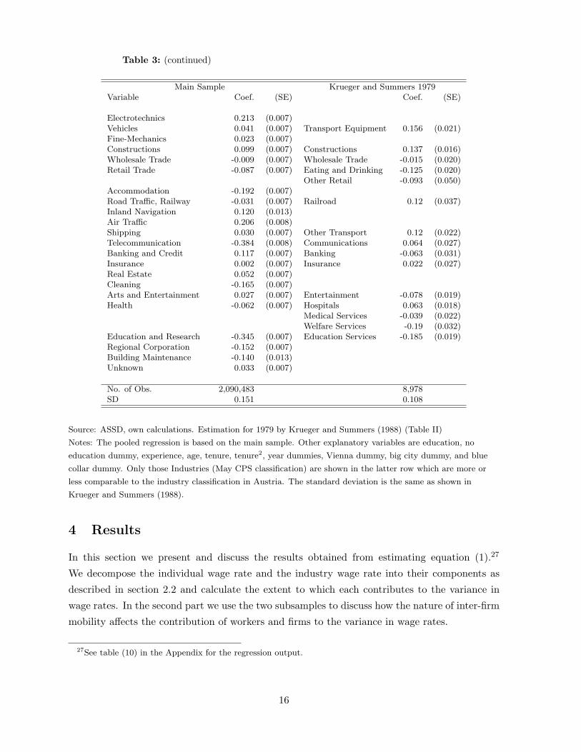
Table 3: (continued)
Main Sample Krueger and Summers 1979Variable Coef. (SE) Coef. (SE)
Electrotechnics 0.213 (0.007)Vehicles 0.041 (0.007) Transport Equipment 0.156 (0.021)Fine-Mechanics 0.023 (0.007)Constructions 0.099 (0.007) Constructions 0.137 (0.016)Wholesale Trade -0.009 (0.007) Wholesale Trade -0.015 (0.020)Retail Trade -0.087 (0.007) Eating and Drinking -0.125 (0.020)
Other Retail -0.093 (0.050)Accommodation -0.192 (0.007)Road Traffic, Railway -0.031 (0.007) Railroad 0.12 (0.037)Inland Navigation 0.120 (0.013)Air Traffic 0.206 (0.008)Shipping 0.030 (0.007) Other Transport 0.12 (0.022)Telecommunication -0.384 (0.008) Communications 0.064 (0.027)Banking and Credit 0.117 (0.007) Banking -0.063 (0.031)Insurance 0.002 (0.007) Insurance 0.022 (0.027)Real Estate 0.052 (0.007)Cleaning -0.165 (0.007)Arts and Entertainment 0.027 (0.007) Entertainment -0.078 (0.019)Health -0.062 (0.007) Hospitals 0.063 (0.018)
Medical Services -0.039 (0.022)Welfare Services -0.19 (0.032)
Education and Research -0.345 (0.007) Education Services -0.185 (0.019)Regional Corporation -0.152 (0.007)Building Maintenance -0.140 (0.013)Unknown 0.033 (0.007)
No. of Obs. 2,090,483 8,978SD 0.151 0.108
Source: ASSD, own calculations. Estimation for 1979 by Krueger and Summers (1988) (Table II)
Notes: The pooled regression is based on the main sample. Other explanatory variables are education, no
education dummy, experience, age, tenure, tenure2, year dummies, Vienna dummy, big city dummy, and blue
collar dummy. Only those Industries (May CPS classification) are shown in the latter row which are more or
less comparable to the industry classification in Austria. The standard deviation is the same as shown in
Krueger and Summers (1988).
4 Results
In this section we present and discuss the results obtained from estimating equation (1).27
We decompose the individual wage rate and the industry wage rate into their components as
described in section 2.2 and calculate the extent to which each contributes to the variance in
wage rates. In the second part we use the two subsamples to discuss how the nature of inter-firm
mobility affects the contribution of workers and firms to the variance in wage rates.
27See table (10) in the Appendix for the regression output.
16
4.1 How Important are Firms in Wage Setting?
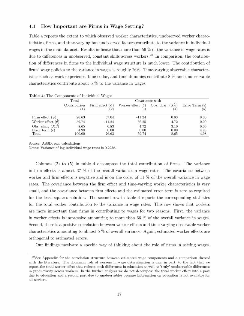
Table 4 reports the extent to which observed worker characteristics, unobserved worker charac-
teristics, firms, and time-varying but unobserved factors contribute to the variance in individual
wages in the main dataset. Results indicate that more than 59 % of the variance in wage rates is
due to differences in unobserved, constant skills across workers.28 In comparison, the contribu-
tion of differences in firms to the individual wage structure is much lower. The contribution of
firms’ wage policies to the variance in wages is roughly 26%. Time-varying observable character-
istics such as work experience, blue collar, and time dummies contribute 8 % and unobservable
characteristics contribute about 5 % to the variance in wages.
Table 4: The Components of Individual WagesTotal Covariance with
Contribution Firm effect ( �ψ) Worker effect (�θ) Obs. char. (X �β) Error Term (�ε)(1) (2) (3) (4) (5)
Firm effect ( �ψ) 26.63 37.04 -11.24 0.83 0.00
Worker effect (�θ) 59.74 -11.24 66.25 4.72 0.00
Obs. char. (X �β) 8.65 0.83 4.72 3.10 0.00Error term (�ε) 4.98 0.00 0.00 0.00 4.98Total 100.00 26.63 59.74 8.65 4.98
Source: ASSD, own calculations.Notes: Variance of log individual wage rates is 0.2238.
Columns (2) to (5) in table 4 decompose the total contribution of firms. The variance
in firm effects is almost 37 % of the overall variance in wage rates. The covariance between
worker and firm effects is negative and is on the order of 11 % of the overall variance in wage
rates. The covariance between the firm effect and time-varying worker characteristics is very
small, and the covariance between firm effects and the estimated error term is zero as required
for the least squares solution. The second row in table 4 reports the corresponding statistics
for the total worker contribution to the variance in wage rates. This row shows that workers
are more important than firms in contributing to wages for two reasons. First, the variance
in worker effects is impressive amounting to more than 66 % of the overall variance in wages.
Second, there is a positive correlation between worker effects and time-varying observable worker
characteristics amounting to almost 5 % of overall variance. Again, estimated worker effects are
orthogonal to estimated errors.
Our findings motivate a specific way of thinking about the role of firms in setting wages.
28See Appendix for the correlation structure between estimated wage components and a comparison thereofwith the literature. The dominant role of workers in wage determination is due, in part, to the fact that wereport the total worker effect that reflects both differences in education as well as ’truly’ unobservable differencesin productivity across workers. In the further analysis we do not decompose the total worker effect into a partdue to education and a second part due to unobservables because information on education is not available forall workers.
17
A candidate theory must rationalize moderate differences in firm wage policies combined with
negative sorting of workers across firms at the individual level. For instance, the theory of
equalizing differences puts forward the idea that firms’ wage policies reflect remuneration for
dis-amenities, risk of injury or death or other job characteristics (Rosen (1986)). In this view,
the firm’s contribution to the wage rate is a risk premium. Since technology differs across firms,
firm wage policies differ. Negative sorting of workers across firms occurs due to the income effect
– high wage earners ’purchase’ safer jobs (Hwang, Reed, and Hubbard (1992)).
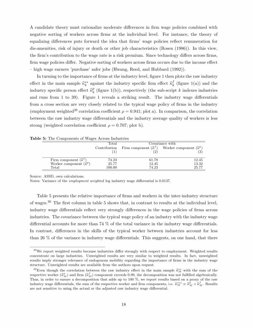
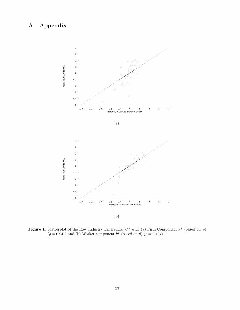
In turning to the importance of firms at the industry level, figure 1 then plots the raw industry
effect in the main sample κ̂∗∗k against the industry specific firm effect κ̂fk (figure 1(a)) and the
industry specific person effect κ̂pk (figure 1(b)), respectively (the sub-script k indexes industries
and runs from 1 to 39). Figure 1 reveals a striking result. The industry wage differentials
from a cross section are very closely related to the typical wage policy of firms in the industry
(employment weighted29 correlation coefficient ρ = 0.941; plot a). In comparison, the correlation
between the raw industry wage differentials and the industry average quality of workers is less
strong (weighted correlation coefficient ρ = 0.707; plot b).
Table 5: The Components of Wages Across IndustriesTotal Covariance with
Contribution Firm component (�κf ) Worker component (�κp)(1) (2) (3)
Firm component (�κf ) 74.23 61.78 12.45Worker component (�κp) 25.77 12.45 13.32Total 100.00 74.23 25.77
Source: ASSD, own calculations.Notes: Variance of the employment weighted log industry wage differential is 0.0137.
Table 5 presents the relative importance of firms and workers in the inter-industry structure
of wages.30 The first column in table 5 shows that, in contrast to results at the individual level,
industry wage differentials reflect very strongly differences in the wage policies of firms across
industries. The covariance between the typical wage policy of an industry with the industry wage
differential accounts for more than 74 % of the total variance in the industry wage differentials.
In contrast, differences in the skills of the typical worker between industries account for less
than 26 % of the variance in industry wage differentials. This suggests, on one hand, that there
29We report weighted results because industries differ strongly with respect to employment. Weighted resultsconcentrate on large industries. Unweighted results are very similar to weighted results. In fact, unweightedresults imply stronger relevance of endogenous mobility regarding the importance of firms in the industry wagestructure. Unweighted results are available from the authors upon request.
30Even though the correlation between the raw industry effect in the main sample �κ∗∗M with the sum of the
respective worker (�κpM ) and firm (�κf
M ) component exceeds 0.99, the decomposition was not fulfilled algebraically.Thus, in order to ensure a decomposition that adds up to 100 %, we report results based on a proxy of the rawindustry wage differentials, the sum of the respective worker and firm components, i.e. �κ∗∗s
M ≡ �κpM + �κf
M . Resultsare not sensitive to using the actual or the adjusted raw industry wage differential.
18
are systematic differences in firms’ wage policies across industries and, on the other hand, that
worker sorting across industries is much less important.
Columns (2) and (3) in table 5 decompose total contribution of firms to the inter-industry
wage structure. Across industries, average firm wage policies vary very strongly relative to the
overall variance of the industry wage structure. The inter-industry firm wage structure accounts
for more than 61 % of the overall variance. In contrast, the variance in remuneration of the
average worker across industries is about 13 % of total variance. Thus, workers differ much
less across industries than firms. Third, the correlation between the typical wage policy in the
industry with compensation for the typical worker is positive and amounts to 12 % of total
variance.
Contrasting the importance of firms for wages across individuals and for wages across indus-
tries provides a striking result. Firms are much more important in determining the inter-industry
wage structure than wage differentials across individuals. Tables 4 and 5 show that this result
is due to the fact that both the relative variance in the firm’s contribution and the covariance
with the worker’s contribution are larger at the industry level rather than at the firm level.
Larger relative variance of firm’s contribution suggests that the industry category very much
groups similar firms within industries rather than across industries (in comparison with work-
ers). Larger covariance indicates that better paying industries tend to attract workers who are
more productive.
The finding that raw industry differentials reflect primarily unobserved differences in firms’
wage policies rather than the differences in unobserved skills of workers across industries stands
in contrast to the literature. For instance, Abowd, Kramarz, and Margolis (1999b) find that the
raw industry wage differentials are virtually orthogonal to the firm component and very strongly
positively correlated with the worker component in France. The result is different for the U.S.
with firms contributing a roughly similar fraction to industry wage differentials as workers.
(Abowd, Finer, and Kramarz (1999a)) However, note that existing studies that investigated
the correlation between raw industry differentials with industry specific person and firm effects
have relied either on conditional estimation methods (Abowd, Kramarz, and Margolis (1999b);
Abowd, Finer, and Kramarz (1999a)) or did not apply the full statistical model discussed in
section 3 (Goux and Maurin (1999)). Abowd, Creecy, and Kramarz (2002) find that conditional
estimation methods may not work very well if the set of conditioning variables Z is limited.
4.2 Inter-firm Mobility
Table 6 discusses how the nature of inter-firm mobility affects the contribution of workers and
firms to the variance in wage rates. The top left cell in table 6 reports the contribution of firms
in the JTJ sample to the variance in wage rates is 26 %. In contrast, in the JUJ sample the firms’
contribution to the variance in wage rate is much higher; more than 38 % (second cell, top row).
Endogenous mobility leads to a reduction of the importance of firms in wage determination by
19
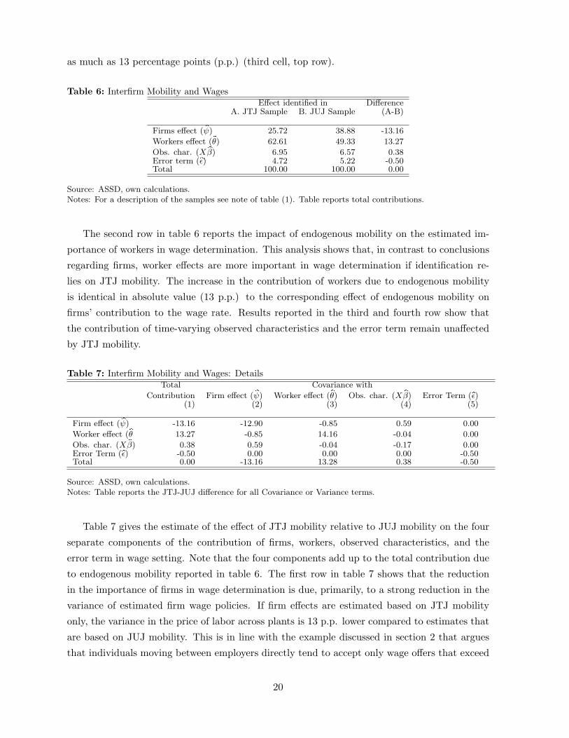
as much as 13 percentage points (p.p.) (third cell, top row).
Table 6: Interfirm Mobility and WagesEffect identified in Difference
A. JTJ Sample B. JUJ Sample (A-B)
Firms effect ( �ψ) 25.72 38.88 -13.16
Workers effect (�θ) 62.61 49.33 13.27
Obs. char. (X �β) 6.95 6.57 0.38Error term (�ε) 4.72 5.22 -0.50Total 100.00 100.00 0.00
Source: ASSD, own calculations.Notes: For a description of the samples see note of table (1). Table reports total contributions.
The second row in table 6 reports the impact of endogenous mobility on the estimated im-
portance of workers in wage determination. This analysis shows that, in contrast to conclusions
regarding firms, worker effects are more important in wage determination if identification re-
lies on JTJ mobility. The increase in the contribution of workers due to endogenous mobility
is identical in absolute value (13 p.p.) to the corresponding effect of endogenous mobility on
firms’ contribution to the wage rate. Results reported in the third and fourth row show that
the contribution of time-varying observed characteristics and the error term remain unaffected
by JTJ mobility.
Table 7: Interfirm Mobility and Wages: DetailsTotal Covariance with
Contribution Firm effect ( �ψ) Worker effect (�θ) Obs. char. (X �β) Error Term (�ε)(1) (2) (3) (4) (5)
Firm effect ( �ψ) -13.16 -12.90 -0.85 0.59 0.00
Worker effect (�θ 13.27 -0.85 14.16 -0.04 0.00
Obs. char. (X �β) 0.38 0.59 -0.04 -0.17 0.00Error Term (�ε) -0.50 0.00 0.00 0.00 -0.50Total 0.00 -13.16 13.28 0.38 -0.50
Source: ASSD, own calculations.Notes: Table reports the JTJ-JUJ difference for all Covariance or Variance terms.
Table 7 gives the estimate of the effect of JTJ mobility relative to JUJ mobility on the four
separate components of the contribution of firms, workers, observed characteristics, and the
error term in wage setting. Note that the four components add up to the total contribution due
to endogenous mobility reported in table 6. The first row in table 7 shows that the reduction
in the importance of firms in wage determination is due, primarily, to a strong reduction in the
variance of estimated firm wage policies. If firm effects are estimated based on JTJ mobility
only, the variance in the price of labor across plants is 13 p.p. lower compared to estimates that
are based on JUJ mobility. This is in line with the example discussed in section 2 that argues
that individuals moving between employers directly tend to accept only wage offers that exceed
20

the wage rate in the previous employer. This leads to a reduction in the variance of estimated
firm wage policies relative to the variance in actual firm wage policies. The third cell in the first
row of table 7 shows that the covariance between workers and firms tends to decrease slightly
due to endogenous mobility (-0.9 p.p.). Endogenous mobility increases slightly the covariance
between firm effects and observables (0.6 p.p.).
The second row in table 7 decomposes the contribution of workers to the variance in wages.
In contrast to firms, endogenous mobility leads to an increase in the variance of the worker effect
relative to the total variance in wages (14 p.p.). There is a small reduction in the covariance
between estimated worker effects and the effect of observables on the wage rate (-0.04 p.p.) and
no effect of endogenous mobility effect on the covariance between the error term and the worker
effect. Thus, as a result, the total contribution of workers to the variance in wages is higher in
JTJ mobility than in JUJ mobility estimates by more than 13 p.p.
Table 8: The Importance of Firms in Different DatasetsEffect identified in Difference
A. JTJ Sample B. JUJ Sample (A-B)
Effect used inSub-samples (A: JTJ, B: JUJ) 25.72 38.88 -13.16
(441,900) (299,310)
Common firms sample 21.91 27.49 -5.58(1,497,943) (1,497,943)
Main sample 23.09 29.10 -6.10(1,751,218) (1,721,323)
Source: ASSD, own calculations.Notes: Number of observations in parentheses. Common firms is the sub-sample for which firm effects areidentified in both the JTJ sample and the JUJ sample.
Contrasting the JTJ sample with the JUJ sample suffers from an important problem. The
fact that workers and firms differ across these two samples may by itself already drive the
conclusion that firm effects are more strongly correlated with the wage rate in the JUJ sample
than in the JTJ sample.31 Table 8 addresses this concern by reporting the importance of
31A second concern is of statistical nature. Perhaps firm effects are identified more precisely in the JUJdataset relative to the JTJ dataset. However, taking the average number of observations per firm as a proxyfor the precision of the estimates, note that firm effects will be estimated more precisely in the JTJ sample (8.1observations per firm) than in the JUJ sample (5.8 observations per firm). Nevertheless, we investigate thisissue as follows. First, we pool JTJ observations and JUJ observations. We then allocate the 123,669 workersrandomly into two datasets. The first random partition data contains the same number of workers as the originalJTJ dataset, and the second random partition dataset contains the same number of workers as the JUJ dataset.Third, we apply the wage decomposition to these two random partition sub-datasets. These datasets are similarto the original JTJ and JUJ dataset with respect to the number of workers, number of firms, and number ofobservations. In contrast to the original datasets, however, both random partition datasets are characterized byidentical shares of JTJ transitions. Results indicate that the importance of firms is 28.12 % in the ’JTJ’ randompartition data, and 27.54 % in the ’JUJ’ random partition data. This suggests that precision of the estimates isnot driving results. Furthermore, this analysis shows that the the JTJ and JUJ dataset produce results that aresimilar to the main sample when they are mixed at random. This means that focusing on sub-set movers does
21
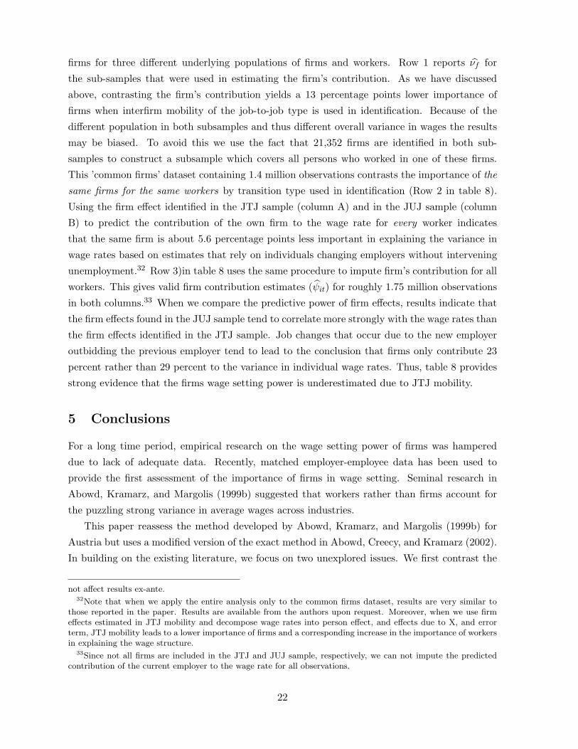
firms for three different underlying populations of firms and workers. Row 1 reports ν̂f for
the sub-samples that were used in estimating the firm’s contribution. As we have discussed
above, contrasting the firm’s contribution yields a 13 percentage points lower importance of
firms when interfirm mobility of the job-to-job type is used in identification. Because of the
different population in both subsamples and thus different overall variance in wages the results
may be biased. To avoid this we use the fact that 21,352 firms are identified in both sub-
samples to construct a subsample which covers all persons who worked in one of these firms.
This ’common firms’ dataset containing 1.4 million observations contrasts the importance of the
same firms for the same workers by transition type used in identification (Row 2 in table 8).
Using the firm effect identified in the JTJ sample (column A) and in the JUJ sample (column
B) to predict the contribution of the own firm to the wage rate for every worker indicates
that the same firm is about 5.6 percentage points less important in explaining the variance in
wage rates based on estimates that rely on individuals changing employers without intervening
unemployment.32 Row 3)in table 8 uses the same procedure to impute firm’s contribution for all
workers. This gives valid firm contribution estimates (ψ̂it) for roughly 1.75 million observations
in both columns.33 When we compare the predictive power of firm effects, results indicate that
the firm effects found in the JUJ sample tend to correlate more strongly with the wage rates than
the firm effects identified in the JTJ sample. Job changes that occur due to the new employer
outbidding the previous employer tend to lead to the conclusion that firms only contribute 23
percent rather than 29 percent to the variance in individual wage rates. Thus, table 8 provides
strong evidence that the firms wage setting power is underestimated due to JTJ mobility.
5 Conclusions
For a long time period, empirical research on the wage setting power of firms was hampered
due to lack of adequate data. Recently, matched employer-employee data has been used to
provide the first assessment of the importance of firms in wage setting. Seminal research in
Abowd, Kramarz, and Margolis (1999b) suggested that workers rather than firms account for
the puzzling strong variance in average wages across industries.
This paper reassess the method developed by Abowd, Kramarz, and Margolis (1999b) for
Austria but uses a modified version of the exact method in Abowd, Creecy, and Kramarz (2002).
In building on the existing literature, we focus on two unexplored issues. We first contrast the
not affect results ex-ante.32Note that when we apply the entire analysis only to the common firms dataset, results are very similar to
those reported in the paper. Results are available from the authors upon request. Moreover, when we use firmeffects estimated in JTJ mobility and decompose wage rates into person effect, and effects due to X, and errorterm, JTJ mobility leads to a lower importance of firms and a corresponding increase in the importance of workersin explaining the wage structure.
33Since not all firms are included in the JTJ and JUJ sample, respectively, we can not impute the predictedcontribution of the current employer to the wage rate for all observations.
22

extent to which firms are important in explaining wage differences across individuals and across
industries. Findings indicate that firms are very important in the inter-industry wage structure
rather than in the inter-individual wage structure. Whereas firms account for about three
quarters of the differences in wages across industries, only about one quarter of the variance in
individual wage rates is due to firms. In explaining this finding, we show that positive sorting
of workers across industries and negative sorting of workers across firms explains about one half
of the difference in the importance of firms at the industry and at the individual level. Second,
we discuss to what extent the two most important, yet fundamentally distinct types of inter-
firm mobility – job-to-job vs job-unemployment-job – affect the statistical decomposition of the
wage rate into a worker effect, a firm effect, and a transitory component. Results indicate that
the same firms are much less important in wage setting when identification relies on job-to-job
rather than job-unemployment-job mobility.
Our findings document the stylized facts that successful theories of the labor market need to
explain. A candidate theory must rationalize moderate differences in firm wage policies combined
with negative sorting of workers across firms with a strong role for firms rather than workers
in shaping the inter-industry wage structure and positive sorting of workers across industries.
Understanding the most important mechanisms that give rise to such differences in wage setting
across firms is thus an important topic of future research.
23
References
Abowd, John M., Robert Creecy, and Francis Kramarz (2002): Computing Person and Firm
Effects Using Linked Longitudinal Employer-Employee Data. Working paper, Cornell Univer-
sity.
Abowd, John M., Hampton Finer, and Francis Kramarz (1999a): Individual and Firm Hetero-
geneity in Compensation: An Analysis of Matched Longitudinal Employer and Employee Data
for the State of Washington. In: J. Haltiwanger, J. Lane, J. Spletzer, and K. Troske, editors,
The Creation and Analysis of Employer-Employee Matched Data, pages 3–24. North-Holland.
Abowd, John M. and Francis Kramarz (1999): The Analysis of Labor Markets Using Matched
Employer-Employee Data. In: O. Ashenfelter and D. Card, editors, Handbook of Labor
Economics, volume 3B, chapter 26, pages 2629–2710. North-Holland.
Abowd, John M., Francis Kramarz, and David N. Margolis (1999b): High-Wage Workers and
High-Wage Firms. Econometrica, 67(2):251–333.
Andrews, Martyn, Thorsten Schank, and Richard Upward (2004): Practical Estimation Methods
for Linked Employer-Employee Data. Discussion Paper 03/2004, Institut fuer Arbeitsmarkt-
und Berufsforschung.
Antel, John J. (1991): The Wage Effects of Voluntary Labor Mobility with and without Inter-
vening Unemployment. Industrial and Labor Relations Review, 44(2):299–306.
van den Berg, Gerard J. and Geert Ridder (1998): An Empirical Equilibrium Search Model of
the Labor Market. Econometrica, 66(5):1183–1221.
Booth, Alison (1995): The Economics of Trade Unions. Cambridge.
Burdett, Kenneth and Dale T. Mortensen (1998): Wage Differentials, Employer Size, and Un-
employment. International Economic Review, 39(2):257–273.
Cahuc, Pierre, Christian Gianella, Dominique Goux, and Andre Zylberberg (2002): Equalizing
Wage Differences and Bargaining Power: Evidence from a Panel of French Firms. Discussion
Paper 582, IZA.
Carruth, Alan, Bill Collier, and Andy Dickerson (1999): Inter-Industry Wage Differences and
Individual Heterogeneity: How Competitive is Wage Setting in the UK? Discussion Paper
99/14, University of Kent, Department of Economics.
Dickens, William T. and Lawrence F. Katz (1987): Inter-Industry Wage Differences and Industry
Characteristics. In: Kevin Lang and Jonathan Leonard, editors, Unemployment and the
Structure of Labor Markets, chapter 3, pages 48–89. Basil Blackwell Inc.
24
Farber, Henry S. (1999): Mobility and stability: the dynamics of job change in labor markets. In:
O. Ashenfelter and D. Card, editors, Handbook of Labor Economics, volume 3B, chapter 18,
pages 2629–2710. North-Holland.
Gibbons, Robert S. and Lawrence F. Katz (1992): Does Unmeasured Ability Explain Inter-
Industry Wage Differences? Review of Economic Studies, 59(3):515–535.
Gibbons, Robert S., Lawrence F. Katz, Thomas Lemieux, and Daniel Parent (2002): Compara-
tive Advantage, Learning, and Sectoral Wage Determination. Working Paper 8889, NBER.
Goux, Dominique and Eric Maurin (1999): The Persistence of Inter-Industry Wages Differen-
tials: a Reexamination on Matched Worker-firm Panel Data. Journal of Labor Economics,
17(3):492–533.
Groshen, Erica L. (1991): Sources of Intra-Industry Wage Dispersion: How Much do Employers
Matter? The Quarterly Journal of Economics, 106(3):869–884.
Hwang, Hae-Shin, Robert W. Reed, and Carlton Hubbard (1992): Compensating Wage Differ-
entials and Unobserved Productivity. Journal of Political Economy, 100:835–58.
Kahn, Lawrence M. (1998): Collective Bargaining and the Interindustry Wage Structure: Inter-
national Evidence. Economica, 65(2):507–534.
Kim, Dae Il (1998): Reinterpreting Industry Premiums: Match-Specific Productivity. Journal of
Labor Economics, 16(3):479–504.
Krueger, Alan B. and Lawrence H. Summers (1987): Reflections on the Inter-Industry Wage
Structure. In: Kevin Lang and Jonathan Leonard, editors, Unemployment and the Structure
of Labor Markets, chapter 2, pages 17–47. Basil Blackwell Inc.
Krueger, Alan B. and Lawrence H. Summers (1988): Efficiency Wages and the Inter-Industry
Wage Structure. Econometrica, 56(2):259–293.
Manning, Alan (2003): Monopsony in Motion: Imperfect Competition in Labor Markets. Prince-
ton: Princeton University Press.
Margolis, David N. and Kjell G Salvanes (2001): Do Firms Really Share Rents with their Workers
? mimeo, INSEE.
Mortensen, Dale (2003): Wage Dispersion: Why are Similar Workers Paid Differently? MIT
Press.
Murphy, Kevin M. and Robert H. Topel (1987): Unemployment, Risk, and Earnings: Testing
for Equalizing Wage Differences in the Labor Market. In: Kevin Lang and Jonathan Leonard,
editors, Unemployment and the Structure of Labor Markets, chapter 5, pages 103–140. Basil
Blackwell Inc.
25
Postel-Vinay, Fabien and Jean-Marc Robin (2002): Equilibrium Wage Dispersion with Worker
and Employer Heterogeneity. Econometrica, 70(6):2295–2350.
Rosen, Sherwin (1986): The Theory of Equalizing Differences. In: Orley C. Ashenfelter and
Richard Layard, editors, Handbook of Labor Economics, volume 1, chapter 12, pages 641–
692. North Holland.
Shapiro, Carl and Joseph Stiglitz (1984): Equilibrium Unemployment as a Worker Discipline
Device. American Economic Review, 75(4):892–893.
Slichter, Sumner H. (1950): Notes on the Structure of Wages. Review of Economics and Statis-
tics, 32(1):80–91.
Topel, Robert H. and Michael P. Ward (1994): Job Mobility and Careers of Young Men. The
Quarterly Journal of Economics, 107(2):439–479.
Vainiomki, Jari and Seppo Laaksonen (1995): Inter-Industry Wage Differentials in Finland:
Evidence from longitudinal census data for 1975-85. Labour Economics, 2(2):161–173.
Winter-Ebmer, Rudolph (1994): Endogenous Growth, Human Capital, and Industry Wages.
Bulletin of Economic Research, 46(4):289–314.
Zweimueller, Josef and Erling Barth (1994): Bargaining Structure, Wage Determination, and
Wage Dispersion in 6 OECD Countries. Kyklos, 47(1):81–93.
26
A Appendix
Raw
Indu
stry
Effe
ct
Industry Average Person Effect
−.5 −.4 −.3 −.2 −.1 0 .1 .2 .3 .4
−.5
−.4
−.3
−.2
−.1
0
.1
.2
.3
.4
(a)
Raw
Indu
stry
Effe
ct
Industry Average Firm Effect
−.5 −.4 −.3 −.2 −.1 0 .1 .2 .3 .4
−.5
−.4
−.3
−.2
−.1
0
.1
.2
.3
.4
(b)
Figure 1: Scatterplot of the Raw Industry Differential κ̂∗∗ with (a) Firm Component κ̂f (based on ψ)(ρ = 0.941) and (b) Worker component κ̂p (based on θ) (ρ = 0.707)
27
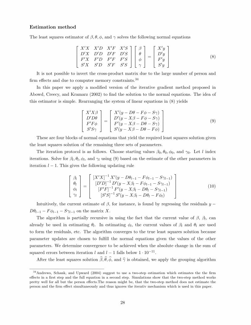
Estimation method
The least squares estimator of β, θ, φ, and γ solves the following normal equations
⎡⎢⎢⎣X ′X X ′D X ′F X ′SD′X D′D D′F D′SF ′X F ′D F ′F F ′SS′X S′D S′F S′S
⎤⎥⎥⎦
⎡⎢⎢⎣βθφγ
⎤⎥⎥⎦ =
⎡⎢⎢⎣X ′yD′yF ′yS′y
⎤⎥⎥⎦ (8)
It is not possible to invert the cross-product matrix due to the large number of person and
firm effects and due to computer memory constraints.34
In this paper we apply a modified version of the iterative gradient method proposed in
Abowd, Creecy, and Kramarz (2002) to find the solution to the normal equations. The idea of
this estimator is simple. Rearranging the system of linear equations in (8) yields
⎡⎢⎢⎣X ′XβD′DθF ′FφS′Sγ
⎤⎥⎥⎦ =
⎡⎢⎢⎣X ′(y −Dθ − Fφ− Sγ)D′(y −Xβ − Fφ− Sγ)F ′(y −Xβ −Dθ − Sγ)S′(y −Xβ −Dθ − Fφ)
⎤⎥⎥⎦ (9)
These are four blocks of normal equations that yield the required least squares solution given
the least squares solution of the remaining three sets of parameters.
The iteration protocol is as follows. Choose starting values β0, θ0, φ0, and γ0. Let l index
iterations. Solve for βl, θl, φl, and γl using (9) based on the estimate of the other parameters in
iteration l − 1. This gives the following updating rule
⎡⎢⎢⎣βl
θl
φl
γl
⎤⎥⎥⎦ =
⎡⎢⎢⎢⎣
[X ′X]−1X ′(y −Dθl−1 − Fφl−1 − Sγl−1)[D′D]−1D′(y −Xβl − Fφl−1 − Sγl−1)[F ′F ]−1 F ′(y −Xβl −Dθl − Sγl−1)[S′S]−1 S′(y −Xβl −Dθl − Fφl)
⎤⎥⎥⎥⎦ (10)
Intuitively, the current estimate of β, for instance, is found by regressing the residuals y −Dθl−1 − Fφl−1 − Sγl−1 on the matrix X.
The algorithm is partially recursive in using the fact that the current value of β, βl, can
already be used in estimating θl. In estimating φl, the current values of βl and θl are used
to form the residuals, etc. The algorithm converges to the true least squares solution because
parameter updates are chosen to fulfill the normal equations given the values of the other
parameters. We determine convergence to be achieved when the absolute change in the sum of
squared errors between iteration l and l − 1 falls below 1 · 10−11.
After the least squares solution β̂, θ̂, φ̂, and γ̂ is obtained, we apply the grouping algorithm
34Andrews, Schank, and Upward (2004) suggest to use a two-step estimation which estimates the the firmeffects in a first step and the full equation in a second step. Simulations show that the two-step method workspretty well for all but the person effects.The reason might be, that the two-step method does not estimate theperson and the firm effect simultaneously and thus ignores the iterativ mechanism which is used in this paper.
28

discussed in Abowd et al. (2002a) in order to establish the number of identified effects. We
normalize the person constant, the firm constant, and firm tenure parameter to be relative to
the mean value of this parameter within each group. Table 9 gives a summary of the results of
the grouping procedure.
Table 9: Groups and Identifiable Effectsnot Largest 2nd Largest Average of all Total of all
connected Group Group other Groups Groups
main sampleObservations 89,002 1,956,062 191 11.70 2,090,483Persons 21,560 352,716 30 2.22 378,244Firms 21,560 83,535 4 1.73 103,346Groups 1 1 11,475 11,477Identifiable Effects 436,250 33 470,113
JTJ sampleObservations 283 365,706 248 8.61 441,900Persons 88 56,251 33 1.40 68,678Firms 88 33,441 7 2.40 54,586Groups 1 1 8,822 8,824Identifiable Effects 89,691 39 114,440
JUJ sampleObservations 62 271,527 66 6.01 299,310Persons 32 49,538 9 1.18 54,991Firms 32 40,886 2 2.33 51,630Groups 1 1 4,613 4,615Identifiable Effects 90,423 10 102,006
Source: ASSD, own calculations.Note: The number of observations differs from table 1 because for some firms, the tenure slope parameter wasnot identified even though they are connected to a group. Results in the main text focus on firms with estimatesfor both entry wage φ and slope parameter γ.
We apply this procedure separately, to the main dataset, to the JTJ dataset, and to the JUJ
dataset. Thus, we end up with three sets of parameters which we index by the dataset in which
they were obtained.
29
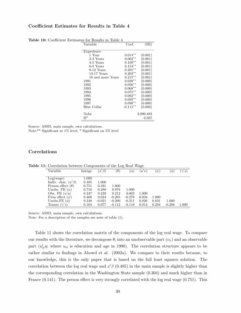
Coefficient Estimates for Results in Table 4
Table 10: Coefficient Estimates for Results in Table 4Variable Coef. (SE)
Experience1 Year 0.014∗∗ (0.001)2-3 Years 0.062∗∗ (0.001)4-5 Years 0.109∗∗ (0.001)6-8 Years 0.154∗∗ (0.001)9-12 Years 0.201∗∗ (0.001)13-17 Years 0.203∗∗ (0.001)18 and more Years 0.215∗∗ (0.001)
1991 0.039∗∗ (0.000)1992 0.056∗∗ (0.000)1993 0.068∗∗ (0.000)1994 0.075∗∗ (0.000)1995 0.092∗∗ (0.000)1996 0.092∗∗ (0.000)1997 0.098∗∗ (0.000)Blue Collar -0.115∗∗ (0.000)
Nobs 2,090,483R2 0.937
Source: ASSD, main sample, own calculations.Note:** Significant at 1% level, * Significant on 5% level
Correlations
Table 11: Correlation between Components of the Log Real WageVariable lnwage (x′β) (θ) (α) (u′ν) (ψ) (φ) (γ′s)
Log(wage) 1.000Indiv. char. (x′β) 0.485 1.000Person effect (θ) 0.751 0.331 1.000Unobs. PE (α) 0.716 0.288 0.978 1.000Obs. PE (u′η) 0.247 0.239 0.212 0.003 1.000Firm effect (ψ) 0.408 0.024 -0.265 -0.278 0.034 1.000Unobs.FE (φ) 0.348 -0.021 -0.200 -0.211 0.026 0.831 1.000Tenure (γ′s) 0.104 0.077 -0.112 -0.118 0.014 0.294 -0.288 1.000
Source: ASSD, main sample, own calculations.Note: For a description of the samples see note of table (1).
Table 11 shows the correlation matrix of the components of the log real wage. To compare
our results with the literature, we decompose θi into an unobservable part (αi) and an observable
part (u′itη; where uit is education and age in 1990). The correlation structure appears to be
rather similar to findings in Abowd et al. (2002a). We compare to their results because, to
our knowledge, this is the only paper that is based on the full least squares solution. The
correlation between the log real wage and x′β (0.485) in the main sample is slightly higher than
the corresponding correlation in the Washington State sample (0.304) and much higher than in
France (0.141). The person effect is very strongly correlated with the log real wage (0.751). This
30

finding is also present in France (0.704) but to a weaker degree for Washington State (0.511).
We find a correlation between the firm effect and the log real wage (0.408) that lies between the
results for France (0.201) and for Washington State (0.518). The correlation between the person
effect and the firm effect in Austria (-0.265) is very similar to that in France (-0.283) but more
negative than the corresponding correlation in Washington State (-0.025). Thus, results for the
main sample appear to be in line with findings in the literature. With respect to the details of
the wage policy of the firm, we note that the starting wage (φ) is negatively correlated (-0.288)
with the seniority component of the wage rate (γ′s).
31