the importance of small pelagic fishes to the energy flow ... · energy flow in marine ecosystems:...
TRANSCRIPT

Aarhus University 2010
The importance of small pelagic fishes to the
energy flow in marine ecosystems: the
Greenlandic capelin
Ph.D. dissertation
by
Rasmus Berg Hedeholm
The project was a collaboration between:
Aarhus University
The Greenland Institute of Natural Resources

Supervisors:
Associate Professor Peter Grønkjær
Department of Biological Sciences, Aarhus University
Ole Worms allé
8000 Århus C, Denmark
&
Professor Søren Rysgaard
Greenland Climate Research Centre, c/o Greenland Institute of Natural Resources
PO Box 570
3900 Nuuk, Greenland

1
Contents
Preface and Acknowledgements ....................................................................................................................... 3
Thesis structure ................................................................................................................................................. 4
List of papers ..................................................................................................................................................... 5
Dansk resumé .................................................................................................................................................... 6
English summary ................................................................................................................................................ 8
Introduction ..................................................................................................................................................... 10
Wasp-waist species and systems ..................................................................................................................... 17
Wasp-waist species and their impact .......................................................................................................... 19
Bottom-up effects.................................................................................................................................... 19
Top-down effects ..................................................................................................................................... 20
The study area ................................................................................................................................................. 22
Capelin biology ................................................................................................................................................ 25
Spawning ..................................................................................................................................................... 25
Feeding ........................................................................................................................................................ 26
Predation ..................................................................................................................................................... 27
Capelin in Greenland ....................................................................................................................................... 28
Research approach and study focus ................................................................................................................ 29
Individual studies and methods ...................................................................................................................... 31
Capelin feeding ............................................................................................................................................ 31
Capelin growth ............................................................................................................................................ 32
Capelin energy density ................................................................................................................................ 33
Capelin and Cod ........................................................................................................................................... 34
Ecopath model ............................................................................................................................................. 35
Summary of results .......................................................................................................................................... 38
Paper I: Feeding ecology of capelin (Mallotus villous Müller) in West Greenlandic waters. .................. 38
Paper II: Variation in size and growth of West Greenland capelin (Mallotus villosus) along latitudinal
gradients. ................................................................................................................................................. 39
Paper III: Energetic content and fecundity of capelin (Mallotus villosus) along a 1500 km latitudinal
gradient. .................................................................................................................................................. 39
Paper IV: Summer diet of inshore cod in West Greenland: importance of capelin. ............................... 40
Paper V: Intra-fjord variation in reproductive output in Atlantic cod (Gadus morhua). ......................... 40
Paper VI: An Ecopath model for the Nuuk fjord, Greenland. .................................................................. 41

2
Discussion and conclusions ............................................................................................................................. 44
Climate change, growth and feeding .......................................................................................................... 44
The benthic-pelagic coupling ....................................................................................................................... 47
Qualitatively changes in capelin .................................................................................................................. 48
Perspectives and future research .................................................................................................................... 51
References ....................................................................................................................................................... 53
Papers I through VI..........................................................................................................................................60
3
Preface and Acknowledgements
The present thesis “The importance of small pelagic fishes to the energy flow in marine ecosystems: the
Greenlandic capelin” has been funded by the Aarhus Graduate School of Science (AGSoS) and made in
collaboration with The Greenland Institute of Natural Resources, who have provided logistical support and
funded sampling programs. Individual projects were financially supported by the COWI foundation, the
OTICON foundation, 15. Juni foundation, Aalborg Zoo and the Augustinus fondation.
The study was performed equally at Aarhus University and at The Greenland Institute of Natural Resources
under the supervision of associate Professor Peter Grønkjær (main supervisor) and Professor Søren
Rysgaard, respectively. In addition, individual studies have been carried out in collaboration with associate
Professors Kim Mouritsen and Kurt Thomas Jensen from Aarhus University and researchers from The
Greenland Institute of Natural Resources Anja Retzel, Aqqalu Rosing-Asvid and Jonathan Carl. Also, much
appreciated assistance with sampling has been provided by employees at The Greenland Institute of
Natural Resources on various surveys, Outi Tervo and crew on RV Erika.
I wish to thank all my colleagues at Marine Ecology, especially Jens Tang Christensen and Kim Mouritsen for
helpful discussions and support. Also big thanks to fellow Ph.D. students Anders Bang, Annette Bruhn, Maja
Kjeldahl Lassen and Jens Brøgger Pedersen for encouragement and discussions. Especially, I am very
thankful to Daniel Carstensen who kept spirits high through countless hours of studying. Most importantly,
I am thankful to my supervisor Peter Grønkjær; not only for always taking the time to competently answer
my questions, but even more so for making me stick with it.
___________________________________
Rasmus Berg Hedeholm
Århus, August 2010

4
Thesis structure
In this thesis, I will present my work on the importance of small pelagic fishes in marine eocsystems. The
work has centred on the Greenlandic ecosystem and its primary pelagic species; capelin (Mallotus villosus).
Capelin was chosen as it is a key species in the ecosystem and changes in its life history can propagate to
other trophic levels. Furthermore, capelin in Greenlandic waters are relatively unstudied, inhabits a
latitudinal gradient of 17 degrees and is commercially unexploited in this area making the results unbiased
by the effects of fishery. Hence, conditions for studying the effects of temperature and spatial differences
across the species distributional range are excellent.
First, I will introduce some direct and indirect effects of climate change, especially temperature, on
marine ecosystems, the wasp-waist ecosystem concept and describe the importance pelagic organisms’
play in structuring the energy flow in such ecosystems. This is followed by an introduction to capelin in
general and its role in Greenland. The introductory text is concluded by summarizing the rationale of the
study. Second, I will present the specific scientific issues to be addressed and the methods applied. This is
followed by a summary of the major findings of the individual studies, a discussion of these and how they
have added to the current knowledge of climate effects on wasp-waist ecosystems. The specific papers will
be cited by number in accordance with the list given below and for further elaboration on methodological
and statistical procedures as well as in depth discussion of the individual studies, I refer to the articles
included at the back of the thesis. These are included in order corresponding to the introductory text and
do not reflect their chronological order.

5
List of papers
Paper I: Feeding ecology of capelin (Mallotus villous Müller) in West Greenlandic waters.
R. Hedeholm, P. Grønkjær and S. Rysgaard
Submitted to Polar Biology
Paper II: Variation in size and growth of West Greenland capelin (Mallotus villosus) along latitudinal
gradients.
R. Hedeholm, P. Grønkjær, A. Rosing-Asvid and S. Rysgaard
ICES Journal of Marine Science. doi:10.1093/icesjms/fsq024.
Paper III: Energetic content and fecundity of capelin (Mallotus villosus) along a 1500 km latitudinal gradient.
R. Hedeholm, P. Grønkjær and S. Rysgaard
Submitted to Marine Biology
Paper IV: Summer diet of inshore cod in West Greenland: importance of capelin.
R. Hedeholm, K.N. Mouritsen, J. Carl and P. Grønkjær
Prepared for submission to Journal of Marine Biology
Paper V: Intra-fjord variation in reproductive output in Atlantic cod (Gadus morhua).
R. Hedeholm, A. Retzel, S. Thomsen, K. Haidarz and K.T. Jensen
Prepared for submission to ICES journal of Marine Science
Paper VI: An Ecopath model for the Nuuk fjord, Greenland.
R. Hedeholm
Unfinished manuscript

6
Dansk resumé
I de fleste marine økosystemer ses et jævnt faldende antal af arter og individer med stigende trofisk niveau.
Visse økosystemer er dog anderledes, idet et mellemliggende trofisk niveau domineres af en enkelt meget
talrig art. Dette er typisk en planktivor fiskeart, som således er det primære forbindelsesled mellem de
lavere trofiske niveauer og top-predatorerene. Grundet denne indsnævring i energiflowet kaldes sådanne
arter for ”wasp-waist” (hvepsetalje) arter, og på grund af deres centrale placering har de afgørende
betydning for energiflowet i deres respektive økosystemer. Således kan de gennem fødeindtag begrænse
byttedyrsudbredelsen (top-down kontrol) og ligeledes begrænse fourageringsmulighederne for
prædatorerne (bottom-up kontrol). På denne baggrund er wasp-waist arternes biologi og respons på
miljøvariation yderst relevant når variation i produktion og energi omsætning skal forklares i sådanne
økosystemer.
Klimatiske ændringer vil påvirke arter og marine økosystemer på mange direkte såvel som indirekte
måder, hvilket gør det vanskeligt at kvantificere og forudsige effekten af ændringerne. På grund af deres
centrale position og strukturerende rolle, er wasp-waist arterne oplagte udgangspunkter for at adressere
potentielle biologiske konsekvenser af klimaændringer. Tilgangen til sådanne studier spænder fra
kontrollerede laboratorieforsøg til in situ indsamlede prøver. Begge er forbundet med fordele og ulemper,
men sidstnævnte tilgang har dog som forudsætning, at studieområdet er forbundet med naturligt
forekommende klimatiske gradienter. Sådan en 1500 km gradient er til stede langs den Grønlandske kyst,
hvor lodden langs hele gradienten er den dominerende wasp-waist art. Da lodden endvidere er uudnyttet i
Grønland er fiskeriinducerede økologiske effekter minimale, og området er særligt velegnet til studier af
det generelle energiflow i wasp-waist økosystemer, samt til at opnå en øget forståelse af hvilke effekter
klimatiske ændringer vil have på energiflowet i lignende systemer.
I dette studie beskrives rummelig variation i udvalgte træk af loddens livshistorie, og de relateres til de
potentielle klimatiske ændringer. Således beskrives loddens vækst ved otolith analyse, og der vises en klar
vækstforøgelse med stigende breddegrad. Dette er sammenfaldende med stigende temperaturer, og
tilsyneladende øges væksten årligt med 0,5 cm pr 1˚C temperaturstigning. En lignende breddegrads-
relateret gradient vises for loddens fødebiologi, hvor det totale relative fødeindtag stiger med breddegrad
og loddens diæt domineres i stigende grad af større og mere energetisk favorabelt bytte. Fælles for
gradienterne i vækst og fødeindtag er dog, at der længst med nord ses et fald, hvilket er sammenfaldende
med et temperaturfald. Endvidere demonstreres det, at loddens energidensitet stiger med loddens
størrelse, og desuden varierer med geografisk position og livsstadie (gydende/ikke-gydende). Sammenholdt

7
viser disse studier, at loddens biologi ændres kraftigt langs breddegradsgradienten, og man kan da forvente
en stor respons på forestående klimatiske forandringer.
Ud over disse studier af loddens biologi, præsenteres to studier, som illustrerer loddens betydning som
byttedyr. Hos torsk udgør lodden 70% af føden i sommerperioden i to Grønlandske fjorde, og det
reproduktive output (kJ) er tilsyneladende større, når torsken har øget adgang til lodde som byttedyr. Da
loddens størrelse, energiindhold og udbredelse kan forventes at ændres med temperaturforandringer, så
indikerer dette, at sådanne ændringer kan have stor betydning for såvel lavere som højere trofiske
niveauer. Loddens dominerende rolle underbygges endvidere af en samlende Ecopath model, som
implementerer den nye viden præsenteret her i en model over Nuuk fjorden, hvor allerede eksisterende
data ligeledes er indeholdt.
Dette arbejde understreger den dominerende rolle, som lodden har i det Grønlandske økosystem, hvilket
kan tages som en proxy for den generelle betydning af wasp-waist arter. Endvidere påvises det, at
klimatiske ændringer vil have en effekt på klassiske livshistorie træk såsom vækst og fødebiologi, men også
på kvalitative aspekter i form af energiindhold, Disse resultater forudsiger store ændringer i energi flow
wasp-waist økosystemer som følge af temperatur ændringer, og er et skridt imod den svære opgave det er,
at kvantificere sådanne effekter.

8
English summary
In most marine ecosystems, there is a decline in number of species and individuals with increasing trophic
level. Some ecosystems, however, differ and are dominated by very high abundance of a single species of
intermediate trophic level. This is typically a planktivorous fish species that functions as the primary
connection between lower trophic levels and top predators. Such species are called “wasp-waist species”
due to the constriction of energy flow through their central position in the ecosystems. They are of vital
importance to the energy flow in their respective ecosystems, restricting prey distribution through their
consumption (top-down control) and also limiting predator foraging possibilities (bottom-up control).
Based on this, wasp-waist species biology and response to environmental variation is integral to explaining
variability in production and energy cycling in such ecosystems.
Climate change will affect species and ecosystems in multiple direct and indirect ways, making
quantification and prediction of effects difficult. With their central position and structuring role in the
ecosystem, the wasp-waist species present an obvious starting point to begin addressing the potential
biological consequences of climate change. As such, there have been a number of studies implemented to
address climate-related questions on such keystone species with approaches varying from controlled
laboratory studies to in situ collected samples. All approaches have various advantages and disadvantages
but a prerequisite to the latter is a study area associated with naturally occurring climatic gradients. Such a
1500 km gradient is present along the Greenlandic coast with capelin being the dominant wasp-waist
species along the entire gradient. Furthermore, as capelin is unexploited in Greenland, the area is
unencumbered by fisheries-induced ecological effects and particularly well-suited to studies concerning the
natural energy flow in wasp-waist systems, as well as increasing knowledge on the possible effects of
climate change on similar systems.
In this study, spatial variability of capelin life history parameters are described in relation to potential
climate change. Capelin growth is estimated from analysis of otoliths and shown to increase with increasing
latitude. This is coincident with increasing temperatures with a 0.5 cm increase in total length for a 1˚C
temperature increase. Similarly, a latitudinal gradient was found for capelin feeding with increases in
relative prey intake and a diet increasingly dominated by more energetically favourable prey moving north.
An exception to this trend occurs in the most northerly part of the study area where there is a decline in
temperature and corresponding declines in growth and prey intake gradients. Furthermore, capelin energy
density is shown to increase with capelin size and also vary with geographical position and life stage
(spawning/non-spawning). Jointly, these studies demonstrate that capelin biology changes drastically along
the latitudinal gradient and a large response to eminent climatic change can be expected.

9
In addition to these studies on capelin biology, two studies that illustrate capelin importance as prey are
presented. For cod, capelin constitutes 70% of the prey during the summer period in two Greenlandic
fjords and there is an apparent increase in cod reproductive output with increased access to capelin prey.
Thus, capelin size, energy content and distribution can be expected to change with expected climate
change with dramatic implications to both low and high trophic levels. The dominant role of capelin is
further supported a unifying Ecopath model for the Nuuk fjord, which implements the new knowledge
presented here along with existing data.
The present work emphasizes the dominant role of capelin in the Greenlandic ecosystem and can be
seen as a proxy for the general importance of wasp-waist species. Further, the work demonstrates the
likely influence of climatic changes on classical life history traits such as growth and feeding ecology as well
as qualitative aspects such as energy density. These results predicts large changes in energy flow of wasp-
waist ecosystems following temperature changes and provide a step towards the difficult task of
quantifying such effects.

10
1988 1992 1996 2000 2004 2008
No
. o
f p
ub
lica
tio
ns p
r. y
ea
r
0
2000
4000
6000
8000
10000
12000
Figure 1: The number of publications found in a
Web of Science search using a “Climate change”
search term. The search was done on May 2nd
2010.
Introduction
Climate changes are presently the focus of much of the scientific community and have seen an accelerating
representation in the literature over the past decades since the first in Nature in 1910 (Lockyer, 1910). A
simple search in the primary literature reveals an exponential increase in the number of publications
addressing climate change (Fig. 1). This increase in scientific interest reflects the expected changes in both
global air and ocean temperatures projected in climate models and the effect it will have on biological and
oceanographic systems. The projected changes from climate models vary with modelling approach and the
area in question (Fig. 2, Meehl et al., 2007), but the majority of models project global air and ocean
temperature rises in the order of 2-4˚C and 0.5-1˚C within a millennium, respectively (Meehl et al., 2007)
with differences caused by the greater heat capacity of water compared to air. These increases would be a
further development of recent documented trends.
Hence, ocean temperatures has increased by
0.31˚C in the top 300 meters of the water column
since the 1950’s (Levitus et al., 2000) but changes
have been documented as deep as 3000 meters
(Barnett et al., 2005). However, climatic changes
will not be uniformly distributed. Hence, in the last
50 years a large part of the North Atlantic has
warmed whereas waters in southern Greenland
have cooled as a result of NAO fluctuations
superimposed on large scale patterns (Fig. 3,
Bindoff et al., 2007). This serves to underline the
complexity associated with predicting future
changes, but that changes are eminent seems beyond doubt.
In marine systems, the expected temperature changes will have both direct and indirect effects on living
organisms. Such effects include changes in productivity, distribution and feeding ecology of individual
species and in turn, such changes can alter the overall energy flow of the ecosystem. In order to understand
and predict these ecosystem changes the response of individual species to temperature changes must be
understood, and subsequently integrated in a larger context.
Focusing on fish species, the production and energetic demands are linked to the direct temperature
effect through it influence on key physiological rates such as metabolism (Sylvestre et al., 2007),
assimilation, gastric evacuation (Andersen, 2001) and gonad maturation (Hutchings and Myers, 1994),

11
Latitude (o)
Tem
pera
ture
change (
oC
)
0
2
4
6
8
Year
2000 2020 2040 2060 2080 2100
Zonal related air temperature change
Projected air temperature change
0 30oN 60
oN 90
oN30
oS60
oS90
oS
Figure 2: The solid line refers to the top axis and
shows the projected changes in air temperature
under the A2 IPCC model scenario (see reference)
in the 21st century. The line represents the mean of
the model ensemble.
The dashed line refers to the bottom axis and is
the spatial resolution of the solid line at the end of
the 21st century. Hence, it shows the projected
change in temperature at all latitudes under the
A2 IPCC model scenario. Based on data in Meehl et
al. (2007).
which result in a positive temperature-growth
relationship (Michalsen et al., 1998). However, the
increased metabolic demands imposed by
temperature increases means that such positive
effects are dependent on sufficient prey
availability and furthermore, the temperature
tolerance of individual species can entail
worsening conditions in their southern
distributional limit if the changes are not
restricted to the positive phase of the
temperature optimum curve (Fig. 4, Wootton,
1990). This was the case in Greenland cod (Gadus
ogac) along the Greenlandic West coast in the
relatively warm 1920’s and 1930’s, where a
northerly distributional shift resulted in cod
disappearance from South Greenland coincident
with an increased abundance in the north
(Nielsen, 1992 and references therein). The
positive effects of temperature are apparent
when comparing growth of Atlantic cod (Gadus
morhua) throughout its North Atlantic distribution. There is a highly elevated growth in warmer (e.g. the
Irish Sea) compared to the colder areas (e.g. Greenlandic waters) where a four year cod is five times
heavier in the former and overall, temperature explains 90% of cod growth variation (Brander, 1995).
Similar temperature effects are also evident within populations subject to yearly temperature fluctuations
which has been shown both in larvae (Otterlei et al., 1999) and adults (de Cárdenas, 1996).
Reproduction is naturally a highly fitness related trait and is subject to temperature dependent variation.
Hence, gonad development is directly linked to temperature, with higher temperatures leading to earlier
maturation on both large spatial scale (Drinkwater, 1999) and on a local scale with inter-annual
temperature variation giving rise to delayed spawning in certain years. This is seen in Newfoundland
capelin where peak spawning was delayed by two weeks over a period of 5-6 years following a colder
period (Nakashima, 1996).
In addition to these very direct effects of temperature on both growth and reproduction as well as other
metabolically dependent processes, the indirect effects are equally important although often less
12
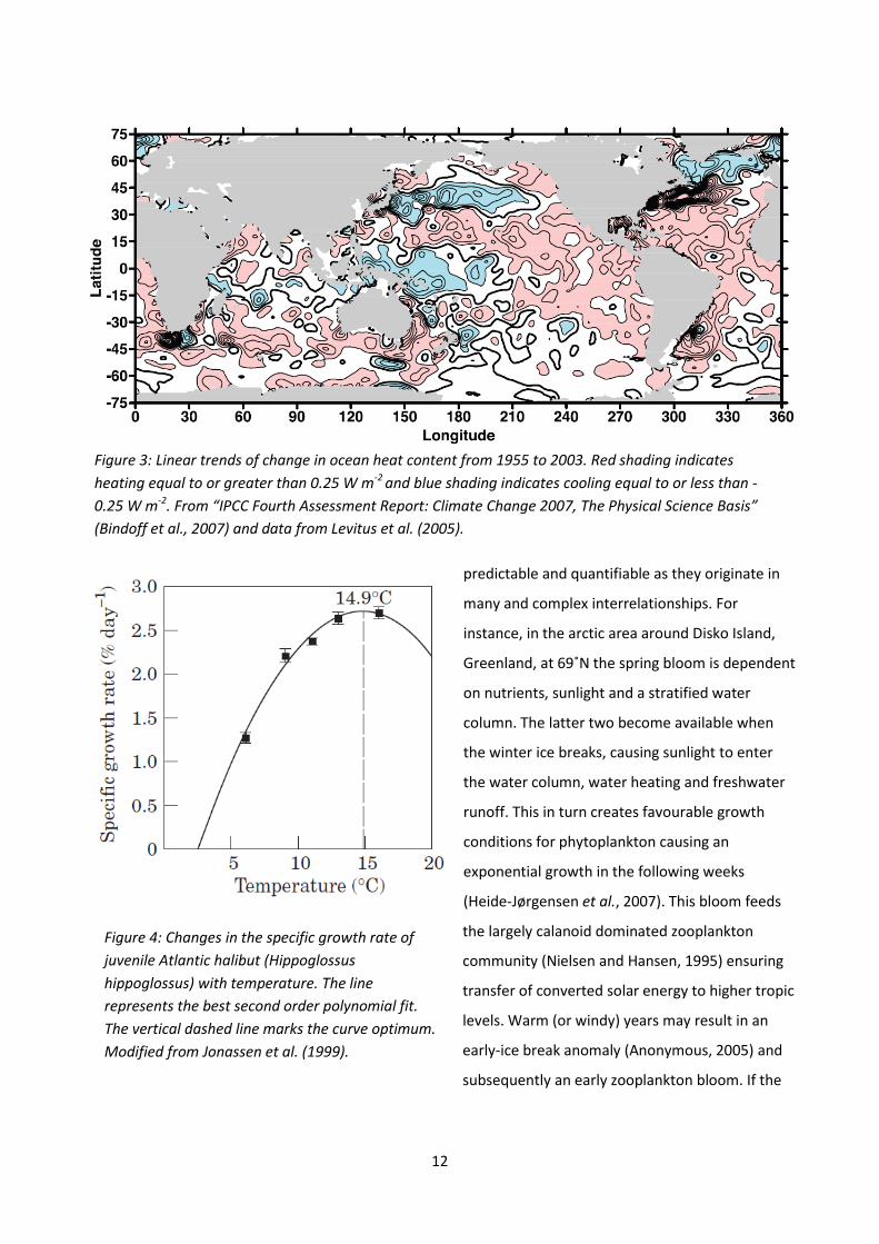
Figure 3: Linear trends of change in ocean heat content from 1955 to 2003. Red shading indicates
heating equal to or greater than 0.25 W m-2 and blue shading indicates cooling equal to or less than -
0.25 W m-2. From “IPCC Fourth Assessment Report: Climate Change 2007, The Physical Science Basis”
(Bindoff et al., 2007) and data from Levitus et al. (2005).
Figure 4: Changes in the specific growth rate of
juvenile Atlantic halibut (Hippoglossus
hippoglossus) with temperature. The line
represents the best second order polynomial fit.
The vertical dashed line marks the curve optimum.
Modified from Jonassen et al. (1999).
predictable and quantifiable as they originate in
many and complex interrelationships. For
instance, in the arctic area around Disko Island,
Greenland, at 69˚N the spring bloom is dependent
on nutrients, sunlight and a stratified water
column. The latter two become available when
the winter ice breaks, causing sunlight to enter
the water column, water heating and freshwater
runoff. This in turn creates favourable growth
conditions for phytoplankton causing an
exponential growth in the following weeks
(Heide-Jørgensen et al., 2007). This bloom feeds
the largely calanoid dominated zooplankton
community (Nielsen and Hansen, 1995) ensuring
transfer of converted solar energy to higher tropic
levels. Warm (or windy) years may result in an
early-ice break anomaly (Anonymous, 2005) and
subsequently an early zooplankton bloom. If the

13
Figure 5: All graphs reefer to the North Sea in
the period 1958 to 1999. Left: Shows the
temporal development in cod recruitment
(solid line) and the plankton anomalies
(colored legend) as determined from principal
component analysis with mean Calanus
finmarchicus abundance, calanoid size and
copepod abundance as the primary
explanatory parameters. The dashed lines
indicate the period of cod larvae occurrence
in the North Sea and the gadiod outburst
period is indicated over the graph.
Right: Mean abundance in each year of
Calanus finmarchicus and Calanus
helgolandicus (data from Continuous
Plankton Recorder, CPR). The dashed lines
indicate the period where cod larvae feed on
calanoid prey. From Beaugrand et al. (2003).
shift is large enough this could result in a classical
mismatch situation between fish larvae and their
prey (Cushing, 1975) hampering recruitment in
spite of otherwise optimal temperature
conditions. Such a mismatch situation has been
speculated to have caused a decline in Atlantic
cod recruitment in the North Sea where
alterations in inflow of water masses increased
water temperatures in the 1980’s, and caused a shift in copepod dominance from Calanus finmarchicus to
Calanus helgolandicus (Fig. 5, Beaugrand et al., 2003). The latter is temporally displaced from peak cod
larvae abundance, which causes starvation mortality in early larval stages thus hampering recruitment.
Additionally, the increased metabolic demand of the larvae associated with warmer temperatures may
prove a further disadvantage, as feeding possibilities must support the increase in demand. Hence, indirect
negative effects annul the seemingly positive effect of a temperature increase.
One possible result of the integrated effect of these direct and indirect effects is a shift in the benthic-
pelagic coupling. This entails that the supply of carbon to the benthic community is altered in either
composition (i.e. fecal pellets or phytoplankton) or quantity. Hence, if temperature effects results in an
increased pelagic biomass a larger proportion of the biomass is unavailable to the benthic community and
the biomass and/or production is reduced. In the 1960’s, changes in the North Atlantic plankton community

14
Figure 6: Based on data from 1988 to 2004 the
solid line shows the average yearly oxygen uptake
in the sediment (mmol O2 m-2 day-1, left axis) and
the dashed line shows the benthic macrofaunal
biomass (g C m-2, right axis). Redone from data in
Grebmeier et al. (2006).
caused the counter clockwise migration pattern of Norwegian spring-spawning herring (Clupea harengus)
to change (Alheit and Hagen, 1997; Loeng et al., 2005). The feeding migration was in subsequent years
restricted to more easterly waters around Svalbard and Northern Norway. Such a drastic change in
behaviour of the dominating pelagic planktivorous species can have immense impact on the structure of an
ecosystem. An abundant planktivorous species can potentially top-down control the zooplankton
community (Hassel et al., 1991; Paper VI) and the reduced grazing pressure associated with declining
herring abundance could result in a decrease in benthic production, as an increase in zooplankton
abundance would lower the supply of organic carbon to the benthic community through increased grazing
intensity. Alternatively, the increased sedimentation rate of fecal pellets compared to phytoplankton
(Taguchi, 1982; Riebesell, 1989) could increase benthic carbon supply if the slower sinking phytoplanktons
are re-mineralised during sedimentation. Hence, knowledge on water depth, water column stability, the
detritus food chain and temperature is needed to predict ecosystem response.
The possible impact of similar changes in the pelagic community has been documented in the North
Bering Sea, where conditions is conducive for a tightly coupled benthic-pelagic system (e.g. cold and
shallow) that supported a large benthic community as a result of limited grazing impact on the primary
production around the ice edge (Lovvorn et al., 2005). Climatic changes in the region, probably forced by
the Arctic oscillation, caused a shift in the community with pelagic fishes becoming more abundant as a
result of a warming trend (http://www.afsc.noaa.gov, Grebmeier et al., 2006). The higher pelagic
consumption resulted in a reduced oxygen uptake
in the sediment, indicating reduced benthic
metabolic activity and coincidently the benthic
macro faunal biomass halved (Fig. 6). At the same
time, on higher trophic levels, a spatial shift in
primary feeding grounds was observed in walrus
(Odobenus rosmarus) and grey whales
(Eschrichtius robustus). Hence, in a warming
scenario, the benthic-pelagic coupling was
apparently weakened.
A further example of the complexity of the
response of an ecosystem undergoing climatic
changes is seen in the Baltic Sea, which due to its
semi-enclosed nature is a good place to study how
interconnected the various species in a “small
Year
1988 1990 1992 1994 1996 1998 2000 2002 2004
Sedim
ent oxygen u
pta
ke (
mm
ol O
2 m
-2 d
ay
-1)
10
20
30
40
50
Benth
ic b
iom
ass (
g C
m-2
)
20
30
40
50
Oxygen uptake
Benthic biomass

15
Figure 7: The individual points and associated broken
curves reefer to herring (solid) and sprat (open) condition
(left axes) from 1986 to 2004 in the Baltic Sea. The solid
line reefers to joint clupeid abundance (right axis) in the
same period. Redone from data in Casini et al. (2006).
world” are, and how perturbations propagate in the system. In the last decades the Baltic has undergone
changes in the physical environment due to a low frequency of major inflows from the North Sea, which
has reduced salinity and oxygen content in the deeper waters, but under stable temperature conditions
(Matthaus and Franck, 1992; Møller and Hansen, 1994; Möllmann et al., 2000). This has favoured small
pelagic species herring and sprat (Sprattus sprattus), which have increased in abundance reaching very high
numbers in the mid 1990’s (Fig. 7, Casini et al., 2006). Casini et al. (2006) suggest that this apparent clupeid
success prompted increased interspecific competition which lead to a decrease in condition of both species
(Fig 7.). In addition to the effect this may have on either species’ reproductive potential (Rideout et al.,
2000) such energetic deterioration can have effects on higher trophic levels through reduced energy intake
per capita of apex predators (i.e. "The Junk Food Hypothesis", Anderson and Piatt, 1999). Such changes
have been shown to be well correlated to reduced breeding success of common guillemots (Uria aalge) in
different areas (Wanless et al., 2005; Österblom et al., 2006) and pigeon guillemot (Cepphus columba,
Litzow et al., 2002). These ecological observations have also been supported by experimental feeding trials
in for instance steller sea lions (Eumetopias jubatus, Rosen and Trites, 2000), black-legged kittiwakes (Rissa
tridactyla) and tufted puffins (Fratercula cirrhata, Romano et al., 2006). This underlines the complexity of
ecosystem response to changes not only in terms of presence and abundance, but also points to the need
for qualitative considerations in describing and predicting the effect of climatic changes. Hence, climatic
changes are to be expected in most world oceans and not least so in the North Atlantic. The effects on
fishes and ecosystems will be direct as well as indirect. How these changes will alter species distributions,
abundance, interactions and ecosystem
energy flow is not easily predictable but
already noticeable distributional shifts in
marine fishes have been seen across
species, areas and assemblages with an
estimated migration rate of several
kilometres pr. year in the current
warming period (Perry et al., 2005).
Drinkwater (2005) attempted to predict
the response of a single species by
reviewing current knowledge, which is
extensive, of temperature effects on
Atlantic cod throughout the North
Atlantic. This knowledge was used to
Year
1984 1986 1988 1990 1992 1994 1996 1998 2000 2002 2004 2006
He
rrin
g c
on
ditio
n (
g)
26
28
30
32
34
36
38
40
42
Sp
rat co
nd
itio
n (
g)
9
10
11
12
13
14
Clu
pe
id a
bu
nd
an
ce
(1
01
0 in
div
idu
als
)
0
10
20
30
40
50
Herring
Sprat
Abundance

16
Figure 8: Shows the projected changes in cod abundance following a 1˚C and a 4˚C temperature
increase, respectively. The colored dots indicate whether the changes following the temperature
increase are positive or negative. Purple and red areas show current distribution and spawning
locations, respectively. Modified from Drinkwater 2005.
project changes in abundance and distribution of cod under different climate scenarios (Fig. 8). It is clear
that cod can be expected to extend its distribution northwards and supposedly at the same time
disappearing from southern areas such as the British Isles because of ocean warming. However, even as
cod is one of the most studied species, Drinkwater (2005) still makes these predictions without including
the effect of fishing and also emphasizes: “that future changes to cod will also depend on the changes to
other parts of the ecosystem” especially with regards to the important parameter of larval feeding
possibilities, being crucial to ensure successful recruitment (Sundby, 2000). Adding to this statement, is the
presence of cod in Danish waters during a warm period between 7000-3900 BC (Enghoff et al., 2007) were
cod should not have been present given their present day phenotypic response to high temperatures.
Enghoff et al. (2007) point to genetic adaptation, migration and/or phenotypic plasticity as possible
explanations, but also mention the effect present day fishery may have on these factors. Add to this some
of the indirect effects mentioned here, it is clear that to be able to predict and understand the effects of
climatic changes to fishes and ecosystems, extensive knowledge on not only fishes, but on all aspects of the
ecosystem and the way in which they are related, is needed.
In the following, I will introduce wasp-waist systems in general, the study area and the approach applied
in the present study.

17
Wasp-waist species and systems
Most marine ecosystems consist of a multitude of species from primary producers to top predators. This
also includes from one to several pelagic fish species that often possess some shared characteristics that
include schooling behaviour, planktivorous diet, great abundance, high mobility and short life cycles.
Examples of such planktivorous pelagic fish can be found in all major water bodies and include anchovies,
sardines, herring, sprat, menhaden, atlantic silverside, capelin and sandeels. Their distinct characteristics
make these species very dynamic with a high production and capable of having a large impact on other
trophic levels. Their mobility and high energetic need (because of their numbers and high growth rates)
force them to find and subsequently exert a high predation pressure on the zooplankton community in
order to sustain the population. This makes the pelagic fish the primary converters of planktonic energy
resources to fish biomass. This also entails, that ecosystem stability and energy flow are very much affected
by these species and any environmental changes that might influence their abundance, production,
distribution and feeding ecology.
The most common structure of marine systems is one with great species diversity at the lowest trophic
levels (primary producers) and a subsequent decrease in both species and abundance with increasing
trophic level. This loss in diversity and biomass is often explained by an energy transfer efficiency of only
10% between trophic levels caused by respiratory losses, unassimilated consumed food and unconsumed
food (Pauly and Christensen, 1995). However, in many highly productive marine ecosystems across all
latitudes such as upwelling zones (e.g. South American coast) and shelf areas (e.g. West Greenland) across
all latitudes the pattern differs. Here, an intermediate trophic level is dominated by one (or a few) pelagic
species (Rice, 1995); usually small planktivorous fishes (Cury et al., 2000). As these fish are the sole species
on their trophic level, all available energy generated by the primary producers has to pass through them to
become available to predators. Hence, the planktivorous fish become important both as predator (top-
down control) and prey (bottom-up control) in the system and are often considered key stone species with
a high number of linkages within the system. Such systems containing an intermediate, energy mediating,
abundant species capable of having an influence on both lower and higher trophic levels (top-down and
bottom-up from the middle) are referred to as wasp-waist systems, inspired by the crucial connecting link
that both the pelagic species and the petiole in wasps constitute in their respective systems (Rice, 1995).
Wasp-waist system can by systematically depicted as in Fig. 9 (right), where the waist species by virtue of
their abundance and dominance of their intermediate trophic level ensures all transfer of energy from
lower to higher trophic levels. This is of course an extreme case. Many of the higher predators will feed on
levels below the waist species, at the very least in the juvenile stages as an ontogentic shift in diet is the

18
Figure 9: Two simplified food webs. Left: a food
web with no dominating wasp-waist species
connecting lower and higher trophic levels. Right:
a food web with a single abundant wasp-waist
species that transfer all energy from low to high
trophic levels. Based on Jórdan (2005).
general rule in predatory fishes (Wootton, 1990).
Furthermore, larval stages of top predators are
themselves subject to predation from many
species (e.g. Köster and Möllmann, 2000).
Due to their key position in the system, wasp-
waist species expectedly have a large influence on
other components of the system. This importance
has been demonstrated theoretically by Jordán et
al. (2005), who created ten hypothetical systems
with varying degree of waistedness (i.e. more or
less connections circumventing the waist species)
and calculated the importance of each species to
the rest of the system in all cases. They found that
a higher waistedness was associated with higher
system dependency on changes in the wasp-waist
species. This seemingly introduces potential yearly cascadal effects into the system caused by the highly
variable year-class strength of wasp-waist species. However, the stability of the system is ensured by a built
in system redundancy, owing to the massive abundance of the wasp-waist species, which dampen external
influences on the system (Jordán et al., 2005). Naturally, decreasing abundances will over longer time
periods have large effects as seen in Canadian waters, were the disappearance of capelin has been
speculated to be the proximate cause of the continued depressed state of the cod population (Rose and
O'Driscoll, 2002). The contrast to such an extremely waisted system is a system where the number of
connecting nodes between species creates the same stability (Fig. 9, left). Here, the interdependency
between species is low making no single species crucial and changes are diluted in the system by diet
switching. The North Sea could serve as an example, with its multiple planktivorous species (i.e. sprat,
herring, sandeel, Norway pout etc.) creating many energy flow pathways from bottom to top.
Reviewing wasp-waist systems across all oceans Bakun (2006) suggests that wasp-waist species possess
four characteristics that together make them the hub of their respective ecosystems and explain the
theoretical importance, which goes further than simply being a mediator of changes across trophic levels.
In summary, these are
1. Complex life histories (e.g. short-lived, pelagic larvae). This makes the waist populations vulnerable
to environmental fluctuations giving large inter-year variation.
19
2. The species dominate their trophic level which will make changes propagate to other trophic levels
because no antagonistic change is seen in similar species on the same trophic level. Hence, bottom-
up and top-down controls are realistic scenarios.
3. They are the lowest mobile trophic level. This enables wasp-waist species to follow prey items thus
forcing changes in the spatial distribution of predators and trophic interactions of the system.
4. They can predate heavily on egg and larval stages of top predators forming a negative feedback
loop in some systems that keep them abundant while suppressing that of piscivorous predators (i.e.
the “predator pit”).
Wasp-waist species and their impact To address possible effects of climate change mediated through the wasp-waist species on other trophic
levels, the issue can be simplified by focusing on the one-to-one interactions between wasp-waist species
predators (bottom-up) and prey (top-down).
Bottom-up effects
A species or trophic guild must have a controlling influence in higher trophic levels for bottom-up effects to
be present. Such an importance of small pelagic fish as prey is well documented. For example, in Icelandic
waters capelin is the main single prey item for Atlantic cod making up 50% of the prey, and in the capelin
spawning season this number reaches 80-90% (Vilhjalmsson, 2002) similar to numbers also seen in
Greenland (Paper IV). Similarly, in the Baltic Sea the main prey of cod is sprat and herring which together
make up approximately 70% of yearly averaged cod diet (Harvey et al., 2003; Österblom et al., 2006). In
seabirds, the importance of pilchard (Sardinops ocellata) and anchovy has been shown for cape cormorant
(Phalacrocorax capensis) and jackass penguin (Spheniscus demersus) in South African waters (Crawford and
Shelton, 1978) and marine mammals such as seals and whales also feed heavily on pelagic fish (Wathne et
al., 2000; Witteveen et al., 2006).
Wasp waist species are short lived (generation time from 1-4 years) and hence, they respond quickly to
biotic and abiotic changes giving large yearly variations in abundance. This was seen in Barents Sea capelin
where a 12 fold increase in 1990 (0.23 to 3.18 mio. tonnes) was followed in 1993 by a severe reduction of
80% (3.93 to 0.84 mio. tonnes, Gjøsæter et al., 1998). This large inter-year abundance variability in
connection with the predator’s dependency of one or a few prey species seemingly renders predators
highly vulnerable to such fluctuations. However, these changes do not necessarily propagate to higher
trophic levels. The system redundancy caused by waist species abundance mentioned above is one aspect
of this, but a predator lag-phase is also present due to the longer generation times generally seen at the

20
higher predatory trophic levels. This allows for a buffer effect of wasp-waist communities where the effect
of oscillations of waist species abundance are dampened (Bakun, 2006). Cury et al. (2000) mention two
examples of such delayed effects where predatory fish populations suffer severe declines a few years after
the collapse of their main pelagic fish prey, illustrating both the bottom-up effect and the inherent lag-
phase of the predator populations. Hence, the snoek (Thyrsites atun) and chub mackerel (Scomber
australasicus) collapsed two and four years after their prey, chilean anchoveta (Engraulis ringens) and
round sardinella (Sardinella aurita), respectively, suffered severe population declines (see Cury 2000 for
other examples). However, had the pelagic wasp-waist species rebounded within a couple of years the
predator population would probably have avoided the collapse. Supporting this is the simple fact that
predator population continue to survive without extreme population fluctuations in spite of ongoing prey
availability variation.
Top-down effects
That planktivorous fish prey on zooplankton does not automatically entail top-down control. In order for
top-down control to become an issue, the planktivorous fish must exert a predation pressure that limits the
abundance of zooplankton, creating an - for now disregarding the many other variables that have a
considerable influence on zooplankton abundance – inverse relationship between planktivorous fish and
zooplankton abundance. If the zooplankton is present in abundance, the planktivorous fish become
satiated and no such relationship exists.
That planktivorous fish do indeed consume a lot of energy and thus prey heavily on zooplankton has
been shown among others by Jarre-Teichmann and Christensen (1998) who estimated that in four major
upwelling systems 15-30% of the primary production is required (mediated by zooplankton) to support the
pelagic fish production. Similarly, Arrhenius (1997) estimated that herring consumed 30-60% of all
zooplankton in the Baltic and Arrhenius and Hanson (1993) showed through bioenergetic modelling of the
same system that together herring and sprat were capable of consuming as much as 80% of the
zooplankton. However, they also showed that the model was sensitive to small perturbations (i.e. 5%) in for
instance larval fish survival, which is common. For the Baltic, it has also been suggested that intense
predation can cause behavioural changes in the zooplankton community such as intensified vertical
migrations (Arrhenius, 1997) suggesting another aspect of the top-down control mechanism.
Clear top-down causal relationships are not common in the literature. This can be due to rarity of the
phenomenon, but can also be explained by the extensive sampling needed to test hypotheses and the
many other variables influencing species abundance. These include oceanographic variation, fisheries,
density dependent processes, spatial and temporal overlap (Möllmann and Köster, 2002) explaining why
clear cascadal-like relationships are not the general rule. However, there are some studies showing very

21
Figure 10: Relative changes in abundance of cod,
capelin, zooplankton and phytoplankton. White
bars represents the period prior to the 1990’s and
black bars during the 1990’s. Redone from
Carscadden (2001).
Figure 11: The relative changes in surface
chlorophyll a concentration (green line), macro
zooplankton mean weight (black line) and Pink
salmon catch per unit effort (CPUE, blue line) from
1985 to 1994 in the North Pacific (approximately
50˚N). Based on data in Shiomoto et al. (1997).
convincing data. In the Canadian West Atlantic,
environmental changes induced a southwards
shift in capelin distribution and at the same time,
cod (and other capelin predators) collapsed in the
area releasing capelin from its main predators.
This resulted in an increase in capelin abundance
which supposedly brought with it a top-down
control on zooplankton and subsequently
phytoplankton abundance in reciprocal
relationships consistent with a trophic cascade
(Fig. 10, Pace et al., 1999; Carscadden et al.,
2001). Similarly, Shiomoto et al. (1997)
demonstrated that the primary productivity in the
Northern Pacific fluctuated on a yearly basis in
spite of environmental conditions being similar between years. The phytoplankton fluctuations were
mirrored in zooplankton but with one year temporal displacement suggesting a causal relationship (Fig. 11).
This apparent top-down regulation was supposedly caused by pink salmon (Oncorhynchus gorbuscha)
which accordingly displayed a pattern of inverse
abundance with macrozooplankton. This was
most clear towards the end of the study period
(1990-1994) where salmon catch-per-unit-effort
(CPUE) indicated a sufficiently large population
capable of predating heavily upon the
macrozooplankton community. Both these studies
underline, that top-down regulation is only a valid
notion when prey abundances are indeed limited
by predation, and not only if a prey is important to
one/more predators. Thus, it appears that a top-
down effect of zooplanktivorous fishes is present
across oceans although subject to inter-year and
strength variability (Cury et al., 2000).
cod capelin zooplankton phytoplankton
Re
lative
abu
nd
an
ce
0
1
2
3
4
5
Year
1985 1986 1987 1988 1989 1990 1991 1992 1993 1994
Re
lative
va
lue
0
10
20
30
40 Chl. a concentration
Zooplankton weight
Pink salmon CPUE

22
Figure 12: The entire lengths of the lines represent
the length of the growth season at various
latitudes along the east coast of North America.
The growth season is defined as the period from
the onset of Atlantic silverside spawning to the
start of winter migration or when temperatures
dropped below 12˚C. The thick segment of the
lines is the length of the spawning season as
determined from reports of ripe adults. Based on
Conover and Present (1990).
Figure 13: The southern part of Greenland with
arrows indicating dominating currents. The
darkest arrows flowing from the north is the cold
low-saline water of polar origin and the light grey
arrows indicate high saline warmer water from
the south. These mix along the West coast of
Greenland (dark grey arrows).
Month
2 3 4 5 6 7 8 9 10 11 12
Latitu
de (
oN
)
30
32
34
36
38
40
42
44
46
The study area
Greenland has an unbroken north-south oriented coastline extending 2300 km from 60˚N to 78˚N, which is
naturally associated with gradients of ecological relevance in a climate related study. Due to the latitude
and extent of the gradient, there is a large difference in solar irradiance from south to north as the period
with sunlight and ice-free conditions becomes progressively shorter moving north thereby limiting the
growing season (Sejr et al., 2009). Because the spring phytoplankton bloom is dependent on the sunlight
and the stratification it initiates (Hansen et al., 2003) this gradient creates similar temporal differences in
the start of spring production and causes a temporal displacement of processes dependent on the bloom.
Such timely displacement is, however, not restricted to the lowest trophic levels. For instance, in North
America the result of a shorter growing season is reflected in the spawning behaviour of Atlantic silverside
(Menidia menidia) which is delayed by two months covering a 14˚ latitudinal gradient and also shortened
significantly (Fig. 12). Similarly, capelin in Greenland shows the same progressing spawning pattern over a
similar distance although less well described (Friis-Rødel and Kanneworff, 2002). Another parameter that
also varies with latitude, and often covaries with length of the growth season, is temperature. Indeed, this
covariance is one of the main problems when studying certain latitudinal related patterns, as it is difficult to
separate their joint effects on for instance growth patterns or onset of spawning. The usual pattern is that

23
Figure 14: Average temperatures from 20-50 m averaged from 1908-2007 for West Greenland shelf
waters (60˚N-73˚N and 44˚W-57˚W). Top left: data from all months and years. Top right: data for July.
Bottom left: data for August. Bottom right: data for September. Error bars represent standard error
based on the mean values of all years at given latitudes. The areas where capelin were sampled for
several of the included studies are noted at their respective latitude. Based on data from the ICES
database.
Te
mp
era
ture
(oC
)
0
1
2
3
4
Latitude (oN)
60 62 64 66 68 70 72
Te
mp
era
ture
(oC
)
0
1
2
3
4
Latitude (oN)
60 62 64 66 68 70 72
All months July
August September
Qa
qo
rto
q
Nu
uk
Dis
ko
Uu
mm
an
na
q
Qa
qo
rto
q
Nu
uk
Dis
ko
Uu
mm
an
na
q
of lower temperatures at higher latitudes. This may be true for air temperatures, but the pattern on the
West Greenland shelf and near-coastal waters is more complex. The water masses in this area are a mix of
two bodies of water (Fig. 13). From the north, flowing along the East coast of Greenland is a cold, low
salinity current. From the south a small part of the Gulf Stream, the Irminger current, flows south of
Iceland. This water is warmer and has a higher salinity (Ribergaard et al., 2008). Hence, when the two water
masses flow up the West coast of Greenland, the warm water is situated below the cold water. The water
masses gradually mix causing a heating of the surface water moving north. Around Disko Island at 69˚N, the
current has weakened and it breaks off into the Davis Strait causing a gradual cooling of the surface water
further north. This is the case both when considering the yearly average, but even more pronounced in the

24
summer months, which is the primary growth season (Fig. 14). The growth pattern of various species in
Greenlandic waters reflects these spatial differences in temperature regime. Hence, benthic organisms
such as Greenland halibut (Reinhardtius hippoglossoides, Sünksen, 2009) and sea urchin (Strongylo-
centrotus droebachiensis, Blicher et al., 2007) show a decreased growth rate with latitude in accordance
with Bergmann’s rule (Lindsey, 1966) as ambient bottom temperatures in both cases display the expected
pattern of a negative latitudinal relationship. Contrastingly, capelin, a pelagic species, displays the opposite
pattern of increased growth with latitude consistent with the warming surface waters (Paper II).
Due to the extensive unbroken north-south gradient, the expected impact of climate change in the arctic
and sub-arctic region and the many processes at all trophic levels that will be greatly affected by an altered
climate, Greenland offers a perfect platform to study the possible effects of climate change. This is both in
terms of local change where basic life history parameters such as spawning, growth rate, metabolism and
maturity can be expected to change for a number of organisms, but also on a larger scale where the
distributional pattern, spawning areas, community composition, spring bloom initiation, freshwater inflow
and benthic-pelagic coupling can be expected to change affecting the ecosystem energy flow. Many aspects
of the Greenlandic ecosystem have not been studied, although recent years have seen initiatives on
especially lower trophic levels including monthly monitoring programs (Jensen and Rasch, 2008). However,
much research on all ecosystem levels is still needed to understand interrelationships and predict upcoming
changes. Recognizing logistic, economical and timely limitations this leaves the question of which part of
the ecosystem to study to progress ecosystem understanding the furthest.
In highly connected food webs (Dunne et al., 2002) the obvious point of interest is the central part of this
food web as changes here would most directly affect the highest number of other species through top-
down and bottom-up processes. As for the arctic region in general the Greenlandic ecosystem is dominated
by relatively few species (Roy et al., 1998; Allen et al., 2002). Additionally, the Greenlandic ecosystem
displays typical wasp-waist system characteristics, with capelin functioning as the key species (Rice, 1995).
Hence, to increase knowledge on sub-arctic ecosystems under climatic influence and wasp-waist systems in
general, this study has focused on the Greenlandic capelin as it serves as the natural point of interest and
any climatic changes imposed on this key species could have cascading effects on the ecosystem through
top-down and/or bottom up processes.

25
Figure 15: Left: The distributional range of capelin. Green indicates common presence while yellow is
rare occurrences (Vilhjálmsson, 1994). Right: male (top) and female (below) capelin with clear sexual
differences in the spawning season.
Capelin biology
Many good reviews have been written on capelin biology, especially Icelandic, Barents Sea and Canadian
stocks (Gjøsæter, 1998; Carscadden et al., 2001; Vilhjalmsson, 2002), and only a brief summary is given
here.
Capelin is a small silvery member of the Osmeridae family with circumpolar distribution (Fig. 15). It
reaches different sizes at different locations but has a maximum size of 25 cm (TL, Fishbase 2008) with the
males growing the fastest but not reaching the same age as the females. Capelin has been fished in
Icelandic, Canadian and Norwegian waters with yearly catches occasionally exceeding 2 mio. tonnes (FAO -
Fisheries and Aquaculture Information and Statistics Service) making the species commercially important in
some fisheries. However, the largest fishery, the Icelandic, has in the last decade been reduced to one
tenth of previous catches and current total allowable catch is recommended at 0 tonnes due failing
recruitment (Anonymous, 2010).
Spawning Capelin spawning occurs during the summer months and usually takes place at a few meters depth
(sometimes on the beach) but demersal spawning at more than 50 meters is also seen (Kanneworff, 1967;
Vilhjálmsson, 1994; Nakashima and Wheeler, 2002). Spawning events are triggered by a multitude of
environmental factors (grain size, beach orientation, tide, waves, lunar cycle etc.) but their relative
importance is poorly understood although temperatures from 2-10˚C seems to be preferred (Vilhjálmsson,
1994; Therriault et al., 1996). Prior to spawning a sexual dimorphism develops (Fig. 15), with male pelvic,
anal and pectoral fins becoming enlarged and two ridges of enlarged scales form just above the lateral line

26
and ventrally. These function as “holders” of the female during spawning events as the male(s) lie on either
side of the female fertilizing the eggs. Fecundity is 6000-12000 and the eggs are 0.5mm (Huse and
Gjøsæter, 1997; Tereshchenko, 2002, Paper III) with an incubation time of approximately 120 degree days
(Gjøsæter, 1998). Spawning capelin are usually 3-5 year old with the biggest fish in each cohort spawning
first (Kanneworff, 1967; Vandeperre and Methven, 2007). There has been some debate over the fate of
spent individuals. That males experience very high post-spawning mortality seems to be accepted
(Vilhjálmsson, 1994; Friis-Rødel and Kanneworff, 2002; Christiansen et al., 2008) although Nakashima
(1992) found through tagging that some spawning males returned the next year. Females are supposedly
iteroparous and may survive spawning but it is not known to what extent (Kleist, 1988; Vilhjálmsson, 1994;
Flynn et al., 2001). Estimates range from survival rates of 5-50% and in some cases functionally 0% as
predation on spent females is high. Theoretically, the most profitable strategy (semelparity vs. iteroparity)
is dependent on mortality pattern in the environment. Hence, high adult mortality favours semelparity
while high/variable juvenile mortality is an incentive for iteroparity (Orzack and Tuljapurkar, 1989;
Christiansen et al., 2008). Based on these assumptions and on knowledge on capelin life history, Huse
(1998) showed through modelling that such a sex-specific life strategy theoretically maximizes reproductive
output in capelin which is also consistent with laboratory studies (Christiansen et al., 2008).
Feeding Capelin are planktivorous with 0-group capelin feeding mainly on copepodites, copepod eggs,
phytoplankton, small euphausiids and other small prey items (Pedersen and Fossheim, 2008) that are
probably chosen based on size appropriateness (Gjøsæter, 1998). The diet of older capelin is dominated by
three main food groups: copepods (mainly Calanus), euphausiids (krill) and amphipods in order of
importance and it appears that copepods are dominant at the smaller sizes while an increase in capelin size
is followed by an increase in krill consumption (Huse and Toresen, 1996; O'Driscoll et al., 2001; Orlova et
al., 2002; Paper I). Occasionally, eggs and fish larvae (including cannibalism) are consumed (Gerasimova,
1994).
In some areas the entire population undertake feeding migrations, for instance in Iceland where feeding
takes place north of Iceland and is followed by a spawning migration to the south (Vilhjalmsson, 2002). The
same is seen in Canadian (Nakashima, 1992; O'Driscoll et al., 2001) and Barents sea populations (Gjøsæter,
1998). In Greenland the populations in separate fjords are believed to stay in or very close to the fjords for
feeding as well as spawning (Friis-Rødel and Kanneworff, 2002) but capelin are caught in surveys on the
near coastal banks (K. Sünksen, Greenland Institute of Natural Resources, Pers. comm.) suggesting at least
some migration and feeding outside the fjord.

27
Predation Capelin is an important prey to many species and must be considered good quality prey due to its high
energy content of approximately 21 kJ g-1 dry weight compared to for instance pollock and cod which are
much leaner (approximately 16 kJ g-1 dry weight; Van Pelt et al., 1997; Paper III). It is the main prey of many
commercially important fish (e.g. cod, salmon), marine mammals (e.g. seals, whales) and seabirds (e.g.
common murre). Especially the cod-capelin interaction has received much attention, as capelin is the main
prey item of commercially important cod in many waters (Vilhjálmsson, 1994; Bogstad and Gjøsaeter, 2001;
Carscadden et al., 2001; Paper IV). Hence, Vilhjálmsson (2002) estimated the total annual consumption of
all capelin predators (13 species in total of fish, whales and birds) in Icelandic waters to be 2-3.8 mio.
tonnes (Vilhjálmsson 2002 and references therein) roughly equivalent to one third of the population.

28
Capelin in Greenland
Even though capelin has been studied for many years from different perspectives not many studies focus
on the Greenlandic capelin. Friis-Rødel and Kanneworff (2002) reviewed the available literature and since
then, besides the work presented here, only one article including Greenlandic capelin has been published
concerning the evolutionary origin of capelin populations (Dodson et al., 2007). The conclusions made by
Friis-Rødel and Kanneworff (2002) are however often based on assumptions and circumstantial evidence.
The best-documented conclusions concern distribution, size-at-age and spawning behaviour along the
Greenlandic coast. Capelin are distributed from Cape Farewell in the south (60˚N) to Umanak (73˚N) and
Illorqqortoormiut (70˚N) in the north on the west and east coast respectively with the northern limit
shifting with altering temperatures (Hansen, 1943; Friis-Rødel and Kanneworff, 2002). Maximum age and
length increase towards the north and the females are the larger sex at a given age although very little is
known about the actual growth pattern (Friis-Rødel and Kanneworff, 2002, Paper II)
Known differences between areas such as maximum length, progressive spawning and well separated
fjord systems suggests that individual fjord systems may contain separate stocks. This hypothesis is
supported by Sørensen and Simonsen (1988) who used proteins and gel electrophoresis to demonstrate
differences among three areas on the Greenlandic west coast. However, the number of stocks, their
distribution and total stock size is unknown although a few local biomass estimates exists (Jákupsstovu and
Røttingen, 1975; Bergstrøm and Vilhjálmsson, 2006). The feeding behaviour of capelin in Greenlandic
waters has only been briefly and superficially addressed in two master theses (Kanneworff, 1967; Kleist,
1988). Sampling has been sporadic since 1906, no new research on the ecological role of Greenlandic
capelin has been done since 1988 and since then sampling has been non-existent apart from capelin
sampled on the first day of spawning in the Nuuk fjord system.
29
Research approach and study focus
In the present study, the overall aim is to provide knowledge on the role of small pelagic fishes in wasp-
waist ecosystems, with special focus on the role they play in energy transfer and expected changes
following a temperature change. Recognizing that an entire ecosystem is not explainable from a single
study or species, the challenge is to select the approach most likely to reveal most information about the
system and any species of particular interest. The present work has been conducted from a “changing
climate” perspective and possible approaches span from controlled experimental designs with a minimum
of realism (Conover and Present, 1990) to the inverse situation of realistic but uncontrolled in situ sampling
(Sünksen, 2009) and theoretical (speculative) modelling of possible changes (Drinkwater, 2005). The in situ
sampling offers data that represent the actual situation in space or time, but also offers the challenge of
suggesting a clear causal relationship when faced with many influential parameters, which may not even
have been recorded. Ideally, the laboratory approach should be used to validate or test specific hypotheses
generated by the more holistic ecosystem approach (Conover and Present, 1990) but the appropriate
approach is naturally dependent on the study area and issues addressed.
I have chosen to focus on capelin in the Greenlandic ecosystem as a model species using a field-based
and ecosystem approach, as vital capelin parameters are lacking in this area. Capelin distribution along an
unbroken latitudinal gradient in West Greenlandic waters offers a unique chance to study a wasp-waist
system with little impact from fishing and with a natural climate gradient covering the entire distributional
range of capelin. In order to describe and to some extent quantify the importance of capelin, knowledge on
consumption rates, production, biomass, predator-prey relationships, spawning behaviour and how these
parameters are related to temperature is needed. Although many of these temperature dependent
processes are also well suited for laboratory testing, the lack of basic knowledge and logistical challenges
associated with obtaining live specimens (eggs, larvae and adults) resulted in an ecosystem based approach
and subsequently in situ sampling procedures. In some cases, logistical limitations further dictated sampling
procedures and consequently the studies focused mainly on capelin older than two years-of-age.
Substantial knowledge is needed to fully understand the role of capelin within the ecosystem, and the
present work only allows for certain aspects of capelin ecology to be addressed. First, I have chosen to
explore the naturally occurring latitudinal gradient concerning fundamental capelin traits, namely feeding
(Paper I) and growth (Paper II) as these are essential in quantifying capelin importance and are often
temperature dependent. Second, I explore the effect of latitude on capelin energy density and fecundity,
which will affect capelin quality as prey and its reproductive potential (Paper III). In addition to exploring
the latitudinal gradient, possible bottom-up effects are addressed based on samples restricted to the Nuuk

30
fjord system as it is both historically and presently the best-studied and most logistically accessible area.
This includes a cod feeding study (Paper IV) and a study on the reproductive output of cod (Paper V). Lastly,
all generated data is put into an ecosystem perspective through their implementation in an Ecopath model
of the Nuuk fjord. This summarizes current knowledge from both this study and elsewhere, sheds light on
the role of capelin (the overall study focus) and importantly identifies areas of future research.
In the following, I will present the individual studies. This includes a short rationale behind each study
and a summarization of the methodological procedures applied. The papers referring to the individual
studies are mentioned initially at each paragraph and for further elaboration, they should be consulted. The
main findings of each study are presented and discussed in later paragraphs.

31
Individual studies and methods
Capelin feeding R. Hedeholm, P. Grønkjær and S. Rysgaard: Feeding ecology of capelin (Mallotus villous Müller) in West
Greenlandic waters. Submitted to Polar Biology.
As capelin function as the prime converter of planktivorous energy to higher trophic levels, knowledge on
capelin feeding behaviour is essential in quantifying its role in the ecosystem. Capelin in other waters are
dependent on various zooplankton groups such as copepods and krill (e.g. Huse and Toresen, 1996;
O'Driscoll et al., 2001) and since these groups have been known to react quickly and noticeably to climatic
changes (e.g. Richardson, 2008) effects may propagate to higher trophic levels. Such effects may arise from
temporal mismatch between fish larvae and their preferred prey (Cushing, 1975) caused by changed
zooplankton community, which was seen for North Sea cod larvae as mentioned earlier (Fig. 5, Beaugrand
et al., 2003). In addition to such direct effects of missing prey, zooplankton changes may indirectly alter
conditions for capelin through a reduced energy intake. Hence, if ocean warming continues along the
Greenlandic coast colder water adapted copepod species such as Calanus hyperboreus and Calanus glacialis
will expectedly move northwards and be replaced by smaller warmer adapted species such as Calanus
finmarchicus. These are not only smaller, but also contain relatively less energy (R. Hedeholm, unpublished
data, Swalethorp et al., unpublished manuscript). This can lead to leaner capelin which will affect the many
predators depending on capelin through a reduced energy intake (Vilhjalmsson, 2002; Romano et al., 2006)
or capelin growth will decline as a result of reduced energy intake (Gjøsæter et al., 2002). In addition to
being the first quantification of Greenlandic capelin feeding, a feeding study will also serve as an initial step
in quantifying the importance of capelin feeding in this area , and the possible top-down controlling
potential of the species; especially so when viewed in a larger context (Paper VI).
Capelin were sampled during the main summer feeding period throughout as much of the distributional
range as possible extending from 60˚N to 72˚N. Only fish from the West coast were used as samples from
the East coast might be confounded with Icelandic capelin (Vilhjalmsson, 2002). Although classical stomach
analyses provide great detail on prey composition they are temporally limited, providing only a snapshot of
feeding behaviour. To ensure a more integrated picture of feeding behaviour stable isotope analysis was
also done on capelin muscle tissue (Post, 2002). This allowed for a general description of feeding including
geographical and length related differences, and the isotopic analyses additionally led to speculation
regarding progressive changes in the biologically available nitrogen along the latitudinal gradient. To
further explore this notion, isotopic analyses were also preformed on krill (Thysanoessa raschii) sampled
coincidentally with capelin along the coast.

32
Capelin growth R. Hedeholm, P. Grønkjær, A. Rosing-Asvid and S. Rysgaard: Variation in size and growth of West Greenland
capelin (Mallotus villosus) along latitudinal gradients. ICES Journal of Marine Science.
In addition to the effects of feeding conditions, temperature has a well documented effect on growth of
not only fishes (e.g. Hay et al., 2008) but poikilotherms in general (Lindsey, 1966). In the Barents Sea
Gjøsæter and Loeng (1987) demonstrated a significant temperature dependent growth variation in capelin
with yearly growth increasing by 0.3 cm for every 1˚C temperature increase. Such production increases, or
decreases in areas where temperatures increase beyond the optimal temperature, will have an impact on
capelin grazing pressure, stock biomass and overall energy flow. Gjøsæter and Loeng (1987) estimated that
a 1˚C temperature increase would increase stock size by one million tonnes. This would lead to better
feeding conditions for top pelagic predators, but also an increased zooplankton consumption by capelin.
This will subsequently affect the benthic-pelagic coupling through changes in the sedimentation rate and
composition. If the energetic turnover mediated by capelin is to be quantified, growth, together with
consumption, is an essential variable. Growth of Greenlandic capelin has been briefly addressed in two
master theses and later reviewed (Kanneworff, 1967; Kleist, 1988; Friis-Rødel and Kanneworff, 2002) and
geographical size variation is well documented. However, detailed knowledge on capelin growth patterns
and its relation to temperature are not available for Greenlandic waters. Analyzing capelin growth pattern
along its latitudinal distribution and relating it to temperature data will provide a first detailed estimate of
capelin growth and of the effect a temperature change may have from a single species perspective.
Beach spawning capelin were selected for this study due to easy accessibility and a specific affiliation
with individual fjords. These were sampled in four general areas along the Greenlandic West coast spanning
1300 km. Growth patterns were described using saggital otoliths and back calculation procedures
(Campana, 1990). Only males were analyzed to avoid possible growth confounding effects of multiple
stressful spawning events in iteroparous females (Huse, 1998). Growth is affected by various biotic and
abiotic parameters (Wootton, 1990) but temperature through its metabolic and behavioural effects is the
most prominent. The best available temperature data were obtained from the ICES database
(www.ICES.dk) covering the entire latitudinal gradient through the last century. These data were compared
to capelin growth patterns and the possible temperature effect on growth was estimated.

33
Capelin energy density R. Hedeholm, P. Grønkjær and S. Rysgaard: Energetic content and fecundity of capelin (Mallotus villosus)
along a latitudinal gradient in West Greenland. Submitted to Marine Biology.
Capelin is a lipid rich fish with high energy density (Lawson et al., 1998). Therefore, in addition to its
importance through abundance, capelin is also a high quality prey to predators. However, in order to
address this importance beyond descriptive analyses, knowledge on the energy content of not only capelin,
but all prey items, is needed to make accurate energetic budgets (Lavigne et al., 1985; Romano et al.,
2006). Because the latitudinal gradient is associated with environmental variability and coincident changes
in metabolic demands, feeding and other life history traits, the qualitative state of capelin must be
determined on a small scale. Such resolution will allow for prediction of possible changes in energy density
with increasing temperatures, and subsequent possible reductions in predator energy intake. Furthermore,
capelin are to a large extent semelparous (Friis-Rødel and Kanneworff, 2002) and spawning is a costly
behaviour in terms of energy. Feeding is limited during spawning (Templeman, 1948), which entails that a
large proportion of tissue is metabolized leaving the fish leaner in this period. During spawning capelin
aggregate in shallower waters making them most easily accessible to predators in this period and
consequently a need for distinguishing between spawning and non-spawning capelin in the diet arises
(Montevecchi and Piatt, 1984) and data are presented on both. Additionally, data on capelin fecundity and
reproductive investment are presented. This is useful both in future management through spawner-recruit
relationships but also adds to the distinction between an itero- or semelparous life style in capelin females.
Hence, some propose a high female survival rate (Friis-Rødel and Kanneworff, 2002) while others state that
most females share the fate of single spawning males (Vilhjálmsson, 2002). By calculating the reproductive
investment of females in terms of energy the survival probability of the females may become clearer as
large differences in reproductive investment is seen between itero- and semelparous species, with a
suggested limit of 60% including both spawning and associated behaviour (Glebe and Leggett, 1981; Finstad
et al., 2002, Paper III).
The energy density of all sample types (kJ g-1) was determined using bomb calorimetry. The data were
compared both with regard to length, spawning state and catch location. Capelin fecundity was determined
by counting and weighing a gonad sub-sample and, similar to the study on cod reproductive investment,
the reproductive potential and individual egg energy content was calculated.

34
Figure 16: The Nuuk fjord system. Nuuk city and
the inshore cod spawning site of Kapisillit and
Qorqut are indicated.
Capelin and Cod R. Hedeholm, K.N. Mouritsen, J. Carl and P. Grønkjær: Summer diet of inshore cod in West Greenland:
importance of capelin. Prepared for submission for Journal of Marine Biology.
&
R. Hedeholm, A. Retzel, S. Thomsen, K. Haidarz and K.T. Jensen: Intra-fjord variation in reproductive output
in Atlantic cod (Gadus morhua). Prepared for submission to ICES journal of Marine Science.
Capelin constitutes a significant part of many predator diets (Friis-Rødel and Kanneworff, 2002;
Vilhjalmsson, 2002). Of these interactions, the cod-capelin relationship has received much attention due to
the commercial importance of both species. In Greenland, there are presumably different cod stocks with
the offshore component being separate from multiple inshore components (Storr-Paulsen et al., 2004). Cod
elsewhere rely heavily on capelin during summer feeding (Methven and Piatt, 1989; Vilhjalmsson, 2002),
and capelin abundance has been shown to affect cod condition and recruitment (Marshall et al., 1999).
Hence, we wanted to address the importance of capelin to cod in the Greenlandic fjords during summer
through a classical feeding study and cod were sampled in Nuuk (64˚N) and Sisimiut (66˚N) fjord systems in
June-July and all prey species were determined. This was followed by analyses of length and area related
differences in feeding behavior.
In addition to this general study of regional
capelin importance we addressed the issue on a
more local scale. The Greenlandic inshore cod are
to a large extent non-migratory completing their
life cycle within fjords. In the Nuuk fjord, the inner
area (Kapisillit) has historically been known as a
key spawning site (Smidt, 1979; Storr-Paulsen et
al., 2004) but spawning is also taking place on
other more near-coastal sites such as Qorqut (Fig.
16). We wanted to address the apparent
superiority of Kapisillit as a spawning site under
the hypothesis that capelin are more abundant
and/or easily accessible at Kapisillit. This would
facilitate a more favorable environment being
conducive for higher cod fitness in Kapisillit, which
could manifest itself in a number of ways. This
35
includes improved cod condition, which can in turn result in increased reproductive output (Marshall et al.,
1999; Rose and O'Driscoll, 2002). As increased reproductive success is the ultimate Darwinian fitness
parameter we chose to focus on fecundity and egg energy content as these are correlated with parameters
such as growth rate, larval survival and overall recruitment (Marteinsdottir and Steinarsson, 1998;
MacKenzie et al., 2003). Hence, an increase in egg number naturally increases the probability that some
individuals will survive, whereas eggs with higher energy content will sustain yolk-sac larvae for longer
periods before first-feeding and/or larvae will be larger upon hatching (Marteinsdottir and Steinarsson,
1998). Even small advantages in terms of energy and yolk composition may prove essential to larval survival
(Chambers et al., 1989; Riveiro et al., 2000) as there is extremely high egg and larval mortality in marine
environments (Houde, 1987).
Females close to spawning were sampled at both Kapisillit and Qorqut. This was done by assigning a
maturity state to each fish according to Tomkiewicz et al. (2003) and selecting stages four and five for
further analyses. Fecundity was determined following the standardized procedure described in detail in
Thorsen and Kjesbu (2001) and the energy density (kJ g-1) of the individual egg was determined using bomb
calorimetry. This allowed for calculations of the total reproductive investment as a function of total cod
energy content (Finstad et al., 2002).
Ecopath model R. Hedeholm: An Ecopath model for the Nuuk fjord, Greenland. Unfinished manuscript.
Ecopath is a well established ecological tool that from relatively basic knowledge on ecosystem
characteristics estimates a snapshot of the system in a mass balanced state using a series of algorithms
(Christensen and Walters, 2004). The theory is based on Polovina (1984) but has since undergone changes
and improvements. Basically, the system is considered as boxes such that each species/guild is a box, as is
the entire ecosystem (or the part of it defined in the model). Each box has to balance, which for the
individual box means that what is consumed must cover respiration, catch, biomass accumulation (if any),
predation mortality, net migration and other mortality. Overall system balance entails that what is removed
(consumption, predation and exported) of a species/guild box cannot exceed the available biomass. If there
are system discrepancies the model is un-balanced and modifications (balancing) must be made.
In order to run the Ecopath model, information on at least three of the following parameters must be
entered for all groups: biomass, production, consumption and/or ecotrophic efficiency, with the latter most
often the one left out and estimated by the model. Additionally, the diet composition of each species/guild

36
represented in the system must be entered. To accommodate migrating species, different fisheries and
ontogenetic changes (i.e. feeding) several options are available within the program and for further theory
behind the program see Christensen and Walters (2004).
Due to the scarcity of ecological studies on the Greenlandic ecosystem (Pedersen, 1994), we chose to
implement the Ecopath model only in the Nuuk fjord. It is the area of Greenland most intensely studied
both historically and presently and most likely also so in the future as monitoring programs are set up in the
region (Jensen and Rasch, 2008). Additionally, The Nuuk fjord is a semi-closed fjord system ensuring a
minimum of migration and area heterogeneity although recent studies have documented within fjord
community variation (Arendt et al., 2010). In addition to data generated in the studies included in this
dissertation, data from other studies from Nuuk were used whenever possible and otherwise data from
other Greenlandic areas were used. However, in some cases estimates from the literature on other sub-
arctic systems had to be used. Hence, the model is not perfect but gives an overview of current knowledge,
identifies areas of future research and provides an estimate of capelin impact on the system as both prey
and predator - the overall focus of this study.
Capelin, cod and other groups where the estimates could be made from local data (including catch data)
were defined as “ecological anchors”. These anchors also included primary production, detritus and
zooplankton data which were available through the monitoring program MarineBasis (Jensen and Rasch,
2008). In general, higher trophic levels estimates were less certain, and in addition to cod, only whale
biomass could be determined with some accuracy (Boye et al., 2010). The ecological anchors served as
starting points in the model balancing procedure. These were kept fixed whenever possible, and estimates
on more uncertain groups were changed to accommodate this when trying to obtain a mass balanced
model. Especially diet compositions were varied to balance the model as it undergoes large yearly
variation, and the procedure is in accordance with that suggested by program developers (Christensen et
al., 2005). See Appendix A in Paper VI for details on model inputs and the balancing procedure.
In addition to the mass balanced Ecopath model, the Ecosim component of the software allows for
temporal simulation runs, where changes following a system disturbance such as a commercial fishery can
be explored. Hence, the prospect of a commercial capelin fishery in Greenlandic waters have been explored
over the last decade, and by estimating fishing mortality the perturbations this would have on the system
could be simulated over a given period under these circumstances. To produce realistic estimates of a
fishery three scenarios were set up spanning from low to high fishing intensity based on knowledge from
the Icelandic fishery. Each scenario was set to run for ten years and I report on the effect on cod and
capelin groups and other groups that show a more than 50% change in biomass.

37
The Ecopath with Ecosim model included in this thesis has not been prepared for submission to any
particular journal, as data on certain parts of the model are insufficient to allow for peer reviewed
publication. However, all data and mass balancing procedures have been done, and the model is included
as certain patterns and conclusions can be made.

38
Summary of results
The following section only includes main findings of the different studies and for further elaboration, I refer
to the individual papers. The discussion of the results is included in a more coherent state in a later section.
Figure references correspond with the numbering in the relevant paper.
Paper I: Feeding ecology of capelin (Mallotus villous Müller) in West Greenlandic waters.
The feeding study revealed a capelin diet consisting of few species. The overall diet was dominated by
euphausiids (by weight) followed by amphipods and copepods (Fig. 1 and 2). Across the latitudinal gradient
(59-72˚N) only the copepod group showed significant changes in species composition as the smaller species
(C. finmarchicus, C. glacialis and Metridia sp.) were gradually replaced by the largest calanus species, C.
hyperboreus, which dominated from 64˚N and northwards (Fig. 4). Additionally, the latitudinal gradient saw
changes in the relative importance of the three dominant prey groups with euphausiids increasing in
importance while amphipods and copepods decreased. In the southern area euphausiids were completely
absent from the diet whereas they constituted nearly 100% of the diet at more northern locations where
fish in general were larger indicating that the changes could be a size artefact (Fig. 2 and 5). However, the
trend was also observed in similar sized fish across the latitudinal gradient indicating changes beyond that
of simple ontogenetic effects. Lastly, increasing latitude was generally associated with an increase in
relative prey amount and prey size coincident with the progressively larger euphausiid importance in the
diet (Fig. 3 and 6). A notable exception was the relative prey amount in the northern part of the study area
(70-72˚N), where a decrease was seen (Fig. 3).
The stable isotope analyses supported the findings of the stomach analyses in that there was an increase
in δ15N values with latitude (Fig. 7). However, feeding differences cannot be the sole explanation for this
increase, as there was a difference of 3.23‰ in δ15N values, equivalent to a full trophic level (Post, 2002),
between the southern and northern part of the study area. In addition to the effect of increased euphausiid
consumption on δ15N values, such changes must in part be caused by changes in the biologically available
nitrogen. To address this hypothesis, euphausiids (Thysanoessa raschii), from the same latitudinal gradient
were examined. These were found to display a similar latitudinal δ15N value change to that of capelin,
although less drastic and the difference in mean values was only 1.38‰ (Fig. 8). Thus, the differences seen
in capelin isotopic values are most likely the result of a changes in both feeding and nitrogen baseline
values. In support of this, capelin from Disko (69-70.5˚N) showed a significant positive relationship between
length and δ15N values consistent with a clear ontogentic prey shift including euphausiids in larger fish.
Additionally, there was no length effect in δ15N values in Qaqortoq (59.5-61˚N). This was coincident with

39
diet containing no euphausiids and thus no clear ontogenetic feeding shift was observed. The ultimate
cause of the difference in the biological available nitrogen is unknown, but the mixing of different water
masses along the Greenlandic west coast is the likely proximate explanation (Fig 1 in Paper II).
Paper II: Variation in size and growth of West Greenland capelin (Mallotus villosus) along latitudinal
gradients.
Growth increased progressively with latitude at all ages moving north except at in the most northern area
where growth decreased slightly (Fig. 6). This pattern was reflected in the mean size-at-age of three year-
old fish which increased from 90 to 140 mm from Qaqortoq (60°N) to Disko (68°N) only to decrease to 135
mm in Uummannaq (72˚N, Fig. 4). With small discrepancies in the southern part of the study area, this
pattern was also observed historically based on capelin size frequency data from the last century (Fig. 3).
The reason for the southern discrepancy is unknown but it is suspected that the larger East-
Greenland/Icelandic capelin have influenced the samples (Vilhjálmsson, 1994), but see later discussion.
The growth pattern correlated well with temperatures along the latitudinal gradient as determined from
the ICES online database. Hence, temperatures increased from southern Greenland towards the northern
part (Fig. 7) and similar to growth, there was a small decline in the most northern area (Uummannaq)
supporting the notion of a temperature regulated growth. This difference was apparent based both on
yearly averages with an approximate difference of 1°C between south and north, but especially so in the
main growth months (July-September) with differences of up to 2°C. This suggests that temperature plays a
major role in determining growth and that all else being equal a 1˚C temperature increase corresponds to a
0.4-0.6 cm increase in capelin growth over a year. This would in turn increase the length of a three-year-old
fish by 1.2-1.8 cm roughly equivalent to an 80% weight increase.
Paper III: Energetic content and fecundity of capelin (Mallotus villosus) along a 1500 km latitudinal
gradient.
A positive effect of length on energy density (based on dry weight) was found in both spawning and non-
spawning capelin (Fig. 2). Regarding latitudinal differences, there were clear differences in spawning
capelin, where all area-based comparisons were significant (except one out of ten, Fig. 4) whereas only one
area (Disko, Fig. 1) was significantly different from other areas in non-spawning fish (Fig. 3). Hence, in
spawning fish the mean energy density ranged from 20.86 kJ g dw-1 in the south (Qaqortoq) to 21.87 kJ g
dw-1 in the north (Disko, Fig. 1 and 4) while the overall mean in non-spawning fish was 21.04 kJ g dw-1.

40
The comparison of spawning and non-spawning capelin revealed large energetic differences between the
two. The former contained relatively more water (means of 82.7% and 79.4%, respectively), which was
reflected in non-spawning fish having significantly higher energy density based on wet weight (kJ g ww-1) in
spite of dry weight based estimates being similar. Hence, the mean difference was only 0.286 kJ g dw-1 (Fig.
2) based on dry weight, compared to 0.64 kJ g ww-1 based on wet weight. The largest difference was 1 kJ g
ww-1 (Uummannaq) and overall mean values were 4.32 kJ g ww-1 and 3.68 kJ g ww-1 in non-spawning and
spawning fish, respectively. No temporal effect on energy density was found in non-spawning fish, but
values for Nuuk spawning fish declined by more than 1 kJ g ww-1 during one month of the spawning season.
Lastly, the fecundity of Nuuk capelin was determined and was best described as Fecundity = 356.63 *
gutted weight1.4414 (Fig. 7). Each individual egg contained on average 2.67 J which is equivalent to each
female on average producing gonads containing 38% of total capelin energy (Fig. 7). For comparison, cod
gonads from the Nuuk fjord contained on average 10% of total fish energy (Paper V), clearly visualizing the
fundamental difference in life history strategy between the two species.
Paper IV: Summer diet of inshore cod in West Greenland: importance of capelin.
Cod diet was mainly piscivorous with capelin as the clearly dominating prey constituting 70% of prey wet
weight (Table 1). This became increasingly evident in larger fish, as smaller prey items such as crustaceans
and capelin eggs were an important diet component in smaller fish (below 30 cm., Fig. 2 and 3). Hence the
hypothesis of high overall capelin importance was confirmed in this study, although based on a temporally
limited sampling period and non-random sampling. There was no significant difference in prey composition
or amount between the two main study areas, Nuuk (64˚N) and Sisimiut (66.5˚N) fjord systems. However,
the mean condition factor of Sisimiut fish was significantly higher (Sisimiut = 0.886; Nuuk = 0.836, Fig. 4)
across all size groups, indicating an integrated environmental difference. The temperature gradient
previously mentioned (Fig. 7 in Paper II) could explain this as could prey differences. Hence, historical data
on condition factor demonstrated that in fish older than four years a decline in condition has been seen in
the last three decades, whereas no change has been documented in younger fish (Fig. 5). Since younger fish
rely less on fish prey, the decrease in condition factor over time could be attributed to declining fish prey
availability and may also explain the difference between Nuuk and Sisimiut.
Paper V: Intra-fjord variation in reproductive output in Atlantic cod (Gadus morhua).
Cod potential fecundity (PF) was identical in the outer and inner region of the Nuuk fjord (Fig. 1) and was
best described by a relationship similar to that of other cod stocks: ln PF = 4.811 + 1.171 ln weight (Fig.

41
4). The other reproductive related parameters differed between fjord regions, with the inner regions having
larger eggs (Fig. 2) containing more energy (Fig. 5) across all sampled size groups. Hence, the mean
individual egg energy content was 1.81 kJ and 0.86 kJ in the inner and outer regions respectively (mean
energy densities were 22.947 kJ g dw-1 and 22.124 kJ g dw-1 respectively). Time of capture was also found to
have an effect on egg energy content caused by a rise in mean energy content in the outer region with
time. However, fish caught coincidently in both regions had similar egg energy densities suggesting that the
difference in energy content was not caused by sampling of different maturity stages. Due to the higher egg
energy content in the inner region, the reproductive investment was accordingly higher with reproductive
output being twice as high compared to the outer region (approximately 20% and 10% of total cod energy
content respectively, Fig. 6). This higher output did however not come at the expense of reduced somatic
growth, as the growth was identical between regions.
The differences in reproductive output can be attributable to other factors than capelin accessibility,
such as genetic differences, temperature, density dependence etc. Studies attempting to increase
knowledge on the subject have been initiated, with year-round temperature profiles being sampled and
genetic studies being preformed. However, these are not yet available, and the notion of higher capelin
abundance seems a likely contributing factor based on local knowledge as well as the previously mentioned
cod feeding study. Here, the cod sampled in the Nuuk fjord displayed some degree of spatial variation; with
cod stomachs from the inner regions (Kapisillit) having a higher proportion of capelin than outer region
(Qorqut) cod, but the material was insufficient to elaborate on this or make conclusions.
Paper VI: An Ecopath model for the Nuuk fjord, Greenland.
The Ecopath model is only one possible representation of the available data, but with only minor
modifications, the Ecopath model was balanced (Tables II and III) indicating a high degree of realism. The
major adjustment made to the original model was to the proportion of capelin consumption that was
imported from outside the Nuuk fjord. This was increased from 50% to 90%, as the production within the
system was otherwise insufficient to fuel capelin predatory demands (EE to high for lower trophic level
groups). In the balanced model, sustaining capelin production required 56% of primary production, but in
combination with the demand of other groups (i.e. zooplankton), the consumption can easily exceed the
available production if the capelin imported diet fraction is not kept very high. Only the zooplankton groups
(meso- and protozooplankton combined) had higher energetic demands than capelin, and these groups
where comprised of multiple species underlining the energy mediating role of capelin within the system.
Supporting the apparent intermediate key position of capelin (trophic level of 2.96, Table III) was the mixed
trophic impact (Fig. 3) and keystoneness analyses (Fig. 2). The former showed that many groups on
42
especially lower trophic levels would be negatively affected by a capelin biomass increase while the latter
combines this with the actual biomass of capelin in calculating a high overall keystoneness. Another group
that had a noticeable impact throughout the system was phytoplankton, where an increased production
would positively affect most other groups, demonstrating the basic bottom-up rule of grazer food chains
(Sherman et al., 2009). The same pattern was evident in the keystoneness where phytoplankton and large
capelin where the two most important groups.
On a community level, model estimates indicated a mature ecosystem evidenced by a lower than 1
(0.94) “total primary production/total respiration” ratio (Table IV) and a connectance index of 0.27 (Odum,
1971). The later indicates the realized number of links out of the possible number and with ecosystem age
this becomes higher as species interactions and ecosystem “webness” increases. These estimates are
similar to other studies using Ecopath (e.g. Tudela et al., 2005; Chen et al., 2008) further supporting the
notion that the model fairly well represents the actual situation and does not produce unrealistic results.
The system transfer efficiency, defined as the fraction of total food intake by a trophic level that is
transferred to the next higher level, was 9.3 % overall (Table V) which is close to the often used estimate of
10 % for aquatic system (Pauly and Christensen, 1995). The efficiency was a mean value and values were
higher at lower trophic levels which was also reflected in very high ecotrophic efficiencies (EE) at these
levels. Hence, 93% of the phytoplankton was transferred to consumers indicating a very effective system,
which is mainly a result of high capelin predation on effectively grazing zooplankton groups. Of the
transferred primary production, 17.5% is needed to support current catches within the system. This is high
compared to the low catches in absolute terms (0.06 g C m-2 yr-1), but this is solely a result of catches being
restricted to the highest trophic levels (mean of 3.8 – seals and cod). In comparison, the mean value of
primary production required to sustain fisheries has been reported as high as 35.3% on non-tropical shelves
(Pauly and Christensen, 1995) demonstrating that currently, the Nuuk fjord is very lightly exploited (Tudela
et al., 2005).
The Ecosim scenarios estimating the effect of a possible capelin fishery in the Nuuk fjord gave some clear
indications. Low fishing intensity (1.32 g C m-2 yr-1) resulted in small biomass variation in most species at the
end of the ten-year scenario (Fig. 4). Only small capelin declined severely as it did in all fishing scenarios,
including a not shown “no fishing” scenario. Therefore, the decline is most likely a result of initial
parameterization (using the “multiple stanza” option in Ecopath) and does not reflect fishing intensity but
rather the actual biomass of the group. With medium (4.37 g C m-2 yr-1) and high fishing intensity (5.29 g C
m-2 yr-1) all capelin and cod groups declined to less than half of the initial biomass – capelin as a result of
fishing mortality and cod as a result a both fishing and declining prey resources. In spite of capelin
importance in the system, the redundancy maintained by its high biomass ensures that effects from

43
declining capelin biomass are dampened in the system such that other species do not immediately respond
with large biomass changes. Hence, a scenario running for 100 years with high fishing intensity caused near
extinction of capelin benefitting those species that relies less on capelin while causing severe declines in
capelin dependent groups such as seals, cod, whales (and probably birds had they been included).

44
Discussion and conclusions
The study presented here supports the notion of capelin as key species in the West Greenland ecosystem. It
further adds support to the classification of the ecosystem as a typical wasp-waist ecosystem. This is similar
to the role of capelin in other sub-arctic systems (e.g. Vilhjalmsson, 2002) and wasp-waist species in general
(Cury et al., 2000), which suggest that the Greenlandic ecosystem is susceptible to alterations in capelin
ecology through bottom-up and top-down processes with possible cascading effects.
The unbroken latitudinal gradient that formed the basis of this work offered ideal conditions to study in
situ patterns in capelin life traits, and proved associated with large difference in capelin life history traits
such as growth, feeding and capelin quality. From a changing climate perspective, this indicates that
capelin, and subsequently the ecosystem, is highly susceptible to climatic changes, both directly through
temperature effects on key metabolic processes and indirectly through an altered environment such as
prey availability. Hence, if wasp-waist ecosystem response to climatic changes are to be predicted
knowledge on its key species is essential, and the present work offers first insight into the possible
response of Greenlandic key species, capelin, and suggests possible ecosystem alterations.
Climate change, growth and feeding The individual studies presented here provide novel knowledge on Greenlandic capelin life history traits
growth, feeding and energy density and these are all subject to clear latitudinal variability. Hence, growth
and food intake increased with latitude until both dropped slightly near the northern distributional limit.
Prey composition and energy density varied between regions and both showed a clear relationship with
capelin length, thus being indirectly related to temperature through its dependence on temperature. If
climate changes in the sub-arctic follow suggested trends (Holland and Bitz, 2003; Loeng et al., 2005),
growth seems the most easily predictable capelin trait addressed here. Being directly related to
temperature, growth is expected to increase with temperature within the tolerated temperature range of
capelin (Gjøsæter and Loeng, 1987, Paper II). Furthermore, a northwards expansion in the distributional
range of capelin is likely as conditions seem to be less than optimal in the northern part of the area studied,
where a decline was observed in both temperature, capelin growth and relative prey weight (Fig. 6 and 7 in
Paper II; Fig. 3 in Paper I). Such an expansion has also been the case historically, were a northward shift in
both spawning activity and presence has been seen during warmer periods (Hansen, 1943; Hansen and
Hermann, 1953). Counter intuitively, a similar northward shift and absent spawning is seen in the south
during warm periods, which is in contradiction with the generally colder temperatures in this area (Fig. 7 in
Paper II). However, in the most southern Greenland (59-60˚N) temperatures tend to increase, suggesting

45
that capelin from this region may be located on the upper-end downward slope of the temperature
optimum curve (Fig. 4, Wootton, 1990) thus suffering during ocean warming. Alternatively, a different
temperature dependent mechanism such as prey responses may be detrimental to capelin but whatever
the explanation; ocean warming will most likely see the disappearance of capelin from the most southern
part of Greenland.
The direct quantification of a temperature effect on growth is of course dependent on other tempera-
ture related processes and their indirect effect on growth (see below), but as Gjøsæter and Loeng (1987)
point out, a 1 cm. average length increase in the Barents Sea capelin stock would increase capelin biomass
by 1 mio. tonnes. Similar calculations based on abundance estimates in Bergstrøm and Vilhjálmsson (2006)
for the Nuuk fjord, the predicted yearly temperature effect (0.5 cm pr. 1˚C, Paper II) and length-weight
relationship for the area (own data) suggest an increase from 160000 to 220000 tonnes (38%) in the Nuuk
fjord alone. Total abundance estimates from Greenland are non-existent and it is not possible to extend the
calculations to cover the entire area. It can, however, be concluded that a growth increase would have an
effect through increased capelin grazing pressure needed to support the increased production. This
increase must be supported by secondary production, as the growth rate increase seems to be associated
with an increase in prey consumption (Paper I). Regarding the higher prey consumption, this consideration
is especially important because current evidence suggests that the secondary production is heavily
predated upon by capelin at least in the Nuuk fjord and possibly top-down controlled in the ecosystem
(Paper VI). Furthermore, there is an apparent shifting source of the secondary production with latitude
(Paper I) making the prediction of zooplankton response to climatic changes equally important to the direct
effect of temperature on growth of capelin. Hence, much of the ecosystem response ultimately rests upon
the primary producers, and their potential to increase production proportional to demands. Model studies
suggests a slight decline in global primary production, but an increase of 20-30% in high latitude regions
(Bopp et al., 2005; Richardson, 2008) which could be sufficient to fuel the increased demand.
Evidence strongly suggests, that in a warming Greenlandic ocean, the coldwater adapted largest calanoid
species, Calanus hyperboreus and Calanus glacialis, will shift its distribution north being replaced by smaller
calanoids such as Calanus finmarchicus and Metridia sp. (Nielsen and Hansen, 1995; Pedersen and Smidt,
2000; Beaugrand et al., 2002; Jensen and Rasch, 2008) which can be considered lower quality prey both in
terms of size and relative energy density (R. Hedeholm, unpublished data). This is consistent with the
capelin feeding study (Paper I) where there was an increase in both amount and average size of prey with
increasing latitude caused by a shift from small to larger copepods and the inclusion of krill in the diet. This
may be counterintuitive; due to the “inverse” latitude-temperature gradient, but this does not reverse the
distributional limits of the involved zooplankton species but more likely shifts them slightly. Hence, capelin

46
Figure 17: Anomalies in krill (Thysanoessa inermis)
abundance in the Barents Sea and coincident
anomalies in sea surface temperature. Based on
Siegel et al. (2000) and data from Drobysheva
(1987; 1994).
at increasing latitudes may benefit double, experiencing both warmer temperatures and extending their
distribution well into C. hyperboreus waters as well as apparently having access to krill. Such a “double
advantage” may also explain the extremely large growth gradient in spite of northern capelin experiencing
a shorter growth season. In comparison, a similar elevated growth gradient is present in Atlantic silverside
(Menidia menidia) where high latitude fish outgrew their southern counterparts such that they obtained
the same size following a 2.5 times shorter growth season (Conover and Present, 1990). The latitudinal
gradient examined here is similar (twelve degrees) but shifted northwards, and as a result, the difference in
growth season length is less pronounced. Nevertheless, the growth season is approximately 35% shorter in
Disko than in Nuuk (Sejr et al., 2009) but capelin from the north (69˚N) are 28% longer than capelin from
the south (60˚N) after the first growing season indicating a vastly superior growth rate (Paper I).
The expected changes in the copepod community will most likely have the largest effect on larvae and
juveniles, who rely heavily on these prey groups (Folkvord et al., 1994; Turner, 2004). In adult capelin,
which have received the most attention here, krill presence seems to be the key feeding difference
between the southern and northern part of the Greenlandic West coast (Paper I). Hence, in the Disko area
where the largest and fastest growing capelin were found, krill was the main diet constituent. Krill was
absent from the diet in the southern part but was included further north in fish of similar size suggesting
krill absence in the south and not only an ontogenetic diet shift. Another possibility is active prey selection,
but as krill is a larger and energetically favourable prey, a decision to exclude them seems unlikely.
However, historically krill presence has been documented in the southern part (Pedersen and Smidt, 2000)
and they were also observed during capelin
sampling for this study. However, the one-year
study presented here may represent a negative
krill abundance anomaly. Such anomalies, negative
and positive, are common in arctic krill
populations (Fig. 17) but they do not appear to be
related to temperature variation, but are probably
more influenced by frontal zones, water intrusions
and system productivity (Dalpadado and Skjoldal,
1991; Nishikawa et al., 1995; Siegel, 2000). Thus,
current knowledge on krill distribution is
inconclusive and not predictable in a warming
ocean scenario, but an abundance decline could
negatively affect adult capelin fitness.
1950 1960 1970 1980 1990 2000
Krill
abu
nd
an
ce a
no
ma
ly (
num
ber
* 1
00
0 m
-3)
-400
-200
0
200
400
600
Te
mp
era
ture
ano
ma
ly (
oC
)
-0,8
-0,4
0,0
0,4
0,8

47
In conclusion, increasing temperatures will positively and consistently affect capelin growth. It is possible
that capelin can top-down control prey abundance (Arrhenius, 1997; Cury et al., 2000) and such an intense
predation could leave capelin vulnerable to bottom-up growth limitation, as could a possible decline in krill
abundance. However, in the current situation, moderate temperature increases will most likely result in a
net capelin production increase and the occasional prey limitation will not become a sustained growth
limiting factor but rather cause inter-year variation.
Temperature and feeding seemingly play a large role in maintaining a latitudinal growth gradient, but
rather than attributing this difference solely to these factors other aspects have to be considered. One
obvious variable is genetics. Conover and Present (1990) demonstrated a clear genetic component in the
atlantic silverside growth gradient with northern populations outgrowing southern populations at identical
temperatures. They suggest size selective winter mortality as the evolutionary explanation, with larger
individuals better adapted to survive the longer winters in the north thus selecting for faster growth rate.
Unfortunately, no data allows for such analysis on Greenlandic capelin, but there are indications that
genetics do play a role. Hence, Sørensen and Simonsen (1988) demonstrate differences in local capelin
populations based on gel electrophoresis sampling from Nuuk (64˚N) to Aasiaat (68˚N) but no recent and
more thorough studies exists. Other circumstantial evidence includes the differences in growth rate,
progressive spawning and the geographically well-separated fjord systems producing possible isolating
barriers. Addressing the population structure using microsatellite techniques seems an obvious approach
and similar studies has been done on other capelin populations (Gordos et al., 2005) where it is concluded
that the examined loci are well suited in addressing questions related to fine-scale population structure and
spawning fidelity. Hence, not only the overall Greenlandic population structure can be examined, but also
the possible finer scale structure within large fjord systems such as the Nuuk fjord.To elaborate on the
relative importance of genetics, controlled experiments must be preformed, keeping confounding effects of
temperature and length of growth season constant.
The benthic-pelagic coupling Shelf areas in the Arctic are in general large and there is a strong benthic-pelagic coupling (Wassmann et
al., 2006) supporting a high benthic biomass (Nilsen et al., 2006; Sejr et al., 2010). The likely increase in
capelin production (but not necessarily primary production in general, Sherman et al., 2009) as a result of
increasing temperature will affect the energy flow of the ecosystem in various ways. For instance,
intensified capelin predation can cause a higher sedimentation of primary producers through reduced
zooplankton grazing pressure (Wassmann, 1998) thereby enriching the benthic community and
strengthening the benthic-pelagic coupling. However, as suggested for instance in the Bering Sea,
48
environmental changes such as warming oceans can also weaken the coupling, shifting the ecosystem
towards one more dominated by pelagic species (Grebmeier et al., 2006). In support of this, increases in
zooplankton abundance and fisheries yield in the warming North Atlantic have been seen (Sherman et al.
2009). A weakened coupling is the likely scenario in Greenland waters (and the Arctic in general) both
because of increased production by individual pelagic species, but also through increasing abundance of
new species. Hence, several novel species have recently been found in Greenland waters and their
presence is suggested to be caused by steadily increasing temperatures (Møller et al., 2010). Furthermore,
other pelagics such as herring are found in increasing numbers and further north in warm periods (Hansen
and Hermann, 1953). Thus, if Greenland waters follow a general ocean warming trend, pelagic
zooplanktivorous fish biomass will increase, intensifying grazing on zooplankton, which in turn reduces the
grazing on primary producers. These primary producers sediment slowly and will be re-mineralized by the
pelagic microbial food web, and re-enter the grazer food chain. Furthermore, expected hydrographical
changes will increase zooplankton abundance, which is also conducive for maintaining an enriched pelagic
community. Hence, the likely result is that a larger fraction of energy will be kept in the pelagic weakening
the benthic-pelagic coupling and reducing current benthic production.
Qualitatively changes in capelin If variability or shifts in prey composition and availability are the result of future climatic changes, this may
become apparent in the qualitative state of marine organisms, changing their energy density which can
have subsequent influences on higher trophic levels. As an example, the energy content of sprat and
sandeel (Ammodytes marinus) declined by approximately 75% in the North Sea in the early 2000’s (Wanless
et al., 2005). In this area, common guillemots (Uria aalge) rely solely on these prey species for their chicks
and as a result of reduced per capita energy intake, chick fledging success declined by 26% (Wanless et al.,
2005) and similar examples are present from different species and areas (Paiva et al., 2006; Wolf et al.,
2006). Indeed, this so-called “junk food hypotheses” (Alverson, 1992) is currently recognized as general
feature of many marine related organisms (Österblom et al., 2008) underlining the need to consider prey
composition and its relation to environmental variation as well as mere abundance. In the North Sea, the
conditional decline of sprat and sandeel was supposedly the result of changes in zooplankton availability
(Beaugrand et al., 2002). Such a causal relationship also potentially links the difference in capelin feeding
found here (Paper I) with the latitudinal changes in energy density (Sherwood et al., 2007, Paper III). Hence,
there was a clear positive length effect on energy density, suggesting that as capelin grow larger they
consume more favourable prey which is in accordance with a shift from smaller copepod prey (C.
finmarchicus and metridia sp.) towards larger copepods (C. hyperboreus) and krill (Paper I; Paper III).
However, due to the confounding latitudinal growth gradient (Paper II) any strict causal relationship cannot

49
be suggested but the clear variation in energy density strongly encourages further study. This should also
cover the temporal development of capelin energy density, as it is sure to develop over the growth season
(Jangaard, 1974). Additionally, with the current study functioning as a baseline, future capelin monitoring
should include the qualitative state of capelin; especially if future climatic changes cause changes at lower
trophic levels as seen in the North Sea and other locations (Österblom et al., 2008). Furthermore,
zooplankton are recognized as climatic beacon indicators (Richardson, 2008), and changes to the
zooplankton community will quickly propagate to capelin via feeding, and thus to higher trophic levels.
Rather than monitoring the complexity of the zooplankton community, which is expensive and time
consuming, the energetic state of capelin is easily determined and might well be a good proxy for
environmental changes.
The joint effect of temperature on growth (Paper II), the length effect on energy density and the
influence of temperature on capelin prey (Paper I) suggests that capelin will increase in energy density
following ocean warming, assuming that prey availability does not limit capelin foraging and that
temperature and prey effects do not cancel out. Such an increase will benefit capelin predators and
combined the per capita energy intake, when consuming capelin, will increase by approximately 65% if
conditions cause a length increase of 2 cm in capelin. This large change is, however, predominantly caused
by the length increase and only 5% is attributable to qualitative changes in energy density. Hence, the
future combination of temperature effects, density dependent processes (Casini et al., 2006) and
planktivorous community changes (Beaugrand, 2004; Wanless et al., 2005) may well result in even larger
changes in the Greenlandic capelin pending future ecosystem responses as the qualitative changes may
become even more pronounced. However, in addition to local importance to predators, the relevance of
capelin’s high energy content compared to other prey (Van Pelt et al., 1997) may be more a question of
presence rather than energy density variation as changes in energy density may to some extent be
compensated for by predators through behavioral changes. This means that the greatest impact will be in
the north, where capelin will likely replace the ecologically similar Arctic cod (Boreogadus saida) in a
warming ocean as they have limited overlapping distribution (based on survey data, unpublished). This will
benefit regional predators as capelin have higher energy density than the lean cod fish (Van Pelt et al.,
1997). This is again indicative of a future weakened benthic-pelagic coupling, as this improved pelagic
predation scenario will help to maintain energy in the pelagic.
The positive effect of such capelin presence to predators is suggested in the study of cod spawning and
feeding in the Nuuk fjord (Papers IV and V). Unfortunately, present data does not allow a causal
relationship to be determined, but cod from the inner fjord region have a significantly higher reproductive
output than outer region cod (Fig. 5 in Paper V) and this can be linked to higher capelin presence in the

50
inner region. The more general importance of capelin as prey and thus its importance as a bottom-up
regulating species, was evident in the high keystoneness estimated by the Ecopath model (Paper VI) taking
all predators into account and placing capelin as the second most important group. If recent trial fisheries
for capelin result in an actual fishery in West Greenlandic waters this bottom-up regulation will become
relevant, as the Ecosim simulation demonstrates a large capelin abundance decrease if the fishing effort is
not kept at a low level (Fig. 5 in Paper VI). The joint effect of fishing, temperature and a shift in capelin prey
distribution could be large, due to the dynamic nature of wasp-waist species in general, capelin will
respond quickly, and in this case fishing can cause a population collapse.

51
Perspectives and future research
This work has demonstrated that capelin is a key species in the Greenlandic wasp-waist ecosystem, and
that capelin life traits vary along the latitudinal gradient examined. This includes a highly temperature
dependent growth, a latitudinal feeding pattern and differences in energy allocation, which demonstrate
that capelin will be highly affected by climatic variability. The sensitivity of this key-species to climate
change will likely propagate to other trophic levels as capelin importance has been demonstrated from
both a top-down and bottom-up perspective. Hence, further research into the importance of wasp-waist
species in general, and their response to climate change is essential as these can cascade through the
ecosystem.
The Greenlandic system offers ideal conditions to continue such studies but in addition to future detailed
studies some basic parameters should be regularly monitored if the importance of capelin is to be further
clarified. This includes biomass estimates on both capelin and zooplankton and community composition of
the latter. Recognizing that covering the entire Greenlandic coast is logistically difficult, such high-
resolution sampling could initially be restricted to 2-4 locations. This will allow for additional studies on
growth variability and the relative effect of temperature and feeding, as well as addressing their joint effect
on capelin energy density. One study, however, that needs to cover all of Greenland is a much needed
genetic analyses of capelin population structure. This is vital from a management perspective but would
also support studies exploring the system using a laboratory approach, which is a natural and highly
profitable extension of the in situ approach applied here. Hence, hypotheses regarding the quantitative
effect of temperature and feeding on growth can be examined, and the possible impact of any genetic
component can be quantified.
Studies on the interrelationships of capelin with higher trophic levels should also be elaborated upon to
evaluate the bottom-up regulatory control capelin exerts on the system. This should initially include
estimates of capelin consumption by its main predators such as cod, seals and humpback whales, which
should be supported by more ecosystem based studies such as an isotopic food web analysis. Additionally, I
strongly suggest that studies elaborating on the variability in energy density of capelin and the possible
impact on predator condition should be undertaken. This is based on the apparent importance of capelin
seen in the study on cod reproductive output but also as a response to recent documented breeding
failures in sea birds in the North Sea. Apparently, no decline has been seen in Greenlandic birds breeding
success, and this offers an opportunity to monitor the energetic development of capelin under changing
environmental conditions. Such energetic studies can with similar relevance be extended to include capelin
prey species.

52
Jointly, the many research opportunities and subsequent results from studies on the Greenlandic
ecosystem and its key wasp-waist species will increase understanding of similar systems and due to the
ubiquitous presence of capelin in sub-arctic ecosystems, such knowledge can be extrapolated to cover
much of the sub-arctic region.

53
References
Alheit, J. and Hagen, E. 1997. Long-term climate forcing of European herring and sardine populations.
Fisheries Oceanography, 6(2): 130-139. Allen, A. P., Brown, J. H. and Gillooly, J. F. 2002. Global biodiversity, biochemical kinetics, and the energetic-
equivalence rule. Science, 297(5586): 1545-1548. Alverson, D. L. 1992. A Review of Commercial Fisheries and the Steller Sea Lion (Eumetopias Jubatus) - the
Conflict Arena. Reviews in Aquatic Sciences, 6(3-4): 203-256. Andersen, N. G. 2001. A gastric evacuation model for three predatory gadoids and implications of using
pooled field data of stomach contents to estimate food rations. Journal of Fish Biology, 59(5): 1198-1217.
Anderson, P. J. and Piatt, J. F. 1999. Community reorganization in the Gulf of Alaska following ocean climate regime shift. Marine Ecology-Progress Series, 189: 117-123.
Anonymous 2005. Arctic Climate Impact Assessment, Cambridge University Press. 1042. Anonymous 2010. Icelandic Ministery of Fisheries and Agriculture: www.fisheries.is. Arendt, K. E., Nielsen, T. G., Rysgaard, S. and Tönnesson, K. 2010. Differences in plankton community
structure along the Godthabsfjord, from the Greenland Ice Sheet to offshore waters. Marine Ecology-Progress Series, 401: 49-62.
Arrhenius, F. 1997. Top-down controls by young-of-the-year Herring (Clupea harengus) in the Northern Baltic prober. In Forage Fishes in Marine Ecosystems, University of Alaska College Program: 77-86.
Arrhenius, F. and Hansson, S. 1993. Food-Consumption of Larval, Young and Adult Herring and Sprat in the Baltic Sea. Marine Ecology-Progress Series, 96(2): 125-137.
Bakun, A. 2006. Wasp-waist populations and marine ecosystem dynamics: Navigating the "predator pit" topographies. Progress in Oceanography, 68(2-4): 271-288.
Barnett, T. P., Pierce, D. W., AchutaRao, K. M., Gleckler, P. J., Santer, B. D., Gregory, J. M. and Washington, W. M. 2005. Penetration of human-induced warming into the world's oceans. Science, 309(5732): 284-287.
Beaugrand, G. 2004. The North Sea regime shift: evidence, causes, mechanisms and consequences. Progress in Oceanography, 60(2-4): 245-262.
Beaugrand, G., Brander, K. M., Lindley, J. A., Souissi, S. and Reid, P. C. 2003. Plankton effect on cod recruitment in the North Sea. Nature, 426(6967): 661-664.
Beaugrand, G., Reid, P. C., Ibanez, F., Lindley, J. A. and Edwards, M. 2002. Reorganization of North Atlantic marine copepod biodiversity and climate. Science, 296(5573): 1692-1694.
Bergstrøm, B. and Vilhjálmsson, H. 2006. Cruise report and preliminary results of the Acoustic / pelagic trawl survey off West Greenland for capelin and polar cod 2006, Greenland Institute of Natural Resources: 60pp.
Bindoff, N. L., Willebrand, J., Artale, V., Cazenave, A., Gregory, J., Gulev, S., Hanawa, K., Le Quéré, C., Levitus, S., Nojiri, Y., Shum, C. K., Talley, L. D. and Unnikrishnan, A. 2007. Observations: Oceanic Climate Change and Sea Level. In Climate Change 2007: The Physical Science Basis. Contribution of Working Group I to the Fourth Assessment Report of the Intergovernmental Panel on Climate Change. S. Solomon, D. Qin, M. Manning, Z. Chen, M. Marquis, K. B. Averyt, M. Tignor and H. L. Miller. Cambridge, United Kingdom and New York, NY, USA, Cambridge University Press.
Blicher, M. E., Rysgaard, S. and Sejr, M. K. 2007. Growth and production of sea urchin Strongylocentrotus droebachiensis in a high-Arctic fjord, and growth along a climatic gradient (64 to 77 degrees N) (vol 341, pg 89, 2007). Marine Ecology-Progress Series, 346: 314-314.
Bogstad, B. and Gjøsaeter, H. 2001. Predation by cod (Gadus morhua) on capelin (Mallotus villosus) in the Barents Sea: implications for capelin stock assessment. Fisheries Research, 53(2): 197-209.
Bopp, L., Aumont, O., Cadule, P., Alvain, S. and Gehlen, M. 2005. Response of diatoms distribution to global warming and potential implications: A global model study. Geophysical Research Letters, 32(19).

54
Boye, T. K., Simon, M. and Madsen, P. T. 2010. Habitat use of humpback whales in Godthaabsfjord, West Greenland, with implications for commercial exploitation. Journal of the Marine Biological Association of the United Kingdom, Accepted manuscript.
Brander, K. M. 1995. The effect of temperature on growth of Atlantic cod (Gadus morhua L.). ICES Journal of Marine Science, 52: 1-10.
Campana, S. E. 1990. Analysis of Otolith Microstructure Data. In Otolith Microstructure Examination and Analysis. D. K. Stevenson and S. E. Campana, Canadian Special Publication of Fisheries and Aquatic Sciences. 117: 126.
Carscadden, J. E., Frank, K. T. and Leggett, W. C. 2001. Ecosystem changes and the effects on capelin (Mallotus villosus), a major forage species. Canadian Journal of Fisheries and Aquatic Sciences, 58(1): 73-85.
Casini, M., Cardinale, M. and Hjelm, J. 2006. Inter-annual variation in herring, Clupea harengus, and sprat, Sprattus sprattus, condition in the central Baltic Sea: what gives the tune? Oikos, 112(3): 638-650.
Chambers, R. C., Leggett, W. C. and Brown, J. A. 1989. Egg Size, Female Effects, and the Correlations between Early Life-History Traits of Capelin, Mallotus villosus - an Appraisal at the Individual Level. Fishery Bulletin, 87(3): 515-523.
Chen, Z. Z., Qiu, Y. S., Jia, X. P. and Xu, S. N. 2008. Using an Ecosystem Modeling Approach to Explore Possible Ecosystem Impacts of Fishing in the Beibu Gulf, Northern South China Sea. Ecosystems, 11(8): 1318-1334.
Christensen, V. and Walters, C. J. 2004. Ecopath with Ecosim: methods, capabilities and limitations. Ecological Modelling, 172(2-4): 109-139.
Christensen, V., Walters, C. J. and Pauly, D. 2005. Ecopath with Ecosim: a User's guide. Christiansen, J. S., Praebel, K., Siikavuopio, S. I. and Carscadden, J. E. 2008. Facultative semelparity in
capelin Mallotus villosus (Osmeridae) - an experimental test of a life history phenomenon in a sub-arctic fish. Journal of Experimental Marine Biology and Ecology, 360(1): 47-55.
Conover, D. O. and Present, T. M. C. 1990. Countergradient Variation in Growth-Rate - Compensation for Length of the Growing-Season among Atlantic Silversides from Different Latitudes. Oecologia, 83(3): 316-324.
Crawford, R. J. M. and Shelton, P. A. 1978. Pelagic Fish and Seabird Interrelationships Off Coasts of South West and South-Africa. Biological Conservation, 14(2): 85-109.
Cury, P., Bakun, A., Crawford, R. J. M., Jarre, A., Quinones, R. A., Shannon, L. J. and Verheye, H. M. 2000. Small pelagics in upwelling systems: patterns of interaction and structural changes in "wasp-waist" ecosystems. ICES Journal of Marine Science, 57(3): 603-618.
Cushing, D. H. 1975. Marine Ecology and Fisheries. Oxford, Cambridge University Press. Dalpadado, P. and Skjoldal, H. R. 1991. Distribution and Life-History of Krill from the Barents Sea. Polar
Research, 10(2): 443-460. de Cárdenas, E. 1996. Some considerations about annual growth rate variations in cod stocks. Northwest
Atlantic Fisheries Organization Science Council Studies, 24: 97-107. Dodson, J. J., Tremblay, S., Colombani, F., Carscadden, J. E. and Lecomte, F. 2007. Trans-Arctic dispersals
and the evolution of a circumpolar marine fish species complex, the capelin (Mallotus villosus). Molecular Ecology, 16(23): 5030-5043.
Drinkwater, K. F. 1999. Changes in ocean climate and its general on fisheries: examples from the North-west Atlantic. In The Ocean Life of Atlantic salmon - Environmental and Biological Factors Influencing Survival. D. Mills. Oxford, Fishing News Books: 11-136.
Drinkwater, K. F. 2005. The response of Atlantic cod (Gadus morhua) to future climate change. ICES Journal of Marine Science, 62(7): 1327-1337.
Drobysheva, S. S. 1987. Population characteristics of abundant Barents Sea Euphausiacea. ICES C.M. Drobysheva, S. S. 1994. The Barents Sea euphausiids and their role in formation of commercially valuable
biological resources. Izd. PINRO 1994.

55
Dunne, J. A., Williams, R. J. and Martinez, N. D. 2002. Food-web structure and network theory: The role of connectance and size. Proceedings of the National Academy of Sciences of the United States of America, 99(20): 12917-12922.
Enghoff, I. B., MacKenzie, B. R. and Nielsen, E. E. 2007. The Danish fish fauna during the warm Atlantic period (ca. 7000-3900 BC): Forerunner of future changes? Fisheries Research, 87(2-3): 167-180.
Finstad, A. G., Berg, O. K., Langeland, A. and Lohrmann, A. 2002. Reproductive investment and energy allocation in an alpine Arctic charr, Salvelinus alpinus, population. Environmental Biology of Fishes, 65(1): 63-70.
Flynn, S. R., Nakashima, B. S. and Burton, M. P. M. 2001. Direct assessment of post-spawning survival of female capelin, Mallotus villosus. Journal of the Marine Biological Association of the United Kingdom, 81(2): 307-312.
Folkvord, A., Oiestad, V. and Kvenseth, P. G. 1994. Growth-Patterns of 3 Cohorts of Atlantic Cod Larvae (Gadus Morhua L) Studied in a Macrocosm. ICES Journal of Marine Science, 51(3): 325-336.
Friis-Rødel, E. and Kanneworff, P. 2002. A review of capelin (Mallotus villosus) in Greenland waters. ICES Journal of Marine Science, 59(5): 890-896.
Gerasimova, O. V. 1994. Peculiarities of Spring Feeding by Capelin (Mallotus villosus) on the Grand Bank in 1987–90. Journal of Northwest Atlantic fisheries science 17: 59-67.
Gjøsæter, H. 1998. The population biology and exploitation of capelin (Mallotus villosus) in the Barents Sea. Sarsia, 83(6): 453-496.
Gjøsæter, H., Dalpadado, P. and Hassel, A. 2002. Growth of Barents Sea capelin (Mallotus villosus) in relation to zooplankton abundance. ICES Journal of Marine Science, 59(5): 959-967.
Gjøsæter, H., Dommasnes, A. and Rottingen, B. 1998. The Barents Sea capelin stock 1972-1997. A synthesis of results from acoustic surveys. Sarsia, 83(6): 497-510.
Gjøsæter, H. and Loeng, H. 1987. Growth of the Barents Sea Capelin, Mallotus villosus, in Relation to Climate. Environmental Biology of Fishes, 20(4): 293-300.
Glebe, B. D. and Leggett, W. C. 1981. Temporal, Intra-Population Differences in Energy Allocation and Use by American Shad (Alosa sapidissima) During the Spawning Migration. Canadian Journal of Fisheries and Aquatic Sciences, 38(7): 795-805.
Gordos, K., Kenchington, E. L., Hamilton, L. C., Nakashima, B. S. and Taggart, C. T. 2005. Atlantic capelin (Mallotus villosus) tetranucleotide microsatellites. Molecular Ecology Notes, 5(2): 220-222.
Grebmeier, J. M., Overland, J. E., Moore, S. E., Farley, E. V., Carmack, E. C., Cooper, L. W., Frey, K. E., Helle, J. H., McLaughlin, F. A. and McNutt, S. L. 2006. A major ecosystem shift in the northern Bering Sea. Science, 311(5766): 1461-1464.
Hansen, A. S., Nielsen, T. G., Levinsen, H., Madsen, S. D., Thingstad, T. F. and Hansen, B. W. 2003. Impact of changing ice cover on pelagic productivity and food web structure in Disko Bay, West Greenland: a dynamic model approach. Deep-Sea Research Part I-Oceanographic Research Papers, 50(1): 171-187.
Hansen, P. M. 1943. Capelin (Mallotus villosus). Annales Biologique du Conseil International pour l'Exploration de la Mer, 1: 121-124.
Hansen, P. M. and Hermann, F. 1953. Fisken og havet ved Grønland [The Fish and Ocean at Greenland]. Copenhagen, Danmarks Fiskeri- og Havundersøgelser. 128 pp.
Harvey, C. J., Cox, S. P., Essington, T. E., Hansson, S. and Kitchell, J. F. 2003. An ecosystem model of food web and fisheries interactions in the Baltic Sea. ICES Journal of Marine Science, 60(5): 939-950.
Hassel, A., Skjoldal, H. R., Gjöseter, H., Loeng, H. and Omli, L. 1991. Impact of Grazing from Capelin (Mallotus Villosus) on Zooplankton - a Case-Study in the Northern Barents Sea in August 1985. Polar Research, 10(2): 371-388.
Hay, D. E., Rose, K. A., Schweigert, J. and Megrey, B. A. 2008. Geographic variation in North Pacific herring populations: Pan-Pacific comparisons and implications for climate change impacts. Progress in Oceanography, 77(2-3): 233-240.

56
Heide-Jørgensen, M. P., Laidre, K. L., Logsdon, M. L. and Nielsen, T. G. 2007. Springtime coupling between chlorophyll a, sea ice and sea surface temperature in Disko Bay, West Greenland. Progress in Oceanography, 73(1): 79-95.
Holland, M. M. and Bitz, C. M. 2003. Polar amplification of climate change in coupled models. Climate Dynamics, 21(3-4): 221-232.
Houde, E. D. 1987. Early life dynamics and recruitment variability. American Fisheries Society Symposium, 2: 17-29.
Hovgard, H. and Wieland, K. 2008. Fishery and Environmental Aspects Relevant for the Emergence and Decline of Atlantic Cod (Gadus morhua) in West Greenland Waters. Resiliency of Gadid Stocks to Fishing and Climate Change, 24: 89-110.
Huse, G. 1998. Sex-specific life history strategies in capelin (Mallotus villosus)? Canadian Journal of Fisheries and Aquatic Sciences, 55(3): 631-638.
Huse, G. and Gjøsæter, H. 1997. Fecundity of the Barents Sea capelin (Mallotus villosus). Marine Biology, 130(2): 309-313.
Huse, G. and Toresen, R. 1996. A comparative study of the feeding habits of herring (Clupea harengus, Clupeidae, L) and Capelin (Mallotus villosus, Osmeridae, Müller) in the Barents Sea. Sarsia, 81(2): 143-153.
Hutchings, J. A. and Myers, R. A. 1994. Timing of Cod Reproduction - Interannual Variability and the Influence of Temperature. Marine Ecology-Progress Series, 108(1-2): 21-31.
Jangaard, P.M. 1974. The capelin (Mallotus villosus). Biology, distribution, exploitation, utilization and composition. Fish. Res. Bd. Can. Bull., 186: 1-70.
Jákupsstovu, S.H. and Røttingen, I. 1975. Undersøkelser av lodde (Mallotus villosus) og sil (Ammodytes sp.) ved Vest-Grønland i juni-juli 1974 [Investigations on capelin (Mallotus villosus) and sand eel (Ammodytes sp.) at West Greenland in June-July 1974]. Fiskets gang, 11: 155-160.
Jarre-Teichmann, A. and Christensen, V. 1998. Comparative modelling of trophic flows in four large upwelling ecosystems: global vs. local effects In From Local to Global Changes in Upwelling Systems. M. H. Durand, P. Cury, R. Mendelssohn, C. Roy, A. Bakun and D. Pauly. Paris, ORSTROM: 423-443.
Jensen, L. M. and Rasch, M. 2008. Nuuk Ecological Reseach Operations. 1st Annual Report 2007., Nuuk Ecological Research Operations: 112.
Jonassen, T. M., Imsland, A. K. and Stefansson, S. O. 1999. The interaction of temperature and fish size on growth of juvenile halibut. Journal of Fish Biology, 54(3): 556-572.
Jordán, F., Liu, W. C. and Wyatt, T. 2005. Topological constraints on the dynamics of wasp-waist ecosystems. Journal of Marine Systems, 57(3-4): 250-263.
Kanneworff, P. 1967. Mallotus villosus (O. F. Müller). Biologi og dynamik i grønlandske farvande. [Mallotus villosus (O. F. Müller). Biology and dynamics in Greenland waters]. Thesis, Grønlands Fiskeriundersøgelser. Copenhagen: 103 pp.
Kleist, J. 1988. Ammassat (Mallotus villosus) i Sydvestgrønland. [Capelin (Mallotus villosus) in Southwest Greenland.]. Thesis, Grønlands Fiskeriundersøgelser. Copenhagen: 67 pp.
Köster, F. W. and Möllmann, C. 2000. Trophodynamic control by clupeid predators on recruitment success in Baltic cod? ICES Journal of Marine Science, 57(2): 310-323.
Lavigne, D. M., Innes, S., Stewart, R. E. A. and Worthy, G. A. J. 1985. An annual energy budget for north-west Atlantic harp seals. In Marine mammals and fisheries. J. R. Beddington, R. J. H. Beverton and D. M. Lavigne: 319-335.
Lawson, J. W., Magalhaes, A. M. and Miller, E. H. 1998. Important prey species of marine vertebrate predators in the northwest Atlantic: proximate composition and energy density. Marine Ecology-Progress Series, 164: 13-20.
Levitus, S., Antonov, J. and Boyer, T. 2005. Warming of the world ocean, 1955-2003. Geophysical Research Letters, 32(2).

57
Levitus, S., Antonov, J. I., Boyer, T. P. and Stephens, C. 2000. Warming of the world ocean. Science, 287(5461): 2225-2229.
Lindsey, C. C. 1966. Body Sizes of Poikilotherm Vertebrates at Different Latitudes. Evolution, 20(4): 456-&. Litzow, M. A., Piatt, J. F., Prichard, A. K. and Roby, D. D. 2002. Response of pigeon guillemots to variable
abundance of high-lipid and low-lipid prey. Oecologia, 132(2): 286-295. Lockyer, W. J. S. 1910. Does the Indian climate change? Nature, 84: 178-178. Loeng, H., Brander, K., Carmack, E., Denisenko, S., Drinkwater, K., Hansen, B., Kovacs, K., Livingston, P.,
McLaughlin, F. and Sakshaug, E. 2005. Marine Systems. In Arctic Climate Impact Assessment, Cambridge University Press: 454-522.
Lovvorn, J. R., Cooper, L. W., Brooks, M. L., De Ruyck, C. C., Bump, J. K. and Grebmeier, J. M. 2005. Organic matter pathways to zooplankton and benthos under pack ice in late winter and open water in late summer in the north-central Bering Sea. Marine Ecology-Progress Series, 291: 135-150.
MacKenzie, B. R., Myers, R. A. and Bowen, K. G. 2003. Spawner-recruit relationships and fish stock carrying capacity in aquatic ecosystems. Marine Ecology-Progress Series, 248: 209-220.
Marshall, C. T., Yaragina, N. A., Lambert, Y. and Kjesbu, O. S. 1999. Total lipid energy as a proxy for total egg production by fish stocks. Nature, 402(6759): 288-290.
Marteinsdottir, G. and Steinarsson, A. 1998. Maternal influence on the size and viability of Iceland cod Gadus morhua eggs and larvae. Journal of Fish Biology, 52(6): 1241-1258.
Matthaus, W. and Franck, H. 1992. Characteristics of Major Baltic Inflows - a Statistical-Analysis. Continental Shelf Research, 12(12): 1375-1400.
Meehl, G. A., T.F., S., W.D., C., Friedlingstein, P., Gaye, A. T., Gregory, J. M., Kitoh, A., Knutti, R., Murphy, J. M., Noda, A., Raper, S. C. B., Watterson, I. G., Weaver, A. J. and Zhao, Z.-C. 2007. Global Climate Projections. In Climate Change 2007: The Physical Science Basis. Contribution of Working Group I to the Fourth Assessment Report of the Intergovernmental Panel on Climate Change. S. Solomon, D. Qin, M. Manning, Z. Chen, M. Marquis, K. B. Averyt, M. Tignor and H. L. Miller. Cambridge, Cambridge University Press, United Kingdom and New York, NY, USA.
Methven, D. A. and Piatt, J. F. 1989. Seasonal and Annual Variation in the Diet of Atlantic Cod (Gadus morhua) in Relation to the Abundance of Capelin (Mallotus villosus) Off Eastern Newfoundland, Canada. Journal Du Conseil, 45(2): 223-225.
Michalsen, K., Ottersen, G. and Nakken, O. 1998. Growth of North-east Arctic cod (Gadus morhua L.) in relation to ambient temperature. ICES Journal of Marine Science, 55(5): 863-877.
Montevecchi, W. A. and Piatt, J. 1984. Composition and Energy Contents of Mature Inshore Spawning Capelin (Mallotus villosus) - Implications for Seabird Predators. Comparative Biochemistry and Physiology a-Physiology, 78(1): 15-20.
Møller, J. S. and Hansen, I. S. 1994. Hydrographic processes and changes in the Baltic Sea. Dana, 10: 87-104. Møller, P. R., Nielsen, J. G., Knudsen, S. W., Poulsen, J. Y., Sünksen, K. and Jørgensen, O. A. 2010. A checklist
of the fish fauna of Greenland waters. Zootaxa, 2378: 1-84. Möllmann, C., Kornilovs, G. and Sidrevics, L. 2000. Long-term dynamics of main mesozooplankton species in
the central Baltic Sea. Journal of Plankton Research, 22(11): 2015-2038. Möllmann, C. and Köster, F. W. 2002. Population dynamics of calanoid copepods and the implications of
their predation by clupeid fish in the Central Baltic Sea. Journal of Plankton Research, 24(10): 959-977.
Nakashima, B. S. 1992. Patterns in Coastal Migration and Stock Structure of Capelin (Mallotus Villosus). Canadian Journal of Fisheries and Aquatic Sciences, 49(11): 2423-2429.
Nakashima, B. S. 1996. The Relationship Between Oceanographic Conditions in the 1990s and Changes in Spawning Behaviour, Growth and Early Life History of Capelin (Mallotus villosus). NAFO Scientific Council Studies, 24: 55-68.
Nakashima, B. S. and Wheeler, J. P. 2002. Capelin (Mallotus villosus) spawning behaviour in Newfoundland waters - the interaction between beach and demersal spawning. ICES Journal of Marine Science, 59(5): 909-916.

58
Nielsen, J. R. 1992. Uvakkens biologi Gadus ogac (Richardson) [Biology of Greenland cod Gadus ogac (Richardson)]. Grønlands fiskeriundersøgelser. Copenhagen.
Nielsen, T. G. and Hansen, B. 1995. Plankton Community Structure and Carbon Cycling on the Western Coast of Greenland During and after the Sedimentation of a Diatom Bloom. Marine Ecology-Progress Series, 125(1-3): 239-257.
Nilsen, M., Pedersen, T. and Nilssen, E. M. 2006. Macrobenthic biomass, productivity (P/B) and production in a high-latitude ecosystem, North Norway. Marine Ecology-Progress Series, 321: 67-77.
Nishikawa, J., Tsuda, A., Ishigaki, T. and Terazaki, M. 1995. Distribution of Euphausiids in the Kuroshio Front and Warm Water Tongue with Special Reference to the Surface Aggregation of Euphausia-Pacifica. Journal of Plankton Research, 17(3): 611-629.
O'Driscoll, R. L., Parsons, M. J. D. and Rose, G. A. 2001. Feeding of capelin (Mallotus villosus) in Newfoundland waters. Sarsia, 86(3): 165-176.
Odum, E. P. 1971. Fundamentals of Ecology. Philadelphia, W.B. Saunders Co. Orlova, E. L., Ushakov, N. G., Nesterova, V. N. and Boitsov, V. D. 2002. Food supply and feeding of capelin
(Mallotus villosus) of different size in the central latitudinal zone of the Barents Sea during intermediate and warm years. ICES Journal of Marine Science, 59(5): 968-975.
Orzack, S. H. and Tuljapurkar, S. 1989. Population-Dynamics in Variable Environments .7. the Demography and Evolution of Iteroparity. American Naturalist, 133(6): 901-923.
Otterlei, E., Nyhammer, G., Folkvord, A. and Stefansson, S. O. 1999. Temperature- and size-dependent growth of larval and early juvenile Atlantic cod (Gadus morhua): a comparative study of Norwegian coastal cod and northeast Arctic cod. Canadian Journal of Fisheries and Aquatic Sciences, 56(11): 2099-2111.
Pace, M. L., Cole, J. J., Carpenter, S. R. and Kitchell, J. F. 1999. Trophic cascades revealed in diverse ecosystems. Trends in Ecology & Evolution, 14(12): 483-488.
Paiva, V. H., Ramos, J. A., Catry, T., Pedro, P., Medeiros, R. and Palma, J. 2006. Influence of environmental factors and energetic value of food on Little Tern Sterna albifrons chick growth and food delivery. Bird Study, 53: 1-11.
Pauly, D. and Christensen, V. 1995. Primary Production Required to Sustain Global Fisheries. Nature, 374(6519): 255-257.
Pedersen, S. A. 1994. Multispecies interactions on the offshore West Greenland shrimp grounds. ICES, Copenhagen, Denmark. 26pp.
Pedersen, S. A. and Smidt, E. L. B. 2000. Zooplankton Distribution and Abundance in West Greenland Waters, 1950-1984. Journal of Northwest Atlantic Fisheries Science, 26: 45-102.
Pedersen, T. and Fossheim, M. 2008. Diet of 0-group stages of capelin (Mallotus villosus), herring (Clupea harengus) and cod (Gadus morhua) during spring and summer in the Barents Sea. Marine Biology, 153(6): 1037-1046.
Perry, A. L., Low, P. J., Ellis, J. R. and Reynolds, J. D. 2005. Climate change and distribution shifts in marine fishes. Science, 308(5730): 1912-1915.
Polovina, J. J. 1984. An overview of the ECOPATH model. Fishbyte, 2(2): 5-7. Post, D. M. 2002. Using stable isotopes to estimate trophic position: Models, methods, and assumptions.
Ecology, 83(3): 703-718. Ribergaard, M. H., Olsen, S. M. and Mortensen, J. 2008. Oceanographic Investigations off West Greenland
2007, Danish Meteorological Institute Centre for Ocean and Ice: 48 pp. Rice, J. 1995. Food web theory, marine food webs, and what climate change may do to northern marine
fish populations. In Climate change & Northern fish populations. R. J. Beamish, Canadian special Publications of Fisheries and Aquatic Sciences. 121: 561-568.
Richardson, A. J. 2008. In hot water: zooplankton and climate change. ICES Journal of Marine Science, 65(3): 279-295.

59
Rideout, R. M., Burton, M. P. M. and Rose, G. A. 2000. Observations on mass atresia and skipped spawning in northern Atlantic cod, from Smith Sound, Newfoundland. Journal of Fish Biology, 57(6): 1429-1440.
Riebesell, U. 1989. Comparison of Sinking and Sedimentation-Rate Measurements in a Diatom Winter Spring Bloom. Marine Ecology-Progress Series, 54(1-2): 109-119.
Riveiro, I., Guisande, C., Lloves, M., Maneiro, I. and Cabanas, J. M. 2000. Importance of parental effects on larval survival in Sardina pilchardus. Marine Ecology-Progress Series, 205: 249-258.
Romano, M. D., Piatt, J. F. and Roby, D. D. 2006. Testing the junk-food hypothesis on marine birds: Effects of prey type on growth and development. Waterbirds, 29(4): 407-414.
Rose, G. A. and O'Driscoll, R. L. 2002. Capelin are good for cod: can the northern stock rebuild without them? ICES Journal of Marine Science, 59(5): 1018-1026.
Rosen, D. A. S. and Trites, A. W. 2000. Pollock and the decline of Steller sea lions: testing the junk-food hypothesis. Canadian Journal of Zoology-Revue Canadienne De Zoologie, 78(7): 1243-1250.
Roy, K., Jablonski, D., Valentine, J. W. and Rosenberg, G. 1998. Marine latitudinal diversity gradients: Tests of causal hypotheses. Proceedings of the National Academy of Sciences of the United States of America, 95(7): 3699-3702.
Sejr, M. K., Blicher, M. E. and Rysgaard, S. 2009. Sea ice cover affects inter-annual and geographic variation in growth of the Arctic cockle Clinocardium ciliatum (Bivalvia) in Greenland. Marine Ecology-Progress Series, 389: 149-158.
Sejr, M. K., Wlodarska-Kowalczuk, M., Legezynska, J. and Blicher, M. E. 2010. Macrobenthic species composition and diversity in the Godthaabsfjord system, SW Greenland. Polar Biology, 33(4): 421-431.
Sherman, K., Belkin, I. M., Friedland, K. D., O'Reilly, J. and Hyde, K. 2009. Accelerated Warming and Emergent Trends in Fisheries Biomass Yields of the World's Large Marine Ecosystems. Ambio, 38(4): 215-224.
Sherwood, G. D., Rideout, R. M., Fudge, S. B. and Rose, G. A. 2007. Influence of diet on growth, condition and reproductive capacity in Newfoundland and Labrador cod (Gadus morhua): Insights from stable carbon isotopes (delta C-13). Deep-Sea Research Part Ii-Topical Studies in Oceanography, 54(23-26): 2794-2809.
Shiomoto, A., Tadokoro, K., Nagasawa, K. and Ishida, Y. 1997. Trophic relations in the Subrctic North Pacific ecosystem: Possible feeding effect from pink salmon. Marine Ecology-Progress Series, 150(1-3): 75-85.
Siegel, V. 2000. Krill (Euphausiacea) demography and variability in abundance and distribution. Canadian Journal of Fisheries and Aquatic Sciences, 57: 151-167.
Smidt, E. L. B. 1979. Annual cycles of primary production and of zooplankton at Southwest Greenland. . Greenland Bioscience: 1-52.
Storr-Paulsen, M., Wieland, K., Hovgard, H. and Ratz, H. J. 2004. Stock structure of Atlantic cod (Gadus morhua) in West Greenland waters: implications of transport and migration. ICES Journal of Marine Science, 61(6): 972-982.
Sundby, S. 2000. Recruitment of Atlantic cod stocks in relation to temperature and advection of copepod populations. Sarsia, 85(4): 277-298.
Sylvestre, E. L., Lapointe, D., Dutil, J. D. and Guderley, H. 2007. Thermal sensitivity of metabolic rates and swimming performance in two latitudinally separated populations of cod, Gadus morhua L. Journal of Comparative Physiology B-Biochemical Systemic and Environmental Physiology, 177(4): 447-460.
Sünksen, K. 2009. Temperature effects on growth of juvenile Greenland halibut (Reinhardtius hippoglossoides Walbaum) in West Greenland waters. Journal of Sea Research, 64(1-2): 125-132.
Sørensen, E. F. and Simonsen, V. 1988. Genetic Differentiation among Populations of Capelin Mallotus villosus from the West-Coast of Greenland. Journal of Applied Ichthyology-Zeitschrift Fur Angewandte Ichthyologie, 4(1): 23-28.

60
Taguchi, S. 1982. Seasonal study of fecal pellets and discarded houses of Appendicularia in a subtropical inlet, Kaneohe Bay, Hawaii. Eustarine, Coastal and Shelf Science, 14(5): 545-555.
Templeman, W. 1948. The life history of the capelin (Mallotus villosus O. F. Müller) in Newfoundland waters. Research Bulletin of the Newfoundland Government Laboratory, 17: 151.
Tereshchenko, E. S. 2002. The dynamics of population fecundity in Barents Sea capelin. ICES Journal of Marine Science, 59(5): 976-982.
Therriault, T. W., Schneider, D. C. and Methven, D. A. 1996. The timing of spawning in capelin (Mallotus villosus Müller) at a coastal location in eastern Newfoundland. Polar Biology, 16(3): 201-207.
Thorsen, A. and Kjesbu, O. S. 2001. A rapid method for estimation of oocyte size and potential fecundity in Atlantic cod using a computer-aided particle analysis system. Journal of Sea Research, 46: 295-308.
Tomkiewicz, J., Tybjerg, L. and Jespersen, A. 2003. Micro- and macroscopic characteristics to stage gonadal maturation of female Baltic cod. Journal of Fish Biology, 62(2): 253-275.
Tudela, S., Coll, M. and Palomera, I. 2005. Developing an operational reference framework for fisheries management on the basis of a two-dimensional index of ecosystem impact. ICES Journal of Marine Science, 62(3): 585-591.
Turner, J. T. 2004. The importance of small planktonic copepods and their roles in pelagic marine food webs. Zoological Studies, 43(2): 255-266.
Van Pelt, T. I., Piatt, J. F., Lance, B. K. and Roby, D. D. 1997. Proximate composition and energy density of some North Pacific forage fishes. Comparative Biochemistry and Physiology a-Molecular and Integrative Physiology, 118(4): 1393-1398.
Vandeperre, F. and Methven, D. A. 2007. Do bigger fish arrive and spawn at the spawning grounds before smaller fish: Cod (Gadus morhua) predation on beach spawning capelin (Mallotus villosus) from coastal Newfoundland. Estuarine Coastal and Shelf Science, 71(3-4): 391-400.
Vilhjalmsson, H. 2002. Capelin (Mallotus villosus) in the Iceland-East Greenland-Jan Mayen ecosystem. ICES Journal of Marine Science, 59(5): 870-883.
Vilhjálmsson, H. 1994. The Icelandic Capelin Stock, Journal of the Marine Research Institute. 281 pp. Wanless, S., Harris, M. P., Redman, P. and Speakman, J. R. 2005. Low energy values of fish as a probable
cause of a major seabird breeding failure in the North Sea. Marine Ecology-Progress Series, 294: 1-8.
Wassmann, P. 1998. Retention versus export food chains: processes controlling sinking loss from marine pelagic systems. Hydrobiologia, 363: 29-57.
Wassmann, P., Reigstad, M., Haug, T., Rudels, B., Carroll, M. L., Hop, H., Gabrielsen, G. W., Falk-Petersen, S., Denisenko, S. G., Arashkevich, E., Slagstad, D. and Pavlova, O. 2006. Food webs and carbon flux in the Barents Sea. Progress in Oceanography, 71(2-4): 232-287.
Wathne, J. A., Haug, T. and Lydersen, C. 2000. Prey preference and niche overlap of ringed seals Phoca hispida and harp seals P. groenlandica in the Barents Sea. Marine Ecology-Progress Series, 194: 233-239.
Witteveen, B. H., Foy, R. J. and Wynne, K. M. 2006. The effect of predation (current and historical) by humpback whales (Megaptera novaeangliae) on fish abundance near Kodiak Isand, Alaska. Fishery Bulletin, 104(1): 10-20.
Wolf, N., Melbourne, J. and Mangel, M. 2006. The method of multiple hypotheses and the decline of Steller sea lions in western Alaska. In Top predators in marine ecosystems. I. L. Boyd, S. Wanless and C. J. Camphuysen, Cambridge University Press: 275-293.
Wootton, R. J. 1990. Ecology of Teleost Fishes. Dordrecht, The University of Wales. 386. Österblom, H., Casini, M., Olsson, O. and Bignert, A. 2006. Fish, seabirds and trophic cascades in the Baltic
Sea. Marine Ecology-Progress Series, 323: 233-238. Österblom, H., Olsson, O., Blenckner, T. and Furness, R. W. 2008. Junk-food in marine ecosystems. Oikos,
117(7): 967-977.

Paper I
Feeding ecology of capelin (Mallotus villous Müller) in West Greenlandic waters
R. Hedeholm, P. Grønkjær and S. Rysgaard
Submitted to Polar Biology
1
Feeding ecology of capelin (Mallotus villous Müller) in West Greenlandic waters
R. Hedeholm*‡†, P. Grønkjær* and S. Rysgaard‡
* Marine Ecology, Department of Biological Sciences, Aarhus University, Finlandsgade 14, 8200 Aarhus N,
Denmark
‡ Greenland Climate Research Centre, c/o Greenland Institute of Natural Resources, PO Box 570, 3900
Nuuk, Greenland
† Author to whom correspondence should be addressed. Tel.:+45 8942 4392; fax: +45 8942 4387; email:
Stomachs contents from 572 capelin sampled along 1500 km of the Greenlandic west coast were examined.
The most dominant prey by wet mass was euphausiids (61%) followed by amphipods (18%) and copepods
(10%). By count the copepods dominated (54%) with the heavier amphipods (13%) and euphausiids (9%)
being less important. The most common species were Thysanoessa raschii, Themisto libulla, Calanus
finmarchicus and Calanus hyperboreus. Copepods dominated in smaller capelin but were replaced by
euphausiids in larger fish. A similar prey shift towards euphausiids was seen with increasing latitude and so
was an increase in prey mass (relative and absolute). The spatial variation in feeding pattern was supported
by stable isotope analyses. The mean δ15N values for the south (60-64˚N) and north (68-72˚N) were
9.24‰±0.72 and 12.47‰±0.38 (mean±SD) respectively which is equivalent to a full trophic level. This
difference is probably generated by the observed diet differences and changes in the isotopic baseline as
evidenced by a 1.38‰ difference in δ15N values in krill (Thysanoessa raschii) sampled in the southern and
northern part of the study area. This study shows that the diet composition and biomass of capelin differs
significantly along the Greenlandic west coast with potential implications for capelin growth and condition.
Key words: Capelin, feeding, latitudinal gradient, stable isotopes

2
INTRODUCTION
Capelin (Mallotus villosus Müller) is a small planktivorous fish of the Osmeridae family with a circumpolar
distribution. It is an important part of many marine ecosystems as a mediator of energy from lower to
higher trophic levels and can be influential throughout the ecosystem through bottom-up and top-down
control respectively (Cury et al., 2000; Carscadden et al., 2001; Bakun, 2006). Hence, capelin has been
shown to be able to grass down its main zooplankton prey within days (Hassel et al., 1991), and its
importance as prey has been demonstrated repeatedly, especially in connection with the capelin-cod
(Gadus morhua Linnaeus) interaction, where it has been found to constitute a significant part of cod diet in
various areas (Lilly, 1994; Carscadden et al., 2001; Vilhjalmsson, 2002). This importance of capelin is also
seen in West Greenlandic waters where capelin is a major prey item to commercially important species of
fish (e.g. cod, halibut (Reinhardtius hippoglossoides Walbaum), marine mammals (e.g. minke whale, harp
seal) and marine birds (e.g. common mure, Friis-Rødel and Kanneworff, 2002).
Unlike the intense capelin fishery in Iceland and Norway no significant fishery for the West Greenlandic
capelin is present with only 138 tonnes caught in 2005 (Unpublished data, Greenland Ministry of
Environment and Nature) but trial fisheries have been conducted on several occasions (e.g. 1987 and 2007)
indicating the commercial potential of the population. The stock size is unknown with “tentative” estimates
as high as 250.000-1.000.000 tonnes but this is at best a qualified guess (Jákupsstovu and Røttingen, 1975;
Gjøsæter, 1998). On a more local basis, the population size has been evaluated within individual fjord
system, and has been shown to be large and with the potential to significantly influence the fjord
ecosystem (Bergstrøm and Vilhjálmsson, 2006).
In spite of the ecological importance of capelin in West Greenland, and the impact a potential
commercial fishery would have on these ecological interactions little is known on capelin in Greenland in
general and on capelin feeding in particular (for review see Friis-Rødel and Kanneworff 2002). Capelin
feeding has been described and quantified in other populations (Huse and Toresen, 1996; O'Driscoll et al.,
2001; Wilson et al., 2006; Pedersen and Fossheim, 2008), but only two accounts on feeding of the
Greenlandic capelin are available. Kanneworff (1967) analyzed stomachs from capelin caught on one day at
a single location concluding that euphausiids dominated and Kleist (1988) found that crustaceans was the
dominant prey in a southern fjord but he does not go into further detail.
Classic stomach content analyses only provide a snapshot of feeding behaviour, and therefore the use of
stable nitrogen and carbon isotopes ratios in feeding studies is increasing rapidly (Michner and Schnell,
1994; Hansson et al., 1997; Sherwood and Rose, 2005) and data also exists for a number of marine
organisms from West Greenland (Møller, 2007). The use of stable isotopes as indicators of trophic level and

3
food web structure allows for a time integrated picture of feeding behaviour (Post, 2002), but does not give
a qualitative description of the stomach analyses.
Hence, we use a combination of stable isotopes and stomach analysis and present quantitative data on
capelin feeding along a 1500 km south-north gradient in West Greenlandic waters providing an integrated
understanding of feeding behaviour. Furthermore, Hedeholm et al. (2010) demonstrated a latitudinal
growth gradient in capelin along the same gradient and suggested that the latitudinal related growth
differences could be related to differences in feeding behaviour as also suggested for Barents Sea capelin
(Gjøsæter et al., 2002). This study will allow for an evaluation of the role of feeding in generating the
observed latitudinal growth gradient, improve knowledge on this ecological key species and contribute
towards quantifying the role of capelin in the West Greenlandic ecosystem.
MATERIALS AND METHODS
SAMPLING
Capelin were collected during trawl surveys in 2007 and 2008 by RV “Paamiut” during a yearly shrimp
and fish survey conducted by the Greenland Institute of Natural Resources. In 2007 sampling took place
from 13 June to 9 September along the West coast of Greenland and in 2008 from 19 June to 8 August. This
stratified-random bottom trawl survey covers the continental shelf from the southern tip of Greenland to
72˚N on the West coast and 66˚N on the East coast. Only samples collected off the west coast were used in
this study as the East Greenland capelin were less well sampled and also to some extend considered part of
the Icelandic capelin stock (Vilhjalmsson, 2002). In addition, capelin from two locations were caught by RV
“Erika” from the East-Greenland Codfish A/S. Samples were obtained on the West coast continuously along
a latitudinal gradient from 59.46˚N to 72.04˚N. At stations where the catch exceeded 150 individuals a
random subsample of 50 individuals was taken. All sampled capelin were frozen immediately after capture
(-20˚C).
STOMACH ANALYSIS
All fish were measured (fork length, nearest mm below), weighed (nearest 1/10 g) and aged (except
nine fish) using saggital otoliths. The stomach was removed and stomach fullness was determined (0-5,
with 0 being empty and 5 completely full). Stomach content was determined to the lowest possible
taxonomic level and placed into categories according to this taxonomy. Due to digestion, identification was
often limited to class or order (e.g. amphipods, decapods, euphausiids, and copepods). When less digested
prey was found it was determined to a lower level – most often genera. The unidentified prey category only
constituted 2.7% of prey wet mass. The total length was determined for all prey groups except copepods

4
where prosome length was measured. All prey was blotted dry and weighed (nearest 1/1000 mg). All prey
items were counted but in some cases the number of individuals could not be determined due to digestion.
In these cases the number was estimated based on mass and count of similar prey from other stomachs
from the same area. Subsamples from all prey categories were dried for 24 hours at 60˚C to determine the
water content. However, mean water content (82.3% ± 0.70, mean ± SE) did not differ significantly
between any of the prey groups (Mann-Whitney, P≥0.35) and all reported values and further analyses are
based on wet mass.
To estimate the general prey composition the proportional mass and count contribution of the most
important prey groups were calculated. To describe the spatial pattern of prey consumption along the
coast, the proportional contribution of each prey group was compared between latitudes. To accommodate
this all fish were assigned to the nearest latitudinal degree. The analysis was done for all fish sizes together
but fish between 115-130 mm were furthermore analyzed separately (N=279) to address possible size
unrelated feeding differences. Differences in the amount of prey consumed at a given latitude irrespective
of fish size were determined by calculating prey mass relative to fish mass.
Using catch latitude capelin were assigned to four general areas (N=396). These were Qaqortoq (59.5˚N-
61˚N), Nuuk (63.5˚N-65˚N), Disko (69˚N-70.5˚N) and Uummannaq (71.5˚N-72.5˚N). Fish sampled in between
area boundaries were not included in this area based length analyses. Feeding patterns in these areas were
used to describe ontogenetic changes in prey composition such that possible confounding effects of length
and latitude could be separated.
STABLE ISOTOPES - SAMPLE PREPARATION
Forty-eight capelin were randomly selected for isotope analyses. These were distributed evenly among
the four areas defined above (Qaqortoq, Nuuk, Disko and Uummannaq, N=12 for each area) spanning as
wide a size range within each area as possible. Samples were prepared by removing muscle tissue (mean ±
SD, 0.97g ww±0.40) dorsally from both sides of the fish posterior to the dorsal fin, which ensured that no
bones were present in the sample. All skin was subsequently removed. The samples were freeze dried for
24 hours after which no further weight loss took place. The muscle tissue was ground to a fine powder
using a glass mortar. No carbonates were removed from the samples as they did not contain skin or bones,
nor were lipids extracted.
Prior to analysis the samples were kept in an exsiccator. Samples (1 mg ± 0.1 mg) were randomized and
analysed at Mylnefield Research Services Ltd. Dundee, Scotland using an automated nitrogen-carbon
analyser (ANCA) coupled to a 20/20 isotope ratio mass spectrometer (SerCon Ltd, Crewe, UK). Samples in
crimped tin capsules were introduced via a solid autosampler. The elemental analyser (EA) reactor tubes

5
were comprised of two quartz glass tubes filled with chromium(III) oxide and copper oxide held at 1000°C
and reduced copper, held at 620° C for combustion and reduction, respectively. A post-reactor gas
chromatography (GC) column was kept at 70°C for separation of evolved N2 and CO2. Measured 13C/12C
isotope ratios were processed using the instrument manufacturer’s proprietary software Calisto (SerCon
Ltd, Crewe, UK) and anchored to the VPDB scale by contemporaneous analysis of international reference
materials IAEA-600 (δ13CVPDB = -27.77 ‰; IAEA, Vienna, Austria) and IAEA-CH6 (δ13CVPDB = 160 -10.45 ‰.
IAEA, Vienna, Austria). The working standard for N analysis was 1 mg leucine prepared by freeze drying 50
μl of a 20 mg/ml stock solution into tin cups, and calibrated against ‘Europa
flour’ and IAEA standards N1 and N2. Data are reported as δ13C relative to PDB and δ15N relative to
163 air according to the formula:
δI = [(Rsample/Rstandard) – 1] ∙ 1000,
where I is 13C or 15N and R is the ratio of the heavy to the light isotope (13C/12C or 15N/14N).
STATISTICAL ANALYSIS
All analyses were carried out using SPSS (Statistical Package of Social Sciences). Standard parametric
tests were preceded by test for assumptions. When these were violated, the data were either transformed
or non-parametric statistics were applied. All proportional data were arcsin transformed prior to analyses.
RESULTS
572 stomachs were analyzed from 52 stations across 2007 and 2008 and 35% where empty (Table I).
There was no significant relationship between the fraction of empty stomachs and catch latitude (ANCOVA,
F1,26=0.755, P=0.40) nor was there any difference between years (ANCOVA, F1,26=2.535, P=0.12) and empty
stomachs were excluded from further analysis. The analyzed fish were 78-170 mm in length and 2-5 years
of age. However, mean size varied between stations increasing from 116 mm at the most southern stations
to 143 mm at the more northern station while the average age varied from 2.9 to 3.8 years (Table I).
STOMACH ANALYSIS - GENERAL COMPOSITION
The stomach content consisted of relatively few species. The euphausiids were in general difficult to
determine to species, but the identifiable specimens were all identified as Thysanoessa raschii and in one
case Meganyctiphanes norvegica. Likewise for the amphipods, most identifiable specimens were Themisto
libulla but a few specimens of Themisto gaudichaudii were also found. More variation was found in the
copepod group where calanoid species dominated and Calanus finmarchicus, Calanus hyperboreus, Calanus
glacialis, Metridia longa, Metridia lucens and Pseudocalanus spp. were found. Of the copepods, C.

6
finmarchicus and glacialis were not easily distinguishingable and thus pooled when quantifying prey in
subsequent analyses. Thus, five major categories were used when describing and comparing prey
composition: euphausiids, amphipods, copepods, other and unidentified (Fig. 1). The unidentified category
is not included on the count graph as this prey was not countable.
Interyear comparison on similar sized fish (115-130 mm) showed no significant effect of year on the
share of euphausiids (ANCOVA, F1,196=0.895, P=0.35), amphipods (P=0.58) or copepods (P=0.06). Based on
this and the similar proportion of empty stomachs in 2007 and 2008, the two years were pooled in further
analyses. The most dominant prey by wet mass was euphausiids which made up 61% (18.5g) of the total
consumed prey (30.4g). Next in order of importance were amphipods (18%) and copepods (10%). By count
the copepods dominated (54%) over the heavier amphipods (13%) and euphausiids (9%, Fig. 1). The other
category was the second most abundant prey by count, but this was the result of fish from one station
(61˚N) that had eaten only cirripedea nauplii and due to their small size (mean±SD, 0.6 mm±0.04) they
constituted 13% of the total number of prey although present at only one station. The three dominant
groups (by mass) consistently dominated across all latitudes, but they were not uniformly distributed at all
stations and there was a significant effect of latitude on prey group proportions (Kruskal-Wallis,
Euphausiids: χ2[11]=116.960; Amphipods: χ2
[11]=31.244; Copepods: χ2[11]=141.239, P≤0.001 for all, Fig. 2). The
pattern was similar for both all sized fish and for the similar sized. At the southern latitudes copepods and
amphipods dominate the diet while especially copepods tend to decrease in abundance moving north
although important at 70˚N especially in the 115-130 mm fish. The importance of Euphausiids increases
with latitude with a peak at 66˚N and 67˚N. At the former latitude however, only six fish were caught at the
same station so this is to be taken with caution. Removing these from the analyses did however not alter
the result of the latitude effect on prey proportions (P≤0.002 in all cases).
In addition to the proportional composition of prey changing with latitude an increase in prey amount
relative to fish mass from 60˚N to 67˚N and then a subsequent decline further north towards 72˚N was also
found (Kruskall-Wallis, χ2[8]=66.003, P<0.0005, Fig. 3). This change in prey amount was also evident in an
increase in the average stomach fullness (mean±SD) from 1.9 ± 0.9 at 60˚N to 3.1 ± 1.1 at 67˚N followed by
a drop to 1.9 ± 1.1 at 72˚N (Kruskall-Wallis, χ2[8]=39.060, P<0.0005, Fig. 3).
The only taxonomic group that showed any latitudinal change with regard to species composition was
the copepod group (Fig. 4 – only shown for similar sized fish). Using copepods that were identified to
species (N=2417) and making the analyses for both all fish and fish of overlapping size it was clear that the
large C. hyperboreus (mean±SD, 4.53mm±0.9) constituted a low proportion of the total copepod wet mass
at southern latitudes while it was dominant in the north constituting 100% of copepod prey at most
latitudes north of 63˚N. The other abundant copepod category, C. finmarchicus/glacialis (mean±SD,

7
1.59mm±0.01) showed the inverse pattern, constituting >50% at southern latitudes while being present
only in minor amounts north of 63˚N. The smallest copepod present in appreciable amounts was M. longa,
but here no significant effect of latitude was seen in neither all or the same sized fish, but it was only
present at the lowest latitudes and the lack of a significant relationship was caused by the relatively small
contribution to the overall diet.
STOMACH ANALYSIS – LENGTH RELATED DIFFERENCES
Length specific feeding behaviour was addressed in four areas (Qaqortoq: 59.5-61˚N, Nuuk: 63.5-65˚N,
Disko: 69-70.5˚N and Uummannaq: 71.5-72.5˚N). Fish length range was largest in Qaqortoq (78-130 mm,
N=242, 26% empty) and Disko (95-164 mm, N=196, 29% empty) whereas fewer fish covering a smaller
range where caught in Nuuk (94-132 mm, N=61, 34% empty) and Uummannaq (94-132 mm, N=18, 22%
empty). Stomach content from the smallest fish in Qaqortoq was dominated by the “other” category which
was primarily a result of the one station previously mentioned, where the fish had preyed solely on
cirripedea nauplii (Fig. 5). Disregarding these, the smallest fish up to 110 mm had feed mostly on copepods
in both the south and north. However, the size of the copepods were slightly larger in the north than in the
south both in the overlapping fish size groups (3.13 mm and 2.77 mm respectively) and in general (4.03 mm
and 2.93 mm, respectively (Student’s t-test, t26.190=3.557, P=0.001). In fish larger than 110 mm amphipods
constitute a large part of the diet and in Disko euphausiids appear in the diet of fish larger than 130 mm
dominating the diet in larger fish whereas no euphausiids were found in Qaqortoq, where all capelin were
smaller than 130 mm.
In Qaqortoq and Disko, that spanned the largest length range, the average prey size increased with fish
length in both areas separately and when combined (Linear regression, F≥16.138, P<0.0005 for all cases,
Fig. 6). A sharp increase in the average prey size was seen in the] 140-150] size category at Disko which was
caused by the inclusion of euphausiids in the diet as these on average were 21.9 mm±4.2 (mean±SD).
ISOTOPE ANALYSIS
There were large differences in δ15N values between areas (mean±SD) increasing from 9.18±0.79 and
9.89±1.14 for Qaqortoq and Nuuk respectively in the south, to 12.45±0.37 and 12.50±0.40 in Disko and
Uummannaq in the north (Fig. 7). A full factorial ANCOVA using area as a fixed factor and length as a
covariate showed no significant area-length interaction (ANCOVA, F3,36=2.264, P=0.10) and the reduced
model showed a significant effect of area (F3,39=133.911, P<0.0005) but not of capelin length (F1,39=0.504,
P=0.48) on δ15N values. Subsequent ANOVA’s showed that the two southern areas (Qaqortoq and Nuuk)
did not differ from each other (P=0.49) but both differed from the northern areas (Disko and Uummannaq,

8
P<0.0005). Likewise, the two northern areas were not different from each other (P=0.99). Combining
Qaqortoq and Nuuk (south) and Disko and Uummannaq (north) the mean δ15N values were (mean±SD)
9.24±0.72 and 12.47±0.38 respectively – a difference of 3.23‰.
δ13C-values did not show a clear pattern with similar mean values between areas and large variation
within each area. Hence, from south to north the mean±SD were: -21.04±0.53‰, -20.43±0.54‰,
-20.18±0.28‰ and -20.66±0.26‰ with no effect of length (ANCOVA, F1,1=0.419, P=0.52) but a significant
effect of area (P<0.0005) as Qaqortoq had a lower δ13C value than other areas (P<0.05, Fig. 7).
DISCUSSION
STOMACH ANALYSIS - GENERAL COMPOSITION
Adult capelin feeding during summer in western Greenlandic waters was dominated by euphausiids
followed by amphipods and copepods with the groups making up 61%, 18% and 10% by wet mass in non-
empty stomachs, respectively. This composition of prey is similar to that found in other North Atlantic
studies (Barents Sea: Huse and Toresen (1996), Labrador Sea: O’Driscoll et al. (2001), Iceland: Asstthorsson
and Gislason (1997)). There are differences between the relative importances of the prey groups between
studies. Some rate copepods as the most important prey group and others euphausiids (Astthorsson and
Gislason, 1997; O'Driscoll et al., 2001), but the relative importance also varies seasonally and spatially
(Vesin et al., 1981; Astthorsson and Gislason, 1997). Only a few studies in the Bering Sea and Barents Sea
have found euphausiids to dominate the diet (Naumenko, 1984; Ajiad and Pushchaeva, 1992). The
importance of hyperiid amphipods was also shown in some studies (e.g. O'Driscoll et al., 2001), but was in
general higher in this study than in other waters (Gerasimova, 1994; Astthorsson and Gislason, 1997). As an
ontogentic shift in diet with euphausiids becoming relatively more important and copepods less important
with an increase in fish size is shown in most studies of capelin diets (e.g. Astthorsson and Gislason, 1997;
O'Driscoll et al., 2001, this study, Fig. 5), the relatively high proportion of the diet made up by euphausiids
in this study could be an artefact of sampling large capelin with no zero or one year old fish being sampled.
In conclusion, no clear difference between the feeding patterns of West Greenland capelin compared to
other capelin populations was found.
Differences in prey composition along the 1500 km latitudinal gradient were found. Copepods and
amphipods tended to decrease in importance with latitude while euphausiids became more important. This
was evident when all fish sizes were considered together, but also among similar sized fish (115-130 mm,
Fig. 2).
As capelin is a planktivorous filter feeder the diet can be expected to reflect prey availability in the
environment. Pedersen and Smidt (2000) reviewed zooplankton data from 1950-84 from the southern tip

9
of Greenland to Disko in the north sampled in late June/early July. They found that all three major prey
groups (euphausiids, amphipods and copepods) were present at all latitudes. Within the copepod group
Pedersen and Smidt (2000) differentiated between C. hyperboreus and C. finmarchicus/glacialis and found
both groups present along the entire coast with the proportions differing at individual stations but with no
clear latitudinal pattern. If feeding capelin are passively sampling the zooplankton community, these
findings do not support the inverse contribution of euphausiids and copepods to the diet shown here.
However, Pedersen and Smidt (2000) also show a large interannual variability in the abundance of the
different zooplankton species, and sampling only took place during a very short period of the year and,
hence, the lack of spatial and temporal resolution may account for the discrepancies. Furthermore, the
prey environment may have changed considerably over the past two decades (Mikkelsen et al., 2009; in
prep.). For instance, Nielsen and Hansen (1995) showed that C. hyperboreus was the dominant calanoid in
June/July at Disko which is supports our findings, and Hirche (1991) also found C. hyperboreus to dominate
at northern latitudes in Greenlandic waters in late fall.
Another possibility explaining latitudinal related feeding differences is prey selection. If prey is more
abundant at northern latitudes capelin may select the more profitable prey (i.e. larger euphausiids).
According to Smidt and Pedersen (2000) there appears to be higher zooplankton abundance at Disko than
in the south. This is also supported by estimates on copepod biomass at Disko (Thor et al., 2005) and Nuuk
(Arendt et al., 2010) which indicate a higher biomass in the former. Results from this study also showed
that there was an increase in the amount of prey in the stomachs from low latitudes to Disko independent
of fish biomass (Fig. 3). Hence, prey appears to be more abundant in the northern regions perhaps
facilitating selective foraging, and euphausiids constitute a rich energy source as evidenced by an energy
density of 22.65 kJ g dw-1 in T. raschii sampled coincident with this study (determined using an adiabatic
bomb calorimeter – data are not presented here but they are in general agreement with published values
for euphausiids elsewhere (Nicol et al., 1995)). This is similar to or slightly higher than the energy density of
copepods (Evjemo et al., 2003; Swalethorp et al., unpublished manuscript). Hence, size and composition
make euphausiids a lucrative prey, but whether the feeding differences presented are a result of predator
preference or prey distribution needs further investigation.
If superior feeding conditions persist permanently in the northern regions, an increase in production can
be expected with increasing latitude. As it has been shown that fish growth is affected by feeding
conditions, both in capelin and other pelagic species (Gjøsæter et al., 2002; Ronkkonen et al., 2004), the
mechanism of partly food mediated growth differentiation along the Greenlandic west coast suggested by
Hedeholm et al. (2010) is supported by this study. However, there is a general tendency for an increase in

10
capelin size with latitude as also found in other species (Blaxter, 1985; Hay et al., 2008) and in
poikilotherms in general (Lindsey, 1966).
A factor that could potentially have an effect on results of feeding studies is sampling location. All fish in
this study were sampled on the shelf but outside of the fjords. Arendt et al. (2010) have shown, that the
zooplankton community changes progressively through the Nuuk fjord system and since capelin spend at
least parts of the year in the fjord their feeding pattern are likely to show temporal variations not
addressed in this study.
STOMACH ANALYSIS – LENGTH RELATED DIFFERENCES
In both the south (Qaqortoq) and north (Disko) ontogentetic changes in prey composition was found
(Fig. 5). Copepods dominated in the smallest size groups (<110 mm) with larger prey items (amphipods and
euphausiids) becoming increasingly more important in larger fish. The large “other” part of the diet in the
largest fish from Disko in the north was composed mainly of malacostraca, and was most likely euphausiids
based on the appearance of the stomach content such as the presence of appendages and single thoracic
segments. The “other” proportion of the diet in the smaller fish from Qaqortoq was due to cirripedea
nauplii found only in stomachs from this area. The shift in diet in both areas and the inclusion of
euphausiids at Disko is also evident in the average prey size which increased with size in both areas. This
size related feeding pattern is consistent with results from other areas (Astthorsson and Gislason, 1997;
O'Driscoll et al., 2001). Capelin from Nuuk had likewise to Disko fed on euphausiids but at a smaller size
(100-130 mm). Assuming that euphausiids is the more profitable prey, this leaves the question of why they
are not consumed in these size groups in Disko and why they are absent from Qaqortoq. There are multiple
explanations. The fact that the stomach analyses are only a snapshot of feeding behaviour is one. Others
include availability, and euphausiids could well be less abundant in near coastal waters off southern
Greenland (Pedersen and Smidt, 2000) but no recent studies are too our knowledge available. Lastly, if prey
is as plentiful in Disko, as suggested by stomach fullness, euphausiid-sized prey may be energetically
inferior prey to smaller fish through decreased capture success and increased handling time compared to
smaller copepods and amphipods.
ISOTOPE ANALYSES
In general the result from the stomach analysis was reflected in the δ15N values. There was an effect of
length in the two northern areas, Disko and Uummannaq, which is most likely a result of the inclusion of
euphausiids in the diet in larger fish, something not seen in the southern areas where no length effect on
δ15N values was apparent. Additionally, the mean δ15N values presented here are similar to other published
11
values for Greenlandic capelin (Møller, 2007) as well as other populations (e.g. Sherwood and Rose, 2005).
However, the most striking result from the isotope analyses is the clear shift in δ15N values from the two
southern areas compared to the northern areas (Fig. 7). This could indicate a fundamental difference in the
feeding pattern, as the difference of 3.23‰ is equivalent to one trophic level (Post, 2002). Most noticeably
this difference does not appear to be related to difference in average fish size and subsequent size related
feeding preferences, as the same difference is seen in similar sized fish. Based on the stomach data, the
latitudinal change in euphausiid contribution to the diet seems the most likely explanation. This is of course
under the assumption, that euphausiids have a higher δ15N value than the replaced prey items (i.e.
copepods and amphipods). To evaluate this, T. raschii sampled from 59.2˚N to 69.1˚N in 2008 coincident
with capelin sampling, was analysed with regard to δ15N and δ13C values using the same procedure as
described for capelin. The mean δ15N value was 8.27‰±0.8 (mean±SD) which is higher than the literature
values for C. finmarchicus from other arctic waters, such as Iceland and the Fram Strait (approximately
3.5‰ and 6.4‰ respectively, Soreide et al., 2006a; Petursdottir et al., 2008) and similar to copepod values
from the same area (Møller, 2007, Fig. 8). The differences in δ13C between krill (this study) and calanoids
(Møller, 2007) are most likely caused by lipid extraction in the latter study (Soreide et al., 2006b). This
indicates that the difference in δ15N values may to some extent be caused by latitudinal related feeding
differences which are also consistent with the documented partly carnivorous diet of T. raschii (Båmstedt
and Karlson, 1998; Falk-Petersen et al., 2000). However, this does not fully explain the difference of 3.32‰
in δ15N values between areas. The T. raschii data also showed a significant latitudinal difference in δ15N
with mean values increasing from south to north (7.72‰ and 9.10‰, respectively, one-way ANOVA,
F2,8=8.923, P=0.009, Fig. 8). This indicates that a significant shift in the isotopic baseline along the latitudinal
gradient which could also influence capelin δ15N values. The ultimate reason for this fairly large change in
baseline is unknown. However, currents along the Greenlandic west coast are a mixture of Polar and
Atlantic water masses (Pedersen and Smidt, 2000; Ribergaard et al., 2008). These mix along the West coast
homogenizing the water masses moving north. If these differ in isotope signal in the biological available
nitrogen this will be reflected in phytoplankton and accordingly in higher trophic levels. Petursdottir et al.
(2008) found δ15N values for Calanus finmarchicus of 3.5‰ caught on the Reykjanes Ridge south of Iceland,
whereas Soreide et al. (2006a) found values of 6.4‰ in the Fram strait supporting the notion that the two
water masses do indeed differ. Data from these studies on δ13C also show a slight difference in δ13C values
between areas (-20.3‰ and -21.6‰, respectively). However, this difference is similar to both krill and
capelin δ13C within area variations shown in this study (Fig. 7 and 8) and do not offer further explanation
concerning different water masses.

12
Other sources of the unexplained latitudinal gradient in δ15N values could be feeding differences not
found in the present study such as fish larvae predation including cannibalism (Gerasimova, 1994) or
variable terrestrial run could off enrich the water with nutrients with a different isotopic signal. However, it
appears that the gradual mixing along the Greenlandic west coast causes a gradual increase in δ15N values
moving north in similar organisms irrespective of feeding behaviour and this must be taken into account
when addressing hypotheses by means of stable isotope analysis in Greenland (Møller, 2007). To address
the problem in more detail extended temporal resolution in stomach analysis should be accompanied by
isotopic samples from low to high trophic levels across latitudes should and preferably the isotopic baseline
should be determined in the two dominant water masses as well as in a possible terrestrial component.
IMPLICATIONS OF FEEDING BEHAVIOUR
The considerable differences in feeding pattern across the latitudinal gradient demonstrated here may well
affect capelin growth in the region. The growth patterns shown by Hedeholm et al. (2010) show
convergence with results presented here, in that growth rate increases with latitude which follows the
pattern of increased euphausiids importance. Hence, growth rate is highest at Disko throughout capelin life
span, as is euphausiid consumption and stomach fullness. Additionally, stomach fullness declined in
Uummannaq as does growth rate. In earlier life stages, euphausiids cannot account for the growth
differences as they are not consumed before the capelin attain a certain size. Rather, the latitudinal
gradient also seen in copepod prey size may partly explain early life stage growth differences. However, the
joint effect of temperature (as proposed by Hedeholm et al., 2010) and feeding are not easily separated.
Due to insufficient knowledge on capelin migration patterns and population size it is still not possible to
make any reliable quantification of capelin predatory impact on the zooplankton community. However, the
spatial patterns demonstrated here serve as an initial step in such quantification, but further research on
the temporal feeding pattern of capelin is needed.
CONCLUSION
It has been shown that capelin feeding in West Greenland waters is dominated by euphausiids, copepods
and amphipods. The diet changes with latitude and fish size with euphausiids becoming more important in
the north and in larger fish while the opposite was found for copepods. Stable isotope analysis supported
the findings, but also showed a large latitudinal related difference in δ15N values which could be the result
of the joint effect of feeding differences and changes in the isotopic baseline related to different water
masses along the investigated section. The significant spatial differences in feeding may well affect growth

13
along the Greenlandic West coast, but further knowledge is needed to allow for anything but tentative
estimates.
Acknowledgements
The authors wish to thank the personal at the Greenland Institute of Natural Resources and the RV
“Erika” for sampling assistance. Also, we are thankful to Jens Tang Christensen for helpful comments on
earlier versions of the manuscript. The study received financial support from the Danish Agency for Science,
Technology and Innovation and is a part of the Greenland Climate Research Centre

14
References
Ajiad, A. M. & Pushchaeva, T. Y. (1992). The daily feeding dynamics in various length groups of the Barents
Sea capelin. In Interrelations between fish populations in the Barents Sea (Bogstad, B. & Tjelmeland, S.,
ed.), pp. 181-196. Bergen, Norway: Institute of Marine Research.
Arendt, K. E., Nielsen, T. G, Rysgaard, S. & Tönnesen, K. (2010). Differences in plankton community
structure along the Godthabsfjord, from the Greenland Ice Sheet to offshore waters. Marine Ecology
Progress Series 401, 49-62.
Astthorsson, O. S. & Gislason, A. (1997). On the food of capelin in the subarctic waters north of Iceland.
Sarsia 82, 81-86.
Bakun, A. (2006). Wasp-waist populations and marine ecosystem dynamics: Navigating the "predator pit"
topographies. Progress in Oceanography 68, 271-288. doi: 10.1016/j.pocean.2006.02.004
Bergstrøm, B. & Vilhjálmsson, H. (2006). Cruise report and preliminary results of the Acoustic / pelagic trawl
survey off West Greenland for capelin and polar cod 2006. pp. 60: Greenland Institute of Natural
Resources.
Blaxter, J. H. S. (1985). The Herring - a Successful Species. Canadian Journal of Fisheries and Aquatic
Sciences 42, 21-30.
Båmstedt, U. & Karlson, K. (1998). Euphausiid predation on copepods in coastal waters of the Northeast
Atlantic. Marine Ecology-Progress Series 172, 149-168.
Carscadden, J. E., Frank, K. T. & Leggett, W. C. (2001). Ecosystem changes and the effects on capelin
(Mallotus villosus), a major forage species. Canadian Journal of Fisheries and Aquatic Sciences 58, 73-85.
Cury, P., Bakun, A., Crawford, R. J. M., Jarre, A., Quinones, R. A., Shannon, L. J. & Verheye, H. M. (2000).
Small pelagics in upwelling systems: patterns of interaction and structural changes in "wasp-waist"
ecosystems. ICES Journal of Marine Science 57, 603-618.
Evjemo, J. O., Reitan, K. I. & Olsen, Y. (2003). Copepods as live food organisms in the larval rearing of halibut
larvae (Hippoglossus hippoglossus L.) with special emphasis on the nutritional value. Aquaculture 227,
191-210. doi: 10.1016/S0044-8486(03)00503-9
Falk-Petersen, S., Hagen, W., Kattner, G., Clarke, A. & Sargent, J. (2000). Lipids, trophic relationships, and
biodiversity in Arctic and Antarctic krill. Canadian Journal of Fisheries and Aquatic Sciences 57, 178-191.
doi: 10.1139/cjfas-57-S3-178
Friis-Rødel, E. & Kanneworff, P. (2002). A review of capelin (Mallotus villosus) in Greenland waters. ICES
Journal of Marine Science 59, 890-896. doi: 10.1006/jmsc.2002.1242
Gerasimova, O. V. (1994). Peculiarities of Spring Feeding by Capelin (Mallotus villosus) on the Grand Bank in
1987–90. Journal of Northwest Atlantic Fisheries Science 17, 59-67.

15
Gjøsæter, H. (1998). The population biology and exploitation of capelin (Mallotus villosus) in the Barents
Sea. Sarsia 83, 453-496.
Gjøsæter, H., Dalpadado, P. & Hassel, A. (2002). Growth of Barents Sea capelin (Mallotus villosus) in
relation to zooplankton abundance. ICES Journal of Marine Science 59, 959-967. doi: 10-
1006/jmsc.2002.1240
Hansson, S., Hobbie, J. E., Elmgren, R., Larsson, U., Fry, B. & Johansson, S. (1997). The stable nitrogen
isotope ratio as a marker of food-web interactions and fish migration. Ecology 78, 2249-2257.
Hassel, A., Skjoldal, H. R., Gjoseter, H., Loeng, H. & Omli, L. (1991). Impact of Grazing from Capelin (Mallotus
villosus) on Zooplankton - a Case-Study in the Northern Barents Sea in August 1985. Polar Research 10,
371-388.
Hay, D. E., Rose, K. A., Schweigert, J. & Megrey, B. A. (2008). Geographic variation in North Pacific herring
populations: Pan-Pacific comparisons and implications for climate change impacts. Progress in
Oceanography 77, 233-240. doi: 10.1016/j.pocean.2008.03.015
Hedeholm, R., Grønkjær, P., Rosing-Asvid, A. & Rysgaard, S. (2010). Variation in size and growth of
Greenlandic capelin (Mallotus villosus Müller) along a latitudinal gradient. ICES Journal of Marine
Science. doi:10.1093/icesjms/fsq024
Hirche, H. J. (1991). Distribution of Dominant Calanoid Copepod Species in the Greenland Sea During Late
Fall. Polar Biology 11, 351-362.
Huse, G. & Toresen, R. (1996). A comparative study of the feeding habits of herring (Clupea harengus,
Clupeidae, L) and Capelin (Mallotus villosus, Osmeridae, Müller) in the Barents Sea. Sarsia 81, 143-153.
Jákupsstovu, S. H. & Røttingen, I. (1975). Undersøkelser av lodde (Mallotus villosus) og sil (Ammodytes sp.)
ved Vest-Grønland i juni-juli 1974 [Investigations on capelin (Mallotus villosus) and sand eel (Ammodytes
sp.) at West Greenland in June-July 1974]. Fiskets gang 11, 155-160.
Kanneworff, P. (1967). Mallotus villosus (O. F. Müller). Biologi og dynamik i grønlandske farvande. [Mallotus
villosus (O. F. Müller). Biology and dynamics in Greenland waters]. pp. 103. Copenhagen: University of
Copenhagen.
Kleist, J. (1988). Ammassat (Mallotus villosus) i Sydvestgrønland. [Capelin (Mallotus villosus) in Southwest
Greenland.]. pp. 67. Copenhagen: University of Copenhagen.
Lilly, G. R. (1994). Predation by Atlantic Cod on Capelin on the Southern Labrador and Northeast
Newfoundland Shelves During a Period of Changing Spatial Distributions. Cod and Climate Change -
Proceedings of a Symposium 198, 600-611.
Lindsey, C. C. (1966). Body Sizes of Poikilotherm Vertebrates at Different Latitudes. Evolution 20, 456-465.

16
Michner, R. H. & Schnell, D. M. (1994). Stable isoope ratios as tracers in marine and aquatic food webs. In
Stable isotopes in ecology and environmental science (Lajtha, K. & Michener, R. H., ed.), pp. 138-157.
Oxford: Blackwell Scientific Publications.
Møller, P. (2007). An isotopic food web model for the West Greenland marine ecosystem. In Lipids and
stable isotopes in marine food webs in West Greenland. Trophic relations and health implications. pp.
214. Copenhagen: Technical University of Denmark.
Naumenko, E. A. (1984). Diet of Pacific capelin, Mallotus villosus socialis (Osmeridae), in the Bering Sea.
Journal of Ichthyology 24, 130-134.
Nicol, S., Delamare, W. K. & Stolp, M. (1995). The Energetic Cost of Egg-Production in Antarctic Krill
(Euphausia-Superba Dana). Antarctic Science 7, 25-30.
Nielsen, T. G. & Hansen, B. (1995). Plankton Community Structure and Carbon Cycling on the Western Coast
of Greenland During and after the Sedimentation of a Diatom Bloom. Marine Ecology-Progress Series
125, 239-257.
O'Driscoll, R. L., Parsons, M. J. D. & Rose, G. A. (2001). Feeding of capelin (Mallotus villosus) in
Newfoundland waters. Sarsia 86, 165-176.
Pedersen, S. A. & Smidt, E. L. B. (2000). Zooplankton Distribution and Abundance in West Greenland
Waters, 1950-1984. Journal of Northwest Atlantic Fisheries Science 26, 45-102.
Pedersen, T. & Fossheim, M. (2008). Diet of 0-group stages of capelin (Mallotus villosus), herring (Clupea
harengus) and cod (Gadus morhua) during spring and summer in the Barents Sea. Marine Biology 153,
1037-1046. doi: 10.1007/s00227-007-0875-x
Petursdottir, H., Gislason, A., Falk-Petersen, S., Hop, H. & Svavarsson, J. (2008). Trophic interactions of the
pelagic ecosystem over the Reykjanes Ridge as evaluated by fatty acid and stable isotope analyses.
Deep-Sea Research Part II - Topical Studies in Oceanography 55, 83-93. doi: 10.1016/j.dsr2.2007.09.003
Post, D. M. (2002). Using stable isotopes to estimate trophic position: Models, methods, and assumptions.
Ecology 83, 703-718.
Ribergaard, M. H., Olsen, S. M. & Mortensen, J. (2008). Oceanographic Investigations off West Greenland
2007. NAFO SCR Doc. 08/3.
Ronkkonen, S., Ojaveer, E., Raid, T. & Viitasalo, M. (2004). Long-term changes in Baltic herring (Clupea
harengus membras) growth in the Gulf of Finland. Canadian Journal of Fisheries and Aquatic Sciences 61,
219-229.
Sherwood, G. D. & Rose, G. A. (2005). Stable isotope analysis of some representative fish and invertebrates
of the Newfoundland and Labrador continental shelf food web. Estuarine Coastal and Shelf Science 63,
537-549. doi: 10.1016/j.ecss.2004.12.010

17
Soreide, J. E., Tamelander, T., Hop, H., Hobson, K. A. & Johansen, I. (2006b). Sample preparation effects on
stable C and N isotope values: a comparison of methods in Arctic marine food web studies. Marine
Ecology-Progress Series 328, 17-28.
Soreide, J. E., Hop, H., Carroll, M. L., Falk-Petersen, S. & Hegseth, E. N. (2006a). Seasonal food web
structures and sympagic-pelagic coupling in the European Arctic revealed by stable isotopes and a two-
source food web model. Progress in Oceanography 73, 96-98. doi: 10.1016/j.pocean.2006.06.001
Thor, P., Nielsen, T. G., Tiselius, P., Juul-Pedersen, T., Michel, C., Moller, E. F., Dahl, K., Selander, E. &
Gooding, S. (2005). Post-spring bloom community structure of pelagic copepods in the Disko Bay,
Western Greenland. Journal of Plankton Research 27, 341-356. doi: 10.1093/plankt/fbi010
Vesin, J. P., Leggett, W. C. & Able, K. W. (1981). Feeding Ecology of Capelin (Mallotus villosus) in the Estuary
and Western Gulf of St Lawrence and Its Multispecies Implications. Canadian Journal of Fisheries and
Aquatic Sciences 38, 257-267.
Vilhjalmsson, H. (2002). Capelin (Mallotus villosus) in the Iceland-East Greenland-Jan Mayen ecosystem.
ICES Journal of Marine Science 59, 870-883. doi: 10.1006/jmsc.2002.1233
Wilson, M. T., Jump, C. M. & Duffy-Anderson, J. T. (2006). Comparative analysis of the feeding ecology of
two pelagic forage fishes: capelin Mallotus villosus and walleye pollock Theragra chalcogramma. Marine
Ecology-Progress Series 317, 245-258.
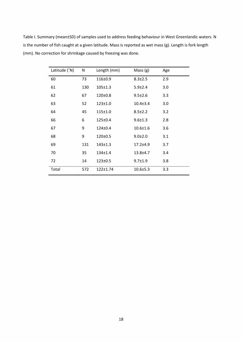
18
Table I. Summary (mean±SD) of samples used to address feeding behaviour in West Greenlandic waters. N
is the number of fish caught at a given latitude. Mass is reported as wet mass (g). Length is fork length
(mm). No correction for shrinkage caused by freezing was done.
Latitude (˚N) N Length (mm) Mass (g) Age
60 73 116±0.9 8.3±2.5 2.9
61 130 105±1.3 5.9±2.4 3.0
62 67 120±0.8 9.5±2.6 3.3
63 52 123±1.0 10.4±3.4 3.0
64 45 115±1.0 8.5±2.2 3.2
66 6 125±0.4 9.6±1.3 2.8
67 9 124±0.4 10.6±1.6 3.6
68 9 120±0.5 9.0±2.0 3.1
69 131 143±1.3 17.2±4.9 3.7
70 35 134±1.4 13.8±4.7 3.4
72 14 123±0.5 9.7±1.9 3.8
Total 572 122±1.74 10.6±5.3 3.3

19
Fig. 1
Composition of stomach content in capelin (N=572) from the Greenlandic west coast .The proportion made
up by the individual prey categories are reported based on wet mass (top) and by number (bottom).

20
Fig. 2
The relative contribution (of wet mass) of individual prey categories to the overall prey composition in
Greenlandic capelin at different latitudes along the Greenlandic west coast. The composition is reported for
both all sampled fish (top) and for fish within the same size range (115-130mm, bottom). See text for a
more detailed description of the individual prey categories. ■: Euphausiids, : Amphipods, ■: Copepods, □:
Other, : Unidentified.

21
Fig. 3
The left Y-axis and filled circles represent the relative amount of prey as a function of the latitude at which
the capelin were caught. The right Y-axis and open circles represent the mean stomach fullness (ranging
from 0-5) as a function of latitude. The line represents a fitted line to the relative amount of prey:
Y=41.7988x-0.3173x2-1364.759, R2=0.55, P=0.039. ●: relative prey wet mass, ○: stomach fullness.

22
Fig. 4
The proportion (% of wet mass) of three individual calanoid species to the overall composition of the
copepods (that were identified to species) in 115-130 mm Greenlandic capelin. Calanus finmarchicus and
Calanus glacialis are grouped together due to difficulties in correct identification due to digestion (●:
Calanus finarchicus/glacialis,: x: Calanus hyperboreus, ○: Metridia longa).

23
Fig. 5
The proportional (of wet mass) contribution of individual prey groups to the overall diet of capelin in
different size categories (mm, fork length). Data are from four areas along the Greenlandic west coast
(Qaqortoq, 59.5-61˚N, N=242; Nuuk, 63.5-65˚N, N=61; Disko, 69-70.5˚N, N=196; Uummannaq, 71.5-72.5˚N,
N=18). See text for more details on prey categories. ■: Euphausiids, : Amphipods, ■: Copepods, □: Other,
: Unidentified.
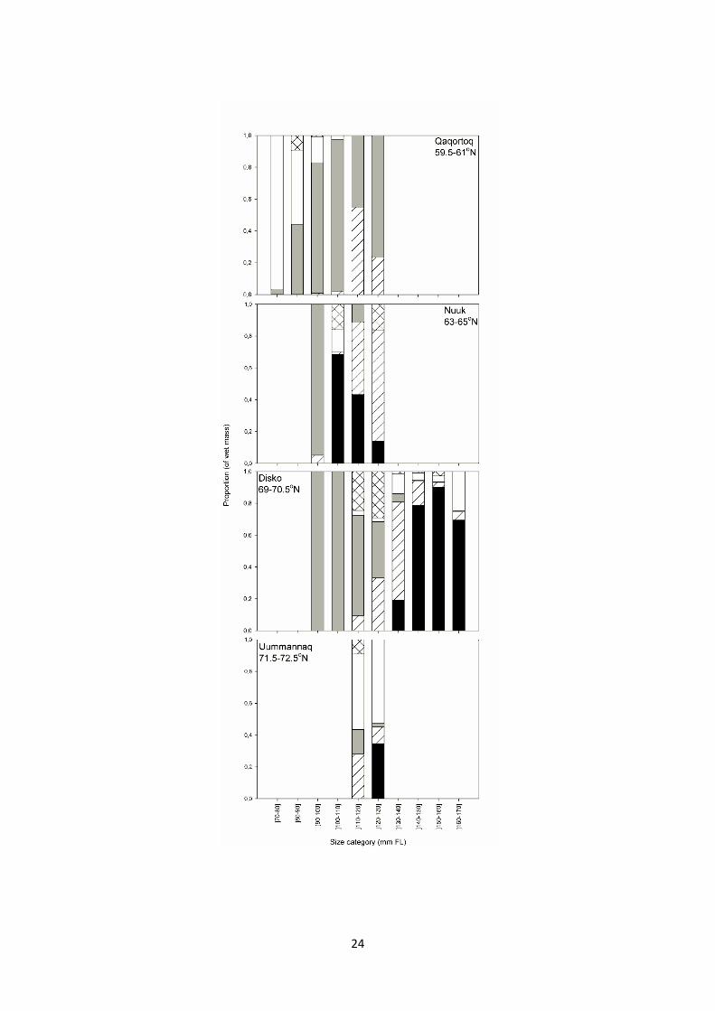
24

25
Fig. 6
Mean prey size (mm) of all prey from individual capelin as a function of capelin length (mm, fork length).
Data are from four areas along the Greenlandic west coast: ●: Qaqortoq (59.5-61˚N); ■: Nuuk (63.5-65˚N);
○: Disko (69-70.5˚N) and □: Uummannaq (71.5-72.5˚N).

26
Fig. 7
δ15N and δ13C values in capelin from the Greenlandic west coast. ●: Qaqortoq (59.5-61˚N); ■: Nuuk (63.5-
65˚N); ○: Disko (69-70.5˚N) and □: Uummannaq (71.5-72.5˚N); N=12 in all cases.

27
Fig. 8
δ15N and δ13C values in krill (Thysanoessa raschii) from the Greenlandic west coast. ●: Qaqortoq (59.5-61˚N,
N=4); ■: Nuuk (63.5-65˚N, N=3) and ○: Disko (69-70.5˚N, N=4). Each sample was taken from a homogenized
sample of 5-8 individuals and each point represents a mean value of these individuals. Data on Calanus
finmachicus, Calanus hyperboreus and Calanus glacialis are based on Møller (2007).

Paper II
Variation in size and growth of West Greenland capelin (Mallotus villosus) along
latitudinal gradients
R. Hedeholm, P. Grønkjær, A. Rosing-Asvid and S. Rysgaard
Published in ICES Journal of Marine Science

1
ICES Journal of Marine Science; doi:10.1093/icesjms/fsq024
Variation in size and growth of West Greenland capelin
(Mallotus villosus) along latitudinal gradients
R. Hedeholm1*, P. Grønkjær1, A. Rosing-Asvid2, and S. Rysgaard2
1Marine Ecology, Department of Biological Sciences, Aarhus University, Finlandsgade 14, 8200 Aarhus N, Denmark
2Greenland Climate Research Centre, c/o Greenland Institute of Natural Resources, PO Box 570, 3900 Nuuk, Greenland
*Corresponding Author: tel: +45 8942 4392; fax: +45 8942 4387; e-mail: [email protected].
Hedeholm, R., Grønkjær, P., Rosing-Asvid, A., and Rysgaard, S. 2010. Variation in size and growth of West Greenland capelin
(Mallotus villosus) along latitudinal gradients. – ICES Journal of Marine Science, doi:10.1093/icesjms/fsq024.
Received 21 September 2009; accepted 4 March 2010.
Capelin (Mallotus villosus) is the dominant pelagic species in the West Greenland ecosystem. Historical data
are re-examined and new data are presented on the size distribution and the growth pattern of capelin
along latitudinal gradients of temperature and other growth factors extending over a distance of 1300 km.
The average size of capelin increases with latitude. Fish 3 years old were 48 mm larger (54%) at the
secondmost northern station compared with the most southern one. Otolith analysis revealed a significant
effect of age as well as area on back-calculated growth. Hence, at all ages, fish grew faster in the north than
in the south. Average somatic growth across areas in the first and fourth years was 56 and 15 mm,
respectively. Temperature data suggest a 2˚C difference in temperature between areas, temperatures
being warmest in the north. Hence, the increase in temperature with latitude explains much of the
latitudinal growth gradient and suggests a growth difference in West Greenland capelin of 0.4–0.6 cm ˚C-1
year-1. However, the difference in growth and size distribution between northern and southernmost
stations, where temperatures are similar, suggests that other factors, such as differences in available prey
and diet composition, also contribute to the differences.
Keywords: capelin, Mallotus villosus, North Atlantic, temperature-regulated growth.

2
Introduction
Capelin (Mallotus villosus) are small osmerid fish with a circumpolar distribution. They are considered the
dominant pelagic species in Subarctic waters and important predators of zooplankton, as well as prey of
many species of fish (e.g. cod, haddock), birds (e.g. guillemot), and marine mammals (e.g. harp seal, minke
whale; Lawson et al., 1998; Vilhjálmsson, 2002). Some capelin stocks are commercially exploited, and
annual catches amounted to 746 534 t in 2005, with the main catches by Iceland and Norway. In some
years, Icelandic catches alone have been close to 2 million tonnes (Carscadden and Vilhjálmsson, 2002).
Capelin are found along the east and west coasts of Greenland from Kap Farvel in the south to Tassiilaq
(66˚N) and Upernavik (73˚N), respectively. The East Greenland capelin stock is often considered to be part
of the Icelandic stock (Vilhjálmsson, 2002), but the West Greenland stock is commercially unexploited and
little is known about capelin biology there (though see the review of Friis-Rødel and Kanneworff, 2002). It is
the latter stock that is the focus of the present study.
A latitudinal gradient in the size of West Greenland capelin was first reported by Hansen (1943), based
on historical data from 1906 on. These historical data, combined with new data, were analysed by
Kanneworff (1967), Sørensen (1985), and Kleist (1988). According to those studies, the maximum size of
capelin increases northwards along the coast. Kanneworff (1967) estimated the growth of capelin in the
Nuuk fjord system as well as at other West Greenland localities, although focus was on the fjord system.
However, he failed to find a major difference in the growth pattern between areas and did not address this
aspect further because of his small sample size. Sørensen (1985) suggested that the different maximum size
observed along the coast could be caused by differences in growth rates, although she did not present any
data or references. Hence, very little is known about the age specific growth pattern of Greenland capelin
and how this is expressed in the size distribution along the latitudinal gradient. The notion of a latitudinal
gradient has been based on historical data that often are associated with uncertainties (i.e. the length
measure applied, time and place of capture, age determination, etc.). Furthermore, in Greenland as well as
elsewhere, capelin size varies on an interannual basis (Gjøsæter, 1999; Carscadden and Frank, 2002), likely
obscuring patterns based on a compilation of historical data.
Temperature increase has a positive influence on growth in fish, where prey availability is non-limiting
and temperatures are below the optimum temperature for growth, which most often is the case
in temperate and boreal fish species (Gjøsæter and Loeng, 1987; Wootton, 1990; Brander, 1995; Garvey
and Marschall, 2003). The direct effect of temperature on capelin has been studied in the Barents Sea.
Gjøsæter and Loeng (1987) showed that annual temperature influences the capelin growth there, with
growth increasing by 0.3 cm ˚C-1.

3
In addition to temperature, food availability influences capelin growth in the Barents Sea (Gjøsæter et
al., 2002). The importance of feeding behaviour has been demonstrated in the Atlantic silverside (Menidia
menidia), another pelagic species, for which latitude-related growth differences were analysed by Conover
and Present (1990). Using laboratory-reared fish, they showed that fish caught farthest north had the
fastest growth rate, allowing them to compensate for the shorter growth season and to match the absolute
growth of fish at lower latitudes. Present and Conover (1992) demonstrated that this interpopulation
variation in growth rate was the result of increased consumption of food and a greater growth efficiency.
Therefore, in that case, the constraints on growth imposed by low temperatures were counterbalanced
by adaptations in feeding biology.
Temperature and length of the growing season differ considerably along the 1300-km north–south
distance evaluated here, so West Greenland capelin provide an opportunity to consider the possible effects
of climate change, which are thought to be most apparent in the Arctic region (Holland and Bitz, 2003). The
temperature differences observed along the latitudinal temperature gradient are comparable with the
changes expected in each of the areas investigated during the coming century (Levitus et al., 2000; Flato
and Boer, 2001), so the present data provide insights into possible future changes in growth and size of
Greenland capelin.
Here, we re-examine the historical data on capelin in Greenland to demonstrate a historical difference in
the size distribution in different areas. We use contemporary data for which otoliths are available to
elucidate whether these differences result from differences in growth rate along the observed latitudinal
gradients of temperature and other factors.
Material and methods
Study site and 2007 sampling
All 2007 samples were collected on the west coast of Greenland. Four areas spanning 1300 km were
selected for further study: Qaqortoq (60–61˚N), Nuuk (64.00–64.75˚N), Disko (68.50–69.50˚N), and
Uummannaq (70.30–71.30˚N; Figure 1). The latitudinal borders were selected according to hydrographic
and topographic features and their comparability with the historical data. Within each area, capelin were
collected during beachspawning events using handnets. In all, 461 fish were sampled with 88, 219, 79, and
75 individuals, respectively, being collected from south to north at the different locations. Samples were
collected from as many spawning sites within each area as possible between 11 May and 19 July, with no
relation between latitude and sampling time. All samples were deep-frozen and brought to the laboratory,
then upon thawing, all fish were measured to the nearest millimetre below (fork length), sexed, dried, and

4
weighed to the nearest 0.1 g. No correction for length changes caused by freezing was applied, which might
have introduced an error of up to 3% (Sørensen, 1985). When comparisons with historical samples were
made, fork length was converted to standard length using the relationship for Greenland capelin
documented by Kanneworff (1967), i.e. standard length = 0.92 × fork length + 0.042. The relationship was
confirmed using a random subsample of fish sampled in 2007 across all areas.
Latitudinal gradients in capelin size
The historical samples were from 1908 to 2005, although several years are not represented. Most samples
(>90%) were from spawning events taken using dipnets and hand-seines, though pelagic trawls were used
at greater depth and outside the spawning season on a few occasions. A few samples were caught in
poundnets and gillnets aimed at cod (Gadus morhua). Only fish caught in the areas sampled in 2007 were
used. All sampled fish were measured, weighed, and in some cases aged and sexed. All measurements
before 1967 were made to the nearest 0.5 cm below. To allow comparisons with new material, 0.25 cm
(0.5 unit) was added to these measurements. From 1967 to 2005, all measurements were to the nearest
millimetre below. Samples that differed greatly from what should be expected (e.g. mean length or weight,
time of sampling, place of sampling, or duplicates) were investigated and excluded from further analysis
if errors were found. Moreover, as the sexes differ in size and males dominated the 2007 sample, all
females and unsexed individuals were excluded. These criteria reduced the initial historical sample size
from 45 810 to 13 990 capelin, but the reduction was justified by a large increase in data quality (Table 1).
The size distribution of the historical data was plotted for the four areas to determine whether any
latitudinal differences in size have been evident historically.
All fish caught in 2007 were assigned to length intervals of 2 mm, and the length frequency distributions
were calculated for the four areas. To ensure that any pattern found was not due to different age groups
being more or less represented in different areas, the average length of all 3-year-old males from 2007 was
plotted as a function of the latitude at which they were caught. Fish 3 years old were used because that
was the age group that dominated samples (n = 176) when all areas were considered. The other age groups
produced patterns identical to those shown by 3-year olds (data not shown). When fish were caught at
several latitudes within each of the four areas, the average latitude and length was used, and no weighting
in terms of sample size was applied.
Otolith-based growth analysis
Only males were used in growth studies because of the scarcity of females (n = 45) and the belief that some
females survive spawning, which might produce otolith structures that would make the interpretation and
5
subsequent analysis difficult (Sørensen, 1985; Kleist, 1988; Friis-Rødel and Kanneworff, 2002). The saggital
otoliths were removed, rinsed in water, and dried. As growth increments in capelin are prominent, it was
sufficient to submerge the otoliths in alcohol and place them on a black background. Age determinations
were carried out independently by two readers. When discrepancies were found (<10% overall), the
otoliths were re-analysed and discarded if the age could not be determined with certainty. There was no
age bias in the discarded otoliths. Using a stereoscope and an Olympus DP50 camera, all otoliths were
photographed at different magnification (×16–40) under reflected light. The pictures with the clearest
growth increments were selected for further analysis. Using “Image-J” image analysis software (Rasband,
1997–2007), a line was drawn from the rostrum through the otolith centre (Line 1 in Figure 2). A line was
also drawn from the centre of the otolith to the edge of the otolith, along which the growth increments
(mm) were determined (Line 2 in Figure 2). The latter line was drawn so that it was perpendicular to the
growth rings. The total otolith radius was defined as the sum of all measured growth increments along that
line. All growth increments were measured to the end of the translucent zone. The process was repeated
twice for each otolith, and if the measurements differed by >10%, they were discarded; if not, the mean of
the two measurements was used in further analysis. Owing to the small sample size (n = 19), growth
between 4 and 5 years of age was not used in the analysis. To compare somatic growth between
areas independent of differences in the relationship between otolith size and fish length between areas,
length-at-age was backcalculated using the biological intercept method (Campana, 1990):
La = Lc + (Oa − Oc) × (Lc − Li) × (Oc − Oi)-1,
where La is the length at a given age, Lc the length at capture, Oa the otolith radius at a given age, Oc the
total otolith radius at capture, Li the length of fish at the biological intercept, and Oi the otolith radius at
biological intercept. The biological intercept was set at a fish length of 35 mm and an otolith size of 0.08
mm (Gjøsæter, 1999). Growth was then calculated by subtracting length-at-aget from length-at-aget+1, and
plotted for each age and area.
To validate the timing of the first growth increment, sagittae from young of the year (YOY) caught on 12
September in the Nuuk area were analysed (n = 6). Because of the late sampling date, it was assumed that
the growth season was complete but that the translucent (winter) increment had not yet formed. Hence,
the test was to determine whether the radius of YOY otoliths was similar to the radius of the first opaque
(summer) increment in adult fish caught in the Nuuk area. To ensure that the innermost growth increment
was measured correctly, a random sample of 10 saggital pairs was selected from all areas. One otolith from
each pair was polished on grain size 800 sandpaper until the innermost increment was at its clearest, then
the growth increment was re-measured and compared with the measurement of the unpolished otolith.

6
The first-growth increment sizes of the re-measured polished otoliths were similar to those of the
unpolished ones (Student’s t-test, t10 = 0.11, p = 0.917), so polishing was not deemed necessary.
Owing to the time of sampling, adult fish were assumed to have experienced almost a full growth
season, and the marginal growth increment was considered to constitute a full growth season. To validate
this assumption, the marginal growth increment of the most abundant year class within an area was
compared with the growth increment in older fish in their corresponding growth year within the same area.
For instance, at Qaqortoq, the marginal growth increment in 3-year-old capelin was compared with the
third-year growth in 4- and 5-year-old fish. This was done for all areas. Had the fish not completed the
growth season, older fish would have had wider increments than younger fish.
Temperature and salinity
To evaluate temperature differences along the latitudinal gradient, all available temperature data for West
Greenland (60–73˚N 44–57˚W) were extracted from the ICES database (www.ices.dk; n = 114 072). As all
literature indicates that Greenland capelin are restricted to fjords and near-coastal waters (see review by
Friis-Rødel and Kanneworff, 2002), all measurements taken at locations where the bottom depth exceeded
500 m were excluded. This ensured that no data west of the shelf break were used. Moreover, all
measurements from 0 to 20 m were discarded because these may be influenced by episodic disturbances
such as freshwater inflow. As capelin in the feeding period primarily reside in the upper water layers, and
more so at younger life stages (Gjøsæter, 1998), measurements from 20 to 50 m were used. Data deeper
than 50 m could well have been included because adult capelin make diurnal vertical migrations (Sørensen,
1985; Gjøsæter, 1998), but the same general pattern in latitudinal temperature trends was observed when
data from 10 to 100 m were used. However, those data showed more variability because progressively
fewer years were available for analysis (the data are therefore not shown).
Temperature data were averaged for all stations. As capelin growth is most rapid in summer, data for
July (n = 1 137), August (n = 478), and September (n = 282) were considered separately. The plots were
constructed by assigning each temperature to the nearest latitudinal degree, then taking the unweighted
average of all years at all latitudes, so avoiding overrepresentation of an unusually warm or cold year. In all,
data from 78 years were used, spanning almost a century (1908–2007). Usually, salinity was determined
along with temperature measurements (n = 17 489), and was also extracted from the ICES database, and
used to determine possible differences in the origin of water masses at the different locations. To avoid
overrepresentation of certain (cold or warm) months, only data from August are presented here (n = 1
362).

7
Statistical analysis
All analyses were carried out using SPSS (Statistical Package of Social Sciences). Standard parametric tests
were preceded by tests for assumptions. When these were violated, the data were either transformed or
non-parametric statistics were applied.
Results
Latitudinal size gradient
Length frequencies for historical data and for 2007 samples are shown in Figure 3. The historical data show
that capelin are largest at Disko, with an average male size of 155 + 14.3 mm (s.d.). Average size then
declines northwards to Uummannaq (144 + 7.3 mm) and southwards to Nuuk (122 + 14.6 mm). At the
southernmost point of sampling, Qaqortoq, average size increased to 139 + 12.9 mm. Hence, although
capelin appeared to be bigger in the northern area, there was no obvious latitudinal gradient, because fish
from Qaqortoq were as big as capelin caught farther north. Focusing instead on the 2007 data, the size
distribution at Qaqortoq shifted towards smaller sizes than the historical data, an effect that was most
evident in the decrease in average size, to 88 mm in the 2007 samples. Therefore, the average sizes
from south to north in the 2007 samples were 88 + 11.5, 120 + 10.3, 146 + 20.5, and 137 + 8.8 mm,
respectively. The lengths of 3-year-old males in 2007 (n = 176) also revealed that mean length was related
to latitude (one-way ANOVA, F3,172 = 398.040, p < 0.0005), with all areas except the two northern areas
(Tukey’s post hoc test, p = 0.054) being significantly different (Tukey’s post hoc test, p < 0.0005; Figure 4).
Growth analysis
There was a clear positive relationship between otolith radius (Figure 2) and length (Figure 5), justifying the
assumption of a relationship between otolith growth and somatic growth (linear regression, F1,183 = 375.79,
r2 = 0.67, p < 0.0005). The determination and the interpretation of the first and marginal growth increments
were also supported by the analysis. Comparisons of the marginal growth increment of the most abundant
age group with the corresponding growth increment in older fish showed that the older fish had similar
increments. Only fish from Qaqortoq had marginal increments significantly different from the
corresponding increment of older fish (one-way ANOVA, F1,29 = 28.32, p < 0.01; Table 2), indicating that the
growth season was over at the time of sampling. The first growth increment in YOY (i.e. total otolith
radius) from Nuuk had an average size of 0.103 mm, significantly smaller than the radius of the first opaque
increment in adult fish caught in the same area (0.134 mm; Student’s t-test, t44 = 2.83, p = 0.007). However,
the absolute difference in radius (0.031 mm) is small enough to justify the assumption that the first growth
increment was determined correctly.

8
Growth patterns for males caught in 2007 in the four areas are presented in Figure 6. An analysis of
covariance (ANCOVA) was performed to determine the effect of area and age on logtransformed growth
increments (linear regression, F1,79 – 158 ≥ 164.005, p < 0.0005). The full factorial model showed an effect of
area (ANCOVA, F3,540 = 4.753, p = 0.003) and age (ANCOVA, F1,540 = 1082.664, p < 0.0005), but also a
significant interaction between area and age (ANCOVA, F3,540 = 8.557, p < 0.0005), demonstrating that
differences in growth could not be based solely on area. However, this significant interaction was primarily
caused by irregular growth in the northernmost area (Uummannaq), as seen in Figure 6. In the 0+ period,
growth was the second lowest of the four areas (55 mm), but highest in the 2+ period (42.7 mm). Another
anomaly was the increase in growth from 1+ to 2+ (38.0 and 42.7 mm, respectively), which was not seen in
the other areas. However, removing Uummannaq from the analysis did not render the interaction
insignificant (p = 0.003). Overall, it appears that capelin of all ages grow faster at Disko than at Nuuk and
Qaqortoq, whereas capelin at Nuuk grow faster than those from Qaqortoq, and that somatic growth
declines significantly as the fish age in all areas. However, the growth pattern can be seen as reflecting
three separate life stages and not necessarily a steady growth decline. Growth in the first year is fast, but
more moderate in the second and third years. In the fourth year, the capelin approach their spawning
age, and growth is at its minimum.
Temperature and salinity
According to the ICES temperature database, average temperatures increase from south to north (Figure
7). Considering all months, the temperature was close to 1˚C at 60˚N, increasing to 2˚C at 68˚N, then
declining towards the north. The same pattern was evident for the three selected months, but with greater
latitudinal differences. Hence, there was a 2˚C difference between 60˚N and 68˚N in July, August, and
September, with individual temperatures varying by 18C between months. The drop in temperature
of ~1˚C from the Disko area to Uummannaq was also apparent in all 3 months.
Salinity also changed with latitude, increasing from 32.3 in the south to 33.4 in the Disko area, and
dropping to 33 in Uummannaq (Figure 8). Salinity in the Nuuk area does not follow the overall trend,
displaying values well below those of adjacent latitudes (32.5), probably because of the outflow of
freshwater from the Nuuk fjord.
Discussion
Growth pattern
Both historical and new data show a latitudinal variation in the size of male West Greenland capelin. In the
contemporary data, average size increases with latitude except in the area farthest north (Uummannaq),

9
where it declines slightly. This size gradient is not a result of altering age distribution along the coast,
because the pattern is the same in the average size of 3-year-old males (Figure 4), and the growth analysis
showed that the gradient was expressed at all ages (Figure 6). Uummannaq differs from the other areas in
that growth rates there do not decline consistently with age, being unexpectedly high in the period 2+.
In the historical data, the pattern is the same, except at Qaqortoq where the size distribution is skewed
towards larger sizes than in the 2007 data. There could be several reasons for this. As a large proportion
(>80%) of the samples were caught offshore, the distribution could be skewed by containing capelin that
might have migrated or drifted from the east coast around the southern tip of Greenland, creating a
sampling bias (Wileman et al., 1996). This would skew the distribution, because capelin in East Greenland
are larger (Hansen, 1943; Vilhjálmsson, 1994). However, this does not appear to be the case when
comparing historical trawl catches with other sampling gear, though insufficiency of information on
catching methods renders such conclusions tentative. Additionally, the spawning stock could historically
have been dominated by larger East Greenland capelin, whereas the present-day spawning stock is
mainly small fish. As otoliths are available for the 2007 samples, however, the present-day gradient is
deemed correctly determined, and the reason for the discrepancy with historical data is unknown.
Therefore, we believe that the growth gradient demonstrated using the 2007 samples represents the
current situation, although this needs to be supported by more study, to allow for additional comparison
with the historical information.
Only one peak in size distribution was observed always, despite there likely being multiple cohorts in the
samples, because sampling was concentrated in the spawning season, which homogenizes the distribution
for two reasons. First, the spawning population consists primarily of a single cohort (Bailey et al.,
1977; Vilhjálmsson, 1994) and, second, it is mainly the larger fish of a cohort that spawn (Friis-Rødel and
Kanneworff, 2002), which further reduces the size variation.
Our study focused solely on male growth. Female growth of Greenland capelin was researched by
Kanneworff (1967), who showed that females grew slower than males and achieved a smaller maximum
size. However, males and females most likely differ in life strategy, being semelparous and iteroparous,
respectively (Huse, 1998; Carscadden et al., 2001; Friis-Rødel and Kanneworff, 2002). As a result, female
growth increments may be erratic in repeat spawners, which makes growth interpretation difficult and
does not allow comparison between first-time and repeat spawners (Kleist, 1988).
To validate otolith interpretation, three issues were addressed: (i) whether the fish had completed a full
growth season as assumed, (ii) whether the first growth increment was measured correctly, and (iii)
whether the timing of laying down of the first increment was correct. Assumptions (i) and (ii) were met, but

10
YOY from the Nuuk area had a smaller first growth increment than adult fish from the same area (0.103 and
0.134 mm, respectively). We feel confident that the small difference is not attributable to the first growth
increment being wrongly determined, but rather to the growth season in YOY being incomplete, with the
growth period extending beyond mid-September for that age group. In addition, size-selective mortality in
later life with smaller fish of a cohort having a greater mortality rate could cause a wider first increment in
surviving fish than in YOY. These growth patterns may arise from either inherent genetic differences or
environmental effects. Such effects are likely to be linked to temperature and prey availability.
Greenland capelin display some degree of genetic differentiation (Sørensen and Simonsen, 1988).
Genetic differences along latitudinal gradients influence growth patterns in Atlantic silverside (Conover and
Present, 1990; Present and Conover, 1992) and could well explain a proportion of the growth variation
demonstrated here, especially given that the selective forces (low winter temperature and a short growing
season) proposed to have generated the genetically based growth differences in the silverside are the same
in Greenland waters.
However, as no thorough and recent genetic studies on Greenland capelin exist and no controlled
experimental work addressing the genetic influence on phenotypic variation has been performed, a genetic
effect cannot yet be quantified. Hence, latitudinal growth variation is discussed based on available
environmental data, although future exploration of a possible genetic component is encouraged. A further
advantage at higher latitudes that should also be considered by future work is the increase in the daily
feeding period for active visual predators associated with an increase in daylight hours, as demonstrated
for juvenile cod by Suthers and Sundby (1996).
Temperature effect
The average growth of West Greenland capelin shown here is similar to that of other capelin populations in
terms of absolute growth as well as the decline in growth with age (Templeman, 1948; Vilhjálmsson, 1994;
Gjøsæter et al., 2002). Latitudinal growth differences have been shown in Barents Sea capelin by Gjøsæter
and Loeng (1987), who calculated growth from six areas in the period 1974–1985. They found a 15.5 mm
reduction in growth with increasing latitude (71–77˚N) in the last growth season of 2-year-old fish, similar
to the 12.9 mm we found over a greater distance (61–69˚N). However, the growth pattern was reversed,
with growth being least in the north in their study. The growth difference is most likely caused by a large
temperature difference between the subareas in the Barents Sea, because Gjøsæter and Loeng (1987)
demonstrated a growth increase of 0.3 cm ˚C-1 year-1 in both 2- and 3-year-old fish, using sea surface (10–
200 m) temperatures. Obviously, the relationship between growth and temperature is not necessarily
linear and may differ between ages, but assuming that the same relationship applies to West Greenland

11
capelin and calculating the growth difference in 2- and 3-year-old fish for comparison, the expected
experienced temperature difference between Qaqortoq (60˚N) and Disko (69˚N) should be between 2.8˚C
for 2-year olds and 4.3˚C for 3-year olds. The temperature data analysed (Figure 7) showed an increase
from Qaqortoq to Disko and a decline at Uummannaq, a trend similar to that of fish growth (Figures 4 and
6), growth being lowest at Qaqortoq, highest at Disko, and dropping slightly at Uummannaq. The large
temperature drop at Uummannaq could be expected to cause a more pronounced growth decrease than
observed, however. As the temperature drop is over a relatively short distance, the capelin may escape
the unfavourable growth environment through annual migrations, as elsewhere (Vilhjálmsson, 2002).
However, capelin migration patterns have not been investigated in West Greenland waters.
The inverse relationship between temperature and latitude along the west coast of Greenland is caused
by mixing of the dominant currents in the area. East of Greenland, cold saline Polar Water (PW; Figure 1)
that lies inshore along the Greenland coast meets offshore warmer, highly saline Irminger Sea Water
(IW; Figure 1). The two currents progressively mix as they flow clockwise around the coast of Greenland,
causing gradual warming of the inshore surface waters towards the north (see review by Buch, 2000;
Ribergaard, 2007). This was also evident from the salinity measurements made simultaneously with the
temperature recordings (Figure 8), which show an increase in salinity with latitude in accordance with the
gradual mixing shorewards of the more saline, warmer Irminger Water. In comparison, the salinity of pure
Irminger Water and Polar Water is ca. 35 and 32, respectively (Ribergaard et al., 2008), confirming the
presence of Polar Water in the surface layers in the south. Salinity in the Nuuk area did not follow the
overall trend (Figure 8). This may be due to many (ca. 20%) of the measurements being made at the
opening of the fjord, where there is a high degree of mixing and a substantial input of freshwater run-off
from glaciers in summer (Mikkelsen et al., 2008).
Additional data on Greenland west coast temperature are found in Ribergaard (2007), who made CTD
measurements along the Greenland west coast in March, May, and July 2006. He showed that temperature
near the coast was similar across latitudes. However, there was a tendency towards the upper layers (<200
m) being 1–28C warmer at higher latitudes and for the temperature to drop again north of Disko.
Ribergaard (2007) also measured temperatures in three fjords along the coast and in Disko Bay, yielding the
same result, i.e. a small temperature increase from south to north. Munk et al. (2003) presented data from
a northern subset of the area covered by Ribergaard (2007), measured in late June and early July 1996, and
documented small differences between areas of 1–2˚C, but no clear latitudinal gradient. Finally, a capelin
trial fishery in September and October 2005 made CTD measurements from 59 to 73˚N

12
(Bergstrøm and Vilhjálmsson, 2006). The measurements were made east and west of the banks. From 0 to
20 m, the temperature was at least 2–3˚C higher in the north, but deeper than 50 m, the pattern was
reversed.
Therefore, the available temperature data are not conclusive, but the ICES data used here suggest a
latitudinal temperature gradient in the upper water layers, with temperatures ca. 2˚C higher in the capelin
growth season at Disko than at Qaqortoq. This suggests that the effect of temperature on growth is greater
in West Greenland capelin than in Barents Sea capelin (0.4–0.6 and 0.3 cm ˚C-1 year-1, respectively).
The decline in average size and the unique age-specific growth pattern in the Uummannaq area may be a
result of pronounced year-to-year temperature variation in this area. Capelin live close to their northern
boundary at Uummannaq, where the yearly average temperature is ~0.8˚C, and in warm years, they have
been found farther north and in colder years farther south (Hansen and Hermann, 1953; Friis-Rødel and
Kanneworff, 2002). The growth of capelin there may therefore be more variable, and the increased growth
seen in 2+ fish in Uummannaq does coincide with the majority of the sampled fish (50%) experiencing
a warm 2006 in the 2+ growth season (Ribergaard, 2007).
Prey effects
Although the temperature regime appears to be a likely explanation for the latitudinal size variation, the
fact that Qaqortoq and Uummannaq capelin show very different growth rates despite similar average
annual temperatures, whereas Uummannaq and Disko capelin show similar growth despite different
temperatures suggests that other factors may be playing a role too.
Capelin growth rates have been correlated with zooplankton abundance (Gjøsæter et al., 2002), and
because we analysed a large latitudinal gradient, prey availability and quality may have differed between
areas. Studies on zooplankton abundance along the Greenland west coast suggest a similar abundance of
prey species between areas (Pedersen and Smidt, 2000; Levinsen and Nielsen, 2002; Jensen and Rasch,
2008). However, there appears to be a shift in dominant species. Towards the north, the copepod
community is increasingly dominated by the large Calanus hyperboreus, replacing the smaller Calanus
finmarchicus. This is also evident in the results of a recent unpublished feeding study on Greenland capelin,
in which the former (larger) species gradually replaced the latter (smaller) one in capelin stomach contents
towards the north. This may give the northern species an increased energy intake, especially in the
youngest stages where copepods dominate the diet (O’Driscoll et al., 2001). In larger capelin, krill became
increasingly more important as prey with latitude. As krill are larger and with similarly high energy content
(Falk-Petersen et al., 2000), this may infer some feeding advantage for large capelin in the north. Hence,
latitudinal feeding differences at all life stages may contribute to maintaining the growth gradient in West

13
Greenland capelin seen in other waters (Gjøsæter et al., 2002). Moreover, a shift in energy consumption of
capelin, and therefore in its own growth potential and energy content, can affect higher trophic levels, as
seen in sprat (Sprattus sprattus) in the Baltic (Cardinale et al., 2002; MacKenzie and Köster, 2004;
Österblom et al., 2006) and in North Sea herring (Clupea harengus; Alheit et al., 2005).
In addition to prey abundance, capelin abundance may also affect feeding possibilities. Hence, if capelin
abundance is low in the north, the food intake per capita may be higher than elsewhere, although evidence
of density-dependent processes is equivocal (Millner and Whiting, 1996; Melvin and Stephenson, 2007).
Abundance estimates of Greenland capelin are scarce. In 2005, an attempt was made to quantify capelin
abundance along the Greenland west coast (Bergstrøm and Vilhjálmsson, 2006), and it suggested that
density was highest in the Disko area (233.8 t nautical mile-1) and the Nuuk fjord system (170.2 t nautical
mile-1), and lowest in the south (42.0 t nautical mile-1). Based on these findings, capelin density should, if
anything, limit growth in the northern part of the study area, and density dependence is not likely to play a
role in the growth regulation we have documented.
Conclusions
In summary, growth differences in West Greenland capelin are related to the 2˚C difference between the
areas studied. Hence, predictions of increased future temperatures along Greenland (Stendel et al., 2008)
will most likely affect the growth of Greenland capelin, and consequently the entire West Greenland
ecosystem. Such changes are attributable to the direct effect of temperature on growth and metabolism,
but the effect is likely to be modified by concurrent changes in prey availability and energy changes in prey
composition. Therefore, the effects might be many and non-linear, making an overall response of both
capelin and the ecosystem likely, but not easily predictable.
Acknowledgements
We thank the staff at the Greenland Institute of Natural Resources for help with sampling and processing of
the temperature data, as well as in interpreting the otoliths. Holger Hovgård, Kaj Sünksen, Arne Geisler, and
Aili Lage Labansen in particular provided appreciated assistance. Additionally we thank two anonymous
reviewers for helpful comments on an earlier version of the manuscript.

14
References
Alheit, J., Möllmann, C., Dutz, J., Kornilovs, G., Loewe, P., Mohrholz, V., and Wasmund, N. 2005.
Synchronous ecological regime shifts in the central Baltic and the North Sea in the late 1980s. ICES
Journal of Marine Science, 62: 1205–1215.
Bailey, R. F. J., Able, K. W., and Leggett, W. C. 1977. The seasonal and vertical distribution and growth of
juvenile and adult capelin (Mallotus villosus) in the St Lawrence Estuary and western Gulf of St Lawrence.
Journal of the Fisheries Research Board of Canada, 34: 2030–040.
Bergstrøm, B., and Vilhjálmsson, H. 2006. Cruise report and preliminary results of the acoustic/pelagic trawl
survey offWest Greenland for capelin and polar cod 2006. Greenland Institute of Natural Resources.
60pp.
Brander, K. M. 1995. The effect of temperature on growth of Atlantic cod (Gadus morhua L.). ICES Journal
of Marine Science, 52: 1–10.
Buch, E. 2000. A monograph on the physical environment of Greenland waters. Greenland Fisheries
Research Institute Report. 405 pp.
Campana, S. E. 1990. Analysis of otolith microstructure data. In Otolith Microstructure Examination and
Analysis, pp. 73–110. Ed. by D. K. Stevenson, and S. E. Campana. Canadian Special Publication of Fisheries
and Aquatic Sciences, 117.
Cardinale, M., Casini, M., and Arrhenius, F. 2002. The influence of biotic and abiotic factors on the growth
of sprat (Sprattus sprattus) in the Baltic Sea. Aquatic Living Resources, 15: 273–281.
Carscadden, J. E., and Frank, K. T. 2002. Temporal variability in the condition factors of Newfoundland
capelin (Mallotus villosus) during the past two decades. ICES Journal of Marine Science, 59: 950–958.
Carscadden, J. E., Frank, K. T., and Leggett, W. C. 2001. Ecosystem changes and the effects on capelin
(Mallotus villosus), a major forage species. Canadian Journal of Fisheries and Aquatic Sciences, 58: 73–85.
Carscadden, J. E., and Vilhjálmsson, H. 2002. Capelin – what are they good for? Introduction. ICES Journal of
Marine Science, 59: 863–869.
Conover,D.O., and Present, T. M. C. 1990.Countergradient variation in growth-rate—compensation for
length of the growing-season among Atlantic silversides from different latitudes. Oecologia, 83: 316–324.
Falk-Petersen, S., Hagen, W., Kattner, G., Clarke, A., and Sargent, J. 2000. Lipids, trophic relationships, and
biodiversity in Arctic and Antarctic krill. Canadian Journal of Fisheries and Aquatic Sciences, 57(Suppl. 3):
178–191.
Flato, G. M., and Boer, G. J. 2001. Warming asymmetry in climate change simulations. Geophysical
Research Letters, 28: 195–198.

15
Friis-Rødel, E., and Kanneworff, P. 2002. A review of capelin (Mallotus villosus) in Greenland waters. ICES
Journal of Marine Science, 59: 890–896.
Garvey, J. E., and Marschall, E. A. 2003. Understanding latitudinal trends in fish body size through models of
optimal seasonal energy allocation. Canadian Journal of Fisheries and Aquatic Sciences, 60: 938–948.
Gjøsæter, H. 1998. The population biology and exploitation of capelin (Mallotus villosus) in the Barents Sea.
Sarsia, 83: 453–496.
Gjøsæter, H. 1999. Studies on the Barents Sea capelin (Mallotus villosus Müller), with emphasis on growth.
Thesis, University of Bergen. 160 pp.
Gjøsæter, H., Dalpadado, P., and Hassel, A. 2002. Growth of Barents Sea capelin (Mallotus villosus) in
relation to zooplankton abundance. ICES Journal of Marine Science, 59: 959–967.
Gjøsæter, H., and Loeng, H. 1987. Growth of the Barents Sea capelin, Mallotus villosus, in relation to
climate. Environmental Biology of Fishes, 20: 293–300.
Hansen, P. M. 1943. Capelin (Mallotus villosus). Annales Biologique du Conseil Permanent International
pour l’Exploration de la Mer, 1: 121–124.
Hansen, P. M., and Hermann, F. 1953. Fisken og havet ved Grønland [The Fish and Ocean at Greenland].
Danmarks Fiskeri- og Havundersøgelser, Copenhagen. 128 pp.
Holland, M. M., and Bitz, C. M. 2003. Polar amplification of climate change in coupled models. Climate
Dynamics, 21: 221–232.
Huse, G. 1998. Sex-specific life history strategies in capelin (Mallotus villosus)? Canadian Journal of Fisheries
and Aquatic Sciences, 55: 631–638.
Jensen, L. M., and Rasch, M. (Eds). 2008. Nuuk Ecological Research Operations, 1st Annual Report 2007.
Nuuk Ecological Research Operations. Danish Polar Centre, Copenhagen. 112 pp.
Kanneworff, P. 1967. Mallotus villosus(O. F.Müller). Biologi og dynamik i grønlandske farvande. [Mallotus
villosus (O. F. Mu¨ller). Biology and dynamics in Greenland waters]. Thesis, Grønlands
Fiskeriundersøgelser, Copenhagen. 103 pp.
Kleist, J. 1988. Ammassat (Mallotus villosus) i Sydvestgrønland. [Capelin (Mallotus villosus) in Southwest
Greenland]. Thesis,Grønlands Fiskeriundersøgelser, Copenhagen. 67 pp.
Lawson, J. W., Anderson, J. T., Dalley, E. L., and Stenson, G. B. 1998. Selective foraging by harp seals Phoca
groenlandica in nearshore and offshore waters of Newfoundland, 1993 and 1994. Marine Ecology
Progress Series, 163: 1–10.
Levinsen, H., and Nielsen, T. G. 2002. The trophic role of marine pelagic ciliates and heterotrophic
dinoflagellates in Arctic and temperate coastal ecosystems: a cross-latitude comparison. Limnology
and Oceanography, 47: 427–439.

16
Levitus, S., Antonov, J. I., Boyer, T. P., and Stephens, C. 2000. Warming of the world ocean. Science, 287:
2225–2229.
Mackenzie, B. R., and Köster, F.W. 2004. Fish production and climate: sprat in the Baltic Sea. Ecology, 85:
784–794.
Melvin, G. D., and Stephenson, R. L. 2007. The dynamics of a recovering fish stock: Georges Bank herring.
ICES Journal of Marine Science, 64: 69–82.
Mikkelsen, D. M., Rysgaard, S., Mortensen, J., Retzel, A., Nygaard, R., Juul-Pedersen, T., Sejr, M., et al. 2008.
The MarineBasic Programme 2007. In Nuuk Ecological Research Operations, 1st Annual Report. Ed. by L.
M. Jensen, and M. Rasch. Danish Polar Centre, Copenhagen.
Millner, R. S., and Whiting, C. L. 1996. Long-term changes in growth and population abundance of sole in
the North Sea from 1940 to the present. ICES Journal of Marine Science, 53: 1185–1195.
Munk, P., Hansen, B. W., Nielsen, T. G., and Thomsen, H. A. 2003. Changes in plankton and fish larvae
communities across hydrographic fronts off West Greenland. Journal of Plankton Research, 25: 815–830.
O’Driscoll, R. L., Parsons, M. J. D., and Rose, G. A. 2001. Feeding of capelin (Mallotus villosus) in
Newfoundland waters. Sarsia, 86: 165–176.
Österblom, H., Casini, M., Olsson, O., and Bignert, A. 2006. Fish, seabirds and trophic cascades in the Baltic
Sea. Marine Ecology Progress Series, 323: 233–238.
Pedersen, S. A., and Smidt, E. L. B. 2000. Zooplankton distribution and abundance in West Greenland
waters, 1950–1984. Journal of Northwest Atlantic Fisheries Science, 26: 45–102.
Present, T. M. C., and Conover, D. O. 1992. Physiological basis of latitudinal growth differences in Menidia
menidia—variation in consumption or efficiency. Functional Ecology, 6: 23–31.
Rasband, W. S. 1997–2007. ImageJ. National Institutes of Health, Bethesda, MD, http://rsb.info.nih.gov/ij/.
Ribergaard, M. H. 2007. Oceanographic investigations off West Greenland 2006. Danish Meteorological
Institute Centre for Ocean and Ice. 49 pp.
Ribergaard, M. H., Olsen, S. M., and Mortensen, J. 2008. Oceanographic investigations off West Greenland
2007. Danish Meteorological Institute Centre for Ocean and Ice. 48 pp.
Sørensen, E. F. 1985. Ammassat ved Vestgrønland [Capelin at West Greenland]. Fiskeri- og
Miljøundersøgelser i Grønland. 82 pp.
Sørensen, E. F., and Simonsen, V. 1988. Genetic differentiation among populations of capelin Mallotus
villosus from the west coast of Greenland. Journal of Applied Ichthyology, 4: 23–28.
Stendel, M., Christensen, J. H., and Petersen, D. 2008. Arctic climate and climate change with a focus on
Greenland. Advances in Ecological Research, 40: 13–43.

17
Suthers, I. M., and Sundby, S. 1996. Role of the midnight sun: comparative growth of pelagic juvenile cod
(Gadus morhua) from the Arcto-Norwegian and a Nova Scotian stock. ICES Journal of Marine Science, 53:
827–836.
Templeman, W. 1948. The life history of the capelin (Mallotus villosus O. F. Mu¨ller) in Newfoundland
waters. Research Bulletin of the Newfoundland Government Laboratory, 17. 151 pp.
Vilhjálmsson, H. 1994. The Icelandic capelin stock. Capelin (Mallotus villosus) in the Iceland–East
Greenland–Jan Mayen area. Rit Fiskideildar, 13. 281 pp.
Vilhjálmsson, H. 2002. Capelin (Mallotus villosus) in the Iceland–East Greenland–Jan Mayen ecosystem.
ICES Journal of Marine Science, 59: 870–883.
Wileman, D. A., Ferro, R. S. T., Fonteyne, R., and Millar, R. B. (Eds). 1996. Manual of methods of measuring
the selectivity of towed fishing gears. ICES Cooperative Research Report, 215. 126 pp.
Wootton, R. J. 1990. Ecology of Teleost Fishes, 2nd edn. Springer, New York. 392 pp.

18
Table 1. The number of West Greenland capelin and the years used for the historical and 2007 length
frequency distributions (Figure 3) at Qaqortoq, Nuuk, Disko, and Uummannaq.

19
Table 2. Average marginal growth increment (mm) of the most abundant year class within an area, the
average growth increment (mm) in older fish in their corresponding growth year within the same area, and
the age increment used in each area (the number of otoliths used in the analysis is given in parenthesis).
Note that growth at Qaqortoq is faster than that in the other areas, because younger ages are used in the
increment comparison. *A significant difference (Student’s t-test, p < 0.05) between the average marginal
growth increment and the average growth increment of older fish.

20
Figure 1. The southern part of West Greenland with the four study areas encircled, from south to north
Qaqortoq (60–61˚N), Nuuk (64.00–64.75˚N), Disko (68.50–69.50˚N), and Uummannaq (70.30–71.30˚N).
Arrows indicate the dominating currents; from the north flows the cold low-saline water of polar origin
(Polar Water, PW), and from the south, highly saline warmer water (Irminger Sea Water, IW), the two water
bodies mixing along the west coast of Greenland.

21
Figure 2. A saggital otolith from a 4-year-old male capelin caught at Disko in 2007. Line 1 runs from the end
of the rostrum through the centre of the otolith, and Line 2 from the centre of the otolith to intersect
growth increments at an angle of 90˚. The growth increments used in the analyses were measured along
the latter line.

22
Figure 3. Historical length distributions for male West Greenland capelin in 1909–1989 (left, n = 13 990) and
in 2007 (right, n = 416). All fish lengths are assigned to 2 mm intervals. Table 1 lists the years included in the
historical data.

23
Figure 4. Mean length (SL) of 3-year-old male capelin caught at four different latitudes along the west coast
of Greenland in 2007 (one-way ANOVA, F3,172 = 398.040, p < 0.0005). Average mean lengths and average
latitude were used when fish from several locations within each area were used. The number of fish
measured (n) is shown for each area.
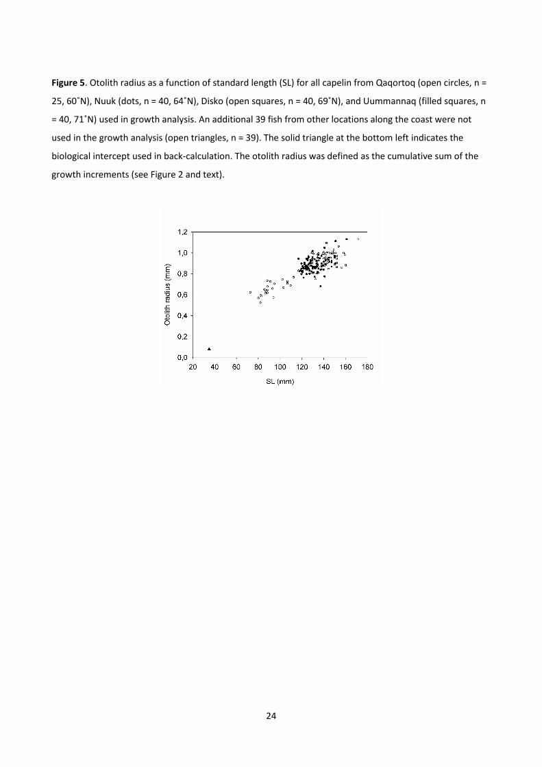
24
Figure 5. Otolith radius as a function of standard length (SL) for all capelin from Qaqortoq (open circles, n =
25, 60˚N), Nuuk (dots, n = 40, 64˚N), Disko (open squares, n = 40, 69˚N), and Uummannaq (filled squares, n
= 40, 71˚N) used in growth analysis. An additional 39 fish from other locations along the coast were not
used in the growth analysis (open triangles, n = 39). The solid triangle at the bottom left indicates the
biological intercept used in back-calculation. The otolith radius was defined as the cumulative sum of the
growth increments (see Figure 2 and text).

25
Figure 6. Somatic growth (in millimetres) of capelin from Qaqortoq (dots, n = 25, 60˚N), Nuuk (triangles, n =
40, 64˚N), Disko (squares, n = 40, 69˚N), and Uummannaq (crosses, n = 40, 71˚N). Growth was estimated
from the back-calculated lengths using the biological intercept method. Lines represent the exponential
trend lines for each area, with Qaqortoq the solid line, Nuuk the long-dashed line, Disko the short-dashed
line, and Uummannaq the dotted line.

26
Figure 7. Average temperatures for 20–50 m averaged from 1908 to 2007 for West Greenland waters (60–
73˚N 44–57˚W) from the ICES database (see text). Only measurements east of the shelf break on the west
coast of Greenland were used (<500 m). Top left, data from all months and years (n = 18 753); top right,
data for July (n = 4 671); bottom left, data for August (n = 1 632); bottom right, data for September
(n = 808). Error bars represent the standard error based on the mean values of all years at the latitudes
evaluated (n = 28–71). The areas where fish were sampled for the growth analysis are noted at their
respective latitude (see text).

27
Figure 8. Average salinity in August for 20–50 m averaged over the period 1908–2007 for West Greenland
waters (60–73˚N 44–57˚W) from the ICES database (see text). Only measurements east of the shelf break
on the west coast of Greenland (<500 m) were used (n = 1 362).

Paper III
Energy content and fecundity of capelin (Mallotus villosus) along a 1500 km
latitudinal gradient
R. Hedeholm, P. Grønkjær and S. Rysgaard
Submitted to Marine Biology

1
Energy content and fecundity of capelin (Mallotus villosus) along a 1500 km
latitudinal gradient.
1,2Hedeholm R.* 1Grønkjær P. and 2Rysgaard S.
1Marine Ecology, Department of Biological Sciences, Aarhus University. Building 1135, Ole Worms allé 1,
8000 Århus C, Denmark.
2 Greenland Climate Research Centre, c/o Greenland Institute of Natural Resources, PO Box 570, 3900
Nuuk, Greenland
*Author to whom correspondence should be addressed. Tel.: +45 8942 4392; fax: +45 8942 4387; email:
Abstract
Capelin is a planktivorous key fish species in many subarctic ecosystems representing the link between
lower trophic levels and apex predators. Little is known, however, of capelin in Greenland waters, but it
has been suggested that size and growth increases due to difference in food availability and temperature
conditions along a 1500 km south-north gradient on the west coast. It is presently unknown how the
qualitative state of capelin energy content is affected along this gradient. Based on 2007 and 2008 samples
we show that energy content increases with capelin length in both spawning and non-spawning fish, and
that it varies with latitude in spawning fish along West Greenland (60-71˚N). Combining our results on
energy content with information on capelin growth along the same latitudinal climate gradient
demonstrates that less and lower-quality food is available to capelin predators in the south than in the
north.

2
Introduction
Capelin (Mallotus villosus, Osmeridae) is a planktivorous fish with a northern circumpolar distribution.
Similar to other planktivorous species in the “wasp-waist species” guild (i.e. sardines, anchovy, sprat etc.,
Cury et al., 2000; Bakun, 2006) capelin have a life cycle characterised by a short lifespan, high mobility, high
energetic need (as a result of their numbers and high growth rates) and variable cohort strength (Gjøsæter
and Loeng, 1987; Frank and Carscadden, 1989; Carscadden et al., 2001; Gjøsæter et al., 2002; Vilhjalmsson,
2002). These characteristics can result in a fluctuating population biomass on a short time scale as
demonstrated for both capelin (Gjøsæter, 1998; Vilhjalmsson, 2002) and sardine-anchovy systems across
world oceans (Schwartzlose et al., 1999).
In Greenland, capelin is found on both the east and west coast extending north to 73˚N and 66˚N,
respectively (Friis-Rødel and Kanneworff, 2002). On the West coast this covers a 1,500 km unbroken
latitudinal gradient making capelin in this region a perfect candidate for studying the effects of changes in
environmental and climatic conditions. Capelin sensitivity to environmental changes is evident both
historically and presently. In the relatively warm 1930s capelin distribution extended as far north as 76˚N
and at the same time showed reduced abundance in southern Greenland (Jensen, 1939). Currently
sustained spawning is limited to the area south of 72˚N. More recently, changes in life history
characteristics such as growth and feeding behavior along the distributional range of capelin have been
shown (Hedeholm et al. 2010, Hedeholm et al. 2010, submitted manuscript), underlining the applicability of
capelin in this region as a model species for studying the effect of (future) environmental changes
(Anonymous, 2005) and spatial differences in vital life history characteristics such as fecundity, energy
allocation, condition and productivity.
Ecosystem-wide impacts of capelin, and wasp-waist species in general, have been shown theoretically
(Rice, 1995; Jordan et al., 2005) and the effect of a capelin-deprived diet has been shown for Canadian cod
(Rose and O'Driscoll, 2002) and in relation to the Junk-Food hypothesis in sea birds (Romano et al., 2006).
In Greenland waters the importance of capelin as prey has been demonstrated in marine mammals
(Angantyr and Kapel, 1990; Neve, 2000), cod (Gadus morhua, Nielsen and Andersen, 2001), Greenland
halibut (Reinhardtius hippoglossoides, Woll and Gundersen, 2004) and sea birds (Falk and Durinck, 1993;
Phillips et al., 1999). In all cases, capelin constituted a substantial part of the diet. Due to its lipid content
capelin has a high energy density compared to other species (Montevecchi and Piatt, 1984; Lawson et al.,
1998), and, thus, the importance of capelin is not only related to abundance, but also to tissue
composition, which determines the nutritional value of this important prey species. However, the energy
density and possible latitudinal trends for Greenlandic capelin are unknown, and satisfactory energy flow
calculations including this key species cannot be developed.

3
In this study, we provide the first area-specific data on energetic densities, fecundity and reproductive
investment for West Greenlandic capelin. As stomach content and growth rates have been shown to
increase with latitude in this area (Hedeholm et al. 2010, Hedeholm et al. 2010, submitted manuscript) two
scenarios are possible. (1) Either the observed increase in food intake is all used for growth or (2) there is
an increase in the energetic storage as well. Hence, as a null hypothesis for non-spawning capelin, we
suggest that there is no increase in energy density with increasing latitude and thus no relationship
between latitude and tissue energy density. In spawning fish all accessible tissue energy will be converted
to gonads as Greenland capelin are most likely semelparous (Friis-Rødel and Kanneworff, 2002).
Consequently, tissue energy density should not vary with latitude but be markedly reduced relative to non-
spawning individuals; a non-trivial point in constructing biomass-based energetic models. Knowledge of
Greenlandic capelin is scarce, and the present analysis will be useful in modeling (Fiksen et al., 1995).
Additionally, if capelin displays a latitudinal gradient in nutritional value similar to those shown for growth,
the impact of future climate changes may be more pronounced than previously thought.
Materials and methods
Sampling
Capelin were collected during 2007 and 2008 along the West coast of Greenland (Figure 1). Non-spawning
capelin were collected in both years by RV “Paamiut” during yearly shrimp and fish surveys conducted by
the Greenland Institute of Natural Resources. In 2007, sampling was done from 13 June to 9 September and
in 2008 from 19 June to 8 August. This stratified random bottom trawl survey covered the continental shelf
from the southern tip of Greenland to 72˚N on the West coast. The survey was done using a bottom trawl
with a vertical opening of 14 m and a towing speed of 2.5 knots. The trawl was not aimed at capelin but
these were occasionally caught, most likely during trawl haul in. All capelin caught were frozen immediately
after capture. At stations where the catch exceeded 150 individuals a random subsample of 50 individuals
was taken.
Spawning capelin were only sampled in 2007. The samples were collected during beach spawning events in
five general areas spanning 1300 km along the Greenlandic West coast: Qaqortoq (60˚00N), Nuuk (64˚00N),
Sisimiut (66˚50N) Disko (69˚00N) and Uummannaq (71˚00N, Figure 1). As spawning is temporally displaced
along the coast (Kanneworff, 1967), samples were collected later in the north than in the south, and
sampling took place from 11 May to 19 July. Samples of both spawning and non-spawning capelin were
frozen at -20 ˚C immediately after capture (see Table 1).

4
Physical measurements and fecundity
Capelin were measured to the nearest mm below (fork length) and weighed to the nearest 1/10 g. No
correction was made for shrinkage due to freezing. All spawning fish were sexed based on morphological
characteristics. This was not done for non-spawning fish as sexes appear similar prior to spawning. Gonads
were removed from spawning females, blotted dry and weighed to the nearest 1/1000 g. Fish that had
released eggs into the body cavity were excluded from analysis as some eggs may already have been
spawned.
20-60 eggs from the posterior part of the right gonad were weighed and counted, as the left gonad is
known to be underdeveloped (Winters, 1971). Based on this and total gonad weight fecundity was
calculated assuming that no difference existed between various parts of the gonad (Huse and Gjøsæter,
1997).
Energy measurements
Muscle tissue (mean ± SE = 1.09 ± 0.03 g) was removed dorsally from both sides of the fish posterior to the
dorsal fin to ensure that no bones were present. All skin was subsequently removed. Muscle tissue from all
fish and gonads from spawning females were freeze dried for 24 hours after which no further weight loss
took place. The tissue samples were weighed (dry weight, dw) and the water content was calculated (% of
wet weight, ww). Prior to any further analysis the samples were kept in an exsiccator over a dry silica gel.
The tissue samples were homogenized to a fine powder using a glass mortar and compressed into pellets of
at least 25 mg. The energy density of the pellets was determined using an 1109a semimicro bomb and Parr
6725 bomb calorimeter (Parr Instruments, Moline, USA). The bomb was calibrated with benzoic acid
(energy density: 26.454 kJ g-1) with regular intervals, and triplicates of randomly chosen samples
demonstrated low variation between samples (<2%). Energy densities differing to a large extent from other
values were reanalysed. Energy density in wet samples (reported as: kJ g ww-1) is reported in some aspects
of the study while energy density in dry samples was used in most analyses (kJ g dw-1). From an ecological
perspective the wet mass values may be more relevant (Anthony et al., 2000) but do not form the main
focus of this study as energy density expressed on a dry weight basis are more appropriate for comparative
purposes, as the variation caused by desiccation is minimized (Hislop et al., 1991). Additionally, wet mass
values are easily calculated by multiplying dry mass energy density (kJ g dw-1) by the proportion of dry mass
to wet mass. Freeze dried muscle tissue from five fish was incinerated for 24 hours at 550˚C to determine
the ash content of the samples, and energy density was calculated based on these values (kJ g ash free dw-
1). Samples from gonads were analyzed using the same procedure.

5
Lastly, data on water content, energy density and fecundity enabled calculation of individual egg energy
content, and, consequently, calculation of total energetic investment of the individual fish. The relative
reproductive investment of each fish was calculated as the amount of energy in the gonads relative to total
fish energy content (gonads excluded), under the assumption that the muscle energy density was
representative of the entire fish.
Analysis
Spawning and non-spawning fish were analyzed separately. All fish were assigned to the nearest 0.5
latitudinal degree and to one of five locations: Qaqortoq (60-61˚N), Nuuk (63-64˚N), Sisimiut (66-67˚N),
Disko (68.5-70˚N) and Uummannaq (71-72˚N, see Figure 1) to for the purpose of ANOVA-based tests.
However, Sisimiut was excluded from most statistical analyses concerning non-spawning fish, as few fish
were caught in this area. Analyses on spawning fish only include males unless stated otherwise, as
spawning females were sampled only in Nuuk. All analyses were carried out using SPSS (Statistical Package
of Social Sciences). Standard parametric tests were preceded by tests for assumptions. When these were
violated, the data were either transformed or non-parametric statistics were applied.
Results
Energy densities of 259 fish (124 spawning and 135 non-spawning) and 18 female gonads were determined
(Table 1). As no difference in energy density (kJ g dw-1) was found between 2007 and 2008 for spawning
fish (ANCOVA, F(1,128) = 0.006, P = 0.94) irrespective of both size and capture location the two years were
pooled.
Latitudinal and length effect
In non-spawning capelin there was a significant effect of both area (ANCOVA, F(3,122) = 3.573, P = 0.016) and
length (ANCOVA, F(1,122) = 26.903, P < 0.0005) on energy density, but also a significant interaction between
the two (ANCOVA, F(3,122) = 4.084, P = 0.008, Figure 2). The interaction was caused by Disko and removing
this area from the analysis yielded non-significant interaction and area terms (ANCOVA, F(2,98) = 2.105, P =
0.127 and F(1,98) = 34.768, P = 0.172, respectively). Using the parameter estimates (following model
reduction), the overall length effect and difference between the three similar areas (Qaqortoq, Nuuk and
Uummannaq) and Disko can be depicted as shown in Figure 3. A clear positive relationship between length
and energy density was seen for the pooled areas, while size effects in the Disko area were positive but
insignificant.

6
No length effect was seen in the individual areas in spawning capelin (Linear regression, P≥0.08). However,
combining areas and thereby increasing the length span, gave a significant effect of length (Linear
regression, r2 = 0.58, F1,16=8.243, P=0.028) under the assumption that the single outlier (]110-115]) can be
disregarded. This was done as this point was based on a single fish from Nuuk. The data did not allow
parametric statistics in area comparisons. Disregarding length, all but one of ten (Nuuk and Uummannaq,
P=0.89) intergroup comparisons were significant (Mann-Whitney, P≤0.034) but the most noticeable
distinction was between high values at Disko and low values at Qaqortoq (mean ± SD = 21.87 ± 0.60 kJ g dw-
1 and 20.86 ± 0.29 kJ g dw-1, respectively, Figure 4).
Spawners vs. non-spawners
Irrespective of size and location, a mean difference of 0.286 kJ g dw-1 was found in energy density (based
on dry weight, kJ g dw-1) between spawners and non-spawners (ANCOVA, F(1,248) = 248.362, P < 0.0005,
Figure 2). However, when comparisons were based on wet weight (kJ g ww-1), the non-spawning fish had
energy densities ranging from 4-4.5 kJ g ww-1 (mean ± SD = 4.32 ± 0.29 kJ g ww-1) whereas spawning fish
had much lower densities (mean ± SD = 3.68 ± 0.28 kJ g ww-1, Figure 5). The pattern was seen for all
individual areas but most clearly in Uummannaq with a difference of more than 1 kJ g ww-1 in comparable
weight groups. This discrepancy between dry and wet weight based comparison was caused by a significant
difference in water content between spawners and non-spawners, irrespective of length (mean ± SD = 82.7
± 1.11 % and 79.4 ± 1.02 %, respectively, ANCOVA, F(1,199) = 452.713, P < 0.0005).
Temporal effect
Because samples were taken in the summer feeding period, time of capture could possibly affect the
results, as energetic reserves can be expected to build during summer months, thus increasing energy
density. In general, for all non-spawning fish, there was no effect of time-of-capture on energy density over
a period of 59 days (Spearman’s correlation, rs=-0.093, N = 135, P=0.285). In the individual areas, the
sampling time span enabled such analyses in three cases (Nuuk, Qaqortoq and Disko). In the latter two no
effect of time of capture was seen (P ≥ 0.40) while a weak positive correlation was seen in Nuuk
(Spearman’s correlation, rs=0.900, N = 39, P=0.037). Here sampling took place over 14 days starting from 29
July and showed an average increase from 20.6 kJ g dw-1 to 21.6 kJ g dw-1.
In spawning capelin, a temporal development in energy density was seen in the Nuuk area, which was the
only area where such an analysis was possible as sampling took place over a period of 33 days. The energy
density decreased from 22.37 kJ g dw-1 to 21.24 kJ g dw-1 (ANCOVA, F(4,25) = 5.044, P = 0.004), while no
change in size was seen during the same period (ANCOVA, F(1,25) = 1.279, P = 0.27).

7
Sex effect
A test of differences in energy density between sexes in spawning capelin was restricted to Nuuk, as
spawning females were absent in samples from other areas. In general, energy density increased with size
(kJ g dw-1, ANCOVA, F(1,57) = 19.385, P < 0.0005, Figure 6). A difference was also found between the sexes
(ANCOVA, F(1,57) = 4.893, P = 0.031) but a significant interaction (ANCOVA, F(1,57) = 5.366, P = 0.024) made
comparisons across the sampled length range ambiguous. Within the overlapping size range (115-132mm),
no difference was found between sexes when pooling all individuals based both on dry (kJ g dw-1, Student’s
t-test, t20.25 = -0.216, P = 0.83) and wet mass (kJ g ww-1, Student’s t-test, t30 = 0.112, P = 0.91).
Fecundity and reproductive investment
Fecundity increased with gutted weight (range: 3745-11317 eggs, regression, r2 = 0.69, F1,16 = 35.955, P <
0.0001) and the relationship was best described as: Fecundity = 356.63 * gutted weight1.4414, Figure 7). On
average the female gonads contained (mean ± SD) 37.8 ± 3.3 % of total female capelin energy, and
reproductive investment was positively related to weight (Linear regression, r2 = 0.36, F1,16 = 8.912, P =
0.009, Figure 7) as was the gonadosomatic index (Linear regression, r2 = 0.35, F1,16 = 19.176, P < 0.0005, data
not shown). The individual egg energy content was (mean ± SD) 2.67 ± 0.36 J but was not related to weight
(Spearman’s correlation, rs=0.176, N = 18, P = 0.486).
Discussion
To our knowledge, this study represents the first data on energy density for Greenlandic capelin. The
densities (based on dry matter, kJ g dw-1) are lower than seen in other studies (e.g. Jangaard, 1974; Lawson
et al., 1998; Anthony et al., 2000). As these studies demonstrate higher energy densities than shown here,
spatial differences may exist. However, most other studies convert proximate composition to energy
density, thus relying on energetic conversion factors, and often use low conversion factors for protein
include only assimilable energy (17.8-20.0 kJ g dw-1). Converting values given by Anthony et al. (2000) on
Alaskan capelin to energetic densities using an energy equivalent of 23.2 kJ g dw-1 for protein (as
determined in this study using reference material) we find an energy density of 26.6 kJ g ash free dw-1 in
non-spawning capelin compared to 22.3 kJ g ash free dw-1 in this study (the ash content of capelin was
5.72%). Similarly, Montevecchi and Piatt (1984) present results from Newfoundland, Canada, with non-
spawning capelin having re-calculated energy densities of 24-29 kJ g dw-1 similar to those presented by
Jangaard (1974) and Lawson et al. (1998). As calculations in the mentioned studies, and other energetic
studies on fish (e.g. Van Pelt et al., 1997; Ball et al., 2007), are made from proximate fish composition, the

8
difference may be a result of differences in methodology (i.e. lipid extraction) causing overestimation
(Jezierska, 1974; Craig et al., 1978). Other studies using bomb calorimetry on pelagic fishes obtain values
much like those showed here (e.g. Smith et al., 1990; Kitts et al., 2004) and we believe that the values are
accurate, but if they are to be used in energetic budgets of capelin predators, correcting for efficiency of
the metabolic pathway is needed (Ball et al. 2007).
Lastly, the timing of the samples collected in this study may partly explain the difference, as a seasonal
change in proximal composition, and thus energy density, of capelin has been reported from other waters
(Jangaard, 1974; Eaton et al., 1975; Montevecchi and Piatt, 1984; Lawson et al., 1998 and references;
Anthony et al., 2000) as well as in other fishes (e.g. Hislop et al., 1991; Schwarz and Hammer, 1996; Kitts et
al., 2004) with a minimum in the mid summer months because of a bimodal production cycle. Hence,
Jangaard (1974) observed an increase from 21.2 kJ g dw-1 in June/July to 26.7 kJ g dw-1 in August in
Canadian capelin (determined from proximate fish composition).
The “energy density/water” ratio changes due to reciprocal substitution of tissue and water as the tissue is
metabolized. Anthony et al. (2000) used water content in capelin as a proxy for energy content explaining
97% of the variation (based on energy density in wet mass), and Jangaard (1974) found a peak in water
content of 82%, to be coincident with the lowest energy density. As the mean water content in this study
was 80%, a matching low energy density may be expected. In general, we saw no effect of time of capture
on energy density, but in Nuuk there was a 1 kJ g dw-1 increase over time in non-spawning fish, suggesting
that sampling throughout the season is necessary to allow detailed comparison with other studies.
Latitudinal and length effects
There was no evidence of a clear latitude-related trend in energetic density in non-spawning capelin. As
growth increases along the same latitudinal gradient (Hedeholm et al. 2010) this indicates that the increase
in energy intake with latitude is all converted to growth, and not stored as energy. However, there was a
large difference between Qaqortoq and Disko in spawning fish (20.86 and 21.87 kJ g dw-1, respectively),
which are also the two areas showing the largest growth differences, indicating that these areas represent
the southern distributional limit where environmental constraints limit capelin growth (Qaqortoq) and the
optimal living conditions (Disko), respectively. Hence, the decline in energy density in Uummannaq north of
Disko may represent the early signs of a northern distributional limit and the decrease is again similar to
that observed in capelin growth. Indeed, the latitudinal gradient in growth may be viewed as energy
storage in terms of increased somatic mass, which serves as a positive fitness parameter in that the
reproductive investment was found to be positively related to length (Fig. 7). However, the possibility of a
temporal artifact needs to be considered, as energy density in Nuuk was shown to decline with almost 1 kJ

9
g dw-1 over a one-month period. This needs to be confirmed with sampling on a finer temporal scale along
the latitudinal gradient.
There was a clear general increase in energy density (kJ g dw-1) with size in non-spawning capelin in three
(Qaqortoq, Nuuk and Uummannaq) of the four analyzed areas (Sisimiut excluded, Figure 2). The reason for
the inconsistency in the Disko area, where only a slight increase in energy density with length was seen, is
unknown. However, the analyzed size spectrum is smaller in this area and the inclusion of smaller
individuals may have resulted in an increase similar to that seen in other areas.
The positive relationship between size and energy density is similar to that shown in Alaskan capelin
(Anthony et al., 2000) as well as other pelagic species (Hislop et al., 1991). This length-related difference in
nutritional value in interaction with similar latitudinal growth variation may have an important impact on
higher trophic levels depending on capelin (Lavigne et al., 1985; Falk and Durinck, 1993; Nielsen and
Andersen, 2001). As the average length-at-age increases by more than 50% across the latitudinal gradient,
changes in capelin growth conditions may have a large effect on the ecosystem (Carscadden et al., 2001) as
energetic densities can be expected to change accordingly – further emphasized by the fact that a
reduction in size not only reduces energy density but also energy intake, as capelin weight can be expected
to decrease by 87% with a 50% length reduction (Hedeholm et al., 2010). Faced with climate change
(Holland and Bitz, 2003) and a partly temperature-controlled growth pattern (Gjøsæter and Loeng, 1987;
Hedeholm et al., 2010) such changes are likely to occur in Greenlandic waters (Huse and Ellingsen, 2008)
and they will affect energy flow (Carscadden et al., 2001) and probably species distribution (Drinkwater,
2005).
Although less clear, there was also a length effect on energy density in male spawning capelin. Capelin
spawning takes place in shallow waters (Friis-Rødel and Kanneworff, 2002) forcing capelin into large easily
accessible shoals during this period, and it is during this period that they are preyed heavily upon by cod,
seabirds, whales and seals. Hence, the latitudinal growth (Hedeholm et al. 2010) and energy density (this
study) gradients present along the Greenlandic west coast indicate that increasing temperatures will
increase both capelin size and energy density, providing better feeding conditions for many predators. This
is, however, dependent on temperatures staying within the optimal range and food being sufficient to
meet metabolic demand.
The energy density was similar to that of non-spawning capelin based on dry mass (mean ± SD = 21.4 ± 0.5
kJ g dw-1), but differed significantly based on wet mass (mean ± SD = 3.44 ± 0.97 kJ g ww-1) because of a
significant difference in water content (Figures 2 and 5). This leads to the conclusion that as spawning
approaches, feeding is reduced (O'Driscoll et al., 2001) and tissue is broken down and progressively
replaced by water, while remaining tissue maintains the same composition until metabolized. The decline
10
in energy content with time in male spawning capelin is consistent with knowledge on capelin spawning
behavior. Males stay on the spawning grounds for longer periods awaiting small schools of females
(Vilhjálmsson, 1994), and to support metabolism in this period of limited food intake (Templeman, 1948; R.
Hedeholm, pers. obs.), tissue must be metabolized.
Fecundity and reproductive investment
Fecundity estimates (mean ± SD = 6185 ± 2249 eggs) were much lower than estimates from the Barents Sea
(approx. 11000, e.g. Gjøsæter and Monstad, 1973; Huse and Gjøsæter, 1997), Pacific (approx. 20000,
Velikanov, 2002) and Canada (>20000, Nakashima, 1987). However, as all studies (the present one
included) show positive fecundity-size relationships (Figure 7), the size-specific fecundity in this study is as
high or higher than in other studies (converting fork length to total length using a conversion factor of
1.08).
The reproductive investment was high (38%), which was as expected for a – to a varying degree –
semelparous species and corresponds well with the semelparous/iteroparous limit of 60% (migration and
spawning) suggested by Glebe and Leggett (1981). Hence, values of 10-30% have been demonstrated for
iteroparous species such as Arctic charr (Jonsson and Jonsson, 1997; Finstad et al., 2002) and Atlantic cod in
Greenland (Hedeholm et al., unpublished manuscript).
Reproductive investment increased with weight, but individual egg energy content (mean ± SD = 2.67 ±
0.36 J) did not. This has several possible explanations. The increase in investment could simply be a result
of body cavity volume increasing more with a given weight increase (i.e. higher fecundity) than somatic
energy content or that smaller fish have a higher proportion of essential tissue that is not convertible to
gonads. However, it could also reflect a need to conserve more energy in smaller capelin as a response to
an iteroparous life history strategy, which has been suggested for female capelin (Sørensen, 1985;
Vilhjálmsson, 1994; Huse, 1998; Friis-Rødel and Kanneworff, 2002). In iteroparous species it might be
expected that first time spawners produce lower quality eggs or/and invest less in reproduction than more
experienced individuals (Trippel, 1998; Carr and Kaufman, 2009). This study supports the latter of these
notions and encourages further research on both male and female capelin.

11
References
Anonymous (2005) Arctic Climate Impact Assessment, Cambridge University Press. 1042pp
Angantyr LA, Kapel FO (1990). Harp seal feeding habits in Greenland - our present knowledge, April 1990.
Technical Report of the Greenland Fisheries Research Institute: 72
Anthony JA, Roby DD, Turco KR (2000) Lipid content and energy density of forage fishes from the northern
Gulf of Alaska. J Exp Mar Biol Ecol 248:53-78
Bakun A (2006) Wasp-waist populations and marine ecosystem dynamics: Navigating the "predator pit"
topographies. Prog Oceanogr 68:271-288
Ball JR, Esler D, Schmutz JA (2007) Proximate composition, energetic value, and relative abundance of prey
fish from the inshore eastern Bering Sea: implications for piscivorous predators. Pol Bio 30:699-708
Carr JP, Kaufman L (2009). Estimating the importance of maternal age, size, and spawning experience to
recruitment of Atlantic cod (Gadus morhua). Bio Cons 142:477-487
Carscadden JE, Frank KT, Leggett WC (2001) Ecosystem changes and the effects on capelin (Mallotus
villosus), a major forage species. Can J Fish Aquat Sci 58:73-85
Craig JF, Kenley MJ, Talling JF (1978) Comparative Estimations of the Energy Content of Fish Tissue from
Bomb Calorimetry, Wet Oxidation and Proximate Analysis. Fresh Bio 8:585-590
Cury P, Bakun A, Crawford RJM, Jarre A, Quinones RA, Shannon LJ, Verheye HM (2000) Small pelagics in
upwelling systems: patterns of interaction and structural changes in "wasp-waist" ecosystems. ICES J Mar
Sci 57:603-618
Drinkwater KF (2005) The response of Atlantic cod (Gadus morhua) to future climate change. ICES J Mar Sci
62:1327-1337
Eaton CA, Ackman RG, Tocher CS, Spencer KD (1975) Canadian Capelin 1972-1973 - Fat and Moisture
Composition, and Fatty-Acids of Some Oils and Lipid Extract Triglycerides. J Fish Res Board Can 32:507-513
Falk K, Durinck, J (1993) The Winter Diet of Thick-Billed Murres, Uria-Lomvia, in Western Greenland, 1988-
1989. Can J Zool 71:264-272
Fiksen O, Giske J, Slagstad D (1995) A Spatially Explicit Fitness Based Model of Capelin Migrations, the
Barents Sea. Fish Oceanogr 4:193-208
Finstad AG, Berg OK, Langeland A, Lohrmann A (2002) Reproductive investment and energy allocation in an
alpine Arctic charr, Salvelinus alpinus, population. Environ Biol Fishes 65:63-70
Frank KT, Carscadden JE (1989) Factors Affecting Recruitment Variability of Capelin (Mallotus-Villosus) in
the Northwest Atlantic. ICES J Mar Sci 45:146-164
Friis-Rødel E, Kanneworff P (2002) A review of capelin (Mallotus villosus) in Greenland waters. ICES J Mar
Sci 59:890-896

12
Gjøsæter H (1998) The population biology and exploitation of capelin (Mallotus villosus) in the Barents Sea.
Sarsia 83:453-496
Gjøsæter H, Dalpadado P, Hassel A (2002) Growth of Barents Sea capelin (Mallotus villosus) in relation to
zooplankton abundance. ICES J Mar Sci 59:959-967
Gjøsæter H, Loeng H (1987) Growth of the Barents Sea Capelin, Mallotus Villosus, in Relation to Climate.
Environ Biol Fishes 20:293-300
Gjøsæter H, Monstad T (1973) Fecundity and egg size of spring spawning Barents sea capelin. FiskDir Skr
(Ser Havunders) 16:98-104
Glebe BD, Leggett WC (1981) Temporal, Intra-Population Differences in Energy Allocation and Use by
American Shad (Alosa-Sapidissima) During the Spawning Migration. Can J Fish Aquat Sci 38:795-805
Hedeholm R. Grønkjær P, Rysgaard S (2010) Differentiated growth of Greenlandic capelin (Mallotus villosus
Müller) along a latitudinal gradient. ICES J Mar Sci, In press.
Hislop JRG, Harris MP, Smith JGM (1991) Variation in the Calorific Value and Total Energy Content of the
Lesser Sandeel (Ammodytes-Marinus) and Other Fish Preyed on by Seabirds. J Zool 224:501-517
Holland MM, Bitz CM (2003) Polar amplification of climate change in coupled models. Clim Dyn 21:221-232
Huse G (1998) Sex-specific life history strategies in capelin (Mallotus villosus)? Can J Fish Aquat Sci 55:631-
638
Huse G, Ellingsen I (2008) Capelin migrations and climate change - a modelling analysis. Clim Change
87:177-197
Huse G, Gjøsæter H (1997) Fecundity of the Barents Sea capelin (Mallotus villosus). Mar Biol 130:309-313
Jangaard PM (1974) The capelin (Mallotus villosus). Biology, distribution, exploitation, utilization and
composition. Fish Res Bd Can Bull 186:1-70
Jensen AS (1939) Concerning a change of climate during recent decades in the Arctic and subarctic regions,
from Greenland in the west to Eurasia in the east and contemporary biological and geophysical changes.
Meddelelser om Grønland, 8.
Jezierska B (1974) The effect of various type of food on the growth and chemical composition of the body
of perch (Perca fluviatilis L.) in laboratory conditions. Pol Arch Hydrobiol 21:467-479
Jonsson N, Jonsson B (1997) Energy allocation in polymorphic brown trout. Func Ecol 11:310-317
Jordan F, Liu WC, Wyatt T (2005) Topological constraints on the dynamics of wasp-waist ecosystems. J Mar
Syst 57:250-263
Kanneworff P (1967) Mallotus villosus (O. F. Müller). Biologi og dynamik i grønlandske farvande. [Mallotus
villosus (O. F. Müller). Biology and dynamics in Greenland waters]. Thesis, Grønlands Fiskeriundersøgelser.
Copenhagen: 103 pp.
13
Kitts DD, Huynh MD, Hu C, Trites AW (2004) Season variation in nutrient composition of Alaskan walleye
pollock. Can J Zool/Rev Can Zool 82:1408-1415
Lavigne DM, Innes S, Stewart REA, Worthy GAJ (1985) An annual energy budget for north-west Atlantic
harp seals. In Marine mammals and fisheries. J. R. Beddington, R. J. H. Beverton and D. M. Lavigne: 319-335.
Lawson JW, Magalhaes AM, Miller EH (1998) Important prey species of marine vertebrate predators in the
northwest Atlantic: proximate composition and energy density. Mar Ecol Prog Ser 164:13-20
Montevecchi WA, Piatt J (1984) Composition and Energy Contents of Mature Inshore Spawning Capelin
(Mallotus-Villosus) - Implications for Seabird Predators. Comp Biochem Physiol A: Mol Integr Physiol 78:15-
20
Nakashima BS (1987) Regional and temporal variations in fecundity of capelin in Newfoundland waters. T
Am Fish Soc 116:864-873
Neve PB (2000) The diet of the minke whale in Greenland - A short review. Minke Whales, Harp and
Hooded Seals: Major Predators in the North Atlantic Ecosystem. NAMMCO Scientific Publications 2:92-96
Nielsen JR, Andersen M (2001). Feeding habits and density patterns of Greenland cod (Gadus ogac)
(Richardson 1836), at West Greenland compared to those of the coexisting Atlantic cod, Gadus morhua L. J
Northwest Atl Fish Sci 29:1-22
O'Driscoll RL, Parsons MJD, Rose GA (2001) Feeding of capelin (Mallotus villosus) in Newfoundland waters.
Sarsia 86:165-176
Phillips RA, Petersen MK, Lilliendahl K, Solmundsson J, Hamer KC, Camphuysen CJ, Zonfrillo B (1999) Diet of
the northern fulmar Fulmarus glacialis: reliance on commercial fisheries? Mar Biol 135:159-170
Rice J (1995) Food web theory, marine food webs, and what climate change may do to northern marine fish
populations. In Climate change & Northern fish populations. R. J. Beamish, Canadian special Publications of
Fisheries and Aquatic Sciences. 121: 561-568.
Romano MD, Piatt JF, Roby DD (2006) Testing the junk-food hypothesis on marine birds: Effects of prey
type on growth and development. Waterbirds, 29(4): 407-414.
Rose GA, O'Driscoll RL (2002) Capelin are good for cod: can the northern stock rebuild without them? ICES J
Mar Sci 59:1018-1026
Schwartzlose, R. A., et al. 1999. Worldwide large-scale fluctuations of sardine and anchovy populations. S
Afr J Mar Sci-S-Afr Tydskr Seewe 21:289-347
Schwarz G, Hammer C (1996) Size and seasonal effects on the body calorific content of North Sea whiting
(Merlangius merlangus L, Gadidae). Arch Fish Mar Res 44:33-46
Smith RL, Paul AJ, Paul JM (1990) Seasonal-Changes in Energy and the Energy-Cost of Spawning in Gulf of
Alaska Pacific Cod. J Fish Biol 36:307-316

14
Sørensen EF (1985) Ammassat ved Vestgrønland [Capelin at West Greenland], Fiskeri- og
Miljøundersøgelser i Grønland: 82.
Templeman W (1948) The life history of the capelin (Mallotus villosus O. F. Müller) in Newfoundland
waters. Research Bulletin of the Newfoundland Government Laboratory, 17: 151.
Trippel EA (1998) Egg size and viability and seasonal offspring production of young Atlantic cod. T Am Fish
Soc 127:339-359
Van Pelt TI, Piatt JF, Lance BK, Roby DD (1997) Proximate composition and energy density of some North
Pacific forage fishes. Comp Biochem Physiol A: Mol Integr Physiol 118:1393-1398
Velikanov AY (2002) Spatial differences in reproduction of capelin (Mallotus villosus socialis) in the coastal
waters of Sakhalin. ICES J Mar Sci 59:1011-1017
Vilhjalmsson H (2002) Capelin (Mallotus villosus) in the Iceland-East Greenland-Jan Mayen ecosystem. ICES
J Mar Sci, 59:870-883
Vilhjálmsson H (1994) The Icelandic Capelin Stock, Journal of the Marine Research Institute. 281 pp.
Winters GH (1971) Fecundity of Left and Right Ovaries of Grand Bank Capelin (Mallotus-Villosus). J Fish Res
Board Can 28:1029-1033
Woll AK, Gundersen AC (2004) Diet composition and intra-specific competition of young Greenland halibut
around southern Greenland. J Sea Reas 51:243-249

15
Table I
Location, number, physical data, water content (%) and energy density (kJ g dw-1) for all sampled capelin
(mean ± SD). Length and weight data in the “gonads” section refers to the fish, while the remainder refers
to the gonads. Qaqortoq: 60-61˚N, Nuuk: 63-64˚N, Sisimiut: 66-67˚N, Disko: 68.5-70˚N and Uummannaq:
71-72˚N.
Area N Length (mm) Weight (g) Water content (%) Energy density (kJ g dw-1
)
Spawning (2007)
Qaqortoq 6 120 ± 4.2 10.1 ± 1.4 82.1 ± 1.1 20.861 ± 0.287
Nuuk 61 124 ± 13.3 13.0 ± 4.5 82.5 ± 0.9 21.276 ± 0.691
Sisimiut 22 144 ± 6.3 21.8 ± 3.3 82.8 ± 1.1 21.155 ± 0.273
Disko 14 149 ± 4.6 29.9 ± 4.0 81.8 ± 1.0 21.856 ± 0.597
Uummannaq 21 145 ± 6.9 24.5 ± 4.3 84.0 ± 0.8 21.423 ± 0.340
Non-spawning (2007+2008)
Qaqortoq 41 113 ± 1.9 7.7 ± 3.9 79.7 ± 1.0 20.869 ± 0.748
Nuuk 42 122 ± 1.2 10.1 ± 3.1 79.7 ± 1.3 21.122 ± 0.691
Sisimiut 5 124 ± 0.4 10.7 ± 2.0 80.0 ± 0.6 20.984 ± 0.381
Disko 26 142 ± 1.5 16.0 ± 5.2 79.3 ± 0.6 21.276 ± 0.545
Uummannaq 24 126 ± 1.5 8.9 ± 1.7 78.7 ± 0.6 20.950 ± 0.612
Gonads (2007)
Nuuk 18 111 ± 8.9 9.5 ± 2.3 71.3 ± 1.6 24.795 ± 0.251

16
Figure 1
The southern part of Greenland with the study areas marked. The arrows mark areas where spawning
capelin were sampled in 2007. From south to north, these are Qaqortoq, Nuuk, Sisimiut, Disko and
Uummannaq. The circles mark the off-shore areas where non-spawning capelin were sampled in 2007 and
2008.

17
Figure 2
Mean energy density (kJ g dw-1) of spawning (open circles) and non-spawning (filled circles) capelin caught
in 2007 and 2008 along the Greenlandic west coast at five locations (Nspawners, Nnon-spawners): Qaqortoq (6, 41),
Nuuk (61, 42), Sisimiut (22, 5), Disko (14, 26), Uummannaq (21, 24). All areas are shown separately and
combined. The combined values are un-weighted averages. The lines in the combined graph represent
linear regression of energy density on length for both spawning (dashed, r2=0.58, P=0.03, disregarding the
]110-115] category (see text)) and non-spawning (solid, r2=0.67, P<0.0005). Bars represent standard error.

18
Figure 3
The predicted relationship and 95% confidence intervals between energy density (kJ g dw-1) and size in non-
spawning capelin from Greenland based on model parameter estimates (see text). The areas that did not
differ statistically are combined (Qaqortoq, Nuuk and Uummannaq, solid lines) while Disko is depicted
alone (dashed lines). Parameter estimates are (y=a*x+b): a=0.025; b=18.015 and a=0.004; b=20.571 for
combined areas and Disko respectively.

19
Figure 4
Mean energy density (kJ g dw-1) in male spawning capelin from five locations on the Greenlandic west
coast: Qaqortoq (60-61˚N), Nuuk (63-64˚N), Sisimiut (66-67˚N), Disko (68.5-70˚N) and Uummannaq (71-
72˚N). N is noted for each area. Bars represent standard error.
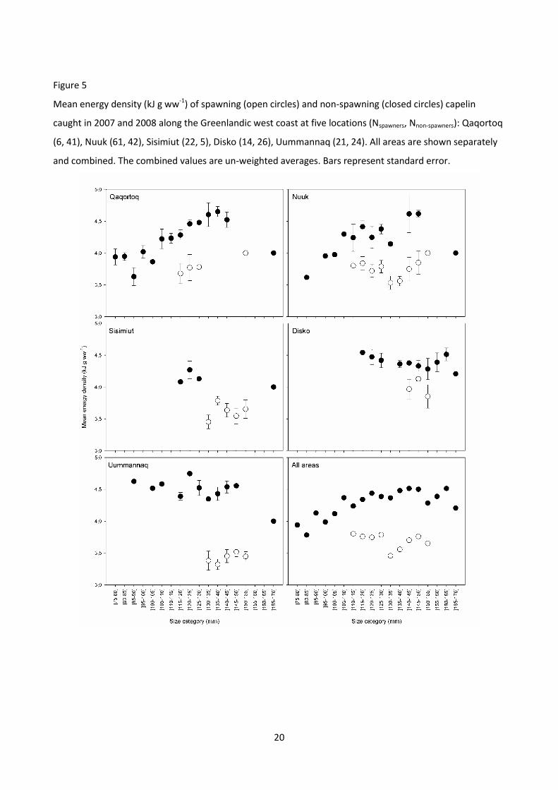
20
Figure 5
Mean energy density (kJ g ww-1) of spawning (open circles) and non-spawning (closed circles) capelin
caught in 2007 and 2008 along the Greenlandic west coast at five locations (Nspawners, Nnon-spawners): Qaqortoq
(6, 41), Nuuk (61, 42), Sisimiut (22, 5), Disko (14, 26), Uummannaq (21, 24). All areas are shown separately
and combined. The combined values are un-weighted averages. Bars represent standard error.
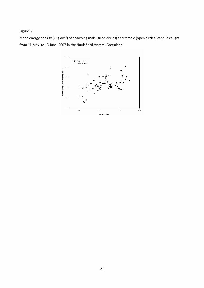
21
Figure 6
Mean energy density (kJ g dw-1) of spawning male (filled circles) and female (open circles) capelin caught
from 11 May to 13 June 2007 in the Nuuk fjord system, Greenland.

22
Figure 7
Top: fecundity of female capelin from Nuuk fjord (64˚N) as a function of gutted wet weight (N=18). The line
represents power regression (Fecundity = 356.63 * gutted weight1.4414, r2=0.69, P<0.0001).
Bottom: the relative reproductive investment (%) measured as total gonad energy relative to total fish
energy content (gonads excluded). The line represents linear regression.

Paper IV
Summer diet of inshore cod in West Greenland: importance of capelin
R. Hedeholm, K.N. Mouritsen, J. Carl and P. Grønkjær
Prepared for submission for Journal of Marine Biology

1
Summer diet of inshore cod in West Greenland: importance of capelin
1Hedeholm R.*, 1Mouritsen K.N., 2Carl J. and 1Grønkjær P.
1 Marine Ecology, Department of Biological Sciences, Aarhus University, Ole Worms allé 1, 8000 Aarhus C,
Denmark
2 Greenland Institute of Natural Resources, PO box 570, 3900 Nuuk, Greenland
*Author to whom correspondence should be addressed. Tel.:+45 8942 4392; fax: +45 8942 4387; email:
Abstract
The summer feeding ecology of Atlantic cod (Gadus morhua) was investigated in two West Greenlandic
fjord systems (Nuuk and Sisimiut fjords) in order to quantify the relative importance of different prey
species. The prey composition based on stomach content was similar in cod from both fjords, with capelin
(Mallotus villosus) being the most important prey by weight (70%) followed by “other prey” (mostly other
fish species, 12%) and crabs (8%). There were indications of an ontogenetic shift in diet with non-fish prey
(fish eggs, crustaceans) being more dominant in smaller cod below 30 cm in length (24%) while fish prey
dominated in larger cod (84%). The condition factor of cod differed between fjords being the highest in the
most northerly fjord (Sisimiut) in all size classes. In both fjords, the condition factor declined in the largest
fish. This could possibly be related to completed spawning activity. However, decreased capelin availability
during recent years may have also influenced the condition of larger cod. The latter assumption is consistent
with a demonstrated historical decline in length-at-age in larger cod.
Key words: capelin, condition factor, crustaceans, Gadus morhua, inshore, length-at-age, ontogenetic shift

2
INTRODUCTION
Atlantic cod (Gadus morhua L.) is found throughout the North Atlantic. This also includes the coast of
Greenland where it lives at the northern limit of its range (Drinkwater, 2005). Here Atlantic cod has been a
very important species for commercial fisheries in the past with catches up to 500.000 metric tons in the
late 1960’s. Subsequently, the population collapsed (Buch et al., 1994), and shortly thereafter, the yearly
catch decreased to about 50 metric tons in the 1990’s and has at present not recovered (Storr-Paulsen et
al., 2004).
Feeding behaviour, along with temperature, has been shown to affect cod condition (Rose &
O'Driscoll, 2002; Mello & Rose, 2005; Ratz & Lloret, 2005). Because there are only a few studies on feeding
habits and condition of Atlantic Cod in West Greenland (e.g. Hansen, 1949; Lloret & Ratz, 2000), more
knowledge on the feeding ecology of cod in Greenlandic waters is important from two perspectives. Firstly,
these studies could help elucidate the importance of different prey species as one step toward
understanding why cod populations have not regained their former population strengths. For instance, it
has been shown that the lipid-rich capelin (Mallotus villosus Müller) (Montevecchi & Piatt, 1984; Lawson et
al., 1998) is a key prey item for Atlantic cod in Canadian and Icelandic waters (Methven & Piatt, 1989;
Magnusson & Aspelund, 1997), and cod populations are affected by fluctuations in capelin stock size
(Marshall et al., 1999; Vilhjalmsson, 2002). Furthermore, Hansen (1949) has shown that this has also been
the case for the Atlantic cod in West Greenland in the past. Secondly, if cod once again becomes abundant
in West Greenlandic waters, knowledge of its feeding behaviour and subsequent impact on the prey
community through top down effects would be important, as a large abundance of cod will affect the
ecology of other species, including commercially exploited species such as snow crabs (Chionoecetes opilio),
deepwater shrimp (Pandalus borealis) and capelin.
Thus, to add to the knowledge of Atlantic cod’s feeding ecology in West Greenland this study
was undertaken to investigate their summer diets in inshore areas. In particular, it was of interest to
evaluate the importance of capelin in the diet of cod and describe possible ontogenetic diet shifts.
Additionally, as the inshore cod in Greenland is largely non-migratory (Storr-Paulsen et al., 2004) two
separate fjord systems were investigated to assess the possible existence of regional differences in prey
composition. A large spatial variation in prey composition might suggest that the reason for the lack of
recovery of the cod population in West Greenland would not necessarily be linked to absence of specific
key prey species.

3
MATERIALS AND METHODS
Study site and sampling
The study was carried out from June 19th to July 9th in 2005 in West Greenland, where a total of 227 Atlantic
cod were caught in two main areas: the Nuuk (Godthaab) fjord system (100 fish) and the Sisimiut
(Holsteinsborg) fjord system (127 fish). These areas are in NAFO division’s 1D (North of 6230’ and south of
6415’) and 1B (North of 68°00' and south of 68°50'), respectively.
Fish were caught using survey gillnets with five different mesh sizes (16.5, 18, 24, 28 and 33 mm) in sections
of equal length (10 m). Ten gillnets were combined to make up a total of 100 meters of net with each of the
five mesh sizes represented twice. The order of the different mesh sizes was randomized, and each net was
separated from neighbouring nets by 2 m. The nets were set 2 m off the bottom.
At each location the 100 m nets were set at a maximum depth of 20 m. Depending on
weather conditions, the nets were set to fish for 6½ - 12 hours which ensured at least one tidal cycle during
the fishing period. Due to the latitude and time of year the light intensity varied little over the course of a
day. At the end of the fishing period the nets were retrieved and all Atlantic cod were measured (total
length, LT, cm) and weighed (wet weight, W, g). With the exponent determined from length-weight
regression (3.033), the condition factor (CF) was calculated as follows:
033.3
100TL
WCF
Fish showing evidence of regurgitation (i.e. stomach content in the mouth) or having been partly eaten by
scavengers were not included in this study. Remaining fish were gutted, sexed and the stomach was
removed and frozen within one hour. The stomach was defined as the section of the alimentary canal from
the oesophagus to the pylorus sphincter.
Stomach analysis
In the laboratory, the stomachs were slowly thawed at 10 ˚C and cut open with scissors. The entire stomach
content was blotted dry and weighed and all prey was determined to the lowest possible taxonomic level
and subsequently placed into taxonomic categories accordingly.
Eleven prey species were identified and these were pooled into a total of seven prey
categories because of the rarity of some of the prey species. The category ‘large crustaceans’ contained krill
(Euphausiidae sp.) as the most dominating prey species along with the crustaceans’ deepwater shrimp and
polar lebbeid (Lebbeus polaris). The category ‘crabs’ contained snow crab and sand crab (Hyas araneus).
These two species were pooled into one category since appendages (e.g. legs) were the most commonly
eaten parts and these were often indistinguishable between species due to digestion. Taxonomic groups

4
that occurred only seldom were placed in a joint category (‘other’), which included echinoderms Asteroide
sp., bristle worms Polychates sp., cephalopods Gonatus sp., and the fish Pholis gunnellus L., and Cottidae
sp. in which the fish were the dominant species. The category ‘capelin’ consisted of adult individuals of this
species (no juveniles were found). The category ‘small crustaceans’ was made up of juvenile stages of
several crustaceans, of which juvenile crabs (primarily Chionoecetes opilio and Hyas araneus) made up the
largest fraction. ‘Unknown’ and ‘capelin eggs’ made up the two last categories (Table 1).
Prey composition was expressed as relative prey abundance (AW),
1)()( tiiW WWA
where Wi is the wet mass (g) of prey in a given category and Wti is the total wet mass (g) of prey in the
stomachs containing prey (Nielsen & Andersen, 2001).
Statistical analysis
All analyses were carried out using SPSS (Statistical Package of Social Sciences). Standard parametric tests
were preceded by test for assumptions. When these were violated, the data were either transformed or
non-parametric statistics were applied. Percentage data were arcsine-transformed prior to analyses. The
mean share of each prey group in each size group was compared between areas (e.g. capelin share
compared between Nuuk and Sisimiut etc.) yielding a total of 42 comparisons.
RESULTS
Prey composition
The cod ranged in mass from 30 to 3840 g and in length from 13 to 69 cm. The share of empty stomachs
constituted 19% of all stomachs and did not differ between the two fjords (Table 1, Fisher’s exact test,
P=0.87). Empty stomachs were excluded from further stomach analysis, however these cod were included
in the condition analysis.
The stomach content was similar between areas (Table 1). Specific size group comparisons
between areas only yielded one significant difference between areas out of 42 possible. This was within the
‘large crustaceans’ category, where there was a larger share in of this prey in cod from Nuuk than in cod
from Sisimiut (Mann-Whitney, Z31=3.552, P=0.004). However, as ‘large crustaceans’ constituted less than
1.5% of the total prey weight and this did not differ between study areas the overall prey compositions of
Nuuk and Sisimiut cod were pooled in further analyses. Further supporting a similar spatial feeding pattern
between cod in both fjords was the similarity in the relative amount of prey (standardized to fish weight) in
both fjords (Student’s t-test, t181=0.321, P=0.75, Figure 1).

5
Capelin was the dominant prey group (70% of total prey weight) while only the prey category ‘other’ also
constituted more than 10% (12%, Table 1) when all stomach contents was pooled. The relatively large
contribution from the ‘other’ prey group was due to the inclusion of large prey fish in this category. The
dominance of capelin as prey was evident in most size groups in both areas; however a decline was seen in
the largest cod in both areas coinciding with an increase in the ‘other’ prey category. Because the ‘other’
prey category is dominated by fish prey, the overall importance of fish prey appears to increase with size at
the expense of smaller prey. Hence, in the smaller cod size groups ‘small crustaceans’, ’large crustaceans’
and ’capelin eggs’ constituted a comparatively important part of the diet. The overall pattern of fish (mainly
capelin) increasing in importance as prey with increasing cod size is further supported by the contrast in the
share of fish prey and non-fish prey in small (≤30cm) and large cod (>30cm, Figure 2). However, as these
comparisons are based on prey wet weight, large fish prey will contribute considerably more to the overall
picture than small prey, even if large fish prey are present in only a small fraction of the investigated cod.
Hence, if the size related feeding behaviour is viewed as the mean share of prey groups in individual fish it
appears that smaller cod (less than 30 cm) generally do not eat fish prey, but subsist mainly on a diet of
non-fish organisms (Figure 3).
Condition factor
The condition factor (CF) of inshore cod was significantly higher in Sisimiut (mean ±SD: 0.886 ± 0.123) than
in Nuuk (0.836 ± 0.106, Student’s t-test, t225=3.251, P=0.001, Figure 4). The uncharacteristically low CF in
the 40-50 cm length group of cod from Nuuk was not caused by any outliers or lack of data points and the
reason for this inconsistency is unknown. In both areas there was a tendency for CF to decline in fish above
50 cm. Due to the unexplained low CF-value in Nuuk in the 40-50 cm size category this was most clear in
Sisimiut. However, assuming that the 40-50 cm size category was similar in both areas a decline similar to
that in Sisimiut was seen in the two largest size groups in Nuuk, suggesting an overall pattern of decreasing
CF in larger fish in both fjord systems.
DISCUSSION
The present results show that the primary food source of Atlantic cod in two West Greenland fjord systems
during the early summer is capelin, without notable differences between Nuuk and Sisimiut fjord systems.
This trend tends to increase as the cod grow larger. These results are in general agreement with previous
studies in the region (Hansen, 1949; Nielsen & Andersen, 2001). Nielsen & Andersen (2001) found that
capelin in West Greenland constituted 44% of total prey weight, which is less than what was observed in
the present study where capelin made up more than 50% of prey in most size groups and 70% in total

6
(Table 1). This discrepancy can probably be explained by differences in the sampling season. Nielsen &
Andersen (2001) sampled in November when capelin have generally migrated to deeper waters along the
coastline. In contrast, capelin gather in large numbers in the shallow waters of the fjords during spawning
in the Spring (May-June, this study) which makes them more easily accessible to cod (Friis-Rødel &
Kanneworff, 2002). A similar pattern is seen in Iceland, where capelin comprise as much as 90% of the prey
mass in Atlantic cod during the capelin spawning season and as little as 25% outside this period (Pálsson,
1997).
Hence, the importance of capelin seems almost ubiquitous at least during summer and the effect of a
capelin deprived diet has been demonstrated in Canada, where an inadequate supply of capelin as prey has
been suggested to have hampered the cod´s ability to recover to former population numbers prior to the
collapse of the stock in the 1990’s (Rose & O’Driscoll, 2000). Additionally, a drop in weight-at-age (25-30%)
for cod has been shown in Icelandic waters in the 1980’s and 1990’s, which was shown to correlate with a
decrease in capelin abundance (Vilhjalmsson, 2002). The Greenland Institute of Natural Resources has since
1977 undertaken a yearly survey of Atlantic cod in and around the Nuuk fjord system. Data from these
surveys suggest that length-at-age of inshore cod ages 5-8 years has been decreasing over time (6-8%),
while it has been more constant in 2-4 year-old fish (Figure 5). As younger cod rely less on fish prey, this
could indicate that the decline in cod length at age is partly due to a decline in capelin accessibility.
Unfortunately, few quantitative studies of capelin in Greenlandic waters exist and no reliable stock
estimations are to our knowledge presently available (Friis-Rødel & Kanneworff, 2002). Furthermore, the
decline in length-at-age could also be due to other factors such as the selective effect of continuous
removal of the largest fish over time due to commercial fishing (e.g. Borisov, 1979; Law, 2000) or changes in
ocean temperature (Brander, 1995). Although temperature effects are not necessarily uniform across ages,
a similar response at all ages could have been expected had temperature been the main driver of the
length-at-age decline and this is not seen.
Cod condition (CF) was higher in Sisimiut than in Nuuk (Figure 4). Because this was the case
in all size groups and since the two areas generally show the same length-CF relationship the difference is
most likely caused by a stabile environmental gradient. Such a gradient could be temperature related as
Greenlandic inshore cod are non-migratory and temperature related growth differences along the
Greenlandic West coast has been demonstrated in capelin and Greenland halibut (Sünksen et al, 2009;
Hedeholm et al., 2010,). As to a feeding effect on condition, the present study did not indicate regional
feeding differences in either prey type or prey amount (Table 1, Figure 1), but data are too limited on a
temporal scale to allow for an extensive integrated feeding analysis.

7
The decrease in condition factor (CF) with length in the largest size classes in both study
areas could be a result of spawning (Lambert & Dutil, 2000). Hence, maturity for inshore cod in Nuuk show
that 50% of both males and females mature at 40-50 cm and sampling was done just after spawning
(Olesen, 2009). However, the pattern could also in part reflect that capelin, as the most important prey
item, is in short supply in line with studies from Canada (Rose & O'Driscoll, 2002). If this is the case, this
supports to the possibility that the recovery of the cod population in West Greenland may also be
hampered by lower availability of its main prey; a prey choice that appear consistent across all spatial
scales investigated.
The present study was carried out during one month in summer. As this is the time of capelin
spawning, the pattern of capelin specialization is probably less pronounced during other times of the year
(Pálsson, 1997) as capelin migrates to deeper waters after spawning has ceased. Therefore, it is suggested
that future studies take into consideration potential seasonal variations in the diets of cod, and sample cod
over a broader timescale. Additionally, including data on prey availability would allow for better
assessment of the impact that changes in prey availability at different trophic levels would have on cod
feeding behaviour and cod condition.
The diet composition for cod in this study illustrates the apparent importance of capelin as
prey. Capelin has also been found to be a major prey contributor to other species (seals, fishes, whales and
seabirds, Friis-Rødel & Kanneworff, 2002; Ushakov & Prozorkevich, 2002). Hence, capelin clearly holds an
important position in the Greenlandic food web, and their role as a key prey species in the Arctic food web
(Carscadden et al., 2002; Dolgov, 2002; Friis-Rødel & Kanneworff, 2002) needs to be addressed further.
ACKNOWLEDGEMENTS
The authors wish to thank Lars Heilmann and Marie Storr-Paulsen and staff at the Greenland Institute of
Natural Resources for assisting with sampling and identification.
FINANCIAL SUPPORT
The study was supported financially by Aarhus University and the Greenland Institute of Natural Resources.

8
REFERENCES
Borisov V. M. (1979) The selective effect of fishing on the population structure of species with a long life
cycle. Journal of Ichthyology 18, 896-904.
Brander K. M. (1995) The effect of temperature on growth of Atlantic cod (Gadus morhua L.). ICES Journal
of Marine Science 52, 1-10.
Buch E., Horsted S. A. and Hovgård H. (1994) Fluctuations in the occurrence of cod in Greenland waters
and their possible causes. ICES Marine Science Symposia 198, 158-174.
Carscadden J. E., Montevecchi W. A., Davoren G. K. and Nakashima B. S. (2002) Trophic relationships
among capelin (Mallotus villosus) and seabirds in a changing ecosystem. ICES Journal of Marine Science 59,
1027-1033.
Dolgov A. V. (2002) The role of capelin (Mallotus villosus) in the foodweb of the Barents Sea. ICES Journal of
Marine Science 59, 1034-1045.
Drinkwater K. F. (2005) The response of Atlantic cod (Gadus morhua) to future climate change. ICES Journal
of Marine Science 62, 1327-1337.
Friis-Rødel E. and Kanneworff P. (2002) A review of capelin (Mallotus villosus) in Greenland waters. ICES
Journal of Marine Science 59, 890-896.
Hansen P. M. (1949) Studies on the biology of the cod in Greenland waters. Rapports et Proce`s-Verbaux
des Réunions du Conseil Permanent International pour L’Exploration de la Mer 123, 1-85.
Hedeholm R., Grønkjær P., Rosing-Asvid A. and Rysgaard S. (2010). Differentiated growth of Greenlandic
capelin (Mallotus villosus Müller) along a latitudinal gradient. Submitted manuscript.
Lambert Y., and Dutil J. D. (2000) Energetic consequences of reproduction in Atlantic cod (Gadus morhua)
in relation to spawning level of somatic energy reserves. Canadian Journal of Fisheries and Aquatic Sciences
57, 815-825.
Law R. (2000) Fishing, selection, and phenotypic evolution. ICES Journal of Marine Science 57, 659-668.
Lawson J. W., Magalhaes A. M. and Miller E. H. (1998) Important prey species of marine vertebrate
predators in the northwest Atlantic: proximate composition and energy density. Marine Ecology-Progress
Series 164, 13-20.
Lloret J. and Ratz H. J. (2000). Condition of cod (Gadus morhua) off Greenland during 1982-1998. Fisheries
Research 48, 79-86.
Magnusson K. G. and Aspelund T. (1997) A model for estimating meal frequency and meal size from
stomach data with an application to Atlantic cod (Gadus morhua) feeding on capelin (Mallotus villosus).
Canadian Journal of Fisheries and Aquatic Sciences 54, 876-889.

9
Marshall C. T., Yaragina N. A., Lambert Y. and Kjesbu O. S. (1999). Total lipid energy as a proxy for total egg
production by fish stocks. Nature 402, 288-290.
Mello L. G. S. and Rose G. A. (2005) Seasonal growth of Atlantic cod: effects of temperature, feeding and
reproduction. Journal of Fish Biology 67, 149-170.
Methven D. A. and Piatt J. F. (1989) Seasonal and Annual Variation in the Diet of Atlantic Cod (Gadus-
Morhua) in Relation to the Abundance of Capelin (Mallotus-Villosus) Off Eastern Newfoundland, Canada.
Journal Du Conseil 45,: 223-225.
Montevecchi W. A. and Piatt J. (1984) Composition and Energy Contents of Mature Inshore Spawning
Capelin (Mallotus-Villosus) - Implications for Seabird Predators. Comparative Biochemistry and Physiology
78, 15-20.
Nielsen J. R. and Andersen M. (2001) Feeding habits and density patterns of Greenland cod (Gadus ogac)
(Richardson 1836), at West Greenland compared to those of the coexisting Atlantic cod, Gadus morhua L.
Journal of Northwest Atlantic Fishery Science 29, 1-22.
Olesen K. H. (2009) Maturity Determination and Spawning Characteristics for North Atlantic Cod (Gadus
morhua) in the Nuuk Fjord System. Maters thesis, Aarhus University, Aarhus, Denmark.
Pálsson Ó. K. (1997) Food and feeding of cod (Gadus morhua). Fjölstofnarannsóknir (Multispecies research)
1992-1995. J. Jakobsson and Ó. K. Pálsson. Reykjavik, Hafrannsóknastofnunin (Marine Research Institute),
177-191.
Ratz H. J. and Lloret J. (2005) Long-term variability of growth and recruitment of cod (Gadus morhua) off
Greenland. ICES Journal of Marine Science 62, 1310-1321.
Rose G. A. and O'Driscoll R. L. (2002) Capelin are good for cod: can the northern stock rebuild without
them? ICES Journal of Marine Science 59, 1018-1026.
Storr-Paulsen M., Wieland K., Hovgard H. and Ratz H. J. (2004) Stock structure of Atlantic cod (Gadus
morhua) in West Greenland waters: implications of transport and migration. ICES Journal of Marine Science
61, 972-982.
Sünksen K., Stenberg C. and Grønkjær P. (2009) Temperature effects on growth of juvenile Greenland
halibut (Reinhardtius hippoglossoides Walbaum) in West Greenland waters, Journal of Sea Research
doi:10.1016/j.seares.2009.10.006.
Ushakov N. G. and Prozorkevich D. V. (2002). The Barents Sea capelin - a review of trophic interrelations
and fisheries. ICES Journal of Marine Science 59, 1046-1052.
Vilhjalmsson H. (2002). Capelin (Mallotus villosus) in the Iceland-East Greenland-Jan Mayen ecosystem.
ICES Journal of Marine Science 59, 870-883

10
Table 1. The mean ± SD proportion of total prey weight (wet weight) made up by the individual prey groups
in Atlantic cod (Gadus morhua) in the Nuuk (64˚N) and Sisimiut (66.80˚N) fjord systems on the Greenlandic
west coast. For each length group Nprey and Nempty denotes the number of non-empty and empty stomachs
respectively. See text for further explanation on prey groups.
Location Length group Adult
capelin
Large
crustaceans Crabs
Small
crustaceans
Capelin
eggs Other Unknown Nprey Nempty
Nuuk
]10-20] 0 0.15 0 0.59 0.17 0 0.09 14 1
]20-30] 0.72 0.06 0 0.02 0.13 0.04 0.03 27 4
]30-40] 0.87 0.03 0.02 0 0.05 0 0.04 16 7
]40-50] 0.63 0.03 0.24 0 0.01 0.06 0.03 15 5
]50-60] 0.55 0.02 0.36 0 0 0.02 0.05 5 2
]60-70] 0 0.06 0 0 0 0.88 0.06 3 1
Total 0.60 0.04 0.17 0.01 0.03 0.11 0.04 80 20
Sisimiut
]10-20] 0.53 0.02 0 0.33 0.10 0 0.02 18 1
]20-30] 0.72 0.01 0.02 0.07 0.13 0.05 0.01 26 4
]30-40] 0.86 0 0.10 0.01 0 0.03 0 23 7
]40-50] 0.92 0 0.03 0 0 0.04 0.01 16 8
]50-60] 0.84 0 0 0 0 0.12 0.03 14 3
]60-70] 0.52 0 0 0 0 0.30 0.18 6 1
Total 0.76 <0.01 0.02 0.01 0.01 0.13 0.06 103 24
Combined 0.70 0.01 0.08 0.01 0.02 0.12 0.05 183 44

11
Fig.1.
The mean relative prey weight (g prey/kg fish) in Atlantic cod from Sisimiut (N=103, open circles) and Nuuk
(N=80, filled circles) fjord systems caught in 2007. Bars represent standard error.

12
Fig. 2.
The share of total prey wet weight (g) made up by fish (categories “capelin” and “other”) and non-fish
(categories “crabs”, “small crustaceans”, “large crustaceans” and “capelin eggs”) in Atlantic cod above and
below 30 cm (N=98 and N=85, respectively).

13
Fig. 3.
The mean share of small prey items (A, small crustaceans and capelin eggs combined) and large prey (B,
adult capelin and other combined) of total prey wet weight at all lengths in Atlantic cod (Gadus morhua)
from the Greenlandic West coast. Cod from Nuuk and Sisimiut fjord systems are combined. N=183. The
inclusion of the “other” category as fish prey was based on it being mainly comprised of different fish
species eaten by larger fish (see text).

14
Fig. 4.
Mean condition factor (CF) of West Greenlandic Atlantic cod from the Sisimiut (N=127, open circles) and
Nuuk (N=100, filled circles) fjord systems caught in 2007. For calculation of CF see materials and methods.
Bars represent standard error.

15
Fig. 5.
The development of length-at-age from 1977-2005 in Atlantic cod (Gadus morhua) (data from Greenland
Institute of Natural Resources). Each line represents a specific age, which is noted next to the line. The
slopes for the different ages are: α2=-0.014, α3=-0.006, α4=-0.010, α5=-0.111, α6=-0.169, α7=-0.194, α8=-
0.222. N=19872. P<0.0005 for all ages except age 2, where P=0.37.

Paper V
Intra-fjord variation in reproductive output in Atlantic cod (Gadus morhua)
R. Hedeholm, A. Retzel, S. Thomsen. K. Haidarz and K.T. Jensen
Prepared for submission for ICES journal of Marine Science

1
Intra-fjord variation in reproductive output in Atlantic cod (Gadus morhua)
*R. Hedeholm1, A. Retzel
2, S. Thomsen
1. K. Haidarz
1 and K.T. Jensen
1
1Marine Ecology, Department of Biological Sciences, Aarhus University. Building 1135, Ole Worms allé 1,
8000 Århus C, Denmark.
2 Greenland Institute of Natural Resources, PO box 570, 3900 Nuuk, Greenland
*Author to whom correspondence should be addressed. Tel.: +45 8942 4392; fax: +45 8942 4387; email:
Abstract
To explore the effect of small scale geographic variation on reproductive output in Atlantic cod (Gadus
morhua) the potential fecundity (PF) and reproductive output of mature female cod from a Greenlandic fjord
(Nuuk fjord system, 2 013 km2) was determined. While there was no intra-fjord variability in PF between the
outer and inner area of the fjord system, cod eggs from the inner area had twice the energy content of eggs
from the outer area (1.806 J egg-1
± 0.457; 0.862 J egg-1
± 0.461, respectively). Hence, the present study
demonstrates the importance of the inner fjord area as a key site for cod reproduction and suggests that
information on spawning sites is important from a management perspective. At present, the causative agent
for this difference between areas has not been identified but it is suggested that stocks of lipid rich capelin in
the inner fjord area could be important.
Keywords: egg energy content, fecundity, Greenland, small scale variation

2
Introduction
Climatic variation has historically caused noticeable latitudinal changes in cod distribution along the
Greenlandic west coast (Jensen, 1939; Drinkwater, 2005) and more recently fishery has also affected
population size and cod characteristics (Ratz and Lloret, 2005; Hovgård and Wieland, 2008). So far, there
has been most focus on the off-shore cod stock along the Greenlandic west coast as it has contributed with a
major fraction of the fishery in many years, but due to its recent decline the inshore cod population is now
more important (71% in 2007, ICES, 2008). The individual fjord systems along the west Greenlandic
coastline harbour what is considered fairly isolated and sedentary cod populations (Storr-Paulsen et al.,
2004) and the present study aims to describe the quality of a West Greenlandic inshore habitat to cod by
using their investment in reproduction and growth as proxy.
Maternal and environmental impacts on reproductive investment have been evidenced both from laboratory
experiments and from natural populations. Hence, Ouellet et al. (2001) measured the energy density of
laboratory reared Canadian cod eggs, and showed that the conditional state of females had an influence on
egg energy density. In support of this, Lambert and Dutil (2000) concluded that low-condition females had
lower fecundity and reduced egg dry weight. Furthermore, Marteinsdottir et al. (2000) demonstrated a clear
shift in female cod spawner characteristics and egg viability in adjacent near coastal spawning sites in
Icelandic waters, with egg viability decreasing with distance from the coast. Furthermore, Ouellet et al.
(2001) showed that relatively small temperature changes can alter individual egg energy content by nearly a
factor two and Yoneda and Wright (2004) demonstrated difference in potential fecundity between inshore
and offshore cod populations in the North Sea.
Cod for analyses were collected from two sites in the Nuuk fjord system (spans an area of 2013 km2)
representing the amplitude of environmental variation. Historical information supports the notion of spatially
differentiated reproductive conditions, as the inner fjord region has been a well-known cod spawning site for
many years (Hansen, 1949; Hovgard and Wieland , 2008), whereas spawning in the outer regions is less well
described and cod egg density has been shown to be lower (Storr-Paulsen et al., 2004). We determine cod
growth and total female reproductive output in terms of gonad energy content, energy density of eggs and
explore maternal size and/or condition effects on egg quality.
Materials and methods
Sampling was done from December 2007 to May 2008 in Nuuk and Paamiut fjord systems on the
Greenlandic West coast (Figure 1). In the Nuuk fjord system cod were caught continuously throughout the
period but only fish from February to April were used in this study. To allow for small scale comparisons
between regions all cod were classified as belonging to either the inner or outer region of the fjord. The outer
region was characterized by being close to deeper parts and mouth of the fjord, while the inner region was
further inland and in a shallower area (see Figure 1). The Paamiut fjord system was only sampled on one

3
occasion in March, and the four sampled fish were assigned to the outer region. Due to permanent winter ice
the inner part of the Nuuk fjord was inaccessible early in the study period.
Cod were caught using hand held jig lines or on long lines that were allowed to fish for two hours. Upon
capture the cod were brought to the laboratory, sexed, measured to the nearest cm (Total length, LT),
weighed to the nearest g (total, WT and gutted, WC) and aged using saggital otoliths. Furthermore, liver and
gonad weights were recorded (WL and WG) allowing for calculation of hepatosomatic (HSI) and
gonadosomatic (GSI) indices as follows:
)(100C
L
W
WHSI
and
)(100C
G
W
WGSI
In addition Fulton’s condition index was calculated as follows:
)(1003
T
T
L
WK
To allow for size based comparative analysis concerning fecundity, energy density of the eggs and total
reproductive investment, females on a similar stage in the spawning process were selected. Based on
Tomkiewicz et al. (2003) all females were assigned a stage of gonadal maturation (1-10) and all females of
stage four were selected for further analyses. Stage four is defined as the ripening stage or late vitellogenesis
where yolk granules fill the entire cytoplasm of the oocytes and was chosen as it represents a stage were all
the energy in the oocyte has been deposited, while no oocytes have yet been spawned. The stage was initially
determined macroscopically from the external appearance of the gonad. In addition to fish used in this study
all gonadal stages were sampled for histological analyses (N=100) and these results are presented in detail
elsewhere (Retzel et al., in prep). However, as macroscopical gonadal staging can be inaccurate (Vitale et
al., 2006) the mean oocyte diameter in gonad stages 3-5 was measured manually on histological samples
(N=8) sampled in all parts of the fjord, in order to validate the gonad staging. As both formaldehyde and
histological preparation causes oocyte shrinkage, a conversion factor of 1.40 was applied to convert oocyte
diameters from the histological samples to formaldehyde preserved equivalents (Wieland and Koster ,1996;
Kraus et al., 2008). The validity of this conversion was confirmed by comparing measurements done on a
single fish from this study that was also available histologically. Hence, the corrected mean oocyte diameter
from gonad stages 3-5 were compared to the frequency distribution of oocyte diameters in fish used in this
study (see below). As seen in Figure 2 there was a slight overlap in the frequency distribution of oocytes
diameters from the outer region and the mean diameter of stage three oocytes as determined from the
histological samples. The smallest mean oocyte diameter from a single cod in the outer region was 415 μm
(range: 309-519 μm measured auto-diametrically, see below) and only three additional fish had mean oocyte

4
diameters below 500 μm. These are all above the mean stage three oocyte diameter (317 μm ± 83, mean ±
SD, measured manually on histological samples), hence the overlap was not the result of a few stage three
fish but was caused by a few small oocytes being present in most fish, and it is assumed that no female cod
having stage three gonads were included in the study. In total 52 female cod were used for further analyses
of fecundity and energetic analysis.
Oocyte diameter and potential fecundity (PF)
From stage four gonads approximately 3 g of gonad was removed from the middle part of the right lobe. This
was preserved in 3.7 % buffered histoformaldehyd until further processing. PF was determined using the
auto-diametric method described in detail in Thorsen and Kjesbu (2001). In short, a small gonad subsample
(approximately 250 eggs) was placed in a petri dish which was prefilled with buffered histoformaldehyde
and a drop of dishwasher detergent to avoid oocyte surface attachment. The petri dish was photographed at
8 magnification at standardized settings using a DP Infinity X camera. Subsequently, all pictures were
analyzed using the “Analyze particles” module of the ImageJ picture software (Rasband, 1997-2007). All
measured particles in the pictures were sorted to eliminate non-oocyte particles. This was done by applying a
circularity factor and size threshold (10 000 μm2-1 000 000 μm
2) estimated to be valid for oocytes (see
Thorsen and Kjesbu, 2001). A circularity factor of one indicates a completely round particle (an oocyte)
while decreasing values indicate less round particles (equivalent to the inverse of the “roundness factor”
defined by Thorsen and Kjesbu, 2001). All particles with a circularity ≤ 0.83 were discarded as they were
mostly connective tissue or eggs in close proximity. Lastly, oocytes in contact with the picture edge were
disregarded. The diameter of all remaining oocytes was determined and a mean oocyte diameter for each
gonad was calculated (OD, μm). 40 oocytes in four different samples were also measured manually and
compared to the computed diameter, and all measurements were within 2.5 % of the computed values with
equal positive and negative error. Hence, based on Thorsen and Kjesbu (2001) the oocyte density (NG) was
calculated as follows:
700.21110137.2 ODNG
To assess if this relationship was also valid for Atlantic cod in Greenland, five gonads were randomly
chosen. The number of oocytes in a 1 g subsample were counted manually and compared to equation 4 using
the computed mean diameter. This confirmed the validity of the relationship (Figure 3) although the oocyte
density was slightly above the expected in all cases. However, these deviations are not larger than the
variation in the original study (see fig. 4 in Thorsen and Kjesbu, 2001). Hence the potential fecundity (PF)
was determined from the NG and the measured gonad weight (WG):
NGWPF G

5
It is noted, that Thorsen and Kjesbu (2001) only show the relationship to be valid within an oocyte diameter
range of 300-850 μm. As only 3 % of all measured oocytes in the present study were outside this range
(Figure 2) no exclusions were made.
Energy density
From the same gonads used for fecundity determination a similar subsample of approximately 3 g was
removed from all fish and frozen at -20 ˚C. The frozen samples were placed in a freeze drier for 24 hours
after which no further weight loss took place. Prior to any further analysis the samples were kept in an
exsiccator over a silica gel. The dry samples were weighed to determine water content of each gonad,
homogenized in a glass mortar and a subsample of 471 mg ± 0.06 (mean ± SE) was compressed into a pellet.
The energy density of the pellet was determined using a 1109a semimicro bomb and Parr 6725 bomb
calorimeter using benzoic acid as standard material (energy density: 26.454 kJ g-1
). Triplicates of randomly
chosen samples demonstrated the validity of the method as deviations were small (1.2% ± 0.8, mean ± SD).
Energy densities that differed to a large extend from other values were reanalysed and discarded if the results
were inconsistent. Data on energy density, fecundity, water content and gonad weight allowed for calculation
of individual egg energy content and total reproductive investment at the time of sampling.
Reproductive output and somatic growth
To assess the allocation of energy to reproduction at a given size total gonad energy content was plotted as a
function of cod size measured in terms of total energy content (J) assuming an average energy density of cod
tissue of 4.2 kJ g ww-1
(Figure 6a, Lawson et al., 1998). Although this approach is subject to several growth
assumptions and natural variation it was deemed an appropriate estimate in this case. This was based on a
highly significant relationship between mean weight-at-age and age when considering all sampled fish from
three to ten years-of-age and maturity stages three to seven (mean weight-at-age = 24.991 age2.5138
,
P<0.0001, r2=0.99) which indicates stable growth conditions having produced similar growth pattern on all
cohorts considered in this study. We also assume that these stable growth conditions have prevailed in the
earliest life stages. Lastly, the reproductive investment in the inner and outer regions at a given size was
visualized by calculating the proportion of energy allocated to gonads at a given weight relative to fish size
(Figure 6b).
Statistical analyses
To reduce unnecessary variation caused by differences in stomach content, gutted weight (WC) was used in
all further analyses including weight. All fish were grouped in accordance to length (five cm), gutted weight
(200 g) and time of capture (two week) to allow for certain analyses. For statistical reasons, only the first 100
measured oocyte diameters from each fish was used. In one case only 99 correctly measured oocytes were

6
available, but no corrective measures were applied. To determine the effect of several variables on PF, a
stepwise regression was preformed. This was preceded by a series of zero-order regressions to maximize
linearity between factors and PF prior to further analysis. All analyses were carried out using SPSS
(Statistical Package of Social Sciences). Standard parametric tests were preceded by tests for assumptions.
When these were violated, the data was either transformed or non-parametric statistics were applied.
Results
In total 852 Atlantic cod were sampled of which 52 ranging from 42-75 cm (LT) and 0.72-3.62 kg (WC) were
used in this study. Thirty-nine belonged to the outer region and 13 to the inner region (see Figure 1). There
was no difference in mean weight (WC) between regions (1509 g ± 589 (inner region) and 1415 g ± 633
(outer region), Student’s t-test, t50=0.470, P=0.64) nor was there a difference in condition (K) (1.00 ± 0.1
(inner region) and 0.97 ± 0.1 (outer region), Student’s t-test, t50=0.931, P=0.36).
Potential fecundity (PF)
PF did not differ in general between the inner and outer region as evidenced by a non-significant interaction
term (ANCOVA, F1,48=0.23, P=0.63) nor in any of the comparable weight groups (Students t-test, P ≥ 0.23)
(Figure 4). PF increased significantly with weight (ANCOVA, F1,48=87.315, P<0.0005, ln PF = 4.811 +
1.171 ln WC , table 1). A stepwise regression analysis using the conditional indices (HSI, GSI, K, weight
(WC) and length (LT)) as independent variables showed that weight was the best predictor of PF (P<0.0005,
R2=0.71) although including GSI increased the amount of explained variation (P<0.0005, R
2=0.76). The
condition index (K) did not improve the model as K was positively correlated with WC (i.e. the larger fish are
in the best condition) although marginally insignificant (Spearman’s correlation, rs=0.27, P=0.06).
Egg size, energy density and total gonad energy content
The mean oocyte diameter was the single best predictor of mean egg energy content (linear regression,
F1,50=1019.62, P<0.0005, r2=0.953). The weight specific energy density of the eggs differed between regions
(Student’s t-test, t44.483=7.500, P<0.0005) being higher in the inner than in the outer region (22.947 kJ g dw-1
± 0.247 and 22.124 kJ g dw-1
± 0.535 (mean ± SD) respectively). Similarly, the energy content of the
individual egg differed being (mean ± SD) 1.806 J egg-1
± 0.457 (inner) and 0.862 J egg-1
± 0.461 (outer)
respectively (Student’s t-test, t50=6.409, P<0.0005). An ANCOVA including time and place of capture, K,
HSI and WC as explanatory variables, showed that there was a significant effect of place of capture (GLM,
F1,43=15.077, P<0.0005) with the individual egg energy content being ca. 1 J higher in the inner region of the
fjord in all comparable weight groups except the ]1600-1800] category (Figure 5). In addition to place of
capture, WC (GLM, F1,43=5.084, P=0.029) and time of capture had a significant effect on egg energy content
(GLM, F4,43=6.352, P<0.0005). The significant effect of time of capture was caused by a positive relationship

7
between egg energy content and time of capture in the outer region irrespective of fish weight (ANCOVA,
F4,33=9.701, P<0.0001). However, when comparing similar sized fish caught at the same time (Student’s t-
test, P≥0.23) there was a significantly higher egg energy content in the inner region (mean ± SD, 1.26 ± 0.59
(outer), 1.81 ± 0.46 (inner), Student’s t-test, t23=2.599, P=0.016).
As cod from both sites were similar in PF but differ in individual egg energy content, it follows that total
gonad energy content also varied between regions (mean ± SD, 1286 kJ ± 817 (inner) and 557 kJ ± 524
(outer), GLM, F1,49=23.191, P<0.0005) and increased with size (WC, GLM, F1,49=51.188, P<0.0005).
Accordingly, the GSI was also highest in the inner region irrespective of size (mean ± SD, 11.53% ± 3.81
(inner) and 5.93% ± 2.95 (outer), ANCOVA, F1,49=31.454, P<0.005).
Reproductive output and somatic growth
There was a significant positive relationship between cod size (measured as total calorific value, J) and total
gonad energy content in both the inner and outer fjord region (linear regression, F1,11=31.840, P<0.0001 and
F1,37=31.413, P<0.0001 respectively, Figure 6a). However, the slope was steeper for the inner region (0.285
and 0.1340, respectively), indicating a larger reproductive investment for a given size increment (growth) in
this region although marginally insignificant. Based on the linear regressions the energy allocation to gonads
relative to cod size increased asymptotically in both regions (Figure 6b). However, in the outer region the
gonads contained at maximum 12 % of total cod energy content at any size, whereas gonads from the inner
region contained 25 % of total cod energy content. The apparent higher relative reproductive output in the
inner region was not the result of a compromised somatic growth as the growth pattern was similar
(WC=20.653 age2.6432
and WC=19.710 age2,6342
for the inner and outer region respectively, P<0.005 in
both cases).
Discussion
Potential fecundity (PF)
To our knowledge this study represents the first quantification of potential fecundity in West Greenland
inshore cod. The size dependent variation in fecundity seen in all studies shows a large degree of
geographical variation (Table 1). Hence, fecundity is similar for cod populations in cold regions such as the
Barents Sea, Iceland and West Greenland (this study) and higher in warmer regions such as the Baltic and
North Sea. This temperature-dependent variation in PF matches that of temperature-dependent variation in
size-at-age (Brander, 1995; Marteinsdottir and Begg, 2002). The clear effect of temperature, as well as biotic
factors such as prey availability and female condition, causes large temporal variation in fecundity within
populations (Kjesbu et al., 1998; Lambert and Dutil, 2000; Marteinsdottir and Begg, 2002).
The inner and outer regions of the Nuuk fjord showed similar PF-cod size relationships. However, as no
studies on the frequencies of atresia and skipped spawning are available for Atlantic cod in Greenland, the

8
realized fecundity may be lower than the estimates presented here (Rideout and Rose, 2006; Skjaeraasen et
al., 2009). The degree of atresia may be small (Kjesbu et al., 1998) but could be substantial in years of food
shortage and/or low temperatures (Kjesbu et al., 1991; Rideout et al., 2000) and a concomitant drop in cod
condition. Similarly, skipped spawning may drastically reduce population fecundity (Jorgensen et al., 2006;
Skjaeraasen et al., 2009) and in general other studies have found a clear effect of cod condition on fecundity
(e.g. Lambert and Dutil, 2000) and the same may be expected in Greenland where low temperatures are
conducive for poor condition. However, we found no significant effect of condition (K) or liver index (HSI)
on PF. The lack of a HSI effect could be the result of a shift in energy allocation from liver to gonads,
leaving the liver equally energy depleted in all individuals, and variability in condition among individuals is
more likely evident in gonad energy content at this late stage of ripening.
Egg and gonad energy content
The conclusions concerning reproductive energy allocation and small scale differences made in this study are
based on the vital assumption that all reproductive energy has been allocated to the individual eggs at the
time of sampling. Contesting this, is the positive relationship between time of capture and individual egg
energy content irrespective of size in the outer region, which might suggest that not all energy had been
allocated to the eggs in the early sampling stages. However, as regional differences are present when
comparing coincident samples late in the sampling period (and late in the spawning season) we believe the
difference is not merely a sampling artefact but actually reflects regional differences. We do not, however,
exclude the possibility that some early caught samples in the outer region may not have been in the final
energetic state.
Temperature and prey effects on reproductive output
Cod were similar in size between the inner and outer regions, but, for a given weight increase; there was a
more than two-fold difference in the amount of energy allocated to reproduction (highest in the inner region).
This can only be the case if cod from the inner region have a higher scope for growth (Jobling, 1988) which
could be caused by beneficial temperatures and prey quality and/or quantity in the inner area (Brander, 1995;
Rose and O'Driscoll, 2002).
Only one other study has determined cod egg energy content using the same method as the present (Ouellet
et al., 2001). Here, cod were acclimated between 2 ˚C and 6 ˚C and individual egg energy was estimated at
1-3 J egg-1
. In one year, cod where acclimated at 2 or 6 ˚C, with egg energy content being highest at 2 ˚C.
Egg energy content in cod from the present study was similar with eggs from the inner region containing
more energy than those from the outer region of the fjord (ca. 2 J egg-1
and 1 J egg-1
, respectively, see Figure
5). If the temperature effect demonstrated by Ouellet et al. (2001) is also valid in the present study, we would
expect temperatures to be lowest in the inner regions of the Nuuk fjord.
9
While temperatures in the fjord mouth are below 2˚C for most of the year (Mikkelsen et al., 2008),
temperatures are most likely higher in the shallow inlets sampled in this study as insulating winter ice and
summer solar heating will increase temperatures. However, no recently published temperature data exists for
the inner and outer area of the Nuuk fjord, but CTD-profiles from May 2009 indicated small differences
between the areas (P. Munk, pers. com). Additionally, Smidt (1979) reviewed temperature measurements
made from 1953-66 throughout the year in the Nuuk fjord and found only small differences between the
inner and outer regions. Hence, the sparse current evidence from this fjord system suggests that the
temperature effect shown by Ouellet et al. (2001) is unlikely as an explanation for the difference of energy
content of cod eggs between the two regions.
As in other cod populations (Carscadden and Vilhjalmsson, 2002; Vilhjalmsson, 2002), Greenland inshore
cod prey heavily on lipid rich capelin during summer feeding (Lawson et al., 1998; Nielsen and Andersen,
2001) and these are known to spawn throughout the fjord, but most intensively in the inner regions
(Kanneworff, 1967; first author, pers. obs.). Additionally, Nielsen and Andersen (2001) found that inshore
cod had fuller stomachs compared to coastal cod indicating higher prey availability in the inner regions of
the fjord.
Hence, both abiotic and biotic factors may contribute to a higher scope for growth for inner region cod. The
explanation to why this manifests itself as an increased allocation of energy to reproduction and not somatic
growth could be low adult mortality and no apparent size-selection as the inshore Nuuk cod has historically
not been subject to intense fishing (Sinclair et al., 2002; Olsen et al., 2005; ICES, 2008). In addition, the
inshore fishing is primarily done using pound nets which presumably are not selecting for large fish as
fishing is done very near shore, thereby excluding larger fish from the catch. While such evidence indicates
low fishing mortality for cod in the Nuuk fjord, more information is needed to assess fishing effects on this
population including the influence of cod behaviour, fishing intensity and gear selectivity (Heino and Godo,
2002; Sinclair et al., 2002).
A low adult mortality may also partly explain the lack of increased somatic growth, as retention of energy
may ensure a higher degree of post-spawning survival (Lambert and Dutil, 2000) thus maximizing life time
reproduction through an increased number of spawning events. Hence, Jørgensen and Fiksen (2006) states
that “reproduction is low-risk instantaneous liquidation of available capital (stored energy), whereas growth
is an investment in the future”. Simply stated, this investment is more likely to pay off if mortality is low,
and theoretical approaches have shown that a low adult mortality will shift the allocation of surplus energy
towards somatic growth in indeterminately growing species (reviewed by Heino and Kaitala, 1999).
Reproductive output and total somatic growth
The potential energetic reproductive output increased with size in both the inner and outer regions of the
fjord, with the youngest fish producing the smallest gonads both in absolute and relative terms (Figure 6).

10
This is consistent with the literature which contains many examples of first-time-spawners producing fewer
(e.g. Trippel, 1998) and smaller eggs (Carr and Kaufman, 2009) of less energy (this study) associated with
less viable offspring. This age-dependent variability is dependent on the validity of the stable growth
assumptions (see Materials and methods). If the assumptions are valid, the findings highlight the potential
dangers of shifting the size-distribution of heavily fished populations towards a higher proportion of first-
time-spawners as this will reduce the population’s reproductive potential (Hutchings, 2005; Lilly et al.,
2008).
To our knowledge few studies on gonad energy content for cod or similar species exists, restricting
comparisons to more distantly related species. For comparative reasons, the potential reproductive energy
output was considered relative to the fish energy content at a given size (Figure 6). Thus, cod from the inner
region produced gonads containing at maximum 25 % of total somatic energy at a given size while it is less
than half (12%) in the outer region. Finstad et al. (2002) found that in a stunted Arctic charr population, the
spent gonad tissue equaled 13% of total pre-spawning energy in spite of four orders of magnitude difference
in fecundity between the two species (means of 60 and 654 077 eggs, respectively). Anadromous and
resident brown trout from southern Norway had higher values of ca. 32 % (Jonsson and Jonsson, 1997) and
the difference between fundamentally different reproductive strategies is most pronounced when the same
calculations are done on beach-spawning capelin from the Nuuk fjord. These are believed to display a high
degree of semelparity (Friis-Rødel and Kanneworff, 2002), and females on average had gonads that
contained 61 % of their total somatic energy content (first author, unpublished data). Finstad et al. (2002)
argue that the Arctic charr population serves “as an example of particular low reproductive investment
among iteroparous fish”, probably as a result of limited feeding possibilities in the sampled ultra-oligotrophic
lake and compared to the anadromous brown trout this statement seems reasonable (Jonsson and Jonsson,
1997).
This study has demonstrated an apparent small scale variation in reproductive output of Atlantic cod.
However, further research is needed to examine how these trends of energy allocation varies intra- and inter-
annually. In the meantime, based on our results we suggest that the inner region of the Nuuk fjord is
considered especially important regarding management due to it being a key spawning site with cod
demonstrating higher egg energy density most likely associated with offspring with higher survival potential
(Marteinsdottir and Steinarsson, 1998).
Acknowledgements
The authors acknowledge the staff at the Greenland Institute of Natural Resources for sampling and
appreciate the permission to use laboratory facilities. Peter Grønkjær and Rasmus Nygaard are
acknowledged for helpful comments on earlier drafts of the manuscript. The project was jointly financed by
the Greenland Home Rule and Aarhus University.

11
References
Brander, K. M. 1995. The effect of temperature on growth of Atlantic cod (Gadus morhua L.). ICES Journal
of Marine Science, 52: 1-10.
Buzeta, M. I., and Waiwood, K. G. 1982. Fecundity of Atlantic cod (Gadus morhua) in the southwestern
Gulf of St. Lawrence. Canadian Technical Report of Fisheries and Aquatic Sciences: 9.
Carr, J. P., and Kaufman, L. 2009. Estimating the importance of maternal age, size, and spawning experience
to recruitment of Atlantic cod (Gadus morhua). Biological Conservation 142: 477-487.
Carscadden, J. E., and Vilhjalmsson, H. 2002. Capelin - What are they good for? ICES Journal of Marine
Science, 59: 863-869.
Drinkwater, K. F. 2005. The response of Atlantic cod (Gadus morhua) to future climate change. ICES
Journal of Marine Science, 62: 1327-1337.
Finstad, A. G., Berg, O. K., Langeland, A., and Lohrmann, A. 2002. Reprod-uctive investment and energy
allocation in an alpine Arctic charr, Salvelinus alpinus, population. Environmental Biology of Fishes 65:
63-70.
Friis-Rødel, E., and Kanneworff, P. 2002. A review of capelin (Mallotus villosus) in Greenland waters. ICES
Journal of Marine Science 59: 890-896.
Hansen, P. M. 1949. Studies on the biology of the cod in Greenland waters. Rapports et Proce`s-Verbaux des
Réunions du Conseil Permanent International pour L’Exploration de la Mer 123: 1-85.
Heino, M., and Godo, O. R. 2002. Fisheries-induced selection pressures in the context of sustainable
fisheries. Bulletin of Marine Science 70: 639-656.
Heino, M., and Kaitala, V. 1999. Evolution of resource allocation between growth and reproduction in
animals with indeterminate growth. Journal of Evolutionary Biology 12: 423-429.
Hovgard, H., and Wieland, K. 2008. Fishery and Environmental Aspects Relevant for the Emergence and
Decline of Atlantic Cod (Gadus morhua) in West Greenland Waters. In Resiliency of Gadid Stocks to
Fishing and Climate Change, 1st edn, pp. 89-110. Ed. by G. H. Kruse, K. Drinkwater, J. N. Ianelli, J. S.
Link, D.L. Stram, V. Wespestad, and D. Woodby. Alaska Sea Grant College Program, University of
Alaska. 351 pp.
Hutchings, J. A. 2005. Life history consequences of overexploitation to population recovery in Northwest
Atlantic cod (Gadus morhua). Canadian Journal of Fisheries and Aquatic Sciences 62: 824-832.
ICES. 2008. Report of the North‐Western Working Group (NWWG). ICES Document CM 2008 /ACOM03:
604 pp.
Jensen, A. S. 1939. Concerning a change of climate during recent decades in the Arctic and subarctic
regions, from Greenland in the west to Eurasia in the east and contemporary biological and geophysical
changes. Monographs on Greenland: 8.

12
Jobling, M. 1988. A review of the physiological and nutritional energetics of Cod, Gadus-Morhua L, with
particular reference to growth under farmed conditions. Aquaculture 70: 1-19.
Jonsson, N., and Jonsson, B. 1997. Energy allocation in polymorphic brown trout. Functional Ecology 11:
310-317.
Jørgensen, C., Ernande, B., Fiksen, O., and Dieckmann, U. 2006. The logic of skipped spawning in fish.
Canadian Journal of Fisheries and Aquatic Sciences 63: 200-211.
Jørgensen, C., and Fiksen, O. 2006. State-dependent energy allocation in cod (Gadus morhua). Canadian
Journal of Fisheries and Aquatic Sciences 63: 186-199.
Kanneworff, P. 1967. Mallotus villosus (O. F. Müller). Biologi og dynamik i grønlandske farvande.
[Mallotus villosus (O. F. Müller). Biology and dynamics in Greenland waters]. Master thesis. University
of Copenhagen.
Kjesbu, O. S., Klungsoyr, J., Kryvi, H., Witthames, P. R., and Walker, M.G. 1991. Fecundity, Atresia, and
Egg Size of Captive Atlantic Cod (Gadus Morhua) in Relation to Proximate Body-Composition.
Canadian Journal of Fisheries and Aquatic Sciences 48: 2333-2343.
Kjesbu, O. S., Witthames, P. R., Solemdal, P., and Walker, M.G. 1998. Temporal variations in the fecundity
of Arcto-Norwegian cod (Gadus morhua) in response to natural changes in food and temperature. Journal
of Sea Research 40: 303-321.
Kraus, G., Muller, A., Trella, K., and Koster, F. W. 2000. Fecundity of Baltic cod: temporal and spatial
variation. Journal of Fish Biology 56: 1327-1341.
Kraus, G., Tomkiewicz, J., Diekmann, R., and Koster, F. W. 2008. Seasonal prevalence and intensity of
follicular atresia in Baltic cod Gadus morhua callarias L. Journal of Fish Biology 72: 831-847.
Lambert, Y., and Dutil, J. D. 2000. Energetic consequences of reproduction in Atlantic cod (Gadus morhua)
in relation to spawning level of somatic energy reserves. Canadian Journal of Fisheries and Aquatic
Sciences 57: 815-825.
Lawson, J. W., Magalhaes, A. M., and Miller, E.H. 1998. Important prey species of marine vertebrate
predators in the northwest Atlantic: proximate composition and energy density. Marine Ecology Progress
Series 164: 13-20.
Lilly, G.R., Wieland, K., Rothschild, B. J., Sundby, S., Drinkwater, K. F., Brander, K., Ottersen, G. et al.
2008. Decline and recovery of Atlantic Cod (Gadus morhua) stocks throughout the North Atlantic. In:
Kruse, G. H., Drinkwater, K., Ianelli, J. N., Link, J. S., Stram, D. L., Wespestad, V., Woodby, D. (ed)
Resiliency of Gadid Stocks to Fishing and Climate Change, 1st edn. Alaska Sea Grant College Program,
University of Alaska, pp 39-66.
Marteinsdottir, G., Begg, G. A. 2002. Essential relationships incorporating the influence of age, size and
condition on variables required for estimation of reproductive potential in Atlantic cod Gadus morhua.
Marine Ecology Progress Series 235: 235-256.

13
Marteinsdottir, G., Gudmundsdottir, A., Thorsteinsson, V., and Stefansson, G. 2000. Spatial variation in
abundance, size composition and viable egg production of spawning cod (Gadus morhua L.) in Icelandic
waters. ICES Journal of Marine Science 57: 824-830.
Marteinsdottir, G., Steinarsson, A. 1998. Maternal influence on the size and viability of Iceland cod Gadus
morhua eggs and larvae. Journal of Fish Biology 52: 1241-1258.
May, A.W. 1967. Fecundity of Atlantic Cod. Journal of the Fisheries Research Board of Canada 24: 1531-
1551.
Mikkelsen, D. M., Rysgaard, S., Mortensen, J., Retzel, A., Nygaard, R., Juul-Pedersen, T., Sejr, M. K., et al.
2008. The MarineBasic Programme 2007. In Nuuk Ecological Research Operations, 1st Annual Report,
pp. 54-74. Ed. by L. M. Jensen, and M. Rasch. Danish Polar Centre. Copenhagen, 112 pp.
Nielsen, J. R., and Andersen, M. 2001 Feeding habits and density patterns of Greenland cod (Gadus ogac)
(Richardson 1836), at West Greenland compared to those of the coexisting Atlantic cod, Gadus morhua
L. Journal of Northwest Atlantic Fishery Science 29: 1-22.
Olsen, E., Lilly, G. R., Heino, M., Morgan, M. J., Brattey, J., and Dieckmann, U. 2005. Assessing changes in
age and size at maturation in collapsing populations of Atlantic cod (Gadus morhua). Canadian Journal of
Fisheries and Aquatic Sciences 62: 811-823.
Ouellet, P., Lambert, Y., and Bérubé, I. 2001. Cod egg characteristics and viability in relation to low
temperature and maternal nutritional condition. ICES Journal of Marine Science 58: 672-686.
Pinhorn, A. T. 1984. Temporal and spatial Variation in Fecundity of Atlantic Cod Gadus-Morhua in
Newfoundland Canada Waters. Journal of Northwest Atlantic Fishery Science 5: 161-170.
Rasband, W. S. 1997-2007. ImageJ. http://rsb.info.nih.gov/ij/. Bethesda, U.S. National Institutes of Health,
Maryland, USA.
Ratz, H. J., and Lloret, J. 2005. Long-term variability of growth and recruitment of cod (Gadus morhua) off
Greenland. ICES Journal of Marine Science 62: 1310-1321.
Rideout, R. M., Burton, M. P. M., and Rose, G. A. 2000. Observations on mass atresia and skipped spawning
in northern Atlantic cod, from Smith Sound, Newfoundland. Journal of Fish Biology 57: 1429-1440.
Rideout, R. M., and Rose, G. A. 2006. Suppression of reproduction in Atlantic cod Gadus morhua. Marine
Ecology Progress Series 320: 267-277.
Rose, G. A., and O'Driscoll, R. L. 2002. Capelin are good for cod: can the northern stock rebuild without
them? ICES Journal of Marine Science 59: 1018-1026.
Sinclair, A. F., Swain, D. P., Hanson, J. M. 2002. Measuring changes in the direction and magnitude of size-
selective mortality in a commercial fish population. Canadian Journal of Fisheries and Aquatic Sciences
59: 361-371.
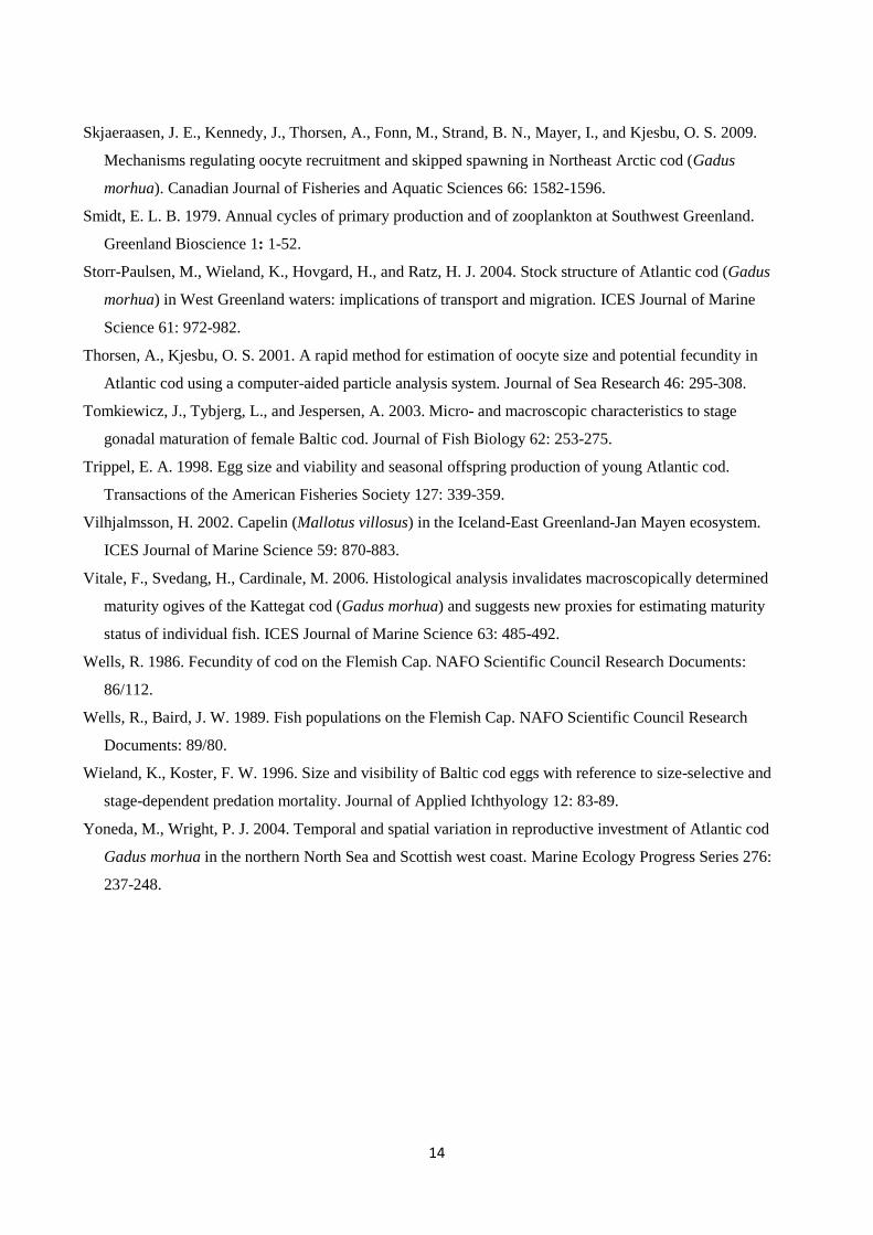
14
Skjaeraasen, J. E., Kennedy, J., Thorsen, A., Fonn, M., Strand, B. N., Mayer, I., and Kjesbu, O. S. 2009.
Mechanisms regulating oocyte recruitment and skipped spawning in Northeast Arctic cod (Gadus
morhua). Canadian Journal of Fisheries and Aquatic Sciences 66: 1582-1596.
Smidt, E. L. B. 1979. Annual cycles of primary production and of zooplankton at Southwest Greenland.
Greenland Bioscience 1: 1-52.
Storr-Paulsen, M., Wieland, K., Hovgard, H., and Ratz, H. J. 2004. Stock structure of Atlantic cod (Gadus
morhua) in West Greenland waters: implications of transport and migration. ICES Journal of Marine
Science 61: 972-982.
Thorsen, A., Kjesbu, O. S. 2001. A rapid method for estimation of oocyte size and potential fecundity in
Atlantic cod using a computer-aided particle analysis system. Journal of Sea Research 46: 295-308.
Tomkiewicz, J., Tybjerg, L., and Jespersen, A. 2003. Micro- and macroscopic characteristics to stage
gonadal maturation of female Baltic cod. Journal of Fish Biology 62: 253-275.
Trippel, E. A. 1998. Egg size and viability and seasonal offspring production of young Atlantic cod.
Transactions of the American Fisheries Society 127: 339-359.
Vilhjalmsson, H. 2002. Capelin (Mallotus villosus) in the Iceland-East Greenland-Jan Mayen ecosystem.
ICES Journal of Marine Science 59: 870-883.
Vitale, F., Svedang, H., Cardinale, M. 2006. Histological analysis invalidates macroscopically determined
maturity ogives of the Kattegat cod (Gadus morhua) and suggests new proxies for estimating maturity
status of individual fish. ICES Journal of Marine Science 63: 485-492.
Wells, R. 1986. Fecundity of cod on the Flemish Cap. NAFO Scientific Council Research Documents:
86/112.
Wells, R., Baird, J. W. 1989. Fish populations on the Flemish Cap. NAFO Scientific Council Research
Documents: 89/80.
Wieland, K., Koster, F. W. 1996. Size and visibility of Baltic cod eggs with reference to size-selective and
stage-dependent predation mortality. Journal of Applied Ichthyology 12: 83-89.
Yoneda, M., Wright, P. J. 2004. Temporal and spatial variation in reproductive investment of Atlantic cod
Gadus morhua in the northern North Sea and Scottish west coast. Marine Ecology Progress Series 276:
237-248.

15
Table 1
Mean potential fecundity (no. eggs 106) of female Atlantic cod from various populations. When an
empirical relationship was used to calculate the potential fecundity, the midpoint of each length group is
used. The mean fecundity is based on an un-weighted average of the individual groups. In Canadian waters
several references are listed, but only minimum and maximum fecundity are reported. F=potential fecundity,
LT=total length.
Length groups (cm)
]40-45] ]45-50] ]50-55] ]55-60] ]60-65] ]65-70] ]70-75] Mean
West Greenland (N) 0.236 (8) 0.340 (9) 0.523 (11) 0.896 (12) 0.986 (7) 0.945 (3) 1.409 (2) 0.762 (52)
Barents Seaa 0.221 0.318 0.442 0.599 0.791 1.024 1.304 0.671
Icelandb 0.155 0.253 0.391 0.582 0.838 1.17 1.604 0.714
North seac 0.428 0.648 0.941 1.322 1.804 2.403 3.137 1.526
Balticd 0.769 1.046 1.426 1.860 2.373 2.971 3.660 2.018
Canadae 0.112-0.468 0.172-0.613 0.253-0.781 0.355-0.974 0.470-1.191 0.609-1.435 0.775-1.706 0.392-1.024
a Kjesbu et al. (1998). Based on averaged empirical relationships in five years from 1986-1991: F=8.0-7 LT3,3279.
b Marteinsdottir and Begg (2002): F=0.0118 LT4.372
c Yoneda and Wright (2004): The relationship for inshore North Sea cod (INS) is used: F=0.361 LT3.73
d Kraus et al. (2000). The relationship covering all sampled months is used: F=13.53 LT2.92
e Various areas considered:
Pinhorn (1984): Placentia Bay: F=53.703 LT2.42
Pinhorn (1984): St. Pierre Bank: F=0.417 LT3,37
Wells (1986) and Wells and Baird (1989): Flemish cap: F=1.172 LT3,16
May (1967): Southern Grand Bank (NAFO area 3N): F=0.089 LT3,81
May (1967): Southern Grand Bank (NAFO area 3O): F=0.054 LT3.88
Buzeta and Wainwood (1982): Southern Gulf of St. Lawrence: F=1.1 LT3.28

16
Fig. 1
The study area on the Greenlandic west coast. All sampled stations are marked. White circles indicate
stations classified as being in the inner region of the fjord. Filled circles indicate stations classified as being
in the outer region of the fjord. Numbers indicate the sample size at the individual stations
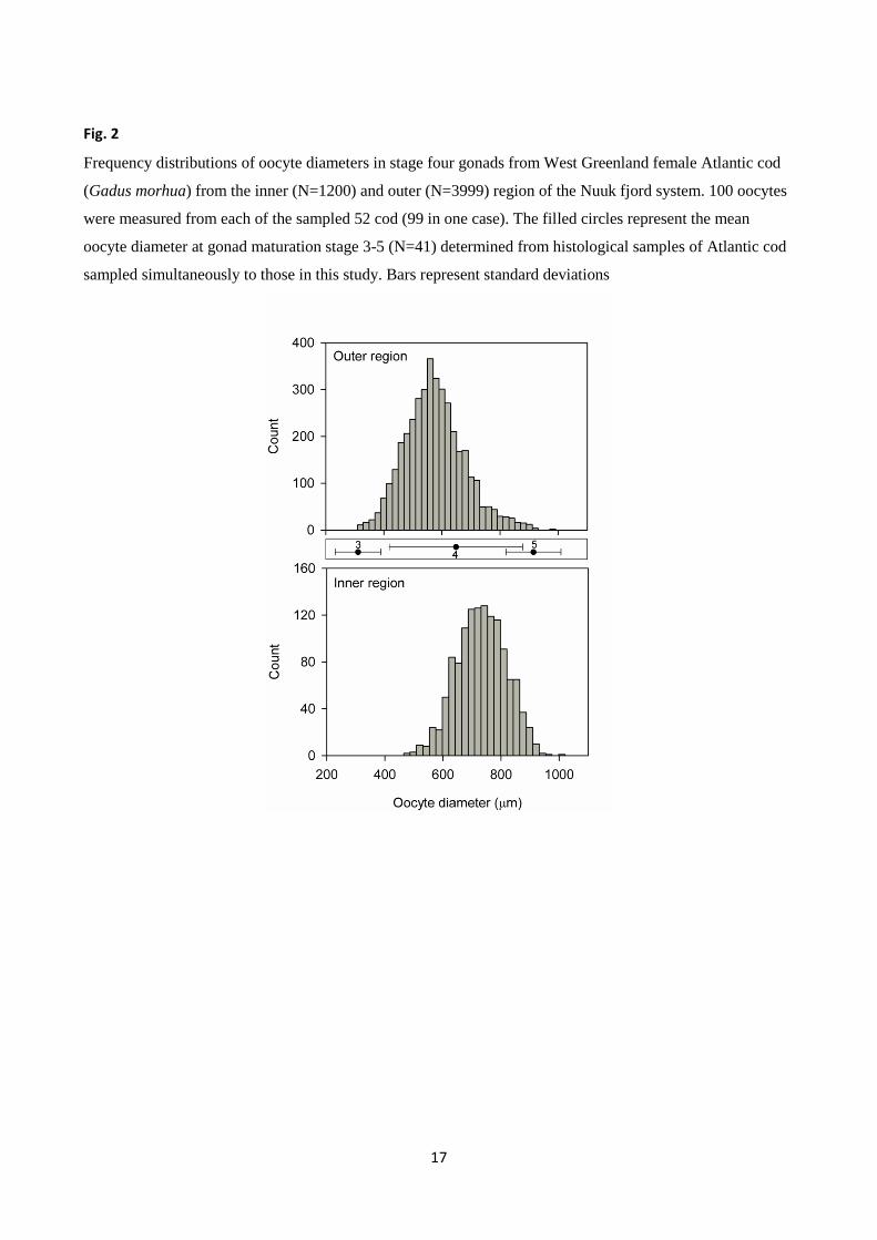
17
Fig. 2
Frequency distributions of oocyte diameters in stage four gonads from West Greenland female Atlantic cod
(Gadus morhua) from the inner (N=1200) and outer (N=3999) region of the Nuuk fjord system. 100 oocytes
were measured from each of the sampled 52 cod (99 in one case). The filled circles represent the mean
oocyte diameter at gonad maturation stage 3-5 (N=41) determined from histological samples of Atlantic cod
sampled simultaneously to those in this study. Bars represent standard deviations

18
Fig. 3
Redone from Thorsen and Kjesbu (2001). The line represents the relationship between mean oocyte diameter
(μm) and oocyty density (no. eggs g-1
) as determined for Northeast arctic cod by Thorsen and Kjesbu (2001):
Oocyte density = 2.137 1011 oocyte diameter
-2.700. The filled dots shows the results from a 1 g manually
counted sub sample using fish from this study and the corresponding mean oocyte diameter as determined
using the auto-diametric analysis (see materials and methods)

19
Fig. 4
The mean potential fecundity (no. eggs 106) in West Greenland female Atlantic cod (Gadus morhua) from
the Nuuk fjord system. Open circles: cod from the inner region of the fjord (N=12). Filled circles: cod from
the outer region of the fjord (N=40). Lines represents linear regression done separately for each area on the
full data set (lines are coincident): Inner region, Y = 0.1068 + 0.1184x, r2 = 0.69, P=0.021. Outer region, y =
0.1079 + 0.1189 x, r2=0.72, P<0.0001, where the length groups are numbered sequentially from 1-9. Bars
represent standard error.

20
Fig. 5
The mean egg energy content (J) in female Atlantic cod (Gadus morhua) sampled in the inner (open circles,
N=13) and outer (filled circles, N=39) region of the Nuuk fjord system as a function of gutted weight (g).
Bars indicate standard error

21
Fig. 6
a: total gonad energy content (J) of West Greenland female inshore cod (Gadus morhua) from the Nuuk fjord
as a function of total cod somatic calorific value (J). Open circles: inner region of the Nuuk fjord. Filled
circles: outer region of the Nuuk fjord. Lines represent linear regression and dotted lines are 95% confidence
intervals. Y = 0.28510x -520 and Y = 0.1336x -236 for the inner (P=0.0002) and outer (P<0.0001) region
respectively.
b: Total energy content of female gonads relative to total cod somatic energy content (%) as a function of
female cod size in terms of energy (J). Based on linear regressions from Figure 6a

Paper VI
An Ecopath model for the Nuuk fjord, Greenland
R. Hedeholm
Unfinished manuscript
1
An Ecopath model for the Nuuk fjord, Greenland
1, 2Hedeholm R.
1Marine Ecology, Department of Biological Sciences, Aarhus University. Building 1135, Ole Worms allé 1,
8000 Århus C, Denmark
2 Greenland Climate Research Centre, c/o Greenland Institute of Natural Resources, PO Box 570, 3900
Nuuk, Greenland
*Author to whom correspondence should be addressed. Tel.: +45 8942 4392; fax: +45 8942 4387; email:
Abstract
Capelin (Mallotus villosus) and Atlantic cod (Gadus morhua) are the dominant fish species in many sub-
arctic ecosystems. This is also the case in the lightly exploited Nuuk fjord, West Greenland (64˚N), but the
future may include an intensified fishery on both species with subsequent ecosystem changes as a result.
Here, a mass-balanced 19 compartment Ecopath model is presented for the Nuuk fjord, aiming to describe
system energy flow and determine the relative importance of its key species. Additionally, three Ecosim
scenarios are presented to explore the ecosystem response to different capelin fishing intensities (Low:
1.32 g C m-2 yr-1; Medium: 4.37 g C m-2 yr-1; High: 5.29 g C m-2 yr-1). The system was dominated by high
primary producer and capelin biomasses (7.0 g C m-2 yr-1 and 7.3 g C m-2 yr-1, respectively). Capelin in turn
constituted the main prey of higher trophic levels and was an intermediate energy node. Consistent with
this, primary producers and capelin were estimated as the most important groups through trophic impact
and keystoneness analysis. Total system catches were restricted to high trophic levels (mean=3.8) and
required 17.5% of the primary production with zooplankton (30%) and large capelin (22%) having the
highest demands. The low capelin fishing intensity scenario resulted in little system impact, but with
increasing intensity noticeable declines were seen in both capelin and cod with other groups benefitting
from reduced competition. Accordingly, a future fishery should be based on further knowledge on capelin
stock structure and its trophic position in relation to top predators.
2
Introduction
The Nuuk fjord is a sub-arctic fjord system on the Greenlandic West coast covering approximately 2000
km2. The key fish species in the system are capelin (Mallotus villosus) and Atlantic cod (Gadus morhua)
which both spawn within the fjord (Smidt, 1979; Friis-Rødel and Kanneworff, 2002). Both species are
present throughout Greenland, but supposedly have local genetically distinct populations in the Nuuk fjord
(Sørensen and Simonsen, 1988; Storr-Paulsen et al., 2004) which renders them vulnerable to over-
exploitation on a local scale. The Nuuk fjord system is commercially lightly exploited and of fishes, only cod
are fished beyond that of local use, but in limited amounts (2009 tonnes caught in 2009, Anonymous,
2010). However, there have been several trial fisheries for capelin in the region, and currently the cod
fishery is not limited by quotas but rather by low prices, suggesting a more intense fishery if prices increase.
The Nuuk fjord system has the characteristics of a wasp-waist system. This entails that capelin inhabits an
intermediate trophic level and is the primary mediator of energy from lower to higher trophic levels (Cury
et al., 2000). Due to this key position in the ecosystem, variability in capelin biomass (of natural or
anthropogenic origin) can have ecosystem impacts from both a top-down and bottom-up perspective
(Arrhenius and Hansson, 1993; Vilhjalmsson, 2002). Similarly, the cascading effects of a changed cod
biomass have been documented in several occasions often as a result of a population collapse following
overexploitation (Frank et al., 2005).
This study aims to describe the ecological interactions and carbon flow of the Nuuk fjord system in a lightly
exploited state. This serves as a first attempt to join and quantify knowledge from the area and will provide
insight into the importance of capelin and cod to energy flow. Such knowledge is essential for future local
management on these species if they are to be fished. Additionally, studies on capelin life history traits
from the region suggests a large effect of climatic changes and if such effects are to be put into an
ecosystem context a more holistic approach is needed. Hence, the carbon flow of the Nuuk fjord system is
quantified using the Ecopath mass balance model concept (Polovina, 1984; Christensen and Walters, 2004).
This is done with special emphasis on key species capelin and cod and using the Ecosim component of the
Ecopath software a future capelin fishery is modelled and its effects on the ecosystem are described.
Materials and Methods
Study site
The Nuuk fjord is located on the Greenlandic west coast (64˚18N, 51˚11W, Fig 1). The fjord has an average
depth of approximately 300 m with a sill at the fjord entrance of 250 m. The tidal amplitude is 4 m ensuring
a large vertical mixing. Glaciers in the inner fjord introduce a large summer run off which stabilizes the
water column in early spring. Average temperature within the fjord is approximately 2˚C, with surface

3
waters reaching 4˚C in the summer months while bottom water stays between 1-1.5˚C. Primary production
peaks in July coincident with the highest PAR radiance (Jensen and Rasch, 2008, Mikkelsen et al. in prep.).
For a more detailed description on fjord hydrography see Jensen and Rasch (2008).
The Ecopath model
The mass balance model was based on the Ecopath with Ecosim version 6.0 software (Christensen et al.,
2005; http://ecopath.org). Ecopath creates a mass balanced static snapshot of the ecosystem using two
master equations. This is under the assumption that the production of a group (species or guild) equals the
biomass lost to fishing, export, predation and natural mortality. This is formally expressed as:
Pi = Yi + BiM2i + Ei + Pi(1 − EEi) + BAi
where Pi is the production of the ecological group i, which equals sum of catches (Yi), predated biomass
(BiM2i), net migration (Ei), other mortalities (M0i, disease, old age) and biomass accumulation (BAi) (Pauly et
al., 2000). MOi is given by M0i = Pi(1−EEi), where the ecotrophic efficiency (EEi) is the fraction of the
production of a group that is accounted for in the models, through predation, fishing and other export, or
biomass accumulation. In addition to this overall mass-balance equation each individual group in the model
is balanced according to: Consumption = Production + Respiration + Unassimilated food.
In addition to these basic data, the diet composition of all groups must also be entered. This is done by
dividing the average yearly prey intake into the other system groups according to the share made up by
each group.
Input data
All data is entered as gram carbon m-2 year-1 (g C m-2 yr-1) and conversion factors from other units can be
seen in appendix A. The Nuuk fjord is represented by 19 ecological groups most of which are comprised of
more than one ecologically similar species (Table 1). Additional groups could easily be implemented (e.g.
bacteria and birds), but as this is the first attempt to model the area and data on some groups is non-
existing, the model should to some extent be considered a minimal realistic model. However, one focus of
the study was to increase understanding of the pelagic interdependencies and accordingly, pelagic species
were represented with finer resolution than the benthic community. Hence, the benthic community was
jointly grouped as “benthos” and due to this grouping not all included species are mentioned (Table I) but
see Sejr et al. (2010) for a more complete species list. Although ecologically important, birds and bacteria
were left out of the model as only little uncertain data are available. This may affect the model result on
some levels (see discussion), but previous versions of the model that included these groups yielded models
that did could not be reasonably balanced or produced unlikely results. Also, macro algae, Greenland

4
sharks (Somniosus microcephalus) and certain fish species (i.e. lumpsucker (Cyclopterus lumpus)) are not
included in the model. For the latter two no biomass estimates or other data exists locally (or globally) and
for the former their habitat makes up an insignificant amount of the fjord. All input data are summarized in
Table I and the estimated diet composition of all groups in Table II.
Data from the Nuuk fjord were used when possible and otherwise personal communications with local
experts or literature values from similar sub-arctic systems were applied. Especially data from Disko Bay
(69˚N) has been used as it is on the same coast line and represents a similar ecosystem. Additionally, the
model for Sørfjord in Northern Norway by Pedersen et al. (2008) was consulted as this model represents a
lightly exploited cod dominated system similar to the system addressed here. Whenever possible, the
model represents the Nuuk fjord 2007 or 2008 situation to reduce inter-year variability.
For all groups the following parameters are needed to balance the model: Yi, Bi, P/Bi, Q/Bi, EEi and DCji.
Besides catches (Yi) and complete diet (DCji) one out of the remaining parameters can be left out as
program algorithms will estimate it based on the other parameters (Christensen et al., 2005). Under
steady-state conditions the P/Bi parameter is equal to total mortality, Z (Allen, 1971), which was used in
estimating P/Bi for cod.
Some model groups were defined as “ecological anchors” and served as fixed holding points in the model
balancing process and were only changed when other options did not seem reasonable. These anchors
were groups where good quality local data were available and included primary producers, cod, capelin,
zooplankton and detritus and to lesser extent biomass estimates on whales, fishes, shrimp and other large
zooplankton groups (see appendix A). Only cod and seals are caught commercially in the system and catch
data were available for these species. All other catches are limited to that of local hunters and was
considered insignificant for the model, although its extent is unknown.
Model balancing was done by focusing on the most severe problems rather than employing a top-down or
bottom-up approach and was generally based on suggestions in Christensen et al. (2005). Hence, initially
the ecotrophic efficiency (EEi) values for the individual groups were evaluated and adjusted to fit within the
0-1 range. When these were balanced the remaining output parameters were checked (especially the
growth efficiency, P/Q) and if outside a reasonable ecological range the model was modified. Diet was used
as the initial balancing parameter as diet composition data is scarce for the Nuuk fjord and often represents
a temporal limited snapshot of the integrated feeding behaviour. If changes here were too drastic
compared to the original data or other studies other parameter changes were made; most often group
biomass (Table III).
5
Ecosim input
The Ecosim component allows for time based dynamic simulations of changing fishing intensity on the
ecosystem. It uses input from the Ecopath model and based on a set of linear and differential equations
derived from the Ecopath master equation it calculates future biomasses of all groups based on a pre-set
fishing scenario (Christensen et al., 2005). The master equation of Ecosim is:
𝑑𝐵𝑖
𝑑𝑡= 𝑔𝑖 ∑𝑖𝑄𝑗𝑖 − ∑𝑖𝑄𝑖𝑗 + 𝐼𝑖 − 𝑀𝑂𝑖 + 𝐹𝑖 + 𝑒𝑖 ∗ 𝐵𝑖
where dBi/dt represents the growth rate of group i during the time interval dt in terms of its biomass Bi, gi is
the net growth efficiency (production/consumption ratio), MOi is the non-predation natural mortality rate,
Fi is fishing mortality rate, ei is emigration rate, Ii is immigration rate. The key parameter, consumption rates
Qji, are calculated based on the “foraging arena” concept, where Bi’s are divided into vulnerable and
invulnerable components, and it is the transfer rate between these two parameters that determines if
control is driven by top-down (i.e. Lotka–Volterra), bottom-up (i.e. donor-driven) or of an intermediate type
(Walters et al., 1997). If vulnerabilities are low an increase in predator abundance causes little change in
prey abundance and vice versa. The vulnerabilities for all predator-prey interactions are pre-set prior to
Ecosim model runs, and model performance is highly dependent on vulnerability settings. Time series data
on abundances and fishing intensities are advisable to use in obtaining the best estimates of vulnerabilities.
This is done by adjusting vulnerabilities in order to achieve congruence between observed and modelled
abundances under known conditions (e.g. Griffiths et al., 2010). However, no time series data are available
for the Nuuk fjord except for cod catches and such calibration procedures were not possible. Hence, all
vulnerabilities were set at default values (2.0) in the model assuming neither top-down or bottom-up
control.
Based on the Icelandic capelin fishery in the 1990’s and coincident biomass estimates of the capelin stock
(Vilhjalmsson and Carscadden, 2002) three Ecosim scenarios were set up. Current catches (e.g. cod and
seals) were kept constant and only the fishing intensity on large capelin was modified. The scenarios were
1) a fishing pressure relatively identical to the Icelandic (67% of the fishable population caught – 4.37 g C m-
2 yr-1), 2) a low fishing pressure (20% - 1.32 g C m-2 yr-1) and 3) intense (over)fishing pressure (80% - 5.29 g C
m-2 yr-1). Each scenario was allowed to run for ten years with fixed fishing intensities. For the three
scenarios the relative biomass changes for cod and capelin groups as well as groups being the most
affected (>50% change in biomass) are reported on graphically.

6
Model output
Summary statistics
The system is described in a number of summary statistics. In addition to the estimated missing ecosystem
parameters (typically EEi) I have chosen the ones most relevant in evaluating the questions posed in this
study, as well as those describing the system in general.
The total system throughput represents the sum of all flows in the ecosystem and is useful in system
comparisons representing flows from all consumption, respiration, export and flow to the detritus. The
maturity of the system was evaluated by the ratio between system primary production and respiration with
values around one indicating a mature system, values >1 indicating a young system and values <1 typical of
heavily polluted systems (Odum, 1971). A further overall description of the system is presented through
transfer efficiencies (%). This is the proportion of energy transferred between trophic levels and is
calculated as the ratio between the export at a trophic level plus the transferred flow to the next trophic
level and the total throughput on that trophic level. Furthermore, fractional trophic levels were estimated
for all groups with producers having trophic level one and all other group trophic levels were equivalent to
the weighted average of the consumed prey’s trophic level.
Keystoneness and mixed trophic impact
To evaluate each individual group as a potential key species in the ecosystem a keystoneness index was
calculated using the Ecopath routine. The routine assigns a value to each group based on its impact on
other groups in relation to its own biomass. The index combines a measure of group biomass in relation to
total system biomass and the mixed trophic impact which calculates the impact a change in specific group
biomass has on other groups. Hence, a group with a relatively small biomass having a large ecosystem
impact gets a high value (Libralato et al., 2006). The mixed trophic impact also allows gives a graphical
representation of how changes in different groups quantitatively affect other groups, positively or
negatively. Adding to this is a flow diagram of the system, where each group is represented with relative
biomasses and all interactions are scaled to strength. As the detritus biomass was relatively large in the
model this group has been assigned a biomass value of 0.1 in this context to allow for distinction between
other groups.

7
Results
Model balancing
The initial model had high EE values for especially krill, amphipods and mesozooplankton. However, simply
increasing the biomass (i.e. a bottom-up approach) of these groups would lead to unrealistic estimates.
Rather, the high EE values were a result of intense capelin predation pressure caused by the combination of
a high biomass of capelin and a diet consisting of few prey groups. Capelin data on biomass was considered
an “ecological anchor” and was not changed (Appendix A). This left capelin diet information as balancing
parameter but this was also based on local information and only slight changes were made to the diet
composition. Instead, the diet import was increased from 0.5 to 0.9 (for both small and large capelin). This
did not completely balance the model for krill but krill biomass was based on one sampling transect in May
2007 and based on Pedersen et al. (2008) krill biomass was increased to 1.5 (from 0.34) to accommodate
predatory demands. Similarly, the biomass of amphipods was increased (Table II).
EE for phytoplankton was initially too high and biomass was increased slightly for the group in spite of it
being considered an “ecological anchor”. However, calculations of biomass was based on integrated
chlorophyll values, and the depth (0-150 m) may have been set too low to include all production and
increasing biomass was the only approach that allowed for realistic model estimates (see discussion).
The estimated Von Bertalannfy growth parameter “k” for cod was low (0.069), even though cod growth is
slow in the area (Brander, 1995). Using catch data from the region the growth equation was slightly
modified (Winf and Wmat) and “k” was re-estimated (0.091).
Other model estimates that caused an imbalance in either EE or other parameters such as gross food
conversion (GE, production/consumption) where balanced by changing diet compositions for various
groups. These included only minor changes and I refer to Table II for an overview of the changes made.
Model output – group level
Phytoplankton production was 125 g C m-2 yr-1 and of this 117 g C m-2 yr-1 is directly consumed by especially
zooplankton and krill. Accordingly, the zooplankton groups had the highest flow to detritus (41 g C m-2 yr-1
combined for proto- and mesozooplankton) followed by phytoplankton (8 g C m-2 yr-1). The detritus group
was predated upon primarily by the benthos group (24 g C m-2 yr-1) but detritus EE remained low (0.38) but
this would increase if a bacteria group was included in the model. EE for whales was 0.0 as they accumulate
biomass export it through migration and the same is partly true for seals, albeit hunting removes some
biomass (0.003 g C m-2 yr-1) giving an EE of 0.49. The only other group subject to fishing is large cod, but EE
remains low for the group (0.43). EE for the small cod was only 0.05 similar to that of small capelin which

8
were the lowest EE values except for whales. Large capelin had an EE of 0.53 whereas the other small
pelagics had a higher value of 0.94.
Large pelagics had the highest trophic level (4.07, Table III) with large cod (3.85), seals (3.83) and large
benthic fish (3.66) almost equally high. Large capelin had a trophic level of 2.96 and there was a large gap
to lower levels such as mesozooplankton (2.16) and krill (2.15).
Mixed trophic impact and keystoneness
The mixed trophic impact quantifies the effect perturbations in a group biomass will have on other groups
(Fig. 2). Phytoplankton, and to some extent other lower trophic levels, fuels the ecosystem and had
pronounced positive impacts on higher trophic levels. Many groups had little impact as a result of a
relatively low biomass (e.g. small pelagics). Capelin are in comparison very abundant and this is also
reflected in negative impacts on prey groups and positive impacts on predators such as cod. Such direct
positive/negative interactions between predator-prey connections suggest an interactive system that is
susceptible to perturbations. For instance, an increase in large capelin biomass negatively affects prey but
also small pelagics as a result of prey competition. All groups had negative impacts on themselves as a
result of intra-group competition.
The patterns from the mixed trophic impact were also evident in the keystoneness analysis (Fig. 3). Hence,
the most important group were phytoplankton followed by large capelin. This was followed by
mesozooplankton and amphipods while large cod is only number eleven in keystoneness ranking. This was
most likely caused by the high trophic level of cod and the relatively large dependence on a single prey item
(capelin). The keystoneness index is negatively related to biomass (Libralato et al., 2006), which emphasizes
the high ranking of capelin and phytoplankton as their biomass is only surpassed by the benthos group. It is
however noticeable that no groups have values above one indicating that no one group has a clear defining
structuring role in the system.
Model output - community level
Summary statistics on the system are given in Table IV and the relative flows in Fig. 4. The system transfer
efficiency (9.3%) is the geometric mean of all trophic levels and a more detailed description can be seen in
Table V with efficiency being similar between detritus and primary producers. Consumption of top predator
seals required 19% of primary production while zooplankton groups (30%) and large capelin (22%) had the
highest single group requirements. Although low in absolute terms (0.06 g C m-2 yr-1) total catches in the
system required 17.5% of the primary production as they were limited to high trophic level species (seals
and large cod, mean trophic level=3.8).

9
The total primary production/total respiration ratio was 0.94 and the connectance index was 0.27 (Table
IV). The later is the realized links in the system in relation to the total possible number of links. These two
parameters are linked as both gives an indication of ecosystem maturity as does the omnivory index which
was 0.25, describing the degree of consumer specialization (0=specialist).
Ecosim scenarios
All scenarios had a large impact on certain group biomasses. The scenario equalling the Icelandic fishing
intensity (4.37 g C m-2 yr-1, Fig. 5 middle) while at the same time maintaining other fishing intensities (large
cod and seal) caused a decline in all cod and capelin groups with biomasses being reduced below half of
current estimates. Biomass increases were seen in small pelagics and large benthic fish which doubled; a
trend consistent in all scenarios. With low capelin fishing intensity, large capelin biomass increased slightly
while small capelin decreased (Fig. 5 top). Cod biomass decreased initially but seemed to rebound to initial
levels at the end of the period as did the biomass of large capelin. The decrease in small capelin biomass
was seen in all scenarios and is also evident when removing all fishing (not shown). Otherwise, the no-
fishing scenario generally caused little changes in any groups. However, large capelin biomass increased
and coincidently with the large capelin increase, the cod groups increased slightly. The scenario with high
fishing intensity on large capelin (5.29 g c m-2 yr-1) was detrimental to all cod and capelin groups with all
biomasses decreasing to approximately 25% of initial estimates (Fig. 5 bottom). Benefitting from this was
small pelagics with a tripled biomass.
Discussion
Parameterization and group level
The estimated parameters and subsequent model balancing only represents one possible interpretation of
the data, and the model can only give as good a fit as the quality of the input data allows (Essington, 2007).
However, the model does provide insight into the system, joins current knowledge and identifies areas
where further data is needed to improve the model. These areas especially include high trophic level fish
groups and other high levels. Hence, the “ecological anchors”, defined as high quality data in certain
groups, were mostly limited to lower trophic levels with data on phytoplankton, zooplankton and capelin
being the best in the model followed partly by cod. To generally improve the model, studies on ecosystem
interactions such as trophic levels (e.g. isotopic analyses, Fredriksen, 2003) would allow for better
estimates of model fit. Furthermore, specific studies on feeding and abundance on especially higher trophic
levels would ensure better model estimates in specific groups. This also includes groups excluded from the
present model, such as birds, bacteria and certain species of mammals and the grouping of benthos needs
10
better resolution (Pedersen et al., 2008). In spite of these shortcomings, the model was fairly easily
balanced and estimates are within reasonable ranges and certain patterns can be deduced, especially on
mid- and lower trophic levels.
Phytoplankton EE was very high for the system (0.93) also in comparison with other sub-arctic systems (e.g.
Northern Norway, Pedersen et al. 2008, EE=0.80; Barents Sea, Blanchard et al., 2002, EE=0.29) and
phytoplankton biomass was increased from the initial model due to too high EE value. This suggests a very
effective grazing community in the system, which may also be partly true. However, phytoplankton
biomass may also have been underestimated as data for this parameter are collected at a part of the fjord
where the vertical mixing is very pronounced (Jensen and Rasch, 2008; J. Mortensen, pres. comm.). Here,
the chlorophyll measurements where integrated to a depth of 150 meters, but this should perhaps be
increased (200-250 m) thus increasing biomass and production and subsequently lowering the EE value. In
general, a deficit of available resources at lower trophic levels was a problem in the initial model and the
biomasses of zooplankton groups were increased but EE values are still high for these groups (Table III). The
initial reason for this large demand was caused by intense capelin predation. Capelin is by far the most
abundant living group in the system, and the biomass and diet estimate are among the best model
estimates (Appendix A). Hence, these were kept unchanged and the only option that allowed for model
balancing was increasing capelin diet import to 90% (changing other proportions relatively) as system
productivity would otherwise be to low irrespective of balancing approach. Hence, the migration pattern of
Greenlandic capelin reviewed by Friis-Rødel and Kanneworff (2002) is supported in this study with almost
all consumption taking place outside the fjord, but nevertheless predation in the fjord is so intense that
zooplankton groups EE remain high (Table III). This apparent key role of capelin with the capabilities of
exerting top-down control was also supported by the mixed trophic impact and keystoneness analyses
where capelin was the second most important group underlining its importance as both predator and prey.
Hence, capelin appears to play a key role in the system consistent with the wasp-waist ecosystem theory
(Bakun, 2006) but due to the large capelin biomass, bottom-up control does not appear to be as
pronounced, which makes the system less susceptible to capelin inter-year variation. Such system
redundancy maintained by high wasp-waist species abundance is also a typical wasp-waist system
characteristic (Jarre, 2003). This is also reflected in the relatively low EE for large capelin (0.52) compared to
other Ecopath models (e.g. 0.79, Blanchard et al., 2002) and the much higher EE value of other small
pelagics (EE=0.94). However, this may also partly be an artefact of capelin consumption being
underestimated in the model. Hence, during capelin off shore migration they are a primary prey of minke
whales (Balaenoptera acutorostrata) and harbour porpoise (Phocoena phocoena) which are common in the
off shore region (Neve, 2000; Bergstrøm and Vilhjálmsson, 2006) as well as other species of seals (Ringed
11
seals (Phoca hispida), Hooded seals (Cystophora cristata) not included in the model. Furthermore, bird
predators are not included and these could consume a noticeable amount of capelin (Merkel et al., 2002),
although this is more likely primarily small capelin which also could explain the extremely low EE values for
this group (0.05).
No data on historic capelin abundance exists, but a contributing factor in maintaining the current apparent
high capelin abundance could be coincident low cod population size. Greenlandic waters have historically
supported large cod populations evidenced by a large fishery (Horsted, 2000) and prey composition data
(Table II) suggests that this will have had an impact on capelin through an intense predation pressure.
Indeed, the importance of capelin to cod is found in many waters (Pálsson, 1997; Nielsen and Andersen,
2001) and correlations between capelin abundance and cod condition have been suggested (Rose and
O'Driscoll, 2002; Hedeholm et al. Unpublished manuscript). Cod is presently the only commercially
exploited fish species in the system and it had an estimated trophic level of 3.85 which is similar to other
systems (range 3.7-4.4) albeit slightly lower (see studies reviewed by Pedersen et al., 2008). The biomass of
large cod (0.21) is high compared to heavily fished areas such as the North sea (B=0.07, Christensen, 1995)
and similar to lightly exploited systems such as the Sørfjord, Norway (B=0.22, Pedersen et al., 2008). Based
on published Ecopath models, Tudela et al. (2005) categorized ecosystems as either over- or not exploited
using the trophic level of the catch and the primary production required to support it. The values estimated
here (Catch trophic level=3.8, Primary production required=17.5%) qualifies the Nuuk fjord ecosystem as
belonging to the sustainably fished ecosystems, which is consisted with the relatively species poor and
limited catch. Hence, current fisheries do not appear to be detrimental to the cod population.
Community level
The total system throughput was 545 g C m-2 yr-1 (Table IV). This is very close to other sub-arctic systems
(Blanchard et al., 2002; Pedersen et al., 2008) indicating that the current model is accurate as well as
suggesting some shared characteristics of the systems.
The transfer efficiencies declined with increasing trophic level (Table V) which is agreement with that of
theoretical ecology (Odum, 1971). The mean of the individual transfer efficiencies was 9.8% and this is in
good agreement with a value of 10% suggested for other marine ecosystems (Pauly and Christensen, 1995)
but lower (half) than estimates from other high latitude systems (Bowering and Lilly, 1992; Pedersen et al.,
2008) which are often efficient short food chains (Richardson, 2008). The reason for this is probably a much
lower fishing intensity in the Nuuk fjord compared to other systems, and especially a fishery at lower
trophic levels would increase the transfer efficiency. Hence, in the Nuuk fjord the primary production
required to support total system catches was 17.5% compared to 65.5% in the Sørfjord model in northern

12
Norway (Pedersen et al., 2008) although the trophic level of the catch was similar (3.5 and 3.8 in Sørfjord
and Nuuk, respectively). The low values also entail that a lot of dead organic material (mainly fecal pellets)
flows to detritus and is subsequently re-mineralized which could also support the fairly high primary
biomass and production in the system (e.g. Pedersen et al., 2008).
The total primary production/total respiration ratio was 0.94 indicating a fairly mature system (Odum,
1971) consistent with a system that has not seen large perturbations through commercial catches and
again parallels to the similar Sørfjord system are evident in similar ratios (1.022, Pedersen et al., 2008).
Other overall system descriptors, the system omnivory index (0.25) and connectance index (0.27) describe
the inner linkage ecosystem structure and are expected to increase with system maturity as more links are
formed. Hence, as values here are similar to values presented in studies with higher total primary
production/total respiration ratios (Blanchard et al., 2002; Duan et al., 2009) both indexes were expected
to be higher. However, model structure in this study can offer some explanation. Hence, some realized links
are probably missed through poor/missing local diet data and the grouping will also have joint several links
into one link, most noticeably the benthos group, and this will reduce both connectance and omnivory
values.
Ecosim
In spite of the limitations imposed on the Ecosim simulations through lack of time series data and
subsequently more reliable vulnerability estimates and predator consumption rates, the general patterns in
the groups of most interest in this study (i.e. capelin and cod) seem valid and are based on good data.
Hence, the three Ecosim scenarios resulted in some general patterns suggesting the importance of capelin,
especially to cod. Hence, capelin biomass declined with increasing fishing intensity and this was coincident
with a negative response of cod groups (Fig. 5). This was also supported by the increase in cod biomass
coincident with that of capelin in the no-fishing scenario. Capelin prey groups krill and amphipods also
responded to capelin changes, increasing in abundance when capelin declined but less than 50%. The
zooplankton groups remained almost unchanged. In addition to these predator-prey responses underlining
capelin importance, the results indicate that the current inshore cod fishery is not negatively affecting the
cod population. However, if the current cod fishing intensity is kept constant with the introduction of a
capelin fishery the cod population will likely decline, and may have difficulties rebounding if capelin is
continuously fished (Rose and O'Driscoll, 2002). Such considerations are especially important as capelin
cohort strength can be expected to be highly variable (Vilhjalmsson, 2002), and if the management is not
accordingly flexible the potential for an overexploitation is eminent. This necessitates yearly surveys on the
stock size similar to those preformed routinely in Icelandic waters.

13
Small pelagics benefitted from the capelin fishery in all scenarios as a result of decreased prey competition
from capelin and reduced predation from small and large cod. This is in accordance with results from the
mixed trophic impact analysis, where an increase in capelin biomass caused a negative development in
small pelagics (Fig. 2). The large benthic fish was the last group to show any consistent change, increasing in
all scenarios. This was caused by little predation on the group, with only a small degree of cannibalism
(Table II). Had better data been available, groups such as seals and large cod would probably, to some
extent, feed on small stages of species in this group. Additionally, there is a local fishery on especially red
fish that has not been included in the study as the extent of the catches is unknown. Lastly, the catchability
of most species in this group is unknown and hence the biomass estimates are associated with uncertainty
and estimates are based on nearby coastal areas but if these are transferable to the fjord is unknown and
these results should not overly emphasized.
Small capelin declined in biomass initially in all scenarios and then stabilized at a low level. No ecological
explanation for this could be found and it is most likely a result of model parameterization. Hence, small
capelin biomass is estimated based on knowledge on large capelin, and the consistent decline could well be
a parameterization artefact and reflects the need to obtain further knowledge on small capelin in the
system. Alternatively, the response reflects incorrect vulnerabilities in the model. These should be re-
estimated but this is dependent in time series data on biomass and catches, and currently no monitoring
program on fish is available.
Conclusion
The present Ecopath model combines all present knowledge on the Nuuk fjord and demonstrates that
capelin is a key component of the Nuuk fjord ecosystem. It especially has the potential to top-down control
main prey groups due to a high biomass. It is also important as prey to many higher trophic levels, but clear
evidence of bottom-up control was not found. However, this may rest on the exclusion of certain important
ecological groups, and highlights the general need for more data on especially higher trophic levels. Ecosim
simulations suggest that a future fishery in capelin is possible, but must be managed from a multiple
species perspective as especially cod responds to capelin biomass variability.

14
References
Allen, K. R. 1971. Relation between Production and Biomass. Journal of the Fisheries Research Board of
Canada, 28(10): 1573-&.
Anonymous 2010. ICES North Western Working Group.
Arrhenius, F. and Hansson, S. 1993. Food-Consumption of Larval, Young and Adult Herring and Sprat in the
Baltic Sea. Marine Ecology-Progress Series, 96(2): 125-137.
Bakun, A. 2006. Wasp-waist populations and marine ecosystem dynamics: Navigating the "predator pit"
topographies. Progress in Oceanography, 68(2-4): 271-288.
Bergstrøm, B. and Vilhjálmsson, H. 2006. Cruise report and preliminary results of the Acoustic / pelagic
trawl survey off West Greenland for capelin and polar cod 2006, Greenland Institute of Natural
Resources: 60pp.
Blanchard, J. L., et al. 2002. Exploring marine mammal-fishery interactions using 'Ecopath with Ecosim':
modelling the Barents Sea ecosystem. Sci. Ser. Tech. Rep., CEFAS Lowestofy: 52pp.
Bowering, W. R. and Lilly, G. R. 1992. Greenland Halibut (Reinhardtius hippoglossoides) Off Southern
Labrador and Northeastern Newfoundland (Northwest Atlantic) Feed Primarily on Capelin
(Mallotus villosus). Netherlands Journal of Sea Research, 29(1-3): 211-222.
Brander, K. M. 1995. The effect of temperature on growth of Atlantic cod (Gadus morhua L.). ICES Journal
of Marine Science, 52: 1-10.
Christensen, V. 1995. A model of trophic interactions in the North Sea in 1981, the Year of the Stomach.
Dana, 11(1): 1-28.
Christensen, V. and Walters, C. J. 2004. Ecopath with Ecosim: methods, capabilities and limitations.
Ecological Modelling, 172(2-4): 109-139.
Christensen, V., et al. 2005. Ecopath with Ecosim: a User's guide.
Cury, P., et al. 2000. Small pelagics in upwelling systems: patterns of interaction and structural changes in
"wasp-waist" ecosystems. ICES Journal of Marine Science, 57(3): 603-618.
Duan, L. J., et al. 2009. Modeling changes in the coastal ecosystem of the Pearl River Estuary from 1981 to
1998. Ecological Modelling, 220(20): 2802-2818.
Essington, T. E. 2007. Evaluating the sensitivity of a trophic mass-balance model (Ecopath) to imprecise data
inputs. Canadian Journal of Fisheries and Aquatic Sciences, 64(4): 628-637.
Frank, K. T., et al. 2005. Trophic cascades in a formerly cod-dominated ecosystem. Science, 308(5728):
1621-1623.
Fredriksen, S. 2003. Food web studies in a Norwegian kelp forest based on stable isotope (delta C-13 and
delta N-15) analysis. Marine Ecology-Progress Series, 260: 71-81.

15
Friis-Rødel, E. and Kanneworff, P. 2002. A review of capelin (Mallotus villosus) in Greenland waters. ICES
Journal of Marine Science, 59(5): 890-896.
Griffiths, S. P., et al. 2010. Ecological effects of longline fishing and climate change on the pelagic ecosystem
off eastern Australia. Reviews in Fish Biology and Fisheries, 20(2): 239-272.
Horsted, S. A. 2000. A review of the cod fisheries at Greenland, 1910-1995. Journal of Northwest Atlantic
Fishery Science,(28): 1-109.
Jarre, A. 2003. Compiling the basis for assessment of responsible fisheries: forage fish off West Greenland.
Nuuk, Greenland Institute of Natural Resources: 48.
Jensen, L. M. and Rasch, M. 2008. Nuuk Ecological Reseach Operations. 1st Annual Report 2007., Nuuk
Ecological Research Operations: 112.
Libralato, S., et al. 2006. A method for identifying keystone species in food web models. Ecological
Modelling, 195(3-4): 153-171.
Merkel, F. R., et al. 2002. Winter seabird distribution and abundance off south-western Greenland, 1999.
Polar Research, 21(1): 17-36.
Neve, P. B. 2000. The diet of the minke whale in Greenland - A short review. Minke Whales, Harp and
Hooded Seals: Major Predators in the North Atlantic Ecosystem, 2: 92-96.
Nielsen, J. R. and Andersen, M. 2001. Feeding habits and density patterns of Greenland cod (Gadus ogac)
(Richardson 1836), at West Greenland compared to those of the coexisting Atlantic cod, Gadus
morhua L. Journal of Northwest Atlantic fishery science, 29: 1-22.
Odum, E. P. 1971. Fundamentals of Ecology. Philadelphia, W.B. Saunders Co.
Pálsson, Ó. K. 1997. Food and feeding of cod (Gadus morhua) Fjölstofnarannsóknir (Multispecies research)
1992-1995. J. Jakobsson and Ó. K. Pálsson. Reykjavik, Hafrannsóknastofnunin (Marine Research
Institute): 177-191.
Pauly, D. and Christensen, V. 1995. Primary Production Required to Sustain Global Fisheries. Nature,
374(6519): 255-257.
Pauly, D., et al. 2000. Ecopath, Ecosim, and Ecospace as tools for evaluating ecosystem impact of fisheries.
ICES Journal of Marine Science, 57(3): 697-706.
Pedersen, T., et al. 2008. Trophic model of a lightly exploited cod-dominated ecosystem. Ecological
Modelling, 214(2-4): 95-111.
Polovina, J. J. 1984. An overview of the ECOPATH model. Fishbyte, 2(2): 5-7.
Richardson, A. J. 2008. In hot water: zooplankton and climate change. ICES Journal of Marine Science, 65(3):
279-295.

16
Rose, G. A. and O'Driscoll, R. L. 2002. Capelin are good for cod: can the northern stock rebuild without
them? ICES Journal of Marine Science, 59(5): 1018-1026.
Sejr, M. K., et al. 2010. Macrobenthic species composition and diversity in the Godthaabsfjord system, SW
Greenland. Polar Biology, 33(4): 421-431.
Smidt, E. L. B. 1979. Annual cycles of primary production and of zooplankton at Southwest Greenland. .
Greenland Bioscience: 1-52.
Storr-Paulsen, M., et al. 2004. Stock structure of Atlantic cod (Gadus morhua) in West Greenland waters:
implications of transport and migration. ICES Journal of Marine Science, 61(6): 972-982.
Sørensen, E. F. and Simonsen, V. 1988. Genetic Differentiation among Populations of Capelin Mallotus
villosus from the West-Coast of Greenland. Journal of Applied Ichthyology-Zeitschrift Fur
Angewandte Ichthyologie, 4(1): 23-28.
Tudela, S., et al. 2005. Developing an operational reference framework for fisheries management on the
basis of a two-dimensional index of ecosystem impact. ICES Journal of Marine Science, 62(3): 585-
591.
Vilhjalmsson, H. 2002. Capelin (Mallotus villosus) in the Iceland-East Greenland-Jan Mayen ecosystem. ICES
Journal of Marine Science, 59(5): 870-883.
Vilhjalmsson, H. and Carscadden, J. E. 2002. Assessment surveys for capelin in the Iceland-East Greenland-
Jan Mayen area, 1978-2001. ICES Journal of Marine Science, 59(5): 1096-1104.
Walters, C., et al. 1997. Structuring dynamic models of exploited ecosystems from trophic mass-balance
assessments. Reviews in Fish Biology and Fisheries, 7(2): 139-172.

17
Table I
Individual groups and the main taxa included in the Ecopath model for the Nuuk Fjord system.
Group number Group name Taxa
1 Whales Megaptera novaeangliae 2 Seals Pagophilus groenlandica 3 Large benthic fish Anarhichas spp., Sebastes spp., Reinhardtius hippoglossoides, Boreogadus saida,
other fish (see Pedersen and Kanneworff (1995)) 4+5 Large and small cod Gadus morhua
6 Large pelagics Salmo salar, Salvelinus alpines, Melanogrammus aeglefinus, other fish (see Møller et al. (2010))
7 Small pelagics Myctophidae, Clupea harengus, Ammodytidae, juvenile stages of other fishes 8+9 Large and small capelin Mallotus villosus 10 Shrimps Pandalus borealis, Pandalus Montagui, Pandalus Propingus 11 Krill Thysanoessa raschii, Thysanoessa inermis, Thysanoessa longicaudata 12 Amphipods Parathemisto abyssorum, Parathemisto libulla 13 Scyphomedusae Siphonophora 14 Chaetognatha Sagitta elegans, Eukrohnia hamata 15 Mesozooplankton Calanus spp., Metridia spp., Pseudocalanus spp., Onacea spp., Microsetella spp. 16 Protozooplankton Heterotrophic dinoflagellates, ciliates 17 Phytoplanton 18 Benthos Crabs, echinoderms, clams, mussels, polychaetes, amphipods etc. 19 Detritus

18
Table II
Final diet inputs for the Nuuk fjord Ecopath model and the initial input in parentheses. Numbers represent the share of the diet (g C m-2 yr-1)
constituted by each group. All columns sum to one.
Predator/Prey 1 2 3 4 5 6 7 8 9 10 11 12 13 14 15 16 17 18
1: Whales
2: Seals
3: Large benthic fish
0.0729
4: Small cod 0.005 0.00506 0.0125
5: Large cod 0.005 0.000607
6: Large pelagics 0.010 (0.036)
7: Small pelagics 0.042 0.161 0.0842 0.100 (0.181)
0.040 (0.083)
0.01 (0.039)
8: Large capelin 0.104 0.155 (0.129)
0.0194 0.632 0.577 0.44 (0.40)
0.022 (0.0)
9: Small capelin 0.021 0.0194 0.104 0.033 (0.09)
0.17 (0.167)
10: Shrimps 0.010 0.0239 0.011 0.09
11: Krill 0.250 0.0617 0.195 0.011 0.028 0.009 0.29 (0.28)
0.0343 (0.171)
0.309 0.05 0.03
12: Amphipods 0.0017 0.155 0.053 0.01 0.307 0.29 (0.28)
0.02 (0.212)
0.10 0.0206 0.05
13: Scyphomedusae
0.05
14: Chaetognatha 0.025 0.0515 0.03 0.02
15: Meszooplankton
0.105 0.007 0.31 (0.30)
0.0234 (0.117)
0.02 (0.10)
0.55 (0.619)
0.50 (0.60)
0.75
16: Protozooplankton
0.10 0.08 (0.40)
0.28 0.14 0.069 (0.0)
0.27 (0.17)
0.20 0.15 0.05
17: Phytoplankton
0.20 0.71 0.75 0.90
18: Benthos 0.0017 0.244 0.105 0.150 (0.102)
0.002 0.32
19: Detritus 0.10 0.15 0.05 0.10 0.05 1.00
Import 0.583 0.750 0.900 (0.500)
0.900 (0.500)

19
Table III
Summary of basic in- and output for Nuuk fjord Ecopath model. Estimated parameters are shown in bold.
Parameter estimates from the balanced model is followed by the initial input/output. TL=Trophic level,
B=Biomass, P/B=Production/Biomass, C/B=Consumption/Biomass, EE=Ecotrophic Efficiency,
P/C=Production/Consumption, UA/C=Unassimilated/Consumption
Group name TL B P/B C/B EE P/C UA/C
1: Whales 3.53 (3.69) 0.0370 0.100 4.500 0.000 0.022 0.200 2: Seals 3.83 (4.34) 0.0595 0.102 17.410 0.494 (1.598) 0.006 0.200 3: Large benthic fish 3.66 (3.68) 0.0327 0.346 2.000 0.421 0.173 0.200 4: Small cod 3.92 (4.33) 0.1350 (0.0706) 1.500 (1.000) 5.368 (4.893) 0.051 (0.147) 0.279 (0.204) 0.200 5: Large cod 3.85 (4.32) 0,2080 0.683 1.875 0.432 0.364 0.200 6: Large pelagics 4.07 (4.36) 0.3000 0.100 1.436 0.345 (1.243) 0.070 0.200 7: Small pelagics 3.47 (3.50) 0.3000 0.500 (0.265) 2.000 0.938 (2.218) 0.250 (0.132) 0.200 8: Large capelin 2.96 (3.61) 6.6160 0.630 7.830 0.526 (0.184) 0.080 0.200 9: Small capelin 3.07 0.7300 5.000 31.630 0.046 (0.031) 0.158 0.200 10: Shrimps 2.84 0.3920 2.000 13.300 0.070 (0.065) 0.150 0.200 11: Krill 2.15 1.5000 (0.3390) 2.500 15.200 0.829 (11.614) 0.164 0.200 12: Amphipods 3.22 (3.23) 0.8000 (0.4890) 2.700 (4.332) 3.474 0.969 (5.664) 0.777 (1.247) 0.200 13: Scyphomedusae 3.21 (3.22) 0.1000 2.000 23.500 0.588 (0.588) 0.085 0.200 14: Chaetognatha 3.16 0.0700 (0.0200) 3.800 19.000 0.944 (2.321) 0.200 0.200 15: Meszooplankton 2.16 0.8000 (0.6350) 8.137 59.170 0.856 (2.188) 0.138 0.300 16: Protozooplankton 2.05 0.7570 30.940 93.710 0.782 (0.903) 0.330 0.300 17: Phytoplankton 1.00 7.0000 (5.6400) 17.890 0.931 (0.959) 18: Benthos 2.00 7.3920 0.500 3.300 0.493 (0.477) 0.152 0.600 19: Detritus 1.00 309.0000 0.380 (0.583)

20
Table IV
Summary statistics from the Ecopath model output.
Parameter (unit) Value
Sum of all consumption (g C m-2 yr-1) 255 Sum of all exports (g C m-2 yr-1) 60 Sum of all flows into detritus (g C m-2 yr-1) 97 Total system throughput (g C m-2 yr-1) 545 Sum of all production (g C m-2 yr-1) 174 Calculated total net primary production (g C m-2 yr-1) 125 Total primary production/total respiration 0.94 Total biomass (excluding detritus, g C m-2 yr-1) 27 System transfer efficiency (%) 9.3 Omnivory index 0.25 Connectance index 0.27

21
Table V
Transfer efficiencies (%) for each trophic level in the Nuuk fjord Ecopath model as well as overall
efficiencies for the system.
Source Trophic level
II III IV V
Producer 19.6 7.6 6.3 5.2 Detritus 10.3 6.4 5.6 5.0 All flows 17.4 7.5 6.2 5.2 Transfer efficiencies (%) From primary producers 9.8 From detritus 7.2 Total 9.3

22
Figure 1
The study area in the southern part of Greenland and the Nuuk fjord.

23
Figure 2
Mixed trophic impact of all groups in the Nuuk fjord Ecopath model. Filled circles indicate positive impacts
and open circles indicate negative impacts. The circles are scaled proportional to the impacts. Note that the
three last groups reefer to the fishery in the mentioned species.

24
Figure 3
Keystoneness index and relative overall effect for all groups in the Nuuk fjord Ecopath model. The groups
are indicated by numbers and listed in order in the legend with descending keystoneness index values.

25
Figure 4
Flow diagram of the Nuuk fjord Ecopath model with groups vertically positioned according to trophic level.
All groups are scaled relative to biomass except the detritus group which has been set 0.1 to allow for the
distinction of other groups. Lines indicate the relative flow between groups.

26
Figure 5
Results from three Ecosim scenarios showing relative biomass changes in a 10 year period in selected
groups from the Nuuk fjord Ecopath model. Only capelin fishing intensity is changed between scenarios,
and this is set at low (top, 1.32 g C m-2 yr-1), Icelandic (middle, 4.37 g C m-2 yr-1) and high (bottom, 5.29 g C
m-2 yr-1). Only cod and capelin groups and groups with relative biomass changes >0.5 are included from
each scenario.
27
Appendix A
Detritus: This is defined as all sinking dead organic material including dead/dying phytoplankton cells and
fecal pellets. Based on monthly measurements of the vertical sinking flux presented in Jensen et al. (2008)
the mean detritus biomass is set at 309 g C m-2 yr-1.
Benthos: This study is mainly focused on the pelagic and most benthic organisms are joined in one group.
This includes invertebrates but not fish (see later). This of course groups species not necessarily ecologically
similar and also entails a large fraction of within group carnivorous behaviour. However, as the benthos is
not the focus of this study this does not influence conclusions. The unassimilated fraction is set at 0.6 for
this group (Pedersen et al 2008). For more details on species composition of the benthos I refer to Sejr et
al. (2010) and addition to those mentioned by Sejr et al. (2010) crabs are also included.
Biomass: Using data from Sejr et al. (2009) from the stations within the fjord to obtain a biomass of
B=10.56 g*0.1 m-2. Based on the species composition of the benthos presented in Sejr et al. (2009) and the
conversion factors from Ricciardi and Bourget (1998) I apply a conversion factor of wet weight/carbon=0.07
and thus B=7.392 g C*m-2.
Production and consumption: I use values suggested by Pedersen et al. (2008) and Bundy et al. (2000).
Hence, P/B=0.5 and Q/B=3.3.
Diet: As no estimates are available for the Nuuk fjord, I assume that the benthic groups prey only on
detritus. The likely cannibalism within the group is ignored to avoid mass balance related issues in model
balancing the diet.
Primary producers:
Biomass: Using original data summarized in Mikkelsen et al. (2009) the biomass was calculated by
integrating chlorophyll a measurements from 0-150 meters for every month. The phytoplankton
community was dominated by diatoms (Mikkelsen et al., 2009, Arendt et al., 2010) and a C/chl.a ratio of 30
was used to calculate the carbon content. Hence, a biomass of 5.64 g C*m-2 was estimated.
Production: Data from Jensen et al. (2008) was used to calculate a mean production throughout the year.
No data was present from December and January, but it is assumed that the production was the same as in
February and November respectively (close to 0). Hence, a production of 88.77 g C*m-2*yr-1 was estimated.
The production of DOC by primary producers could well be important but no estimate exists for the area.
Hence, the 12% suggested by Pedersen et al. (2008) was used here as a minimum estimate (Amon, 2004).

28
Thus DOC production is 12.105 g C*m-2*yr-1 (total of 100.875 g C*m-2*yr-1) and the P/B ratio is 17.886 (see
also Sakshaug et al., 1994).
Protozooplankton:
Biomass: Data from Arendt et al. (2009) was used. Only data from stations GF3 and further into the fjord
was used. Data was only available from May in Arendt et al. (2009), and data from the closely situated
Disko Bay was used for comparison (Levinsen and Nielsen, 2002). In Nuuk fjord the May biomass was
0.9511 g C m-2 and for Disko at the same time the biomass was 0.24375 g C m-2. Hence, it appears that the
biomass is higher in the Nuuk fjord (the same pattern was observed for the primary production). As the
May production is a factor 0.95/0.24= 3.902 higher the same is assumed to be the case for the yearly
biomass. Hence, the average yearly biomass in Disko was 0.194 (ciliates and dinoflagellates combined) and
accordingly the biomass in Nuuk was estimated as 3.902*0.194=0.757 g C m-2 yr-1.
Production: The same approach as for the biomass calculations was used. Hence, I find a production for
May in Nuuk of 19.06 g C m-2 (Arendt et al., 2009) and for the whole year in Disko of 6.0 g C m-2 yr-1. As the
relationship between these two and the equivalent biomasses is nearly the same, I assume that the
relationship found for biomasses also applies for production values. Hence, I estimate a production of 6.0 g
C m-2 yr-1 * (0.95/0.24)=23.412 g C*m-2*yr-1 and consequently a P/B ratio=30.94.
Consumption: From Hansen et al. (1997) I get a growth efficiency of 0.33. Hence, consumption =
(100*production)/33 = 70.945 g C m-2 yr-1 and Q/B=93.719
Diet: These are based on data from Pedersen et al. (2008) as no data are available from the Nuuk fjord.
Mesozooplankton:
Biomass: As copepods constitute the vast majority of the mesozooplankton (Thor et al., 2005, Mikkelsen et
al., 2009) I base the calculations on this group. Using data summarized in Mikkelsen et al. (2009) the
biomasse was estimated at 4.23 mg C m-3. It is assumed that the zooplankton is distributed evenly in the
top 150m of the water column which gives a biomass of 4.23 mg C m-3 * 150m=0.635 g C m-2 yr-1.
Production: Using Huntley et al. (1992) and Madsen et al. (2008) and data from Mikkelsen et al. (2009)
mesozooplankton production was estimated as follows: P=Biomass*0.0445*e(0.111*temp), where the
temperature was 2.02˚C (yearly average). Hence, I have taken the biomass and temperature for each
month and calculated a mean monthly production. These monthly estimates have been averaged over the
whole year, and I find that P=12.40 g C m-2*yr-1 and consequently a P/B=12.40/0.635=19.53. However, as
copepod production is limited to approximately 5 months of the year (Madsen et al., 2001) a P/B ratio of
19.53*(5/12)=8.1 was estimated

29
Consumption: The same approach (Hansen et al. 1997) as used for protozooplankton is used and I find that
Q=100* (12.40*(5/12)=15.65 g C*m-2*yr-1 and Q/B=24.66.
Diet: This was based on Pedersen et al. (2008) and Blanchard et al. (2002).
Chaetognatha: These have been shown to be important in similar systems, and since data are available
they were consider them separately.
Biomass: From a Greenland Institute of Natural Resources 2008 survey in the Nuuk fjord an abundance of
57 ind. m-2 with an average length of 16.82mm was estimated. Based on Parsons and Takahashi (1973) I get
that DW=0.00097*L2.365 and Carbon/Dry Weight=0.46 and accordingly B=0.020 g C m-2 yr-1.
Production and consumption: Based on Pedersen et al. (2008) these are estimated at P/B=3.8 and Q/B=19
Diet: This is based on Brodeur and Terazaki (1999), which is in general accordance with Falkenhaug (1991 -
see Pedersen et al., 2008))
Scyphomedusae/hydromedusae (jellyfish):
Biomass: Based on the Greenland Institute of Natural Resources survey in May 2008 an average abundance
of 240 ind.*m-2 with an average size of 5.71mm was estimated. From Purcell et al. (2003) I have that
weight=0.0056*length1.85 which gives B=33.74 g m-2. From Clarke et al. (1992) and Larson (1986 – see
Pedersen et al. 2008) I have that DW=0.04595*WW and C/DW=0.086 which gives a B=0.1333 g C m-2.
However, as this estimate is high (Pauly et al., 2009) and since this is probably a seasonal peak but none the
less probably close to the yearly average (cf. zooplankton data), I estimate that B=0.1.
Production: Based on Pauly et al. (2009) and Pedersen et al. (2008) I estimate that P/B=2.0
Consumption: Based on Pauly et al. (2009) Q/B should be fairly high for this group, but as Greenland waters
are cold compared to the reviewed Q/B ratios in that study, I chose to adopt the value suggested by
Pedersen et al. (2008), Hence Q/B=23.50.
Diet: It is difficult to find good feeding data on this group. From Zavolkin et al. (2008) I have a qualitative
description of feeding, and this is compared to Pedersen et al. (2008) for an initial diet estimate.
Amphipods (pelagic):
Biomass: Based on the Greenland Institute of Natural Resources survey in May 2008 I get an average of
108.6 ind. m-2. Based on Hoffer (1972), Auel and Werner (2003) and measurements of amphipods from the
fjord (unpublished data) I estimate an average 4.5 mg C ind-1. Hence, B=108.6*0.0045=0.4887 g C m-2.
Production: As the Q/B estimate is similar to those calculated by Ikeda and Shiga (1999, see below) I adopt
their production estimate of 2.117 g C*m-2 and consequently P/B=4.332

30
Consumption: Based on on Auel and Werner (2003) Themisto libellula eats 1.93% of their own body weight
pr. day and this is most likely the most abundant species in the fjord (Hedeholm et al., 2010). Furthermore,
it was assumed that amphipods feed mainly for 6 months of the year and then
Q=180*0.0193*0.4887=1.6977 and Q/B=3.474 which is identical to Ikeda and Shiga (1999) but lower than
other estimates (Auel and Werner, 2003).
Diet: Based on Marion et al. (2008) on Themisto libelulla the diet was estimated. This diet is similar to other
studies (see Marion et al., 2008 and references therein). Marion et al. (2008) also show that prey
composition and the zooplankton community are highly correlated, and this was considered in the
estimates.
Shrimps: These are considered separate from other groups as fairly good data are available from Greenland
waters and Pandalus borealis is of commercial importance in the region, although no fishing is done within
the fjord. Other species include Pandalus Montagui and Pandalus Propingus and others (see Nielsen and
Andersen, 2001)
Biomass: Based on a yearly survey done by the Greenland Institute of Natural Resources the biomass was
estimated at 4.21 t km-2. These data are from outside the fjord, but it is assumed that the density is the
same within the fjord, which is supported by for instance cod feeding data (Nielsen and Andersen, 2001)
and findings of shrimp larvae stages in the fjord (Pedersen and Smidt, 2000, Jensen et al., 2008). A
Carbon/Wet Weight ratio of 0.093 was used (Rumohr et al., 1987 – see Pedersen et al., 2008). Hence a
biomass of 0.392 g m-2 yr-1 was used.
Production: This was based on Hopkins and Nilssen (1990) and was set at P/B=2.0.
Consumption: This was adopted from Bundy (2001 – see Pedersen et al., 2008), and from P/Q=0.15 I get
Q/B=13.3.
Diet: This was based on data from Pedersen et al. (2008) but modified according to Hopkins et al. (1991).
Krill: Being a possible key species in the system krill was treated separately, and also fairly good data was
available.
Biomass: Analyzing subsamples from the Greenland Institute of Natural Resources survey in May 2008 and
previous knowledge from stomach analyses in cod and capelin it was confirmed that the dominating
species in the Nuuk fjord is Thysanoessa raschii. As krill make vertical migration (Ashjian et al. 1998) only
samples collected at night during the survey were used. Hence, a mean density of 103 ind. m-2 (assuming
that no krill where present below 120m). The lengths from the subsample (mean 17.6mm) and conversion
factors from Dalpadado and Skjoldal (1996, length to wet weight, log WW=3.33*log TL-2.58) and Parsons

31
and Takahashi (1973, wet weight to carbon, carbon/wet weight ratio=0.089) yields a biomass estimate of
0.339 g C m-2 yr-1.
Production: Based on Zhou et al. (2005) it was calculated that Z=3.45. Christensen et al. (1995) estimate
that Z=2.43 for North Sea krill. Size distributions from catches made on the May 2008 survey indicate a
mortality of 2.35. Hence, based on these it was estimated that Z=P/B=2.5.
Consumption: Jarre-Teichmann and Guenette (1996) estimate P/Q=0.16 in the Alaskan Gyre. As this is a
similar environment to the cold Greenlandic waters I adopt this value, and accordingly Q/B=15.20
Diet: Falk-Petersen et al. (2000) have demonstrated degree of carnivore in Thysanoesaa Raschii, which is
also in accordance with stable isotope analysis from the Nuuk fjord (Hedeholm et al., 2010). This is further
supported by Mauchline (1980) and Nilsen et al. (2008). However, the degree of carnivori is not quantified
and based on Pedersen et al. (2008) and Nilsen et al. (2008) the diet for the Nuuk fjord is estimated.
Capelin: These are divided into two stanzas, which separate at 12 months of age. This age was selected
based on knowledge on growth patterns for Nuuk capelin (Hedeholm et al., 2010), the catch composition of
a recent survey (Bergstrøm and Vilhjalmsson, 2006) and the fact that they missed the smallest capelin in
the catches.
As capelin are known to make feeding and spawning migrations (e.g. Vilhjamsson 2002) the same most
likely applies to Greenlandic capelin (Friis-Rødel and Kanneworff 2002), as also evidenced by offshore
catches on yearly surveys conducted by the Greenland Institute of Natural Resources. It is however not
known how long the capelin spend feeding in the fjord, but as capelin feeding analyses have been done
within the fjord it is known that they do feed here. Initially capelin feeding import is set at 50% in both
small and large capelin.
Biomass: Bergstrøm and Vilhjalmsson (2006) estimate that capelin density is 270 t nmi-2. Since the fjord is
2013km2 it was calculated that B=6.616 g C m-2 yr-1 under the assumption that the carbon/wet weight
ratio=0.12 (Sakshaug et al., 1994; Greenstreet, 1996).
Production: Mortality (Z) is unknown for Greenland capelin. However, from Blanchard et al. (2002) an
estimate of mortality in adult capelin in a period of no fishing (as in Nuuk) is Z=0.63. Houde et al. (1989)
show that for fish larvae Z=0.0256+0.0123*temp. Using temperature data from Mikkelsen et al. (2009) I
find that Z=0.0256+0.0123*2.02=0.0504 day-1 and hence Z=18.413 yr-1. However, as this is for the smallest
life stages I assume that Z declines over the period of one year, and accordingly P/B is estimated at 10.
Consumption: Vesin et al. (1981) estimates that capelin on average consume 5% of their body weight per
day. Similar findings have been done for capelin in Greenland (Hedeholm et al., 2010). Hence, using a
weighted average of data from Vein et al. (1981) a consumption of 4.28% was estimated. However, capelin

32
do not feed throughout the year (Bundy et al., 2000) and a feeding period of 6 months is assumed as well
as a WW/C ratio of 0.12, and subsequently Q/B=781457/99772=7.83.
Diet: The feeding of large capelin is adopted from Hedeholm et al. (2010, submitted manuscript) who
describe capelin feeding in the area using both stomach analysis and stable isotopes. The diet of small
capelin is adopted from O’Driscoll et al. (2001) and Pedersen and Fossheim (2008).
Small pelagics: This group includes the mesopelagic fish (Myctophidae), herring, sandell, squids as well as
younger life stages of larger fish. Myctophidae can be very abundant, but survey data from The Greenland
Institute of Natural Resources indicate that this is not the case in Greenlandic waters, but this is to be
considered in the light of a survey that primarily targets species associated with the bottom (i.e. cod,
halibut and shrimp). There is no commercial fishery on any of the small pelagics.
Biomass: This is initially set at 0.3.
Production: As no fishing is done on this group it was assumed that P/B=0.265 (Bundy et al. 2000).
Consumption: I use an initial Q/B value of 2.0 (Bundy et al., 2000 and references therein)
Diet: The diet was assumed to be similar to that of capelin, with the group also being planktivorous and of
similar size (Huse 1996).
Large pelagics: These include arctic charr, salmon and non-commercial rare gadiods. The salmonids are
long lived, slow growing (especially arctic charr) and salmon is only migratory in the area. Furthermore,
arctic charr only feed in the fjord for 3-5 weeks each year (Kunerup 2001). Hence, the mean yearly biomass
is most likely low.
Biomass: This was initially set at 0.3.
Production: The fishing pressure is low/absent on all involved species and hence P/B must be similar or
close to the natural mortality. Hence, an initial estimate of P/B=0.1 was used.
Consumption: Arctic charr is the most abundant of the species in this group and very similar to salmon
hence based on the empirical relationship in Christensen et al. (2005) it was estimated:
log(Q/B)=7.964 – 0.204*logW(inf) – 1.965*T + 0.083*A
W(inf)=10000g (personal observation)
T=3.634
A=20.3652/229.632=1.806 (aspect ratio of tail, determined using ImageJ, Rasband 2006)
From this I obtain that Q/B=1.436. I assume this is similar for the less abundant salmon and the other
species.
33
Diet: The diet of arctic charr is described in Kunnerup (2001) on the east coast of Greenland and by
Dempson et al. (2002). Salmon diet is described by Jacobsen and Hansen (2001) around the Faroe Islands.
Under the assumption that arctic charr is the most abundant predator in these group the diet is described.
As the timing of arctic charr migration to the fjord from the surrounding streams is coincident with capelin
spawning migrations to the area I also assume that the fish component of the diet is mainly capelin which is
also supported by personal observations.
Cod: Cod are divided into small and large cod stanzas separating at 36 months, which corresponds to the
age at which they enter the fishery. Parameter estimates are obtained by analyzing catch data (ICES 2008).
No biomass estimates for younger cod exists, but can be estimated by this division into stanzas.
Biomass: Catch data from NAFO region 1D were used as these is comprised of inshore catches in the Nuuk
area (ICES 2008). Using back-calculations the biomass was estimated at B=0.208 g C m-2 assuming M=0.2
and Carbon/wet weight ratio=0.12 (Pedersen et al. 2008). Other parameters used to calculate the missing
values are obtained from cod caught in 2008 in the fjord (unpublished)
Production: Based on catch data from 2006 and under the assumption that all cohorts have recruited
equally to the population the mortality (Z) was estimated at Z=P/B=0.683.
Consumption: This is based on the empirical relationship shown by Christensen et al. (2005):
log (Q/B)=5.847+0.280*log Z -0.152*log Winf – 1.360 * Temp +0.062*A, where
Z=total mortslity=0.683 (from catch data – ICES 2008)
Winf=30000 g (Personal observation)
Temp = 2˚C = 3.634 ((1000/Kelvin, ICES 2010, Mikkelsen et al. 2009)
A= 1.5336 (aspect ratio, determined using ImageJ, Rasband 2006)
This gives Q/B=1.875, and all other values are estimated by the program.
Catch: 943 tons were landed in 2006 (ICES 2008). Assuming a carbon/wet weight ratio of 0.12 landings are
0.12*943/2013=0.0562 g C -2 yr-1.
Diet: Autumn diet is found in Nielsen and Andersen (2001) while the summer diet is found in Hedeholm et
al. (submitted manuscript) and it was assumed that the summer diet is representative for half the yearly
intake. However, only large cod (>30cm) are represented in Nielsen and Andersen (2001). Hence, the diet
of small cod is based on Hedeholm et al. (submitted manuscript). In the calculations the capelin eggs in the
diet is considered as predation on the large capelin group and the predation on juvenile crabs (especially in
the smallest cod) was considered part of the benthos. The diet of the smallest cod is modified slightly
according to the seasonal changes in the diet seen in the largest cod. Specifically it is believed that the small
capelin will appear in the diet of the smallest cod later in the season (Personal observation).

34
Large benthic fish: This group includes Redfish, Greenland halibut, Polar cod, American halibut, American
plaice, sculpins etc. Little data (catch or abundance) exists for other large fish species than cod, and I have
chosen to pool these in a large combined group and also, the benthic and epi-benthic community is not the
main focus of this study.
Biomass: Using Pedersen and Kanneworff (1995) I averaged the biomass for all groups from 1988-1992.
These average are summed and the biomass for the group was 722.5942 tons within area West3 (defined in
Pedersen and Kanneworff 1995) which is roughly 22131km2 (ImageJ, Rasband, 2006). Hence, B =
766.0298/22131km2 = 0.0346 g C m-2.
Production: The P/B ratio was estimated at 0.36 (Bundy et al. 2000, Blanchard et al. 2002, Pedersen et al.
2008). This fairly low estimate is in good agreement with the absence of any commercial fishery on any of
these species in the fjord.
Consumption: No estimates of consumption for this group exist in the Nuuk fjord. Based on Bundy et al.
(2000) I find for redfish that Q/B=1.3. For Greenland halibut I estimate that Q/B=2.65 (Blanchard et al.
2002). Hence, a Q/B=2.0 is used for the entire group.
Diet: This is based on data from Bundy et al. (2000), Bowering and Lilly (1992), Solmundsson (2007) and
was weighted according to the estimated abundances for the species.
Harp seals: Other seal are ignored as they are not abundant in the fjord and are only occasionally seen (A.
Rosing-Asvid, personal communication). Based on personal communication (A. Rosing-Asvid) it is estimated
that 10000 individuals pass through the Nuuk fjord system, with a mean residence time of 3 months.
Accordingly, the diet import is set at 9/12=0.75.
Biomass: It was assumed that the average weight of a harp seal is 100kg (Nilssen et al., 1997) and that the
carbon/wet weight ratio is 0.12 (Pedersen et al., 2008). Hence, the biomass was estimated as B=
(10000*0.1*0.12)/2013 = 0.0596 g C m-2 yr-1.
Production: Based on Shelton et al. (1997) it was assumed that the mortality of harp seals is 0.102 and
hence P/B=0.102.
Consumption: Q/B was set at 17.41 based on Bundy et al. (2000)
Catch: 4047 seals were landed in 2006 (A. Rosing-Asvid, pers. comm.). 75% of these are younger individuals
and hence the mean weight was set at 40kg (Bundy et al. 2000). Assuming a carbon/wet weight ratio of
0.12 (Bundy et al. 2000) the landings were estimated at 4047*0.12*0.04t/2013=0.003 g C m-2 yr-1.

35
Diet: This was based on Kapel (1995). The prey composition was averaged over the sampled months.
However, the diet is modified, such that 2% of large pelagic are included in the model, as these are
otherwise un-predated causing (unrealistic) parameterization problems.
Whales: Based on Boye et al. (2010) it was estimated that 20 humpback whales are on average present in
the Nuuk fjord during 5 months of the year. Hence, 7/12 of the diet was set as imported. Other rare whales
(mink whale, harbor porpoise etc., Bergstrøm and Vilhjalmsson 2006) in the system were ignored.
Biomass: A humpback weighs on average 31 tons (Bundy et al. 2000) and a carbon/wet weight ratio=0.12
was assumed (Bundy et al. 2001). Hence, the biomass estimate was 74.4 tons which is equivalent to 0.0370
g C m-2 yr-1.
Consumption: Gaskin (1982-85) estimate that humpbacks consume 3% of their own weight pr. day. Hence,
Q=2.232 ton C m-2 day-1 and accordingly Q/B=(2.232*150)/74.4=4.5.
Production: This was set at P/B=0.10 based on the longevity of large whales (Bundy et al. 2000)
Diet: Partly based on Bundy et al. (2000) and Blanchard et al. (2002) and on observations of humpbacks
feeding very near shore on capelin (T. Boye, pers. comm.)

36
Model balancing
Using EE values, the largest initial unbalance of the model is krill. However, EE values are also large for
amphipods and mesozooplankton. All these are the result of capelin being very abundant in the system and
exerting a heavy predation pressure on these groups. The biomass of capelin is considered a good estimate
and so is the diet composition. Rather than increasing the prey biomasses to meet demands I chose to
increase the imported diet fraction of capelin as other approaches lead to ecologically unrealistic biomasses
of prey. Hence, both small and large capelin diet import is increased from 0.5 to 0.9. This did not balance
this part of the model, and I believe the data on krill abundance may be too low. This is based on the
limited temporal resolution of this data and krill biomass is increased to 1.5 (Pedersen et al. 2008).
Together with the increase in capelin imported diet this balances the model with regard to
mesozooplankton and krill.
The small pelagic EE was too high. The diet of major predator groups (large cod, large pelagic and
cannibalism) were reduced, and the P/B ratio was increased to better reflect the production of this group in
accordance with that of for instance herring.
Due to an intense predation from large capelin, the EE-value for amphipods was too high. As the diet
composition of capelin is a good parameter I instead changed the biomass of amphipods which was a more
uncertain estimate based on only one sample.
Chaetognatha biomass was much too low to support the consumption by amphipods and was increased to
a level similar to that presented in Pedersen et al. (2008).
Large pelagic are only preyed upon by seals but due to large seal abundance EE was too high for this group.
The diet of seals was changed with the large capelin share being increased at the expense of large pelagic.
Too balance the mesozooplankton group the diet of scyphomedusa and amphipods was changed slightly
since data on their diet in the system are non-existent. Also, the biomass of mesozooplankton was
increased slightly based on recent data from an ongoing study in the inner parts of the Nuuk fjord (R.
Swalethorp, pers. comm.).
Growth parameters for cod were slightly modified as the growth parameter “k” was lower than can be
expected for cod, even in this cold region. Additionally, juvenile cod mortality was set 1.5.
37
Lastly, the phytoplankton was insufficient to support feeding demands. As the biomass calculation was
based on integrated chlorophyll and these are considered the least reliable of otherwise well supported
primary producer data. Hence, the biomass is increased slightly to meet demands.
This balances the model with regard to EE values. However, amphipods continue to have negative
respiration values. To correct this, the P/B ratio is lowered (Pedersen et al. 2008) and the predatory
pressure of large capelin is reduced. The latter was based on personal observations of capelin feeding
heavily on eggs during spawning events. If Greenlandic capelin are to some degree iteroparous these eggs
could account for a significant part of capelin energy intake.