the inada conditions for material resource inputs reconsidered
TRANSCRIPT
Univers i ty o f Heide lberg
Discussion Paper Series No. 396
Department of Economics
The Inada conditions for material resource inputs reconsidered
Stefan Baumgärtner
November 2003
The Inada conditions for materialresource inputs reconsidered
Stefan Baumgartner1
Alfred-Weber-Institute of Economics andInterdisciplinary Institute for Environmental Economics,University of Heidelberg, Germany
November 2003
Abstract. It is shown that the thermodynamic law of conservation of mass, theso-called Materials-Balance-Principle, implies that the marginal product as well asthe average product of a material resource input are bounded from above. Thismeans that the Inada conditions, one of the standard assumptions of economicgrowth theory, when applied to material resource inputs are inconsistent with abasic law of nature. The analysis is based on a model of multi-level productionwhere intermediate goods are produced from elementary resources, and an all-purpose final commodity is produced from these intermediates.
JEL-classification: E13, O40, Q30
Key words: conservation of mass, Inada conditions, materials balance principle,natural resources, production function, thermodynamics
Correspondence:Interdisciplinary Institute for Environmental Economics, University of Heidelberg,Bergheimer Str. 20, D-69115 Heidelberg, Germany, phone: +49.6221.54-8012,fax: +49.6221.54-8020, email: [email protected],http://www.stefan-baumgaertner.de
1I am grateful to Thomas Schulz, Ralph Winkler and two anonymous reviewers for helpfulcomments.
1 Introduction
It is characteristic for many of the pioneering theoretical contributions to the anal-
ysis of economic growth under scarcity of exhaustible natural resources (Dasgupta
and Heal 1974, Hoel 1978, Maler 1974, Schulze 1974, Smith 1977, Solow 1974,
Stiglitz 1974, Weinstein and Zeckhauser 1974) as well as large parts of the vast
strand of literature which they initiated that they take the well established neo-
classical growth theory as their starting point and extend it in the most simple way
to also include natural resources, namely by adding one additional variable repre-
senting material resource input into a neoclassical aggregate production function.
This production function is usually assumed to display the standard properties
concerning the resource factor (substitutability between factors of production, pos-
itive decreasing marginal product approaching zero and infinity in the two limits
of infinite and vanishing resource input).2
However, this procedure does not appropriately account for the fact that the
extraction of material resource inputs, their transformation within the production
process, and their emission or disposal after use are, at root, transformations of
energy and matter. As such they are subject to the laws of thermodynamics,
which is the branch of physics dealing with transformations of energy and matter.
Thermodynamic relations, thus, may impose additional constraints on economic
action (Daly 1997b, Solow 1997).
This paper formally explores one particular implication that the thermody-
namic law of conservation of mass, the so-called Materials-Balance-Principle, has
for modeling production. It is shown that the marginal product as well as the
average product of a material resource input may be bounded from above. This
means that the usual Inada conditions (Inada 1963), when applied to material
resource inputs, can be inconsistent with a basic law of nature. This is im-
2Historically, the concept of a production function has been introduced by Wicksell (1893)
and Wicksteed ([1894]1992) to analyse the distribution of income among the factor owners, and
not its physical production (Schumpeter 1954: 1028, Sandelin 1976). But later on, the concept
has come to dominate economists’ thinking about the physically feasible production possibilities,
as in the discussion of economic growth under scarcity of natural resources.
2
portant since the Inada conditions are usually held to be crucial for establish-
ing steady state growth under scarce exhaustible resources. While the advo-
cates of a thermodynamic-limits-to-economic-growth perspective (e.g. Boulding
1966, Georgescu-Roegen 1971, Daly 1977/1991) usually stress the universal and
inescapable nature of limits imposed by laws of nature, pro-economic-growth ad-
vocates usually claim that there is plenty of scope for getting around particular
thermodynamic limits by substitution, technical progress and “dematerialization”
(e.g. Beckerman 1999, Smulders 1999, Stiglitz 1997). The latter therefore often
conclude that, on the whole, thermodynamic constraints are simply irrelevant for
economics. This paper takes a more differentiated stand, by analyzing in detail
(i) what exactly are the implications of thermodynamics for modeling produc-
tion at the level of a single production process, and
(ii) how these constraints carry over to the level of aggregate production, con-
sidering that there is scope for substitution in an economy between different
resources and different production technologies.
This paper continues and merges two strands in the literature on the production
function. In a first strand, the neoclassical production function has been critically
discussed against the background of thermodynamics. Georgescu-Roegen (1971)
claims that the neoclassical production function is incompatible with the laws
of thermodynamics, basically because it does not properly reflect the irreversible
nature of transformations of energy and matter, and because it confounds flow
and fund quantities (Daly 1997a, Kurz and Salvadori 2003). Berry et al. (1978)
and Dasgupta and Heal (1979: Chap. 7) demonstrate that the conservation laws
for energy and matter imply that substitutability between energy-matter inputs,
which are subject to the laws of thermodynamics, and other inputs such as labor
or capital, which lie outside the domain of thermodynamics, is restricted. All these
apparent inconsistencies between the laws of thermodynamics and the standard
assumptions about the neoclassical production function have led to more general
descriptions of the production process, which blend the traditional theory of pro-
duction with the thermodynamic principle of conservation of mass (Anderson 1987,
3
Baumgartner 2000: Chap. 4, Pethig 2003: Sec. 3.3).
Another strand in the literature, more narrowly concerned with production
theory (Shephard 1970), has focused specifically on the Inada conditions. It has
been demonstrated that the Inada conditions follow from other basic properties of
the neoclassical production function (Dyckhoff 1983), and that they impose strong
restrictions on the asymptotic behavior of the elasticity of substitution between
capital and labor (Barelli and de Abreu Pessoa 2003). Furthermore, the Inada
conditions have been shown to be incompatible with another basic principle within
economics, the Law of Diminishing Returns (Fare and Primont 2002).
In section 2, the Inada conditions are briefly reviewed in the context of neo-
classical growth theory with and without natural resources. Section 3 provides
a thermodynamic analysis of the production process at the micro level, i.e. for a
micro production function for a single commodity. Section 4 explores the implica-
tions for the Inada conditions at the macro-level, i.e. for an aggregate production
function for an all purpose commodity. Section 5 concludes.
2 The Inada conditions on resource inputs
With just two inputs, capital K and labor L, the aggregate neoclassical production
function for output Y takes the form Y = F (K, L). It is usually assumed to
exhibit constant returns to scale and positive and diminishing marginal products
with respect to each input for all K,L > 0 (Solow 1956, Swan 1956):
∂F
∂K> 0,
∂2F
∂K2< 0,
∂F
∂L> 0,
∂2F
∂L2< 0. (1)
Furthermore, following Inada (1963) the marginal product of an input is assumed
to approach infinity as this input goes to zero and to approach zero as the input
goes to infinity:
limK→0
∂F
∂K= lim
L→0
∂F
∂L= +∞, lim
K→+∞∂F
∂K= lim
L→+∞∂F
∂L= 0. (2)
In growth models these so-called Inada conditions are crucial for the existence of
interior steady state growth paths: they are sufficient (yet not necessary) for the
4
existence of an interior solution in which the economy grows at a constant and
strictly positive rate. Assumptions (1) and (2) imply that each input is essential
for production, that is, F (0, L) = F (K, 0) = 0, and that output goes to infinity as
either input goes to infinity.
When extending the framework of neoclassical growth theory to also include
natural resources this is usually done by including one additional variable, R, into
the production function, representing material resource input: Y = F (K, L,R)
(Dasgupta and Heal 1974: 9, Solow 1974: 34, Stiglitz 1974: 124). The same
standard assumptions are then made about this resource dependent production
function F as made before about the capital-labor-only-production function. For
instance, F is assumed to be increasing, strictly concave, twice differentiable, and
linear homogeneous (Dasgupta and Heal 1974: 9, Solow 1974: 34, Stiglitz 1974:
124). Furthermore, some more or less direct analogue to the Inada conditions is
assumed in order to guarantee existence of non-trivial (interior) solutions. For
example, Solow (1974: 34) assumes that resources are essential for production, i.e.
F (K,L, 0) = 0, and, at the same time the average product of R has no upper
bound, i.e. there is no α < +∞ with F/R < α. While this is a particular form
of the Inada condition, since it necessarily follows from limR→0 ∂F/∂R = +∞,
Dasgupta and Heal (1974: 11) directly assume that limR→0 ∂F/∂R = +∞.
Based on one or the other form of Inada conditions, the result is that even with
a limited reservoir of an exhaustible natural resource and with that resource being
essential for production it is possible to maintain a positive and constant level of
consumption forever (Solow 1974). If there is technical progress there might even
be exponentially growing consumption (Stiglitz 1974). And while the remaining
stock of the resource will approach zero along the optimal path, the resource will
never completely be exhausted (Dasgupta and Heal 1974).
So, in a sense, these analyses seem to have produced a rather optimistic an-
swer to the “Limits to growth”-concern (Meadows et al. 1972). However, the Inada
conditions as applied (in whatever form) to material resource inputs may be incon-
sistent with the thermodynamic law of conservation of mass. This is demonstrated
in the following.
5
3 Thermodynamic limits to resource productiv-
ity at the micro level
The First Law of Thermodynamics implies that matter can neither be created nor
annihilated, i.e. in a closed system it is conserved.3 This law establishes what is
known as ‘Materials-Balance-Principle’ in environmental and resource economics
(Ayres 1999, Pethig 2003).
In order to infer this Law’s implications for the production process, consider
the following simple model of production at the micro level, i.e. production of a
particular good by a particular elementary technology. For the moment assume
that there is only one single natural resource.4 Production of output Y depends –
besides capital K and labor L – on the resource material R:
Y = F (K,L, R). (3)
As a by-product the production process yields the non-negative amount W of
waste. All three, R, Y and W , are measured in physical (mass) units. Let ρ
with 0 < ρ ≤ 1 denote the (mass) fraction of resource material contained in the
output, and µ with 0 ≤ µ ≤ 1 the (mass) fraction of resource material contained
in the waste.5 While ρ is, in general, a function of K and L, i.e. the resource
content of the final product may be decreased by using more capital and labor
(“dematerialization”), there obviously are physical limits to dematerialization. For
instance, in order to produce one kilogram of iron screws one needs to employ at
least one kilogram of pure iron. This means that ρ is physically bounded from
below, in particular ρ > 0. Therefore, one may take ρ as a constant denoting the
lower bound to dematerialization, i.e. ρ = const. with 0 < ρ ≤ 1 denotes the
3A closed thermodynamic system is one that does not exchange matter with its surrounding.
It may, however, exchange energy with its surrounding. For an elementary introduction into
thermodynamics, see e.g. Kondepudi and Prigogine (1998).4The generalization to many different natural resources will be done in section 4 below.5That ρ and µ are allowed to be less than 1 is due to materials other than the natural resource
R considered here. These other materials might enter the production process and be part of the
product as well as of the waste. Yet, they are not explicitly represented here.
6
minimum (mass) fraction of resource material contained in the output.
Applying the materials-balance-principle to the production process results in
the following formal balance equation:
R = ρF (K, L,R) + µW, (4)
which states that the resource material which enters the process also eventually
has to come out of the process, be it in the desired product or in the waste.
Rearranging equation (4) into
F (K, L,R)
R=
1
ρ
(1− µW
R
)
and noting that µW/R ≥ 0 yields the following upper bound for the average
resource product F/R:F (K,L, R)
R≤ 1
ρ. (5)
This establishes the following result.
Proposition 1: The average product of resource input, F (K, L,R)/R, is
bounded from above by the inverse of the resource fraction in the good produced,
1/ρ.
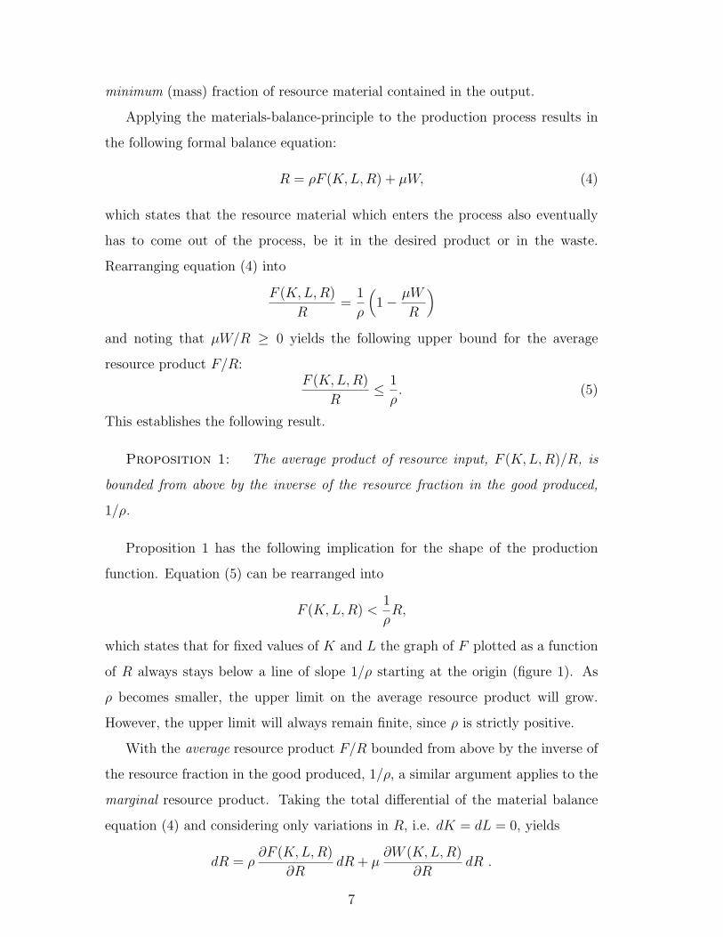
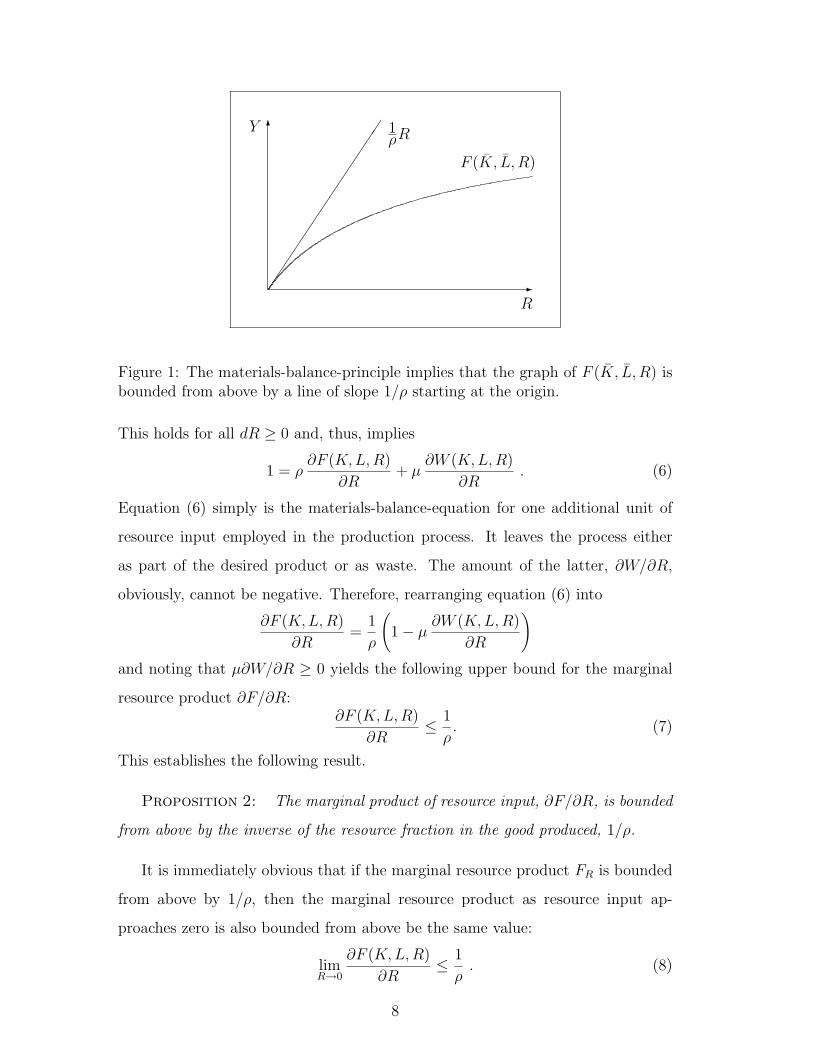
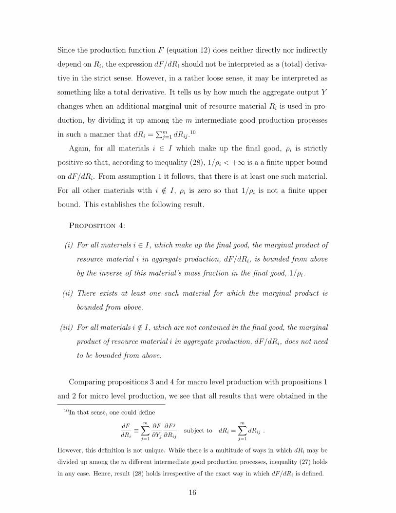
Proposition 1 has the following implication for the shape of the production
function. Equation (5) can be rearranged into
F (K, L,R) <1
ρR,
which states that for fixed values of K and L the graph of F plotted as a function
of R always stays below a line of slope 1/ρ starting at the origin (figure 1). As
ρ becomes smaller, the upper limit on the average resource product will grow.
However, the upper limit will always remain finite, since ρ is strictly positive.
With the average resource product F/R bounded from above by the inverse of
the resource fraction in the good produced, 1/ρ, a similar argument applies to the
marginal resource product. Taking the total differential of the material balance
equation (4) and considering only variations in R, i.e. dK = dL = 0, yields
dR = ρ∂F (K, L,R)
∂RdR + µ
∂W (K, L,R)
∂RdR .
7
6Y
-R
1
ρR
F (K, L, R)
Figure 1: The materials-balance-principle implies that the graph of F (K, L, R) isbounded from above by a line of slope 1/ρ starting at the origin.
This holds for all dR ≥ 0 and, thus, implies
1 = ρ∂F (K, L, R)
∂R+ µ
∂W (K, L, R)
∂R. (6)
Equation (6) simply is the materials-balance-equation for one additional unit of
resource input employed in the production process. It leaves the process either
as part of the desired product or as waste. The amount of the latter, ∂W/∂R,
obviously, cannot be negative. Therefore, rearranging equation (6) into
∂F (K, L,R)
∂R=
1
ρ
(1− µ
∂W (K, L,R)
∂R
)
and noting that µ∂W/∂R ≥ 0 yields the following upper bound for the marginal
resource product ∂F/∂R:∂F (K, L,R)
∂R≤ 1
ρ. (7)
This establishes the following result.
Proposition 2: The marginal product of resource input, ∂F/∂R, is bounded
from above by the inverse of the resource fraction in the good produced, 1/ρ.
It is immediately obvious that if the marginal resource product FR is bounded
from above by 1/ρ, then the marginal resource product as resource input ap-
proaches zero is also bounded from above be the same value:
limR→0
∂F (K, L,R)
∂R≤ 1
ρ. (8)
8
This is the content of the following corollary to proposition 2.
Corollary: The marginal product of resource input as resource input ap-
proaches zero is bounded from above by the inverse of the resource fraction in the
good produced, 1/ρ.
By this corollary it becomes apparent that the Inada conditions (in whatever
form), when applied to a micro level production function with material resource
inputs, are inconsistent with the Materials-Balance-Principle.
The intuition behind the simple formal exercise carried out in this section is
that matter cannot be created and, consequently, the produced output cannot
contain more of some material than has been supplied as input. If, for instance,
one needs 100 gram of some resource material in order to produce 1 kilogram of
a good (ρ = 1/10), then, out of 1 kilogram of the resource one can produce at
maximum (i.e. with no waste) 10 kilogram of output. This means, the average as
well as the marginal resource product is bounded from above by 10 (= 1/ρ).
4 Thermodynamic limits to resource productiv-
ity at the macro level
The simple model of production specified by equation (3) was confined to the
description of one particular micro level production process and one particular
natural resource. In order to analyse how the thermodynamic law of conservation
of mass may restrict aggregate production, we should think of production in a more
general way:
• There are many different natural resources, such that one can substitute
from one resource to another, in order to avoid thermodynamic constraints
on micro level production, such as conditions (5) or (7), to become binding.
• Production of an aggregate output, such as an all purpose commodity or
GDP, is a multi-level process. On a first level, a number of different interme-
diate goods are produced from elementary resources (micro level production).
9
On a second level, the final output is produced from the intermediate goods
(macro level production).6
• In the production of final output there is scope for substitution between the
input of different intermediate goods.
In such a setting, there is plenty of scope for substitution both between different
elementary resource materials and between production processes. The question
then is: To what extent do thermodynamic constraints on micro level production
processes, such as conditions (5) or (7), carry over to the macro level? And how
do the laws of thermodynamics restrict aggregate production in such a general
setting?
To answer these questions, consider the following model of production of an
all purpose commodity from intermediate goods, which are themselves produced
from a variety of elementary natural resources. There are n different elementary
natural resources, numbered by i = 1, . . . , n. Assume that this is a complete and
exhaustive list of material resources actually or potentially used in production.
For example, one may think of this list of natural resources as the complete list
of known chemical elements, in which case n = 112.7 These are used as inputs in
the production of m different intermediate goods, each of which is produced by
a single process of production, numbered by j = 1, . . . , m. Production of theses
intermediates is described by production functions
Yj = F j(Kj, Lj, R1j, . . . , Rnj) for all j = 1, . . . , m, (9)
where Kj and Lj denote input of capital and labor into production of intermediate
good j. Similarly, Rij (with i = 1, . . . , n and j = 1, . . . , m) denotes input of
6In general, aggregate production may be over more than two levels. But the essential insights
can already be grasped from considering a two-level-system.7As of 2003, there are 112 known chemical elements, 83 of which are naturally occurring. Ex-
amples include hydrogen, carbon, oxygen, iron, copper, aluminum, gold and uranium. Elements
113 through 118 are known to exist, but are not yet discovered (IUPAC 2003).
10
resource material i into production of intermediate good j. Then,
Ri =m∑
j=1
Rij (10)
is the total amount of resource material i utilized in production. Each production
process F j also yields a certain amount of waste, Wj.
Let ρij with 0 ≤ ρij ≤ 1 denote the (mass) fraction of resource material i
contained in the intermediate good j, and µij with 0 ≤ µij ≤ 1 the (mass) fraction
of resource material i contained in the waste from producing intermediate good j.
Note that ρij will be zero if the intermediate good j does not contain any material
of type i. This may include cases in which some resource material has been used in,
or is even essential for, the production of the intermediate, say as a catalyst, yet the
material is not contained in the good produced. Nonetheless, every intermediate
good j – as long as it is a material good and not an immaterial service – contains
some amount of some of the materials, while not containing anything of other
materials. In order to make this distinction explicit, let
Ij = {i | ρij > 0} ⊆ {1, . . . , n} (11)
be the set of all resources which make up – as far as material content goes – the
intermediate good j. The complement set Ij = {1, . . . , n} \ Ij then denotes the
set of all resources which are not materially contained in the intermediate good j.
The final good, an all purpose commodity, is produced from capital K, labor
L and the intermediate goods Yj (with j = 1, . . . , m):
Y = F (K, L, Y1, . . . , Ym), (12)
where Yj (with j = 1, . . . ,m) denotes input of intermediate good j as produced on
the first level of production (equation 9). On this level, elementary resources do not
enter directly into production, but only indirectly insofar as they are embedded in
the intermediates.8 The final good production function (12) can be interpreted as
an aggregate production function of the economy, specifying how the final good is
8This assumption, which is also quite plausible, only serves to simplify the notation and does
not restrict the validity of results. It could easily be relaxed.
11
produced from elementary resources, when the Yj’s are replaced by the respective
micro level production functions (equations 9).
The production of the final good also yields a certain amount of waste, W . Let
ρi with 0 ≤ ρi ≤ 1 denote the (mass) fraction of resource material i contained
in the final output, and µi with 0 ≤ µi ≤ 1 the (mass) fraction of the resource
material i contained in the waste. Note that ρi will be zero if the final good
does not contain any material of type i. Nevertheless, the final good – as long
as it is a material good and not an immaterial service – contains some amount
of some of the materials, while not containing anything of other materials. For
example, a passenger car may contain aluminum, carbon and thallium, but no gold
or plutonium. In order to make this distinction explicit, let
I = {i | ρi > 0} ⊆ {1, . . . , n} (13)
be the set of all resources which make up – as far as material content goes – the
final good. The complement set I = {1, . . . , n} \ I then denotes the set of all
resources which are not materially contained in the final good. Assume that the
final good is material, that is, it contains at least one type of material.
Assumption 1: I is non-empty.
With this setting and notation, propositions 1 and 2 derived in section 3 above
can obviously be translated and generalized into the following statement:
Lemma 1: The thermodynamic law of conservation of mass implies that the
micro level production functions F j(Kj, Lj, R1j, . . . , Rnj) for all j = 1, . . . , m have
the following properties:
F j(Kj, Lj, R1j, . . . , Rnj)
Rij
≤ 1
ρij
and
∂F j(Kj, Lj, R1j, . . . , Rnj)
∂Rij
≤ 1
ρij
for all i ∈ Ij.
In words, the average and marginal resource product of resource material i in
producing the intermediate good j is bounded from above by 1/ρij in all cases
12
where material i is contained in intermediate good j. If, in contrast, material i is
not contained in intermediate good j, the average and marginal resource product
of resource material i do not need to be bounded from above.9
Considering the overall two-level production system, the formal balance condi-
tions for resource material i (for all i = 1, . . . , n) then read as follows:
Ri =m∑
j=1
Rij , (14)
Rij = ρijFj(Kj, Lj, R1j, . . . , Rnj) + µijWj
for all j = 1, . . . , m , (15)m∑
j=1
ρijFj(Kj, Lj, R1j, . . . , Rnj) = ρiF (K,L, Y1, . . . , Ym) + µiW . (16)
Equation (14) states that the total amount of resource material i employed in
production, Ri, may be used in any of the m production processes for intermediate
goods. Equation (15) expresses conservation of mass of resource material i on the
first level of production in all of the m intermediate good production processes: the
total amount of material utilized in one of these processes, Rij, leaves the process
either as part of the intermediate good j or as part of the waste generated by
that process. Equation (16) expresses conservation of mass on the second level of
production: resource material i enters production of the final product indirectly,
namely embedded in the m intermediate goods, each of which has a material
content of that material of ρijYj. It leaves the production process either as part of
the final good or as part of the waste generated by that process. Summing balance
equation (15) over all micro level processes j, adding balance equation (16) for the
macro level, and using (14) yields an overall balance condition for material i:
Ri = ρiF (K, L, Y1, . . . , Ym) + µiW +m∑
j=1
µijWj . (17)
This condition states that the material utilized in production, Ri, leaves the two-
level production system either as part of the final good, or as part of the waste
generated by the final good production process, or as part of the waste generated
in any of the m intermediate good production processes.
9Of course, in the latter case they may still be bounded from above for reasons other than
thermodynamic necessity.
13
Rearranging equation (17) into
F (K,L, Y1, . . . , Ym)
Ri
=1
ρi
1− µiW
Ri
−
m∑j=1
µijWj
Ri
(18)
and noting that µiW/Ri ≥ 0 as well as∑m
j=1 µijWj/Rj ≥ 0, the following inequality
holds:F (K,L, Y1, . . . , Ym)
Ri
≤ 1
ρi
. (19)
For all materials i ∈ I which make up the final good, ρi is strictly positive so that
1/ρi < +∞ is a a finite upper bound for the average resource product of material i
in aggregate production, F/Ri. From assumption 1 it follows that there is at least
one such material. For all other materials with i /∈ I, ρi is zero so that 1/ρi is not
a finite upper bound. This establishes the following result.
Proposition 3:
(i) For all materials i ∈ I, which make up the final good, the average product of
resource material i in aggregate production, F/Ri, is bounded from above by
the inverse of this material’s mass fraction in the final good, 1/ρi.
(ii) There exists at least one such material for which the average product is
bounded from above.
(iii) For all materials i /∈ I, which are not contained in the final good, the average
product of resource material i in aggregate production, F/Ri, does not need
to be bounded from above.
In order to derive an analogue statement about the marginal resource products,
take the total differential of the material balance equation (17) for material i, with
the Yj in production function F replaced my the intermediate good production
functions F j (equations 9), and consider only variations in resource material i (i.e.
dK = dL = 0, dKj = dLj = 0 for all j and dRi′j = 0 for all i′ 6= i):
dRi = ρi
m∑
j=1
∂F
∂Yj
∂F j
∂Rij
dRij + µi
m∑
j=1
∂W
∂Yj
∂F j
∂Rij
dRij +m∑
j=1
µij∂Wj
∂Rij
dRij . (20)
14
From balance equation (14) it follows that
dRi =m∑
j=1
dRij . (21)
Replacing dRi in equation (20) by expression (21) and rearranging terms yields
m∑
j=1
[1− ρi
∂F
∂Yj
∂F j
∂Rij
− µi∂W
∂Yj
∂F j
∂Rij
− µij∂Wj
∂Rij
]dRij = 0 . (22)
This holds for all dRij ≥ 0 and, thus, implies that the term in brackets equals
zero. This can be rearranged into
∂F
∂Yj
∂F j
∂Rij
=1
ρi
[1− µi
∂W
∂Yj
∂F j
∂Rij
− µij∂Wj
∂Rij
]. (23)
Noting that the second and third term in brackets are non-negative yields the
following inequality, which holds for all i and j:
∂F
∂Yj
∂F j
∂Rij
≤ 1
ρi
. (24)
On the other hand, taking the total differential of the defining equation for pro-
duction function F (equation 12), with the Yj in production function F replaced
my the intermediate good production functions F j (equations 9), and considering
only variations in resource material i (i.e. dK = dL = 0, dKj = dLj = 0 for all j
and dRi′j = 0 for all i′ 6= i), yields:
dF =m∑
j=1
∂F
∂Yj
∂F j
∂Rij
dRij . (25)
From (25) one obtains, using inequality (24) and equation (21)
dF =m∑
j=1
∂F
∂Yj
∂F j
∂Rij
dRij ≤m∑
j=1
1
ρi
dRij =1
ρi
m∑
j=1
dRij =1
ρi
dRi , (26)
so that we have the following inequality:
dF ≤ 1
ρi
dRi . (27)
Interpreting this inequality for differentials as an algebraic expression and rear-
ranging finally yields:dF
dRi
≤ 1
ρi
. (28)
15
Since the production function F (equation 12) does neither directly nor indirectly
depend on Ri, the expression dF/dRi should not be interpreted as a (total) deriva-
tive in the strict sense. However, in a rather loose sense, it may be interpreted as
something like a total derivative. It tells us by how much the aggregate output Y
changes when an additional marginal unit of resource material Ri is used in pro-
duction, by dividing it up among the m intermediate good production processes
in such a manner that dRi =∑m
j=1 dRij.10
Again, for all materials i ∈ I which make up the final good, ρi is strictly
positive so that, according to inequality (28), 1/ρi < +∞ is a a finite upper bound
on dF/dRi. From assumption 1 it follows, that there is at least one such material.
For all other materials with i /∈ I, ρi is zero so that 1/ρi is not a finite upper
bound. This establishes the following result.
Proposition 4:
(i) For all materials i ∈ I, which make up the final good, the marginal product of
resource material i in aggregate production, dF/dRi, is bounded from above
by the inverse of this material’s mass fraction in the final good, 1/ρi.
(ii) There exists at least one such material for which the marginal product is
bounded from above.
(iii) For all materials i /∈ I, which are not contained in the final good, the marginal
product of resource material i in aggregate production, dF/dRi, does not need
to be bounded from above.
Comparing propositions 3 and 4 for macro level production with propositions 1
and 2 for micro level production, we see that all results that were obtained in the
10In that sense, one could define
dF
dRi≡
m∑
j=1
∂F
∂Yj
∂F j
∂Rijsubject to dRi =
m∑
j=1
dRij .
However, this definition is not unique. While there is a multitude of ways in which dRi may be
divided up among the m different intermediate good production processes, inequality (27) holds
in any case. Hence, result (28) holds irrespective of the exact way in which dF/dRi is defined.
16
simple micro-level setting essentially carry over to the general two-level-multi-
resources-multi-processes setting. The only qualification is that the boundedness-
results only hold for materials in the set I which make up the final good.
5 Discussion
It has been shown that the Inada conditions, when applied to material resource
inputs, may be inconsistent with the thermodynamic law of conservation of mass,
the so-called Materials-Balance-Principle. In particular, the analysis has revealed
that the average and marginal product of a natural resource material in aggregate
production are bounded from above due to the thermodynamic law of mass con-
servation if the final good, an all-purpose commodity, contains this material. An
upper bound is given by the inverse of this material’s mass fraction in the final
good.
The analysis was based on a model of multi-level production where different
intermediate goods are produced from different elementary resources, and an all-
purpose final commodity is produced from these intermediates. Note that no
limits on substitution between resource materials or between intermediate products
have been assumed. Another thing to note is that the upper bound specified by
inequalities (19) and (28) is certainly not the lowest upper bound, but comes out
of a more or less crude estimation (from equations (18), (26) to inequalities (19),
(27)). For that reason, the upper bound given here does not depend on any model
parameters other than ρi.
When discussing the relevance of these results for the natural-resources-and-
economic-growth-debate, the crucial questions are:
(i) How many, and which natural resource materials are elements of the set I?
That is, what are the natural resource materials that make up, materially,
the final good?
(ii) What is these materials’ mass fraction ρi in the final good?
(iii) How do the set I and the relevant parameter values ρi change over time?
17
It is probably the difference in opinion on these questions which make a differ-
ence between the “optimists” and the “pessimists” in the discussion about the
thermodynamic limits to economic growth.
This analysis has revealed that there are stringent thermodynamic limits to
resource productivity in aggregate production for a number of natural resource
materials. The analysis has also revealed that not all resource materials need to
be limiting. Hence, the overall conclusion is that the question of thermodynamic
limits to economic growth requires a detailed investigation, with separate analyses
and results for each material. This shifts the focus of the debate from overall
growth to the more detailed level of factor substitution and structural change.
References
[1] Anderson, C.L. (1987). The production process: inputs and wastes. Journal
of Environmental Economics and Management 14: 1-12.
[2] Ayres, R.U. (1999). Materials, economics and the environment. In: J.C.J.M.
van den Bergh (ed.), Handbook of Environmental and Resource Economics,
Edward Elgar, Cheltenham, pp. 867-894.
[3] Barelli, P. and S. de Abreu Pessoa (2003). Inada conditions imply that pro-
duction function must be asymptotically Cobb-Douglas. Economics Letters
81: 361-363.
[4] Baumgartner, S. (2000). Ambivalent Joint Production and the Natural Envi-
ronment. An Economic and Thermodynamic Analysis. Physica-Verlag, Hei-
delberg.
[5] Beckerman, W. (1999). A pro-growth perspective.In: J.C.J.M. van den Bergh
(ed.), Handbook of Environmental and Resource Economics, Edward Elgar,
Cheltenham, pp. 622-634.
[6] Berry, R.S., P. Salomon and G. Heal (1978). On a relation between economic
and thermodynamic optima. Resources and Energy 1: 125-137.
18
[7] Boulding, K.E. (1966). The economics of the coming spaceship Earth. In:
Jarrett (ed.), Environmental QUality in a Growing Economy, Johns-Hopkins-
University Press, Baltimore.
[8] Daly, H.E. (1977/1991). Steady State Economics. The Economics of Biophys-
ical Equilibrium and Moral Growth. First edition 1977, second edition 1991.
W.H. Freeman, San Francisco.
[9] Daly, H.E. (1997a). Special issue: “The Contribution of Nicholas Georgescu-
Roegen”. Ecological Economics 22(3).
[10] Daly, H.E. (1997b). Georgescu-Roegen versus Solow/Stiglitz. Ecological Eco-
nomics 22(3): 261-266.
[11] Dasgupta, P. and G. Heal (1974). The optimal depletion of exhaustible re-
sources. Review of Economic Studies 41 (Symposium on the Economics of
Exhaustible Resources): 3-28.
[12] Dasgupta, P. and G. Heal (1979). Economic Theory and Exhaustible Re-
sources. Cambridge University Press, Cambridge, UK.
[13] Dyckhoff, H. (1983). Inada-Bedingungen und Eigenschaften der neoklassis-
chen Produktionsfunktion. Zeitschrift fur die gesamte Staatswissenschaft –
Journal of Institutional and Theoretical Economics 139(1): 146-154.
[14] Fare, R. and D. Primont (2002). Inada conditions and the law of diminishing
returns. International Journal of Business and Economics 1(1): 1-8.
[15] Georgescu-Roegen, N. (1971). The Entropy Law and the Economic Process.
Harvard University Press, Cambridge, MA.
[16] Hoel, M. (1978). Resource extraction and recycling with environmental costs.
Journal of Environmental Economics and Management 5: 220-235.
[17] Inada, K.I. (1963). On a two-sector-model of economic growth: comments and
a generalization. Review of Economic Studies 30: 119-127.
19
[18] IUPAC – International Union of Pure and Applied Chemistry (2003).
http://www.iupac.org, searched on 6 October 2003.
[19] Kondepudi, D. and I. Prigogine (1998). Modern Thermodynamics. From Heat
Engines to Dissipative Structures. Wiley, New York.
[20] Kurz, H.D. and N. Salvadori (2003). Fund-flow versus flow-flow in production
theory: Reflections on Georgescu-Roegen’s contribution. Journal of Economic
Behavior and Organization 51: 487-505.
[21] Maler, K.G. (1974). Environmental Economics: A Theoretical Inquiry. The
Johns Hopkins University Press, Baltimore.
[22] Pethig, R. (2003). The ‘materials balance approach’ to pollution: its origin,
implications and acceptance. Universitat Siegen, Volkswirtschaftliche Diskus-
sionsbeitrage 105-03.
[23] Sandelin, B. (1976). On the origin of the Cobb Douglas production function.
Economy and History 19: 117-123.
[24] Schulze, W.D. (1974). The optimal use of non-renewable resources: The the-
ory of extraction. Journal of Environmental Economics and Management 1:
53-73.
[25] Schumpeter, J.A. (1954). History of Economic Analysis. Oxford University
Press, New York.
[26] Shephard, R.W. (1970). Theory of Cost and Production Functions. Princeton
University Press, Princeton.
[27] Solow, R.M. (1956). A contribution to the theory of economic growth. Quar-
terly Journal of Eocnomics 70: 65-94.
[28] Solow, R.M. (1974). Intergenerational equity and exhaustible resources. Re-
view of Economic Studies 41 (Symposium on the Economics of Exhaustible
Resources): 29-45.
20
[29] Solow, R.M. (1997). Georgescu-Roegen versus Solow/Stiglitz – Reply. Ecolog-
ical Economcis 22: 267-268.
[30] Smith, V.L. (1977). Control theory applied to natural and environmental re-
sources – an exposition. Journal of Environmental Economics and Manage-
ment 4: 1-24.
[31] Smulders, S. (1999). Endogenous growth theory and the environment. In:
J.C.J.M. van den Bergh (ed.), Handbook of Environmental and Resource Eco-
nomics, Edward Elgar, Cheltenham, pp. 610-621.
[32] Stiglitz, J. (1974). Growth with exhaustible natural resources: Efficient and
optimal growth paths. Review of Economic Studies 41 (Symposium on the
Economics of Exhaustible Resources): 123-152.
[33] Stiglitz, J.E. (1997). Georgescu-Roegen versus Solow/Stiglitz – Reply. Eco-
logical Economcis 22: 269-270.
[34] Swan, T.W. (1956). Economic growth and capital accumulation. Economic
Record 32: 334-361.
[35] Weinstein, M.C. and R.J. Zeckhauser (1974). Use patterns for depletable and
recyclable resources. Review of Economic Studies 41 (Symposium on the Eco-
nomics of Exhaustible Resources): 67-88.
[36] Wicksell, K. (1893). Uber Wert, Kapital und Rente nach den neueren na-
tionalokonomischen Theorien. Gustav Fischer, Jena.
[37] Wicksteed, P.H. ([1894]1992). The Coordination of the Laws of Distribution.
First published in 1894. Revised edition, with an introduction by I. Steedman.
Edward Elgar, Aldershot.
21