the incapacitation effect of incarceration: evidence from ...ftp.iza.org/dp6360.pdf · the...
TRANSCRIPT

DI
SC
US
SI
ON
P
AP
ER
S
ER
IE
S
Forschungsinstitut zur Zukunft der ArbeitInstitute for the Study of Labor
The Incapacitation Effect of Incarceration:Evidence from Several Italian Collective Pardons
IZA DP No. 6360
February 2012
Alessandro BarbarinoGiovanni Mastrobuoni

The Incapacitation Effect of Incarceration:
Evidence from Several Italian Collective Pardons
Alessandro Barbarino Federal Reserve Board
Giovanni Mastrobuoni
Collegio Carlo Alberto, CeRP and IZA
Discussion Paper No. 6360 February 2012
IZA
P.O. Box 7240 53072 Bonn
Germany
Phone: +49-228-3894-0 Fax: +49-228-3894-180
E-mail: [email protected]
Any opinions expressed here are those of the author(s) and not those of IZA. Research published in this series may include views on policy, but the institute itself takes no institutional policy positions. The Institute for the Study of Labor (IZA) in Bonn is a local and virtual international research center and a place of communication between science, politics and business. IZA is an independent nonprofit organization supported by Deutsche Post Foundation. The center is associated with the University of Bonn and offers a stimulating research environment through its international network, workshops and conferences, data service, project support, research visits and doctoral program. IZA engages in (i) original and internationally competitive research in all fields of labor economics, (ii) development of policy concepts, and (iii) dissemination of research results and concepts to the interested public. IZA Discussion Papers often represent preliminary work and are circulated to encourage discussion. Citation of such a paper should account for its provisional character. A revised version may be available directly from the author.

IZA Discussion Paper No. 6360 February 2012
ABSTRACT
The Incapacitation Effect of Incarceration: Evidence from Several Italian Collective Pardons*
We estimate the “incapacitation effect” on crime using variation in Italian prison population driven by eight collective pardons passed between 1962 and 1995. The prison releases are sudden – within one day –, very large – up to 35 percent of the entire prison population – and happen nationwide. Exploiting this quasi-natural experiment we break the simultaneity of crime and prisoners as in Levitt (1996) and, in addition, use the national character of the pardons to separately identify incapacitation from changes in deterrence. The elasticity of total crime with respect to incapacitation is between -20 and -35 percent. A cost-benefit analysis suggests that Italy’s prison population is below its optimal level. JEL Classification: K40, K42, H11 Keywords: crime, pardon, amnesty, deterrence, incapacitation Corresponding author: Giovanni Mastrobuoni Collegio Carlo Alberto Via Real Collegio 30 Moncalieri (TO), 10024 Italy E-mail: [email protected]
* We would like to thank Josh Angrist, David Autor, Michele Belot, Paolo Buonanno, Francesco Drago, Chris Flinn, Maria Guadalupe, Luigi Guiso, Andrea Ichino, Stepan Jurajda, Peter Katuscak, Alex Mas, Bhashkar Mazumder, Nicola Persico, Filippo Taddei, Pietro Vertova, and Till Von Wachter for their useful comments. We thank the Italian Econometric Association for their Carlo Giannini Prize. We would also like to thank seminar participants at Boston University, CERGE-EI, Collegio Carlo Alberto, Einaudi Institute for Economics and Finance, European University Institute, Federal Reserve Board lunch seminar, Federal Reserve System Applied Micro Conference, MIT, Tilburg University, University of Bologna, and University of Tor Vergata. We also thank Riccardo Marselli and Marco Vannini for providing the judiciary crime statistics, Franco Turetta from the Italian Statistical Office for providing the data on police activities, Marco Iaconis from the Osservatorio sulla sicurezza fisica of the Italian association of banks for providing the data on bank robberies, Elvira Barletta from the Department of Penitentiary Administration for preparing the budgetary data. Rute Mendes has provided excellent research assistance. Any opinions expressed here are those of the authors and not those of the Federal Reserve Board and of the Collegio Carlo Alberto.

1 Introduction
Despite the recent consensus by researchers on crime and punishment that elements of the
judicial system, such as increased police forces and incarceration rates, are effective in reducing
crime (Levitt, 2004), there is no consensus on the size of the reduction nor on the exact channels
through which such reduction is achieved (Donohue, 2007). This paper provides a detailed
empirical analysis of both.
In the United States the response to the unprecedented spike in crime rates in the 90s has
been an increase in policing and, to a much larger extent, in incarceration. The US prison
population is now the highest in the world.1 Moreover, the large stock of inmates has the
potential to create a second crime wave as sentences expire (Raphael and Stoll, 2004; Duggan,
2004). These facts call into question the effectiveness of a further expansion in incarceration
as opposed to alternative policies and prompts a further inquiry on the marginal benefit of
imprisonment.
To this end it is crucial not only to have a precise measurement of the total effect of
incarceration on crime, but also to disentangle the deterrence effect of corrective measures
from their incapacitating effect (Shavell, 1987). Indeed, recent studies attempt to isolate either
the deterrence effect or the incapacitation effect exploiting detailed aspects or policies of the
judiciary system. For instance, Kuziemko (2006) exploits parole boards in Georgia, Owens
(2009) sentence enhancements in Maryland, Kessler and Levitt (1999) sentence enhancements
in California, Helland and Tabarrok (2007) three strikes laws in California, and Weisburd et al.
(2008) different strategies to enforce payments of court ordered fines.2
In the same spirit our paper focuses on collective pardons, release policies based on general
criteria that lead to large reductions in prison population. In particular, we study a series of
1Police forces increased around 20 percent over the last 20 years, while due to harsher punishments incar-ceration rates increased fourfold in the U.S. over the last 30 years. In 2005 there were 737 inmates per 100,000US residents (International Center for Prison Studies 2007) compared with a world average of 166 per 100,000and an average among European Community member states of 135 Raphael and Stoll (2009)). McCrary (n.d.)warns that prison population is not in steady state yet and that the reforms of the past 5-30 years have still toproduce their full-fledged effects.
2In the literature review we try to provide the reader with a brief summary of such work.
3

pardons enacted in Italy during the years 1962-1995, that lead to the release of prisoners whose
residual sentence length was less than a given number of years, usually two or three. It turns
out that these policies generate a large variation in prison population across time and regions.
For instance, the last collective pardon, passed on July 31, 2006, led within a day to the release
of 22,000 inmates, around 30 percent of the total (DAP, 2006).
These sudden changes can be used to break the classical simultaneity between crime and
prisoners (Levitt, 1996). Unlike most other policy experiments found in the literature, pardons
generate nationwide, immediate, measurable and large changes in prison population that, we
argue below, are not related to other factors that influence crime.
A first identification strategy, based on monthly time-series crime data and the exact date
the pardon gets passed leads to an estimated elasticity of crime with respect to prison population
of respectively 15 percent. The identification of the total elasticity (deterrence + incapacita-
tion) with the monthly time series estimates requires few assumptions, since it is based on
discontinuous changes in crime rates following pardons measured at a high frequency. However
the elasticity is only approximate since we do not have monthly data on prison population.
By contrast, the identification based on yearly panel data allows us to control for deterrence
funneled by criminals expectations and allows us to disentangle deterrence from incapacitation.
Given that immediately after a pardon gets passed criminals should be less prone to commit
crimes–a) the next pardon is unlikely to happen very soon, and b) pardoned sentences might
be added to the a new sentence (see Drago et al., 2009)–, the incapacitation effect should be
larger than the total effect. This is what we find. The elasticity of total crimes based on the
panel data, equal to 35 percent, is indeed larger than the one based on monthly data.
We classify the different types of deterrence that might arise in our experiment. Crimi-
nals expectations are potentially an important channel through which deterrence is at work.
Criminals might try to predict the timing of pardons and change their behavior accordingly.
Hence failing to control for criminals’ expectations might bias the estimates towards zero since
changes in criminals expectations might make the variation induced by the policy endogenous.
We control for criminals’ expectations making use of the nationwide nature of pardons. The
4

intuition is the following: pardons are national laws that are outside the control of regional
administrations and are homogeneous across regions. As such, they should affect criminal ex-
pectations (and deterrence) in a similar way across the country. Controlling for time absorbs
the deterrence effect that works through criminals expectations. Notice that if pardons were
regional we would not be able to control for this type of deterrence. We consider additional
types of deterrence that might be associated with our experiment such as congestion and crowd-
ing out effects but we find that criminal expectations are the most important channel through
which deterrence is at work.
Levitt (1996) is the closest paper in the literature to this work. In his paper a set of indicator
variables capture the status of overcrowding litigation, which generate an exogenous variation in
the US prison population. Sometimes court decisions led to fewer offenders sentenced to prison
terms, sometimes to early release programs and other times to the construction of new prison
facilities and to a reallocation of prisoners across institutions. He estimates the combined effect
of deterrence and incapacitation using a quasi-natural experiment based on aggregate U.S.
states-level data and his estimated elasticities are indeed larger than our estimates.
With our estimates in hand we then move on to study the efficiency level of the Italian
prison population. Heterogeneity of criminal types generates a distribution of criminal-specific
social costs. The sum of these social costs per released prisoner are approximately 3 times as
large as the cost of keeping him in prison, indicating that Italy has a prison population that is
below its optimal level. The mainly unselective pardons that have been enacted recently are
thus very inefficient, as the release of potential criminals has a social cost greater than the cost
of incarceration.3 Indeed, in case of overcrowding an expansion in prison capacity should be
preferred to an unselective pardon, and has lately been planned by the Italian government.
Research using data from different countries helps evaluating the robustness of the extant
3In the spirit of this “selective incapacitation,” the Italian penal code establishes that pardons and amnestiesshould not be given to recidivist, recurrent, or career criminals (art. 151). Despite this article, in the 1990and 2006 pardons and in the 1990 amnesty, the legislators decided to extend the benefits to career criminals.Moreover, because of evidence that criminal activity decreases with age, the legislators have sometimes increasedthe number of pardoned years for older criminals (usually defined as being older than 65 or 70 years of age).Other preferred treatments for elderly inmates were introduced in 1974 (law n. 220).
5

findings that are all based on US data and can support useful cross-country comparisons at
times where many researchers wonder about the optimal size of the US prison population.4
1.1 Related Literature
In this section we provide a brief review of the literature on the relationship between crime and
incarceration that is close to the issues raised in our paper.
Studies on the Correlation of Crime and Prison Population – Several papers have tried to
estimate the effect of prison population on crime. Early studies do not control for endogeneity
and use state level time series data and regressions. Stemen (2007) reviews these studies:
the elasticity of crime with respect to incarceration range from positive figures down to -28
percent. Not controlling for endogeneity clearly biases the results upwards. Among the most
notable studies Marvell and Moody (1994) proceed by rejecting that crime Granger causes
prison population, and later estimate an elasticity of crime with respect to prison population
of -0.16. Spelman (1994) finds similar effects.5 The studies above fail to account for the
simultaneity between crime and imprisonment. Given that when for whatever reason crime
rises the prison population will mechanically increase the simultaneity pushes the estimated
correlations between crime rates and incarceration rates towards zero. Levitt (1996) controls
for the simultaneity using an instrumental variables (IV) approach and finds elasticities that
are two to three times larger than before.
Studies that Isolate Deterrence – Among the many studies that focus on deterrence it
is worth mentioning Kessler and Levitt (1999) who exploit sentence enhancements to isolate
deterrence from incapacitation. Helland and Tabarrok (2007) use the deterrent effect of Cali-
fornia’s “three-strike” law to isolate deterrence. Weisburd et al. (2008) use a randomized field
trial of alternative strategies for incentivising the payment of court ordered fines to estimate
deterrence. Levitt (1998) isolates deterrence based on the discontinuity in punitiveness at the
4Few researchers have explored Italian data using an economic approach, with Buonanno et al. (2009),Buonanno et al. (2008), Drago et al. (2009), and Marselli and Vannini (1997) being rare exceptions.
5See also Raphael and Winter-Ebmer (2001), Marvell and Moody (1997), Donohue and Levitt (2001), andSpelman (2000, 2005).
6
age of majority and finds evidence of it. In contrast, Lee and McCrary (2005) examine a lon-
gitudinal database of individual level arrest records in Florida. They take advantage of data
on the exact date of birth of arrestees and look for discontinuous changes in offending right at
the age of cutoff using a regression discontinuity design, but find no sizable declines at the age
of majority. Drago et al. (2009) exploit random variation in sentence length due to a recent
collective pardon to isolate deterrence.
Studies that Isolate Incapacitation – Owens (2009) uses a one-time exogenous change in
sentence enhancements for 23-25 year-old inmates in the State of Maryland to isolate incapaci-
tation but she estimates the effect that incarceration has on individual recidivism, rather than
crime. Recidivism might not be a proper measure of crime if arrested criminals tend to commit
different types of crimes or a different number of crimes than non arrested ones. It might also
not properly capture congestion and replacement effects:6 the increased supply of criminals
due to pardons might reduce the probability of being detected, and consequently attract new
entrants in the criminal market. In contrast, released criminals might also drive some of the
old criminals out of the market, making the total effect on crime ambiguous.Whenever several
prisoners are released at once peer effects might be at work as well. Moreover, whenever large
numbers of prisoners are released the prison administration might face more binding constraints
in assisting released prisoners to provide job counseling, accommodation, etc. We later test for
this additional effect that depends on the size of the released prison population by splitting the
sample based on the group of regions with releases above or below the median.
Finally, a special issue of Quantitative Criminology (2007) contains a thorough overview of
studies on incapacitation.
Studies on Pardons – Only a few papers have studied the effect of pardons on crime. The
reason is that most empirical research on the criminal justice system focuses on the United
States, where pardons are rare (Levitt and Miles, 2004) and release small numbers of inmates.
(Mocan and Gittings, 2001) estimates the deterrence effect of gubernatorial pardons of persons
6See Cook (1986), Freeman (1999) and Miles and Ludwig (2007) for a more thorough discussion of thereplacement and spillover effects.
7

on death row and finds that three additional pardons generate 1 to 1.5 additional homicides.
Kuziemko (2006) studies parole boards in Georgia and exploits overcrowding litigation and a
collective pardon of 900 inmates to find out the relationship between time served and recidi-
vism and the efficiency of parole boards but she does not concentrate on the estimation of
incapacitation nor on the evaluation of pardons.
In Italy, despite the recurrent use of pardons, there has been only one empirical study on
the relationship between pardons and crime. The study Tartaglione (1978) headed by a judge
that was killed in that same year by the Red Brigade terrorist group, finds that after the
1954, 1959, 1966, and 1970 pardons, national changes in crime tend to be above average. The
exceptions are the 1963 pardon, in which only one year was pardoned, and the 1968 pardon,
which applied only to certain crimes committed during student demonstrations. The study
also documents that pardoned inmates have a recidivism rate of 31.2 percent, which is not
that different from 32.9 percent, the recidivism rate of prisoners who are released at the end
of their term. Standard errors are not shown, so we do not know whether these differences
are significant or not. The judges who worked on this pioneering study did not use regression
methods, which makes it impracticable to analyze the link between prison population and
crime or to use regional variation in the fraction of released prisoners. The judges also made
no attempt to value the monetary cost of the increased crime, or to separate the incapacitation
effect from the total effect.
2 Italy’s Collective Pardons and Prison Population
Historical remarks – Pardons and amnesties are deeply rooted in the Italian legislative history
and culture. Between the unification of Italy in 1865 and the defeat of Mussolini in 1943
there have been approximately 200 pardons or amnesties, though some of these were just fiscal
pardons, or amnesties for very specific crimes. Some of these pardons were aimed at easing
social tensions, others were passed to magnify the royal family. A pardon was passed when the
Prince of Naples was born (1869) and one when he got married (1896). Other pardons followed
8

the colonization of Eritrea, Somalia, Cyrenaica, Tripolitania and later Ethiopia, the peace
treaty between Italy and Austria (1919), the annexation of Slavic territories in the North-East
of Italy. Though sometimes even local tensions led to pardons (wood thefts in the Montello
region, illegal cutting of olive and mulberry trees (1920), crimes committed in occupied Greece,
etc.) The use of amnesties and pardons in Italy has been the norm, and the fact that an entire
article of the 1945 Constitution is devoted to these acts (art. 79) shows that after World War II
nothing changed. Between 1945 and today there have been more than a dozen pardons (mostly
coupled with amnesties). Although these were firstly aimed at reconciling a politically divided
nation, in more recent times an additional goal has been to reduce prison overcrowding.
Legal definition – Starting in 1992, collective amnesties and pardons in Italy have been
issued by the legislators with an absolute majority requirement of two-thirds (constitutional
law n.6 of 1992). Before that year, the President could issue them but only after they had
been mandated by a simple majority of the parliament. The main difference between amnesties
and pardons is that amnesties eliminate both the sentence and the crime, as if they never
happened, whereas pardons eliminate only part of the sentence. Given that Italian prosecutors
are required by law to investigate all felonies (art. 112 of the Constitution), pardons are
usually followed by amnesties.7 Otherwise, prosecutors would have to spend time and effort
investigating pardoned crimes, even if it was impossible to actually punish the perpetrators.
Another difference between the two is that whenever the pardoned prisoner recommits a crime
within five years, the commuted prison term gets added to the new term.8 Amnesties, instead,
are permanent.9 10
7The 2006 pardon was an exception to this rule.8The incapacitation that we estimate represents, therefore, a lower bound of the typical incapacitation.
Drago et al. (2009) exploit this rule to identify the deterrence effect of prison.9The great majority of pardoned prisoners are convicted criminals, though some might be in preventive
detention with an expected sentence that is below the maximum number of pardoned years. For example,in 2006 when the number of pardoned years was three, 10.7 percent of the prisoners that were freed were inpreventive detention (Marietti, 2006).
10Pardons and amnesties also reduce the number of arrestees who are subject to restrictive measures that aredifferent from imprisonment namely, social work outside prison, semi-liberty, and house arrest. Between 1975,the year in which these measures were introduced in Italy, and 1995, 19 percent of apprehended criminals (oralleged criminals) were subject to these alternative measures. It has been shown that recidivism rates for theseindividuals are significantly lower than those for prisoners (Santoro and Tucci, 2004) and that some of theseindividuals might commit crimes even while subject to these alternative measures. Nevertheless, changes in
9

Overcrowding – The left panel of Figure 1 shows that the official prison capacity (measured
as the number of beds per 100,000 Italian citizens) declined between 1962 and 1975, significantly
reducing the cushion between the total prison population and the total capacity. Although 81
new prisons were build between 1971 and 2003, 87 older and obsolete ones were dismissed during
the same period(de Franciscis, 2003). As a result, between 1975 and 1991, prison capacity was
basically flat at almost 50 beds per 100,000 residents. Only in more recent times has capacity
increased. In 1983, as a result of flat capacity and a steady increase in crime, the prison
population exceeded the “official” capacity (even if aggregated at the national level) for the
first time. If necessary the prison administration can add new beds to existing cells, to reach
what is defined as “tolerable” capacity. The 1986 pardon was the first one to solve a situation of
overcrowding. Partly because of the tougher majority requirements, 16 years passed between
the most recent pardon, in 2006, and the pardon before that. During the same period, the
prison population tripled from about 20,000 to 60,000, dropping to about 35,000 after the 2006
pardon.
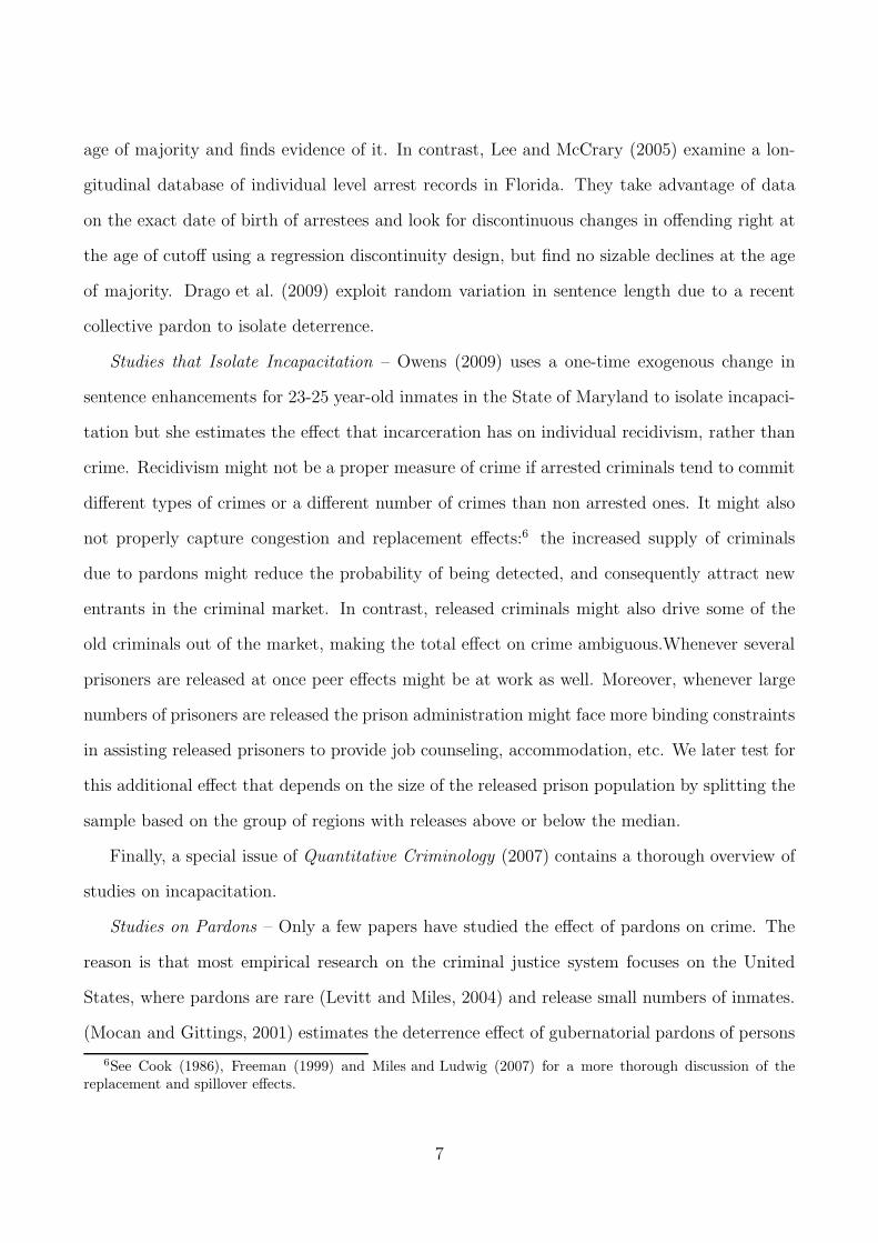
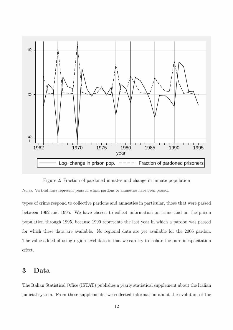
Pardons and Prison Population – Figure 2 shows the log-changes in prison population and
the fraction of pardoned prisoners.11 It is evident that collective pardons induce an almost
one-for-one change in prison population. Overall the fraction of inmates that gets freed can be
as high as 35 percent, and it sometimes reaches 80 percent in single regions. But the effect of
pardons on prison population appears to be short-lived. Within one year, the inmate population
recovers more than half of the size of the initial jump. Between 1959 and 1995, for example, the
inmate population increased, on average, by 449 inmates per year, but with large fluctuations
that were driven by the pardons. The inmate population decreases by an average of 3,700
inmates after pardons, but increases by an average of 2,944 inmates immediately afterwards. In
all other years the average increase is by 1,165 inmates. In other words, in the year immediately
after the pardons, and excluding the year of the pardon, the inmate population grows two and
a half times faster.
crime might be due in part to these additional pardoned individuals.11The Italian Statistical Office (ISTAT) groups together pardoned and amnestied prisoners.
10

2040
6080
100
1000
2000
3000
4000
5000
Tot
al n
umbe
r of
crim
es
1962 1970 1975 1980 1985 1990 1995year
Total number of crimes Prison populationPrison capacity
Pris
on p
op. a
nd c
apac
ity
Figure 1: End of the year prison population, prison capacity, and the total number of crimes
Notes: Vertical lines represent years in which pardons or amnesties have been passed.
Pardons generate also variation across regions. Table 1 shows the fraction of pardoned
inmates across regions. Table 2 shows, for example, that in the Abruzzo and Molise regions,
aggregated because of data limitations, the 1966 pardon freed 85 percent of the inmate pop-
ulation, while in Sardinia only 38 percent left the jail. The 1968 pardon, which applied to
crimes committed during student demonstrations, led to a release of very few prisoners. Two
years later,instead, in five regions—namely, Abruzzo, Molise, Friuli-Venezia Giulia, Liguria,
and Trentino-Alto Adige—more than 70 percent of prisoners were freed. Later pardons have
led to fewer releases. The last pardon in our sample happened in 1990, as the judicial data
about the 2006 pardon are not available yet.
The next section presents the additional crime data that are used to measure how other
11
−.5
0.5
1962 1970 1975 1980 1985 1990 1995year
Log−change in prison pop. Fraction of pardoned prisoners
Figure 2: Fraction of pardoned inmates and change in inmate population
Notes: Vertical lines represent years in which pardons or amnesties have been passed.
types of crime respond to collective pardons and amnesties in particular, those that were passed
between 1962 and 1995. We have chosen to collect information on crime and on the prison
population through 1995, because 1990 represents the last year in which a pardon was passed
for which these data are available. No regional data are yet available for the 2006 pardon.
The value added of using region level data is that we can try to isolate the pure incapacitation
effect.
3 Data
The Italian Statistical Office (ISTAT) publishes a yearly statistical supplement about the Italian
judicial system. From these supplements, we collected information about the evolution of the
12

prison population and about crime for 20 Italian regions between 1962 and 1995. ISTAT
publishes two sets of crime statistics: those collected directly by the police corps (Polizia
di Stato, Carabinieri and Guardia di Finanza) from people’s complaints (Le Statistiche della
Delittuosita), and those collected by the judicial system (Le Statistiche della Criminalita) when
the penal prosecution, which in Italy is mandatory, starts. The two sets of statistics differ
whenever at least one of the following things happen: i) the initial judge decides that the
complaint does not depict a crime; ii) the judicial activity is delayed with respect to the time
that the crime was committed; iii) a crime is reported to public officials who do not belong to
the police corps. Since the exact timing of our statistic is important in most of our analysis
we use crime as measured by the police. When single crime categories are unavailable in the
police data, and as a robustness check, we also use the judicial statistics.12
Table 3 shows the summary statistics of the variable that we use. Variables are weighted by
the resident population. Between 1962 and 1995, there were on average 42 inmates per 100,000
residents. Levitt (1996) shows that during a similar time frame in the United States the inmate
population was 168, exactly four times as large as in Italy. Our statistics indicate that the
total amount of crimes per year per 100,000 residents was 1,983. This number is significantly
smaller than Levitt’s number for the United States (approximately 5,000), which might be
due to underreporting. In 1984, ISTAT started separating reported crimes into more specific
categories. Some categories are identical to those reported by Levitt, and allow a comparison
between Italy and the United States. Burglaries seem less frequent in Italy (285 versus 1,200),
and so seem larcenies (265 versus 2,700), though the definition of these crimes might differ as
well. For motor vehicle thefts, where the definition is clear, and where underreporting and
multiple offenses are less frequent, the two countries are similar: 420 per 100,000 residents in
Italy and 402 in the United States.
Full-year Equivalence – Given that some released prisoners get rearrested within a year,
we would like to estimate how crime rates vary immediately after a pardon gets enacted.
12In 1984, ISTAT changed the categorization of crimes in the police statistics, providing a more detailed crimecategorization. Instead, for the judicial data we can use a sample on single crime categories that starts in 1970(Marselli and Vannini, 1997).
13

But pardons and amnesties are sometimes passed in the middle of the year, and we have no
access to monthly regional data. Fortunately, we can use the date on which the pardon gets
passed to adjust the change in the prison population and the number of pardoned prisoners
to produce “full-year equivalent” pardoned prisoners—that is, prisoners who can potentially
commit crimes for a whole year. Take, for example, the 1978 pardon. The law was issued on
August 5. Assuming that after the pardon criminal activity was uniformly distributed over
time, recidivist prisoners would have been able to commit crimes for five months in 1978. One
way to take this timing into account and produce “full-year equivalent” prisoners is to reduce
the number of pardoned prisoners by 7/12 in the year of the pardon and add these prisoners
to the year after the pardon, year in which they can potentially commit crimes for the whole
year.13
More generally, based on the day of the year, d, on which the pardon becomes active,
full-year equivalent pardoned prisoners are
PARDONED∗
t,r =365− d
365PARDONEDt,r
in the year of the pardon and
PARDONED∗
t,r =d
365PARDONEDt,r−1 + PARDONEDt,r
in the year after the pardon, and
PARDONED∗
t,r = PARDONEDt,r
in all other years. We also adjust the prison population accordingly. Later we are also going to
see how robust our results are when we use different ways to adjust prison flows to the dating
of pardons.
13In 1990, the amnesty occurred in April, while the pardon occurred in December. As a result, the weightis going to be the average of the two periods weighted by the fraction of released prisoners who got releasedbecause of the pardon (80 percent) and because of the amnesty (20 percent) (Censis, 2006).
14

4 The Estimated Incapacitation Effect
4.1 Identification using monthly time-series variation
As for how pardons affect crime, ideally one would compare monthly crime-level statistics
with the monthly number of pardoned criminals. Monthly data on crime are available for
the years 1962-1983, but not for prison population. The top left panel of Figure 3 shows
the monthly data, while all other panels simply zoom into a two year window around each
pardon. From the figures one can see that crime rates tend to increase right after pardons
get passed (the horizontal lines). A simple comparison of pre/post differences, meaning the
distance between the horizontal lines, shows that apart from the last panel crime rates tend to
be larger immediately after the pardons than immediately before. The estimated differences
shown in the title are significantly different from zero. The discontinuity is less clear cut in
1963 and 1982, years where the released fraction of prison population has been relatively small
(approximately 10 percent). Later we will show that overall these differences are statistically
significant even when first-differencing the data to control for preexisting trends.
For the 2006 pardon we also have data on monthly prison population, which we match
with data on a specific crime, bank robberies. The two panels of Figure 4 show the number
of bank robberies per 100 bank branches between January 2004 and December 2007. The
vertical line represents the end of July, when the prison population dropped from 60,710 to
38,847 (-37 percent). The right panel shows the estimated regression discontinuity using the
region level monthly data with a cubic term of time. Within a month the number of bank
robberies jumped by 0.31 per 100 branches (with a standard error of 0.07) from around 0.5
to 0.8. Given that prison population decreased by 37 percent the estimated elasticity is close
-160 percent (0.3/0.5/0.37). The dotted line shows the estimated discontinuity when we use 12
month averages just before and after the pardon. The estimated change is equal to 0.18 (with
a standard error of 0.04). The estimated elasticity on a yearly basis is closer to 1.
We should keep in mind that such an elasticity represents the sum of the (negative) inca-
pacitation and (likely positive) deterrence effects. We speculate that the net deterrence effect
15

5010
015
020
0to
tal c
rimes
1960m1 1965m1 1970m1 1975m1 1980m1 1985m1date
6065
7075
80
1962m1 1962m7 1963m1 1963m7 1964m1date
total crimes Fitted values
break=4 (1.9)
7075
8085
90
1965m7 1966m1 1966m7 1967m1 1967m7date
total crimes Fitted values
break=6.1 (1.4)75
8085
9095
100
1969m7 1970m1 1970m7 1971m1 1971m7date
total crimes Fitted values
break=12.1 (1.2)
140
150
160
170
180
1977m7 1978m1 1978m7 1979m1 1979m7date
total crimes Fitted values
break=12.1 (2.6)
155
160
165
170
175
180
1981m1 1981m7 1982m1 1982m7 1983m1date
total crimes Fitted values
break=−8.1 (2.6)
Figure 3: Monthly crime rates per 100,000 residents, and structural breaks)
Notes: The break is estimated using a two year window centered at each pardon. The standard errors are inparentheses. Vertical lines represent months in which pardons or amnesties have been passed.
16

is positive since immediately after a pardon gets passed criminals do not expect a new pardon
to be passed in the near future and inmates that were released because of a pardon would risk
to see their old sentence added to the new one if they got rearrested.
.4.4
5.5
.55
.6P
rison
pop
. (10
0.00
0)
.4.5
.6.7
.8R
obbe
ries
per
100
bran
ches
Month of pardon1/04 1/05 1/06 1/07 1/08End of month/Year
Robberies per 100 branches Prison pop. (100.000).4
.5.6
.7.8
Ban
k ro
bber
ies
per
100
bank
s
Month of pardon1/04 1/05 1/06 1/07 1/08End of month/Year
Robberies per 100 branches Predicted robberies
The estimated RD=0.31 (SE=0.07)
Figure 4: Monthly bank robberies per 100 branches
We just showed that bank robberies had a sizeable increase after the 2006 pardon. Should
we expect similar increases for other kinds of crime? In other words, who are the prisoners that
are typically released? The last column of Table 4 shows the changes in prison population for
different types of criminals, while the distribution and the rank of the different types of crimes
committed by the inmates are shown in the remaining columns. Overall the distribution of
the type of crimes committed by prisoners serving jail just before and just after the July 2006
pardon are very similar. Most changes in prison population are close to the overall 37 percent
decline. Since Mafia related crimes are excluded from pardons, criminals who had committed
these crimes were less likely to exit jail in August. Seventeen percent of them did leave jail,
probably, by having pardoned the part of their crime that was not related to the “mafia-type
criminal association” felony (Associazione per Delinquere di Tipo Mafioso, art. 416 of the
penal codex). The 2006 pardon did not apply to some drug-related criminals, which is why
their decline is smaller than the average decline. Criminals who committed crimes against
persons are less likely to exit jail than criminals that have committed crimes against wealth,
but the differences are small. We do not have the month-by-month distribution of crime types
for the other pardons but a quick look at past pardon bills shows that historically very few
17
crime categories have been excluded from such clemency bills, suggesting that differences are
likely to be negligible. This means that in terms of criminal background pardoned inmates are
similar to those inmates that are released after serving their entire sentence. Later, when we use
pardoned inmates to instrument changes in prison population, the resulting estimates should
therefore represent average incapacitation effects rather than incapacitation effects related to
some specific inmates.
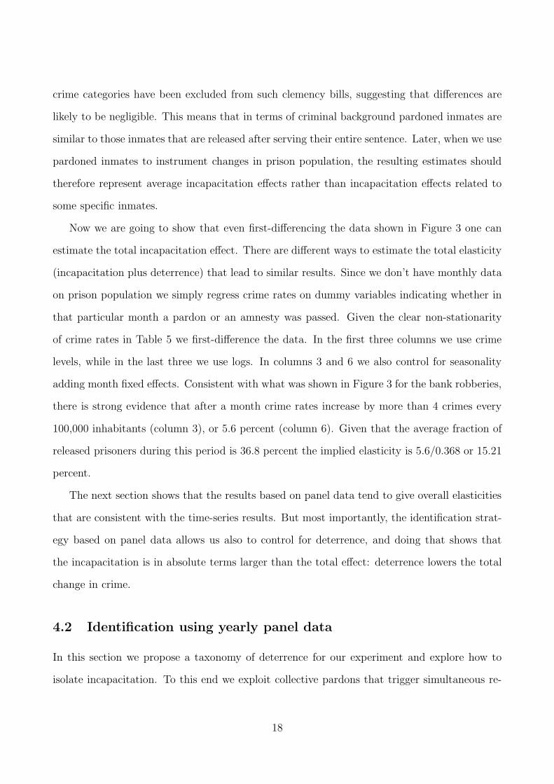
Now we are going to show that even first-differencing the data shown in Figure 3 one can
estimate the total incapacitation effect. There are different ways to estimate the total elasticity
(incapacitation plus deterrence) that lead to similar results. Since we don’t have monthly data
on prison population we simply regress crime rates on dummy variables indicating whether in
that particular month a pardon or an amnesty was passed. Given the clear non-stationarity
of crime rates in Table 5 we first-difference the data. In the first three columns we use crime
levels, while in the last three we use logs. In columns 3 and 6 we also control for seasonality
adding month fixed effects. Consistent with what was shown in Figure 3 for the bank robberies,
there is strong evidence that after a month crime rates increase by more than 4 crimes every
100,000 inhabitants (column 3), or 5.6 percent (column 6). Given that the average fraction of
released prisoners during this period is 36.8 percent the implied elasticity is 5.6/0.368 or 15.21
percent.
The next section shows that the results based on panel data tend to give overall elasticities
that are consistent with the time-series results. But most importantly, the identification strat-
egy based on panel data allows us also to control for deterrence, and doing that shows that
the incapacitation is in absolute terms larger than the total effect: deterrence lowers the total
change in crime.
4.2 Identification using yearly panel data
In this section we propose a taxonomy of deterrence for our experiment and explore how to
isolate incapacitation. To this end we exploit collective pardons that trigger simultaneous re-
18
gional variations in crime that arguably are exogenous and unrelated to factors that influence
crime. We also explicitly allow criminals to respond positively to expected future pardons
through changes in deterrence. Hence, our identification strategy revolves around instrument-
ing changes in regional prison population with the number of pardoned prisoners released in
the region with the extra precaution of controlling for deterrence funneled by expectations. Con-
trolling for time allows us to kill two birds with a stone: on the one hand, time controls purify
our estimates from expectation-driven deterrence effects leaving us with the sole incapacitation
effect; on the other hand, they neutralize the danger that criminals’ expectations about pardons
make these policies be as if they were endogenous.
Long-term deterrence effect – As mentioned pardons might generate changes in deterrence
through criminals expectations. Since pardons reduce the expected sanction, everything else
being equal, we should expect crime rates to be higher in a society that occasionally makes
use of them. Given the unavailability of a counterfactual Italian society without pardons, this
effect is hard to estimate but is going to be absorbed by the constant term.
Pre-pardon deterrence effect – Criminals might also try to strategically time (around the
time of the pardon) their criminal activity in order to minimize their expected sanction (pre-
pardon deterrence). This effect is severely dampened by the rule that pardons only apply to
crimes committed up to a specific date, usually three to six months before the signing of the
law. The risk of committing a crime that is too close to a pardon, and therefore excluded from
the pardon, is likely to significantly reduce the incentive to commit pardonable crimes shortly
before the law passes.
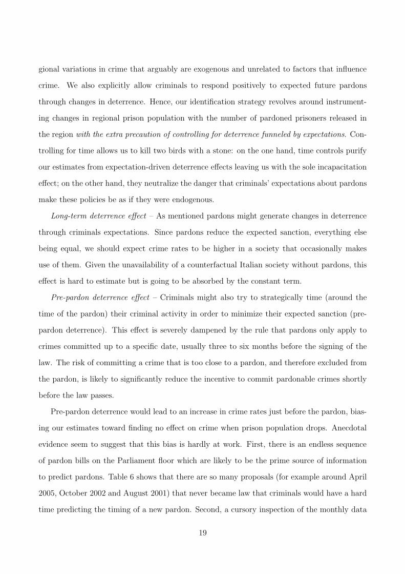
Pre-pardon deterrence would lead to an increase in crime rates just before the pardon, bias-
ing our estimates toward finding no effect on crime when prison population drops. Anecdotal
evidence seem to suggest that this bias is hardly at work. First, there is an endless sequence
of pardon bills on the Parliament floor which are likely to be the prime source of information
to predict pardons. Table 6 shows that there are so many proposals (for example around April
2005, October 2002 and August 2001) that never became law that criminals would have a hard
time predicting the timing of a new pardon. Second, a cursory inspection of the monthly data
19

available for the 2006 pardon shown in Figure 4 would exclude that in that year the short term
deterrence effect is at work. Before July 2006 bank robberies were actually trending down,
which is not consistent with criminals expecting a new pardon and timing their crimes accord-
ingly. Moreover, monthly data allow us to try to predict the implementation of a pardon using
the information available until right before it is passed. In particular Table 7 shows that using
monthly data it is impossible to predict the exact timing of pardons based on crime rates during
the past 3, 6, or 12 months. Using high frequency data one can isolate very narrow intervals
around pardons, showing that the estimated discontinuities are not subject to simultaneity bias.
There is no evidence that pardon are passed depending on recent patterns of crime.
Post-pardon deterrence effect – Expectations on pardons are likely to be updated immedi-
ately after pardons get passed. And this is the largest and most worrisome deterrence effect
because criminals are going to be less likely to commit crimes: i) they know that the next
pardon is unlikely to happen within their expected sentence length, and ii) released prisoners
would see their pardoned sentenced added to the new one if they were rearrested.14 The lowered
propensity to commit crimes immediately after a pardon would again lead to underestimating
incapacitation. Fortunately these laws are nationwide laws (outside the control of regional ad-
ministrations, and homogeneous across regions when implemented), meaning that the implied
changes in expectations are arguably the same across the country and will be fully absorbed
by time controls.
Assuming that once we control for time effects there is enough variation left in the number
of released prisoners across regions, the structure of our experiment allow us to control for
post-pardon deterrence, isolating incapacitation. The variation in the prison population that
we exploit is the variation in the fraction of prisoners who are pardoned across regions at a
given point in time. This fraction depends on the distribution of the residual prison time of
the inmate population, which at the time of the pardon is certainly predetermined.15 16
14Drago et al. (2009) use this rule to isolate deterrence effects.15Kuziemko (2006) uses a similar variation to estimate the effect of time served on recidivism.16The link between regional prison population and regional crime depends crucially on the law establishing
that each arrested criminal must first be incarcerated in prisons that are located inside the competent judicialjurisdiction where the crime has been committed (Competenza per Territorio, Article 8 of the Codice di Procedura
20

The variation in number of released inmates comes from two sources: 1.) for a given crime,
variation in the residual sentence length that is due to variations in the date of arrest or in the
date of conviction, depending on whether the judge decides to keep the criminal in jail during
his trial;17 2.) for a given date of conviction, variation in the residual sentence length which
might or might not be due to differences in the distribution of crime seriousness.18
Policing, congestion and replacement effects – There is also the possibility that the release
of a large mass of prisoners might change other factors that affect deterrence, like increased
policing or other changes in police actions, that in our model corresponds to changes in pt,r. But
these effects are measurable and we think that we have fairly good proxies for these changes.
There might also be congestion and/or replacement effects: on one side, the increased supply
of criminals due to pardons might reduce the probability of being detected, and consequently
attract new entrants in the criminal market; one the other side, released criminals might drive
some of the old criminals out of the market, making the total effect on crime ambiguous. But
again, these effects would generate non-linearities between crime and prison population that
we can test.
Other potential sources of biases – Another possible source of endogeneity of our instrument
is the possibility that increased crime rates may lead, if no new prisons are built, to prison
overcrowding, which may lead to a collective release: this chain of events would make our
policy endogenous (not necessarily through criminals’ expectations rather through the national
Government reaction function).19 We already showed that pardons do not seem to be related
to previous crime rates. And since pardons are unlikely to depend on year to year changes in
crime we adopt the precaution of differencing the data, working with changes in crime instead
Penale) and might later be transferred to a prison that is closest to where the respective family resides (Article42 of the 26 of July 1975 n. 354 law). Each region has one or more jurisdictions, with the exception of the ValleD’Aosta and Piedmont regions which share the jurisdiction of Torino.
17Preliminary judges can keep suspected criminals in jail if at least one of these three risks is present: i)reiteration of the same crime, ii) escape, and iii) removal of the evidence
18It has been shown that even under federal sentencing guidelines the same crime might be judged differentlyby different judges (Anderson et al., 1999) and the ability of lawyers is also likely to influence the sentencelength for the same kind of crime.
19Tartaglione (1978) argues that pardons in the 60s and 70s were difficult to justify other than for a politicalpreference for clemency, but Figure 1 does show that after 1982 prisons started to be overcrowded.
21

of levels.20
Regions that had and might still have higher crime rates might simply release more prisoners
so that the fraction of pardoned prisoners in a region might depend on the level of crime in
the previous period in the same region. If this was the case regional lagged crime rates would
be able to predict the fraction of released prisoners. Table 8 tests whether this is the case by
regressing the fraction of pardoned prisoners at time t on the logarithm of crime at time t− 1
using a sample of regions where at least 1, 5, or 10 percent of prisoners are released. No matter
the sample we choose the coefficient is quite precisely estimated to be close to zero. Thus, there
is no evidence that regions with higher crime rates at time t − 1 release a larger fraction of
prisoners, meaning that a compositional bias is unlikely to arise.
Average effects and local effects – With a variation in the distribution of crime seriousness
that differs across regions and over time our estimated incapacitation effect might not measure
the average effect, but rather a local one. If, for example, in Piedmont criminals commit
frequent but petty crimes, while in Sicily crimes are less frequent but more serious, a pardon
would tend to release more prisoners from Piedmont. The incapacitation effect would, therefore,
give more weight to crimes which are on average less serious. The opposite would be true if
criminals who are caught recidivating commit crimes more frequently, because these criminals
receive sentences that are increased by at least a third (art. 81 of the Italian penal codex). We
neutralize the variation in the distribution of crime seriousness by focusing on specific types of
crime and by interacting the average (log) sentence length of the same crime types with the
fraction of pardoned prisoners.21 We exploit the regional variation given that approximately
90 percent of inmates get arrested in the region they reside (ISTAT, 1961-1995).22
The Behavioral Model – Let us introduce a simple model of criminal behavior to disci-
20Differencing the data is also important in case crime levels and prison population are non-stationary. Aregression in levels might then give spurious results.
21Ideally we would like to measure the region-specific and crime specific average sentence length of pardonedprisoners and not the one of the whole prison population, though the two are likely to be correlated sincepardoned prisoners are part of the prison population. The two measures would also be correlated within regionsif sentence lengths contained a judge-specific fixed effect, though we do not have data to test for the existenceof these fixed effects.
22We do not find evidence of criminal spillovers to contiguous regions.
22

pline our reasoning and to formalize the mechanics of deterrence and incapacitation that leads
naturally to our empirical specification. The model, a revised version of Kessler and Levitt
(1999)’s model, can be viewed as a reduced form of the search model of crime developed in
Lee and McCrary (2005) and McCrary (n.d.). Suppose criminal i (the mass of criminals is nor-
malized to 1 by dividing the number of criminals by the regional population), who is ex-ante
identical to all other criminals, faces the following dichotomic problem at time t:
maxE[bi,t − pt,rJ(St)|It]Ci,t
where Ci,t takes the value 1 if the criminal chooses to commit the crime; the return from
crime, bi,t, is, for simplicity, uniformly distributed between 0 and B; the joint probability of
apprehension and conviction varies across regions and the distribution of the disutility from
jail, J(St), depends on the expected sentence length, conditional on the information available
up to time t, including information about possible future pardons.
Differences in the probability of apprehension and conviction are assumed to be temporary,
with mean E[pt,r] = pt. Later in the empirical specification we deal with possible systematic
differences by i) controlling for proxies of p, ii) differencing the data, and iii) controlling for
regional fixed effects. Information about pardons, I, does not vary across regions. The criminal
will commit a crime if bi,t > ptE[J(St)|It] = ptJt.
In the simplified case of a sentence length of one year, the law of motion of criminals is
Ct,r = 1︸︷︷︸
total criminal pop
−
[ptJt
B(1− pt−1,rCt−1,r)
]
︸ ︷︷ ︸
fraction deterred of free population
− pt−1,rCt−1,r︸ ︷︷ ︸
fraction incapacitated
.
It is possible to relax, in a reduced-form approach, the assumption that sentence length, S,
equals 1. If S is equal to 2 the model becomes
Ct,r = 1︸︷︷︸
total criminal pop
−
[ptJt
B(1− pt−1,rCt−1,r − pt−2,rCt−2,r)
]
︸ ︷︷ ︸
fraction deterred of free population
− pt−1,rCt−1,r − pt−2,rCt−2,r︸ ︷︷ ︸
fraction incapacitated
,
23

and, after rearranging,
Ct = 1−ptJt
B−
(ptJt
Bpt−1 − pt−1
)
Ct−1 −
(ptJt
Rpt−2 − pt−2
)
Ct−2.
Generalizing to sentence lengths up to duration Smax gives the following:
Ct,r = 1−ptJt
B−
Smax∑
s=1
(ptJt
Bpt−s − pt−s
)
Ct−s,r .
Now let us introduce a pardon. The effect of pardoning Z years is to free Wt,r criminals at
the beginning of period t, 1− ptJtB
of whom will recommit crimes during the year:
Ct,r = 1−ptJt
B
(
1−
Smax∑
s=1
pt−s,rCt−s,r +Wt,r
)
−
Smax∑
s=1
pt−s,rCt−s,r +Wt,r .
We allow the pardon to have an effect on future expected sentence lengths, Jt. The difference
between the scenarios with and without a pardon will be:
Ct,r − Ct,r =
(
ptJt
B−
ptJt
B
)(
1−Smax∑
s=1
pt−s,rCt−s,r
)
+Wt,r
(
1−ptJt
B
)
. (1)
The first summand measures the change in crime due to deterrence, the second summand the
change due to incapacitation. In particular,(
1− ptJtB
)
measures the fraction of crimes that are
attributable to the released criminals, the incapacitation effect.
The Empirical Model – Given our discussions above, we are ready to set up our empirical
model. We do not observe the counterfactual criminal scenario of a “pardon year” without
a pardon. In our empirical specification we proxy for the counterfactual of crime using years
that are contiguous to the pardon. The dependent variable is going to be the first difference
in crime rates. To isolate the incapacitation effect, we need to realize that in Italy pardons are
nationwide policies and that the deterrence effect is, therefore, unlikely to vary across regions.
If time effects, and time-varying variables capture changes in the deterrence effect, then the
coefficient on the number of pardoned prisoners captures the incapacitation effect, 1− ptJtB
.
24

When we analyze the effect of the prison population on total crime the model is
∆CRIMEt,r = β∆PRISONt,r + f(t) + δ′Xt,r + γr + ǫt,r,
where the main variables are expressed in logarithmic terms. Changes in prison population
are instrumented using the fraction of pardoned prisoners. Notice that the IV’s reduced-form
equation in levels,
∆CRIMEt,r = βPARDONEDt,r + ˜f(t) + δ′Xt,r + γr + ǫt,r
is directly related to equation 1, with the counterfactual scenario being replaced with the
scenario in the previous year. The term f(t)+ γr+ δ′Xt,r is supposed to capture the deterrence
effect and isolate the incapacitation effect β = 1− ptJtB
. All variables except the average sentence
length are first-differenced (which controls for systematic differences in the levels) and all but
the average sentence length and the probabilities are expressed in terms of 100,000 residents.
All regressions include regional fixed effects, which control for systematic differences in trends
(for example, long-term changes in the probability of apprehension and conviction, or changes
in the attractiveness of the legal labor market, etc.), though results without regional fixed
effects are almost identical.
Although yearly fixed effects represent the methodologically correct tool to control for time
effect in our experiment, they absorb most of the variation in prison population that is needed
for identification when some years of data are unavailable. For this reason we introduce two
alternative ways to control for time effects. These controls should approximate the evolution
of criminals’ expectations.
In one specification we control for a cubic spline using three-year intervals; in the other, we
control for pardon-specific linear time trends. The use of splines assumes that criminals’ changes
in expectations evolve smoothly, without discontinuities. The complexity of the legislative
process that leads to pardons makes it difficult to forecast their date of enactment. Moreover,
25

criminals have to forecast not only the date of pardon but also its ending date of coverage.
This is likely to smooth the deterrence effect. In the other specification we use pardon-specific
linear trends, which assumes that criminals’ expectations jump to a new level in the year of the
pardon and evolve linearly thereafter. Both the constant term and the coefficient on time are
allowed to have a different evolution between each pair of pardons. In other words we simply
interact the constant term and time with pardon-specific dummy variables.
The different time controls are shown in Figure 5. The dotted line represents the estimate
of f(t) using year fixed effects. The estimated time effects are smoother when we use the three-
year cubic spline (solid line), especially during the 1980s and 1990s. But the pardon-specific
linear time trends (dashed line) are close to the fixed effects during the 1960s (it is the decade
with the highest number of pardons).
4.3 Results
Panel A of Table 9 shows the results of a first-stage regression of the change in prison population
on the number of pardoned prisoners. Only where time controls, f(t), are estimated using a
time fixed effects the fraction of pardoned prisoners lead to a reduction in the log of prison
population that is less than one. The F-statistic is simply the square of the t-statistic, and
is largely above the rule-of-thumb threshold level of 10 (Staiger and Stock, 1997). When we
control for year fixed effects (column 3), absorbing the nationwide variation in the number of
pardoned prisoners, the F-statistic is considerably lower, (0.376/0.0878)2 = 4.282 = 18.31, but
still above 10.
Panel B shows the reduced form regression, the Two Stage Least-Squares (IV) regression,
and the Ordinary Least Squares (OLS) regression results, where the dependent variable is
log-changes in crime.23 The reduced form regressions show patterns that are similar to the
23A special event took place in Italy in July 1990: the World Cup soccer tournament. In the 12 regionsthat hosted at least a game, log-changes in crime were, compared with the remaining regions, 12 percentagepoints larger in 1990 than in either 1989 or 1991 (p-value of 8 percent). Prisoner flows, however, did not seemto differ significantly because of the World Cup. To control for changes in crime that are due to the WorldCup, all regressions control for whether in 1990 the region hosted at least one World Cup game. We also add adummy equal to one for the region Umbria in 1991 to control for an apparent data error. After the 1990 pardonand amnesty Umbria is the only region that appears to have more pardoned prisoners in 1991 than in 1990.
26

−.1
0.1
.2E
stim
ate
of f(
t), i
n lo
gs
1965 1970 1975 1980 1985 1990 1995year
3Yr cubic spline Pardon specific lin. trendsYear dummies
Figure 5: Estimated time effects of the log of total crime (f(t))
Notes: Vertical lines represent years in which pardons or amnesties have been passed.
first stage results. The elasticities between crime and the fraction of pardon prisoners are
close to 20 percent with the only exception of the one estimated using time effects that is
approximately 50 percent lower. The IV estimates, which correspond to the ration between
the reduced form elasticities and the first stage elasticities tell us that a 10 percent reduction
in prison population increases the estimated number of crimes by between 1.84 percent and
3.52 percent. As expected the elasticities are closer to zero when we don’t control for time
fixed effects. Given that not controlling for f(t) the elasticities are quite close to the ones we
get using splines or pardon-specific time trends such functional form might not fully capture
changes in deterrence.24 The price one has to pay to add the year fixed effects is a considerable
Moreover, the number is larger than the total prison population (see Statistiche Giudiziarie Penali, Tavola 17.5,on page 629). Later we check whether the results are robust to the exclusion of this dummy variable.
24Notice that because of the simultaneity between crime and prison population OLS estimates are biased
27

loss of precision. When we use year dummies the p-value is 5.6 percent, considerably higher
than when using the other functional forms to approximate f(t). Because of data limitations
most of the analyses that follow use a smaller sample (fewer years), making the identification
that uses year dummies often impractical because of a lack of power. Since deterrence biases
the estimates toward zero we are going to stay on the conservative side using pardon-specific
time trends each time we need more precision. But we should keep in mind that we are most
likely understating the elasticity of crime with respect to prison population.
Robustness Checks – Table 10 addresses several initial robustness checks. Regressions (1)
and (4) are just replica of the ones shown in Table 9 shown for reference. The first represents
the one with pardon-specific trends, the second the one with year dummies. Regression (2)
replicates regression (1) but uses per capita jail population to weight the regressions instead
of the resident population. Regressions (3) and (5) show the elasticity when no weighting
is used. The results are definitely robust to different weighting procedures. Regression (6)
replicates regression (1) but clustering the standard errors by year instead of regions. Such
a clustering does increase the standard errors but the results are still significant. Regression
(7) adds regions fixed effects, allowing for region specific trends. Regression (8) shows that
using variables in levels instead of logs does not alter the results. Each additional released
criminal leads on average to 44 additional crimes. Regression (9) shows that the Umbria 1991
dummy does not alter the results. In regression (10) we compute full-year equivalent figures of
prison population and of the number of pardoned prisoners only for the first year and not in
the following year. The elasticities tend to be smaller because the initial months present the
most significant changes in crime. Not adjusting for the exact timing of the pardon, instead,
introduces sever measurement error and biases the results toward 0. Notice that since the
misclassification error is on average close to 50 percent (it is 0 whenever pardons happen at
the very beginning of the year and 1 whenever they happen at the very end) the coefficient is
approximately half the size of the elasticity in regression (1).
In regression (12) we test for non-linearities that might be driven by spillovers: congestion
toward zero.
28

or replacement effects. If criminals in regions with larger reductions in prison population have,
because of congestion, a smaller probability of detection, we should expect in absolute terms
the elasticities to be larger the larger the reduction in prison population. If instead a larger
release of prisoners emphasizes competition between criminals we should expect the opposite
to happen. Regression (12) adds the squared change in prison population around the average
change (instrumented using the squared fraction of pardoned prisoners). Adding the squared
term does not change the coefficient on the linear terms and the coefficient of the squared term
is not significantly different from zero. The coefficient is positive, which would be consistent
with replacement effects (the larger the reduction in prison population the smaller the change
in crime), but is not statistically significant.
Regressions (13) and (14) control for the lagged change in prison population and the lagged
changes in crime. If pardons were passed after crime rates have been particularly high, leading
to overcrowding, the elasticity estimated in regressions (1) to (12) might just capture correla-
tions between past levels of crime and thus prison population and current changes in prison
population. The results show that adding lagged values of prison population or changes in
prison population does not alter the results.25
Results for Total Crime Conditional on Other Covariates–In Table 11, we additionally
control for variables that might affect pardons and crime rates. Since some of the additional
controls are available only for the years 1985-1995, the sample size drops from 594 to 198.
For this reason we use pardon-specific time trends instead of year dummies to gain precision.
Despite the smaller sample size the estimates are precisely measured and are larger than the
elasticities estimated before, indicating that the incapacitation might have increased over time.
The elasticity drops from -19.6 to -30.7 percent. Less punitive amendments against recurrent
and professional criminals during the 1986 and 1990 pardons are likely to be main the reason
for this finding.
Changes in the probability that the perpetrator of the crime has been identified by the
25To make sure that the elasticity is not driven by a single region or a single pardon we estimate the elasticityof incapacitation excluding any single region or any single pardon the results were always statistically significantand of similar magnitude. The results are available upon request.
29

police represents one way to measure the productivity of law enforcement. Pardons might re-
duce the backlog of criminal cases and influence the productivity of law enforcement agencies.
An increase in this probability increases the expected sentence length and, therefore, might
influence crime. Controlling for sentence length and for changes in the probability that the
perpetrator is known leaves the IV elasticity practically unchanged. Changes in GDP are sup-
posed to proxy for legal opportunities of criminals, while changes in consumption are supposed
to capture illegal opportunities. In Column 3 we are also controlling for the change in the
fraction of population aged 15 to 35, the change in the population with high school degree and
the change in the population with university degree. Controlling for these opportunities does
not change the elasticity.
Police enforcement might respond strategically to the legislatures’s pardons. Depending
on their objective function, police officers might either increase or decrease their efforts to
apprehend criminals. On the one hand, the supply shock of criminals after a pardon is likely to
increase the probability of apprehension (p) and also police activity (A) if police officers’ goal is
to equate expected marginal benefits pB(A) to marginal costs C(A) and if BAA < 0, CAA > 0.
On the other hand, pardons are likely to weaken the police officers motivations and, therefore,
productivity. Pardons do more than nullify part of the officers’ past efforts. Criminals who
commit a crime before the pardon, but get arrested only after the pardon, can also benefit
from the pardon. Thus, even post-pardon arrests might end up with an early release. For
these reasons, in columns 4 and 9 we control for changes in the number of police officers and
for changes in the number of controlled people. The IV estimates are robust to this inclusion,
indicating, at least, that police activity does not change as abruptly as the inmate population.
Finally, we control for changes in the fraction of inmates staying in dormitories and for
the change in the rate of overcrowding (inmates divided by available beds). The reason is
that changes in prison quality might have a deterrence effect (Katz et al., 2003). Although the
change in the rate of overcrowding captures part of the variability that is due to the pardons,
there are again no significant changes, which suggests that pardons can be credibly treated as
exogenous and that there is no need to control for all these variables.
30

Results for Different Crime Categories – The results based on total crimes hides some
heterogeneity by crime types, in part because some crimes were not subject to pardons. We do
not have regional level data on changes in prison population by crime type, thus the independent
variable is going to be the same as the one used for total crimes. As we said, not all criminals
are pardoned and some restrictions always apply, and a number of crimes, like mafia-related
crimes, kidnappings, and sexual assaults, are always excluded from pardons.
But even if a criminal was convicted mainly for one of these crimes, and crime types are
recorded based on the most serious offense, he/she might still have committed additional par-
donable crimes. This is why Table 4 showed that during the last pardon even some mafia
members were released from prison. Also, even if none of the criminals that committed these
crimes were released, pardons might still influence these crimes if criminals do not fully special-
ize in given crimes. Excluded crimes are thus not a perfect placebo test, and Table 12 shows
that between 1984 and 1995 the coefficients on the types of crime that were explicitly excluded
from pardons, like mafia murders, kidnappings, and sexual assaults, tend to be less precisely
estimated. Bank robberies show an elasticity of 41 percent (almost significant at the 5 percent
level), and drug-related crimes have an elasticity of 52 percent, even though some drug-related
crimes were excluded from the 1990 pardon (but not from the 1990 amnesty).
The effects of pardons on larcenies are not significantly different from zero but Italian victim-
ization surveys show that only around half of those crimes get reported to the police.Muratore et al.
(2004). This measurement error is likely to inflate the standard errors of the estimated elas-
ticities. Indeed, motor vehicle theft which, unlike other thefts, are known to be measured with
high precision (the rates of reporting are close to 1 due to car insurance), have an elasticity of
27.8 percent. Row 14 and 15 of Table 12 shows that using judicial crime data instead of police
data strengthens the overall incapacitation effect (28 percent versus 21 percent). Given that
“judges for the initial investigation” (giudice delle indagini preliminari) are supposed to dismiss
all irrelevant cases before reporting a crime, this result is likely be due to increased precision in
the measurement of crime. Consistent with this possibility, the elasticity for all thefts, which
in include larcenies and burglaries, is equal to 40.8 percent. Frauds have an elasticity of 32.5
31

percent, and even the coefficient for homicides (murder and attempted murder) is significantly
different from zero (34.6 percent). The judiciary data has robberies, extortions and kidnappings
all under one category, and the elasticity is 25.5 percent.
In Section 4.2 we mentioned that regions whose prisoners serve on average shorter terms
release on average more prisoners when pardons get enacted. If these released prisoners tend to
commit crimes more frequently than average, it is important to control for the average sentence
length to rule out a spurious relationship between pardoned prisoners and crime. In Table 13 we
rerun the same specification as in Table 12 with in addition the demeaned average log sentence
length in the particular crime categories and its interaction with changes in prison population
instrumented with its interaction with the fraction of pardoned prisoners. The coefficient on the
interaction is never significant and the incapacitation effects are very close to the ones estimated
without controlling for sentence length, which indicates that selection is not a concern and that
most of the variability in the fraction of released pardons is due to the variability in the date of
arrest or in the date of conviction, depending on whether the judge decides to keep the criminal
in jail during his trial.
5 Policy Implications
When attempting to solve the problem of prison overcrowding, the important question to ask
is whether a forward-looking society would benefit from building new prisons or expanding
alternative measures to imprisonment, instead of constantly relying on pardons. Collective
pardons and collective amnesties have been shown to increase the total number of crimes. What
is still to be determined is whether the marginal social cost of these crimes, when compared
with the marginal cost of incarceration, is large enough to make pardons an inefficient policy.
The Marginal Cost of Incarceration – Let us start with the cost of incarceration. Regressing
the total budgetary cost of the penitentiary administration (in 2004 euros) on prison population
over the past 17 years, we obtain a marginal cost per prisoner of 42,449 euros (95 percent
confidence interval [11,066-73,832]) when we use OLS and of 57,830 euros (95 percent confidence
32
interval [44,092-71,568]) when we use a median regression. Dividing the budget by the prison
population instead, we get an average cost of 46,452 euros, with a range that varies between
35,496 euros (97 euros per day) and 70,974 (194 euros per day).26 Notice that these costs do not
include tax distortions (it costs more than 1 euro to collect 1 euro in taxes), rehabilitation of the
criminal, retribution to society DiIulio (1996), inmates’ wasted human capital, their potential
increased criminal capital (Chen and Shapiro (2007) focus on the much smaller yearly wave of
released prisoners from federal prisons and indeed find that harsher prison conditions worsen
recidivism), their post release decline in wages, and the pain and suffering of inmates and of
their families (including that due to overcrowding).
The Marginal Cost of Crime – Calculating the marginal cost of crime is more difficult and
requires the use of different sources and several assumptions. Table 14 reports the estimated
elasticity (ǫ), the probability of reporting (p), the marginal effect of incarceration (β = ǫp×
crimes
prison−pop), the cost per crime (c), and the social cost (s = β × c).27 The marginal effects are
based on the average crime rates in 2004, which is the last year for which the published crime
statistics are available. Notice that these social costs are based on the incapacitation effect
only and might be larger if deterrence were taken into account. All but two cost-per-crime
estimates and the probabilities of reporting a crime come from ISTAT’s 2002 victimization study
(Muratore et al., 2004) and from Detotto and Vannini (2010). Italy’s Value of a Statistical Life
(VSL), used to value a lost life due to intentional homicide, are comparable with those from
several other studies done in the United States.28 The social cost of frauds comes from a study
by the Italian association of retailers (Confesercenti, 2006).29 30 For drug-related crimes, we
26These costs tend to be much larger than in the United States (Levitt, 1996), probably because the inmate-to-staff ratio is two to six times larger in Italy than it is in the United States. At the beginning of 2007, theItalian prison system employed more than 45,000 people, with an inmate-to-staff ratio close to 1 (www.polizia-penitenziaria.it). In 2001 the inmate-to-staff ratio, ranged between 1.7 in Maine (with an average cost of 122dollars per day) and 6.8 in Alabama (with an average cost of 22 dollars per day, www.ojp.usdoj.gov).
27As in Levitt (1996) we need to assume that reported and unreported crimes are subject to the sameelasticities, an assumption that, since criminals do not know a priori whether a crime gets reported, seems tobe reasonable.
28Estimates of the VSL for Italy range from 1,448,000 euros to 2,896,000 euros (Albertini and Scarpa, 2004).See Ashenfelter and Greenstone (2004b,a) for an overview of recent estimates of the VSL.
29The study uses the following sources for its estimate, fiscal police (Guardia di Finanza), customs police(Agenzia delle Dogane), survey data, and the anti-fraud phone (Telefono antiplagio).
30We could not estimate some elasticities, marked with a question mark, while for other elasticities, based on
33
could not find any cost estimate, while for attempted murder, which also has a positive elasticity,
we use the possibly conservative estimate for assaults taken from Levitt (1996). Notice that
when computing the total social cost, question marks are treated as zeros, a conservative
approach. With the exception of bank robberies, for which such data are available, the cost
estimates do not include preventive measures taken by people to fight crime (insurance policies
and the like). Apprehensions are also socially costly, because resources must be spent to rearrest
pardoned prisoners. But since these costs are difficult quantify they also are excluded.31
Policy Implications – Intended to be taken with a grain of salt, given the assumptions, the
total social cost amounts to 77,762 euros, a value that is considerably higher than the marginal
cost of prisoners.3233 The most socially costly crimes after a pardon are frauds (17,700 euros)
and non-mafia-related murders (21,000 euros). Next are other robberies (16,800 euros), motor
vehicle thefts (a total of 8,500 euros), and bank robberies (6,400 euros).
While some of these costs are simple transfers to criminals we follow Levitt (1996) and
do not take their utility into account.34 To understand how our policy implication depends
on these transfers we can compute the relative value lost needed to keep the marginal cost of
pardons equal to the marginal cost of incarceration. Assuming that transfers apply only to
property crimes and using a marginal cost of prisoners of 42,449 euros the relative loss has to
be lower than 1/3 to make pardons efficient. In other words more than 2/3 of the value of the
institutional details of the pardons, we have a conservative guess of zero, marked with a zero and a questionmark.
31Notice that we are implicitly assuming a linear social function. In case of risk aversion individuals wouldlike to equate their marginal expected (dis)utility from crime with their marginal tax devoted to financing theprison administration. Given that crime involves risk to the public, people should be willing to pay even morethan the marginal cost of incarceration to keep criminals in jail.
32Even if we exclude the social cost related to frauds, which is the only cost not entirely based on representativevictimization surveys or on police reports only, the social cost is still above any measure of marginal cost ofprisoners.
33We exclude from the cost-benefit analysis pardoned individuals who were subject to alternative measuresof detention. The reason for the exclusion is that we do not have region-level data on these measures. We doknow, though, that pardons affect the prison population, and the population subject to alternative measuresof detention, in the same way. Since the population subject to alternative measures of detention is likely torecidivate less and cost less than the prison population, including them in the cost-benefit analysis is likelyto reduce the marginal cost of imprisonment, thereby making the case against pardons and amnesties evenstronger.
34A justification for doing so might be that only 14 percent of Italians surveyed in 2007 supported the 2006pardon (EURISPES, 2007), while more than 70 percent of them believed that the pardon had led to an increasein crime.
34

stolen property (including the damages) need to be transferred from victims to criminals to
justify pardons.
6 Conclusions
We use an atypical judicial policy—namely, Italy’s collective pardons and amnesties—to esti-
mate the causal effect of incapacitation on crime. We show with a simple model that whenever
pardons and amnesties are nationwide policies, the incapacitation effect can be identified sep-
arately from the deterrence effect. We can also control for the possible endogeneity of the
policy that arises whenever criminals expect a sentence-reducing policy before the policy gets
enacted. Ignoring this endogeneity could bias our estimates toward zero. Compared with the
elasticities found in Levitt (1996), which uses the status of overcrowding litigation in the U.S.
states as an instrument and estimates the sum of incapacitation and deterrence, our elasticities
of “just” incapacitation are indeed smaller. Nevertheless, they tend to be larger than previous
“non-experimental” estimates. Our OLS estimates as well as the estimates that do not control
for year dummies are shown to be biased toward zero casting doubt on estimates of the inca-
pacitation effect that do not try to overcome the simultaneity issue or that do not try to control
for deterrence. We also estimate the incapacitation effect using monthly data, exploiting the
exact timing of the pardons. These estimates are lower than those estimated based on the panel
data, which is consistent with a post-pardon deterrence effect.
Collective pardons and amnesties could represent a more cost-efficient imperfect screening
device than individual parole boards. This idea was certainly present in the minds of the
legislators. “Formalized” habitual criminals were typically excluded from pardons, and elderly
prisoners, believed to have lower recidivism rates, sometimes received larger sentence reductions.
This view could potentially lead to the definition of an optimal release policy, which would
likely be several times more efficient than the typical Italian pardon. We leave this topic
for future research and perform a cost-benefit analysis that evaluates the net social costs of
prison releases. We find the social cost of a release to be significantly larger than the cost of
35

incarceration. In the absence of cost-efficient alternatives to incarceration this finding suggests
that that marginal changes in prison population generate more costs than benefits, indicating
that prison population might be below its optimal level. It also suggests that pardons should
be abandoned or be designed to be more selective.
36

A Definitions of crime, years available, and source
Bank robberies, 1984-95, police records The seizing property from a bank through vio-
lence or intimidation.
Burglaries, 1984-95, police records The unlawful entry of a structure to commit a theft.
Drug-related crimes, 1984-95, police records
Frauds, 1970-1995, judicial records The deceiving of someone to damage him usually, to
obtain property or services unjustly. Examples are false advertising, identity theft, false
billing, forgery of documents or signatures, false insurance claims, investment frauds, etc.
Homicides, 1970-1995, judicial records
Kidnappings, 1984-95, police records
Larcenies, 1984-95, police records The unlawful taking of property from the possession of
another
Mafia murders, 1984-95, police records Intentional homicides related to the organized
crime
Motor vehicle theft, 1984-95, police records
Sexual assaults, 1984-95, police records The carnal knowledge against someone’s will
Theft and aggravated thefts, 1970-1995, judicial records
Robberies, 1970-1995, judicial records The seizing property through violence or intimi-
dation. Includes extortions and kidnappings.
37

References
Albertini, Anna and Riccardo Scarpa, “New Elements for the Assessment of External
Costs from Energy Technologies,” Final Report to the European Commission, DG Research,
Technological Development and Demonstration (RTD), NewExt 2004.
Anderson, J.M., J.R. Kling, and K. Stith, “Measuring Interjudge Sentencing Disparity:
Before and After the Federal Sentencing Guidelines*,” The Journal of Law and Economics,
1999, 42 (S1), 271–308.
Ashenfelter, Orley and Michael Greenstone, “Estimating the Value of a Statistical Life:
The Importance of Omitted Variables and Publication Bias,” American Economic Review,
May 2004, 94 (2), 454–460.
and , “Using Mandated Speed Limits to Measure the Value of a Statistical Life,” Journal
of Political Economy, February 2004, 112 (S1), S226–S267.
Buonanno, Paolo, Daniel Montolio, and Paolo Vanin, “Does Social Capital Reduce
Crime?,” The Journal of Law and Economics, 2009, 52.
, Milo Bianchi, and Paolo Pinotti, “Do Immigrants Cause Crime?,” Technical Report
2008. mimeeo.
Censis, “Il Rapporto Annuale 2006,” Technical Report 2006.
Chen, M. Keith and Jesse M. Shapiro, “Do harsher prison conditions reduce recidivism?
A discontinuity-based approach,” American Law and Economics Review, 2007.
Confesercenti, “Il Bel Paese delle Truffe, Costi e Vittime di un Reato Antico e Moderno,”
2006. Centro Studi Temi, Confesercenti.
Cook, Philip J., “Demand and Supply of Criminal Opportunities, The,” Crime & Justice,
1986, 7, 1.
38

DAP, “Popolazione Detenuta e Risorse dell’Amministrazione Penitenziaria. Confronto Situ-
azione Prima e Dopo l’Indulto,” Technical Report, Ministero della Giustizia, Dipartimento
dell’Amministrazione Penitenziaria Sep 2006.
de Franciscis, Pietro, “Edilizia Penitenziaria - Programmi di Investimento, di Ristrut-
turazione e di Dismissione (2001-2003),” Technical Report, Corte dei Conti 2003.
Detotto, Claudio and Marco Vannini, “Counting the cost of crime in Italy,” Global Crime,
2010, 11 (4), 421–435.
Donohue, John J., “Economic models of crime and punishment,” Social Research: An Inter-
national Quarterly, 2007, 74 (2), 379–412.
and Steven D. Levitt, “The Impact of Legalized Abortion on Crime,” Quarterly Journal
of Economics, 2001, 66 (2), 379–420.
Drago, Francesco, Roberto Galbiati, and Pietro Vertova, “The deterrent effects of
prison: evidence from a natural experiment,” Journal of Political Economy, 2009, 117 (2),
257–280.
Duggan, Mark, “The Effect of Prison Releases on Regional Crime Rates (Comment),”
Brookings-Wharton Papers on Urban Affairs, 2004.
EURISPES, “Indulto: Tana Libera Tutti,” Ricerca, Istituto di Studi Politici Economici e
Sociali 2007.
Freeman, Richard B., “The Economics of Crime,” Handbook of Labor Economics, 1999, 3,
3529–3571.
Helland, Eric and Alexander Tabarrok, “Does Three Strikes Deter?: A Nonparametric
Estimation,” Journal of Human Resources, 2007, 42 (2), 309–330.
ISTAT, “Statistiche Giudiziarie Penali,” Technical Report, Istituto Italiano di Statistica 1961-
1995.
39

J., Jr. DiIulio John, “Help Wanted: Economists, Crime and Public Policy,” The Journal of
Economic Perspectives, 1996, 10 (1), 3–24.
Katz, Lawrence, Steven D. Levitt, and Ellen Shustorovich, “Prison Conditions, Capital
Punishment, and Deterrence,” American Law and Economics Review, August 2003, 5 (2),
318–343.
Kessler, Daniel P. and Steven D. Levitt, “Using Sentence Enhancements to Distinguish
between Deterrence and Incapacitation,” Journal of Law & Economics, April 1999, 42 (1),
343–63.
Kuziemko, Ilyana, “Going Off Parole: How the Elimination of Discretionary Prison Release
Affects the Social Cost of Crime,” 2006. mimeo.
Lee, David S. and Justin McCrary, “Crime, Punishment, and Myopia,” NBER Working
Papers 11491, National Bureau of Economic Research, Inc July 2005.
Levitt, Steve D., “Juvenile crime and punishment,” Journal of Political Economy, 1998, 106
(6), 1156–1185.
Levitt, Steven D., “The Effect of Prison Population Size on Crime Rates: Evidence from
Prison Overcrowding Litigation,” The Quarterly Journal of Economics, 1996, 111 (2), 319–
351.
, “Understanding Why Crime Fell in the 1990s: Four Factors That Explain the Decline and
Six That Do Not,” Journal of Economic Perspectives, Winter 2004, 18 (1), 163–190.
and T. Miles, “Empirical Study of Criminal Punishment,” The Handbook of Law and
Economics, 2004.
Marietti, Susanna, “I Numeri dell’Indulto,” Antigone, 2006, 1 (3), 13–20.
40

Marselli, Riccardo and Marco Vannini, “Estimating a Crime Equation in the Presence of
Organized Crime: Evidence from Italy,” International Review of Law and Economics, March
1997, 17 (1), 89–113.
Marvell, T.B. and C.E. Moody, “The Impact of Prison Growth on Homicide,” Homicide
Studies, 1997, 1 (3), 205–233.
Marvell, Thomas B. and Carlisle E. Moody, “Prison Population Growth and Crime
Reduction,” Journal of Quantitative Criminology, 1994, 10 (2), 109–140.
McCrary, Justin, “Dynamic Perspectives on Crime,” Technical Report. forthcoming in 2010,
Handbook of the Economics of Crime, Chapter 4.
Miles, Thomas J. and Jens Ludwig, “The silence of the lambdas: deterring incapacitation
research,” Journal of Quantitative Criminology, 2007, 23 (4), 287–301.
Mocan, Naci H. and Kaj R. Gittings, “Pardons, Executions and Homicide,” NBER Work-
ing Papers 8639, National Bureau of Economic Research, Inc Dec 2001.
Muratore, Maria Giuseppina, Isabella Corazziari, Giovanna Tagliacozzo, Alessan-
dro Martini, Alessandra Federici, Manuela Michelini, Agostina Loconte, Roberta
Barletta, and Anna Costanza Baldry, La Sicurezza dei Cittadini. 2002 Reati Vittime,
Percezione della Sicurezza e Sistemi di Protezione. Indagine Multiscopo sulle Famiglie “Si-
curezza dei cittadini- Anno 2002, Rome: Istituto Nazionale di Statistica, 2004.
Owens, Emily G., “More Time Less Crime? Estimating the Incapacitative Effect of Sentence
Enhancements,” Journal of Law and Economics, August 2009, 52.
Raphael, Stephen and Michael A. Stoll, “The Effect of Prison Releases on Regional Crime
Rates,” Brookings-Wharton Papers on Urban Affairs, 2004, pp. 207–255.
Raphael, Steven and Michael A. Stoll, “Why Are So Many Americans in Prison?,” Do
Prisons Make Us Safer?: The Benefits and Costs of the Prison Boom, 2009, p. 27.
41

and Rudolf Winter-Ebmer, “Identifying the Effect of Unemployment on Crime,” Journal
of Law and Economics, 2001.
Santoro, Emilio and Raffaella Tucci, “L’incidenza dell’Affidamento sulla Recidiva: Prime
Indicazioni e Problemi per una Ricerca Sistematica,” Rassegna Penitenziaria e Criminologia,
2004.
Shavell, Steven, “A Model of Optimal Incapacitation,” American Economic Review, May
1987, 77 (2), 107–10.
Spelman, William, Criminal Incapacitation, Springer, 1994.
, “What recent studies do and don’t tell us about imprisonment and crime,” Crime and
Justice: a review of research, 2000, 27, 419–494.
, “Jobs or jails? The crime drop in Texas,” Journal of policy analysis and management, 2005,
24 (1), 133–165.
Staiger, D. and J.H. Stock, “Instrumental variables regression with weak instruments,”
Econometrica: Journal of the Econometric Society, 1997, 65 (3), 557–586.
Stemen, Don, “Reconsidering Incarceration,” Federal Sentencing Reporter, 2007, 19 (4), 221–
233.
Tartaglione, Girolamo, Benefici di Clemenza e il Recidivismo: Risultati della Ricerca sul
Tema: Effetti dell’Amnistia, del Condono e della Grazia in Relazione al Recidivismo, Ti-
pografia Olimpica, 1978.
Weisburd, David, Tomer Einat, and Matt Kowalski, “The Miracle of the Cells: An
Experimental Study of Interventions to Increase Payment of Court-Ordered Financial Obli-
gations,” Criminology & Public Policy, February 2008, 7, 9–36.
h
42

Table 1: Fraction of the prison population that is pardoned.
1963 1966 1968 1970 1978 1981 1986 1990Abruzzo & Molise 0.301 0.847 0.007 0.732 0.426 0.184 0.274 0.459Basilicata 0.285 0.642 0.007 0.445 0.287 0.119 0.153 0.348Calabria 0.248 0.382 0.02 0.378 0.313 0.154 0.137 0.337Campania 0.175 0.464 0.008 0.698 0.377 0.179 0.211 0.358Emilia Romagna 0.218 0.619 0.003 0.675 0.318 0.231 0.2 0.433Friuli-Venezia Giulia 0.276 0.62 0.003 0.709 0.429 0.289 0.333 0.514Lazio 0.204 0.427 0.036 0.319 0.307 0.212 0.144 0.276Liguria 0.192 0.579 0.007 0.715 0.392 0.234 0.236 0.372Lombardia 0.223 0.556 0.028 0.617 0.339 0.214 0.161 0.366Marche 0.199 0.747 0.025 0.695 0.418 0.152 0.119 0.341Piemonte & Valle d’Aosta 0.23 0.55 0.014 0.676 0.272 0.15 0.171 0.428Puglia 0.216 0.512 0.005 0.508 0.397 0.246 0.277 0.401Sardegna 0.132 0.387 0.004 0.389 0.266 0.202 0.205 0.243Sicilia 0.192 0.447 0.007 0.497 0.369 0.199 0.103 0.419Toscana 0.224 0.69 0.012 0.579 0.357 0.239 0.256 0.281Trentino-Alto Adige 0.247 0.591 0.091 0.772 0.638 0.32 0.415 0.504Umbria 0.172 0.385 0 0.573 0.425 0.205 0.47 0.316Veneto 0.251 0.62 0.011 0.549 0.366 0.193 0.287 0.462
Table 2: Pardoned inmates per 100,000 residents.
1963 1966 1968 1970 1978 1981 1986 1990Abruzzo & Molise 5.4 16.3 0.2 24.1 14.2 7.9 12.5 19.0Basilicata 10.7 24.5 0.3 17.2 14.9 5.7 8.2 13.1Calabria 12.1 15.8 0.9 14.9 13.9 7.4 8.3 12.4Campania 11.4 28.4 0.4 35.3 18.7 6.6 14.5 15.8Emilia Romagna 6.0 16.0 0.1 14.4 9.1 6.7 6.5 13.8Friuli-Venezia Giulia 10.1 18.9 0.1 18.9 14.8 9.2 11.3 13.7Lazio 8.8 19.1 1.4 11.9 15.3 13.3 9.3 12.0Liguria 10.2 29.8 0.3 29.0 18.8 11.1 12.4 13.4Lombardia 8.0 17.4 0.7 14.6 9.1 5.9 6.1 12.2Marche 2.8 13.8 0.4 13.7 5.0 2.8 4.0 6.9Piemonte & Valle d’Aosta 9.6 19.8 0.5 19.6 10.4 6.3 9.1 18.8Puglia 10.1 20.2 0.2 18.6 18.2 12.7 12.9 14.1Sardegna 7.0 18.7 0.2 15.5 11.8 11.3 10.7 11.5Sicilia 13.3 29.3 0.4 24.8 22.4 11.7 7.3 19.5Toscana 7.2 19.0 0.3 14.1 9.9 7.2 9.9 10.3Trentino-Alto Adige 7.4 17.3 2.1 17.7 13.7 10.1 14.0 15.1Umbria 5.7 13.0 0.0 22.0 16.6 5.4 7.3 8.5Veneto 5.8 12.9 0.2 10.6 7.5 4.3 7.3 8.4
43

Table 3: Summary statistics
Variable Mean Std. Dev. Min. Max. N
Judiciary data
Monthly average sentence
Theft and aggravated theft 7.264 3.007 2.747 25.313 468Attempted and committed intentionalhomicide
124.322 33.146 0 360 468
Robberies, extortions and kidnappings 32.211 14.075 0 139.13 468Frauds 7.354 1.925 2.667 18.557 468Total 12.245 3.967 5.044 26.781 468
Number of recorded crimes
Theft and aggravated theft 2443.668 1156.177 238.676 8078.645 468Attempted and committed intentionalhomicide
3.936 3.252 0.257 23.585 468
Robberies, extortions and kidnappings 60.767 65.034 0.995 306.061 468Frauds 47.678 33.739 11.367 298.439 468Total 3724.753 1591.018 788.667 11623.533 468
Other
Fraction of known perpetrators (in %) 21.322 14.879 0 73.915 612Police data
Number of recorded crimes
Mafia murders 0.565 1.205 0 7.971 255Sexual assaults 1.371 0.511 0 3.605 255Kidnappings 1.154 0.49 0 2.578 255Drug related c. 46.264 28.907 0 159.845 255Larceny 265.133 192.141 0 1073.249 255Burglary 285.311 119.974 0 754.677 255Motor vehicle theft 420.964 283.699 0 1174.157 255Bank robberies 1.584 2.383 0 12.75 612Total 2159.907 1355.672 536.903 7696.002 612
Other
# of police forces 414.48 180.539 112.932 1008.553 288# of police controls 46381 22102 0 125820 255
Prison data
Prison population 43.977 18.03 7.504 100.916 612Pardoned prisoners 3.599 6.01 0 35.552 612Fraction in dormitories (in %) 12.504 6.675 0 36.113 611
Other data
GDP per capita (/1000) 14.137 3.639 7.273 21.515 288Consumption per capita (/1000) 11.192 1.857 7.325 17.361 288Unemployment rate (in %) 8.630 4.195 3.189 24.137 288Population between age 15 and 35 0.296 0.122 0 0.641 288Fraction with high school degree 0.153 0.048 0.076 0.408 288Fraction with university degree 0.033 0.011 0.015 0.084 288
Notes: Whenever applicable variables are expressed per 100,000 residents.
44

Table 4: Distribution of criminal types that are in jail before and after the July 2006 pardon.
July 2006 rank September 2006 rank % ChangeCrimes against wealth 0.309 1 0.277 1 -0.43Crimes against persons 0.149 2 0.167 2 -0.29Drug related crimes 0.146 3 0.166 3 -0.28Illegal possession of weapons 0.141 4 0.144 4 -0.36Public trust 0.048 5 0.041 5 -0.46Crimes against the public administration 0.038 6 0.032 7 -0.47Crimes against the justice department 0.034 7 0.027 8 -0.50Third book of administrative sanctions 0.025 8 0.025 9 -0.37Mafia related crimes 0.025 9 0.033 6 -0.17Other crimes 0.085 . 0.088 . -0.35Total 1 . 1Total number of prisoners 60,710 38,326 -0.37
Notes: Based on DAP (2006). The % Change represents the percentage change in the number of prisoners bymain crime typology.
Table 5: Time-series Evidence of the Relationship Between Crime Rates and Pardons
(1) (2) (3) (4) (5) (6)Dependent variable Total crime rate
levels ∆ levels ∆ levels logs ∆ logs ∆ logs
Total crimes (t-1) 0.826***(0.038)
Log total crimes (t-1) 0.736***(0.045)
Pardon month -2.738 -2.653 -1.501 -0.042* -0.038 -0.027(2.414) (2.509) (1.923) (0.025) (0.026) (0.021)
Pardon month (t-1) 5.906** 6.504** 4.310** 0.062** 0.077*** 0.056***(2.418) (2.509) (1.922) (0.025) (0.026) (0.021)
Pardon month (t-2) 1.346 0.866 0.014 -0.002 -0.007 -0.017(2.416) (2.509) (1.921) (0.025) (0.026) (0.021)
Time 0.259 0.142 0.133 0.007*** 0.001 0.001(0.192) (0.198) (0.148) (0.002) (0.002) (0.002)
Time sq. 0.023** -0.006 -0.005 0.000* -0.000 -0.000(0.010) (0.008) (0.006) (0.000) (0.000) (0.000)
Month dummies no yes no yes no yes
Observations 250 250 250 250 250 250R-squared 0.979 0.034 0.484 0.973 0.044 0.451
Notes: Monthly time-series ranging from January 1962 to December 1982. Standard errors in parentheses. *significant at 5 percent; ** significant at 1 percent.
45

Table 6: Laws proposed before the July 2006 pardon.
Legislature House of rep. SenateJuly 2006 XV 4 1June XV 2 4May XV 5 0April XV 0 0TOTAL XV 11 5
January-March XIV 0 0December 2005 XIV 0 1November XIV 1 0May-October XIV 0 0April XIV 2 3August 2003-March 2005 XIV 0 0July 2003 XIV 2 0February-June XIV 0 0January XIV 1 0December 2002 XIV 0 0November XIV 3 3October XIV 1 0September XIV 4 0July-August XIV 0 0June XIV 0 2March-May XIV 0 0February XIV 1 0January XIV 0 1October-December 2001 XIV 0 0September XIV 2 0August XIV 0 0July XIV 2 0June XIV 1 0TOTAL XIV 20 10
May 1996-May 2001 XIII 12 7March 1994-April 1996 XII 3 2April 1992-April 1994 XI 3 1
46

Table 7: Probability That in a Given Month a Pardon or an Amnesty is Passed
(1) (2) (3) (4) (5) (6)Dep. var. Probability that during the month a pardon is passedTotal crimes -0.203 -0.358
(0.192) (0.259)Total crimes (t− 1) -0.012 0.356
(0.215) (0.311)Total crimes (t− 2) 0.060 -0.264
(0.215) (0.310)Total crimes (t− 3) 0.105 0.244
(0.194) (0.261)Average crimes during -0.029 -0.008the last 6 months (0.141) (0.144)Average crimes during -0.044 -0.047the last year (0.172) (0.174)Cubic in time yes yes yes yes yes yesObservations 234 234 230 230 218 218R-squared 0.01 0.05 0.01 0.04 0.01 0.04
Notes: Monthly time-series ranging from January 1962 to December 1982. Standard errors inparentheses.
Table 8: Testing the endogeneity of pardons
(1) (2) (3) (4) (5) (6)Fraction. of pardoned inmates (adj.)
1 Percent sample 5 Percent sample 10 Percent sampleCrime (t-1) -0.0179 -0.0180 -0.0211* -0.0172 0.0250* 0.0303*
(0.0103) (0.0109) (0.0114) (0.0122) (0.0139) (0.0150)Region FE No Yes No Yes No YesObservations 324 324 216 216 189 189R-squared 0.005 0.024 0.010 0.074 0.017 0.119
Notes: The sample is restricted to those region-years that have at least 1 or 10 percentof prisoners released because of a pardon. Standard errors clustered by region inparentheses. * significant at 5 percent; ** significant at 1 percent.
47

Table 9: (Log-) changes in crime on (log-) changes in prison population, 1963-1995.
(1) (2) (3) (4)Dependent var. Panel A: ∆ log prison pop.FIRST Frac. pardoned -1.192*** -1.240*** -0.376*** -1.051***STAGE prisoners (0.1000) (0.106) (0.0878) (0.0812)
R-squared 0.500 0.525 0.729 0.362
Dependent var. Panel B: ∆ crimeREDUCED Frac. pardoned 0.219*** 0.244*** 0.132* 0.207***FORM prisoners (0.0313) (0.0410) (0.0749) (0.0298)
R-squared 0.321 0.317 0.374 0.089
IV Log-change -0.184*** -0.197*** -0.352* -0.197***in prison pop. (0.0261) (0.0266) (0.184) (0.0219)
OLS Log-change -0.0694** -0.0896** 0.0108 -0.108***in prison pop. (0.0252) (0.0317) (0.0344) (0.0219)R-squared 0.295 0.303 0.371 0.082
Year controls spline time trends dummies noneObservations 594 594 594 594
Notes: All regressions are weighted by the resident population and include a 1990 SoccerWorld-cup dummy equal to one for the regions where at least one game was played and a year 1991dummy for the region Umbria due to data inconsistencies. Standard errors clustered by region inparentheses. * significant at 10 percent; ** significant at 5 percent; *** significant at 1 percent.
48

Table 10: (Log-) changes in crime on (log-) changes in prison population, 1963-1995.
Dependent variable Log-Change in crime ratesLog-Change in prison pop. (adj.) coefficient SE R-squared N.obs.
(1) Baseline; pardon specific trends;weighted by pop.
-0.196*** (0.0267) 0.176 594
(2) Weighted by per capita jail pop-ulation
-0.243*** (0.0315) 0.146 594
(3) Unweighted regression -0.220*** (0.0297) 0.147 594(4) With year dummies -0.352* (0.184) 0.235 594(5) Unweighted regression with year
dummies-0.319* (0.176) 0.175 594
(6) SE clusterd by year -0.196** (0.0845) 0.176 594(7) With region dummies -0.219*** (0.0296) 0.150 594(8) In levels -44.08*** (9.013) - 594(9) Without the Umbria 1991 dummy -0.196*** (0.0266) 0.175 594(10) Adjusting prison population only
for the pardon year-0.360*** (0.0703) 0.085 594
(11) No adjustment for the exact tim-ing of the pardon
-0.115*** (0.0365) 0.157 594
(12) Squared polynomial of prisonpopulation
-0.184*** (0.0521) 0.177 594
squared term 0.149 (0.496) 594(13) With lagged change in prison
population-0.207*** (0.0269) 0.186 576
lagged term -0.0719 (0.0546)(14) With lagged change in crime -0.198*** (0.0283) 0.180 576
lagged term -0.0507 (0.0493)
Notes: All regressions are 2SLS regressions. The baseline regression is weighted by the residentpopulation and includes a 1990 Soccer World-cup dummy equal to one for the regions where atleast one game was played and a year 1991 dummy for the region Umbria due to datainconsistencies. Standard errors clustered by region in parentheses. * significant at 10 percent; **significant at 5 percent; *** significant at 1 percent.
49

Table 11: The incapacitation elasticity after controlling for additional factors.
(1) (2) (3) (4) (5)Log-change in crime, reduced form
Log-Change in prison pop. (adj.) -0.307*** -0.311*** -0.319*** -0.301*** -0.305***(0.0340) (0.0356) (0.0464) (0.0404) (0.0422)
Log sentence length 0.0253** 0.0301** 0.0324** 0.0265*(0.0126) (0.0152) (0.0149) (0.0153)
Log change in probability 0.0197 -0.00300 0.00177 0.00104perpetrator is known (0.0175) (0.0176) (0.0196) (0.0249)Log change in GDP 0.0751 -0.00976 -0.0493
(0.324) (0.327) (0.310)Log change in consumption 0.805 0.562 -0.0402
(0.569) (0.611) (0.685)Log change in unemployment rate -0.0677 -0.0821 -0.0653
(0.0608) (0.0581) (0.0520)Log change in pop. 15-35 4.729* 3.687* 4.164
(2.662) (2.228) (2.750)Log change in pop. -0.298** -0.317** -0.313**with high school degree (0.149) (0.142) (0.139)Log change in pop. 0.103 0.101 0.0758with university degree (0.121) (0.117) (0.114)Log change in police officers 0.0548 -0.0174
(0.152) (0.121)Log change in number 0.147*** 0.124***of people controlled by the police (0.0435) (0.0474)Log change in the fraction of -0.0556***inmates staying in dormitories (0.0172)Log change in overcrowding 0.0744**
(0.0332)
Observations 198 198 198 198 198R-squared 0.50 0.50 0.51 0.52 0.52
Notes: All IV regressions are weighted by the resident population and include pardon-specific time trends, a1990 Soccer World-cup dummy equal to one for the regions where at least one game was played, and a year1991 dummy for the region Umbria due to data inconsistencies. Standard errors clustered by region inparentheses. * significant at 10 percent; ** significant at 5 percent; *** significant at 1 percent.
50
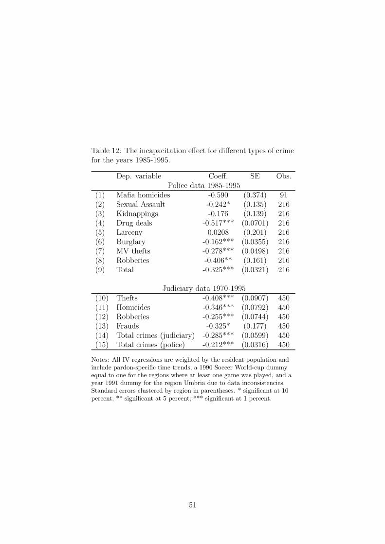
Table 12: The incapacitation effect for different types of crimefor the years 1985-1995.
Dep. variable Coeff. SE Obs.Police data 1985-1995
(1) Mafia homicides -0.590 (0.374) 91(2) Sexual Assault -0.242* (0.135) 216(3) Kidnappings -0.176 (0.139) 216(4) Drug deals -0.517*** (0.0701) 216(5) Larceny 0.0208 (0.201) 216(6) Burglary -0.162*** (0.0355) 216(7) MV thefts -0.278*** (0.0498) 216(8) Robberies -0.406** (0.161) 216(9) Total -0.325*** (0.0321) 216
Judiciary data 1970-1995(10) Thefts -0.408*** (0.0907) 450(11) Homicides -0.346*** (0.0792) 450(12) Robberies -0.255*** (0.0744) 450(13) Frauds -0.325* (0.177) 450(14) Total crimes (judiciary) -0.285*** (0.0599) 450(15) Total crimes (police) -0.212*** (0.0316) 450
Notes: All IV regressions are weighted by the resident population andinclude pardon-specific time trends, a 1990 Soccer World-cup dummyequal to one for the regions where at least one game was played, and ayear 1991 dummy for the region Umbria due to data inconsistencies.Standard errors clustered by region in parentheses. * significant at 10percent; ** significant at 5 percent; *** significant at 1 percent.
51
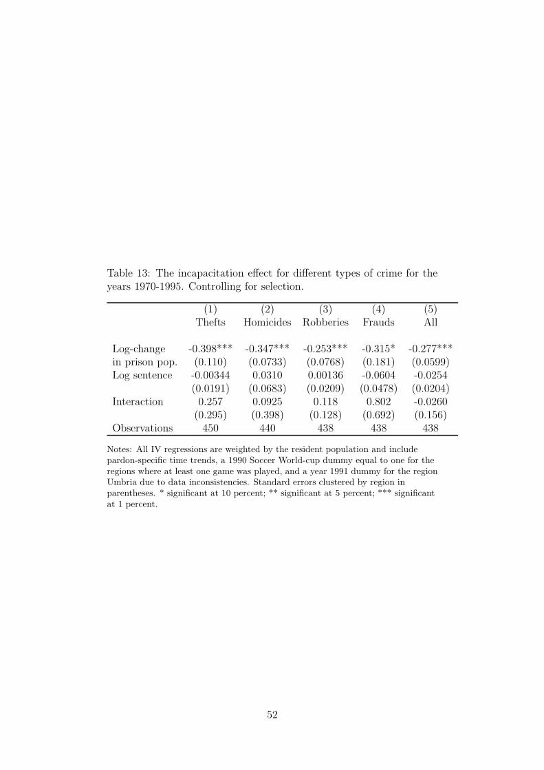
Table 13: The incapacitation effect for different types of crime for theyears 1970-1995. Controlling for selection.
(1) (2) (3) (4) (5)Thefts Homicides Robberies Frauds All
Log-change -0.398*** -0.347*** -0.253*** -0.315* -0.277***in prison pop. (0.110) (0.0733) (0.0768) (0.181) (0.0599)Log sentence -0.00344 0.0310 0.00136 -0.0604 -0.0254
(0.0191) (0.0683) (0.0209) (0.0478) (0.0204)Interaction 0.257 0.0925 0.118 0.802 -0.0260
(0.295) (0.398) (0.128) (0.692) (0.156)Observations 450 440 438 438 438
Notes: All IV regressions are weighted by the resident population and includepardon-specific time trends, a 1990 Soccer World-cup dummy equal to one for theregions where at least one game was played, and a year 1991 dummy for the regionUmbria due to data inconsistencies. Standard errors clustered by region inparentheses. * significant at 10 percent; ** significant at 5 percent; *** significantat 1 percent.
52

Table 14: Social benefit from incarceration
Total Elasticity Reporting prob. Marginal effect Cost per crime Social cost
Against the person
Massacre 24 0? - - - -Mafia related murder 299 0.00 1.00 0.00 0.00 0.00non-Mafia related murder 1,249 0.35 1.00 0.01 2,679,690 21,052Attempted murder 1,542 0.35 1.00 0.01 ? ?Infanticide 6 ? - - - ?Voluntary manslaughter 83 ? - - - ?Involuntary manslaughter 8,294 ? - - - ?Sexual assault 4,571 0.24 1.00 0.02 50,600 1,018Other (including assault, battery, pornography) 290,612 0 ? - - - ?Against the family, the morale, the animals
18,180 0 ? - - - -Against property
Motor vehicle theft (motorbikes) 80,494 0.28 0.95 0.43 2,156 928Motor vehicle theft (cars) 182,470 0.28 0.87 1.07 7,145 7,618Other thefts 1,252,117 0.41 0.54 17.16 326 5,594Bank robbery 2,683 0.41 1.00 0.02 324,809 6,465Other robberies 47,046 0.26 0.50 0.44 38,330 16,856Extorsion 8,024 ? - - - -Kidnappings 196 0.00 - - - -Harm to things, animals, property, etc. 300,352 ? - - - -Fraud 301,428 0.33 1.00 1.78 9,953 17,727Against the economy and the public trust
Commercial fraud 8,583 0.33 1.00 0.05 9,953 505Drug related crimes 33,417 0.52 1.00 0.31 - ?Other (forged currency, counterfeit) 193,095 0.33 1.00 1.14 - ?Against the State and the public order
74,610 0 ? - - - -Other crimes
153,878 0 ? - - - -
Total social cost 77,762.61Total social cost excluding frauds 60,035.34
Notes: See Section 5 for the list of sources and assumptions used.
53