DPRIETI Discussion Paper Series 16-E-020

The Incidence of Health Insurance Costs:Empirical evidence from Japan

HAMAAKI JunyaHosei University

The Research Institute of Economy, Trade and Industryhttp://www.rieti.go.jp/en/

1

RIETI Discussion Paper Series 16-E-020

March 2016

The Incidence of Health Insurance Costs:

Empirical evidence from Japan†

HAMAAKI Junya*

Abstract

Empirical studies on the incidence of social security contributions in Japan have produced

conflicting results. Against this background, the present study, using new panel data, examines the

extent to which employers’ health insurance contributions have been shifted to employees through

the adjustment of wages following a major reform of the way insurance contributions are calculated.

The results indicate that a large part of employers’ contribution burden was shifted to employees,

and that this tendency was particularly pronounced for health insurers with a large number of

insurees. This finding is consistent with the view that the labour supply in Japan is inelastic with

regard to changes in wages. Furthermore, the empirical results suggest that the increase in employers’

insurance burden following the reform was not passed on to employees immediately but rather over

time through the gradual adjustment of wages.

Keywords: Health insurance, Social insurance contributions, Incidence

JEL classification codes: H51, I13, J38

† This study was conducted as a part of the project “Social security system to revive economic vitality and improve the quality of life,” undertaken at Research Institute of Economy, Trade and Industry (RIETI). I am grateful to Masahisa Fujita, Mitsuhiro Fukao, Naomi Miyazato, Tadashi Sakai, Yoko Ibuka, Reo Takaku, Daiji Kawaguchi and Ralph Paprzycki for valuable comments on an earlier draft of this paper. I would also like to thank participants of the 2012 Autumn Meeting of the Japanese Economic Association held at Kyushu Sangyo University and seminar participants at Aoyama Gakuin University, the National Institute of Population and Social Security Research, the Osaka University Nakanoshima Center, Kagoshima University and RIETI for their helpful comments. This work was supported by JSPS KAKENHI Grant Number 25780184 and 24330097. * Associate professor at the Faculty of Economics, Hosei University. Postal Address: 4342 Aihara-machi, Machida-shi, Tokyo 194-0298, Japan. E-mail: hamaaki@hosei.ac.jp.

RIETI Discussion Papers Series aims at widely disseminating research results in the form of professional

papers, thereby stimulating lively discussion. The views expressed in the papers are solely those of the

author(s), and neither represent those of the organization to which the author(s) belong(s) nor the Research

Institute of Economy, Trade and Industry.

2

I. Introduction

As Japan’s population continues to age, a major challenge is how to ensure the financial sustainability

of the health insurance system in the face of rising health care costs. One aspect of this is the growing

mandatory transfers in recent years from other health insurance providers to the National Health

Insurance, which many of the elderly have joined. In order to pay these transfers, these other health

insurance providers, in turn, have been forced to greatly increase their members’ health insurance

contributions. A pertinent question that arises in this context is who ultimately bears the costs of

increased insurance contributions – employers or employees. From an economic perspective, even if

nominally both employers and employees bear the costs of insurance contributions, who ultimately

pays for them may be a different matter.

The question of whether it is ultimately employers or employees that bear the costs of social

insurance contributions, that is, the incidence of insurance contributions, has been the subject of a

considerable number of empirical studies, including in Japan (e.g., Tachibanaki and Yokoyama, 2008;

Komamura and Yamada, 2004; Iwamoto and Hamaaki, 2006, 2009; Sakai, 2006; Sakai and Kazekami,

2007; Hamaaki and Iwamoto, 2010). Initially, the findings of these studies varied greatly, ranging from

Tachibanaki and Yokoyama’s (2008) result that there was no shifting of the social insurance burden to

employees to Komamura and Yamada’s (2004) result that there was almost complete shifting through

lower wages. Iwamoto and Hamaaki (2006, 2009) and Hamaaki and Iwamoto (2010) examined in

detail why these studies arrived at opposite results and argued that the estimates in both studies may

be biased. Overall, however, these studies have given rise to the widespread perception that employers’

contributions are at least partly shifted to employees via lower wages, although there is no consensus

on roughly what share of employers’ contribution is shifted.

Against this background, the purpose of the present paper is to empirically investigate the

extent to which the incidence of health insurance costs in Japan is shifted from employers to employees.

Specifically, employing panel data on health insurance societies (HISs),1 the paper focuses on the

increase in the burden of insurance contributions as a result of the introduction of the total

remuneration system (TRS) in 2003. There are (at least) two advantages to using the introduction of

the TRS, which will be explained in more detail below, for the analysis here. The first is that the TRS

introduction gave rise to large changes in contribution rates, so that it is possible to use for the

empirical analysis not only differences in contribution rates across different HISs but also changes

over time. The second advantage is that by using differences in the extent to which contribution rates

changed in the wake of the TRS introduction, it is possible to examine how wages were adjusted over

time following the TRS introduction. The study by Sakai (2006), in fact, also used the TRS

introduction for analysis. However, because he used aggregate data (data aggregated by workers’

1 Health insurance societies are health insurance providers established by one or a number of firms in the same industry. A detailed outline of Japan’s health insurance system and the role of health insurance societies is provided in the next section.

3

attributes), his estimates greatly differ from the theoretically expected range.

Using more detailed data, the analysis in this study suggests that a large part of the burden

of employers’ insurance contribution is indeed shifted to employees via lower wages. The pattern is

particularly pronounced for HISs with a large number of insurees. This result is consistent with the

fact that the labour supply in Japan is generally considered to be inelastic with regard to wages. It is

also in line with findings for other countries suggesting that a large part of employers’ insurance burden

is shifted to employees, such as Gruber (1997) for Chile, Kugler and Kugler (2009) for Columbia,

Holmlund (1983) for Sweden, Hamermesh (1979) for Britain, and Gruber and Krueger (1991), Gruber

(1994), and Anderson and Meyer (2000) for the United States. Furthermore, the results obtained here

suggest that the increase in employers’ insurance burden through the TRS introduction was not passed

on to employees immediately but rather occurred over time through the gradual adjustment of wages.

The remainder of this study is organized as follows. Section II provides an outline of the

Japanese health insurance system and explains the theoretical framework for the analysis. Next,

Section III describes the data used for the analysis and explains the empirical approach. Section IV

then presents the estimation results and their interpretation, while Section V concludes.

II. Institutional Background and Theoretical Framework

Description of the Japanese health insurance system

Before turning to the estimation approach and data, it may be helpful to provide a brief outline of the

Japanese health insurance system and explain the health insurance societies (HISs) on which the

analysis will focus. Specifically, the description here refers to the system up to 2007, which is what

the analysis in this paper focuses on.2 The system goes back to 1961, when universal health insurance

was first established and all citizens became members of the public health insurance. Broadly speaking,

health insurance was divided into occupation-based and region-based insurance schemes. Occupation-

based insurance schemes include society-managed health insurance plans for employees, which cover

the employees of large corporations and affiliated group companies and the dependents of such

employees; a government-managed health insurance plan, which covers mainly the employees of

small and medium-sized enterprises and their dependents; and mutual aid associations and the

seamen’s insurance, which cover specific employees such as public employees and seamen and their

dependents. Region-based insurance schemes consist of National Health Insurance plans managed by

individual municipalities and National Health Insurance societies established for specific occupations.

2 Japan’s health care insurance system was dramatically overhauled after 2007. For example, since October 2010, government-managed health insurance plans are no longer administered directly by the central government (Social Insurance Agency), but are now managed by a corporation called the Japan Health Insurance Association. Moreover, in 2008, the Health Care Program for the Elderly (HCPE, Rojin-Hoken Seido) became the Latter-Stage Elderly Health Care Program (for those aged 75 and over), and whereas in the past the elderly that had joined the National Health Insurance were automatically also members of the HCPE, the elderly now join the Latter-Stage Elderly Health Care Program separately set up specifically for them.

4

The focus of this study is the society-managed health insurance plans for employees. In 2003,

such plans covered about 30.27 million persons, i.e., about one in four of Japan’s population overall.

During the period this study focuses on, there were approximately 1,600 health insurance societies in

Japan3 set up either by a single firm or jointly by a number of firms in the same industry, each of

which independently determines the insurance contributions it charges and the benefits it provides.

Contributions are set so as to ensure that the finances of an HIS are balanced, and depending on the

HIS, contribution rates for employers and employees together ranged from 3.0% to 9.5% of employees’

income.4 In principle, employers and employees are meant to share the contributions equally, with

each side paying half. However, if an HIS so decides, employers’ share of contributions can exceed

50%.

The HISs pay their various kinds of expenditures from the income they receive in the form

of insurees’ premium contributions (and from subsidies for financially pressed societies from the

government’s general budget). The largest expenditure item is statutory medical benefit payments

consisting of various kinds of medical expenses as well as injury, sickness, childbirth, and maternity

allowances, which together account for about 50% of total expenditures. The second largest item is

contributions to the Health Care Program for the Elderly (HCPE, Rojin-Hoken Seido) and the Health

Care Program for Retired Employees, which account for 35–40% of total expenditures. In recent years,

the spiralling burden of these contributions has led to a deterioration in HISs’ finances.

The Total Remuneration System

The key aim of this paper is to estimate the extent of the shifting of the health care insurance burden

from employers to employees taking advantage of the change in insurance contribution rates as a result

of the introduction of the total remuneration system (TRS). Before the introduction of the TRS,

contribution rates were determined solely on the bases of employees’ monthly wages, excluding

bonuses. However, this gave rise to a situation where employees with the same annual remuneration

would pay different insurance contributions, with those receiving a larger share of their remuneration

in bonuses paying lower insurance contributions. The TRS was introduced in April 2003 to redress

this unfairness by basing contribution rates on employees’ total remuneration, i.e., their monthly

income as well as bonuses. Of course, this meant that nominal contribution rates were lowered in

response to the TRS introduction, giving the impression that the burden of insurance contributions did

not change very much. However, Abe (2006) has argued that in practice the insurance burden for

regular employees increased following the introduction of the TRS.

Theoretical framework

3 Specifically, there were 1,622 HISs in FY2003, but by FY2015, that number had fallen to 1,403. 4 While the upper limit of the total contribution rate for employers and employees during the observation period was 9.5%, this has since risen to 12% and will be raised further to 13% in April 2016.

5

To consider the incidence of social security contributions, it is helpful to look at two alternative cases

depending on the value employees place on the benefits provided by social security. The incidence of

social security contributions is equivalent to the incidence of taxes when employees place no value on

such benefits. That is, whether social security contributions are borne by employers or employees does

not affect the final incidence. Moreover, the incidence of the burden is determined by the wage

elasticity of the demand for and supply of labour.

Next, let us theoretically consider the determination of wages and employment in the labour

market in the case that workers do value social security benefits. Let us assume that labour demand

by employers depends on wage augmented by employers’ social security contributions :

1 (1)

Further, let us assume that labour supply depends on wage less employees’ social security

contributions , as well as the value that employees place on social security benefits:

1 (2)

where is the part of employees’ social security contributions whose benefits they do not value, and

is the part of employers’ social security contributions whose benefits they do value.

The focus of empirical research on social security contribution burdens is the impact of the

employer burden on market wages. In terms of the model specification above, this can be expressed

as follows:

(3)

Equation 3 implies that a 1 percentage point change in the insurance contribution rate leads to an x%

change in wages.

From a theoretical perspective, there are three cases in which employers’ burden fully falls

back on employees by inducing a decline in market wages: (1) when labour supply is perfectly inelastic

( 0 ); (2) when labour demand is perfectly elastic ∞ ; and (3) when the burden of

employees’ social security contributions is exactly the same as the value they place on social security

benefits ( 0， 1 . In all of these cases, Equation 3 reduces to

6

(4)

and employers’ burden is fully shifted to employees via wages, so that it is employees that actually

bear the burden of social security contributions. Previous studies such as Bessho and Hayashi (2005),

Kuroda and Yamamoto (2008) and Bessho (2010) suggest that the labour supply of Japanese workers,

particularly of male workers, appears to be inelastic to wages. Combining this observation with the

fact that, according to the data used in the present study, male workers make up roughly three quarters

of the HISs’ insurees during the observation period (2001 to 2007), suggests that labour supply in

Japan is relatively inelastic. Therefore, Equation 3 likely reduces to Equation 4 for Japan.

III. Data and Empirical Strategy

Data

The analysis in this study uses panel data for HISs from the Financial Statements of Health Insurance

Societies (Kenko-hoken kumiai jigyo nenpo in Japanese) published by the National Federation of

Health Insurance Societies (referred to as Financial Statements below). The Financial Statements

provide information on the number of insurees, their wages, the contribution rates of workers and

employers, etc., for all HISs in Japan. Because the analysis in this study also requires information on

the average age of insurees, the information from the Financial Statements is matched with

information on the average age of insurees by HIS from the Status Report on Health Insurance

Societies (Kenko-hoken kumiai no gensei in Japanese), also published by the National Federation of

Health Insurance Societies. For the analysis, data on the 1,210 HISs for which information throughout

the period from 2001 to 2007 is available in the Financial Statements is used. This number excludes

HISs – about a fifth of all HISs – which already before the introduction of the TRS imposed a “special

insurance premium” on bonuses. The reason for excluding such HISs is that it is not possible to

calculate the change in contribution rates following the TRS introduction, which is used in the analysis

in Section IV.

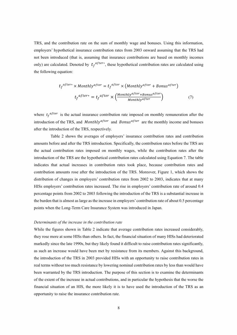
Descriptive statistics of the variables employed in the analysis are shown in Table 1.

Standard monthly remuneration (in real terms, adjusted using the consumer price index) increased

only slightly during the observation period, reflecting sluggish economic growth. At the same time,

employers’ health insurance contribution rate5 decreased, but this is likely the result of the decline in

5 Employers’ contribution rate here does not take employers’ long-term care insurance contributions into account. The reason is that although information on the long-term care insurance contribution rate of each HIS is available, no information is available on the respective shares borne by employers and employees. Nevertheless, to check the robustness of the results, the estimations were repeated assuming that long-term care insurance contributions are split between employers and employees at the same ratio as health insurance contributions. For example, if health insurance contributions in a particular HIS are split equally between employers and employees, the same ratio (i.e., fifty-fifty) was assumed for long-term care insurance contributions. However, the estimation results remained essentially unchanged when including long-term care insurance contributions in this manner.

7

HISs’ contributions to the Health Care Program for the Elderly as the eligible age for the program was

raised by one year every year. Finally, the average age of insurees gradually increased during the

observation period, reflecting the growing share of middle-aged and older employees within firms.

Empirical framework

In order to gauge the extent of the shift of employers’ burden to employees via wages shown by

Equation 3, and following the example of numerous previous empirical studies, the following

specification for the log of wages is estimated:

ln (5)

where is a vector of independent variables other than employers’ contribution rate affecting wages,

and is the error term. Variables included in are the log of the number of insurees, the average

age of insurees, year dummies, industry dummies, interaction terms of the industry dummies and a

trend variable, and two dummies for HISs that are outliers in terms of their insurees’ average wage

(specifically, the dummies identify HISs whose insurees’ average wage falls into the top or bottom

percentile of the distribution of HISs in terms of their insurees’ average wage). The purpose of

including the interaction terms of the industry dummies and a trend variable is to control for different

wage trends across industries. is the parameter of interest showing to what extent employers’

burden is shifted to workers in the form of a decline in wages. If employers’ burden is completely

shifted to workers, will be equal to 1 1⁄ , and if the unit of is %, will be close to -

0.01.

Further, in order to gauge the extent to which employers’ burden is shifted utilizing the

change in contribution rates as a result of the TRS introduction, in addition to Equation 5, the following

equation, which takes the difference of Equation 5 before and after the TRS introduction, is estimated:

ln ⁄ ∆ ∆ (6)

where ∆ includes the rate of change in the number of insurees, the change in the average age of

insurees, industry dummies, and two dummies for HISs that are outliers in terms of their insurees’

average wage.

In order to estimate Equation 6, it is necessary to calculate ∆ , the change in contribution

rates following the TRS introduction, from the HIS panel data constructed from the Financial

Statements. Information available from the Financial Statements includes the average monthly wage

of insurees at a particular HIS before the introduction of the total remuneration system as well as the

contribution rate on that wage, the monthly wage and bonus payments after the introduction of the

8

TRS, and the contribution rate on the sum of monthly wage and bonuses. Using this information,

employers’ hypothetical insurance contribution rates from 2003 onward assuming that the TRS had

not been introduced (that is, assuming that insurance contributions are based on monthly incomes

only) are calculated. Denoted by ∗, these hypothetical contribution rates are calculated using

the following equation:

∗

∗ (7)

where is the actual insurance contribution rate imposed on monthly remuneration after the

introduction of the TRS, and and are the monthly income and bonuses

after the introduction of the TRS, respectively.

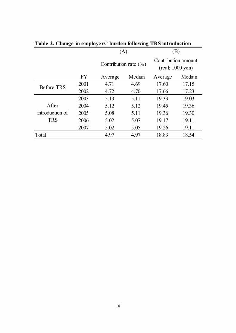
Table 2 shows the averages of employers’ insurance contribution rates and contribution

amounts before and after the TRS introduction. Specifically, the contribution rates before the TRS are

the actual contribution rates imposed on monthly wages, while the contribution rates after the

introduction of the TRS are the hypothetical contribution rates calculated using Equation 7. The table

indicates that actual increases in contribution rates took place, because contribution rates and

contribution amounts rose after the introduction of the TRS. Moreover, Figure 1, which shows the

distribution of changes in employers’ contribution rates from 2002 to 2003, indicates that at many

HISs employers’ contribution rates increased. The rise in employers’ contribution rate of around 0.4

percentage points from 2002 to 2003 following the introduction of the TRS is a substantial increase in

the burden that is almost as large as the increase in employers’ contribution rate of about 0.5 percentage

points when the Long-Term Care Insurance System was introduced in Japan.

Determinants of the increase in the contribution rate

While the figures shown in Table 2 indicate that average contribution rates increased considerably,

they rose more at some HISs than others. In fact, the financial situation of many HISs had deteriorated

markedly since the late 1990s, but they likely found it difficult to raise contribution rates significantly,

as such an increase would have been met by resistance from its members. Against this background,

the introduction of the TRS in 2003 provided HISs with an opportunity to raise contribution rates in

real terms without too much resistance by lowering nominal contribution rates by less than would have

been warranted by the TRS introduction. The purpose of this section is to examine the determinants

of the extent of the increase in actual contributions, and in particular the hypothesis that the worse the

financial situation of an HIS, the more likely it is to have used the introduction of the TRS as an

opportunity to raise the insurance contribution rate.

9

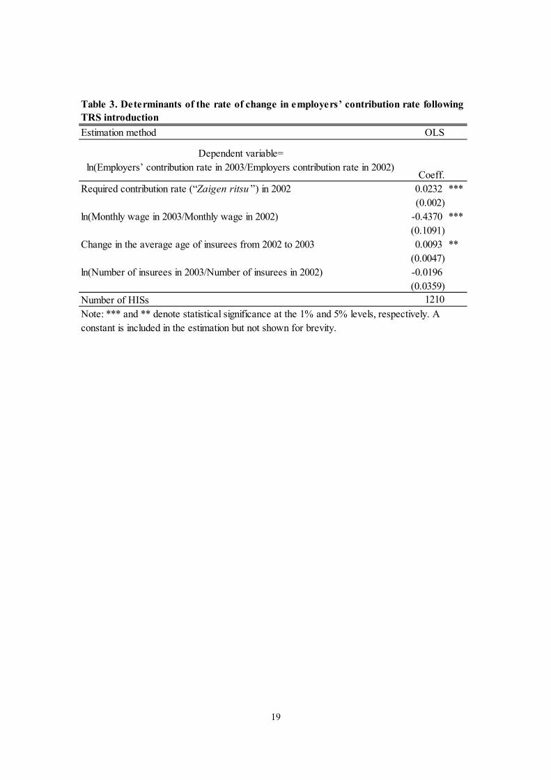
The hypothesis is examined by regressing the change in contribution rates after the TRS

introduction on HISs’ financial situation and other characteristics. As a proxy for HISs’ financial

situation, the contribution rate necessary to make statutory benefit and other payments, which is

referred to as “Zaigen ritsu” in Japanese, is used. This is the contribution rate an HIS needs to cover

mandatory expenses such as statutory benefit payments and contributions to the Health Care Program

for the Elderly and the Health Care Program for Retired Employees. The rate is calculated by dividing

an HIS’s mandatory expenses by the total amount of remunerations on which health insurance

contributions are imposed. This rate will be referred to as the “required contribution rate” hereafter,

and the higher this rate is, the worse is the financial situation of an HIS.6 The results of regressing the

change in the contribution rate from 2002 to 2003 on the required contribution rate and a range of

other variables are shown in Table 3 and indicate that the coefficients on the required contribution rate

in 2002, as well as the rate of change in members’ monthly wages and the change in the average age

of insurees are all significant. This result suggests that the worse the financial situation of an HIS was

before the introduction of the TRS, the more it subsequently raised employers’ contribution rate.

A further notable result in Table 3 is the significantly negative coefficient on the rate of

change in monthly wages following the TRS introduction, which gives rise to the concern that the

extent of shifting may be overestimated when using Equation 6 as a result of reverse causality from

the rate of change in members’ monthly wages to the rate of change in the contribution rate. There are

two possible factors that may give rise to such reverse causality. One is that HISs whose insurees

enjoyed large wage increases were able to raise the funds they needed while restraining increases in

contribution rates. Another is that even though total remuneration may have remained unchanged, the

relative weight of monthly wages and bonuses following the TRS introduction may have changed,

giving rise to a negative correlation between monthly wages and the contribution rate. In other words,

in terms of Equation 7, and assuming that total remuneration remained unchanged, an increase in the

weight of monthly wages would be associated with higher monthly wages and a decrease in the

contribution rate. A potential concern therefore is that a change in the weight of monthly wages in total

remuneration may result in overestimating the extent of shifting.

In order to deal with any potential endogeneity of the change in the contribution rate, in the

analysis below the required contribution rate before the TRS introduction is used as an instrumental

variable when estimating Equation 6.7 There are a number of reasons why the required contribution

6 This is the rate on which the Ministry of Health, Labour and Welfare bases its guidance to HISs with regard to their financial consolidation. 7 It should be noted that instead of the required contribution rate for 2002 that for 2001 is used as the instrument. The reason for using the required contribution rate for 2001 is that this avoids any potential correlation between the instrument and the error term in Equation 6 (i.e., ). For example, if there was a temporary positive shock to wages in the year 2002, HISs’ financial situation would improve through an increase in revenue. As a result, the required contribution rate would fall, because the denominator, i.e., the total amount of monthly remunerations, would increase. Therefore, would be positively correlated with the required contribution rate in 2002.

10

rate makes a good instrument. First, the financial situation of an HIS satisfies the assumption of

instrument relevance. As seen in the regression results in Table 3, the worse the financial situation of

an HIS prior to the TRS introduction, the larger the increase in the contribution rate following the TRS

introduction tended to be. Second, HISs’ financial situation prior to the TRS introduction can be treated

as an exogenous variable. HISs’ financial situation is pre-determined when the monthly wages of

individual HISs’ insurees are set following the TRS introduction. Moreover, it is difficult for HISs to

control their financial situation, because this is greatly affected by fluctuations in the contributions

they have to make to the Health Care Program for the Elderly and the Health Care Program for Retired

Employees. Although these account for a large share of HISs’ expenses – almost 40% – they are

calculated based on variables over which the HISs have no control.8

IV. Estimation Results

Estimation not using the TRS introduction

To start with, Equation 5 is estimated without using the TRS introduction. First, the estimation uses

total monthly remunerations, that is, the standard monthly remuneration plus bonuses/12, as the

dependent variable. The estimation here focuses on the period from 2003 to 2007, that is, excluding

the substantial change in contribution rates (as a result of the TRS introduction) between 2002 and

2003. The estimation results are shown in Table 4, with Columns A to C presenting the results obtained

using a pooled OLS, random effects, and fixed effects model, respectively. The results of the Breusch-

Pagan and Hausman tests suggest that the fixed effects model is the preferred model. In the fixed

effects estimation in Column C, the coefficient on employers’ contribution rate is -0.011, indicating

that employers’ burden was shifted in its entirety to employees via wages.

Next, in order to examine whether employers’ burden was shifted to the standard monthly

remuneration or bonuses, additional regressions are run using each of the two variables as the

dependent variable. The results are shown in Table 5. Focusing again on the results of the fixed effects

model (Columns C and F), the coefficient on employers’ contribution rate is -0.0037 when the standard

monthly remuneration is the dependent variable and -0.0524 when bonuses are the dependent variable.

Using the share of the standard monthly remuneration and bonuses in total remuneration, these

coefficients can be converted into values presenting the extent to which employers’ insurance

contributions were shifted to employees through a decrease in the standard monthly remuneration

and/or bonuses.9 These converted values, which, as shown in Columns C and F, are -0.0030 and -

8 Contributions to the Health Care Program for the Elderly are calculated as the product of each HIS’s health care expenses per elderly person, each HIS’s number of members, and a number of variables common to all HISs. Thus, although each HIS has an incentive to restrain health care expenses per elderly person to reduce contributions and hence its financial burden, this, as Abe (2007) shows, does not necessarily mean that health care expenses on the elderly are indeed significantly reduced. Therefore, contributions to the Health Care Program for the Elderly are not something that individual HISs can control directly. 9 For example, multiplying the coefficient on employers’ contribution rate, presented in Column C of Table 5, by the share of the monthly remuneration in total remuneration yields the extent to which employers’ insurance contributions

11

0.0106 respectively suggest that a large fraction of employers’ burden was shifted through a decrease

in bonuses. Although the coefficient on employers’ contribution rate may be negatively biased due to

the abovementioned endogeneity, this inference is still valid as long as the bias is of a similar size in

both estimations, i.e., that for the monthly remuneration and that for bonuses.

Let us compare the results with those obtained by Komamura and Yamada (2004) and

Iwamoto and Hamaaki (2006, 2009), who conducted similar estimations using the same data (albeit

for different observation periods from the one used here). Comparing the result in Column C in Table

5 with the coefficient estimates for employers’ contribution rate of -0.009 in Komamura and Yamada

(2004) and Iwamoto and Hamaaki (2006, 2009), the absolute value of the coefficient in the present

study is quite small. A possible reason is that the observation period in this study is more recent than

that in Komamura and Yamada (2004) and Iwamoto and Hamaaki (2006, 2009) and is a period in

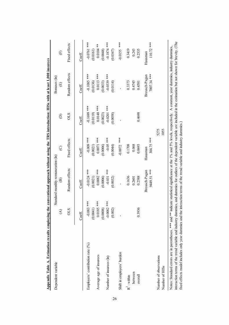
which the proportion of HISs with relatively few insurees increased.10 In fact, when including only

HISs with at least 1,000 insurees in the estimation, the coefficient estimate for employers’ contribution

rate in the fixed effects model becomes -0.009 (see Appendix Table A), which is exactly the same

value as that obtained in the other studies. At HISs that are so small that the law of large numbers does

not work, annual changes in health care expenditure per person tend to be relatively large, so that

changes in contribution rates are also large. However, assuming that it takes time for employers to

shift contributions to employees, changes in contribution rates and wages at such small HISs are

probably “out of sync,” so that it is likely difficult to obtain significant estimates of a stable relationship

between wages and contribution rates.

Estimation using the TRS introduction

Next, the wage function using the change in contribution rates as a result of the TRS introduction is

estimated.11 In order to estimate Equation 6, it is necessary to take the difference of all variables. To

do so, 2002 is taken as the point in time before the TRS introduction and the years from 2003 to 2007

as the time after the TRS introduction. Moreover, although Table 1 suggested that, on average, monthly

wages did not change much following the introduction of the TRS, there are some HISs at which

insurees’ monthly wages did change by 10% or more. Thus, to deal with such outliers, the dummies

were shifted to employees through a decrease in the monthly remuneration. 10 As seen in Table 1, the average number of insurees gradually increased during the observation period. The median number of insurees, however, decreased from 3,925.5 (in 2001) to 3,858.5 (in 2007). Further, the proportion of HISs with 1,000 or fewer insurees, for example, increased from 9.4% (in 2001) to 11.7% (in 2007). 11 Using the actual contribution rate before the TRS introduction and the (hypothetical) contribution rate after the TRS introduction, ∗, as employers’ contribution rate, Equation 5 can also be estimated for the whole observation period 2001–2007 instead of for the period 2003–2007, i.e., the period after the TRS introduction. The results of this estimation are shown in Appendix Table B. The coefficient on the contribution rate in Column C is -0.0093. Compared to the coefficient estimate obtained for the period 2003–2007 (shown in Column C of Table 5), the coefficient is much larger (in absolute value). Due to the increase in the sample size, the estimate might be close to the population value. Another possible explanation for this change is that including the years 2001 and 2002 results in a more accurate estimation of the relationship between wages and contribution rates, since these years include more large-scale HISs than the years after 2002.

12

for HISs falling into the top or bottom percentile of HIS observations in terms of the rate of change in

insurees’ monthly wages are added for the estimation as control variables. Furthermore, the average

age of insurees is also added to Equation 6 in order to purge any correlation between the instrument,

i.e., the required contribution rate, and the error term. In HISs whose average age of insurees is high,

the rate of change of the standard monthly remuneration, i.e., the dependent variable in Equation 6, is

likely to be low. At the same time, the financial situation of such HISs is likely to be worse; that is,

the required contribution rate is likely to be large. Therefore, if the average age is omitted from the

equation, the coefficient on the change of employers’ contribution rate will potentially be negatively

biased due to the correlation between the omitted age variable and the instrument.

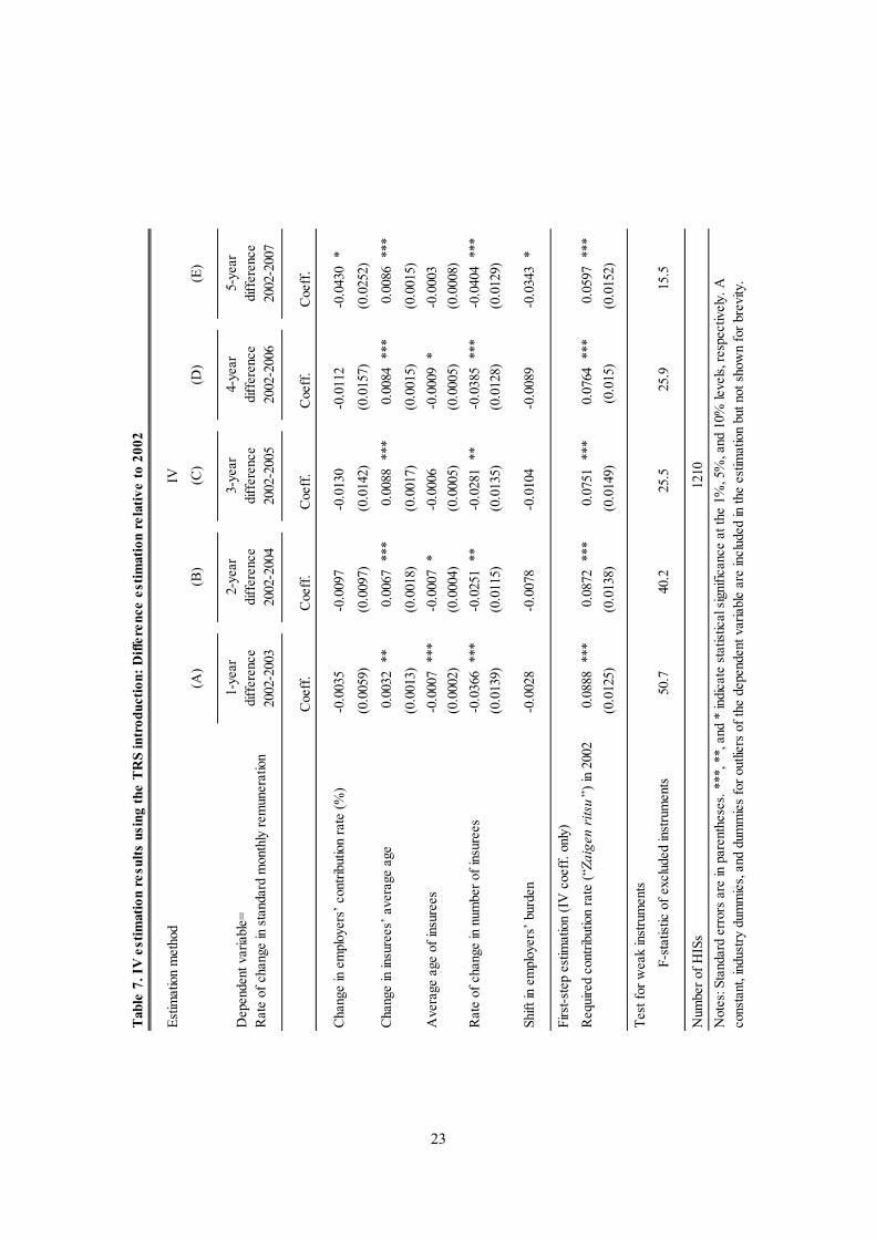
Tables 6 and 7 show the estimation results for Equation 6 using OLS and instrumental

variable (IV) models, respectively. Both in the OLS and IV estimations, the coefficients on employers’

contribution rate are negative, but insignificant, except for Column E. In fact, the finding that the

coefficients are insignificant does not seem implausible given that the dependent variable of the

estimation does not include bonuses, which, as seen above, bore the brunt of the shift of the

contribution burden from employers to employees. If bonuses were also taken into account, the

shifting of the health insurance burden to employees would be found to be significant.12 Moreover,

regardless of the estimation method, the longer the timespan over which the difference is taken, the

larger the extent of the shifting tends to gradually become. This result suggests that the increase in

employers’ burden as a result of the TRS introduction was not immediately shifted to employees, but

was shifted slowly over time through the gradual adjustment of wages. The OLS estimation results

suggest that in the year immediately after the TRS introduction, none of the increase in employers’

contributions had been shifted to employees via the monthly remuneration (Column A), but by 5 years

after the TRS introduction, 50% of the increase had been shifted (Column E). This gradual adjustment

of wages over time may be due to the low inflation rate during the observation period. If the inflation

rate is high, employers can easily reduce real wages without reducing nominal wages. Under low

inflation (or deflation), however, since downward nominal wage rigidity constrains the flexible

adjustment of real wages, it is difficult for employers to cut real wages immediately after an increase

in their contribution rate.

Finally, it is necessary to consider why the absolute values of the coefficients in the IV

estimation in Table 7 are larger than the corresponding coefficients in the OLS estimation in Table 6.

If the coefficient estimates for employers’ contribution rate in Table 6 were indeed biased as a result

of an increase in the weight of monthly wages in total remuneration following the TRS introduction

12 The Financial Statements do not include information on bonuses for 2001 and 2002, although such information is available for the period 2003-2007. Therefore, it is not possible in this study to use the rate of change in total monthly remuneration (or bonuses only) between before and after the introduction of the TRS as the dependent variable in Equation 6, so that it can only be conjectured – rather than empirically verified – that the health insurance burden was shifted to employees through a decrease in bonuses.

13

and/or reverse causality from changes in wages to changes in contribution rates, the absolute value of

the coefficient on employers’ contribution rate should become smaller when using IV estimation to

deal with this endogeneity. However, the absolute values of the coefficients in the IV estimation in

Table 7 are larger than the coefficients in the corresponding columns in the OLS estimation in Table

6. One possible explanation, as mentioned in the previous subsection, is that HISs with relatively few

insurees are included in the estimations, so that it is likely difficult to obtain a stable relationship

between changes in wages and changes in contribution rates. Therefore, to observe a stable

relationship, it may be necessary to focus on HISs with a large number of insurees. Tables 8 and 9

show the estimation results using Equation 6 and focusing on HISs with at least 1,000 insurees. While

some of the absolute values of the coefficients in the IV estimations (Columns B and E) are still larger

than those in the OLS estimation, the other IV coefficients become smaller (in absolute value) than

the OLS coefficients.

V. Conclusion

Using panel data from the Financial Statements of Health Insurance Societies, this study empirically

examined the incidence of social security contributions in Japan by focusing on the shifting of

employers’ contributions to employees in the wake of the introduction of the total remuneration system

for the calculation of health care insurance contributions. The results suggest that a large part (if not

all) of employers’ burden was shifted to employees via wages, especially bonuses. The finding is

consistent with the view that labour supply in Japan is inelastic with regard to changes in wages.

Furthermore, the analysis suggested that the increase in employers’ burden as a result of the

introduction of the total remuneration system was not shifted to employees immediately, but instead

was shifted gradually through the adjustment of wages over time. The results of this study thus imply

that although employers’ burden appears to be shifted to employees over time, it may be borne by

employers at least in the short term, particularly under deflation. Policy makers should carefully

consider this mechanism in order to alleviate the potential adverse effect of employers’ insurance

burden on the Japanese economy.

14

References

Abe, Y. (2006) A note on changes in social insurance contribution structure after 2003 (sic) [Sohoshu-

sei to nenkin hokenryo futan: koyo-keitai betsu no bunseki], JCER Economic Journal [Nihon Keizai

Kenkyu], 54, 126–36 (in Japanese).

Abe, Y. (2007) The effectiveness of financial incentives in controlling the health care expenditures of

seniors, Japan and the World Economy, 19, 461–82.

Anderson, P. M. and B. D. Meyer (2000) The effects of the unemployment insurance payroll tax on

wages, employment, claims and denials, Journal of Public Economics, 78, 81–106.

Bessho, S. (2010) Taxation and labour supply [Zei-futan to rodo-kyokyu], Japanese Journal of Labour

Studies [Nihon Rodo Kenkyu Zasshi] 605, 4–17 (in Japanese).

Bessho, S. and M. Hayashi (2005) Economic studies of taxation in Japan: the case of personal

income taxes, Journal of Asian Economics 16, 956–72.

Gruber, J. (1994) The incidence of mandated maternity benefits, American Economic Review, 84, 622–

41.

Gruber, J. (1997) The incidence of payroll taxation: evidence from Chile, Journal of Labor Economics,

15, 72–101.

Gruber, J. and A. B. Krueger (1991) The incidence of mandated employer-provided insurance: lessons

from workers’ compensation insurance, in Tax Policy and the Economy, Vol. 5, D. Bradford (ed.), MIT

Press, 111–43.

Hamaaki, J. and Y. Iwamoto (2010) A reappraisal of the incidence of employer contributions to social

security in Japan, Japanese Economic Review, 61, 427–41.

Hamermesh, D. S. (1979) New estimates of the incidence of payroll tax, Southern Economic Journal,

45, 1208–19.

Holmlund, B. (1983) Payroll taxes and wage inflation: the Swedish experience, Scandinavian Journal

of Economics, 85, 1–15.

15

Iwamoto, Y. and J. Hamaaki (2006) On the incidence of social insurance contributions in Japan: an

economic perspective [Shakai hokenryo no kichaku bunseki], The Quarterly of Social Security

Research [Kikan Shakai-hosho Kenkyu], 42, 204–18 (in Japanese).

Iwamoto, Y. and J. Hamaaki (2009) On the incidence of social insurance contributions in Japan [Shakai

hokenryo no kichaku bunseki], in Empirical Studies on the Financing of Social Security [Shakai-hosho

Zaigen no Koka Bunseki], National Institute of Population and Social Security Research, University

of Tokyo Press, Tokyo, 37–61 (in Japanese).

Komamura, K. and A. Yamada (2004) Who bears the burden of social insurance? Evidence from

Japanese health and long-term care insurance data, Journal of the Japanese and International

Economies, 18, 565–81.

Kugler, A. and M. Kugler (2009) Labor market effects of payroll taxes in developing countries:

evidence from Colombia, Economic Development and Cultural Change, 57, 335–58.

Kuroda, S. and I. Yamamoto (2008) Estimating Frisch labor supply elasticity in Japan, Journal of the

Japanese and International Economies, 22, 566–85.

Sakai, T. (2006) The various impacts of payroll tax on firms’ personnel managements [Shakai hoken

no jigyonushi-futan ga kigyo no koyo-senryaku ni ataeru samazama-na eikyo] The Quarterly of Social

Security Research [Kikan Shakai-hosho Kenkyu], 42, 235–48 (in Japanese).

Sakai, T. and S. Kazekami (2007) Empirical study on incidence of long-term care insurance (sic)

[Kaigo-hoken seido no kichaku bunseki], Journal of Health Care and Society [Iryo to Shakai], 16,

285–301 (in Japanese).

Tachibanaki, T. and Y. Yokoyama (2008) The estimation of the incidence of employer contributions

to social security in Japan, Japanese Economic Review, 59, 75–83.

16

0.2

.4.6

.81

Den

sity

-2 -1 0 1 2 3Changes in employers' contribution rates from 2002 to 2003 (percentage points)

Figure 1. Distribution of changes in employers' contribution rates

17

Tab

le 1

. Des

crip

tive

sta

tist

ics

Fina

ncia

l yea

r20

0120

0220

0320

0420

0520

0620

07

Stan

dard

mon

thly

rem

uner

atio

n (r

eal;

1000

yen

)37

2.41

373.

1937

5.76

379.

3338

1.79

381.

4438

2.00

(69.

77)

(70.

61)

(73.

88)

(77.

02)

(78.

44)

(78.

2)(8

2.18

)E

mpl

oyer

s’ c

ontr

ibut

ion

rate

(%

)4.

713

4.72

24.

113

4.08

74.

040

3.99

63.

993

(0.6

00)

(0.6

09)

(0.6

32)

(0.6

38)

(0.6

17)

(0.6

05)

(0.5

96)

Ave

rage

age

of

insu

rees

40.3

40.5

40.7

40.9

41.0

41.2

41.3

(3.3

77)

(3.3

39)

(3.2

88)

(3.2

16)

(3.1

98)

(3.2

15)

(3.1

72)

Num

ber

of in

sure

es96

1295

0694

4595

1797

1810

023

1033

4(1

8274

)(1

8242

)(1

8360

)(1

8750

)(1

9446

)(2

0547

)(2

1661

)In

dust

ry d

umm

ies

C

hem

ical

indu

stry

0.10

50.

105

0.10

60.

107

0.10

70.

107

0.10

7

Cer

amic

s, s

tone

and

cla

y in

dust

ries

0.01

60.

016

0.01

60.

016

0.01

60.

016

0.01

6

Tex

tile

indu

stry

0.02

10.

021

0.02

00.

019

0.01

90.

019

0.01

9

Mac

hine

ry a

nd a

ppar

atus

indu

strie

s0.

226

0.22

60.

226

0.22

50.

224

0.22

40.

224

O

ther

man

ufac

turin

g0.

082

0.08

30.

083

0.08

20.

082

0.08

20.

082

M

etal

min

ing

indu

stry

0.00

20.

002

0.00

20.

002

0.00

20.

002

0.00

2

Tra

nspo

rtat

ion

busi

ness

0.05

80.

058

0.05

80.

058

0.05

80.

058

0.05

8

Who

lesa

le a

nd r

etai

l tra

de0.

152

0.15

00.

150

0.15

00.

150

0.15

00.

150

F

inan

ce a

nd in

sura

nce

busi

ness

0.12

70.

127

0.12

70.

127

0.12

70.

127

0.12

7

Oth

er b

usin

ess

0.16

10.

162

0.16

20.

164

0.16

40.

164

0.16

4

Off

ices

of

corp

orat

ions

or

orga

niza

tions

0.05

10.

051

0.05

10.

051

0.05

10.

051

0.05

1N

umbe

r of

HIS

s12

10

Not

e: S

tand

ard

devi

atio

ns a

re in

par

enth

eses

.

18

FY Average Median Average Median2001 4.71 4.69 17.60 17.152002 4.72 4.70 17.66 17.232003 5.13 5.11 19.33 19.032004 5.12 5.12 19.45 19.362005 5.08 5.11 19.36 19.302006 5.02 5.07 19.17 19.112007 5.02 5.05 19.26 19.11

Total 4.97 4.97 18.83 18.54

Table 2. Change in employers’ burden following TRS introduction

Afterintroduction of

TRS

(A) (B)

Contribution rate (%)Contribution amount

(real; 1000 yen)

Before TRS

19

Estimation method

Coeff.Required contribution rate (“Zaigen ritsu ”) in 2002 0.0232 ***

(0.002)ln(Monthly wage in 2003/Monthly wage in 2002) -0.4370 ***

(0.1091)Change in the average age of insurees from 2002 to 2003 0.0093 **

(0.0047)ln(Number of insurees in 2003/Number of insurees in 2002) -0.0196

(0.0359)Number of HISs

Table 3. Determinants of the rate of change in employers’ contribution rate followingTRS introduction

OLS

Dependent variable=ln(Employers’ contribution rate in 2003/Employers contribution rate in 2002)

1210

Note: *** and ** denote statistical significance at the 1% and 5% levels, respectively. Aconstant is included in the estimation but not shown for brevity.

20

Table 4. Estimation results employing conventional approach without using TRS introduction

Dependent variable

Coeff. Coeff. Coeff.

Employers’ contribution rate (%) -0.0874 *** -0.0156 *** -0.011 ***(0.0045) (0.0025) (0.0025)

Average age of insurees 0.016 *** 0.0072 *** 0.0058 ***(0.0009) (0.0007) (0.0008)

Number of insurees (ln) -0.0006 -0.0343 *** -0.0856 ***(0.002) (0.0034) (0.0052)

R2

: within 0.1708 0.1929

between 0.1995 0.0124 overall 0.339 0.1988 0.0137

Breusch-Pagan Hausman10636.39 *** 411.07 ***

Number of observationsNumber of HISs 1210

Notes: Standard errors are in parentheses. *** indicates statistical significance at the 1% level. Aconstant, year dummies, industry dummies, interaction terms of the trend variable and industrydummies, and dummies for outliers of the dependent variable are included in the estimation but notshown for brevity. (The fixed effects model includes only year dummies and the interaction terms ofthe trend variable and industry dummies.)

OLS Random effects Fixed effects

Standard monthly remuneration + Bonuses/12 (ln)(A) (B) (C)

6050

21

Tab

le 5

. Est

imat

ion

resu

lts

empl

oyin

g th

e co

nven

tion

al a

ppro

ach

wit

hout

usi

ng t

he T

RS

intr

oduc

tion

Dep

ende

nt v

aria

ble

Coe

ff.

Coe

ff.

Coe

ff.

Coe

ff.

Coe

ff.

Coe

ff.

Em

ploy

ers’

con

trib

utio

n ra

te (

%)

-0.0

749

***

-0.0

069

***

-0.0

037

**-0

.159

***

-0.0

876

***

-0.0

524

***

(0.0

037)

(0.0

019)

(0.0

019)

(0.0

112)

(0.0

126)

(0.0

148)

Ave

rage

age

of

insu

rees

0.01

68**

*0.

0076

***

0.00

65**

*0.

0112

***

0.00

68**

0.00

63(0

.000

7)(0

.000

6)(0

.000

6)(0

.002

2)(0

.003

1)(0

.004

5)N

umbe

r of

insu

rees

(ln

)-0

.001

5-0

.029

2**

*-0

.063

2**

*0.

0038

-0.0

115

-0.1

843

***

(0.0

016)

(0.0

027)

(0.0

039)

(0.0

049)

(0.0

096)

(0.0

306)

Shift

in e

mpl

oyer

s’ b

urde

n -

--0

.003

0**

*-

--0

.010

6**

*

R2

: with

in0.

1587

0.17

850.

4189

0.42

32

betw

een

0.19

930.

0254

0.46

010.

1793

over

all

0.36

760.

1986

0.02

660.

4633

0.45

20.

2089

Bre

usch

-Pag

anH

ausm

anB

reus

ch-P

agan

Hau

sman

1079

2.4

***

455.

33**

*78

39.9

4**

*12

5.72

***

Num

ber

of o

bser

vatio

nsN

umbe

r of

HIS

s

Stan

dard

mon

thly

rem

uner

atio

n (ln

)B

onus

es (

ln)

(A)

(B)

(C)

(D)

(E)

(F)

Fixe

d ef

fect

s

6050

1210

Not

es: S

tand

ard

erro

rs a

re in

par

enth

eses

. ***

and

**

indi

cate

sta

tistic

al s

igni

fican

ce a

t the

1%

and

5%

leve

ls, r

espe

ctiv

ely.

A c

onst

ant,

year

dum

mie

s, in

dust

ry d

umm

ies,

inte

ract

ion

term

s of

the

tren

d va

riabl

e an

d in

dust

ry d

umm

ies,

and

dum

mie

s fo

r ou

tlier

s of

the

depe

nden

t var

iabl

e ar

e in

clud

ed in

the

estim

atio

n bu

t not

sho

wn

for

brev

ity. (

The

fixed

eff

ects

mod

el in

clud

es o

nly

year

dum

mie

s an

d th

e in

tera

ctio

n te

rms

of th

e tr

end

varia

ble

and

indu

stry

dum

mie

s.)

OL

SR

ando

m e

ffec

tsFi

xed

effe

cts

OL

SR

ando

m e

ffec

ts

22

Tab

le 6

. OL

S es

tim

atio

n re

sult

s us

ing

the

TR

S in

trod

ucti

on:

Diff

eren

ce e

stim

atio

n re

lati

ve t

o 20

02

Est

imat

ion

met

hod

Dep

ende

nt v

aria

ble=

Rat

e of

cha

nge

in s

tand

ard

mon

thly

rem

uner

atio

n

Coe

ff.

Coe

ff.

Coe

ff.

Coe

ff.

Coe

ff.

Cha

nge

in e

mpl

oyer

s’ c

ontr

ibut

ion

rate

(%

)-0

.000

5-0

.003

3-0

.004

2-0

.004

0-0

.006

3*

(0.0

014)

(0.0

024)

(0.0

028)

(0.0

033)

(0.0

034)

Cha

nge

in in

sure

es’

aver

age

age

0.00

31**

0.00

67**

*0.

0092

***

0.00

86**

*0.

0095

***

(0.0

013)

(0.0

018)

(0.0

015)

(0.0

014)

(0.0

013)

Ave

rage

age

of

insu

rees

-0.0

008

***

-0.0

008

**-0

.000

7*

-0.0

010

**-0

.001

0*

(0.0

002)

(0.0

003)

(0.0

004)

(0.0

005)

(0.0

006)

Rat

e of

cha

nge

in n

umbe

r of

insu

rees

-0.0

360

***

-0.0

238

**-0

.026

3**

-0.0

370

***

-0.0

366

***

(0.0

134)

(0.0

112)

(0.0

127)

(0.0

118)

(0.0

116)

Shift

in e

mpl

oyer

s’ b

urde

n -0

.000

4-0

.002

7-0

.003

4-0

.003

2-0

.005

0*

Num

ber

of H

ISs

OL

S

(A)

(B)

(C)

(D)

(E)

Not

es: S

tand

ard

erro

rs a

re in

par

enth

eses

. ***

, **,

and

* in

dica

te s

tatis

tical

sig

nific

ance

at t

he 1

%, 5

%, a

nd 1

0% le

vels

, res

pect

ivel

y. A

cons

tant

, ind

ustr

y du

mm

ies,

and

dum

mie

s fo

r ou

tlier

s of

the

depe

nden

t var

iabl

e ar

e in

clud

ed in

the

estim

atio

n bu

t not

sho

wn

for

brev

ity.

1-ye

ardi

ffer

ence

2002

-200

3

2-ye

ardi

ffer

ence

2002

-200

4

3-ye

ardi

ffer

ence

2002

-200

5

4-ye

ardi

ffer

ence

2002

-200

6

5-ye

ardi

ffer

ence

2002

-200

7

1210

23

Tab

le 7

. IV

est

imat

ion

resu

lts

usin

g th

e T

RS

intr

oduc

tion

: D

iffer

ence

est

imat

ion

rela

tive

to

2002

Est

imat

ion

met

hod

Dep

ende

nt v

aria

ble=

Rat

e of

cha

nge

in s

tand

ard

mon

thly

rem

uner

atio

n

Coe

ff.

Coe

ff.

Coe

ff.

Coe

ff.

Coe

ff.

Cha

nge

in e

mpl

oyer

s’ c

ontr

ibut

ion

rate

(%

)-0

.003

5-0

.009

7-0

.013

0-0

.011

2-0

.043

0*

(0.0

059)

(0.0

097)

(0.0

142)

(0.0

157)

(0.0

252)

Cha

nge

in in

sure

es’

aver

age

age

0.00

32**

0.00

67**

*0.

0088

***

0.00

84**

*0.

0086

***

(0.0

013)

(0.0

018)

(0.0

017)

(0.0

015)

(0.0

015)

Ave

rage

age

of

insu

rees

-0.0

007

***

-0.0

007

*-0

.000

6-0

.000

9*

-0.0

003

(0.0

002)

(0.0

004)

(0.0

005)

(0.0

005)

(0.0

008)

Rat

e of

cha

nge

in n

umbe

r of

insu

rees

-0.0

366

***

-0.0

251

**-0

.028

1**

-0.0

385

***

-0.0

404

***

(0.0

139)

(0.0

115)

(0.0

135)

(0.0

128)

(0.0

129)

Shift

in e

mpl

oyer

s’ b

urde

n -0

.002

8-0

.007

8-0

.010

4-0

.008

9-0

.034

3*

Firs

t-st

ep e

stim

atio

n (I

V c

oeff

. onl

y)

Req

uire

d co

ntrib

utio

n ra

te (

“Zai

gen

rits

u”)

in 2

002

0.08

88**

*0.

0872

***

0.07

51**

*0.

0764

***

0.05

97**

*

(0.0

125)

(0.0

138)

(0.0

149)

(0.0

15)

(0.0

152)

Tes

t for

wea

k in

stru

men

ts

　　

　　

F-st

atis

tic o

f ex

clud

ed in

stru

men

ts50

.740

.225

.525

.915

.5

Num

ber

of H

ISs

IV

(A)

(B)

(C)

(D)

(E)

Not

es: S

tand

ard

erro

rs a

re in

par

enth

eses

. ***

, **,

and

* in

dica

te s

tatis

tical

sig

nific

ance

at t

he 1

%, 5

%, a

nd 1

0% le

vels

, res

pect

ivel

y. A

cons

tant

, ind

ustr

y du

mm

ies,

and

dum

mie

s fo

r ou

tlier

s of

the

depe

nden

t var

iabl

e ar

e in

clud

ed in

the

estim

atio

n bu

t not

sho

wn

for

brev

ity.

1-ye

ardi

ffer

ence

2002

-200

3

2-ye

ardi

ffer

ence

2002

-200

4

3-ye

ardi

ffer

ence

2002

-200

5

4-ye

ardi

ffer

ence

2002

-200

6

5-ye

ardi

ffer

ence

2002

-200

7

1210

24

Tab

le 8

. OL

S es

tim

atio

n re

sult

s us

ing

the

TR

S in

trod

ucti

on:

HIS

s w

ith

at le

ast

1,00

0 in

sure

es

Est

imat

ion

met

hod

Dep

ende

nt v

aria

ble=

Rat

e of

cha

nge

in s

tand

ard

mon

thly

rem

uner

atio

n

Coe

ff.

Coe

ff.

Coe

ff.

Coe

ff.

Coe

ff.

Cha

nge

in e

mpl

oyer

s’ c

ontr

ibut

ion

rate

(%

)-0

.002

1-0

.003

5-0

.006

4**

-0.0

090

***

-0.0

090

**

(0.0

016)

(0.0

027)

(0.0

028)

(0.0

032)

(0.0

035)

Cha

nge

in in

sure

es’

aver

age

age

0.00

48**

*0.

0086

***

0.00

92**

*0.

0085

***

0.01

01**

*

(0.0

017)

(0.0

018)

(0.0

017)

(0.0

015)

(0.0

013)

Ave

rage

age

of

insu

rees

-0.0

007

***

-0.0

008

**-0

.001

2**

*-0

.001

2**

-0.0

012

**

(0.0

002)

(0.0

004)

(0.0

004)

(0.0

005)

(0.0

006)

Rat

e of

cha

nge

in n

umbe

r of

insu

rees

-0.0

289

**-0

.019

5-0

.027

5*

-0.0

361

***

-0.0

400

***

(0.0

137)

(0.0

121)

(0.0

151)

(0.0

135)

(0.0

113)

Shift

in e

mpl

oyer

s’ b

urde

n -0

.001

6-0

.002

8-0

.005

1**

-0.0

071

***

-0.0

071

**

Num

ber

of H

ISs

Not

es: S

tand

ard

erro

rs a

re in

par

enth

eses

. ***

, **,

and

* in

dica

te s

tatis

tical

sig

nific

ance

at t

he 1

%, 5

%, a

nd 1

0% le

vels

, res

pect

ivel

y. A

cons

tant

, ind

ustr

y du

mm

ies,

and

dum

mie

s fo

r ou

tlier

s of

the

depe

nden

t var

iabl

e ar

e in

clud

ed in

the

estim

atio

n bu

t not

sho

wn

for

brev

ity.

1-ye

ardi

ffer

ence

2002

-200

3

2-ye

ardi

ffer

ence

2002

-200

4

3-ye

ardi

ffer

ence

2002

-200

5

4-ye

ardi

ffer

ence

2002

-200

6

5-ye

ardi

ffer

ence

2002

-200

7

1055

OL

S

(A)

(B)

(C)

(D)

(E)

25

Tab

le 9

. IV

est

imat

ion

resu

lts

usin

g th

e T

RS

intr

oduc

tion

: H

ISs

wit

h at

leas

t 1,

000

insu

rees

Est

imat

ion

met

hod

Dep

ende

nt v

aria

ble=

Rat

e of

cha

nge

in s

tand

ard

mon

thly

rem

uner

atio

n

Coe

ff.

Coe

ff.

Coe

ff.

Coe

ff.

Coe

ff.

Cha

nge

in e

mpl

oyer

s’ c

ontr

ibut

ion

rate

(%

)-0

.001

7-0

.007

3-0

.003

9-0

.005

9-0

.056

1*

(0.0

068)

(0.0

098)

(0.0

145)

(0.0

173)

(0.0

308)

Cha

nge

in in

sure

es’

aver

age

age

0.00

48**

*0.

0086

***

0.00

93**

*0.

0086

***

0.00

9**

*

(0.0

017)

(0.0

018)

(0.0

019)

(0.0

016)

(0.0

015)

Ave

rage

age

of

insu

rees

-0.0

007

***

-0.0

008

*-0

.001

2**

-0.0

013

**-0

.000

5

(0.0

002)

(0.0

004)

(0.0

005)

(0.0

006)

(0.0

008)

Rat

e of

cha

nge

in n

umbe

r of

insu

rees

-0.0

288

**-0

.020

8-0

.026

3-0

.035

0**

-0.0

510

***

(0.0

139)

(0.0

127)

(0.0

183)

(0.0

165)

(0.0

15)

Shift

in e

mpl

oyer

s’ b

urde

n -0

.001

4-0

.005

8-0

.003

1-0

.004

7-0

.044

7*

Firs

t-st

ep e

stim

atio

n (I

V c

oeff

. onl

y)

Req

uire

d co

ntrib

utio

n ra

te (

“Zai

gen

rits

u”)

in 2

002

0.08

67**

*0.

0966

***

0.08

38**

*0.

0791

***

0.05

65**

*

(0.0

143)

(0.0

151)

(0.0

156)

(0.0

159)

(0.0

169)

Tes

t for

wea

k in

stru

men

ts

　　

　　

F-st

atis

tic o

f ex

clud

ed in

stru

men

ts36

.841

.028

.824

.611

.2

Num

ber

of H

ISs

Not

es: S

tand

ard

erro

rs a

re in

par

enth

eses

. ***

, **,

and

* in

dica

te s

tatis

tical

sig

nific

ance

at t

he 1

%, 5

%, a

nd 1

0% le

vels

, res

pect

ivel

y. A

cons

tant

, ind

ustr

y du

mm

ies,

and

dum

mie

s fo

r ou

tlier

s of

the

depe

nden

t var

iabl

e ar

e in

clud

ed in

the

estim

atio

n bu

t not

sho

wn

for

brev

ity.

1-ye

ardi

ffer

ence

2002

-200

3

2-ye

ardi

ffer

ence

2002

-200

4

3-ye

ardi

ffer

ence

2002

-200

5

4-ye

ardi

ffer

ence

2002

-200

6

5-ye

ardi

ffer

ence

2002

-200

7

1055IV

(A)

(B)

(C)

(D)

(E)

26

App

endi

x T

able

A. E

stim

atio

n re

sult

s em

ploy

ing

the

conv

enti

onal

app

roac

h w

itho

ut u

sing

the

TR

S in

trod

ucti

on:

HIS

s w

ith

at le

ast

1,00

0 in

sure

es

Dep

ende

nt v

aria

ble

Coe

ff.

Coe

ff.

Coe

ff.

Coe

ff.

Coe

ff.

Coe

ff.

Em

ploy

ers’

con

trib

utio

n ra

te (

%)

-0.0

83**

*-0

.012

4**

*-0

.009

***

-0.1

699

***

-0.1

085

***

-0.0

761

***

(0.0

041)

(0.0

021)

(0.0

021)

(0.0

119)

(0.0

136)

(0.0

161)

Ave

rage

age

of

insu

rees

0.01

85**

*0.

0082

***

0.00

71**

*0.

0148

***

0.01

13**

*0.

0104

**(0

.000

8)(0

.000

6)(0

.000

6)(0

.002

3)(0

.003

3)(0

.004

8)N

umbe

r of

insu

rees

(ln

)-0

.008

2**

*-0

.031

***

-0.0

5**

*-0

.020

1**

*-0

.033

9**

*-0

.187

4**

*(0

.002

)(0

.003

2)(0

.004

4)(0

.005

8)(0

.011

4)(0

.034

7)

Shift

in e

mpl

oyer

s’ b

urde

n -

--0

.007

2**

*-

--0

.015

5**

*

R2

: with

in0.

1636

0.17

080.

3373

0.34

19

betw

een

0.26

010.

068

0.47

450.

243

over

all

0.39

360.

2588

0.06

930.

4698

0.45

810.

2535

Bre

usch

-Pag

anH

ausm

anB

reus

ch-P

agan

Hau

sman

9449

.51

***

304.

75**

*70

07.3

4**

*11

0.72

***

Num

ber

of o

bser

vatio

nsN

umbe

r of

HIS

s

Stan

dard

mon

thly

rem

uner

atio

n (ln

)B

onus

es (

ln)

(A)

(B)

(C)

(D)

(E)

(F)

Fixe

d ef

fect

s

5275

1055

Not

es: S

tand

ard

erro

rs a

re in

par

enth

eses

. ***

and

**

indi

cate

sta

tistic

al s

igni

fican

ce a

t the

1%

and

5%

leve

ls, r

espe

ctiv

ely.

A c

onst

ant,

year

dum

mie

s, in

dust

ry d

umm

ies,

inte

ract

ion

term

s of

the

tren

d va

riabl

e an

d in

dust

ry d

umm

ies,

and

dum

mie

s fo

r ou

tlier

s of

the

depe

nden

t var

iabl

e ar

e in

clud

ed in

the

estim

atio

n bu

t not

sho

wn

for

brev

ity. (

The

fixed

eff

ects

mod

el in

clud

es o

nly

year

dum

mie

s an

d th

e in

tera

ctio

n te

rms

of th

e tr

end

varia

ble

and

indu

stry

dum

mie

s.)

OL

SR

ando

m e

ffec

tsFi

xed

effe

cts

OL

SR

ando

m e

ffec

ts

27

Dependent variable

Coeff. Coeff. Coeff.

Employers’ contribution rate (%) -0.0101 *** -0.0085 *** -0.0093 ***(0.0025) (0.0011) (0.0011)

Average age of insurees 0.012 *** 0.0094 *** 0.0088 ***(0.0006) (0.0005) (0.0005)

Number of insurees (ln) -0.0017 -0.0286 *** -0.0506 ***(0.0014) (0.0024) (0.0031)

Shift in employers’ burden - - -0.0075 ***

R2

: within 0.2414 0.249

between 0.1956 0.045 overall 0.3269 0.1969 0.0493

Breusch-Pagan Hausman22231.28 *** 329.46 ***

Number of observationsNumber of HISs

84701210

Notes: Standard errors are in parentheses. *** indicates statistical significance at the 1% level. A constant,year dummies, industry dummies, interaction terms of the trend variable and industry dummies, anddummies for outliers of the dependent variable are included in the estimation but not shown for brevity.(The fixed effects model includes only year dummies and the interaction terms of the trend variable andindustry dummies.)

Appendix table B. Estimation results employing the conventional approach without using theTRS introduction: Whole observation period 2001–2007

Standard monthly remuneration (ln)(A) (B) (C)

OLS Random effects Fixed effects