the indian buffet process: an introduction and...
TRANSCRIPT
Journal of Machine Learning Research 12 (2011) 1185-1224 Submitted 3/10; Revised 3/11; Published 4/11
The Indian Buffet Process: An Introduction and Review
Thomas L. Griffiths TOM [email protected]
Department of PsychologyUniversity of California, BerkeleyBerkeley, CA 94720-1650, USA
Zoubin Ghahramani∗ [email protected] .AC.UK
Department of EngineeringUniversity of CambridgeCambridge CB2 1PZ, UK
Editor: David M. Blei
AbstractThe Indian buffet process is a stochastic process defining a probability distribution over equiva-lence classes of sparse binary matrices with a finite number of rows and an unbounded number ofcolumns. This distribution is suitable for use as a prior in probabilistic models that represent objectsusing a potentially infinite array of features, or that involve bipartite graphs in which the size of atleast one class of nodes is unknown. We give a detailed derivation of this distribution, and illustrateits use as a prior in an infinite latent feature model. We then review recent applications of the Indianbuffet process in machine learning, discuss its extensions, and summarize its connections to otherstochastic processes.
Keywords: nonparametric Bayes, Markov chain Monte Carlo, latent variable models, Chineserestaurant processes, beta process, exchangeable distributions, sparse binary matrices
1. Introduction
Unsupervised learning aims to recover the latent structure responsible for generating observed data.One of the key problems faced by unsupervised learning algorithms is thus determining the amountof latent structure—the number of clusters, dimensions, or variables—needed to account for theregularities expressed in the data. Often, this is treated as a model selection problem, choosingthe model with the dimensionality that results in the best performance. This treatment of the prob-lem assumes that there is a single, finite-dimensional representation that correctly characterizes theproperties of the observed objects. An alternative is to assume that the amount of latent structure isactually potentially unbounded, and that the observed objects only manifesta sparse subset of thoseclasses or features (Rasmussen and Ghahramani, 2001).
The assumption that the observed data manifest a subset of an unbounded amount of latentstructure is often used in nonparametric Bayesian statistics, and has recently become increasinglypopular in machine learning. In particular, this assumption is made in Dirichlet process mixturemodels, which are used for nonparametric density estimation (Antoniak, 1974; Escobar and West,1995; Ferguson, 1983; Neal, 2000). Under one interpretation of a Dirichlet process mixture model,each datapoint is assigned to a latent class, and each class is associated with a distribution over
∗. Also at the Machine Learning Department, Carnegie Mellon University, Pittsburgh PA 15213, USA.
c©2011 Thomas L. Griffiths and Zoubin Ghahramani.
GRIFFITHS AND GHAHRAMANI
observable properties. The prior distribution over assignments of datapoints to classes is specifiedin such a way that the number of classes used by the model is bounded only by the number ofobjects, making Dirichlet process mixture models “infinite” mixture models (Rasmussen, 2000).
Recent work has extended Dirichlet process mixture models in a number of directions, makingit possible to use nonparametric Bayesian methods to discover the kinds of structure common inmachine learning: hierarchies (Blei et al., 2004; Heller and Ghahramani, 2005; Neal, 2003; Tehet al., 2008), topics and syntactic classes (Teh et al., 2004) and the objects appearing in images(Sudderth et al., 2006). However, the fact that all of these models are based upon the Dirichletprocess limits the kinds of latent structure that they can express. In many ofthese models, eachobject described in a data set is associated with a latent variable that picks out a single class orparameter responsible for generating that datapoint. In contrast, many models used in unsupervisedlearning represent each object as having multiple features or being produced by multiple causes.For instance, we could choose to represent each object with a binary vector, with entries indicatingthe presence or absence of each feature (e.g., Ueda and Saito, 2003), allow each feature to take ona continuous value, representing datapoints with locations in a latent space (e.g., Jolliffe, 1986), ordefine a factorial model, in which each feature takes on one of a discrete set of values (e.g., Zemeland Hinton, 1994; Ghahramani, 1995). Infinite versions of these models are difficult to define usingthe Dirichlet process.
In this paper, we summarize recent work exploring the extension of this nonparametric approachto models in which objects are represented using an unknown number of latent features. FollowingGriffiths and Ghahramani (2005, 2006), we provide a detailed derivation of a distribution that can beused to define probabilistic models that represent objects with infinitely many binary features, andcan be combined with priors on feature values to produce factorial and continuous representations.This distribution can be specified in terms of a simple stochastic process called the Indian buffetprocess, by analogy to theChinese restaurant processused in Dirichlet process mixture models. Weillustrate how the Indian buffet process can be used to specify prior distributions in latent featuremodels, using a simple linear-Gaussian model to show how such models can be defined and used.
The Indian buffet process can also be used to define a prior distribution inany setting where thelatent structure expressed in data can be expressed in the form of a binary matrix with a finite numberof rows and infinite number of columns, such as the adjacency matrix of a bipartite graph where oneclass of nodes is of unknown size, or the adjacency matrix for a Markov process with an unboundedset of states. As a consequence, this approach has found a number ofrecent applications withinmachine learning. We review these applications, summarizing some of the innovations that havebeen introduced in order to use the Indian buffet process in differentsettings, as well as extensionsto the basic model and alternative inference algorithms. We also describe some of the interestingconnections to other stochastic processes that have been identified. As for the Chinese restaurantprocess, we can arrive at the Indian buffet process in a number of different ways: as the infinite limitof a finite model, via the constructive specification of an infinite model, or by marginalizing out anunderlying measure. Each perspective provides different intuitions, and suggests different avenuesfor designing inference algorithms and generalizations.
The plan of the paper is as follows. Section 2 summarizes the principles behindinfinite mixturemodels, focusing on the prior on class assignments assumed in these models, which can be defined interms of a simple stochastic process—the Chinese restaurant process. Wethen develop a distributionon infinite binary matrices by considering how this approach can be extended to the case whereobjects are represented with multiple binary features. Section 3 discusses the role of a such a
1186
INDIAN BUFFET PROCESS
distribution in defining infinite latent feature models. Section 4 derives the distribution, making useof the Indian buffet process. Section 5 illustrates how this distribution can be used as a prior in anonparametric Bayesian model, defining an infinite-dimensional linear-Gaussian model, deriving asampling algorithm for inference in this model, and applying it to two simple data sets. Section 6describes further applications of this approach, both in latent feature models and for inferring graphstructures, and Section 7 discusses recent work extending the Indian buffet process and providingconnections to other stochastic processes. Section 8 presents conclusions and directions for futurework.
2. Latent Class Models
Assume we haveN objects, with theith object havingD observable properties represented by a rowvectorxi . In a latent class model, such as a mixture model, each object is assumed to belong toa single class,ci , and the propertiesxi are generated from a distribution determined by that class.Using the matrixX =
[
xT1 xT
2 · · · xTN
]Tto indicate the properties of allN objects, and the vectorc=
[c1 c2 · · · cN]T to indicate their class assignments, the model is specified by a prior over assignment
vectorsP(c), and a distribution over property matrices conditioned on those assignments,p(X|c).1
These two distributions can be dealt with separately:P(c) specifies the number of classes and theirrelative probability, whilep(X|c) determines how these classes relate to the properties of objects.In this section, we will focus on the prior over assignment vectors,P(c), showing how such a priorcan be defined without placing an upper bound on the number of classes.
2.1 Finite Mixture Models
Mixture models assume that the assignment of an object to a class is independent of the assignmentsof all other objects. If there areK classes, we have
P(c|θ) =N
∏i=1
P(ci |θ) =N
∏i=1
θci ,
whereθ is a multinomial distribution over those classes, andθk is the probability of classk underthat distribution. Under this assumption, the probability of the properties of allN objectsX can bewritten as
p(X|θ) =N
∏i=1
K
∑k=1
p(xi |ci = k)θk. (1)
The distribution from which eachxi is generated is thus amixture of the K class distributionsp(xi |ci = k), with θk determining the weight of classk.
The mixture weightsθ can be treated as a parameter to be estimated. In Bayesian approachesto mixture modeling,θ is assumed to follow a prior distributionp(θ), with a standard choice beinga symmetric Dirichlet distribution. The Dirichlet distribution on multinomials overK classes hasparametersα1,α2, . . . ,αK , and is conjugate to the multinomial (e.g., Bernardo and Smith, 1994).
1. We will useP(·) to indicate probability mass functions, andp(·) to indicate probability density functions. We willassume thatxi ∈ R
D, andp(X|c) is thus a density, although variants of the models we discuss also exist for discretedata.
1187
GRIFFITHS AND GHAHRAMANI
The probability density for the parameterθ of a multinomial distribution is given by
p(θ) = ∏Kk=1 θαk−1
k
D(α1,α2, . . . ,αK),
in whichD(α1,α2, . . . ,αK) is the Dirichlet normalizing constant
D(α1,α2, . . . ,αK) =∫
∆K
K
∏k=1
θαk−1k dθ
=∏K
k=1 Γ(αk)
Γ(∑Kk=1 αk)
, (2)
where∆K is the simplex of multinomials overK classes, andΓ(·) is the gamma, or generalizedfactorial, function, withΓ(m) = (m−1)! for any non-negative integerm. In asymmetricDirichletdistribution, allαk are equal. For example, we could takeαk =
αK for all k. In this case, Equation 2
becomes
D( αK ,
αK , . . . ,
αK ) =
Γ( αK )
K
Γ(α),
and the mean ofθ is the multinomial that is uniform over all classes.The probability model that we have defined is
θ |α ∼ Dirichlet( αK ,
αK , . . . ,
αK ),
ci |θ ∼ Discrete(θ)
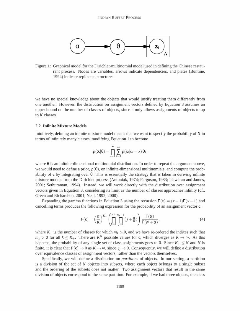
where Discrete(θ) is the multiple-outcome analogue of a Bernoulli event, where the probabilitiesof the outcomes are specified byθ (i.e., P(ci = k|θ) = θk). The dependencies among variables inthis model are shown in Figure 1. Having defined a prior onθ, we can simplify this model byintegrating over all values ofθ rather than representing them explicitly. The marginal probability ofan assignment vectorc, integrating over all values ofθ, is
P(c) =∫
∆K
n
∏i=1
P(ci |θ) p(θ)dθ
=∫
∆K
∏Kk=1 θmk+α/K−1
k
D( αK ,
αK , . . . ,
αK )
dθ
=D(m1+
αK ,m2+
αK , . . . ,mk+
αK )
D( αK ,
αK , . . . ,
αK )
=∏K
k=1 Γ(mk+αK )
Γ( αK )
K
Γ(α)Γ(N+α)
, (3)
wheremk = ∑Ni=1 δ(ci = k) is the number of objects assigned to classk. The tractability of this
integral is a result of the fact that the Dirichlet is conjugate to the multinomial.Equation 3 defines a joint probability distribution for all class assignmentsc in which individual
class assignments are not independent. Rather, they areexchangeable(Bernardo and Smith, 1994),with the probability of an assignment vector remaining the same when the indices of the objects arepermuted. Exchangeability is a desirable property in a distribution over classassignments, because
1188
INDIAN BUFFET PROCESS
θ ziαN
Figure 1: Graphical model for the Dirichlet-multinomial model used in defining the Chinese restau-rant process. Nodes are variables, arrows indicate dependencies,and plates (Buntine,1994) indicate replicated structures.
we have no special knowledge about the objects that would justify treating them differently fromone another. However, the distribution on assignment vectors defined byEquation 3 assumes anupper bound on the number of classes of objects, since it only allows assignments of objects to upto K classes.
2.2 Infinite Mixture Models
Intuitively, defining an infinite mixture model means that we want to specify the probability ofX interms of infinitely many classes, modifying Equation 1 to become
p(X|θ) =N
∏i=1
∞
∑k=1
p(xi |ci = k)θk,
whereθ is an infinite-dimensional multinomial distribution. In order to repeat the argument above,we would need to define a prior,p(θ), on infinite-dimensional multinomials, and compute the prob-ability of c by integrating overθ. This is essentially the strategy that is taken in deriving infinitemixture models from the Dirichlet process (Antoniak, 1974; Ferguson, 1983; Ishwaran and James,2001; Sethuraman, 1994). Instead, we will work directly with the distributionover assignmentvectors given in Equation 3, considering its limit as the number of classes approaches infinity (cf.,Green and Richardson, 2001; Neal, 1992, 2000).
Expanding the gamma functions in Equation 3 using the recursionΓ(x) = (x−1)Γ(x−1) andcancelling terms produces the following expression for the probability of anassignment vectorc:
P(c) =(α
K
)K+
(
K+
∏k=1
mk−1
∏j=1
( j + αK )
)
Γ(α)Γ(N+α)
, (4)
whereK+ is the number of classes for whichmk > 0, and we have re-ordered the indices such thatmk > 0 for all k ≤ K+. There areKN possible values forc, which diverges asK → ∞. As thishappens, the probability of any single set of class assignments goes to 0. SinceK+ ≤ N andN isfinite, it is clear thatP(c)→ 0 asK → ∞, since 1
K → 0. Consequently, we will define a distributionover equivalence classes of assignment vectors, rather than the vectors themselves.
Specifically, we will define a distribution onpartitions of objects. In our setting, a partitionis a division of the set ofN objects into subsets, where each object belongs to a single subsetand the ordering of the subsets does not matter. Two assignment vectors that result in the samedivision of objects correspond to the same partition. For example, if we had three objects, the class
1189
GRIFFITHS AND GHAHRAMANI
assignments{c1,c2,c3}= {1,1,2} would correspond to the same partition as{2,2,1}, since all thatdiffers between these two cases is the labels of the classes. A partition thus defines an equivalenceclass of assignment vectors, which we denote[c], with two assignment vectors belonging to the sameequivalence class if they correspond to the same partition. A distribution over partitions is sufficientto allow us to define an infinite mixture model, provided the prior distribution on the parameters isthe same for all classes. In this case, these equivalence classes of class assignments are the same asthose induced by identifiability:p(X|c) is the same for all assignment vectorsc that correspond tothe same partition, so we can apply statistical inference at the level of partitions rather than the levelof assignment vectors.
Assume we have a partition ofN objects intoK+ subsets, and we haveK = K0 +K+ classlabels that can be applied to those subsets. Then there areK!
K0! assignment vectorsc that belong tothe equivalence class defined by that partition,[c]. We can define a probability distribution overpartitions by summing over all class assignments that belong to the equivalenceclass defined byeach partition. The probability of each of those class assignments is equal under the distributionspecified by Equation 4, so we obtain
P([c]) = ∑c∈[c]
P(c)
=K!K0!
(αK
)K+
(
K+
∏k=1
mk−1
∏j=1
( j + αK )
)
Γ(α)Γ(N+α)
.
Rearranging the first two terms, we can compute the limit of the probability of a partition asK → ∞,which is
limK→∞
αK+ ·K!
K0! KK+·
(
K+
∏k=1
mk−1
∏j=1
( j + αK )
)
·Γ(α)
Γ(N+α)
= αK+ · 1 ·
(
K+
∏k=1
(mk−1)!
)
·Γ(α)
Γ(N+α). (5)
The details of the steps taken in computing this limit are given in Appendix A. These limitingprobabilities define a valid distribution over partitions, and thus over equivalence classes of classassignments, providing a prior over class assignments for an infinite mixture model. Objects areexchangeable under this distribution, just as in the finite case: the probabilityof a partition is notaffected by the ordering of the objects, since it depends only on the counts mk.
As noted above, the distribution over partitions specified by Equation 5 can be derived in a vari-ety of ways—by taking limits (Green and Richardson, 2001; Neal, 1992, 2000), from the Dirichletprocess (Blackwell and MacQueen, 1973), or from other equivalent stochastic processes (Ishwaranand James, 2001; Sethuraman, 1994). We will briefly discuss a simple process that produces thesame distribution over partitions: the Chinese restaurant process.
2.3 The Chinese Restaurant Process
The Chinese restaurant process (CRP) was named by Jim Pitman and Lester Dubins, based upona metaphor in which the objects are customers in a restaurant, and the classesare the tables atwhich they sit (the process first appears in Aldous 1985, where it is attributed to Pitman, although
1190
INDIAN BUFFET PROCESS
...
2
10
6 7
93
1 4
8 5
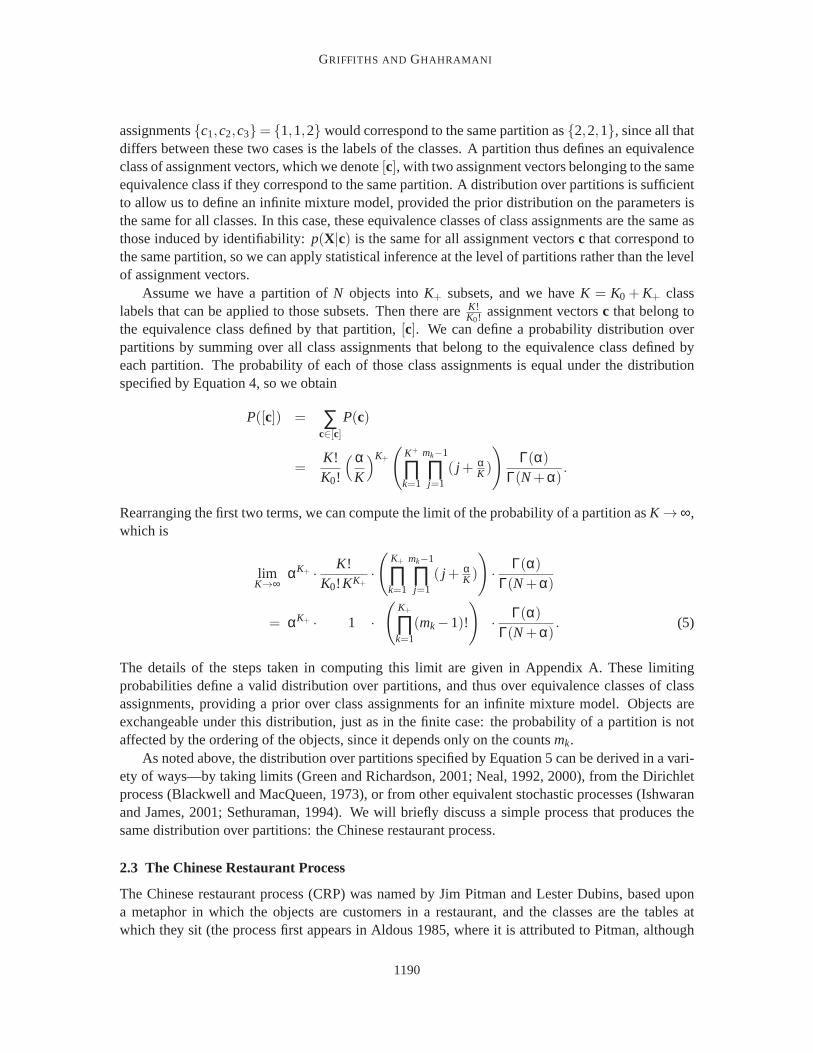
Figure 2: A partition induced by the Chinese restaurant process. Numbers indicate customers (ob-jects), circles indicate tables (classes).
it is identical to the extended Polya urn scheme introduced by Blackwell and MacQueen 1973).Imagine a restaurant with an infinite number of tables, each with an infinite number of seats.2 Thecustomers enter the restaurant one after another, and each choose a table at random. In the CRPwith parameterα, each customer chooses an occupied table with probability proportional to thenumber of occupants, and chooses the next vacant table with probability proportional toα. Forexample, Figure 2 shows the state of a restaurant after 10 customers havechosen tables using thisprocedure. The first customer chooses the first table with probabilityα
α = 1. The second customerchooses the first table with probability11+α , and the second table with probabilityα1+α . After thesecond customer chooses the second table, the third customer chooses thefirst table with probability
12+α , the second table with probability1
2+α , and the third table with probabilityα2+α . This process
continues until all customers have seats, defining a distribution over allocations of people to tables,and, more generally, objects to classes. Extensions of the CRP and connections to other stochasticprocesses are pursued in depth by Pitman (2002).
The distribution over partitions induced by the CRP is the same as that given in Equation 5. Ifwe assume an ordering on ourN objects, then we can assign them to classes sequentially using themethod specified by the CRP, letting objects play the role of customers and classes play the role oftables. Theith object would be assigned to thekth class with probability
P(ci = k|c1,c2, . . . ,ci−1) =
{ mki−1+α k≤ K+
αi−1+α k= K+1
wheremk is the number of objects currently assigned to classk, andK+ is the number of classes forwhich mk > 0. If all N objects are assigned to classes via this process, the probability of a partitionof objectsc is that given in Equation 5. The CRP thus provides an intuitive means of specifying aprior for infinite mixture models, as well as revealing that there is a simple sequential process bywhich exchangeable class assignments can be generated.
2.4 Inference by Gibbs Sampling
Inference in an infinite mixture model is only slightly more complicated than inference in a mixturemodel with a finite, fixed number of classes. The standard algorithm used for inference in infinitemixture models is Gibbs sampling (Bush and MacEachern, 1996; Neal, 2000). Gibbs sampling
2. Pitman and Dubins, both statisticians at the University of California, Berkeley, were inspired by the apparently infinitecapacity of Chinese restaurants in San Francisco when they named the process.
1191

GRIFFITHS AND GHAHRAMANI
is a Markov chain Monte Carlo (MCMC) method, in which variables are successively sampledfrom their distributions when conditioned on the current values of all othervariables (Geman andGeman, 1984). This process defines a Markov chain, which ultimately converges to the distributionof interest (see Gilks et al., 1996). Recent work has also explored variational inference algorithmsfor these models (Blei and Jordan, 2006), a topic we will return to later in thepaper.
Implementing a Gibbs sampler requires deriving the full conditional distributionfor all variablesto be sampled. In a mixture model, these variables are the class assignmentsc. The relevant fullconditional distribution isP(ci |c−i ,X), the probability distribution overci conditioned on the classassignments of all other objects,c−i , and the data,X. By applying Bayes’ rule, this distribution canbe expressed as
P(ci = k|c−i ,X) ∝ p(X|c)P(ci = k|c−i),
where only the second term on the right hand side depends upon the distribution over class assign-ments,P(c). Here we assume that the parameters associated with each class can be integrated out,so we that the probability of the data depends only on the class assignment. This is possible when aconjugate prior is used on these parameters. For details, and alternative algorithms that can be usedwhen this assumption is violated, see Neal (2000).
In a finite mixture model withP(c) defined as in Equation 3, we can computeP(ci = k|c−i) byintegrating overθ, obtaining
P(ci = k|c−i) =∫
P(ci = k|θ)p(θ|c−i)dθ
=m−i,k+
αK
N−1+α, (6)
wherem−i,k is the number of objects assigned to classk, not including objecti. This is the posteriorpredictive distribution for a multinomial distribution with a Dirichlet prior.
In an infinite mixture model with a distribution over class assignments defined as inEquation 5,we can use exchangeability to find the full conditional distribution. Since it is exchangeable,P([c])is unaffected by the ordering of objects. Thus, we can choose an ordering in which theith objectis the last to be assigned to a class. It follows directly from the definition of theChinese restaurantprocess that
P(ci = k|c−i) =
m−i,k
N−1+α m−i,k > 0α
N−1+α k= K−i,++10 otherwise
(7)
whereK−i,+ is the number of classes for whichm−i,k > 0. The same result can be found by takingthe limit of the full conditional distribution in the finite model, given by Equation 6 (Neal, 2000).
When combined with some choice ofp(X|c), Equations 6 and 7 are sufficient to define Gibbssamplers for finite and infinite mixture models respectively. Demonstrations of Gibbs samplingin infinite mixture models are provided by Neal (2000) and Rasmussen (2000). Similar MCMCalgorithms are presented in Bush and MacEachern (1996), West et al. (1994), Escobar and West(1995) and Ishwaran and James (2001). Algorithms that go beyond the local changes in classassignments allowed by a Gibbs sampler are given by Jain and Neal (2004)and Dahl (2003).
2.5 Summary
Our review of infinite mixture models serves three purposes: it shows that infinite statistical modelscan be defined by specifying priors over infinite combinatorial objects; it illustrates how these priors
1192
INDIAN BUFFET PROCESS
can be derived by taking the limit of priors for finite models; and it demonstrates that inference inthese models can remain possible, despite the large hypothesis spaces they imply. However, infinitemixture models are still fundamentally limited in their representation of objects, assuming that eachobject can only belong to a single class. In the next two sections, we use theinsights underlyinginfinite mixture models to derive methods for representing objects in terms of infinitely many latentfeatures, leading us to derive a distribution on infinite binary matrices.
3. Latent Feature Models
In a latent feature model, each object is represented by a vector of latentfeature valuesf i , and thepropertiesxi are generated from a distribution determined by those latent feature values. Latent fea-ture values can be continuous, as in factor analysis (Roweis and Ghahramani, 1999) and probabilis-tic principal component analysis (PCA; Tipping and Bishop, 1999), or discrete, as in cooperativevector quantization (CVQ; Zemel and Hinton, 1994; Ghahramani, 1995). In the remainder of thissection, we will assume that feature values are continuous. Using the matrixF =
[
fT1 fT
2 · · · fTN
]Tto
indicate the latent feature values for allN objects, the model is specified by a prior over features,p(F), and a distribution over observed property matrices conditioned on those features,p(X|F). Aswith latent class models, these distributions can be dealt with separately:p(F) specifies the numberof features, their probability, and the distribution over values associated with each feature, whilep(X|F) determines how these features relate to the properties of objects. Our focus will be onp(F),showing how such a prior can be defined without placing an upper boundon the number of features.
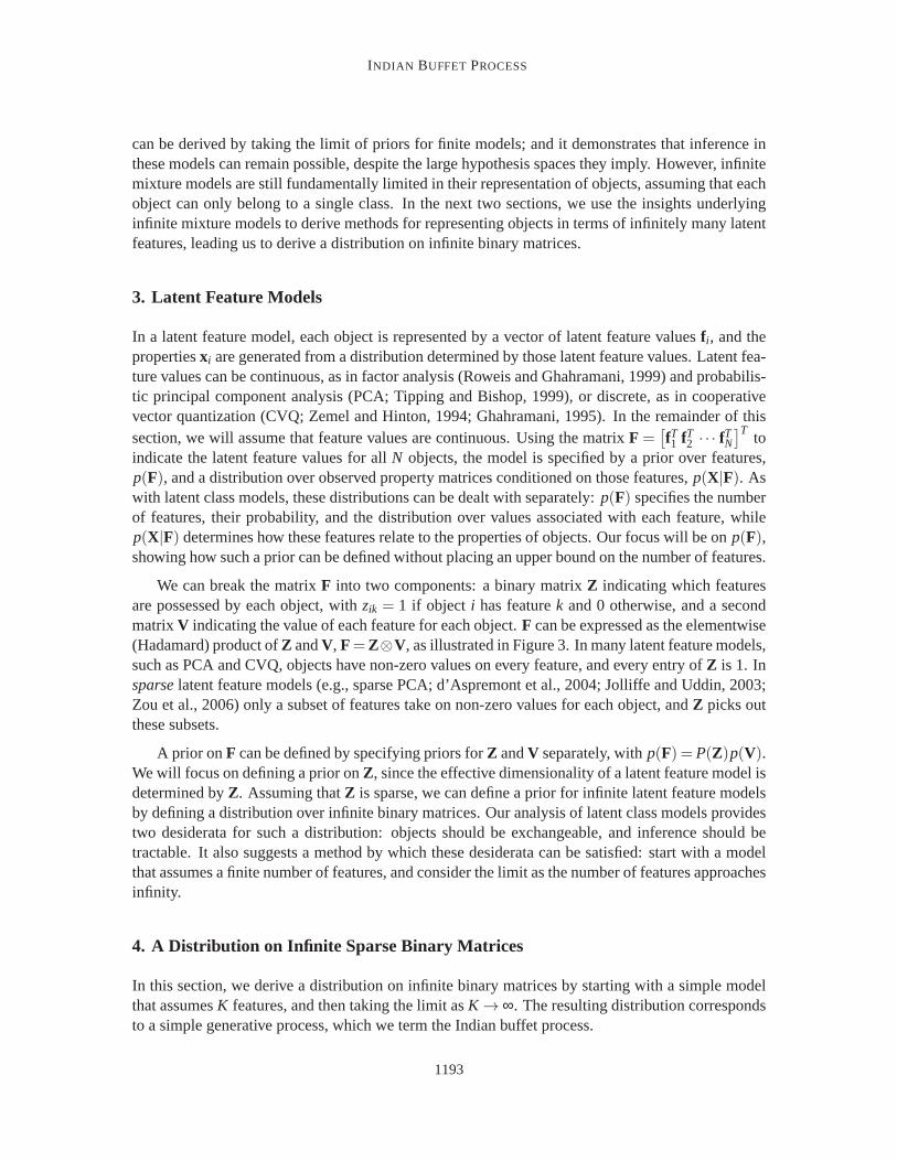
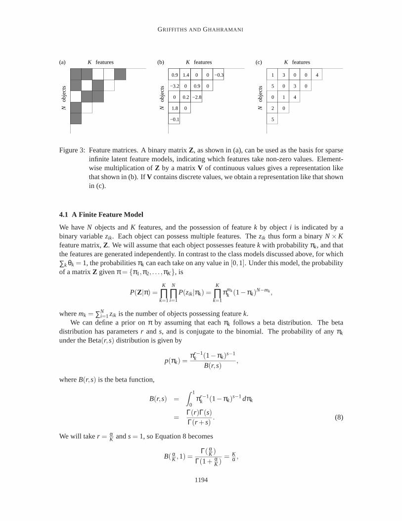
We can break the matrixF into two components: a binary matrixZ indicating which featuresare possessed by each object, withzik = 1 if object i has featurek and 0 otherwise, and a secondmatrixV indicating the value of each feature for each object.F can be expressed as the elementwise(Hadamard) product ofZ andV, F=Z⊗V, as illustrated in Figure 3. In many latent feature models,such as PCA and CVQ, objects have non-zero values on every feature, and every entry ofZ is 1. Insparselatent feature models (e.g., sparse PCA; d’Aspremont et al., 2004; Jolliffe and Uddin, 2003;Zou et al., 2006) only a subset of features take on non-zero values for each object, andZ picks outthese subsets.
A prior onF can be defined by specifying priors forZ andV separately, withp(F) =P(Z)p(V).We will focus on defining a prior onZ, since the effective dimensionality of a latent feature model isdetermined byZ. Assuming thatZ is sparse, we can define a prior for infinite latent feature modelsby defining a distribution over infinite binary matrices. Our analysis of latent class models providestwo desiderata for such a distribution: objects should be exchangeable, and inference should betractable. It also suggests a method by which these desiderata can be satisfied: start with a modelthat assumes a finite number of features, and consider the limit as the number of features approachesinfinity.
4. A Distribution on Infinite Sparse Binary Matrices
In this section, we derive a distribution on infinite binary matrices by starting witha simple modelthat assumesK features, and then taking the limit asK → ∞. The resulting distribution correspondsto a simple generative process, which we term the Indian buffet process.
1193
GRIFFITHS AND GHAHRAMANI
(c)ob
ject
sN
K features
obje
cts
N
K features
0
0
0
0 0
0
−0.1
1.8
−3.2
0.9
0.9
−0.3
0.2 −2.8
1.4
obje
cts
N
K features
5
0
0
0
0 0
0
2
5
1
1
4
4
3
3
(a) (b)
Figure 3: Feature matrices. A binary matrixZ, as shown in (a), can be used as the basis for sparseinfinite latent feature models, indicating which features take non-zero values. Element-wise multiplication ofZ by a matrixV of continuous values gives a representation likethat shown in (b). IfV contains discrete values, we obtain a representation like that shownin (c).
4.1 A Finite Feature Model
We haveN objects andK features, and the possession of featurek by object i is indicated by abinary variablezik. Each object can possess multiple features. Thezik thus form a binaryN×Kfeature matrix,Z. We will assume that each object possesses featurek with probabilityπk, and thatthe features are generated independently. In contrast to the class modelsdiscussed above, for which∑k θk = 1, the probabilitiesπk can each take on any value in[0,1]. Under this model, the probabilityof a matrixZ givenπ = {π1,π2, . . . ,πK}, is
P(Z|π) =K
∏k=1
N
∏i=1
P(zik|πk) =K
∏k=1
πmkk (1−πk)
N−mk,
wheremk = ∑Ni=1zik is the number of objects possessing featurek.
We can define a prior onπ by assuming that eachπk follows a beta distribution. The betadistribution has parametersr ands, and is conjugate to the binomial. The probability of anyπk
under the Beta(r,s) distribution is given by
p(πk) =πr−1
k (1−πk)s−1
B(r,s),
whereB(r,s) is the beta function,
B(r,s) =∫ 1
0πr−1
k (1−πk)s−1dπk
=Γ(r)Γ(s)Γ(r +s)
. (8)
We will taker = αK ands= 1, so Equation 8 becomes
B( αK ,1) =
Γ( αK )
Γ(1+ αK )
= Kα ,
1194
INDIAN BUFFET PROCESS
zikπkαN
K
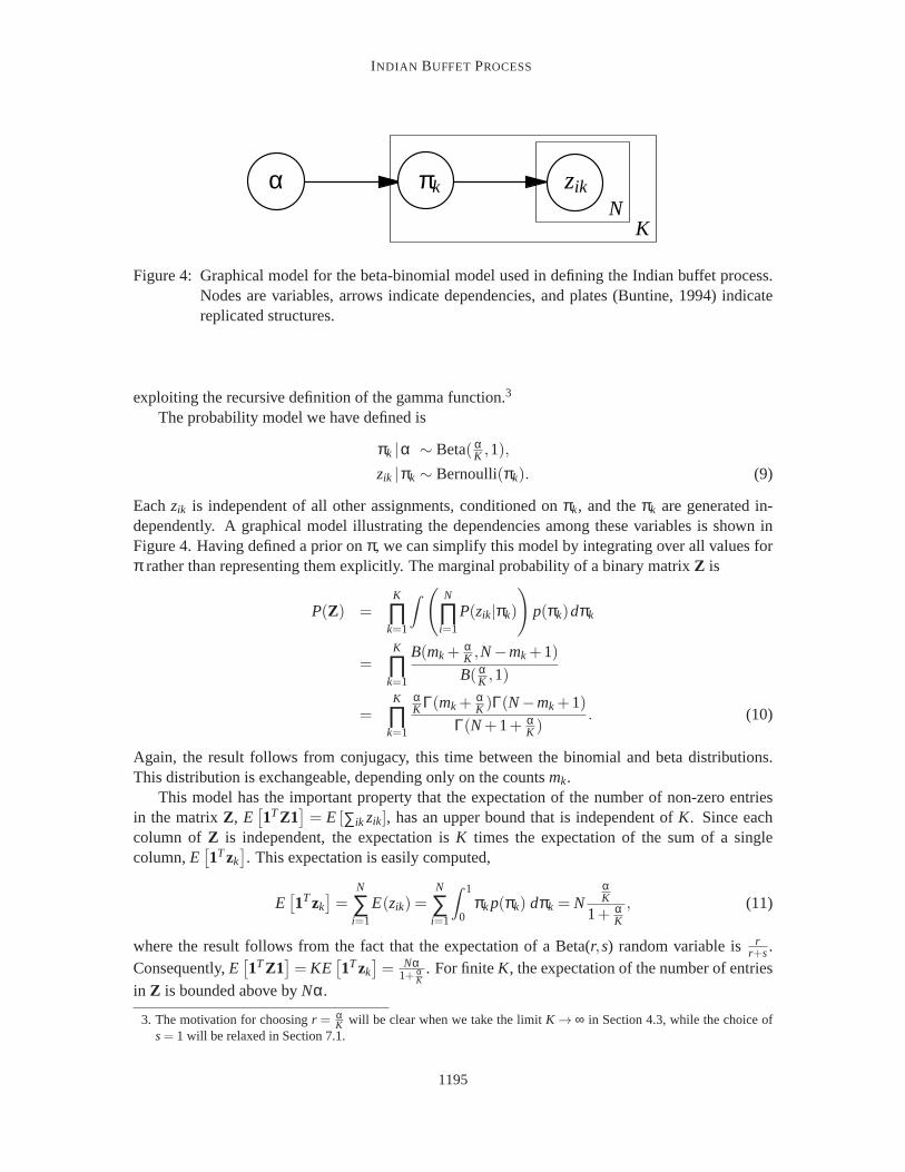
Figure 4: Graphical model for the beta-binomial model used in defining the Indian buffet process.Nodes are variables, arrows indicate dependencies, and plates (Buntine, 1994) indicatereplicated structures.
exploiting the recursive definition of the gamma function.3
The probability model we have defined is
πk |α ∼ Beta( αK ,1),
zik |πk ∼ Bernoulli(πk). (9)
Eachzik is independent of all other assignments, conditioned onπk, and theπk are generated in-dependently. A graphical model illustrating the dependencies among these variables is shown inFigure 4. Having defined a prior onπ, we can simplify this model by integrating over all values forπ rather than representing them explicitly. The marginal probability of a binarymatrixZ is
P(Z) =K
∏k=1
∫ ( N
∏i=1
P(zik|πk)
)
p(πk)dπk
=K
∏k=1
B(mk+αK ,N−mk+1)
B( αK ,1)
=K
∏k=1
αK Γ(mk+
αK )Γ(N−mk+1)
Γ(N+1+ αK )
. (10)
Again, the result follows from conjugacy, this time between the binomial and beta distributions.This distribution is exchangeable, depending only on the countsmk.
This model has the important property that the expectation of the number of non-zero entriesin the matrixZ, E
[
1TZ1]
= E [∑ik zik], has an upper bound that is independent ofK. Since eachcolumn of Z is independent, the expectation isK times the expectation of the sum of a singlecolumn,E
[
1Tzk]
. This expectation is easily computed,
E[
1Tzk]
=N
∑i=1
E(zik) =N
∑i=1
∫ 1
0πkp(πk) dπk = N
αK
1+ αK
, (11)
where the result follows from the fact that the expectation of a Beta(r,s) random variable is rr+s.
Consequently,E[
1TZ1]
= KE[
1Tzk]
= Nα1+ α
K. For finiteK, the expectation of the number of entries
in Z is bounded above byNα.
3. The motivation for choosingr = αK will be clear when we take the limitK → ∞ in Section 4.3, while the choice of
s= 1 will be relaxed in Section 7.1.
1195
GRIFFITHS AND GHAHRAMANI
lof
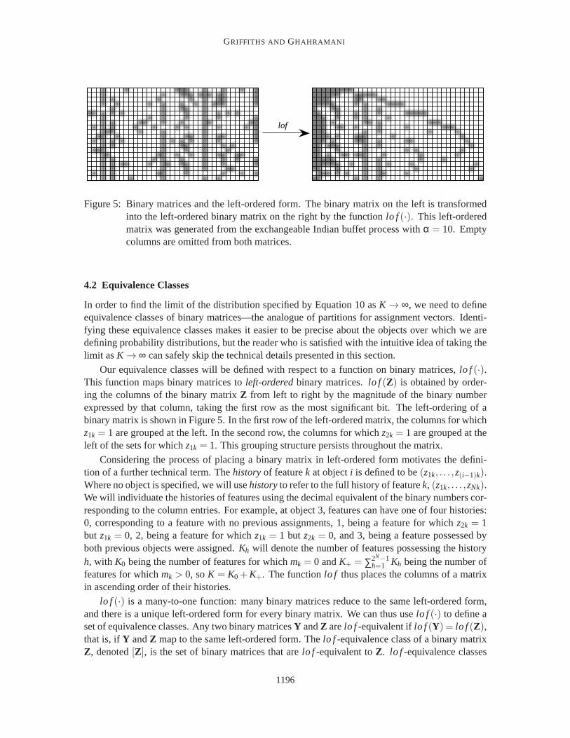
Figure 5: Binary matrices and the left-ordered form. The binary matrix on theleft is transformedinto the left-ordered binary matrix on the right by the functionlo f (·). This left-orderedmatrix was generated from the exchangeable Indian buffet process withα = 10. Emptycolumns are omitted from both matrices.
4.2 Equivalence Classes
In order to find the limit of the distribution specified by Equation 10 asK → ∞, we need to defineequivalence classes of binary matrices—the analogue of partitions for assignment vectors. Identi-fying these equivalence classes makes it easier to be precise about the objects over which we aredefining probability distributions, but the reader who is satisfied with the intuitive idea of taking thelimit as K → ∞ can safely skip the technical details presented in this section.
Our equivalence classes will be defined with respect to a function on binary matrices,lo f (·).This function maps binary matrices toleft-orderedbinary matrices.lo f (Z) is obtained by order-ing the columns of the binary matrixZ from left to right by the magnitude of the binary numberexpressed by that column, taking the first row as the most significant bit. The left-ordering of abinary matrix is shown in Figure 5. In the first row of the left-ordered matrix,the columns for whichz1k = 1 are grouped at the left. In the second row, the columns for whichz2k = 1 are grouped at theleft of the sets for whichz1k = 1. This grouping structure persists throughout the matrix.
Considering the process of placing a binary matrix in left-ordered form motivates the defini-tion of a further technical term. Thehistoryof featurek at objecti is defined to be(z1k, . . . ,z(i−1)k).Where no object is specified, we will usehistoryto refer to the full history of featurek, (z1k, . . . ,zNk).We will individuate the histories of features using the decimal equivalent ofthe binary numbers cor-responding to the column entries. For example, at object 3, features can have one of four histories:0, corresponding to a feature with no previous assignments, 1, being a feature for whichz2k = 1but z1k = 0, 2, being a feature for whichz1k = 1 but z2k = 0, and 3, being a feature possessed byboth previous objects were assigned.Kh will denote the number of features possessing the historyh, with K0 being the number of features for whichmk = 0 andK+ = ∑2N−1
h=1 Kh being the number offeatures for whichmk > 0, soK = K0+K+. The functionlo f thus places the columns of a matrixin ascending order of their histories.
lo f (·) is a many-to-one function: many binary matrices reduce to the same left-ordered form,and there is a unique left-ordered form for every binary matrix. We can thus uselo f (·) to define aset of equivalence classes. Any two binary matricesY andZ arelo f -equivalent iflo f (Y) = lo f (Z),that is, ifY andZ map to the same left-ordered form. Thelo f -equivalence class of a binary matrixZ, denoted[Z], is the set of binary matrices that arelo f -equivalent toZ. lo f -equivalence classes
1196
INDIAN BUFFET PROCESS
are preserved through permutation of either the rows or the columns of a matrix, provided the samepermutations are applied to the other members of the equivalence class. Performing inference atthe level oflo f -equivalence classes is appropriate in models where feature order is not identifiable,with p(X|F) being unaffected by the order of the columns ofF. Any model in which the probabilityof X is specified in terms of a linear function ofF, such as PCA or CVQ, has this property.
We need to evaluate the cardinality of[Z], being the number of matrices that map to the sameleft-ordered form. The columns of a binary matrix are not guaranteed to beunique: since an objectcan possess multiple features, it is possible for two features to be possessed by exactly the same setof objects. The number of matrices in[Z] is reduced ifZ contains identical columns, since somere-orderings of the columns ofZ result in exactly the same matrix. Taking this into account, the
cardinality of[Z] is(
KK0...K2N−1
)
= K!
∏2N−1h=0 Kh!
, whereKh is the count of the number of columns with
full history h.lo f -equivalence classes play the same role for binary matrices as partitions dofor assignment
vectors: they collapse together all binary matrices (assignment vectors) that differ only in columnordering (class labels). This relationship can be made precise by examiningthe lo f -equivalenceclasses of binary matrices constructed from assignment vectors. Definetheclass matrixgeneratedby an assignment vectorc to be a binary matrixZ wherezik = 1 if and only if ci = k. It is straight-forward to show that the class matrices generated by two assignment vectors that correspond to thesame partition belong to the samelo f -equivalence class, and vice versa.
4.3 Taking the Infinite Limit
Under the distribution defined by Equation 10, the probability of a particularlo f -equivalence classof binary matrices,[Z], is
P([Z]) = ∑Z∈[Z]
P(Z)
=K!
∏2N−1h=0 Kh!
K
∏k=1
αK Γ(mk+
αK )Γ(N−mk+1)
Γ(N+1+ αK )
. (12)
In order to take the limit of this expression asK → ∞, we will divide the columns ofZ into twosubsets, corresponding to the features for whichmk = 0 and the features for whichmk > 0. Re-ordering the columns such thatmk > 0 if k ≤ K+, andmk = 0 otherwise, we can break the productin Equation 12 into two parts, corresponding to these two subsets. The product thus becomes
K
∏k=1
αK Γ(mk+
αK )Γ(N−mk+1)
Γ(N+1+ αK )
=
( αK Γ( α
K )Γ(N+1)
Γ(N+1+ αK )
)K−K+ K+
∏k=1
αK Γ(mk+
αK )Γ(N−mk+1)
Γ(N+1+ αK )
=
( αK Γ( α
K )Γ(N+1)
Γ(N+1+ αK )
)K K+
∏k=1
Γ(mk+αK )Γ(N−mk+1)
Γ( αK )Γ(N+1)
=
(
N!
∏Nj=1( j + α
K )
)K(α
K
)K+K+
∏k=1
(N−mk)! ∏mk−1j=1 ( j + α
K )
N!, (13)
1197
GRIFFITHS AND GHAHRAMANI
where we have used the fact thatΓ(x) = (x−1)Γ(x−1) for x > 1. Substituting Equation 13 intoEquation 12 and rearranging terms, we can compute our limit
limK→∞
αK+
∏2N−1h=1 Kh!
·K!
K0! KK+·
(
N!
∏Nj=1( j + α
K )
)K
·K+
∏k=1
(N−mk)! ∏mk−1j=1 ( j + α
K )
N!
=αK+
∏2N−1h=1 Kh!
· 1 · exp{−αHN} ·K+
∏k=1
(N−mk)!(mk−1)!N!
, (14)
whereHN is theNth harmonic number,HN = ∑Nj=1
1j . The details of the steps taken in computing
this limit are given in Appendix A. Again, this distribution is exchangeable: neither the number ofidentical columns nor the column sums are affected by the ordering on objects.
4.4 The Indian Buffet Process
The probability distribution defined in Equation 14 can be derived from a simple stochastic process.As with the CRP, this process assumes an ordering on the objects, generating the matrix sequen-tially using this ordering. We will also use a culinary metaphor in defining our stochastic process,appropriately adjusted for geography.4 Many Indian restaurants offer lunchtime buffets with anapparently infinite number of dishes. We can define a distribution over infinitebinary matrices byspecifying a procedure by which customers (objects) choose dishes (features).
In our Indian buffet process (IBP),N customers enter a restaurant one after another. Each cus-tomer encounters a buffet consisting of infinitely many dishes arranged in aline. The first customerstarts at the left of the buffet and takes a serving from each dish, stopping after a Poisson(α) numberof dishes as his plate becomes overburdened. Theith customer moves along the buffet, samplingdishes in proportion to their popularity, serving himself with probabilitymk
i , wheremk is the numberof previous customers who have sampled a dish. Having reached the end of all previous sampleddishes, theith customer then tries a Poisson(α
i ) number of new dishes.We can indicate which customers chose which dishes using a binary matrixZ with N rows and
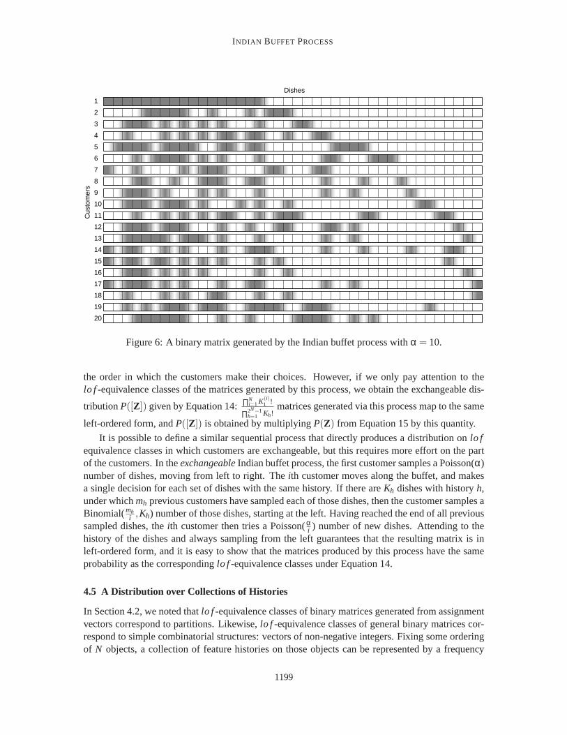
infinitely many columns, wherezik = 1 if the ith customer sampled thekth dish. Figure 6 showsa matrix generated using the IBP withα = 10. The first customer tried 17 dishes. The secondcustomer tried 7 of those dishes, and then tried 3 new dishes. The third customer tried 3 dishes triedby both previous customers, 5 dishes tried by only the first customer, and 2new dishes. Verticallyconcatenating the choices of the customers produces the binary matrix shown in the figure.
UsingK(i)1 to indicate the number of new dishes sampled by theith customer, the probability of
any particular matrix being produced by this process is
P(Z) =αK+
∏Ni=1K(i)
1 !exp{−αHN}
K+
∏k=1
(N−mk)!(mk−1)!N!
. (15)
As can be seen from Figure 6, the matrices produced by this process aregenerally not in left-orderedform. However, these matrices are also not ordered arbitrarily becausethe Poisson draws alwaysresult in choices of new dishes that are to the right of the previously sampled dishes. Customersare not exchangeable under this distribution, as the number of dishes counted asK(i)
1 depends upon
4. This work was started when both authors were at the Gatsby Computational Neuroscience Unit in London, where theIndian buffet is the dominant culinary metaphor.
1198
INDIAN BUFFET PROCESS
Dishes
1
2
3
4
5
6
7
8
9
10
11
12
Cus
tom
ers
13
14
15
16
17
18
19
20
Figure 6: A binary matrix generated by the Indian buffet process withα = 10.
the order in which the customers make their choices. However, if we only payattention to thelo f -equivalence classes of the matrices generated by this process, we obtain the exchangeable dis-
tributionP([Z]) given by Equation 14:∏Ni=1 K(i)
1 !
∏2N−1h=1 Kh!
matrices generated via this process map to the same
left-ordered form, andP([Z]) is obtained by multiplyingP(Z) from Equation 15 by this quantity.
It is possible to define a similar sequential process that directly produces adistribution onlo fequivalence classes in which customers are exchangeable, but this requires more effort on the partof the customers. In theexchangeableIndian buffet process, the first customer samples a Poisson(α)number of dishes, moving from left to right. Theith customer moves along the buffet, and makesa single decision for each set of dishes with the same history. If there areKh dishes with historyh,under whichmh previous customers have sampled each of those dishes, then the customer samples aBinomial(mh
i ,Kh) number of those dishes, starting at the left. Having reached the end of all previoussampled dishes, theith customer then tries a Poisson(α
i ) number of new dishes. Attending to thehistory of the dishes and always sampling from the left guarantees that theresulting matrix is inleft-ordered form, and it is easy to show that the matrices produced by this process have the sameprobability as the correspondinglo f -equivalence classes under Equation 14.
4.5 A Distribution over Collections of Histories
In Section 4.2, we noted thatlo f -equivalence classes of binary matrices generated from assignmentvectors correspond to partitions. Likewise,lo f -equivalence classes of general binary matrices cor-respond to simple combinatorial structures: vectors of non-negative integers. Fixing some orderingof N objects, a collection of feature histories on those objects can be represented by a frequency
1199
GRIFFITHS AND GHAHRAMANI
vectorK = (K1, . . . ,K2N−1), indicating the number of times each history appears in the collection.A collection of feature histories can be translated into a left-ordered binarymatrix by horizontallyconcatenating an appropriate number of copies of the binary vector representing each history intoa matrix. A left-ordered binary matrix can be translated into a collection of feature histories bycounting the number of times each history appears in that matrix. Since partitionsare a subsetof all collections of histories—namely those collections in which each object appears in only onehistory—this process is strictly more general than the CRP.
This connection betweenlo f -equivalence classes of feature matrices and collections of featurehistories suggests another means of deriving the distribution specified by Equation 14, operatingdirectly on the frequencies of these histories. We can define a distribution on vectors of non-negativeintegersK by assuming that eachKh is generated independently from a Poisson distribution withparameterαB(mh,N−mh+1) = α (mh−1)!(N−mh)!
N! wheremh is the number of non-zero elements inthe historyh. This gives
P(K) =2N−1
∏h=1
(
α (mh−1)!(N−mh)!N!
)Kh
Kh!exp
{
−α(mh−1)!(N−mh)!
N!
}
=α∑2N−1
h=1 Kh
∏2N−1h=1 Kh!
exp{−αHN}2N−1
∏h=1
(
(mh−1)!(N−mh)!N!
)Kh
,
which is easily seen to be the same asP([Z]) in Equation 14. The harmonic number in the expo-
nential term is obtained by summing(mh−1)!(N−m)!N! over all historiesh. There are
(
Nj
)
histories for
whichmh = j, so we have
2N−1
∑h=1
(mh−1)!(N−mh)!N!
=N
∑j=1
(Nj)( j −1)!(N− j)!
N!=
N
∑j=1
1j= HN. (16)
4.6 Properties of this Distribution
These different views of the distribution specified by Equation 14 make it straightforward to derivesome of its properties. First, the effective dimension of the model,K+, follows a Poisson(αHN)distribution. This is easily shown using the generative process describedin Section 4.5:K+ =
∑2N−1h=1 Kh, and under this process is thus the sum of a set of Poisson distributions. The sum of a set
of Poisson distributions is a Poisson distribution with parameter equal to the sumof the parametersof its components. Using Equation 16, this isαHN. Alternatively, we can use the fact that thenumber of new columns generated at theith row is Poisson(α
i ), with the total number of columnsbeing the sum of these quantities.
A second property of this distribution is that the number of features possessed by each objectfollows a Poisson(α) distribution. This follows from the definition of the exchangeable IBP. Thefirst customer chooses a Poisson(α) number of dishes. By exchangeability, all other customers mustalso choose a Poisson(α) number of dishes, since we can always specify an ordering on customerswhich begins with a particular customer.
Finally, it is possible to show thatZ remains sparse asK → ∞. The simplest way to do this is toexploit the previous result: if the number of features possessed by eachobject follows a Poisson(α)distribution, then the expected number of entries inZ is Nα. This is consistent with the quantity
1200
INDIAN BUFFET PROCESS
obtained by taking the limit of this expectation in the finite model, which is given in Equation 11:limK→∞ E
[
1TZ1]
= limK→∞Nα
1+ αK= Nα.
4.7 Inference by Gibbs Sampling
We have defined a distribution over infinite binary matrices that satisfies one of our desiderata—objects (the rows of the matrix) are exchangeable under this distribution. Itremains to be shownthat inference in infinite latent feature models is tractable, as was the case for infinite mixture mod-els. We will derive a Gibbs sampler for sampling from the distribution defined by the IBP, whichsuggests a strategy for inference in latent feature models in which the exchangeable IBP is used asa prior. We will consider alternative inference algorithms later in the paper.
To sample from the distribution defined by the IBP, we need to compute the conditional distri-bution P(zik = 1|Z−(ik)), whereZ−(ik) denotes the entries ofZ other thanzik. In the finite model,whereP(Z) is given by Equation 10, it is straightforward to compute the conditional distributionfor anyzik. Integrating overπk gives
P(zik = 1|z−i,k) =∫ 1
0P(zik|πk)p(πk|z−i,k)dπk
=m−i,k+
αK
N+ αK
, (17)
wherez−i,k is the set of assignments of other objects, not includingi, for featurek, andm−i,k is thenumber of objects possessing featurek, not includingi. We need only condition onz−i,k rather thanZ−(ik) because the columns of the matrix are generated independently under this prior.
In the infinite case, we can derive the conditional distribution from the exchangeable IBP. Choos-ing an ordering on objects such that theith object corresponds to the last customer to visit the buffet,we obtain
P(zik = 1|z−i,k) =m−i,k
N, (18)
for anyk such thatm−i,k > 0. The same result can be obtained by taking the limit of Equation 17asK → ∞. Similarly the number of new features associated with objecti should be drawn from aPoisson(αN ) distribution. This can also be derived from Equation 17, using the same kind of limitingargument as that presented above to obtain the terms of the Poisson.
This analysis results in a simple Gibbs sampling algorithm for generating samples from thedistribution defined by the IBP. We start with an arbitrary binary matrix. We then iterate through therows of the matrix,i. For each columnk, if m−i,k is greater than 0 we setzik = 1 with probabilitygiven by Equation 18. Otherwise, we delete that column. At the end of the row, we add Poisson(α
N )new columns that have ones in that row. After sufficiently many passes through the rows, theresulting matrix will be a draw from the distributionP(Z) given by Equation 15.
This algorithm suggests a heuristic strategy for sampling from the posterior distributionP(Z|X)in a model that uses the IBP to define a prior onZ. In this case, we need to sample from the fullconditional distribution
P(zik = 1|Z−(ik),X) ∝ p(X|Z)P(zik = 1|Z−(ik))
wherep(X|Z) is the likelihood function for the model, and we assume that parameters of the like-lihood have been integrated out. We can proceed as in the Gibbs sampler given above, simply
1201
GRIFFITHS AND GHAHRAMANI
incorporating the likelihood term when samplingzik for columns for whichm−i,k is greater than 0and drawing the new columns from a distribution where the prior is Poisson(α
N ) and the likelihoodis given byP(X|Z).5
5. An Example: A Linear-Gaussian Latent Feature Model with Binary Features
We have derived a prior for infinite sparse binary matrices, and indicatedhow statistical inferencecan be done in models defined using this prior. In this section, we will show how this prior can beput to use in models for unsupervised learning, illustrating some of the issuesthat can arise in thisprocess. We will describe a simple linear-Gaussian latent feature model, in which the features arebinary. As above, we will start with a finite model and then consider the infinitelimit.
5.1 A Finite Linear-Gaussian Model
In our finite model, theD-dimensional vector of properties of an objecti, xi is generated from aGaussian distribution with meanziA and covariance matrixΣX = σ2
XI , wherezi is aK-dimensionalbinary vector, andA is aK×D matrix of weights. In matrix notation,E [X] = ZA . If Z is a featurematrix, this is a form of binary factor analysis. The distribution ofX givenZ, A, andσX is matrixGaussian:
p(X|Z,A,σX) =1
(2πσ2X)
ND/2exp{−
1
2σ2X
tr((X−ZA)T(X−ZA))} (19)
where tr(·) is the trace of a matrix. This makes it easy to integrate out the model parametersA. Todo so, we need to define a prior onA, which we also take to be matrix Gaussian:
p(A|σA) =1
(2πσ2A)
KD/2exp{−
1
2σ2A
tr(ATA)}, (20)
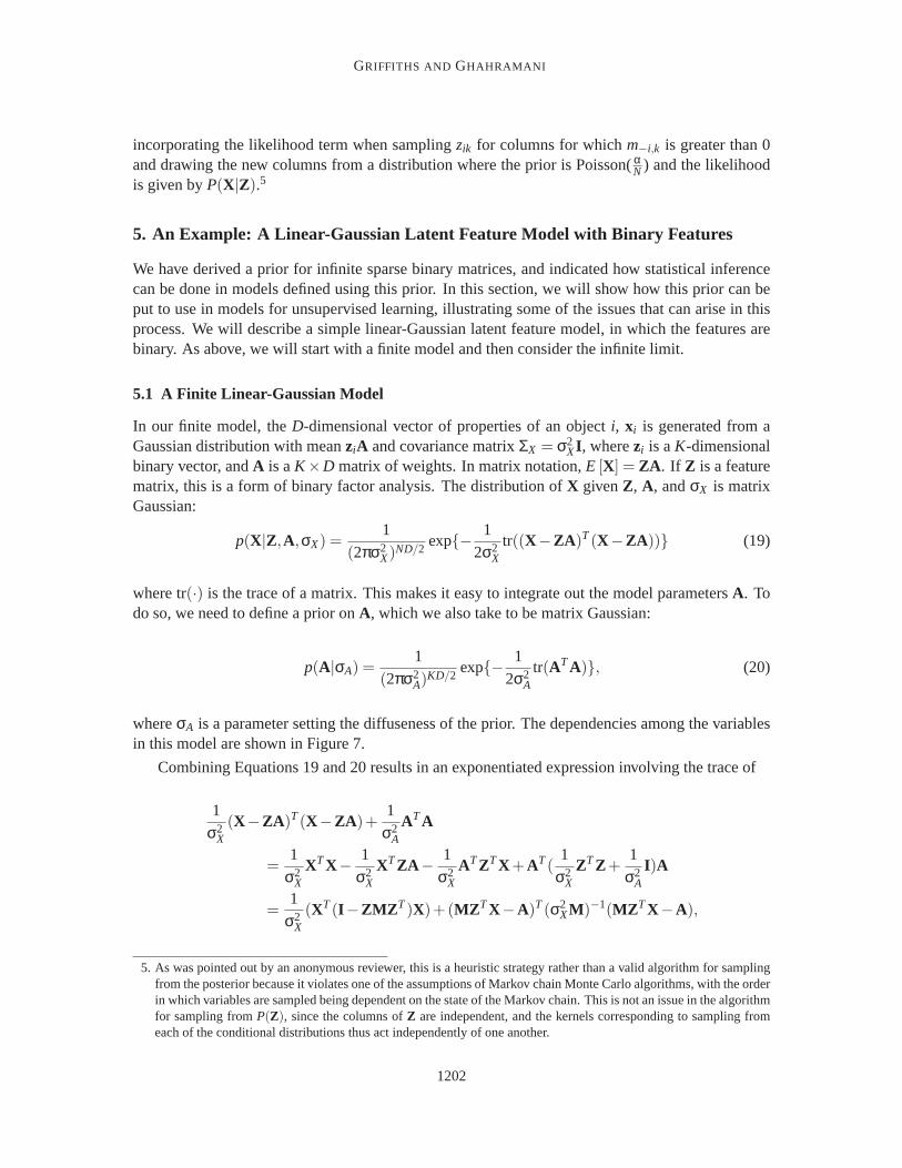
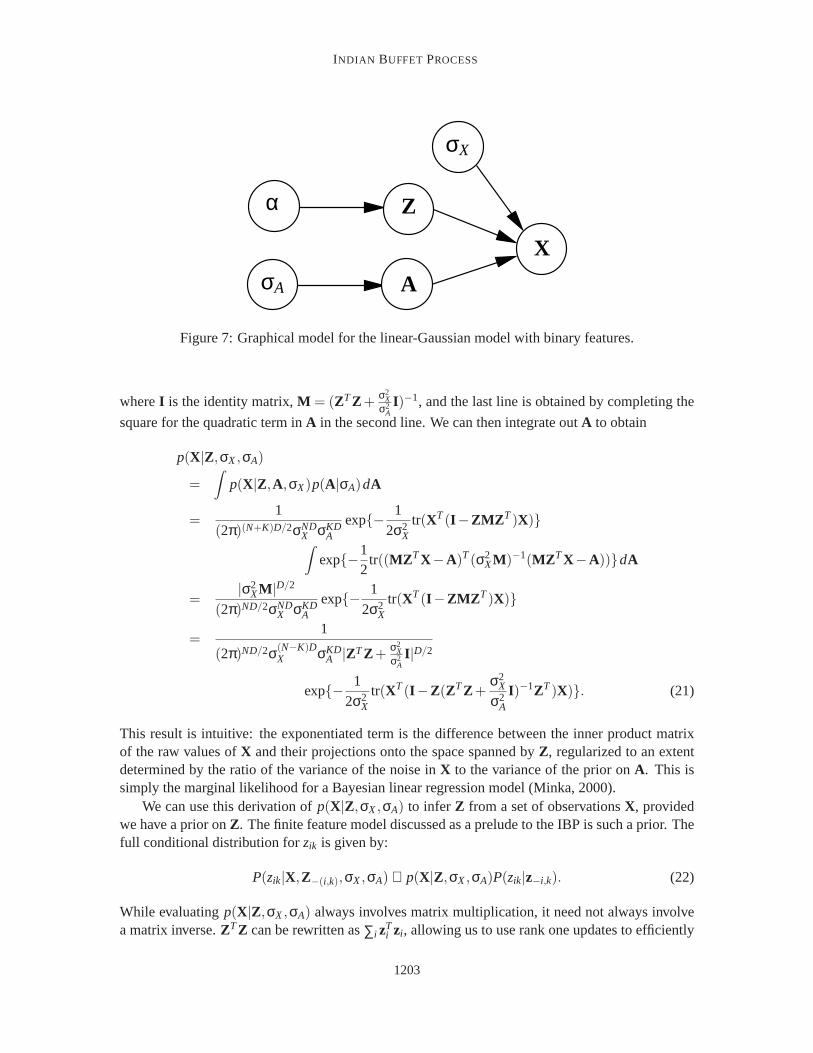
whereσA is a parameter setting the diffuseness of the prior. The dependencies among the variablesin this model are shown in Figure 7.
Combining Equations 19 and 20 results in an exponentiated expression involving the trace of
1
σ2X
(X−ZA)T(X−ZA)+1
σ2A
ATA
=1
σ2X
XTX−1
σ2X
XTZA −1
σ2X
ATZTX+AT(1
σ2X
ZTZ+1
σ2A
I)A
=1
σ2X
(XT(I −ZMZ T)X)+(MZ TX−A)T(σ2XM)−1(MZ TX−A),
5. As was pointed out by an anonymous reviewer, this is a heuristic strategy rather than a valid algorithm for samplingfrom the posterior because it violates one of the assumptions of Markov chain Monte Carlo algorithms, with the orderin which variables are sampled being dependent on the state of the Markovchain. This is not an issue in the algorithmfor sampling fromP(Z), since the columns ofZ are independent, and the kernels corresponding to sampling fromeach of the conditional distributions thus act independently of one another.
1202
INDIAN BUFFET PROCESS
Z
X
AσA
α
σX
Figure 7: Graphical model for the linear-Gaussian model with binary features.
whereI is the identity matrix,M = (ZTZ +σ2
Xσ2
AI)−1, and the last line is obtained by completing the
square for the quadratic term inA in the second line. We can then integrate outA to obtain
p(X|Z,σX,σA)
=∫
p(X|Z,A,σX)p(A|σA)dA
=1
(2π)(N+K)D/2σNDX σKD
A
exp{−1
2σ2X
tr(XT(I −ZMZ T)X)}
∫exp{−
12
tr((MZ TX−A)T(σ2XM)−1(MZ TX−A))}dA
=|σ2
XM |D/2
(2π)ND/2σNDX σKD
A
exp{−1
2σ2X
tr(XT(I −ZMZ T)X)}
=1
(2π)ND/2σ(N−K)DX σKD
A |ZTZ+σ2
Xσ2
AI |D/2
exp{−1
2σ2X
tr(XT(I −Z(ZTZ+σ2
X
σ2A
I)−1ZT)X)}. (21)
This result is intuitive: the exponentiated term is the difference between the inner product matrixof the raw values ofX and their projections onto the space spanned byZ, regularized to an extentdetermined by the ratio of the variance of the noise inX to the variance of the prior onA. This issimply the marginal likelihood for a Bayesian linear regression model (Minka,2000).
We can use this derivation ofp(X|Z,σX,σA) to infer Z from a set of observationsX, providedwe have a prior onZ. The finite feature model discussed as a prelude to the IBP is such a prior.Thefull conditional distribution forzik is given by:
P(zik|X,Z−(i,k),σX,σA) ∝ p(X|Z,σX,σA)P(zik|z−i,k). (22)
While evaluatingp(X|Z,σX,σA) always involves matrix multiplication, it need not always involvea matrix inverse.ZTZ can be rewritten as∑i z
Ti zi , allowing us to use rank one updates to efficiently
1203

GRIFFITHS AND GHAHRAMANI
compute the inverse when only onezi is modified. DefiningM−i = (∑ j 6=i zTj z j +
σ2X
σ2AI)−1, we have
M−i = (M−1−zTi zi)
−1
= M −MzT
i ziMziMzT
i −1, (23)
M = (M−1−i +zT
i zi)−1
= M−i −M−izT
i ziM−i
ziM−izTi +1
. (24)
Iteratively applying these updates allowsp(X|Z,σX,σA), to be computed via Equation 21 for dif-ferent values ofzik without requiring an excessive number of inverses, although a full rank updateshould be made occasionally to avoid accumulating numerical errors. The second part of Equation22,P(zik|z−i,k), can be evaluated using Equation 17.
5.2 Taking the Infinite Limit
To make sure that we can define an infinite version of this model, we need to check thatp(X|Z,σX,σA)remains well-defined ifZ has an unbounded number of columns.Z appears in two places in Equa-
tion 21: in|ZTZ+σ2
Xσ2
AI | and inZ(ZTZ+
σ2X
σ2AI)−1ZT . We will examine how these behave asK → ∞.
If Z is in left-ordered form, we can write it as[Z+ Z0], whereZ+ consists ofK+ columns withsumsmk > 0, andZ0 consists ofK0 columns with sumsmk = 0. It follows that the first of the twoexpressions we are concerned with reduces to
∣
∣
∣
∣
ZTZ+σ2
X
σ2A
I
∣
∣
∣
∣
=
∣
∣
∣
∣
[
ZT+Z+ 00 0
]
+σ2
X
σ2A
IK
∣
∣
∣
∣
=
(
σ2X
σ2A
)K0∣
∣
∣
∣
ZT+Z++
σ2X
σ2A
IK+
∣
∣
∣
∣
. (25)
The appearance ofK0 in this expression is not a problem, as we will see shortly. The abundance ofzeros inZ leads to a direct reduction of the second expression to
Z(ZTZ+σ2
X
σ2A
I)−1ZT = Z+(ZT+Z++
σ2X
σ2A
IK+)−1ZT
+,
which only uses the finite portion ofZ. Combining these results yields the likelihood for the infinitemodel
p(X|Z,σX,σA) =1
(2π)ND/2σ(N−K+)DX σK+D
A |ZT+Z++
σ2X
σ2AIK+ |
D/2
exp{−1
2σ2X
tr(XT(I −Z+(ZT+Z++
σ2X
σ2A
IK+)−1ZT
+)X)}. (26)
TheK+ in the exponents ofσA andσX appears as a result of introducingD/2 multiples of the factor
of(
σ2X
σ2A
)K0from Equation 25. The likelihood for the infinite model is thus just the likelihood for the
finite model defined on the firstK+ columns ofZ.
1204
INDIAN BUFFET PROCESS
The heuristic Gibbs sampling algorithm defined in Section 4.7 can now be used inthis model.Assignments to classes for whichm−i,k > 0 are drawn in the same way as for the finite model, viaEquation 22, using Equation 26 to obtainp(X|Z,σX,σA) and Equation 18 forP(zik|z−i,k). As inthe finite case, Equations 23 and 24 can be used to compute inverses efficiently. The distributionover the number of new features can be approximated by truncation, computing probabilities fora range of values ofK(i)
1 up to some reasonable upper bound. For each value,p(X|Z,σX,σA) canbe computed from Equation 26, and the prior on the number of new classes isPoisson(αN ). Moreelaborate samplers which do not require truncation are presented in Meeds et al. (2007) and in Tehet al. (2007).
5.3 Demonstrations
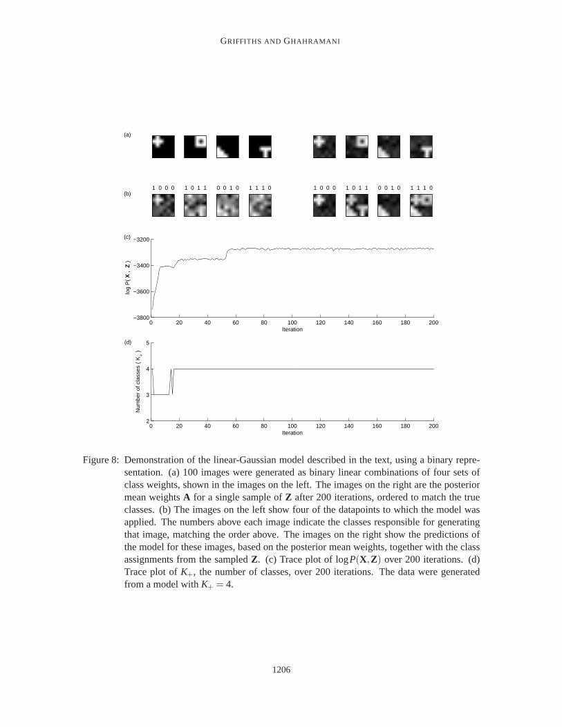
As a first demonstration of the ability of this algorithm to recover the latent structure responsiblefor having generated observed data, we applied the Gibbs sampler for theinfinite linear-Gaussianmodel to a simulated data set consisting of 100 6×6 images, each generated by randomly assigninga feature to each image to a class with probability 0.5, and taking a linear combination of theweights associated with features to which the images were assigned (a similar data set was used byGhahramani, 1995). Some of these images are shown in Figure 8, together with the weightsA thatwere used to generate them. The non-zero elements ofA were all equal to 1.0, andσX was set to0.5, introducing a large amount of noise.
The algorithm was initialized withK+ = 1, choosing the feature assignments for the first columnby settingzi1 = 1 with probability 0.5. σA was set to 1.0. The Gibbs sampler rapidly discoveredthat four classes were sufficient to account for the data, and converged to a distribution focused onmatricesZ that closely matched the true class assignments. The results are shown in Figure 8. Eachof the features is represented by the posterior mean of the feature weights, A, givenX andZ, whichis
E[A|X,Z] = (ZTZ+σ2
X
σ2A
I)−1ZTX.
for a single sampleZ. The results shown in the figure are from the 200th sample produced by thealgorithm.
These results indicate that the algorithm can recover the features used to generate simulateddata. In a further test of the algorithm with more realistic data, we applied it to a data set consistingof 100 240× 320 pixel images. We represented each image,xi , using a 100-dimensional vectorcorresponding to the weights of the mean image and the first 99 principal components. Each imagecontained up to four everyday objects—a $20 bill, a Klein bottle, a prehistorichandaxe, and acellular phone. The objects were placed in fixed locations, but were put into the scenes by hand,producing some small variation in location. The images were then taken with a low resolutionwebcam. Each object constituted a single latent feature responsible for theobserved pixel values.The images were generated by sampling a feature vector,zi , from a distribution under which eachfeature was present with probability 0.5, and then taking a photograph containing the appropriateobjects using a LogiTech digital webcam. Sample images are shown in Figure 9 (a). The only noisein the images was the noise from the camera.
The Gibbs sampler was initialized withK+ = 1, choosing the feature assignments for the firstcolumn by settingzi1 = 1 with probability 0.5. σA, σX, andα were initially set to 0.5, 1.7, and1 respectively, and then sampled by adding Metropolis steps to the MCMC algorithm. Figure 9
1205
GRIFFITHS AND GHAHRAMANI
1 0 0 0 1 0 1 1 0 0 1 0 1 1 1 0 1 0 0 0 1 0 1 1 0 0 1 0 1 1 1 0
0 20 40 60 80 100 120 140 160 180 200−3800
−3600
−3400
−3200
log
P(
X ,
Z )
Iteration
0 20 40 60 80 100 120 140 160 180 2002
3
4
5
Num
ber
of c
lass
es (
K+ )
Iteration
(a)
(b)
(c)
(d)
Figure 8: Demonstration of the linear-Gaussian model described in the text, using a binary repre-sentation. (a) 100 images were generated as binary linear combinations of four sets ofclass weights, shown in the images on the left. The images on the right are the posteriormean weightsA for a single sample ofZ after 200 iterations, ordered to match the trueclasses. (b) The images on the left show four of the datapoints to which the model wasapplied. The numbers above each image indicate the classes responsible for generatingthat image, matching the order above. The images on the right show the predictions ofthe model for these images, based on the posterior mean weights, together withthe classassignments from the sampledZ. (c) Trace plot of logP(X,Z) over 200 iterations. (d)Trace plot ofK+, the number of classes, over 200 iterations. The data were generatedfrom a model withK+ = 4.
1206
INDIAN BUFFET PROCESS
(a)
(Positive)
(b)
(Negative) (Negative) (Negative)
0 0 0 0
(c)
0 1 0 0 1 1 1 0 1 0 1 1
0 100 200 300 400 500 600 700 800 900 10000
5
10
K+
0 100 200 300 400 500 600 700 800 900 10000
2
4
α
0 100 200 300 400 500 600 700 800 900 10000
1
2
σ X
0 100 200 300 400 500 600 700 800 900 10000
1
2
σ A
Iteration
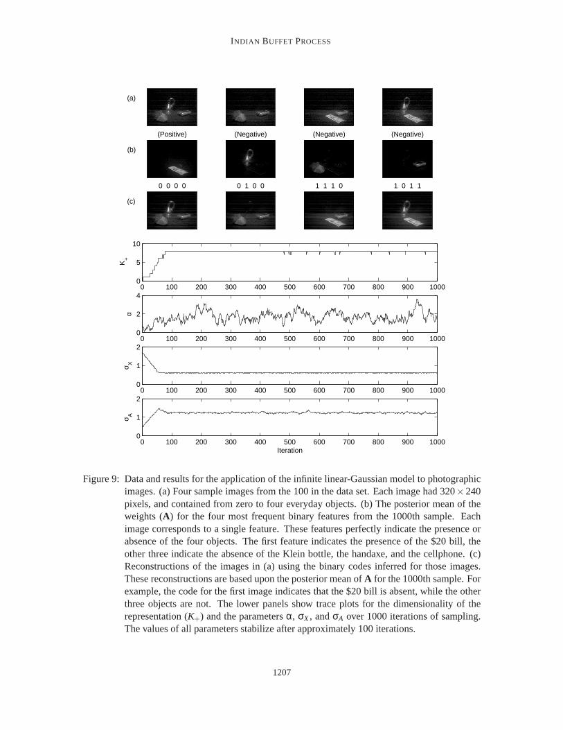
Figure 9: Data and results for the application of the infinite linear-Gaussian model to photographicimages. (a) Four sample images from the 100 in the data set. Each image had 320×240pixels, and contained from zero to four everyday objects. (b) The posterior mean of theweights (A) for the four most frequent binary features from the 1000th sample. Eachimage corresponds to a single feature. These features perfectly indicatethe presence orabsence of the four objects. The first feature indicates the presence of the $20 bill, theother three indicate the absence of the Klein bottle, the handaxe, and the cellphone. (c)Reconstructions of the images in (a) using the binary codes inferred for those images.These reconstructions are based upon the posterior mean ofA for the 1000th sample. Forexample, the code for the first image indicates that the $20 bill is absent, while the otherthree objects are not. The lower panels show trace plots for the dimensionalityof therepresentation (K+) and the parametersα, σX, andσA over 1000 iterations of sampling.The values of all parameters stabilize after approximately 100 iterations.
1207
GRIFFITHS AND GHAHRAMANI
shows trace plots for the first 1000 iterations of MCMC for the number of features used by at leastone object,K+, and the model parametersσA, σX, andα. All of these quantities stabilized afterapproximately 100 iterations, with the algorithm finding solutions with approximatelyseven latentfeatures.
Figure 9 (b) shows the posterior mean ofak for the four most frequent features in the 1000thsample produced by the algorithm. These features perfectly indicated presence and absence ofthe four objects. Three less common features coded for slight differences in the locations of thoseobjects. Figure 9 (c) shows the feature vectorszi from this sample for the four images in Figure 9(b),together with the posterior means of the reconstructions of these images for this sample,ziE[A|X,Z].Similar reconstructions are obtained by averaging over all values ofZ produced by the Markovchain. The reconstructions provided by the model clearly pick out the relevant content of the images,removing the camera noise in the original images.
These applications of the linear-Gaussian latent feature model are intended primarily to demon-strate that this nonparametric Bayesian approach can efficiently learn satisfying representationswithout requiring the dimensionality of those representations to be fixed a priori. The data setconsisting of images of objects was constructed in a way that removes many ofthe basic challengesof computer vision, with objects appearing in fixed orientations and locations.Dealing with theseissues requires using a more sophisticated image representation or a more complex likelihood func-tion than the linear-Gaussian model. Despite its simplicity, the example of identifying the objects inimages illustrates the kind of problems for which the IBP provides an appropriate prior. We describea range of other applications of the Indian buffet process in detail in the next section.
6. Further Applications and Alternative Inference Algorit hms
We now outline six applications of the Indian buffet process, each of which uses the same priorover infinite binary matrices,P(Z), but different choices for the likelihood relating such matrices toobserved data. These applications provide an indication of the potential uses of the IBP in machinelearning, and have also led to a number of alternative inference algorithms,which we will describebriefly.
6.1 Choice Behavior
Choice behavior refers to our ability to decide between several options. Models of choice behaviorare of interest to psychology, marketing, decision theory, and computer science. Our choices areoften governed by features of the different options. For example, when choosing which car to buy,one may be influenced by fuel efficiency, cost, size, make, etc. Gorur et al. (2006) present a non-parametric Bayesian model based on the IBP which, given the choice data,infers latent features ofthe options and the corresponding weights of these features. The likelihoodfunction is taken fromTversky’s (1972) classic “elimination by aspects” model of choice, with theprobability of choosingoptionA over optionB being proportional to the sum of the weights of the distinctive features ofA.The IBP is the prior over these latent features, which are assumed to be either present or absent.
The likelihood function used in this model does not have a natural conjugateprior, meaning thatthe approach taken in our Gibbs sampling algorithm—integrating out the parameters associated withthe features—cannot be used. This led Gorur et al. to develop a similar Markov chain Monte Carloalgorithm for use with a non-conjugate prior. The basic idea behind the algorithm is analogous toAlgorithm 8 of Neal (2000) for Dirichlet process mixture models, using a set of auxiliary variables
1208
INDIAN BUFFET PROCESS
to represent the weights associated with features that are currently not possessed by any of theavailable options. These auxiliary variables effectively provide a Monte Carlo approximation to thesum over parameters used in our Gibbs sampler (although there is no approximation error introducedthrough this step).
6.2 Modeling Protein Interactions
Proteomics aims to understand the functional interactions of proteins, and is afield of growingimportance to modern biology and medicine. One of the key concepts in proteomics is aproteincomplex, a group of several interacting proteins. Protein complexes can be experimentally deter-mined by doing high-throughput protein-protein interaction screens. Typically the results of suchexperiments are subjected to mixture-model based clustering methods. However, a protein can be-long to multiple complexes at the same time, making the mixture model assumption invalid. Chuet al. (2006) proposed a nonparametric Bayesian approach based onthe IBP for identifying proteincomplexes and their constituents from interaction screens. The latent binary featurezik indicateswhether proteini belongs to complexk. The likelihood function captures the probability that twoproteins will be observed to bind in the interaction screen as a function of how many complexes theyboth belong to,∑∞
k=1zikzjk. The approach automatically infers the number of significant complexesfrom the data and the results are validated using affinity purification/mass spectrometry experimen-tal data from yeast RNA-processing complexes.
6.3 Binary Matrix Factorization for Modeling Dyadic Data
Many interesting data sets aredyadic: there are two sets of objects or entities and observations aremade on pairs with one element from each set. For example, the two sets might consist of moviesand viewers, and the observations are ratings given by viewers to movies. Alternatively, the two setsmight be genes and biological tissues and the observations may be expression levels for particulargenes in different tissues. Dyadic data can often be represented as matrices and many modelsof dyadic data can be expressed in terms of matrix factorization. Models of dyadic data make itpossible to predict, for example, the ratings a viewer might give to a movie based on ratings fromother viewers, a task known ascollaborative filtering. A traditional approach to modeling dyadicdata isbi-clustering: simultaneously clustering both the rows (e.g., viewers) and the columns (e.g.,movies) of the observation matrix using coupled mixture models. However, as we have discussed,mixture models provide a very limited latent variable representation of data. Meeds et al. (2007)presented a more expressive model of dyadic data based on the two-parameter version of the Indianbuffet process. In this model, both movies and viewers are representedby binary latent vectorswith an unbounded number of elements, corresponding to the features theymight possess (e.g.,“likes horror movies”). The two corresponding infinite binary matrices interact via a real-valuedweight matrix which links features of movies to features of viewers, resultingin a binary matrixfactorization of the observed ratings.
The basic inference algorithm used in this model was similar to the non-conjugate version ofthe Gibbs sampler outlined above, but the authors also developed a number of novel Metropolis-Hastings proposals that are mixed with the steps of the Gibbs sampler. One proposal directly han-dles the number of new features associated with each object, facilitating one of the more difficultaspects of non-conjugate inference. Another proposal is a “split-merge” move, analogous to similarproposals used in models based on the CRP (Jain and Neal, 2004; Dahl, 2003). In contrast to the
1209
GRIFFITHS AND GHAHRAMANI
Gibbs sampler, which slowly affects the number of features used in the modelby changing a singlefeature allocation for a single object at a time, the split-merge proposal explores large-scale movessuch as dividing a single feature into two, or collapsing two features together. Combining theselarge-scale moves with the Gibbs sampler can result in a Markov chain Monte Carlo algorithm thatexplores the space of latent matrices faster.
6.4 Extracting Features from Similarity Judgments
One of the goals of cognitive psychology is to determine the kinds of representations that underliepeople’s judgments. In particular, theadditive clusteringmethod has been used to infer people’sbeliefs about the features of objects from their judgments of the similarity between them (Shepardand Arabie, 1979). Given a square matrix of judgments of the similarity between N objects, wheresi j is the similarity between objectsi and j, the additive clustering model seeks to recover aN×Kbinary feature matrixF and a vector ofK weights associated with those features such thatsi j ≈
∑Kk=1wk fik f jk. A standard problem for this approach is determining the value ofK, for which a
variety of heuristic methods have been used. Navarro and Griffiths (2007) presented a nonparametricBayesian solution to this problem, using the IBP to define a prior onF and assuming thatsi j hasa Gaussian distribution with mean∑K+
k=1wk fik f jk (following Tenenbaum, 1996). Using this methodprovides a posterior distribution over the effective dimension ofF, K+, and gives both a weight anda posterior probability for the presence of each feature.
Samples from the posterior distribution over feature matrices reveal some surprisingly rich rep-resentations expressed in classic similarity data sets. Performing posterior inference makes it possi-ble to discover that there are multiple sensible sets of features that could account for human similar-ity judgments, while previous approaches that had focused on finding the single best set of featuresmight only find one such set. For example, the nonparametric Bayesian modelreveals that people’ssimilarity judgments for numbers from 0-9 can be accounted for by a set of features that includesboth the odd and the even numbers, while previous additive clustering analyses (e.g., Tenenbaum,1996) had only produced the odd numbers.
The additive clustering model, like the choice model discussed above, is another case in whichnon-conjugate inference is necessary. In this case, the inference algorithm is rendered simpler bythe fact that no attempt is made to model the similarity of an object to itself,sii . As a consequence, afeature possessed by a single object has no effect on the likelihood, and the number of such featuresand their associated weights can be drawn directly from the prior. Inference thus proceeds using analgorithm similar to the Gibbs sampler derived above, with the addition of a Metropolis-Hastingsstep to update the weights associated with each feature.
6.5 Latent Features in Link Prediction
Network data, indicating the relationships among a group of people or objects, have been analyzedby both statisticians and sociologists. A basic goal of these analyses is predicting which unobservedrelationships might exist. For example, having observed friendly interactions among several pairsof people, a sociologist might seek to predict which other people are likely tobe friends with oneanother. This problem of link prediction can be solved using a probabilistic model for the structureof graphs. One popular class of models, known as stochastic blockmodels, assume that each entitybelongs to a single latent class, and that the probability of a relationship existing between two en-tities depends only on the classes of those entities (Nowicki and Snijders, 2001; Wang and Wong,
1210
INDIAN BUFFET PROCESS
1987). This is analogous to a mixture model, in which the probability that an object has certainobserved properties depends only on its latent class. Nonparametric versions of stochastic block-models can be defined using the Chinese restaurant process (Kemp et al.,2006), corresponding toan underlying stochastic process that generalizes the Dirichlet process(Roy and Teh, 2009).
Just as allowing objects to have latent features rather than a single latent class makes it possibleto go beyond mixture models, this approach allows us to define models for link prediction thatare richer than stochastic blockmodels. Miller et al. (2010) defined a classof nonparametric latentfeature models that can be used for link prediction. The key idea is to definethe probability of theexistence of a link between two entities in terms of a “squashing function” (such as the logistic orprobit) applied to a real-valued score for that link. The scores then depend on the features of thetwo entities. For a set ofN entities, the pairwise scores are given by theN×N matrix ZWZ T ,whereZ is a binary feature matrix, as used throughout this paper, andW is a matrix of real-valuedfeature weights. Since the feature weights can be positive or negative, features can interact to eitherincrease or decrease the probability of a link. The resulting model is strictly more expressive than astochastic blockmodel and produces more accurate predictions, particularly in cases where multiplefactors interact to influence the existence of a relationship (such as in the decision to co-author apaper, for example).
6.6 Independent Components Analysis and Sparse Factor Analysis
Independent Components Analysis (ICA) is a model which explains observed signals in terms of alinear superposition, or mixing, of independent hidden sources (Comon,1994; Bell and Sejnowski,1995; MacKay, 1996; Cardoso, 1998). ICA has been used to solve the problem of “blind sourceseparation” in which the goal is to unmix the hidden sources from the observed mixed signalswithout assuming much knowledge of the hidden source distribution. This models, for example, alistener in a cocktail party who may want to unmix the signals received on his twoears into the manyindependent sound sources that produced them. ICA is closely related tofactor analysis, except thatwhile in factor analysis the sources are assumed to be Gaussian distributed,in ICA the sources areassumed to have any distribution other than the Gaussian.
One of the key practical problems in ICA is determining the number of hidden sources. Knowlesand Ghahramani (2007) provided a solution to this problem by devising a non-parametric Bayesianmodel for ICA based on the IBP. The basic assumption of this ICA model is thatthe number ofpotential sources is unbounded, but that any particular source is typically not present in a givensignal. The IBP provides a natural model for determining which sources are present in each signal.In the notation of Section 3, the observed signals are represented by a matrix X, the presence orabsence of the hidden sources by the IBP distributed matrixZ, and the value taken by the sources bythe matrixV. Knowles and Ghahramani (2007) considered several variants of themodel, includingICA models where the elements ofV have Laplacian distributions, sparse FA models where theelements ofV have Gaussian distributions, and one and two parameter versions of the IBP in bothcases. The model was applied to discovering gene signatures from geneexpression microarray datafrom an ovarian cancer study.
Rai and Daume (2009) developed two interesting extensions of this model also motivated byapplications to gene expression data. First they considered both factor analysis and factor regressionmodels, where the latter refers to solving a regression problem with a typicallylarge number ofinput features by making predictions based solely on the factor representation. Second, they used
1211
GRIFFITHS AND GHAHRAMANI
an IBP to model the sparsity in the factor loading matrix (rather than the factor or source matrix innonparametric ICA) and they moreover assume that the factors are relatedto each other through ahierarchy. They used Kingman’s coalescent as a nonparametric Bayesian model for this hierarchy,following the inference algorithms developed in Teh et al. (2008). This paper shows a nice exampleof how the IBP can be integrated with other nonparametric Bayesian distributions in a fairly modularmanner to solve useful inference problems.
6.7 Bipartite Graphs and Learning Hidden Causes
Wood et al. (2006) used the IBP as part of an algorithm for learning the structure of graphicalmodels. Specifically, they focused on the case where an unknown numberof hidden variables (e.g.,diseases) are causes for some set of observed variables (e.g., symptoms). Rather than defining a priorover the number of hidden causes, Wood et al. used a non-parametric Bayesian approach based onthe IBP to model the structure of graphs with countably infinitely many hidden causes. The binaryvariablezik indicates whether hidden variablek has a direct causal influence on observed variablei; in other words whetherk is a parent ofi in the graph. The data being modeled were the valuesof the set of observed variables over a number of trials, where each variable was either present orabsent on each trial. Each hidden variable could be either present or absent on a particular trial, withthe probabilities of these states being determined by a parameter of the model, andhidden variableswere assumed to combine via a noisy-OR (Pearl, 1988) to influence the observed variables.
Wood et al. (2006) described an MCMC algorithm for inference in this model. Like many of thecases discussed in this section, this model lacked natural conjugate priors. Inference was done usinga variant on the Gibbs sampler introduced above, with additional steps to modify the values of thehidden variables. The sampling step for the introduction of new hidden causes into the graph wasfacilitated by an analytic result making it possible to sum out the values of the variables associatedwith those causes in a way that is analogous to summing out the parameters in a conjugate model.However, Wood and Griffiths (2007) developed a sequential Monte Carlo algorithm for use in thismodel, similar to algorithms that have been developed for use with the CRP (suchas Fearnhead,2004). This algorithm is a form of particle filter, updating the posterior distribution onZ one rowat a time (in this case, as new observed variables are added to the data). The particle filter providesan efficient and straightforward alternative for inference in models thatlack conjugate priors, andgeneralizes naturally to other models using the IBP.
6.8 Structuring Markov Transition Matrices
Discrete Markov processes are widely used in machine learning, as partof hidden Markov modelsand state-space models. Nonparametric Bayesian methods have been usedto define “infinite” ver-sions of these models, allowing the number of states in a hidden Markov model tobe unbounded(Beal et al., 2002). An infinite discrete Markov process can be definedby assuming that transitionsfrom each state follow a Chinese restaurant process, with transitions thathave been made frequentlyin the past being more likely in the future. When a new transition is generated, the next state isdrawn from a higher-level Chinese restaurant process that is shared across all states. The resultingdistribution can also be obtained from a hierarchical Dirichlet process (Teh et al., 2004).
Fox et al. (2010) recently explored another way of defining an infinite discrete Markov process,which allows for more structure in the transition matrix. In this model, it is assumed that each statecan only make transitions to a subset of other states. Thus, each state is associated with a binary
1212
INDIAN BUFFET PROCESS
vector indicating whether or not it makes transitions to other states. With an infinite set of states,a distribution over these vectors can be defined using the IBP. This approach was used to define anonparametric autoregressive hidden Markov model, in which a sequence of continuous variableswere predicted as a linear function of the variables at the previous timestep,but the parameters ofthe function were determined by a latent Markov process. The resulting model was able to identifymeaningful action components in motion capture data. In addition to introducing anovel model, thispaper explored the use of “birth and death” moves in the Markov chain Monte Carlo algorithm usedfor inference, in which entire columns of the matrix produced by the IBP were created or destroyed.
6.9 Other Inference Algorithms
The broad range of settings in which the IBP has been applied have encouraged the development ofmore efficient methods for probabilistic inference in the resulting nonparametric Bayesian models.As discussed above, several innovations have been used to speed mixing in the Markov chain MonteCarlo algorithms used with specific models. Other work has explored schemesfor making inferencein the linear-Gaussian model discussed in Section 5 more efficient and scalable to larger data sets.For example, if instead of integrating out the weight matrixA, the posterior distribution overA ismaintained, it is possible to use an alternative sampling scheme that still mixes quickly where thetime for each iteration scales linearly inN (Doshi-Velez and Ghahramani, 2009a). This observationalso provides the basis for a parallelization scheme in which the features of different objects arecomputed on different machines, with the potential to make large-scale applications of this linear-Gaussian model possible (Doshi-Velez et al., 2010). Similar principles may apply in the othermodels using the IBP discussed in this section.
An alternative approach to probabilistic inference is to reject the stochasticapproximations pro-vided by MCMC algorithms in favor of deterministic approximations, using variational inference toapproximate the posterior. A mean field approximation to the IBP was developedby Doshi-Velezet al. (2009), building on similar approximations for Dirichlet process mixturemodels (Blei andJordan, 2006). This variational inference method was applied to the infiniteICA model discussedin Section 6.6, and compared against sampling schemes on both synthetic and real data. The resultsof these comparisons suggested that the variational approach providesa more efficient strategy forinference in this model when the dimensionality of the observed data is high. Variational inferencemay thus be useful in working with some of the other models discussed in this section, at least inspecific regimes.
7. Extensions and Connections to Other Processes
The Indian buffet process gives a way to characterize our distributionon infinite binary matrices interms of a simple stochastic process. In this section we review how the IBP canbe extended to yieldmore general classes of distributions, and summarize some of the connections between the IBP andother stochastic processes. Our derivation of the IBP was based on considering the infinite limitof a distribution on finite binary matrices. As with the CRP, this distribution can alsobe derivedvia a stick-breaking construction, or by marginalizing out an underlying measure. These differentviews of the IBP yield different generalizations of the distribution, and different opportunities fordeveloping inference algorithms.
1213
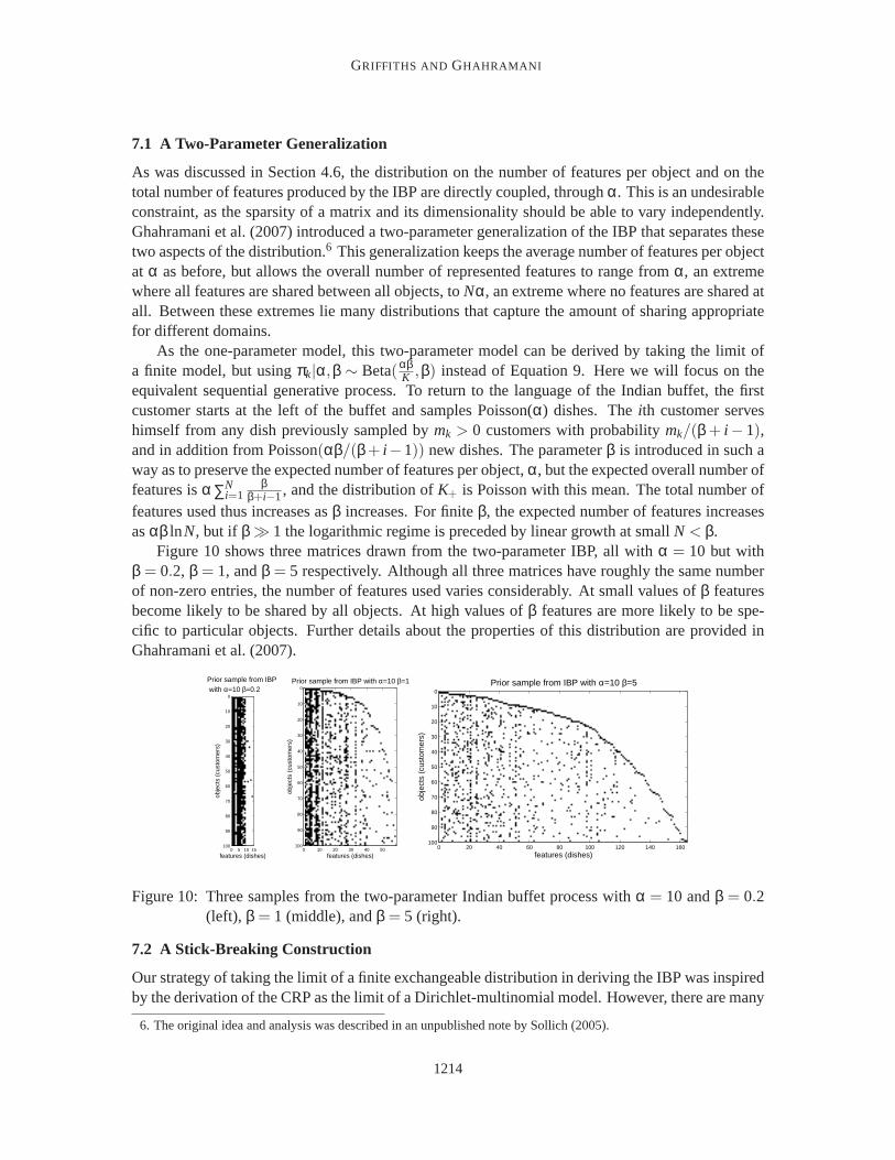
GRIFFITHS AND GHAHRAMANI
7.1 A Two-Parameter Generalization
As was discussed in Section 4.6, the distribution on the number of features per object and on thetotal number of features produced by the IBP are directly coupled, throughα. This is an undesirableconstraint, as the sparsity of a matrix and its dimensionality should be able to varyindependently.Ghahramani et al. (2007) introduced a two-parameter generalization of the IBP that separates thesetwo aspects of the distribution.6 This generalization keeps the average number of features per objectat α as before, but allows the overall number of represented features to range fromα, an extremewhere all features are shared between all objects, toNα, an extreme where no features are shared atall. Between these extremes lie many distributions that capture the amount of sharing appropriatefor different domains.
As the one-parameter model, this two-parameter model can be derived by taking the limit ofa finite model, but usingπk|α,β ∼ Beta(αβ
K ,β) instead of Equation 9. Here we will focus on theequivalent sequential generative process. To return to the languageof the Indian buffet, the firstcustomer starts at the left of the buffet and samples Poisson(α) dishes. Theith customer serveshimself from any dish previously sampled bymk > 0 customers with probabilitymk/(β+ i − 1),and in addition from Poisson(αβ/(β+ i −1)) new dishes. The parameterβ is introduced in such away as to preserve the expected number of features per object,α, but the expected overall number offeatures isα∑N
i=1β
β+i−1, and the distribution ofK+ is Poisson with this mean. The total number offeatures used thus increases asβ increases. For finiteβ, the expected number of features increasesasαβ lnN, but if β ≫ 1 the logarithmic regime is preceded by linear growth at smallN < β.
Figure 10 shows three matrices drawn from the two-parameter IBP, all withα = 10 but withβ = 0.2, β = 1, andβ = 5 respectively. Although all three matrices have roughly the same numberof non-zero entries, the number of features used varies considerably. At small values ofβ featuresbecome likely to be shared by all objects. At high values ofβ features are more likely to be spe-cific to particular objects. Further details about the properties of this distribution are provided inGhahramani et al. (2007).
obje
cts
(cus
tom
ers)
features (dishes)
Prior sample from IBP with α=10 β=0.2
0 5 10 15
0
10
20
30
40
50
60
70
80
90
100
obje
cts
(cus
tom
ers)
features (dishes)
Prior sample from IBP with α=10 β=1
0 10 20 30 40 50
0
10
20
30
40
50
60
70
80
90
100
obje
cts
(cus
tom
ers)
features (dishes)
Prior sample from IBP with α=10 β=5
0 20 40 60 80 100 120 140 160
0
10
20
30
40
50
60
70
80
90
100
Figure 10: Three samples from the two-parameter Indian buffet process with α = 10 andβ = 0.2(left), β = 1 (middle), andβ = 5 (right).
7.2 A Stick-Breaking Construction
Our strategy of taking the limit of a finite exchangeable distribution in deriving the IBP was inspiredby the derivation of the CRP as the limit of a Dirichlet-multinomial model. However, there are many
6. The original idea and analysis was described in an unpublished note bySollich (2005).
1214
INDIAN BUFFET PROCESS
other routes by which the CRP can be derived. One of these is via the Dirichlet process (Ferguson,1973). A simple way to think about the Dirichlet process is in terms of a probability measure overprobability measures. The parameters of the process are its concentrationα and a base measureG0. In a typical use, we would draw a measureG from the Dirichlet process, and then generateparameters for a modelφi by sampling them independently fromG. Since the Dirichlet processgenerates discrete measures with probability 1, it is possible for multiple parameters φi and φ j
drawn fromG to take the same value. We can thus imagine indexing the values taken by theφi withdiscrete variableszi , such thatzi = zj if and only if φi = φ j . Thezi thus index unique values ofφi ,and correspond to a partition of the indices of theφi . The distribution over partitionsz produced bythe Dirichlet process, integrating overG, is the CRP (Blackwell and MacQueen, 1973).
A straightforward way to understand how the Dirichlet process allocates probabilities to a dis-crete set of atoms is to think about assigning probabilities in terms of breaking off pieces of a stick.The stick is one unit in length, corresponding to the fact that our probabilities must sum to one.Each piece of stick we break off represents the probability assigned to another discrete atom. Afterbreaking off each piece, we then consider how much of the remainder to break off as the next piece.Sethuraman (1994) showed that if this process is repeated infinitely often,with a proportion of thestick drawn from a Beta(α,1) distribution being broken off at each step, the lengths of the piecesof broken stick are equivalent to the probabilities assigned to a discrete set of atoms by the Dirich-let process with parameterα. This stick-breaking representation of the Dirichlet process is usefulin deriving its properties, and in developing inference algorithms such as the variational inferencealgorithm proposed by Blei and Jordan (2006).
Teh et al. (2007) showed that a similar stick-breaking construction can bedefined for the IBP.First, we imagine sorting theπk representing the probability of each feature being possessed byan object from largest to smallest. Then, if we consider the proportion of the stick that is brokenoff and discarded at each break in the stick-breaking construction forthe Dirichlet process, thedistribution of the sequence of stick lengths corresponds exactly to the distribution of these orderedprobabilities. This stick-breaking construction identifies an interesting relationship between the IBPand the Dirichlet process, and is useful for exactly the same reasons. In particular, the stick-breakingconstruction was used in defining the variational inference algorithm summarized in Section 6.9, andcan also be used to derive other inference algorithms for the IBP, such as slice sampling (Teh et al.,2007).
7.3 Connections to the Beta Process
The relationship between the CRP and the Dirichlet process is an instance ofa more general re-lationship between exchangeable distributions and underlying probability measures. The resultssummarized in the previous paragraph indicate that we can write
P(z) =∫ N
∏i=1
P(zi |G)p(G)dG,
where thezi are drawn independently from the measureG, which is generated from the Dirichletprocess. The fact that we can represent the exchangeable distribution P(z) as the result of generatingthezi independently from a latent measure is a specific instance of the more general principle statedin de Finetti’s exchangeability theorem, which indicates thatanyexchangeable distribution can berepresented in this way (see Bernardo and Smith, 1994, for details). Thisraises a natural question:is there a similar measure underlying the exchangeable distribution producedby the IBP?
1215
GRIFFITHS AND GHAHRAMANI
Thibaux and Jordan (2007) provided an answer to this question, showing that the exchangeabledistribution produced by the IBP corresponds to the use of a latent measure based on the beta process(Hjort, 1990). The beta process provides a source of Bernoulli parametersπk associated with theelements of a (possibly continuous) index set. Sampling each of thezik independently accordingto the distribution defined by the appropriate parameter results in the same distribution on Z asthe IBP. This perspective also makes it straightforward to define analogues of the two-parameterprocess described in Section 7.1, and to extend the IBP to a hierarchical model that can capturecorrelations in the features exhibited in multiple data sets. Teh and Gorur (2010) also recentlyused the relationship to the beta process to define a variant of the IBP that produces a power-lawdistribution in feature frequencies, exploiting a connection to stable processes. Variants of this kindmay be useful in settings where power-law distributions are common, such asnatural languageprocessing.
7.4 Relaxing the Assumption of Exchangeability
The IBP assumes independence between the columns ofZ, and only the kind of weak dependencyimplied by exchangeability for the rows ofZ. Both of these assumptions have been relaxed in sub-sequent work. Producing correlations between the columns ofZ can be done by supplementing theIBP with a secondary process capturing patterns in the latent features (Doshi-Velez and Ghahramani,2009b). Modifying the assumption of exchangeability is potentially more problematic. Exchange-ability was one of our original desiderata, since it is a reasonable assumption in many settings andsimplifies probabilistic inference. However, this assumption is not warrantedin cases where wehave additional information about the properties of our observations, such as the fact that they wereproduced in a particular temporal sequence, or reflect a known patternof correlation. The chal-lenge is thus to identify how the assumption of exchangeability can be relaxed while maintainingthe tractability of probabilistic inference. Two recent papers have presented strategies for modifyingthe IBP to capture different forms of dependency between the rows ofZ.
The first kind of dependency can arise as the consequence of observations being generated in aspecific sequence. In such a case, it might be appropriate to assume thatthe latent features associatedwith observations made closer in time should be more correlated. A strategy formodifying the IBPto capture this kind of dependency was introduced by Van Gael et al. (2009). In this model—theMarkov Indian buffet process—it is assumed that the rows ofZ are generated via a Markov process,where the values in each column are generated based on the corresponding values in the previousrow. This Markov process has two parameters, giving the probability of a0 in the previous rowchanging to a 1, and the probability of a 1 in the previous row remaining unchanged. By assumingthat these parameters are generated from a Beta distribution and taking a limit analogous to that usedin the derivation of the IBP, it is possible to define a distribution over equivalence classes of binarymatrices in which the rows of the matrix reflect a Markov dependency structure. This model can beused to define richer nonparametric models for temporal data, such as an infinite factorial hiddenMarkov model, and probabilistic inference can be carried out using a slicesampler (see Van Gaelet al., 2009, for details).
A second kind of dependency can be the result of known degrees of relatedness among observa-tions. For example, one might seek to draw inferences about a group of people with known geneticrelationships, or about a set of organisms or languages with a known evolutionary history. In caseswhere the degrees of relatedness can be expressed in a tree, the phylogenetic Indian buffet process
1216
INDIAN BUFFET PROCESS
(Miller et al., 2008) can be used. In this model, the tree expresses the dependency structure thatgoverns the rows ofZ, and each column is generated independently by sampling from a stochasticprocess defined on the tree. The parameters of the stochastic process are specified in a way thatguarantees the total number of columns follows a Poisson distribution, and theoriginal IBP is re-covered as the special case where the tree is degenerate, with all branches meeting at the root. Treescan be used to capture a wide range of dependency structures, including partial exchangeability, andprobabilistic inference by MCMC remains tractable because belief propagation on the tree can beused to efficiently compute the relevant conditional probabilities.
8. Conclusions and Future Work
The methods that have been used to define infinite latent class models can be extended to models inwhich objects are represented in terms of a set of latent features, and used to derive distributions oninfinite binary matrices that can be used as priors for such models. We usedthis method to derive aprior that is the infinite limit of a simple distribution on finite binary matrices, and showed that thesame distribution can be specified in terms of a simple stochastic process—the Indian buffet process.This distribution satisfies our two desiderata for a prior for infinite latent feature models: objectsare exchangeable, and inference remains tractable. When used as a prior in models that representobjects using latent features, this distribution can be used to automatically inferthe number offeatures required to account for observed data. More generally, it can be used as a prior in anysetting where a sparse binary matrix with a finite number of rows and infinite number of columns isappropriate, such as estimating the adjacency matrix of a bipartite graph where the size of one classof nodes is unknown.
Recent work has made significant progress on turning this nonparametricapproach to inferringlatent features into a tool that can be used to solve a wide range of machine learning problems. Theseadvances include more sophisticated MCMC algorithms, schemes for parallelizing probabilisticinference, and deterministic methods for approximating posterior distributionsover latent featurematrices. The connections between the IBP and other stochastic processes provide the groundworkfor further understanding and extending this class of probabilistic models,making it possible tomodify the distribution over feature assignments and to capture different patterns of dependencythat might exist among the latent features of objects. As with the CRP, the different views of theIBP that result from considering the stick-breaking construction or the underlying measure that ismarginalized out to obtain the combinatorial stochastic process each support different extensions,generalizations, and inference algorithms.
Despite the wide array of successful applications of the IBP and related distributions, we viewone of the primary contributions of this work to be the idea that we can define richer nonparametricBayesian models to suit the unique challenges of machine learning. Our success in transferringthe strategy of taking the limit of a finite model from latent classes to latent features suggests thatthe same strategy might be applied with other representations, broadening thekinds of latent struc-ture that can be recovered through unsupervised learning. This idea receives support both fromother examples of new nonparametric models defined via a similar strategy (e.g.,Titsias, 2008),and from theoretical analyses of the conditions under which infinite models remain well definedwhen obtained as limits of finite models (Orbanz, 2010). We anticipate that therewill be othercombinatorial structures for which this strategy will result in new and useful distributions.
1217
GRIFFITHS AND GHAHRAMANI
Acknowledgments
This work was presented at the Neural Information Processing Systems conference, and draws onthe conference paper (Griffiths and Ghahramani, 2006) and associated technical report (Griffithsand Ghahramani, 2005). The preparation of this article was supported bygrants BCS-0631518 andIIS-0845410 from the National Science Foundation, and grant FA-9550-10-1-0232 from the AirForce Office of Scientific Research. We thank three anonymous reviewers for their comments onthe manuscript.
Appendix A. Details of Limits
This appendix contains the details of the limits of three expressions that appear in Equations 5 and14.
The first expression is
K!K0! KK+
=∏K+
k=1(K−k+1)
KK+
=KK+ − (K+−1)K+
2 KK+−1+ · · ·+(−1)K+−1(K+−1)!K
KK+
= 1−(K+−1)K+
2K+ · · ·+
(−1)K+−1(K+−1)!KK+−1 .
For finiteK+, all terms except the first go to zero asK → ∞.The second expression is
mk−1
∏j=1
( j + αK ) = (mk−1)!+ α
K
mk−1
∑j=1
(mk−1)!j
+ · · ·+( α
K
)mk−1.
For finitemk andα, all terms except the first go to zero asK → ∞.The third expression is
(
N!
∏Nj=1( j + α
K )
)K
=
(
∏Nj=1 j
∏Nj=1( j + α
K )
)K
=
(
N
∏j=1
j( j + α
K )
)K
=N
∏j=1
1
1+α 1
j
K
K
. (27)
We can now use the fact that
limK→∞
(
11+ x
K
)K
= exp{−x}
1218
INDIAN BUFFET PROCESS
to compute the limit of Equation 27 asK → ∞, obtaining
limK→∞
N
∏j=1
1
1+α 1
j
K
K
=N
∏j=1
exp{−α1j }
= exp{−αN
∑j=1
1j }
= exp{−αHN},
as desired.
References
D. Aldous. Exchangeability and related topics. InEcole d’ete de probabilites de Saint-Flour, XIII—1983, pages 1–198. Springer, Berlin, 1985.
C. Antoniak. Mixtures of Dirichlet processes with applications to Bayesian nonparametric prob-lems.The Annals of Statistics, 2:1152–1174, 1974.
M. J. Beal, Z. Ghahramani, and C. E. Rasmussen. The infinite hidden Markov model. MachineLearning, pages 29–245, 2002.
A. J. Bell and T. J. Sejnowski. An information maximisation approach to blind separation and blinddeconv olution.Neural Computation, 7(6):1129–1159, 1995.
J. M. Bernardo and A. F. M. Smith.Bayesian Theory. Wiley, New York, 1994.
D. Blackwell and J. MacQueen. Ferguson distributions via Polya urn schemes. The Annals ofStatistics, 1:353–355, 1973.
D. Blei and M. Jordan. Variational inference for Dirichlet process mixtures. Journal of BayesianAnalysis, 1:121–144, 2006.
D. Blei, T. Griffiths, M. Jordan, and J. Tenenbaum. Hierarchical topic models and the nested Chi-nese restaurant process. InAdvances in Neural Information Processing Systems 16. MIT Press,Cambridge, MA, 2004.
C. A. Bush and S. N. MacEachern. A semi-parametric Bayesian model for randomized blockdesigns.Biometrika, 83:275–286, 1996.
J.-F. Cardoso. Blind signal separation: statistical principles.Proceedings of the IEEE, 86(10):2009–2025, Oct 1998.
W. Chu, Z. Ghahramani, R. Krause, and D. L. Wild. Identifying protein complexes in high-throughput protein interaction screens using an infinite latent feature model.In BIOCOMPUTING2006: Proceedings of the Pacific Symposium, volume 11, pages 231–242, 2006.
P. Comon. Independent component analysis: A new concept.Signal Processing, 36:287–314, 1994.
1219
GRIFFITHS AND GHAHRAMANI
D. B. Dahl. An improved merge-split sampler for conjugate Dirichlet process mixture models.Technical Report 1086, Department of Statistics, University of Wisconsin, 2003.
A. d’Aspremont, L. El Ghaoui, I. Jordan, and G. R. G. Lanckriet. A direct formulation for sparsePCA using semidefinite programming. Technical Report UCB/CSD-04-1330, Computer ScienceDivision, University of California, Berkeley, 2004.
F. Doshi-Velez and Z. Ghahramani. Accelerated Sampling for the Indian Buffet Process. InInter-national Conference on Machine Learning (ICML 2009), 2009a.
F. Doshi-Velez and Z. Ghahramani. Correlated non-parametric latent feature models. InProceedingsof the Proceedings of the Twenty-Fifth Conference Annual Conference on Uncertainty in ArtificialIntelligence (UAI-09), pages 143–150, 2009b.
F. Doshi-Velez, K.T. Miller, J. Van Gael, and Y.W. Teh. Variational Inference for the Indian BuffetProcess. InArtificial Intelligence and Statistics Conference (AISTATS 2009), 2009.
F. Doshi-Velez, D. Knowles, S. Mohamed, and Z. Ghahramani. Large scale nonparametric Bayesianinference: Data parallelisation in the Indian buffet process. InAdvances in Neural InformationProcessing Systems 22, 2010.
M. D. Escobar and M. West. Bayesian density estimation and inference using mixtures.Journal ofthe American Statistical Association, 90:577–588, 1995.
P. Fearnhead. Particle filters for mixture models with an unknown number of components.Statisticsand Computing, 14:11–21, 2004.
T. Ferguson. A Bayesian analysis of some nonparametric problems.The Annals of Statistics, 1:209–230, 1973.
T. S. Ferguson. Bayesian density estimation by mixtures of normal distributions. In M. Rizvi,J. Rustagi, and D. Siegmund, editors,Recent Advances in Statistics, pages 287–302. AcademicPress, New York, 1983.
E. B. Fox, E. B. Sudderth, M. I. Jordan, and A. S. Willsky. Sharing features among dynamicalsystems with beta processes. InAdvances in Neural Information Processing Systems 22, 2010.
S. Geman and D. Geman. Stochastic relaxation, Gibbs distributions, and the Bayesian restorationof images.IEEE Transactions on Pattern Analysis and Machine Intelligence, 6:721–741, 1984.
Z. Ghahramani. Factorial learning and the EM algorithm. InAdvances in Neural InformationProcessing Systems 7. Morgan Kaufmann, San Francisco, CA, 1995.
Z. Ghahramani, T. L. Griffiths, and P. Sollich. Bayesian nonparametric latent feature models. InBayesian Statistics 8. Oxford University Press, Oxford, 2007.
W.R. Gilks, S. Richardson, and D. J. Spiegelhalter, editors.Markov Chain Monte Carlo in Practice.Chapman and Hall, Suffolk, UK, 1996.
1220
INDIAN BUFFET PROCESS
D. Gorur, F. Jakel, and C. E. Rasmussen. A choice model with infinitely many latent features.In Proceedings of the 23rd International Conference on Machine Learning (ICML 2006), pages361–368, New York, 2006. ACM Press.
P. Green and S. Richardson. Modelling heterogeneity with and without the Dirichlet process.Scan-dinavian Journal of Statistics, 28:355–377, 2001.
T. L. Griffiths and Z. Ghahramani. Infinite latent feature models and the Indian buffet process.Technical Report 2005-001, Gatsby Computational Neuroscience Unit,2005.
T. L. Griffiths and Z. Ghahramani. Infinite latent feature models and the Indian buffet process. InAdvances in Neural Information Processing Systems 18, Cambridge, MA, 2006. MIT Press.
K. A. Heller and Z. Ghahramani. Bayesian hierarchical clustering. InInternational Conference onMachine Learning (ICML 2005), 2005.
N. L. Hjort. Nonparametric Bayes estimators based on Beta processes in models for life historydata.Annals of Statistics, 18:1259–1294, 1990.
H. Ishwaran and L. F. James. Gibbs sampling methods for stick-breaking priors. Journal of theAmerican Statistical Association, 96:1316–1332, 2001.
S. Jain and R. M. Neal. A split-merge Markov chain Monte Carlo procedurefor the DirichletProcess mixture model.Journal of Computational and Graphical Statistics, 13:158–182, 2004.
I. T. Jolliffe. Principal component analysis. Springer, New York, 1986.
I. T. Jolliffe and M. Uddin. A modified principal component technique based on the lasso.Journalof Computational and Graphical Statistics, 12:531–547, 2003.
C. Kemp, J. B. Tenenbaum, T. L. Griffiths, T. Yamada, and N. Ueda. Learning systems of conceptswith an infinite relational model. InProceedings of the 21st National Conference on ArtificialIntelligence, 2006.
D. Knowles and Z. Ghahramani. Infinite sparse factor analysis and infiniteindependent compo-nents analysis. In7th International Conference on Independent Component Analysis and SignalSeparation (ICA 2007), Lecture Notes in Computer Science Series (LNCS). Springer, 2007.
D. J. C. MacKay. Maximum likelihood and covariant algorithms for independent component anal-ysis. Technical Report Draft 3.7, Cavendish Laboratory, University of Cambridge, MadingleyRoad, Cambridge CB3 0HE, December 1996.
E. Meeds, Z. Ghahramani, R. Neal, and S. T. Roweis. Modeling dyadic data with binary latentfactors. In B. Scholkopf, J. Platt, and T. Hoffman, editors,Advances in Neural InformationProcessing Systems, Cambridge, MA, 2007. MIT Press.
K. T. Miller, T. L. Griffiths, and M. I. Jordan. The phylogenetic Indian buffet process: A non-exchangeable nonparametric prior for latent features. InProceedings of the Twenty-Fourth Con-ference on Uncertainty in Artificial Intelligence (UAI 2008), 2008.
1221

GRIFFITHS AND GHAHRAMANI
K. T. Miller, T. L. Griffiths, and M. I. Jordan. Nonparametric latent feature models for link predic-tions. InAdvances in Neural Information Processing Systems 22, 2010.
T. Minka. Bayesian linear regression. Technical report, MIT Media Lab, 2000.http://research.microsoft.com/en-us/um/people/minka/papers/linear.html.
D. J. Navarro and T. L. Griffiths. A nonparametric Bayesian model for inferring features fromsimilarity judgments. In B. Scholkopf, J. Platt, and T. Hoffman, editors,Advances in NeuralInformation Processing Systems 19, Cambridge, MA, 2007. MIT Press.
R. M. Neal. Bayesian mixture modeling. InMaximum Entropy and Bayesian Methods: Proceedingsof the 11th International Workshop on Maximum Entropy and Bayesian Methods of StatisticalAnalysis, pages 197–211. Kluwer, Dordrecht, 1992.
R. M. Neal. Markov chain sampling methods for Dirichlet process mixture models. Journal ofComputational and Graphical Statistics, 9:249–265, 2000.
R. M. Neal. Density modeling and clustering using dirichlet diffusion trees. In J. M. Bernardo et al.,editor,Bayesian Statistics 7, pages 619–629, 2003.
K. Nowicki and T. A. B. Snijders. Estimation and prediction for stochastic blockstructures.Journalof the American Statistical Association, 96:1077–1087, 2001.
P. Orbanz. Construction of nonparametric Bayesian models from parametric Bayes equations. InAdvances in Neural Information Processing Systems 22, 2010.
J. Pearl.Probabilistic Reasoning in Intelligent Systems. Morgan Kaufmann, San Francisco, CA,1988.
J. Pitman. Combinatorial stochastic processes, 2002. Notes for Saint Flour Summer School.
P. Rai and H. Daume. The infinite hierarchical factor regression model. InAdvances in NeuralInformation Processing Systems, volume 21, 2009.
C. Rasmussen. The infinite Gaussian mixture model. InAdvances in Neural Information ProcessingSystems 12. MIT Press, Cambridge, MA, 2000.
C. E. Rasmussen and Z. Ghahramani. Occam’s razor. InAdvances in Neural Information ProcessingSystems 13. MIT Press, Cambridge, MA, 2001.
S. Roweis and Z. Ghahramani. A unifying review of linear Gaussian models.Neural Computation,11:305–345, 1999.
D. M. Roy and Y. W. Teh. The mondrian process. InAdvances in Neural Information ProcessingSystems 21, 2009.
J. Sethuraman. A constructive definition of Dirichlet priors.Statistica Sinica, 4:639–650, 1994.
R. Shepard and P. Arabie. Additive clutering: Representation of similaritiesas combinations ofdiscrete overlapping properties.Psychological Review, 86:87–123, 1979.
1222
INDIAN BUFFET PROCESS
P. Sollich. Indian buffet process with tunable feature repulsion, 2005.
E. Sudderth, A. Torralba, W. Freeman, and A. Willsky. Describing visual scenes using transformedDirichlet processes. InAdvances in Neural Information Processing Systems 18, Cambridge, MA,2006. MIT Press.
Y. Teh, M. Jordan, M. Beal, and D. Blei. Hierarchical Dirichlet processes. InAdvances in NeuralInformation Processing Systems 17. MIT Press, Cambridge, MA, 2004.
Y. W. Teh and D. Gorur. Indian buffet processes with power-law behavior. InAdvances in NeuralInformation Processing Systems 22, 2010.
Y. W. Teh, D. Gorur, and Z. Ghahramani. Stick-breaking construction for the Indian buffet process.In Eleventh International Conference on Artificial Intelligence and Statistics (AISTATS 2007),San Juan, Puerto Rico, 2007.
Y. W. Teh, H. Daume, and D. M. Roy. Bayesian agglomerative clustering with coalescents. InAdvances in Neural Information Processing Systems, volume 20, 2008.
J. B. Tenenbaum. Learning the structure of similarity. In D. S. Touretzky,M. C. Mozer, and M. E.Hasselmo, editors,Advances in neural information processing systems 8, pages 3–9. MIT Press,Cambridge, MA, 1996.
R. Thibaux and M. I. Jordan. Hierarchical Beta processes and the Indian buffet process. InEleventhInternational Conference on Artificial Intelligence and Statistics (AISTATS2007), 2007.
M. E. Tipping and C. M. Bishop. Probabilistic principal component analysis. Journal of the RoyalStatistical Society, Series B, 61:611–622, 1999.
M. Titsias. The infinite gamma-poisson feature model. In J.C. Platt, D. Koller, Y.Singer, andS. Roweis, editors,Advances in Neural Information Processing Systems 20. MIT Press, Cam-bridge, MA, 2008.
A. Tversky. Elimination by aspects: A theory of choice.Psychological Review, 79:281–299, 1972.
N. Ueda and K. Saito. Parametric mixture models for multi-labeled text. InAdvances in NeuralInformation Processing Systems 15, Cambridge, 2003. MIT Press.
J. Van Gael, Y.W. Teh, and Z. Ghahramani. The infinite factorial hidden Markov model. InAdvancesin Neural Information Processing Systems, volume 21, 2009.
Y. J. Wang and G. Y. Wong. Stochastic blockmodels for directed graphs.Journal of the AmericanStatistical Association, 82:8–19, 1987.
M. West, P. Muller, and M. Escobar. Hierarchical priors and mixture models, with application inregression and density estimation. In P. Freeman and A. Smith, editors,Aspects of Uncertainty,pages 363–386. Wiley, New York, 1994.
F. Wood and T. L. Griffiths. Particle filtering for nonparametric Bayesian matrix factorization.In B. Scholkopf, J. Platt, and T. Hoffman, editors,Advances in Neural Information ProcessingSystems 19, pages 1513–1520. MIT Press, Cambridge, MA, 2007.
1223

GRIFFITHS AND GHAHRAMANI
F. Wood, T. L. Griffiths, and Z. Ghahramani. A non-parametric Bayesianmethod for inferringhidden causes. InProceedings of the 22nd Conference in Uncertainty in Artificial Intelligence(UAI ’06), 2006.
R. S. Zemel and G. E. Hinton. Developing population codes by minimizing description length. InAdvances in Neural Information Processing Systems 6. Morgan Kaufmann, San Francisco, CA,1994.
H. Zou, T. Hastie, and R. Tibshirani. Sparse principal component analysis. Journal of Computa-tional and Graphical Statistics, 15:262–286, 2006.
1224