the inductance of a helix of any pitch - electron...

The Inductance of a Helix of Any PitchRobert S. Weaver,

Saskatoon, CanadaMarch 21, 20111

1 - AbstractA formula, in integral form, for the inductance of a helical conductor of any pitch is presented. It is suitable for efficient computer solution using Simpson’s Rule. The results of the formula are in agreement with existing formulae which are known to be accurate for the boundary conditions of pitch angle ψ=0 (a circular loop) and ψ=90° (a straight conductor), as well as existing formulae for coils of moderate pitch.Author’s Note: The level of detail given in the derivations in this paper is considerably greater than that of typical technical papers, with the intention that it may be understood by a much wider audience.

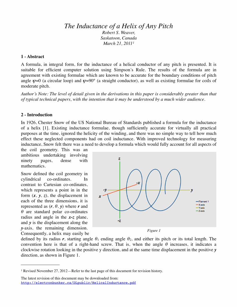
2 - IntroductionIn 1926, Chester Snow of the US National Bureau of Standards published a formula for the inductance of a helix [1]. Existing inductance formulae, though sufficiently accurate for virtually all practical purposes at the time, ignored the helicity of the winding, and there was no simple way to tell how much effect these neglected components had on coil inductance. With improved technology for measuring inductance, Snow felt there was a need to develop a formula which would fully account for all aspects of the coil geometry. This was an ambitious undertaking involving ninety pages, dense with mathematics. Snow defined the coil geometry in cylindrical co-ordinates. In contrast to Cartesian co-ordinates, which represents a point in in the form (x, y, z), the displacement in each of the three dimensions, it is represented as (r, θ, y) where r and θ are standard polar co-ordinates radius and angle in the x-z plane, and y is the displacement along the y-axis, the remaining dimension. Consequently, a helix may easily be defined by its radius r, starting angle θ1 ending angle θ2, and either its pitch or its total length. The convention here is that of a right-hand screw. That is, when the angle θ increases, it indicates a clockwise rotation looking in the positive y direction, and at the same time displacement in the positive y direction, as shown in Figure 1.

1 Revised November 27, 2012—Refer to the last page of this document for revision history.

The latest revision of this document may be downloaded from:http://electronbunker.ca/DLpublic/HelicalInductance.pdf

Figure 1

http://electronbunker.ca/DLpublic/HelicalInductance.pdf

http://electronbunker.ca/DLpublic/HelicalInductance.pdf

This helix is defined by three parametric equations:x=r cos θ (1A)y=p θ (1B)z=−r sin θ (1C)where r is the radius of the helix, and 2πp is the pitch. It should be noted that Snow has used a rather unconventional definition for pitch. Pitch normally refers to the centre to centre spacing of the helix measured parallel to the axis of the coil. However this value differs from p by a factor of 2π. This is merely a convenience to simply the mathematics, and the factor of 2π may be re-introduced later to restore the normal meaning. For the purpose of this discussion, the variable p will be referred to as the pitch factor to distinguish it from pitch.The foundation of Snow’s work was the development of a formula for the mutual inductance of two helical filaments (as illustrated in Figure 2), of N turns, radii r1, r2, axial offset y1, y2: and pitch 2πp. It was in the form of a double integral for which he developed a closed form solution using certain approximations. This was then integrated over the cross-section of the conductor to get the self inductance. It is important to note that Snow’s chosen geometry has the conductor’s starting cross section parallel to the x-y plane, rather than normal to the direction of the helix. For helices of small pitch, these are approximately the same. However, this will introduce distortion which makes it unsuitable for helices of larger pitch. Snow’s helical mutual inductance formula is as follows:

(2)Where:

R2 = r21 + r2

2 ! 2r1r2 cos(!2 ! !1) .

Upon review of Snow’s work, it became apparent that the term to the left of the integral has been simplified in a way which has no significant effect on helices of small pitch (which were of primary interest to Snow), but again, creates problems for large pitch helices.

The Inductance of a Helix of Any Pitch

— 2 —

Figure 2

The corrected formula should be:

(3)Snow then reduced the mutual inductance formula (2) to a single integral. It was my original intention to solve the single integral, using Simpson’s Rule and the method of geometric mean distances, to create a computer program function to solve for self inductance. While this did give good results, it was only accurate when pitch was small. It is quite apparent that Snow’s formula, as it stands, is not suitable for coils of large pitch.A review of the technical literature shows that, in the decades following Snow's work, except for finite element methods, little has been done on the subject of inductance calculation where helicity is taken into account. However, this has changed in recent years; research in flux compression generators has resulted in renewed interest in inductance calculations where helicity is addressed [3][4]. Upon review of the recent literature however, it appears that a geometrically derived helical inductance formula is still of value, and may yet lead to the most efficient method of calculation. For example, the method of reference [4] only claims an accuracy of 5%. The present work results in a calculation method which is in exact agreement2 with well established formula, in all comparable cases, and is expected to be equally accurate in the intermediate cases. To adapt Snow's work so that it is suitable for helices of any pitch, it is necessary to re-derive the mutual inductance formula in such a way that the inappropriate approximations are removed, and that the singularities which appear in Snow's formula, when pitch is infinite, do not occur. In doing this, there are three issues which need to be addressed. These are discussed in the next section, and the new formula derivation is given in the subsequent sections.

3 - The Pitfalls of Coils and Three-Dimensional GeometryThe problems needing to be addressed in the present work are:• The distortion of the conductor cross-section (in the plane parallel to the coil axis) when pitch is

large;• The case when pitch approaches–and becomes–infinity;• The case when the limits of integration narrow to zero.All of these are different aspects of the same condition, that is, when the pitch is very large, and when it approaches infinity.The first item has already been discussed briefly. The problem exists because the original formula requires that the endpoints of both helices be at θ=0. This is corrected by allowing the second filament to start at an initial angle of θ0, as well as an offset along the y-axis; it is possible to arrange the two filaments such that they both have their starting points in a plane that is normal to them both, and where their distance of separation is a specified value.The second item requires that the pitch factor p cannot appear in the formula. Instead, the pitch angle ψ, and finite functions thereof, will be used.


— 3 —2 Exact within the limitations of double precision computer mathematics, i.e., 15 significant digits.

The third item requires that the main parametric variable and variable of integration, θ, must be replaced with another variable which does not tend towards a constant when pitch approaches infinity. The variable to be used is defined as s, the distance along the filament measured from its starting point.There are a few other miscellaneous pitfalls which crop up when dealing with coil geometry, which will now be addressed.Figure 3 represents what would happen if we cut open one side of a three turn coil along its length parallel to its axis and then spread it out flat, while keeping the conductors in their respective positions.Alternatively, we can think of it as wrapping a cylindrical coil form with paper, then drawing a picture of the conductors on it, then removing the paper and laying it flat. In any event, it shows that when pressed flat, the formerly helical conductors are now straight lines, and we can apply two dimensional geometry (with a few restrictions) in order to take measurements.The coil radius, D/2, is taken to the centre of the conductor, so that in the figure, the conductors extend past the coil form outline by half of a conductor diameter on both top and bottom. Conductor diameter will be represented here by the variable dW.The pitch in the diagram is large in order to highlight the fact that the pitch 2πp is greater than the centre to centre spacing p′. It is also apparent that the cross section of the conductor, taken at the angle shown here, will be very slightly elliptical. It becomes extremely elliptical as the pitch becomes much larger. As a corollary, the pitch of a close-wound coil must always be greater than the conductor diameter. In fact the minimum possible pitch angle ψc is:ψc = Arcsin(dW/(πD)) (4)where dW is wire diameter and D is coil diameter.This concept, where the surface of the cylinder is unwrapped and laid flat, gives a handy tool which will come up again. In engineering drafting terminology, this is actually called a developed view or simply a development. It is useful to note that all lines, curved or straight, appearing on such a diagram, as long as they had lain on the surface of the cylinder, are shown as their true length.


— 4 —

Figure 3

4 - Useful Trigonometric PrinciplesBefore getting into the actual derivation of the inductance formula, a few small but important items are presented here. The following trigonometric formulae will be used several times in the course of the derivation, so they are given here for future reference. The equation numbers are those of Dwight [5] from where these were taken:sin2 A + cos2 A = 1 (400.01)2 cos A cos B = cos (A+B) + cos(A−B) (401.06)2 sin A sin B = cos (A−B) − cos(A+B) (401.07)The first is well known, and a direct application of the theorem of Pythagoras. The other two are less obvious but equally important.We now move on to the measurement of circular arcs and other related geometry, referring to Figure 4. In keeping with prior convention, the working plane for the polar components is the x-z plane. We are looking in the positive y direction (the negative y axis is coming out of the page towards us).The blue line s is an arc of radius r, starting at point a and ending at point b. As mentioned previously, by our convention, angles are measured from the positive x-axis, and clockwise angles (when looking in the positive y direction) are positive, and counter-clockwise angles are negative. Therefore, θ1 is negative, and θ2 is positive. The total angle subtended by arc s is θ which is equal to θ2−θ1.Because we are measuring angles in radians, the length of s is simply rθ or r(θ2−θ1). Generally, the length of any arc will be r(θ2−θ1) where θ1 and θ2 are the start and end angles of the line, and r is the radius. Note however, that the distance between points a and b is not equal to the length of s. It is equal to the length of the straight (red) line joining a and b. However, except in one situation which will be discussed later, we are not interested in the straight line distance; we are generally only concerned with the distances measured along the arc.Now, returning to the developed view, we see in Figure 5 a different line s1 which is a helical arc with pitch denoted by the angle ψ. It was previously stated that all lines, curved or straight, appearing on such a diagram, as long as they had lain on the surface of the cylinder, are shown as their true length. In the case of straight lines which are horizontal in this view, then the length is simply |y1−y0|, where y1 and y0 are the y co-ordinates of the endpoints. Lines which appear vertical in this view may be measured using the methods shown for Figure 4.


— 5 —

Figure 4

In this case however, line s1 is neither vertical nor horizontal. From the Pythagorean theorem the length of s1 is given by:s1 = √(r2 θ2 + y12)This also provides a means to relate the the variable θ of the parametric equations (1A, 1B, 1C) of the helix to the variable s, the distance along the filament. From trigonometry:rθ = s1 cos ψOr:θ = s1 (cos ψ)/rIt will prove convenient (and save much writing) to define this constant:kψ = (cos ψ)/r (5)

Now referring back to the helical filament (blue line in Fig. 5), we can relate the angle θ to the distance s along the filament.In the case of filament 1:θ1 = (s1/r)cos ψ = kψ s1 (6A)It can also be seen from Figure 5, that there is a direct trigonometric relationship between y1 and s1:y1= s1 sin ψ (6B)and in the case of filament 2, because it has a non-zero starting angle and a y offset:θ2 = (s2/r)cos ψ + θ0 = kψ s2 + θ0 (6C)y2= y0 + s2 sin ψ (6D)

5 - The Mutual Inductance of Two Helical FilamentsThe Neumann Integral will be the means used here to calculate the mutual inductance of two helical filaments. Discussion of the underlying physics will not be attempted. The reader should refer to one of the many resources on the subject of electricity and magnetism. The Neumann Integral is:

(7)The integral is taken over the lengths of the two filaments. Like many formulae from physics, it appears beautifully simple until you try to apply it. For example, the innocuous little dot between ds1 and ds2, is there to warn the reader that there's a lot of 3D trigonometry coming up. Or, in more precise terms, it's a dot product, meaning that we are doing a scalar multiplication of two vectors, in this case: ds1 and ds2. It


— 6 —

Figure 5

means that we multiply the x components of each vector, then the y components, then the z components, and finally add these three separate results together to get a non-vector (scalar) number. Alternatively—the approach to be used here—we can simply multiply the magnitudes of the vectors and then multiply the result by the cosine of the angle of inclination, of the two vectors. The cosine of the angle of inclination, cos ϵ, can be calculated by taking the dot product of the direction cosines of ds1 and ds2. The direction cosines are:

dxds , dy

ds , dzds .

So, to get the direction cosines, we need to find formulae for x, y and z in terms of s, and then take the derivatives. To find these, we combine formulae (1A) and (1C) which give x, and z in terms of θ, with formulae (6A..D), giving for filament 1:x1 = r cos (kψs1) (8A)y1 = s1 sin ψ (8B)z1 = −r sin ( kψs1) (8C)and for filament 2:x2 = r cos ( kψs2 + θ0) (8D)y2 = s2 sin ψ + y0 (8E)z2 = −r sin ( kψs2 + θ0) (8F)Now taking the derivatives with respect to s, gives for filament 1:dx1/ds1 = −cos ψ sin (kψs1) (9A)dy1/ds1 = sin ψ (9B)dz1/ds1 = −cos ψ cos (kψs1) (9C)And for filament 2:dx2/ds2 = −cos ψ sin (kψs2 + θ0) (9D)dy2/ds2 = sin ψ (9E)dz2/ds2 = −cos ψ cos (kψs2 + θ0) (9F)These are our direction cosines.

Finally multiplying the corresponding direction cosines to get cos ϵ:

cos ϵ = (−cos ψ sin (kψs1))(−cos ψ sin (kψs2 + θ0))+(sin ψ)(sin ψ) + (−cos ψ cos (kψs1))(−cos ψ cos (kψs2 + θ0))Collecting terms:

cos ϵ = cos2 ψ[(sin (kψs1) sin (kψs2 + θ0))+(cos (kψs1) cos (kψs2 + θ0))] + sin2 ψNow we apply Dwight’s (401.06) and (401.07) to change the products of the sines and cosines to sums:

cos ϵ = ½cos2 ψ[cos (kψs1 − kψs2 − θ0) − cos (kψs1 + kψs2 + θ0) + cos (kψs1 + kψs2 + θ0) + cos (kψs1 − kψs2 − θ0)] + sin2 ψCombining equal terms:

cos ϵ = cos2 ψ cos (kψ(s1 − s2) − θ0) + sin2 ψ (10)which gives the numerator of the Neumann Integral.


— 7 —

The variable R in the denominator of the Neumann Integral is the Euclidian distance between the two infinitesimal line segments ds1 and ds2. In Cartesian coordinates:R2 = (x1−x2)2 + (y1−y2)2 + (z1−z2)2 (11)where subscripts 1 and 2 correspond to filaments 1 and 2 respectively. Substituting (8A..F) into (11) gives:R2 = r2[(cos(kψs1) − cos(kψs2 + θ0))2 + (sin(kψs1) − sin(kψs2 + θ0))2] + ((s1−s2)sin ψ − y0)2

Expanding the squared terms:R2 = r2[cos2(kψs1) + cos2(kψs2 + θ0) − 2 cos(kψs1) cos(kψs2 + θ0) + sin2(kψs1) + sin2(kψs2 + θ0) − 2 sin(kψs1) sin(kψs2 + θ0)] + ((s1−s2)sin ψ − y0)2

Applying Dwight’s (400.01) will simplify the sin2 and cos2 terms: R2 = r2[2 − 2 cos(kψs1) cos(kψs2 + θ0) − 2 sin(kψs1) sin(kψs2 + θ0)] + ((s1−s2)sin ψ − y0)2

Applying Dwight’s (401.06) and (401.07) will convert the products of sines and cosines to sums:R2 = r2[2 − cos(kψs1 + kψs2 + θ0) − cos(kψs1 − kψs2 − θ0) − cos(kψs1 − kψs2 − θ0) + cos(kψs1 + kψs2 + θ0)] + ((s1−s2)sin ψ − y0)2

Combining terms:R2 = r2[2 − 2 cos(kψs1 − kψs2 − θ0)] + ((s1−s2)sin ψ − y0)2

Taking the square root of both sides:

R =!

r2[2! 2cos(k!(s1 ! s2)! !0] + [(s1 ! s2)sin" ! y0]2 .

(12)which gives the denominator of the Neumann Integral.As was mentioned earlier, the limits of integration will be across the length of the filaments, or from 0 to ℓW, where ℓW is the total length of the filament. Combining (7), (10) and (12), we get:

(13)Following the method used by Snow [1], we now we define a new variable φ as:

! = s1 ! s2 . (14)

which allows us to replace the two variables in the integrand, s1 and s2, with just φ. We also replace ds1 using the following identity:

d!ds1

= dds1

(s1 ! s2) = 1 .

(15)Hence:

d! = ds1 . (16)


— 8 —

We must also change the limits of the ∫ dφ integral, using the substitution (14), so that the lower limit is:φ= 0 − s2 = −s2

and the upper limit is:

φ= ℓW − s2

Hence:

(17)For any given helix, φ is the only variable in the integrand. For this reason, and also because the integrand will not be simplified any further, the integrand will henceforth be represented by f(φ):

f(!) =cos2 " cos(k!!! #0) + sin2 "!

r2[2! 2 cos(k!!! #0)] + [! sin " ! y0]2.

(18)This simplifies the writing of the mutual inductance formula (17) to:

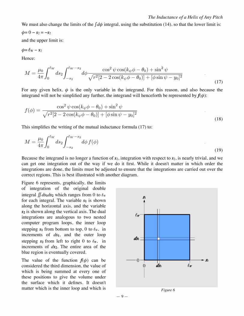
(19)Because the integrand is no longer a function of s2, integration with respect to s2, is nearly trivial, and we can get one integration out of the way if we do it first. While it doesn't matter in which order the integrations are done, the limits must be adjusted to ensure that the integrations are carried out over the correct regions. This is best illustrated with another diagram. Figure 6 represents, graphically, the limits of integration of the original double integral ∫∫ ds1ds2 which ranges from 0 to ℓW for each integral. The variable s1 is shown along the horizontal axis, and the variable s2 is shown along the vertical axis. The dual integrations are analogous to two nested computer program loops, the inner loop stepping s1 from bottom to top, 0 to ℓW, in increments of ds1, and the outer loop stepping s2 from left to right 0 to ℓW, in increments of ds2. The entire area of the blue region is eventually covered. The value of the function f(φ) can be considered the third dimension, the value of which is being summed at every one of these positions to give the volume under the surface which it defines. It doesn't matter which is the inner loop and which is


— 9 —Figure 6

the outer loop. The result is the same.Now, in the case of the double integral ∫∫ ds2dφ, the region of integration is as shown in Figure 7. The limits are skewed because the ∫ dφ integral's limits are functions of s2. If the outer integral is ∫ ds2 and the inner integral is ∫ dφ, then the evaluation still proceeds the same as before: the inner integral variable φ stepping from bottom to top ranging from −s2 to ℓW−s2, while the outer integral variable s2 steps from 0 to ℓW.However, if the order of integration is reversed, then the limits of the ∫ ds2 integral will change as φ passes through zero. That is, the limits in the upper (red) region are different from the limits in the lower (blue) region. In order to handle this, we simply break up the original integrals into two separate parts. The first will evaluate the limits of the lower region, with the limits of ∫ ds2 ranging from −φ to ℓW, while ∫ dφ limits are from −ℓW to 0. The second will evaluate the upper region with ∫ ds2 limits from 0 to ℓW−φ, while ∫ dφ limits are from 0 to ℓW.Hence, we now have:

(20)Now, integrating both parts with respect to s2 gives:

(21)Because it is very difficult, if not impossible, to evaluate these remaining integrals analytically, they will be left as is, and solved numerically, using Simpson's Rule.

6 - The Self Inductance of a Helical ConductorMaxwell [6a][7], showed that if a formula exists for the mutual inductance between two identical parallel filaments, then it may be used to calculate the self inductance of a finite conductor of the same geometry by applying the principle of geometric mean distances. Simply stated, if we set the distance separating the two filaments equal to the GMD (geometric mean distance) of the finite conductor’s cross


— 10 —

Figure 7

section, then the value obtained from the mutual inductance formula (in this case, formula (21)) will be equal to the self inductance of the conductor. This is generally valid as long as the conductor diameter is much smaller than the coil diameter. Grover [8], chapter 3, gives formulae for the geometric mean distances for several different shapes. The one most commonly required, corresponding to solid round wire, is the GMD of a circular area which is given as:

g = re−¼ = 0.7788rwhere g denotes the GMD, r is the radius of the conductor, and e is the base of natural logarithms. Knowing that the distance separating the two filaments is g, we must now convert that into the appropriate values for θ0 and y0. It's time for another diagram.Figure 8 is another developed view of the coil form cylinder which shows the start points p1 and p2 of filaments F1 and F2 respectively. In order to maintain a reasonable spatial relationship, the line g′ joining points p1 and p2 should be perpendicular to both F1 and F2 for any pitch angle. This ensures that the distance between corresponding points on the respective filaments will always be the same, and this can be made equal to the value of g.The line h′ has a length equal to rθ0. The line g′ has a length approximately, but not exactly, equal to g. We want the distance between p1 and p2 to be exactly equal to g. However, due to the curvature of the surface of the cylinder, the distance between them is slightly less than the length of g′. This is explained by referring back to Figure 4, which shows the end view of the cylinder; the straight (red) line between points a and b gives the distance between a and b which is less than the length of the arc s. The situation is the same here, with the single exception that when ψ=0, then g=g′. In all other cases: g<g′. Recalling that we can calculate the distance between two points using (11), replacing R with g gives:g2 = (x1−x2)2 + (y1−y2)2 + (z1−z2)2 (22)In this instance, y0=y2−y1, x1 =r, and z1 =0. Hence:g2 = (r−x2)2 + y02 + z22 (23)Then substituting in the polar parametric equations (1A), (1B), (1C):g2 = r2 cos2 θ0 + p02 θ02 + r2 sin2 θ0 + r2 − 2r2 cos θ0

Using Dwight’s (400.01) the sin2 and cos2 terms can be removed:g2 = 2r2 (1−cos θ0) + p02 θ02 (24)


— 11 —

Figure 8

In this case the pitch factor p0 refers to the pitch of the line g′, not the pitch of the filaments. The pitch angle of g′ will be designated ψ0 and is given as:ψ0 = π/2 − ψ (25)where angles are in radians. And then p0 is given by:p0 = r tan ψ0 (26)Substituting (26) into (24) and moving all terms to the same side of the equals sign gives:g2 − 2r2 (1−cos2 θ0) + r2 θ02 tan2 ψ0 = 0 (27)The only unknown in this equation is θ0. Unfortunately, there is no closed form solution for θ0. However, it can be solved very efficiently using the Newton-Raphson method, starting with an approximate value for θ0 of:θ0 = g/r sin ψ (28)The solution converges within the limits of double precision arithmetic in only a couple of iterations. (In fact, the approximate starting value given by formula (28), is probably close enough to the exact value, for all practical purposes.) Once θ0 has been calculated, the the calculation of y0 follows directly from (24):y0 = √(g2 − 2r2(1−cos θ0)) (29)There are two special cases where θ0 can calculated directly. In the case ψ=0, then θ0 =0 and y0=g. In the case ψ=90° = π/2 radians, then y0=0 and:θ0 =Arccos(1−g2/(2r2)) (30)It should be noted, using the convention adopted in this work, that y0 is always greater than or equal to zero, and θ0 is always less than or equal to zero.This completes the calculation of all of the input arguments to the helical inductance formula. In the next section, details are given of the implementation of the numerical integration using Simpson's Rule.

7 - Simpson's RuleSimpson's Rule is a well known numerical method for evaluating integrals. To evaluate the integral of a function f(x) over the range x=[a..b], the function to be integrated is evaluated at three points a, b and m, where m is the midpoint between a and b.m=(a+b)/2The area under a parabolic curve which passes through the three points f(a), f(b) and f(m) is used as an approximation of the true value of the integral.The approximate value of the integral, using the parabolic curve, is then given by:

(31)It should be obvious that the accuracy of this approximation will depend on how well a parabola fits the actual function. In practice, the interval over which we wish to integrate will be broken into smaller sub-intervals, with Simpson's Rule applied to each sub-interval. This is known as Composite Simpson’s Rule.


— 12 —

If we break the interval into n subintervals, then Composite Simpson's Rule gives:

(32)A few things to note:• There is always an even number of intervals, which means that there will be an odd number of points

evaluated;• The odd numbered points have a coefficient of 4;• The even numbered points (except x0 and xn) have a coefficient of 2;• The end points x0 and xn have a coefficient of 1;• The more points evaluated, the more accurate the result.It's apparent that we can evaluate the function for all of the values of x using a program loop, and apply the correct coefficient depending on whether the subscript of the x value is even or odd. However, a more efficient method is to maintain two summations, one for the even values and one for the odd values, and then multiply these sums by the appropriate coefficient. A less obvious reason for doing this is that if using n sub-intervals doesn't give us the desired accuracy, we can double the number of sub-intervals, and the points that had been previously calculated can be reused. All of the previous odd and even points will become the new even numbered points, and only the new odd numbered points (which will fall between the old points) will be evaluated.The program was set up so that the integration would start with a single interval, and then split it in half, doubling the intervals each time through the main program loop, until acceptable precision is reached.In testing the routine, it was found that in order to achieve acceptable accuracy, the number of integration sub-intervals was excessive. This can be explained by looking at a graph of the Integrand function f(φ). Figure 9 shows the function for a typical coil with φ on the horizontal axis. When φ ≈ 0, this corresponds to the situation where the two filamental elements are in closest proximity, and the function has a very sharp peak. In this region, the intervals need to be very small. As φ increases, the intervals can increase in size. To achieve this, an additional outer program loop was added to break up the integration into unequal segments. The first in the region of φ ≈ 0 being the smallest, and then each successive segment doubling in size. This works very well, markedly reducing the number of function evaluations. The program was coded in Open Office Basic, because it is widely accessible, and the program may be implemented as a spreadsheet function allowing for convenient inductance calculation on the spreadsheet. The program code listing is in Appendix A. For the following detailed discussion, please refer to that listing.


— 13 —

Figure 9 φ→

f (φ

)→

The main function is called HeliCoilS(). The code for f(φ), formula (18), is evaluated by a separate function Ingrnd(), because it needs to be evaluated in several different places in the main function. The function header for Ingrnd() is:Function Ingrnd (byval phi as double, kphitheta as double, sinpsi as double,

cos2psi as double, rr as double, y as double) as double

To speed execution, the values kψφ−θ0, cos2 ψ, sin ψ and r2 are pre-calculated in the main function.When executing HeliCoilS(), the calling parameters are:Function HeliCoilS (byVal Lw as double, psi as double, r as double,

dw as double, MaxErr as double) as double

Where:Lw = ℓW the total length of conductor in the coil (meters)psi = ψ the pitch angle (radians)r = r the coil radius (meters)dw = dW the conductor diameter (meters)MaxErr = required precision of the resultThe value returned by HeliCoilS() is inductance in Henries.The parameter MaxErr requires a bit of explanation. The inner While loop terminates when the difference in the integral values between successive iterations vary by less than MaxErr. The outer While loop then increments to the next interval to be evaluated. When all intervals have been evaluated, the function terminates. Because of the way that MaxErr is used, there is no direct relationship between it and the precision of the final result. This unfortunately, is a limitation in numerical integration methods. In practice, it is recommended to start with a modest value for MaxErr, such as 0.01, and then make it smaller until no difference is found in the results. Given the prior knowledge that f(φ) has a sharp spike near φ=0, the use of intervals of increasing size, in the outer loop, works well to minimize inaccuracy. On the subject of interval sizes, the hard-coded value of 32768 is used in the program line:b=Lw/32768

to set the first interval to 1/32768th of the total conductor length. Each successive interval is double the size of the previous one. However, each of these intervals will be split in half and evaluated at least once in the inner loop, to ensure that the MaxErr condition is satisfied. The value 1/32768 was set arbitrarily small and some further experimentation may be in order to find the optimum value. However the optimum is likely to vary depending on the coil geometry. Likewise, the hard-coded minimum iteration count of 512 in the inner While loop may be subject to some further optimization.In normal practice, coil parameters are likely to be given as total number of turns N and either pitch or total coil length, ℓCOIL, rather than ψ and ℓW. However, these may be converted as follows:

pitch = 2πp = ℓCOIL/N ψ = Arctan(pitch/(πD)ℓW = N√(pitch2+(πD)2)where pitch is the centre to centre spacing of the turns measured parallel to the y-axis; i.e., it is the standard definition of pitch.


— 14 —

8 - ResultsThe point of all this was to arrive at a function that is accurate for any pitch. It is instructive therefore, to see what happens when we take a fixed length of wire, and a coil-form of a given diameter, so that a coil may be wound of any pitch (varying from 0 to ∞ as ψ varies from 0 to 90°), and we can see how the inductance varies with pitch. (It is, of course, somewhat unconventional to use a fixed conductor length rather than, say, a fixed number of turns. However, a fixed number of turns is not possible when pitch becomes infinite.) As an example, a conductor of length 5000 mm, and diameter of 1 mm will be used, with coil diameter fixed at 25 mm. As pitch increases, the number of turns decreases and the coil length increases. Conversely, as pitch decreases, the number of turns increases and coil length decreases.Figure 10 shows the results:

Figure 10

The violet line indicates how the number of turns of the coil decreases as ψ increases, reaching exactly zero, as it should, when ψ=90°.The blue line is the inductance calculated by the new formula. As the pitch angle increases, the inductance drops off and then rises again, reaching the straight conductor inductance value (red dashed line), as it should, when ψ=90°.


— 15 —

The fact that the minimum value of inductance is less than that of a straight conductor is not surprising, because the current flowing in diametrically opposed elements will cause cancellation, and when the pitch increases to a certain point, adjacent conductors are no longer close enough to each other to have a multiplicative aiding effect. It should also be noted that we are dealing with partial inductance here, not loop inductance (except in the singular case when ψ=0). In order to close the loop, other factors come into play which will affect the inductance of the complete circuit.As previously noted, the red dashed line indicates the inductance of a straight conductor. It has been calculated, for comparison purposes, from a formula given by Grover. An approximate formula for the inductance of a straight conductor (Grover [8], page 35) is:

L = 0.002!W

!ln

"4!W

dW

#! 3

4

$

(33)However, using the exact straight filament mutual inductance formula (Grover [8], page 31), a slightly more accurate straight conductor self inductance formula can be derived:

L = 0.002!W

!

"ln

#

$ !W

kgdw+

%

1 +&

!W

kgdw

'2(

)!

%

1 +&

kgdw

!W

'2

+kgdw

!W

*

+

(34)In both (34) and (35) dimensions are in cm, inductance is in µH, and the constant kg is given by:

kg =e!

14

2= 0.3894

Because the goal is to compare the present work with the most accurate formulae available, formula (34) will be used here, although (33) and (34) generally agree to six significant figures.The original Snow formula (green curve), and Rosa's formula3 (red curve, see Grover [8], page 149) are provided for comparison. Rosa's formula is included, because it is arguably the most accurate of the well known current sheet based inductance formulae. Here, Rosa's formula begins to deviate from the helical formulae as ψ exceeds 5°. Snow's original formula4 starts to deviate from the new formula at about ψ=15°.


— 16 —

3 Rosa's formula is based on the Lorenz current sheet formula (or Nagaoka's variation of it), but includes round wire corrections which are tabulated in Grover's book to four decimal places. However, the round wire corrections were recalculated to ten decimal places in 2008. See ref. [9]. These more precise values are used in the comparisons presented here.

4 For practical reasons, Snow's original formula is not implemented here exactly as he developed it. Snow developed a rather involved closed form formula based on his helical filament mutual inductance integral formula. However, it included some functions, the values of which, had to be read from graphs. The calculation used here is a Simpson's Rule implementation of his mutual inductance integral, as it is more suitable for computer calculation. The implementation used here was verified using examples which Snow provided in his paper [1].

Figure 11 shows the same comparison expanded to show only the range ψ=0 to 12°:

Figure 11

In this range, the curves for Snow's original formula and the present helical formula are indistinguishable, while the curve for Rosa's formula is very close.As the above curves are too cramped to read numerical values accurately, the actual program output values are provided in the following table, for comparison:


— 17 —

Coil 1 – As shown in preceding graphs;ℓW = 5000 mm; dw = 1 mm; D = 25 mm

Coil 2 – Exactly one single turn when ψ =0;ℓW = 3141.59 mm; dw = 1 mm; D = 1000 mm

ψ = ψC = 0.72953° (Close-wound coil):LHEL = 32.8527 µH (New helical formula)LSNOW = 32.8474 µH (Snow's original formula)LROSA = 32.5840 µH (Rosa's formula)

ψ = 0 (Circular Loop):LHEL = 4.5473 µHLSNOW = 4.5473 µHLROSA = 4.5473 µH (coil length set equal to dw)LMAXWELL = 4.5473 µH

(Maxwell's [6b] loop inductance formula)

ψ = 5°:LHEL = 6.8808 µHLSNOW = 6.8304 µHLROSA = 6.6018 µH

ψ = 30°:LHEL = 4.8484 µHLSNOW = 3.6690LROSA = 4.1610

ψ = 15°:LHEL = 5.0111 µHLSNOW = 4.6914 µHLROSA = 3.8823 µH

ψ = 45°:LHEL = 5.1458 µHLSNOW = 2.6226LROSA = 3.5433

ψ = 90° (Straight Conductor):LHEL = 9.1536 µHLLINEAR = 9.1536 µH

(Straight conductor formula, Grover [8] pg. 35)LSNOW = N/ALROSA = N/A

ψ = 90° (Straight Conductor):LHEL = 5.4594 µHLLINEAR = 5.4594 µHLSNOW = N/ALROSA = N/A

As can be seen, the new formula shows good agreement with the Snow and Rosa formulae when ψ is small, and good agreement with the straight conductor formula when ψ is 90°.In the second example, Coil 2 is a single circular loop when the pitch angle ψ=0. Although the values for Snow's and Rosa's formulae have been included for ψ=30° and ψ=45°, it is just for interest sake; they are not expected to produce useful values at these pitch angles. Figure 12 shows the variation of inductance with pitch for Coil 2. Again the dashed red line indicates the inductance of the straight conductor. Because the conductor becomes a circular loop when ψ=0, this provides yet another point of comparison. Maxwell's elliptic integral formula for the inductance of a


— 18 —

Figure 12

circular loop [6b] is used to provide comparative values in this case, and the agreement is essentially exact.It is appropriate at this point, to comment on the performance of the computer program. It was stated above that it was coded in Open Office BASIC due to its wide availability. It is certainly not a fast implementation of BASIC, and is rather outdated even compared to other BASIC implementations. However, even with these limitations, the subroutine was able to calculate the inductance of almost any practical coil in a fraction of a second on a Macintosh MacBook Pro with 2.4 GHz Intel Core 2 Duo processor. This can be considered fairly typical personal computer hardware at the time of this writing. For practical applications, more efficient programming languages should provide considerable performance improvement. This would appear to be compare well with other current computer methods [3][4].Performance does decrease noticeably, for coils where the conductor diameter is extremely small compared to coil diameter, and with a very large number of turns. This occurs because, in this case, the integrand function exhibits numerous periodic spikes, which taxes the numerical integration method. However, in these special cases, this formula would offer little to no improvement in accuracy over existing inductance calculation methods. On the other hand, coils having large pitch will generally have relatively few turns, and in these cases, the method presented in this paper is quite efficient.

9 - ConclusionThe formula presented here has been shown to agree with other existing formulae in those cases where such formulae are applicable and known to be accurate, i.e., small pitch, and infinite pitch. I am not aware of any formula which may be used as a cross-check for the intermediate pitch angles (ψ=45°, for example), and I have not yet attempted to verify the formula by experiment. Therefore, further work is required (possibly finite element methods) to verify the midrange-ψ inductance values. Because the Simpson's Rule implementation requires considerably more computation than traditional inductance formulae, it is not expected that this new calculation method will replace existing ones, except in those cases where coil pitch is significant. However, this new calculation method may be used as an aid in developing a simpler empirical formula. Work in this area is currently underway.Rosa's formula continues to stand the test of time. It is in good agreement for ψ≤5°, and it should be pointed out that ψ=5° amounts to quite significant pitch (0.275 times the coil diameter), not likely to be encountered in coils used below VHF/UHF frequencies.


— 19 —

10 - References1. Snow, Chester; Formula for the Inductance of a Helix Made With Wire of Any Section, US National

Bureau of Standards Scientific Paper No. 537. Vol. 10, November 1926.2. Snow, Chester; A Simplified Precision Formula for the Inductance of a Helix with Corrections for

the Lead-In Wires, NBS Journal of Research Vol. 9, RP479, June 1932.3. Schnurr, N.M.; Report LA-10056-MS, Los Alamos National Lab., May 1984.4. Sijoy C.D. and Chaturvedi, S.; Fast and Accurate Inductance Calculations for Arbitrarily-Wound

Coils for Pulsed Power Applications, IEEE Pulsed Power Conference, 20055. Dwight, Herbert B.; Tables of Integrals and other Mathematical Data; Fourth Edition, MacMillan,

1961.6. Maxwell, James Clerk; A Treatise on Electricity and Magnetism, Vol. 2, Third Edition, Dover 1954;

(a) Art. 691, On the Geometrical Mean Distance of Two Figures on a Plane, pp. 324-326.(b) Art. 701, To find M by Elliptic Integrals, pp. 338-340.

7. Maxwell, James Clerk; On the Geometrical Mean Distance of Two Figures on a Plane, Transactions, Royal Society of Edinburgh, Vol. XXVI.

8. Grover, Frederick W.; Inductance Calculations–Working Formulas and Tables, D. Van Nostrand, 1946; Reprint: Dover, 2004.

9. Weaver, Robert; Investigation of E.B. Rosa's Round Wire Mutual Inductance Correction Formula, July 2008.


— 20 —

http://electronbunker.ca/DL/Sci537_Snow_Helix.pdf

http://electronbunker.ca/DL/Sci537_Snow_Helix.pdf

http://electronbunker.ca/DL/Snow_RP479.pdf




http://electronbunker.ca/DLpublic/Rosa_Derivation.pdf

http://electronbunker.ca/DLpublic/Rosa_Derivation.pdf

Appendix AHelical Inductance Program Code - Open Office BASIC:Function HeliCoilS (byVal Lw as double, psi as double, r as double, dw as double, MaxErr as double) as double' Uses helical filament mutual inductance formula evaluated using' Simpson's rule, and conductor gmd' Lw = total length of wire' psi = pitch angle of winding' r = radius of winding' dw = wire diameter' MaxErr = max allowable error'' If Lw>2*pi*r, check that pitch angle >= psi-c (close wound pitch) If Lw>2*pi()*r then sinpsic=dw/(2*pi()*r) psic=atn(sinpsic/sqr(1-sinpsic*sinpsic) if psi<psic then' pitch angle is too small,' so set value of function to an illegal value and exit HeliCoilS=1e200 Exit Function end if End if' gmd of solid round conductor. Other values may be substituted' for different conductor geometries g=exp(-.25)*dw/2 rr=r*r psio=0.5*pi()-psi' Calculate Filament 2 offset angle' Trap for psi=0 condition in which case ThetaO=0 and Y0=g' Trap for psio=0 condition in which case use simplified' formula for ThetaO and Y0=0' which happens with circular (non-helical) filament if psi=0 then ThetaO=0 Y0=g ElseIf psio=0 then cosThetaO=1-(g*g/(2*rr)) ThetaO=-abs(atn(sqr(1-cosThetaO*cosThetaO)/cosThetaO) Y0=0 Else' Use Newton-Raphson method k1=(g*g)/(2*r*r)-1 k2=tan(psio) k2=0.5*k2*k2 t1=g/r*sin(psi) do t0=t1 t1=t0-(k1+cos(t0)-k2*t0*t0)/(-sin(t0)-2*k2*t0) Loop until abs(t1-t0)<1e-12 ThetaO=-abs(t1)' Calculate Filament 2 Y-offset, using formula (29) Y0=sqr(g*g-2*rr*(1-cos(ThetaO))) End if


— A-1 —

' Psi constants c2s=cos(psi)^2 ss=sin(psi) k=cos(psi)/r' Start of Simpson's Rule code a=0 b=Lw/32768 If b>Lw then b=Lw grandtotal=0 Do while a<Lw dx=b-a m=1 CurrentErr=2*MaxErr kat=k*a kbt=k*b Sum2=(Lw-a)*(Ingrnd(-a,-kat-ThetaO,ss,c2s,rr,Y0)+Ingrnd(a,kat-ThetaO,ss,c2s,rr,Y0)) + (Lw-b)*(Ingrnd(-b,-kbt-ThetaO,ss,c2s,rr,Y0)+Ingrnd(b,kbt-ThetaO,ss,c2s,rr,Y0))' Initialize LastResult to trapezoidal area for termination test purposes LastIntg=Sum2/2*dx Do While CurrentErr>MaxErr or m<512 m=2*m dx=dx/2 Sum=0 SumA=0 for i=1 to m step 2 phi=i*dx+a kpt=k*phi Sum=Sum+ (Lw-phi)*(Ingrnd(-phi,-kpt-ThetaO,ss,c2s,rr,Y0)+Ingrnd(phi,kpt-ThetaO,ss,c2s,rr,Y0)) next Integral=(4*(Sum)+Sum2)*dx/3 CurrentErr=Abs((Integral)/(LastIntg)-1) LastIntg=Integral Sum2=Sum2+Sum*2 Loop grandtotal=grandtotal+Integral a=b b=b*2 If b>Lw then b=Lw Loop HeliCoilS=1e-7*grandtotalend function

Function Ingrnd (byval phi as double, kphitheta as double, sinpsi as double, cos2psi as double, rr as double, y as double) as double'Integrand function called by HeliCoilS() Ingrnd =(1+cos2psi*(cos(kphitheta)-1))/sqr(2*rr*(1-cos(kphitheta)) +(sinpsi*phi-y)^2)End Function


— A-2 —

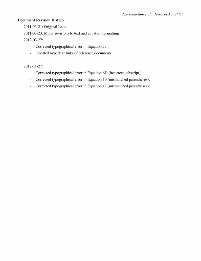
Document Revision History2011-03-21: Original Issue2011-08-23: Minor revisions to text and equation formatting2012-03-27:

- Corrected typographical error in Equation 7;- Updated hypertext links of reference documents.

2012-11-27:- Corrected typographical error in Equation 6D (incorrect subscript);- Corrected typographical error in Equation 10 (mismatched parentheses);- Corrected typographical error in Equation 12 (mismatched parentheses);


the inductance of a helix of any pitch - electron...

Documents