the influence of deflators on valuation - uv

The Influence of Deflators on Valuation

ABSTRACT

This paper deals with the analysis of the scale effect in the value-relevance of accounting

numbers. We examine different deflators that have been widely used to mitigate such effect.

We demonstrate from both theoretical and empirical viewpoints that most of the usual

deflators employed in the literature generate endogeneity problems. In this paper we propose a

new solution for the scale effect problem in the context of the Ohlson model and based on the

use of exogenous deflators. This alternative produces, at least for the USA and Canada, better

statistical results than endogenous deflators such as the market value, the book value of equity

or the total assets. We claim in the paper that, using the number of employees (size of

workforce of a firm) as deflator, the original relationship in the regression model is not

altered, allowing us to correctly interpret the coefficients associated to book value and

earnings.

Keywords: Scale effect, deflator, employees, value-relevance.

JEL Classification: M41.

* The first named author gratefully acknowledges financial support from the Ministerio de Ciencia y Tecnologia

(SEC2005-07657, Spain).

1

1. INTRODUCTION

This study examines issues related to scale effects in value-relevance empirical models.

Following the Ohlson (1995) framework, numerous studies have investigated the relation

between the market value of equity and accounting variables, basically book value and

earnings. In cross-sectional regressions, variables are affected by differences between sample

firms, so that large (small) firms often have large (small) values of the relevant variables but

these differences are not of research interest. Following Easton and Sommers (2003, p. 25-

26), “the overwhelming influence of large firms in these regressions is referred to as the scale

effect. (…) Therefore the results of the regressions are driven by a relatively small subset of

the very largest firms in the sample”. These scale differences can affect the regression results,

causing heteroscedasticity, coefficient bias and an upwardly biased R-squared.

Previous studies have proposed different solutions to scale problems, essentially to

deflate regression equations by a proxy of the scale or to include a scale proxy as an

independent variable. However, there is no unique solution to this problem, as different

studies propose different methods. Barth and Kallapur (1996) find that including a scale proxy

as an independent variable is more effective than deflation at mitigating coefficient bias, since

deflation can worsen coefficient bias and reduce estimation efficiency. However, a drawback

of this approach is that their findings are sensitive to the scale proxy chosen.

Concerning the use of deflation, common deflators employed in previous studies are

total assets, book value, earnings, number of shares and market value. Christie (1987) argues

that opening market value is the natural deflator. Easton (1998) suggests book value as a more

suitable deflator. Brown et al. (1999) show that the number of shares is not a good deflator, as

it is an arbitrary choice made by the firm that reveals new size differences. They assert,

however, that the opening market value can reduce scale effect. Lo and Lys (2000) discuss

past applications of the Ohlson’s (1995) model and, specifically, they draw attention to the

2

possibility that the proposal solutions may change the nature of the relation, although they

also suggest opening market value as a suitable deflator. Equally, Easton and Sommers (2003)

identify scale with market capitalization and support the use of this variable as a deflator.

Akbar and Stark (2003) find that market value is not a superior deflator in valuation equations

on UK data, as different deflators appear to have similar effects; while Livnat (2000) states

that other variables could be equally good or even better in reducing scale effects. In this line,

Barth and Clinch (2005) find that the number of shares outstanding is generally more effective

at mitigating scale effects, though they recognise that it is difficult to identify which type of

scale effect is present in the data.

Consequently, there seems to be no agreement about the methodology to be adopted to

reduce scale effect problems. Moreover, several studies with the same research objective

arrive at contradictory conclusions.

On the other hand, Brown et al. (1999) find evidence that the increasing value relevance

of accounting over time showed in Collins et. al. (1997) and Francis and Schipper (1999) are

attributable to scale. After controlling its effect, however, value relevance declines. Also Lo

and Lys (2000) assert that most valuation studies draw inappropriate conclusions due to scale

effects. Barth and Clinch (2005) find that scale effects do not simply result from size

differences across firms, as they are unobservable and can be manifest in several ways.

Therefore, new evidence is necessary in order to reduce the pervasive effect of scale and

to draw correct inference in the relation between market value of equity and accounting

variables. The aim of this study is to show if the use of those commonly proposed deflators is

appropriate for reducing the scale effect or if, alternatively, a better deflator for the Ohlson’s

(1995) model exists. In particular, we look at a pool of candidates of deflators and then, select

the “best” one according to various statistical criteria.

3

Our study provides theoretical and empirical evidence of the superiority of using an

exogenous deflator such as the number of employees, that is, the size of the workforce of a

firm. It provides better results in statistical terms than other deflators because this variable is

related to scale and is exogenous in the Ohlson model, so that it avoids the endogeneity

problems associated with other deflators.

The remainder of the paper is structured as follows. In Section 2, we discuss from a

theoretical viewpoint the influence on valuation of different deflators proposed in previous

research. Section 3 is devoted to the sample used in the empirical work. Section 4 presents the

results of the empirical analysis, and finally Section 5 concludes the paper.

2. INFLUENCE OF DIFFERENT DEFLATORS ON VALUATION

In the empirical literature concerning the value-relevance of accounting numbers, most studies

are based in Ohlson’s (1995) framework, and use regression models of the market value of

equity on accounting variables:

...,,2,1,210 =+++= txbvV tttt εααα (1)

where Vt is the market value of a given firm at period of time t; bvt is the book value of equity

at period t, and xt represents accounting earnings from period t-1 to t.

One of the important issues in the above regression is to identify and mitigate the so-

called "scale effect", which arises through the cross-sectional scale differences between

sample firms. Note that the nature of the data we usually encounter in market valuation is such

that the results of regression (1) are generally driven by a relatively small subset of the very

largest firms in the sample. Previous studies have showed that the scale effect produces biases

in the estimated coefficients and heteroscedasticity, leading to model inefficiency. Barth and

Kallapur (1996), Barth and Clinch (2005), Brown et al. (1999), Lo and Lys (2000) and Easton

and Sommers (2003) are some of the studies pointing out scale effects in accounting research.

4

From an econometric viewpoint, let us first consider the cross-sectional counterpart of

equation (1),

,210 iiii xbvV εβββ +++= (2)

where Vi, bvi and xi correspond to the same variables as in equation (1) for a given firm, and

are in fact unobservable, and i

ε has zero mean and constant variance, σ2. As in Barth and

Kallapur (1996), we suppose that the observable variables are ,V*i *

ibv and *ix , which are

related to the unobservable ones in (2) throughout the unknown scale factor Si, which has a

multiplicative effect on the observable variables. That is,

ii*i VSV = ,

ii*i Sbv bv=

and

.Sx ii*i x=

Multiplying both sides in equation (2) by the scale factor Si, we get,

,**2

*10

*iiiii

xbvSV εβββ +++= (3)

with ,*iii Sεε = which is a feasible regression, though with heteroscedastic residuals since the

variance of the error term is proportional to the square of the scale factor Si, i.e., Var( *iε ) =

σ2 Si

2. Barth and Kallapur (1996) also point out that the estimation of the β-coefficients if no

scale factor is taken into account leads to a coefficient bias problem, with the magnitude of the

bias depending on Si. When the true scale factor Si is known, the scale effect is clearly

removed by deflating (3) by Si and thus, getting back to equation (2). However, in practice,

the scale factor is unknown and a proxy has to be found and used to deflate the model. Note,

however, that if we use an incorrect deflator (say Zi) in (3), the error term will still present

heteroscedasticity problems unless the deflator is directly proportional to the true one, i.e., Zi

5

= αSi, for a given α. In such a case, the variance of the error term remains constant (V(εi*/Zi) =

σ2Si

2/Zi

2 = σ

2/α

2) and then standard regression techniques can be applied. In the Ohlson’s

(1995) framework, the deflators usually employed are the number of shares, the market value,

the book value of equity, and the total assets. In most of the empirical papers, authors use

lagged deflators so that the dependent variable is set in terms of market profitability.

2.1. Deflator’s choice

Accounting literature has showed the importance of accounting information for equity

valuation.1 Investors take into account earning information for equity valuation and this fact

generates endogeneity problems if researchers use market value as a deflator in Ohlson’s

(1995) model.

We develop a simple model that is useful to analyze the relationship between the price

of a firm and accounting numbers, specifically earnings. Consider a firm that finances its

investments with retained earnings. Dividends (Dt) are equal to earnings (Xt) plus depreciation

(DPt) minus investment outlays (It), i.e., t t t t

D X DP I= + − , where Xt is properly defined as

earnings after depreciation, interest, taxes and preferred dividends but before extraordinary

items.

Suppose that at time t, expected depreciation and investment at time t + k are

proportional to expected future earnings, that is,

[ ] [ ] ( )1 21t t k t t k t k t k t t k

E D E X DP I E X a a+ + + + += + − = + − ,

where 1a and 2a are the proportionality factors. If we assume a constant discount rate ( r ) for

expected dividends, the market value of equity2 at time t is:

1 Collins and Kothari (1989) and Collins et al. (1997) are two of most cited studies showing the importance of

earnings on equity valuation. 2 Fama and French (1995) used this simple model to establish the relation between book-to-market-equity and

expected stock return, and between book-to-market-equity and earnings on book equity.

6

( )[ ]

( )1 2

1

11

t t k

t kk

E XV a a

r

∞+

=

= + −+

∑ .

This model is very convenient if we want to show the influence of accounting numbers

on the market value of a firm. Let the estimated flows of earnings be formed in such a way

that they grow at the inflation rate g. Then, the market value of firm A is:

( )

( )

1

1 20 1 2

1

1 (1 )( ) (1 )

1

k

kk

g a aV A a a if r g

r gr

x x−

∞

=

+ + −= + − = >

−+∑ ,

and the share price is equal to:

( )1 2

0

(1 )( )

a aP A

r g N

x+ −=

−,

where N is the number of shares.

We observe from the above framework that the market value depends on earnings and,

if we use it as a deflator, it would alter the information contained in earnings and book value.

We need a cross-sectional constant to maintain the proportionality relation between market

value and earnings; however market value is not a constant term, as it depends on earnings. So

this deflator would not be a good solution for the scale effect because it would not maintain

the original relationship between market value and earnings. Coming back to the Ohlson’s

(1995) model, which is described through the relationship,

0 1 2t t tV bv xα α α= + + , (4)

and supposing that in period 1, 1 0 (1 )V V k= + , if we deflate the model in period 1 by market

value in period 0, we obtain:

' ' '10 1 2

1 1

0 0 0

V

V V V

xbvα α α= + + .

Noting that 1

x x= , 1

d d= , and 1 Cbv x d= + − , where C is the initial and unique contribution,

then,

7

( ) ( )

' ' '

0 1 21 2 1 2

0

0

(1 )

(1 ) (1 )

k C

a a a a

r g r g

V x d xx xV

α α α+ +

+ − + −

− −

−= + +

( )( ) ( )' ' '

0 1 2

1 2 1 2

(1 )(1 ) (1 )

C r g r gk

a a a a

x d

xα α α

+ − −+

+ − + −

−= + +

( ) ( )' ' '

0 1 2

1 2

(1 )(1 )

Cr gk

a a

x d

xα α α

+− +

+ −

−= + +

( ) ( ) ( ) ( )' ' ' ' '0 1 2 1 0 1

1 2 1 2

''(1 )(1 ) (1 )

r g C d C d r gk

a a a ax xα α α α α α

− − − −+ =

+ − + − = + + + + (5)

being ( )'' ' ' '

0 0 1 21 2(1 )

r g

a aα α α α

− = + −

+ + .

We clearly see that the final relationship in (5) is not the original one, because this

deflator has altered the relation between accounting numbers and the return.

On the other hand, the number of shares is neither a good solution for the scale effect

because it is arbitrary and sometimes has no relation with the size of a firm. Let us consider

the case of two firms with the same accounting numbers and market value but where one of

the firms has one share and the other has a large number of shares. Then, we would clearly

have a scale effect problem in the regression model (1).

Next, we analyze the book value of equity as a potential deflator. We consider a firm

that finances its investments with retained earnings. In this context, we define the book value

of equity at period t as

( )1 1

t t

t k k

k k

bv A C X D= =

= + −∑ ∑ ,

where C is the initial contribution of shareholders, Xk earnings in period k and Dk is all the

pay-out in period k. We define k k k k

D X DP I= + − . Therefore the book value is:

( )1 1 1

( ) ( )t t t

t k k k k k k

k k k

bv A C X X DP I C I DP= = =

= + − + − = + −∑ ∑ ∑ .

8

Noting that 0bv C= and 1

x x= , if we deflate equation (4) by the book value in period

0, we obtain:

' ' '10 1 2

1 1

0 0 0bv bv bv

V xbvα α α= + +

' ' '1 10 1 2

1 ( )C I DP

C C C

V xα α α+ −= + +

( )1 1' ' ' '

0 1 1 21 I DP

C C C

V xα α α α−

+= + + . (6)

As in the previous case, the relation in (6) is different from the original one, and thus,

the book value of equity is neither a good deflator because it also alters the original

relationship.

Finally, the level of total net assets of a firm has also been used in the literature as a

potential deflator. We can calculate the total net assets of a firm in year t as follows:

( ) ( )0 1 1

t t t

t k k k k t

k k k

TA I DP C I DP bv A= = =

= − = + − =∑ ∑ ∑ ,

where C = I0. We observe that the total net assets are exactly the same as the book value of

equity if the firm finances its investments with retained earnings. Thus, this deflator would not

be a good solution either.

As mentioned in previous pages, from an econometric viewpoint, two additional issues

still arise in the scale effect problems. On the one hand, cross-sectional scale differences

between sample firms may result in biased coefficient estimates. On the other hand, the scale

differences also produce heteroscedastic regression errors that can cause biased standard error

estimates and inefficient results. These two issues are crucial for the interpretation of the beta-

coefficients in the regression model (1).

In this paper we argue that the number of employees may be a better deflator than the

ones mentioned above since this variable does not affect the original relationship (4), because

9

it is a cross-sectional constant that maintains the proportionality relation between market

value and earnings. Lo and Lys (2000) draw attention to the possibility that solutions

proposed by accounting literature may change the nature of the studied relation. Moreover,

number of employees is a good proxy for the scale, since the number of employees is usually

related to the size of accounting numbers. Actually, it is the size of workforce of a firm. Also,

in other lines of accounting research, this variable has been widely used as a scale proxy. (See,

e.g., Subramanyam and Zhang, 2001, and Hann et al., 2006). Moreover, by using an

exogenous variable in the Ohlson’s (1995) model, as is the case with the number of

employees, we should expect to get more efficient results in the estimation of the coefficients

in the (deflated) regression model.

3. DATA

Our sample consists of annual accounting data over the period 1995-2004. The accounting

information comes from the Global Vantage database. From this source we take into account

data at the end of each fiscal year.

We extract the following data for each firm: common shares outstanding (shares),

number of employees (Emp.), market value (V), common equity (book value –bv-), total

assets (ta), common stock (cs), common stock plus capital surplus (contributions), and

earnings before extraordinary items (earnings-x-). Moreover, as is usual in value-relevance

literature, we only consider non-financial companies, and firms with positive common equity.

That gives a maximum of 21,134 observations for the US capital market and 3,310 for the

Canadian capital market.

3.1. Descriptive statistics

10

Table 1 shows descriptive statistics of the variables in our sample. We observe that all

variables in the USA and Canada move in a very similar way. All selected variables (number

of shares, book value, total assets, common stock and contributions) increase across the

sample in both countries. Market value grows until 2000, then it declines in 2001 and 2002,

and it increases again over 2003 and 2004. This pattern holds for the two analyzed countries,

the USA and Canada.

(Insert Table 1 about here)

For the book-to-market ratio the behavior is slightly different from one country to

another. Thus, for the US, we observe a value of about 0.31. In Canada this ratio is around

0.49. The behavior in the USA and Canada in terms of earnings is practically the same. We

observe that earnings decline in both countries in 1998 and 2001, the only difference is that, in

Canada, in 2001 the earnings mean is negative. We see that for the number of employees the

behavior is very similar too. The only observed difference is that, for the USA in 2000, the

number of employees grows at around 550 employees per firm, while in Canada it diminishes

by around 200 employees per firm.

To sum up, the behavior of all the variables is practically the same in the two financial

markets. This is not at all surprising if we note for instance that Mittoo (1992) found that both

interlisted and non-interlisted Canadian securities are integrated with the US market.

4. EMPIRICAL RESULTS

Which deflator is the best to solve the scale effect problems in accounting numbers is still an

open question. The literature on this topic suggests different methods to solve the scale

problem. Barth and Kallapur (1996) identified the econometric problem created by scale

effects, resulting in biased coefficient estimates and heteroscedastic regression errors. They

consider scale as an omitted variable, and state that in the special case that the scale factor is

11

known, deflation cures coefficient bias and heteroscedasticity, and it would thus be the best

remedy for it. They establish two alternatives for the scale effect problems: to deflate by a

scale proxy, and to include a proxy of the scale as an additional independent variable. They

list total assets, sales, book value, net income, number of shares outstanding and share prices

as proxies for this unknown scale factor. In this line of research, Collins et al. (1997) and

Francis and Schipper (1999) use book value and net income as independent variables for

explaining market capitalization.

Other studies have also showed the benefits of deflating. Christie (1987) concludes

that the correct deflator in return studies is the market value of equity at the beginning of the

year. Easton (1998) proposes book value as deflator. Notwithstanding, Barth and Clinch

(2005) affirm that the number of shares is an effective general proxy of scale and that share-

deflated specifications perform best for data with scale effects. Lo and Lys (2000) use opening

market value and Easton and Sommers (2003) argue that the best deflator is the market value

at the end of fiscal year. However, Akbar and Stark (2003) argue that the deflator proposed by

Easton and Sommers (2003) is not the best deflator when UK data are used.

The argument we employ in this paper is that the deflators used in the above-

mentioned works could partly solve the scale effect problems, but they also generate

endogeneity if we are in the context of the Ohlson’s (1995) model. In that respect, we propose

the use of the number of employees as a proxy to solve the scale effect problem, keeping the

original interpretation of the beta-coefficients in the regression model (1). Moreover, in other

lines of accounting research the number of employees has been widely employed as a proxy

since it is the size of workforce of a firm. Therefore, we expect that using such an exogenous

regressor would also produce more efficient results in the estimated coefficients from the

regression model.

12

4.1. Coefficients

First we evaluate the Ohlson model with different deflators to see if there are differences

between the two countries in the estimated coefficients. The equation, estimated by Ordinary

Least Squares (OLS), is:

0 1 2it it it

it

it it it

V bv

S S S

xβ β β ε= + + + (7)

where it

V is market value of firm i at the end of fiscal year t , it

bv is common equity of

company i in year t , it

x are earnings before extraordinary items of firm i in year t , it

ε is

residual error on firm i in year t , and it

S is the deflator used in the regression to solve the

scale effect problem.

Table 2 shows the estimated coefficients in the regressions, first with no deflation and

then including a variety of them. The most interesting feature observed in this table is that

these coefficients are different depending on the deflator used. This is obvious because the

interpretation is not exactly the same and it clearly depends on the deflator used. We observe

that the coefficients corresponding to book value (β1) and earnings (β2) are closer in the two

countries than the other deflators when the number of employees is used as deflator. Thus, it

seems that this deflator is not strongly influenced by differences across countries.

(Insert Tables 2 and 3 about here)

We also observe several differences in the estimated coefficients across different

deflators. The coefficients corresponding to book value (β1) in the USA vary between 0.30

and 3.76 and they are between 0.29 and 3.20 for Canada. In the case of earnings (β2) the

coefficients vary between 0.94 and 7.65 for the US market and between -0.88 and 3.36 for

Canada. Next, we want to examine if there are scale effect problems in our sample and if, as

Easton and Sommers (2003) postulate, the origin of these problems comes from market value

differences across firms. For this purpose we divide our sample, based on the size of the

13

workforce (number of employees), into 60 groups in the US market and 10 groups in Canada,

maintaining the proportion observed in our sample size. In Table 3 we display the Spearman

correlation coefficients between the variables in the Ohlson model. It can be seen that the

portfolio with the highest number of employees has the highest correlations. Also, if we

observe the correlation taking into account all observations in the sample pool, we see that

this correlation is highly influenced by the portfolio with the highest number of employees,

P60 for the US firms and P10 for the Canadian ones. This is clear in the case of the correlation

between market value-earnings and earnings-book value. Also noticeable is the fact that the

mean value of all portfolios is always lower than in the pool of observations, indicating

thereby that there is a scale effect problem. We observe that the portfolio with the largest

firms (in workforce terms) has a number of employees three times higher than the preceding

portfolio.3 Also, we observe that the difference in size between the portfolio with the largest

and the smallest size is similar in the two countries. Therefore, the large difference between

size portfolios is the origin of the scale effect problem, and the US market seems to present

similar scale-related problems to the Canadian market.

The follow-up step in this direction is to compare the results using different deflators

to resolve the scale effects, taking into account that some deflators might be related to the

variables in the Ohlson model, and thereby, as showed in Section 2, possibly generating

severe endogeneity problems.

4.3. Residuals

In line with the results displayed in the preceding section, we next show that the scale effect

problems do not simply result from market value differences between firms since scale may

have several other dimensions. We form 60 portfolios for the USA and 10 for Canada, within

3 Similar results are obtained when we construct portfolios by market value.

14

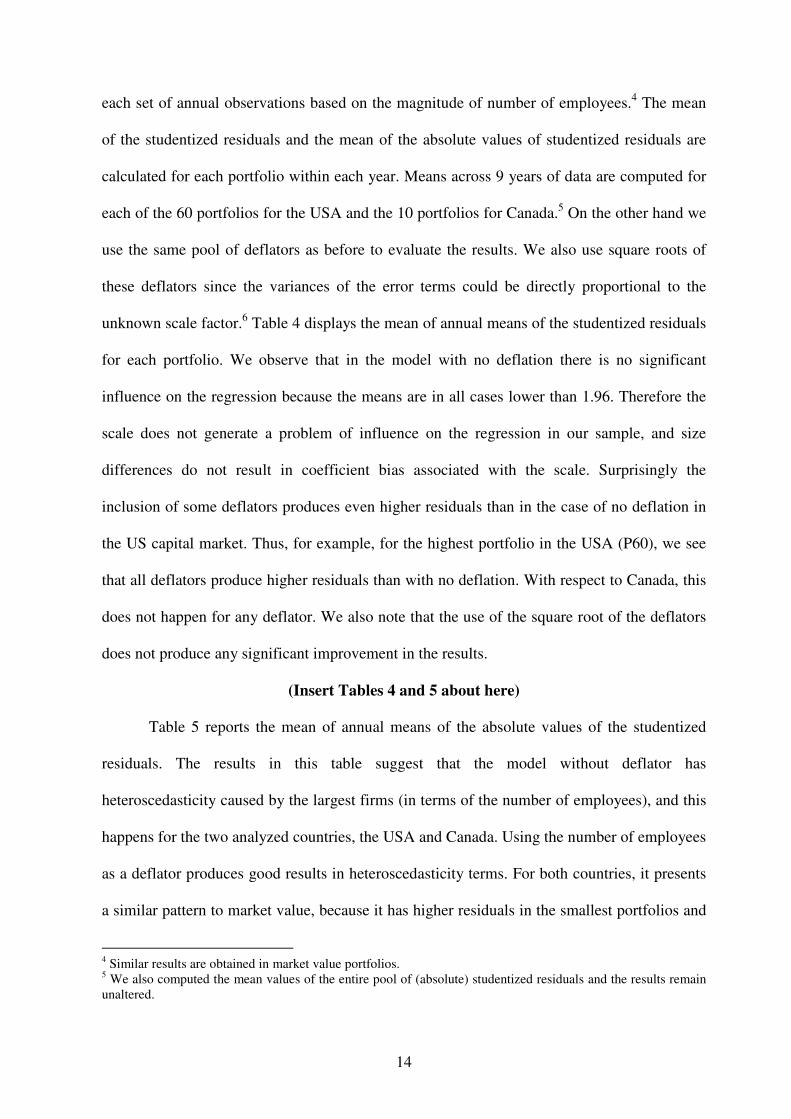
each set of annual observations based on the magnitude of number of employees.4 The mean

of the studentized residuals and the mean of the absolute values of studentized residuals are

calculated for each portfolio within each year. Means across 9 years of data are computed for

each of the 60 portfolios for the USA and the 10 portfolios for Canada.5 On the other hand we

use the same pool of deflators as before to evaluate the results. We also use square roots of

these deflators since the variances of the error terms could be directly proportional to the

unknown scale factor.6 Table 4 displays the mean of annual means of the studentized residuals

for each portfolio. We observe that in the model with no deflation there is no significant

influence on the regression because the means are in all cases lower than 1.96. Therefore the

scale does not generate a problem of influence on the regression in our sample, and size

differences do not result in coefficient bias associated with the scale. Surprisingly the

inclusion of some deflators produces even higher residuals than in the case of no deflation in

the US capital market. Thus, for example, for the highest portfolio in the USA (P60), we see

that all deflators produce higher residuals than with no deflation. With respect to Canada, this

does not happen for any deflator. We also note that the use of the square root of the deflators

does not produce any significant improvement in the results.

(Insert Tables 4 and 5 about here)

Table 5 reports the mean of annual means of the absolute values of the studentized

residuals. The results in this table suggest that the model without deflator has

heteroscedasticity caused by the largest firms (in terms of the number of employees), and this

happens for the two analyzed countries, the USA and Canada. Using the number of employees

as a deflator produces good results in heteroscedasticity terms. For both countries, it presents

a similar pattern to market value, because it has higher residuals in the smallest portfolios and

4 Similar results are obtained in market value portfolios.

5 We also computed the mean values of the entire pool of (absolute) studentized residuals and the results remain

unaltered.

15

lower residuals in the largest ones. The square root version of this deflator produces slightly

better results than the version without any transformation.

So far we have seen that our proposed deflator (and its square root version) corrects

the heteroscedasticity generated by the scale. This solution is recommended by Lo (2005),

among others, who affirms that researchers should generally deflate their models when scale

differences exist in the data. On the other hand, we have been able to show that scale may not

only be due to market capitalization, as Easton and Sommers (2003) affirm, because

constructing portfolios according to the workforce size produces the same scale effects

problems as when forming market value portfolios.

In the following sub-section we consider if the use of the number of employees as

deflator produces smaller prediction errors than those based on models without deflation or

with the other deflators.

4.4. Prediction Errors

We analyze the behavior of the different deflators in terms of their prediction ability. For this

purpose, predictions are obtained from equation (1), then relative prediction errors are

calculated for each observation from the equation:

0 1 2ˆ ˆ ˆit it it

it it it

itit

it

V bv

S S SRPE

V

S

xβ β β

− − −

= , (8)

where variables are defined as in equation (7).


In Table 6 we display the average values of the relative prediction errors across

deflators. All deflators, except the USA Common Stock, improve the results compared with

6 Note that the use of the original variable as a deflator is based upon the assumption that the variance of the error

16

the model with no deflation. The best deflator according to the relative prediction errors is

market value, followed by earnings. The number of employees does also produce good results

in the two analyzed countries. The square root versions of the deflators do not improve the

original deflators in the majority of cases, and thus, they will not be employed in the

forthcoming pages.

4.5. Residual Variance

The variances of the error terms are related to the unknown scale factor. For this reason we

calculate the proportion of the residual variance explained by each deflator. We estimate the

following equation by OLS:

0 1t t tR Sσ β β ε= + + , (9)

where tR

σ is the mean residual variance in year t for the model without deflator, t

S is the

mean of the deflator in year t , and t

ε is residual error in year t .


The regression results were obtained using bootstrap with 9,999 observations in each

regression, repeating this procedure 1,000 times. Table 7 displays the results of the estimated

regression (9), and we observe that the number of employees explains a large proportion of

the variation of the residual variance in the two countries (around 19%). This is consistent

with previous results presented across this paper, verifying that this deflator produces similar

results in the two countries. This is clearly of interest in the sense that we are looking for a

deflator that may not only solve the scale effect problems, but that at the same time, be valid

for global studies. As we observe in Table 7, market value explains around 46% in the USA

but only 1.17% in Canada, implying that this deflator is no good for the latter country. An

term is proportional to the squared variable. (See equation (3)).

17

explanation for that may be related with the standard deviation of market value. It is 66%

higher in the USA than in Canada.

4.6. Endogeneity

We have seen in section 2 that some of the deflators usually employed in the literature

produce serious endogeneity problems. We have also demonstrated that the number of

employees is a good deflator to be used in the context of the Ohlson’s (1995) model, since it

verifies all the conditions for using it properly. Now, we want to prove empirically that the

others deflators used in this paper generate endogeneity as we have previously claimed. For

this reason, we apply Hausman tests comparing equation (1), with a certain deflator, with the

one using the number of employees. In the Hausman test, the null hypothesis postulates

exogeneity while the alternative implies endogeneity of the regressors in the models.


Table 8 shows the results comparing all the deflators with the number of employees.

We see that all null hypotheses are rejected, showing endogeneity problems with the variables

usually employed in the literature. The number of employees seems to be the best deflator,

first because this variable is exogenous, and, as we have demonstrated above, it is also a

useful instrument to solve the scale effect problems in the Ohlson model. Another advantage

of the number of employees is related to the stability of the results obtained with this deflator.

It produces good results in both the US and the Canadian capital markets. Thus it suggests that

this deflator may also be used in other international studies. On the other hand, the Hausman

statistic related to market value is the largest one, implying that although this deflator is good

for correcting heteroscedasticy and for generating estimations in the model, it also generates a

serious problem of endogeneity.

18

5. CONCLUSIONS

In this paper we have examined a number of deflators that have been widely employed in the

empirical literature on value-relevance of accounting numbers to solve the scale effect. We

show that scale effect problems do not simply arise from market value differences across

firms as is claimed for instance by Easton and Sommers (2003). In fact, we have obtained the

same scale effect problems when constructing portfolios according to the number of

employees and by market capitalization, concluding then that the scale has several

dimensions. Moreover, we have shown theoretically, (with a simple model of dividends

supported by accounting and financial literature), and empirically that the deflators most

widely used such as market value, book value of equity or total assets are endogenous in the

context of the Ohlson's (1995) model, leading thus to erroneous interpretations of the

coefficients in the regression model.

In this article we have proposed the use of exogenous deflators in the Ohlson’s (1995)

model. Number of employees seems to be a good deflator as far as this variable, which is

exogenous to the model, does not affect the original relationship between market value of

equity and the accounting variables. Lo and Lys (2000) draw attention to the possibility that

solutions proposed by accounting literature may change the nature of the studied relation.

Number of employees is cross-sectionally constant; therefore it maintains the proportionality

relation between market value and earnings. It is a good proxy for the scale since the number

of employees is usually related with the size of a firm and accounting numbers because it is

the size of workforce. Moreover, it has been widely used in the other lines of accounting

research for controlling by size.

We examined the US and the Canadian markets, and the results, deflated by the

number of employees (and its square root version), outperform the others in the majority of

19

the cases. Furthermore, it produces the closest results between the two markets implying that

it might be more suitable than the others for global studies.

This article can be extended in several directions. First, the number of employees

could be used as a deflator in other empirical studies for other countries, and researchers could

find other deflators to be applied in the Ohlson’s (1995) model, which may also be exogenous

to the model. This is the main contribution of the paper since most widely used deflators in

other works employ variables which are endogenous to the model in the context of value-

relevance accounting numbers.

REFERENCES

Akbar, S. and Stark, A.W. (2003): “Discussion of Scale and the Scale Effect in Market-Based

Accounting Research”, Journal of Business Finance & Accounting, Vol. 30, pp. 57-72.

Barth, M. E. and Clinch, G. (2005): “Scale Effects in Capital Markets-Based Accounting

Research”, Working Paper, Stanford University. University of Technology Sydney.

Barth, M. E. and Kallapur, S. (1996): “The Effects of Cross-Sectional Scale Differences on

Regressions Results in Empirical Accounting Research”, Contemporary Accounting

Research, Vol. 13, Fall, pp. 527-567.

Brown, S., Lo, K. and Lys, T. (1999): “Use of R2 in Accounting Research: Measuring

Changes in Value Relevance over the Last Four Decades”, Journal of Accounting and

Economics, Vol. 28, nº 2, pp. 83-115.

Christie, A. (1987): “On Cross-Sectional Analysis in Accounting Research”, Journal of

Accounting and Economics, Vol. 9, pp. 231-258.

Collins, D., and Kothari, S.P. (1989): “An Analysis of Inter-temporal and Cross-sectional

determinants of Earnings Responsive Coefficients”, Journal of Accounting and Economics,

Vol. 11, pp. 143-181.

Collins, D., Maydew, E. and Weiss, I. (1997): “Changes in the Value Relevance of Earnings

and Book Value Over the Past Forty Years”, Journal of Accounting and Economics, Vol. 24,

pp. 39-67.

Easton, P. (1998): “Discussion of Revalued Financial, Tangible, and Intangible Assets:

Association with Share Prices and Non-Market-Based Value Estimates”, Journal of

Accounting Research, Vol. 36, pp. 235-247.

20

Easton, P. D. and Sommers, G. (2003): “Scale and Scale Effect in Market-Based Accounting

Research”, Journal of Business Finance & Accounting, Vol. 30, pp. 25-55.

Fama, E. and French, K. (1995): “Size and Book-to-Market Factors in Earnings and Returns”,

The Journal of Finance, Vol. 50 (1), pp. 131-155.

Francis, J. and Schipper, K (1999): “Have Financial Statements Lost Their Relevance?”,

Journal of Accounting Research, Vol. 37, pp. 319-352.

Hann, R., Heflin, F. and Subramanyam, K.R. (2006): “Fair-value pension accounting”,

Working Paper, University of Southern California and Florida State University.

Livnat, J. (2000): “Discussion: The Ohlson Model: Contribution to Valuation Theory,

Limitations, and Empirical Applications”, Journal of Accounting, Auditing and Finance, Vol.

15, pp. 368-370.

Lo, K. (2005): “The effects of scale differences on inferences in accounting research:

coefficient estimates, tests of incremental association, and relative value relevance”, Working

Paper, Sauder School of Business.

Lo, K. and Lys, T. (2000): “The Ohlson Model: Contribution to Valuation Theory,

Limitations, and Empirical Applications”, Journal of Accounting, Auditing and Finance, Vol.

15, pp. 337-367.

Mittoo, U.R. (1992): “Additional Evidence on Integration in the Canadian Stock Market”, The

Journal of Finance, Vol. 47, pp. 2035-2054.

Ohlson, J. (1995): “Earnings, Book Values and Dividends in Equity Valuation”,

Contemporary Accounting Research, Vol. 11, pp. 661-687.

Subramanyam, K.R. and Zhang, Y. (2001): “Does stock price reflect future service effects not

included in the projected benefit obligations as defined in SFAS 87 and SFAS 32?”, Working

paper, University of Southern California and Columbia University.

Xu, B. and Wu, C. (2005): “Deflator Selection and Generalized Linear Modelling in Market-

based Accounting Research”, Working Paper, University of Waterloo.

21

Table 1. Descriptive statistics based on the sample. The results in this table are mean values calculated at the end of each fiscal year. Accounting numbers are in US

million dollars for the USA and in Canadian million dollars for Canada. T: Year; Shares: Number of shares by

company (in millions); V: Market value; bv: book value; ta: total assets; Emp.: Number of employees (in

thousands); cs: Common stock; Contrib: Common stock plus capital surplus; Earnings: Earnings before

extraordinary items; Pool: mean value taking into account all observations; N: number of observations.

USA T Shares V bv ta Emp. cs Contrib Earnings

1996 140.09 2,696.04 899.27 4,614.47 11.35 93.11 381.81 143.02

1997 135.18 3,423.70 947.57 4,968.60 11.45 99.58 414.96 148.91

1998 138.74 4,131.56 1,061.00 5,667.59 11.91 109.99 503.68 144.95

1999 142.95 4,945.80 1,206.76 6,379.40 12.35 113.42 594.92 180.40

2000 147.70 5,414.50 1,443.58 7,290.00 12.90 121.07 802.08 189.58

2001 145.89 4,498.97 1,463.30 7,709.80 12.19 118.64 866.88 104.00

2002 152.20 3,770.39 1,501.31 8,404.92 12.69 121.24 992.26 131.19

2003 155.77 4,699.27 1,695.43 9,211.37 12.51 122.86 1,085.53 205.71

2004 198.80 6,630.52 2,494.63 12,827.95 14.55 169.41 1,625.79 328.96

Pool 149.13 4,267.67 1,347.62 7,116.00 12.33 115.36 757.49 167.28

N 21,298 21,193 21,298 21,298 20,846 21,184 21,263 21,286

CANADA Shares V bv ta Emp. cs Contrib Earnings

1996 85.92 1,231.61 659.05 4,304.07 8.37 331.66 358.03 68.43

1997 83.03 1,534.93 694.65 4,805.03 9.38 351.05 367.62 75.02

1998 82.46 1,494.85 755.90 4,981.87 9.62 408.20 426.45 60.13

1999 81.46 2,039.25 783.90 4,834.13 9.85 426.82 442.61 78.01

2000 86.79 2,011.35 947.41 5,743.70 9.65 564.08 595.74 84.46

2001 90.82 1,819.33 918.22 6,399.63 9.49 621.08 657.58 -19.65

2002 103.16 1,647.78 1,020.58 6,977.42 9.81 735.97 771.43 59.97

2003 115.67 2,259.00 1,087.73 7,231.95 8.76 739.71 778.60 121.43

2004 123.82 3,317.28 1,488.45 9,652.35 9.57 807.77 871.16 195.65

Pool 92.38 1,800.19 880.62 5,791.44 9.28 528.56 558.75 72.07

N 3,385 3,325 3,385 3,385 1,539 3,375 3,349 3,373

22

Table 2. Regression results based on different deflators. This equation is estimated by OLS:

0 1 2it it it

it

it it it

V bv

S S S

xβ β β ε= + + +

where it


bv is book value of firm i in year t , it

x are

earnings before extraordinary items of firm i in year t , it

ε is residual error on firm i in year t and it

S is

deflator used in the regression for solving scale effect problem. Deflator column shows deflator used in the

regression. NO: Regression without deflator; Shares: Number of shares outstanding in year t ; V: Market value

in year 1t − ; bv: book value in year 1t − ; ta: Total assets in year 1t − ; Employees: Number of employees in

year t ; cs: Common stock in year 1t − ; Contrib: Common stock plus capital surplus in year 1t − ; Earnings:

Earnings before extraordinary items in year 1t − . * Significant at 10%, ** Significant at 5%, *** Significant at

1%.

USA CANADA

Deflator 0β 1β 2β 2

.adjR N 0β 1β 2β

2

.adjR N

NO 147.50*** 1.82*** 4.66*** 0.82 19,394 82.94*** 1.46*** 1.75*** 0.83 3,034

Shares 9.78*** 0.85*** 3.04*** 0.41 21,134 4.72*** 0.97*** 1.66*** 0.54 3,310

V 0.99*** 0.30*** 1.12*** 0.11 17,943 0.99*** 0.29*** 0.68*** 0.14 2,779

bv -1.12*** 3.76*** 1.56*** 0.22 18,049 -1.11*** 3.20*** -0.88*** 0.24 2,832

ta -0.12*** 2.91*** 2.16*** 0.43 18,049 -0.08** 2.30*** -0.36** 0.43 2,832

Employees 84.18*** 2.17*** 0.94*** 0.60 20,710 1.08 2.09*** 1.29*** 0.76 1,525

cs 183.85*** 2.06*** 1.47*** 0.78 17,956 0.83*** 1.31*** 3.32*** 0.66 2,824

Contrib 1.27*** 1.30*** 7.65*** 0.72 18,019 0.88*** 1.25*** 3.36*** 0.64 2,799

Earnings 0.18 1.88*** 2.61*** 0.68 18,041 -0.63* 1.50*** 1.13*** 0.77 2,822

23

Table 3. Correlations by employees portfolios. This table shows the Spearman coefficient correlation in portfolios classified by size of workforce (number of employees). P1 is the portfolio with the smallest firms and P20 is the

one with the largest assets in number of employees terms. Pool: Correlation taking into account all observations; Mean: Mean value of portfolios; V-bv: Correlation between

market value and book value; V-X: Correlation between market value and earnings; X-bv: Correlation between earnings and book value; Size: Mean number of employees by firm

taking into account all observations.

USA

Pool P1 P2 P3 P4 P5 P6 P7 P8 P9 … P51 P52 P53 P54 P55 P56 P57 P58 P59 P60 Mean

V-bv 0.90 0.69 0.59 0.69 0.75 0.73 0.75 0.77 0.80 0.79 … 0.86 0.85 0.85 0.84 0.86 0.79 0.84 0.87 0.84 0.86 0.80

V-X 0.73 0.11 -0.22 0.04 0.01 0.29 0.11 0.23 0.23 0.23 … 0.78 0.70 0.76 0.83 0.86 0.78 0.86 0.84 0.84 0.87 0.57

X-bv 0.70 0.24 -0.04 0.14 0.10 0.33 0.15 0.25 0.31 0.21 … 0.73 0.67 0.68 0.76 0.78 0.60 0.77 0.72 0.73 0.79 0.52

Size 12.33 0.02 0.05 0.09 0.11 0.14 0.18 0.21 0.25 0.29 … 15.54 17.78 20.82 24.44 29.37 37.15 46.76 61.84 93.33 243.75 12.43

CANADA

Pool P1 P2 P3 P4 P5 P6 P7 P8 P9 P10 Mean

V-bv 0.88 0.75 0.73 0.85 0.74 0.81 0.83 0.94 0.82 0.86 0.90 0.82

V-X 0.64 0.36 0.53 0.63 0.43 0.53 0.65 0.72 0.59 0.65 0.65 0.57

X-bv 0.65 0.46 0.41 0.55 0.41 0.49 0.51 0.68 0.52 0.68 0.66 0.54

Size 9.28 0.06 0.27 0.64 1.22 1.89 2.80 4.41 7.71 18.85 56.46 9.43

24

Table 4. Studentized residuals by employees portfolios. This table shows the mean of annual means of the studentized residuals for each portfolio. P1 is the portfolio with the

smallest firms, in number of employees terms, and P60 and P10 contains the largest ones for the US and Canadian markets

respectively. The residuals are obtained from the estimated equation:

0 1 2it it it

it

it it it

V bv

S S S

xβ β β ε= + + + ,

where it


bv is common equity of company i in year t , it

x are



S is the deflator

used in the regression for solving scale effect problems. Deflator column shows the deflator used in the regression. NO:

Regression without deflator; Shares: Number of shares outstanding in year t ; V: Market value in year 1t − ; bv: Common

equity in year 1t − ; ta: Total assets in year 1t − ; Employees: Number of employees in year t ; cs: Common stock in year

1t − ; Contrib: Common stock plus capital surplus in year 1t − ; Earnings: Earnings before extraordinary items in year

1t − . This table shows the results obtained with the square root version of these deflators too.

USA CANADA

Deflator P1 P2 P3 P4 … P57 P58 P59 P60 P1 P2 … P9 P10

NO -0.03 -0.02 -0.01 -0.01 … 0.31 0.18 0.19 -0.01 0.10 0.09 … -0.44 0.74

Shares -0.35 -0.33 -0.27 -0.11 … 0.68 0.76 0.65 0.89 -0.11 0.03 … 0.19 0.42

V 0.17 0.39 0.23 0.34 … -0.06 -0.05 -0.10 -0.08 0.36 0.13 … -0.06 -0.06

bv 0.37 0.73 0.50 0.56 … 0.20 0.22 0.16 0.38 0.62 0.42 … -0.19 -0.01

ta 0.19 0.63 0.45 0.57 … 0.22 0.22 0.20 0.30 0.54 0.29 … -0.14 0.03

Employees 0.73 0.67 0.39 0.57 … 0.07 0.13 0.07 -0.02 0.39 0.38 … -0.15 0.02

cs 0.00 0.41 0.22 0.36 … -0.06 0.02 -0.15 0.11 0.40 0.37 … -0.24 0.06

Contrib -0.07 0.11 0.04 0.12 … 0.27 0.26 0.31 0.45 0.36 0.37 … -0.25 0.06

Earnings -0.35 -0.50 -0.35 -0.35 … 0.21 0.31 0.23 0.36 -0.20 0.07 … -0.07 0.07

Shares -0.27 -0.14 -0.13 -0.03 … 0.71 0.73 0.71 0.89 -0.06 0.06 … 0.07 0.18

V -0.33 -0.11 -0.10 -0.02 … 0.79 0.87 0.94 1.15 -0.02 0.03 … -0.03 0.44

bv -0.04 0.29 0.20 0.22 … 0.28 0.31 0.34 0.53 0.24 0.31 … -0.22 0.08

ta 0.02 0.36 0.31 0.33 … 0.13 0.15 0.16 0.35 0.36 0.36 … -0.29 0.04

Employees 0.05 0.34 0.19 0.30 … 0.29 0.37 0.29 0.57 0.51 0.25 … -0.31 0.01

cs -0.08 0.09 0.11 0.22 … 0.10 0.13 0.26 0.46 0.09 0.36 … -0.16 0.01

Contrib -0.17 -0.03 -0.03 0.02 … 0.30 0.25 0.31 0.39 0.07 0.37 … -0.17 0.00

Earnings -0.26 -0.20 -0.08 0.01 … 0.37 0.49 0.48 0.62 0.30 0.11 … -0.16 0.22

25

Table 5. Average absolute values of studentized residuals by employees portfolios. This table shows the mean of annual means of the absolute values of the studentized residuals for each portfolio. P1 is the

portfolio with the smallest firms, in number of employees terms, and P60 and P10 contains the largest ones for the US and

Canadian markets respectively. The residuals are obtained from the estimated equation:

0 1 2it it it

it

it it it

V bv

S S S

xβ β β ε= + + + ,

where it



x is



S is the deflator

used in the regression for solving scale effect problems. Deflator column shows the deflator used in the regression. NO:




1t − . This table shows the results obtained with the square root version of these deflators too.

USA CANADA

Deflator P1 P2 P3 P4 … P57 P58 P59 P60 P1 P2 … P9 P10

NO 0.05 0.04 0.05 0.05 … 1.22 1.12 1.68 2.71 0.13 0.18 … 0.83 2.34

Shares 0.84 0.68 0.62 0.63 … 1.01 1.07 1.03 1.15 0.57 0.62 … 0.84 1.04

V 0.96 1.09 0.98 1.00 … 0.55 0.51 0.57 0.51 1.09 0.86 … 0.57 0.55

bv 1.10 1.24 1.03 1.02 … 0.76 0.70 0.69 0.81 1.14 1.11 … 0.61 0.60

ta 1.22 1.34 1.11 1.18 … 0.61 0.60 0.55 0.58 1.28 1.20 … 0.48 0.42

Employees 1.40 1.42 1.21 1.17 … 0.49 0.53 0.47 0.32 1.25 1.15 … 0.29 0.26

cs 0.59 0.78 0.62 0.72 … 0.40 0.48 0.48 0.46 0.67 0.75 … 0.69 0.92

Contrib 0.48 0.51 0.40 0.43 … 0.79 0.73 0.80 0.88 0.62 0.75 … 0.69 0.93

Earnings 0.81 0.80 0.77 0.75 … 0.77 0.68 0.67 0.73 0.83 0.92 … 0.45 0.55

Shares 0.38 0.31 0.29 0.34 … 1.18 1.16 1.29 1.21 0.29 0.43 … 0.99 1.09

V 0.44 0.39 0.39 0.42 … 1.26 1.25 1.44 1.41 0.34 0.49 … 0.90 1.28

bv 0.52 0.60 0.51 0.52 … 1.04 0.92 1.13 1.05 0.45 0.70 … 0.93 1.08

ta 0.54 0.65 0.60 0.61 … 1.02 0.88 1.11 1.08 0.57 0.78 … 0.84 0.99

Employees 0.87 0.73 0.56 0.65 … 0.88 0.86 0.93 1.03 0.89 0.80 … 0.63 0.78

cs 0.49 0.40 0.40 0.53 … 0.71 0.67 0.82 0.94 0.35 0.71 … 0.93 1.04

Contrib 0.29 0.25 0.25 0.30 … 1.01 0.89 1.12 0.97 0.35 0.73 … 0.94 1.03

Earnings 0.39 0.37 0.36 0.38 … 1.13 1.13 1.21 1.13 0.63 0.45 … 0.81 1.18

26

Table 6. Relative prediction errors This table shows relative predictions errors in absolute terms for each deflator used. Predictions are obtained from the

estimated equation:

0 1 2it it it

it

it it it

V bv

S S S

xβ β β ε= + + + ,

where it



x is



S is the deflator

used in the regression for solving scale effect problems. Deflator column shows deflator used in the regression. NO:




1t − . This table shows the results obtained with the square root version of these deflators too. Therefore, relative

prediction errors for each observation are calculated from the equation:

0 1 2ˆ ˆ ˆit it it

it it it

itit

it

V bv

S S SRPE

V

S

xβ β β

− − −

=

Relative prediction errors are average values.

Deflator USA CANADA Deflator USA CANADA

NO 5.23 3.95 Shares 1.83 1.59

Shares 1.52 1.90 V 0.94 0.85

V 0.43 0.45 bv 1.16 1.05

bv 1.01 1.03 ta 1.14 1.12

ta 0.98 1.05 Employees 1.71 1.00

Employees 1.80 0.93 cs 2.50 1.17

Cs 12.16 1.16 Contrib 1.25 1.21

Contrib 1.15 1.18 Earnings 0.86 0.80

Earnings 0.67 0.71

27

Table 7. Residual variance explained by deflator using bootstrap. This table shows beta coefficients and adjusted R-Square for the following regression:

0 1tR t tSσ β β ε= + + ,

where tR

σ is mean residual variance in year t for the model without deflator, t

S is mean of deflator in year t and t

ε is

residual error in year t . Deflator column shows deflator used in the regression. Shares: Number of shares outstanding in

year t ; V: Market value in year 1t − ; bv: Common equity in year 1t − ; ta: Total assets in year 1t − ; Employees:

Number of employees in year t ; cs: Common stock in year 1t − ; Contrib: Common stock plus capital surplus in year

1t − ; Earnings: Earnings before extraordinary items in year 1t − . This regression results have been obtained using

bootstrap with 9,999 observations in each regression, repeating this procedure 1,000 times. * Significant at 10%, **

Significant at 5%, *** Significant at 1%.

USA CANADA

Deflator 0β 1β

2

.adjR 0β 1β

2

.adjR

Shares 5,865.78*** 19.33*** 1.39% 5,815.98*** -37.70*** 10.14%

V 545.61*** 1.84*** 45.89% 1,605.66*** 0.33*** 1.17%

bv 6,271.77*** 1.78*** 7.61% 3,426.48*** -1.27*** 3.09%

ta 6,484.86*** 0.30*** 6.20% 3,974.83*** -0.28*** 6.56%

Employees -9,149.72*** 1,442.37*** 19.06% -12,823.6*** 1,604.64*** 18.45%

cs 2,750.83*** 50,74*** 12.13% 3,464.88*** -2.20*** 4.64%

Contrib 7,277.94*** 1.86*** 5.53% 3,525.38*** -2.19*** 5.28%

Earnings 7,463.77*** 7,53*** 2.47% 2,278.96*** -0.44 0.01%

28

Table 8. Hausman Test This table shows the results of applying Hausman test to the following equations:

1 2it it it

it

it it it

V bv

S S S

xβ β ε= + + ,

1 2it it it

it

it it it

V bv

Employees Employees Employees

xβ β ε= + + ,

where it



x is

earning before extraordinary items of firm i in year t , it


S is the deflator used

in the regression for solving scale effect problems. Shares: Number of shares outstanding in year t ; V: Market value in

year 1t − ; bv: Common equity in year 1t − ; ta: Total assets in year 1t − ; Employees: Number of employees in year t ;

cs: Common stock in year 1t − ; Contrib: Common stock plus capital surplus in year 1t − ; Earning: Earning before

extraordinary items in year 1t − . In Hausman test, the null hypotheses postulates exogeneity while the alternative implies

then endogeneity.

USA CANADA

Comparison (Deflator – Employees)

2χ p-value 2χ p-value

Shares - Employees 2,947.62 .0000 705.17 .0000

V - Employees 10,803.30 .0000 3,526.34 .0000

bv - Employees 504.78 .0000 158.45 .0000

ta - Employees 780.40 .0000 36.28 .0000

cs - Employees 37.06 .0000 197.20 .0000

Contrib - Employees 868.71 .0000 222.28 .0000

Earnings - Employees 266.60 .0000 331.68 .0000

the influence of deflators on valuation - uv

Documents