Loughborough UniversityInstitutional Repository

The influence of hospitalward design on resilience toheat waves: an explorationusing distributed lag models

This item was submitted to Loughborough University's Institutional Repositoryby the/an author.

Citation: IDDON, C.R. ... et al., 2015. The influence of hospital ward designon resilience to heat waves: an exploration using distributed lag models. Energyand Buildings, 86, pp. 573-588.

Additional Information:

• This is an Open Access Article (CC-BY 3.0). It is published by Elsevieras Open Access at: http://dx.doi.org/10.1016/j.enbuild.2014.09.053

Metadata Record: https://dspace.lboro.ac.uk/2134/16610

Version: Published

Publisher: c© The Authors. Published by Elsevier B.V

Rights: This work is made available according to the conditions of the CreativeCommons Attribution 3.0 Unported (CC BY 3.0) licence. Full details of thislicence are available at: http://creativecommons.org/licenses/by/3.0/

Please cite the published version.

Energy and Buildings 86 (2015) 573–588

Contents lists available at ScienceDirect

Energy and Buildings

j ourna l ho me page: www.elsev ier .com/ locate /enbui ld

The influence of hospital ward design on resilience to heat waves:An exploration using distributed lag models

C.R. Iddona,b, T.C. Mills c, R. Giridharand, K.J. Lomasa,∗

a Building Energy Research Group School of Civil and Building Engineering, Loughborough University, LE11 3TU, UKb SE Controls Lancaster House, Wellington Crescent, Fradley Park, Lichfield, Staffordshire WS13 8RZ, UKc School of Business and Economics, Loughborough University, LE11 3TU, UKd Kent School of Architecture, University of Kent, Canterbury CT2 7NZ, UK

a r t i c l e i n f o

Article history:Received 1 May 2014Received in revised form25 September 2014Accepted 26 September 2014Available online 29 October 2014

Keywords:HeatwaveOverheating riskDistributed lag modelsThermal modellingHospitalsResilliancePredictionForecasting

a b s t r a c t

Distributed lag models (DLMs) to predict future internal temperatures have been developed using thehourly weather data and the internal temperatures recorded in eleven spaces on two UK National HealthService (NHS) hospital sites. The ward spaces were in five buildings of very different type and age. In all theDLMs, the best prediction of internal temperature was obtained using three exogenous drivers, previousinternal temperature, external temperature and solar radiation. DLMs were sensitive to the buildings’differences in orientation, thermal mass and shading and were validated by comparing the predictionswith the internal temperatures recorded in the summer of 2012. The results were encouraging, with bothmodelled and recorded data showing good correlation. To understand the resilience of the spaces to heatwaves, the DLMs were fed with weather data recorded during the hot summer of 2006. The Nightingalewards and traditional masonry wards showed remarkable resilience to the hot weather. In contrast, light-weight modular buildings were predicted to overheat dangerously. By recording internal temperaturesfor a short period, DLMs might be created that can forecast future temperatures in many other types ofnaturally ventilated or mixed-mode buildings as a means of assessing overheating risk.

© 2014 The Authors. Published by Elsevier B.V. This is an open access article under the CC BY license(http://creativecommons.org/licenses/by/3.0/).

1. Introduction

In populated areas around the globe, and irrespective of local cli-mate, periods of prolonged and uncharacteristically high externaltemperature (often referred to as ‘heat waves’ though debate overthe specific definition of such events remain) correlate to increasesin localised mortality rates. The heat wave in Quebec 2010 sawa 33% increase in daily death rates [1], and in Brisbane, wherepeople are well accustomed to hot weather, significant increasesin mortality were reported during heat waves between 1996 and2005 [2]. Estimates of over 50,000 extra deaths have been recordedfor the Europe-wide heat wave of 2003, of which 22,080 excessdeaths were reported in England, Wales, France, Italy and Portugal[3]. Episodes of prolonged hot weather have been demonstratedto increase mortality in certain vulnerable demographics, particu-larly the over 80s, and to increase in the number of cardiovasculardeaths in individuals aged 45 years or older [4] whilst in Suzhou,

∗ Corresponding author. Tel.: +44 01509 222615.E-mail address: k.l.lomas@lboro.ac.uk (K.J. Lomas).

China, no significant modifying effect by gender, age or educationallevel was observed on temperature–mortality relationship [5].

The Intergovernmental Panel on Climate Change (IPCC) reportsthat since 1950 there is a medium confidence that there has been aconsistent increase in Warm Spell Duration Index (WSDI),1 an indi-cator of the number and frequency of heat wave events, in NorthernEurope [6–8]. It is likely that heat waves will be longer and moreintense in the future due to a warming climate, though there is somedependency on the parameterisation choice used in models to pre-dict these events [6,9]. Regardless of their predicted frequency andintensity, heat waves will continue to occur and this, in conjunctionwith evidence from past events, has focussed efforts on the meansand methods to reduce the risks of mortality during hot weather.

In England, the Department for Health publishes a yearly heatwave plan [10]. Studies on heat waves in London have demon-strated that although mortality increases during heat waves,hospital admissions do not increase significantly, suggesting that

1 Warm Spell Duration Index (WSDI): fraction of days per year or season whichbelong to periods of at least 6 days at which consecutively Tmax > q90, where q90gives the climatological 90%-quartile of Tmax for that day.

http://dx.doi.org/10.1016/j.enbuild.2014.09.0530378-7788/© 2014 The Authors. Published by Elsevier B.V. This is an open access article under the CC BY license (http://creativecommons.org/licenses/by/3.0/).

574 C.R. Iddon et al. / Energy and Buildings 86 (2015) 573–588

the most vulnerable groups are the elderly living alone or withlimited social contact, and the heat wave plans rightly focus partic-ular attention on these demographics [11].

Hospitals must be resilient to heat waves as they house peo-ple with chronic medical conditions who are thus vulnerable toprolonged high temperature. Proposed measures to reduce mortal-ity risks to patients during heat wave events, include maintaining‘cool’ zones [10,12]. Kravchenko et al., in an American study, recom-mend controlling the internal environment and provision of ‘cool’zones with air conditioning, however the National Health Service(NHS) faces a challenge: how to deliver safe environments in achanging climate whilst meeting ambitious carbon reduction tar-gets. Widespread use of air-conditioning is unlikely to meet bothcriteria [13,14].

Very few hospital wards in the UK are air-conditioned; insteadthe internal temperature is maintained by natural or mechanicalventilation. The summertime internal temperatures in 125 suchspaces, of which 97 were wards, located on four hospital sites,(Addenbrooke’s, Cambridge; Glenfield, Leicester; St. Albans; andBradford Royal Infirmary), were measured as part of the UK project,Design and Delivery of Robust Hospital Environments in a Chang-ing Climate (DeDeRHECC), the largest known UK survey of hospitaltemperatures. These data were then used to calibrate dynamic ther-mal models and the likely overheating during heat wave eventspredicted [14–17]. Thermally lightweight construction was pre-dicted to increase the risk of overheating. Refurbishment optionsto reduce overheating risk and reduce energy demands wereexplored.

This paper capitalises on the DeDeRHECC data but developsempirical models for wards through statistical analysis of mea-sured internal and external temperatures. This approach, whichavoided the errors and uncertainties associated with thermal modelcalibration, led to the creation of a unique distributed lag model(DLMs) for each hospital ward. The DLMs were created using datacollected during the summer of 2011 and validated against datafrom the summer of 2012. The models were then used to predictthe resilience of wards in buildings of different type to an extremelyhot summer; the Europe-wide heat wave of 2006.

1.1. Modelling internal temperature

Previous studies, such as the DeDeRHECC project, have tendedto focus on the development of dynamic thermal models as a way tounderstand the characteristic response of room temperature and toprovide a means of future forecasting. Such models use a buildingphysics approach, in which the salient thermo-physical propertiesof the building are exposed to past or future boundary conditions.Many of the thermo-physical features, and the details of the bound-ary conditions, are unknown and so assumptions must be made.To aid this process, measurements sometimes are used to providedata against which to ‘calibrate’ the model in order to improve thefit between predicted and measured parameters, such as internalair temperature e.g. [14,15,17]. There are however many modelinputs for which assumptions must be made and the final set ofinputs, although ‘valid’ based on the limited knowledge of the sys-tem in question, are just one possible set of inputs that could beselected. Models also embed simplifications, internal heat gains areestimated and specified as simple, repeating daily schedules andreal-world events can often be ignored or grossly simplified, forexample occupant window opening. Thus even ‘calibrated’ mod-els are inherently limited and assumption choice may be biased byknowing the recorded data to which the model should align; themodel therefore loses impartiality [18,19].

An alternative approach to understanding the factors that driveinternal temperatures in a space is to develop purely empiricalmodels which consider the dynamic heat balance of a space which,

at a point in time, can be considered as: heat of a system = heat intoa system – heat lost from the system. The recorded internal tem-peratures provide a snapshot of the dynamic heat energy balanceat work in the space. Comparison of the recorded internal tem-perature at the t=0 and t=−1 time-points allows the elucidation ofwhether the heat energy into the space is greater or less than heatlost from the space over a time period such as an hour. This canprovide an insight into the magnitude of energy into, and out of asystem on an hourly basis, such that; if energy into the system isgreater than that leaving the system, the internal temperature willincrease with respect to the temperature at t=−1.

The difficulty with such an analysis lies in the myriad processesthat affect the space heat balance. These include, but are not limitedto, heat supplied to, or lost from a space via the ventilation sys-tem, through air leakage, from room occupants, through windowopenings, by fabric conduction, by solar radiation, from lightingand small power sources, and, in winter, the heating system. Even acomputer thermal model that has undergone the most rigorous cal-ibration will still not accurately reflect measured temperatures asthere is so much that will never be known with regard to transientinfluences on the internal temperature.

Time series analysis has often been employed with temperaturedata sets, not least because regular diurnal and seasonal trends canbe readily modelled by such analysis. Models have been generatedto: predict external air and solar radiation events [20]; predict theresponse of internal temperature to changes in outside tempera-ture [21]; predict internal temperature for HVAC control systems[22]; to estimate building energy performance by robust regression[23]; and to model climate change [24]. Similar principles are usedin this paper to create a model that can reproduce the inherentfeatures of the internal temperature profiles recorded in hospitalwards.

This paper reports work in which a novel time series modelwas developed to predict the internal temperature at any time, t0,based upon the internal temperature in preceding hours and thedriving exogenous effects of external dry bulb temperature, exter-nal global solar irradiance and external solar irradiance incident onthe plane of the building. Comparing the diurnal internal temper-ature profiles in several spaces as recorded in the summer of 2011,revealed a relationship with room orientation. Using this as a start-ing point, a distributed lag model (DLM) of internal temperaturewas created for each space based on the measured hourly externalweather conditions, and the internal temperatures recorded in eachspace.

1.2. Modelled spaces

As part of the DeDeRHECC project, temperatures were recordedat hourly intervals for between 6 months and 3 years, in 97 wards, in9 hospital buildings, on four sites: Bradford Royal infirmary, Leices-ter Glenfield, Addenbrookes Hospital Cambridge, and St AlbansHospital. This paper focuses on 11 hospital wards in five buildingson the Bradford and St Albans sites. These provide examples of avariety of architectural forms and construction types: a traditional(c1930s), thermally heavyweight, Nightingale building [14,25]; avery modern (2008), thermally lightweight, modular building; andthree 1960s–1970s buildings, two towers – the matchbox of the‘matchbox on a muffin’ building type [17] and a masonry slab build-ing (Table 1). The buildings, with their roughly north-south axisorientation, test the ability of the time series analysis to detect theinfluence of ward orientation, east or west, on space temperatures.Further information regarding the spaces monitored can be foundin the electronic appendix.

Temperature loggers, Hobo type U12-001, were used to recordthe temperatures at hourly intervals, however, the location of each

C.R. Iddon et al. / Energy and Buildings 86 (2015) 573–588 575

Table 1Building types, locations and descriptions ofwardstaken as representative for the building.

Location Ward type Building details Space Refa Space details

Bradford RI Nightingale Built c1927–1937Walls – stone, c.500 mm thick, comprising 150 mm stoneouter skin and 350–400 mm inner skin with some rubbleinfillWindows – thermally broken aluminium-framed doubleglazed unitsVentilation – natural ventilation, opening windows

BNi-W Twin bed ward facing due west270◦ NVolume, 60 m3

Ground floor

Bradford RI Modular Built 2008Walls – lightweight insulated panels U-value 0.2 Wm2 K

BMo-E Single bed roomsFacing due east 90◦ NVolume, 42 m3

Ground floorWindows – double glazed, toughened, low e soft coat,U-value of 1.2 W/m2 KVentilation – mechanical ventilated, supply into rooms,extract via fabric and dedicated extract ducts in toiletareas. Circa 4ach. Windows can be opened to providefurther ventilation.

BMo-W Multi-bed wardsFacing due west 270◦ NVolume, 123 m3

Ground floor

Bradford RI Maternity TowerLinear SlabRooms from ‘matchbox’element of the ‘Matchboxon a Muffin’ type

Built c1965–1967Concrete frame with continuous window ribbonincorporating opaque panelsOpaque panels – Gyproc system with insulated cavity

BMa-E Single bedFacing due east 90◦ NVolume, 35 m3 m4th Floor

Windows – recently replaced double glazed systemVentilation – mechanical ventilated, supply into rooms,extract via fabric and dedicated extract ducts in toiletareas. Circa 4ach. Windows can be opened to providefurther ventilation.

BMa-W Multi-bed ward facing duewest 270◦ NVolume, 150 m3

4th Floor

St Albans Moynihan Building TowerLinear SlabRooms from ‘matchbox’element of the ‘Matchboxon a Muffin’ type

Built circa early 1970sConcrete frame with continuous timber frame ribbonincorporating windows and opaque panels.Opaque panels – painted WBP timber outer sheet with25 mm thick dense mineral fibre insulation panel bondedto inner face.Windows – single glazedVentilation – mechanical ventilated, supply into rooms,extract via fabric and dedicated extract ducts in toiletareas. Circa 4ach. Windows can be opened to providefurther ventilation.

SMa-E Multi-bed ward facing southeasterly 135◦ NVolume, 150 m3

Fifth floor

St Albans TraditionalMasonry slab RuncieBuilding

Built 1983Traditional build, 102 mm brickwork outer skin walling,50 mm cavity air-gap, 50 mm mineral fibre insulation,100 mm thick medium density blockwork.

SMs-Esf Single bed ward facing southeasterly, 135◦ NVolume 30 m3

2nd floorWindows – timber framed, double glazedVentilation – mechanical ventilated, supply into rooms,extract via fabric and dedicated extract ducts in toiletareas. Circa 4ach. Windows can be opened to providefurther ventilation.

SMs-W1gf

SMs-W2gf

SMs-W1sf

SMs-W2sf

Multi bed ward facing northwesterly, 315◦ NVolume 135 m3

Ground and 2nd floor

a Room coding: B – Bradford, S – St Albans; Ni – Nightingale, Mo – Modular, Ms – Masonry slab, and Ma – Matchbox element of a ‘matchbox on a muffin’ type; E – East, W– West; gf – ground floor, sf – second floor.

one was heavily constrained by clinical, and other, considerations.2

The loggers were fixed to the walls in such a way that they could beremoved for data downloading and, if necessary, cleaning (for infec-tion control). They were located as far a possible away from heatsources and other thermal stimuli, which would interfere with theattempt to record a mean space temperature. The loggers, whichrecord spot values on the hour, are quoted as being accurate to±0.35 ◦C, and in pre-trial testing the installed loggers recorded towithin 0.2 K of each other at normal room temperature.

The local meteorological data, hourly external dry bulb temper-ature, and global horizontal solar irradiance were recorded by localweather stations, Bingley for Bradford and Northolt for St Albans.Weather stations set up local to each hospital, as part of the DeDeR-HECC project, were used in the 2012 data set. Values for the solar

2 In general, spaces had two loggers but the data used to generate the models wastaken from just one of these because loggers at the back of rooms had a tendency tobe affected by direct solar gain. However, whichever sensor (or average of the two)was used, a DLM could be generated.

radiation incident (SRI) on the external plane of the wards werecalculated using the procedure described in the appendix text.

Data from 1st May to 30th September 2011 was used to developthe DLM for each ward and data recorded from June to September2012 to test DLMs’ accuracy. Data from other periods is used toillustrate features of the measured data and DLMs’ behaviour.

2. Results

2.1. Average diurnal temperature profiles

To appreciate the diurnal temperature profile at each measure-ment location, the average of all the hourly data at a given hourpoint collected between 1st May and 30th September 2011 wasplotted (i.e. 153 × 24 = 3672 h).

Average daily temperature profiles for the east-facing single bedwards of the modular building (BMo-E) and matchbox tower build-ing (BMa-E), indicate that that these spaces warm in the morningbetween 06:00 and 09:00 and that in the heavily insulated modular

576 C.R. Iddon et al. / Energy and Buildings 86 (2015) 573–588

building (BMo-E) the peak temperature is maintained through thecourse of the afternoon before cooling around 19:00 h whilst thematchbox ward begins to cool earlier (Fig. 1). In contrast, the west-facing wards (BMo-W, BMa-W and BNi) begin to warm around12:00 and reach a peak temperature around 18:00–19:00 afterwhich the spaces begin to cool. Generally, the peak temperature ofsuch west-facing wards is higher than in the east facing spaces, buteast-facing spaces cool more slowly and therefore spend more timeat high temperatures, making them more prone to overheating asdefined by the number of hours over a set threshold temperature.The heavyweight Nightingale ward (BNi-W) displays a muchsmaller diurnal swing in internal temperature (1 K) than the lighterweight matchbox and modular wards (BMa-W, BMo-W); diurnalswing circa 2 K. Similar results, which typify east and west facingwards, were observed in the diurnal profiles recorded in the St.Albans Moynihan Tower and Runcie buildings (results not shown).

Although the average temperatures at each hour illustrate cleardifferences between the east and west facing rooms, there is, ofcourse, very large variability between the individual hourly values.To better account for this variability, and thus to develop a morerobust model of internal temperature variations, the difference intemperatures, �t, from a 48 h moving average are used to definethe ward temperature t0:

�t0 = t0 −(∑23

t=−24t

48

)(1)

The hourly internal temperature in a single bed ward in themodular building at Bradford (BMo-E) and the 48 h moving averagetemperature are illustrated in (Fig. 2)

2.2. Impact of solar radiation on internal temperatures

Plotting the monthly average hourly temperature differencefrom the 48 h mean against the monthly average hourly incidentsolar radiation incident on the glazing of a ward, demonstrated aco-incidence between the increase in internal temperature and theincrease in incident solar radiation (Fig. 3).

During January, where the average monthly solar radiation islow, there is little average diurnal swing in internal room tempera-ture away from the 48 h moving average (Fig. 3A and C). Conversely,in April, the higher incident solar radiation drives up the internaltemperatures (Fig. 3B and D) with the west facing ward BMo-W (B)warming in the late afternoon and the east facing ward (BMo-E)warming in the morning (D). Similar plots to those shown in Fig. 3have been generated for many different months and many wardsin all the building types. All these demonstrate the coordination

Fig. 1. The hourly average internal temperature during the summer of 2011 ineast-facing (BMo-E, BMa-E) and west-facing (BMo-W, BMa-W and BNi-W) wards atBradford Royal Infirmary. Similar results for other spaces at Bradford Royal Infirmaryare given in the electronic appendix.

of increases in internal room temperature with increased incidentsolar radiation. The plots generated for the 21 months from January2010 to September 2011 for wards BMa-E, BMa-W, BNi-W, BMo-Eand BMo-W have been collated into a video file (Video 01), whichcan be viewed in the electronic appendix to this paper.

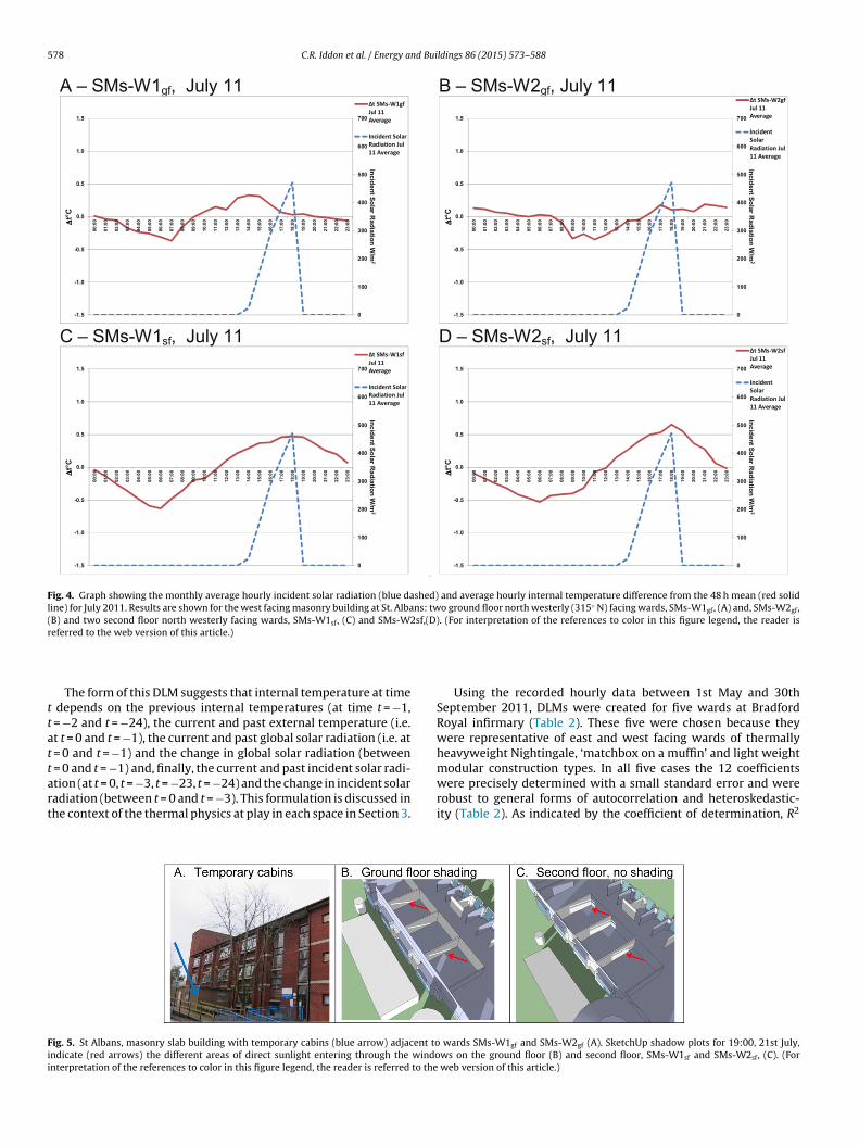
Unexpected results were obtained for the ground floor wardsin the masonry slab building at St. Albans (SMs-W1gf and SMs-W2gf). In these spaces, the internal temperature was insensitiveto the incident solar radiation, yet other west facing wards in thesame building showed the expected sensitivity (Fig. 4A and B, cf.,respectively, 4C and 4D).

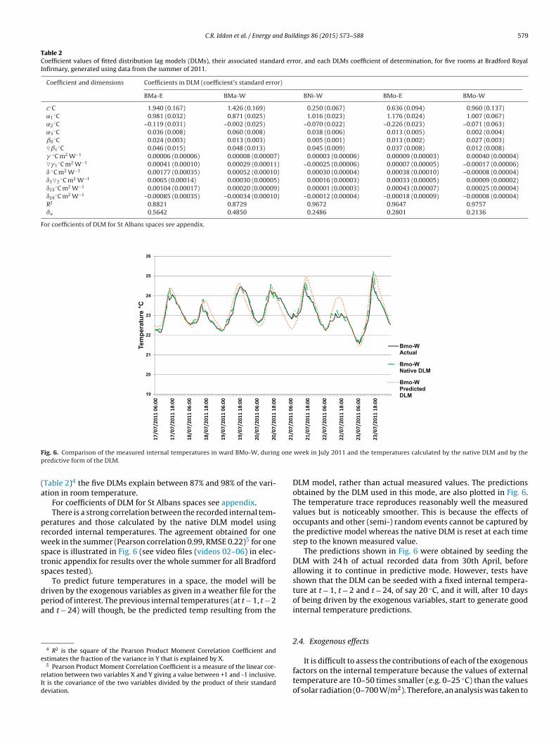
Further investigation (Google imagery and a site visit) revealedthat temporary site cabins had been erected just a few metresfrom the windows on the ground floor wards (Fig. 5A) and GoogleSketchUp (Now Trimble SketchUp) shadow plots confirmed thatthe cabins blocked nearly all direct solar radiation into the groundfloor wards (Fig. 5B) but not into those on the second floor (Fig. 5C).

Monthly average hourly internal temperature versus incidentsolar radiation profiles for other monitored spaces (results notshown) provided evidence for localised shading that decreased theinternal temperature variations. These observations suggest thatsolar gains are one of the most significant factors influencing inter-nal temperature. Therefore, any empirical model to predict internaltemperature must be sensitive to the influence that the local sitetopography has on solar heat gains.

Fig. 2. Hourly internal temperature recorded between 7th June and 9th July 2011, in a single bed ward in the modular building at Bradford Royal Infirmary (BMo-E), showingthe 48 h moving average. The ‘noise’ of the raw temperature data is evident as positive and negative spikes and is due to sudden changes in the space heat balance, due mostlikely to occupant events (such as opening the windows) or transient heat gains (from solar gain or occupants).

C.R. Iddon et al. / Energy and Buildings 86 (2015) 573–588 577

Fig. 3. Graphs showing the monthly diurnal average incident solar radiation (blue dash line) and internal �t (red solid line) during January and April 2011. Modular multibedward facing west (BMo-W) during January (A) and April (B). Modular single bed ward facing east (BMo-E) during January (C) and April (D). (For interpretation of the referencesto color in this figure legend, the reader is referred to the web version of this article.)

2.3. Time series analysis

In light of the suggested correlation between internal tempera-ture and incident solar radiation a time series approach was usedto try and create a model that reproduced the recorded response ofthe internal temperature to three exogenous effects, namely, exter-nal dry bulb temperature, global solar irradiance and incident solarradiation.

Denoting the room temperature as Tt, external temperature asText, global solar irradiation as Sglobal and incident solar radiation asSincident, a distributed lag model (DLM) was developed:

Tt = c +p∑

i=0

˛iTt−1−i +p∑

i=0

ˇiTextt−i+

p∑i=0

�iSglobalt−i

+p∑

i=0

ıiSincidentt−i+ ui (2)

Herein, ut is an error term that is assumed to be identically andindependently distributed as N(0, �2

u ) and the room temperatureat time t is assumed to be a linear function of past lags of itself andcurrent and past lags of the three exogenous variables. This specifi-cation is an example of the traditional econometric autoregressiveDLM, e.g. [26], in which the order of the lags are selected to ensurethat all dynamic effects are accounted for and no autocorrelationremains in the error term.

After some experimentation with the lag structure, usingEViews software ([27] EViews, 2013), and by re-expressing vari-ables to facilitate easier interpretation, the following general modelwas selected3 as providing an adequate fit for each of the roomsmodelled:

Tt = c + ˛1Tt−1 + ˛2Tt−2 + ˛3Tt−24 + ˇ0Textt + ˇ1∇Textt

+(�0 + �1)Sglobalt + �1∇Sglobalt + (ı0 + ı3)Sincidentt

+ı3∇3Sincidentt+ ı23Sincidentt−23

+ ı24Sincidentt−24+ ut (3)

In this equation regressors have been combined to aid interpre-tation (essentially level and change effects have been emphasised:generically: ∇kXt = Xt = Xt−k). Textt represents the external temper-ature at time t in ◦C; Sglobalt represents the global horizontal solarradiation at time t in W/m2; Sincidentt

represents the solar radiationincident to the fac ade of the space at time t in W/m2; Tt−i repre-sents the past internal room temperature at time t − i in ◦C; ˛, ˇ,� and ı are the coefficients related to internal temperature, exter-nal temperature, global solar radiation and incident solar radiationrespectively; and c is a constant.

3 ‘Selected’ here means: selected as the best ‘general’ model to fit all data, to createa model that could be applied to all spaces.

578 C.R. Iddon et al. / Energy and Buildings 86 (2015) 573–588

Fig. 4. Graph showing the monthly average hourly incident solar radiation (blue dashed) and average hourly internal temperature difference from the 48 h mean (red solidline) for July 2011. Results are shown for the west facing masonry building at St. Albans: two ground floor north westerly (315◦ N) facing wards, SMs-W1gf, (A) and, SMs-W2gf,(B) and two second floor north westerly facing wards, SMs-W1sf, (C) and SMs-W2sf,(D). (For interpretation of the references to color in this figure legend, the reader isreferred to the web version of this article.)

The form of this DLM suggests that internal temperature at timet depends on the previous internal temperatures (at time t = −1,t = −2 and t = −24), the current and past external temperature (i.e.at t = 0 and t = −1), the current and past global solar radiation (i.e. att = 0 and t = −1) and the change in global solar radiation (betweent = 0 and t = −1) and, finally, the current and past incident solar radi-ation (at t = 0, t = −3, t = −23, t = −24) and the change in incident solarradiation (between t = 0 and t = −3). This formulation is discussed inthe context of the thermal physics at play in each space in Section 3.

Using the recorded hourly data between 1st May and 30thSeptember 2011, DLMs were created for five wards at BradfordRoyal infirmary (Table 2). These five were chosen because theywere representative of east and west facing wards of thermallyheavyweight Nightingale, ‘matchbox on a muffin’ and light weightmodular construction types. In all five cases the 12 coefficientswere precisely determined with a small standard error and wererobust to general forms of autocorrelation and heteroskedastic-ity (Table 2). As indicated by the coefficient of determination, R2

Fig. 5. St Albans, masonry slab building with temporary cabins (blue arrow) adjacent to wards SMs-W1gf and SMs-W2gf (A). SketchUp shadow plots for 19:00, 21st July,indicate (red arrows) the different areas of direct sunlight entering through the windows on the ground floor (B) and second floor, SMs-W1sf and SMs-W2sf, (C). (Forinterpretation of the references to color in this figure legend, the reader is referred to the web version of this article.)

C.R. Iddon et al. / Energy and Buildings 86 (2015) 573–588 579

Table 2Coefficient values of fitted distribution lag models (DLMs), their associated standard error, and each DLMs coefficient of determination, for five rooms at Bradford RoyalInfirmary, generated using data from the summer of 2011.

Coefficient and dimensions Coefficients in DLM (coefficient’s standard error)

BMa-E BMa-W BNi-W BMo-E BMo-W

c◦C 1.940 (0.167) 1.426 (0.169) 0.250 (0.067) 0.636 (0.094) 0.960 (0.137)˛1

◦C 0.981 (0.032) 0.871 (0.025) 1.016 (0.023) 1.176 (0.024) 1.007 (0.067)˛2

◦C –0.119 (0.031) –0.002 (0.025) –0.070 (0.022) –0.226 (0.023) –0.071 (0.063)˛3

◦C 0.036 (0.008) 0.060 (0.008) 0.038 (0.006) 0.013 (0.005) 0.002 (0.004)ˇ0

◦C 0.024 (0.003) 0.013 (0.003) 0.005 (0.001) 0.013 (0.002) 0.027 (0.003)�ˇ1

◦C 0.046 (0.015) 0.048 (0.013) 0.045 (0.009) 0.037 (0.008) 0.012 (0.008)� ◦C m2 W−1 0.00006 (0.00006) 0.00008 (0.00007) 0.00003 (0.00006) 0.00009 (0.00003) 0.00040 (0.00004)��1

◦C m2 W−1 0.00041 (0.00010) 0.00029 (0.00011) –0.00025 (0.00006) 0.00007 (0.00005) –0.00017 (0.00006)ı ◦C m2 W−1 0.00177 (0.00035) 0.00052 (0.00010) 0.00030 (0.00004) 0.00038 (0.00010) –0.00008 (0.00004)ı3�3

◦C m2 W−1 0.0065 (0.00014) 0.00030 (0.00005) 0.00016 (0.00003) 0.00033 (0.00005) 0.00009 (0.00002)ı23

◦C m2 W−1 0.00104 (0.00017) 0.00020 (0.00009) 0.00001 (0.00003) 0.00043 (0.00007) 0.00025 (0.00004)ı24

◦C m2 W−1 –0.00085 (0.00035) –0.00034 (0.00010) –0.00012 (0.00004) –0.00018 (0.00009) –0.00008 (0.00004)R2 0.8821 0.8729 0.9672 0.9647 0.9757�u 0.5642 0.4850 0.2486 0.2801 0.2136

For coefficients of DLM for St Albans spaces see appendix.

Fig. 6. Comparison of the measured internal temperatures in ward BMo-W, during one week in July 2011 and the temperatures calculated by the native DLM and by thepredictive form of the DLM.

(Table 2)4 the five DLMs explain between 87% and 98% of the vari-ation in room temperature.

For coefficients of DLM for St Albans spaces see appendix.There is a strong correlation between the recorded internal tem-

peratures and those calculated by the native DLM model usingrecorded internal temperatures. The agreement obtained for oneweek in the summer (Pearson correlation 0.99, RMSE 0.22)5 for onespace is illustrated in Fig. 6 (see video files (videos 02–06) in elec-tronic appendix for results over the whole summer for all Bradfordspaces tested).

To predict future temperatures in a space, the model will bedriven by the exogenous variables as given in a weather file for theperiod of interest. The previous internal temperatures (at t − 1, t − 2and t − 24) will though, be the predicted temp resulting from the

4 R2 is the square of the Pearson Product Moment Correlation Coefficient andestimates the fraction of the variance in Y that is explained by X.

5 Pearson Product Moment Correlation Coefficient is a measure of the linear cor-relation between two variables X and Y giving a value between +1 and -1 inclusive.It is the covariance of the two variables divided by the product of their standarddeviation.

DLM model, rather than actual measured values. The predictionsobtained by the DLM used in this mode, are also plotted in Fig. 6.The temperature trace reproduces reasonably well the measuredvalues but is noticeably smoother. This is because the effects ofoccupants and other (semi-) random events cannot be captured bythe predictive model whereas the native DLM is reset at each timestep to the known measured value.

The predictions shown in Fig. 6 were obtained by seeding theDLM with 24 h of actual recorded data from 30th April, beforeallowing it to continue in predictive mode. However, tests haveshown that the DLM can be seeded with a fixed internal tempera-ture at t − 1, t − 2 and t − 24, of say 20 ◦C, and it will, after 10 daysof being driven by the exogenous variables, start to generate goodinternal temperature predictions.

2.4. Exogenous effects

It is difficult to assess the contributions of each of the exogenousfactors on the internal temperature because the values of externaltemperature are 10–50 times smaller (e.g. 0–25 ◦C) than the valuesof solar radiation (0–700 W/m2). Therefore, an analysis was taken to

580 C.R. Iddon et al. / Energy and Buildings 86 (2015) 573–588

Table 3Calculating the monthly average hourly effect of the exogenous variables on the room temperature.

Contribution of previous internal temperatures

∑j

1˛1Tt−1+˛2Tt−2+˛3Tt−24

j

Contribution of external temperature

∑j

1ˇ0Textt +ˇ1∇Textt

j

Contribution of global solar radiation

∑j

1(�0+�1)Sglobalt

+�1∇Sglobalt

j

Contribution of incident solar radiation

∑j

1(ı0+ı3)Sincidentt

+ı3∇3Sincidentt+ı23Sincidentt−23

+ı24Sincidentt−24j

j = number of days in the month.

calculate the monthly average hour contribution of each exogenousdriver to the DLM of each ward (Table 3).

The resulting hourly contributions averaged for June 2011(Fig. 7) demonstrate that the most important contributor is theprevious room temperatures, with values circa 22 ◦C, compared tothe contribution from the exogenous drivers (external tempera-ture, global solar radiation and incident solar radiation), which eachcontribute between −0.2 ◦C and 0.8 ◦C.

There are clear differences in the contribution of the exogenousvariables depending on the building type. Most obviously, the con-tributions of solar radiation and external temperature to the inter-nal temperature in the Nightingale ward (Fig. 7B) are much lowerthan for the other wards. This perhaps reflects the heavyweightnature of the Nightingale structure which is known to attenuate theeffects of external influences. The results also demonstrate that the

incident solar radiation is important in establishing the differentdiurnal profiles observed in rooms of different orientation (west,Fig. 7A; east, Fig. 7C); this was hypothesised with regard to Fig. 1.

Interestingly, this analysis shows that for BMo-W, Fig. 7D, thecontribution of incident solar radiation to internal room tempera-ture after 18:00 h is zero or less. This correlates with the time whenthe building is shaded of an adjacent building. (A SketchUp shadowcast model showed that the timing of the shading in fact variedthrough the year: from 17:00 h in June to 14:00 h in December.)

To further investigate DLMs’ ability to identify shading effects,a summertime model was developed for wards in the tower build-ing at St Albans. One ward, SMa-E, was orientated to the southeast (135◦) with a circa 3.2 m overhang located above the window.SketchUp models predicted that this overhang would block inci-dent solar radiation falling on the room fac ade after 10:00 during

Fig. 7. Monthly average hourly contribution of the exogenous drivers to internal room temperature in June 2011 as indicated by the DLM for four spaces at Bradford RoyalInfirmary: exogenous variables, lh axis, previous internal temperatures, rh axis.

C.R. Iddon et al. / Energy and Buildings 86 (2015) 573–588 581

Table 4Comparison of the correlations between the measured internal temperatures and the temperatures calculated by both the native DLM and the predictive DLM: five wardsall at Bradford Royal Infirmary, during the summer of 2011.

BMa-E BMa-W BNi-W BMo-E BMo-W

RMSE R2 RMSE R2 RMSE R2 RMSE R2 RMSE R2

Native DLM 0.75 0.82 0.48 0.90 0.24 0.96 0.29 0.97 0.22 0.97Predictive DLM 1.73 0.31 1.20 0.37 1.07 0.17 1.34 0.35 0.98 0.59

Table 5Comparison of the measured hours over 25 ◦C and 28 ◦C in the summer of 2011 with the predictions of the native and predictive DLMs for five spaces. Entries are number ofhours in the summer of 2011 (1st May–30th September) and the percentage of all hours in this period.

BMa-E BMa-W BNi-W BMo-E BMo-W

25 ◦C 28 ◦C 25 ◦C 28 ◦C 25 ◦C 28 ◦C 25 ◦C 28 ◦C 25 ◦C 28 ◦C

Measured 427 (11.6%) 13 (0.4%) 474 (12.9%) 12 (0.3%) 82 (2.2%) 0 (0%) 755 (20.6%) 21 (0.6%) 331 (9%) 10 (0.3%)Native DLM 440 (12%) 44 (1.2%) 482 (13.1%) 14 (0.4%) 88 (2.4%) 0 (0%) 748 (20.4%) 26 (0.7%) 354 (9.6%) 10 (0.3%)Predictive DLM 638 (17.4%) 185 (5%) 696 (19%) 0 (0%) 65 (1.8%) 0 (0%) 907 (24.7%) 11 (0.3%) 507 (13.8%) 25 (0.7%)

Fig. 8. Monthly average hourly contribution of the exogenous drivers to internalroom temperature in June 2011 as indicated by the DLM for a south east facing ward,SMa-E, with a shading overhang: exogenous variables, lh axis, previous internaltemperatures, rh axis.

the summer. Remarkably, this correlates with the time when theexogenous contribution of incident solar radiation in the DML waszero or below (Fig. 8 shows June 2011).

Similar studies also revealed the DLMs’ sensitivity to shading(results not shown). For example, the contribution of incident solarradiation was greater in the DLM for SMs-W2sf than in the DLM forSMs-W1sf, which correlates with the fact that SMs-W1sf is partiallyshaded by an adjacent deciduous tree (visible in Fig. 5A).

2.5. Predictive abilities of the models

To understand the performance of the DLMs, the measuredinternal temperatures for the whole of the summer of 2011 werecompared with the calculations of the native DLM and the resultsof the predictive DML for all five wards (Table 4). This revealed theweaker capability of the predictive model compared to the DLM inits native mode (native DLM: RMSE 0.22–0.75, R2 0.82–0.97; pre-dictive DLM: RMSE 0.98–1.41, R2 0.31–0.59).6 The abilities of thepredictive model did though vary from week to week. (In resultsnot shown, the weekly R2 values for BMo-W varied from 0.18 to0.90, with a median weekly value of 0.69 and the correspondingRMSE values varied from 0.35 to 1.56, with a median weekly value

6 Root Mean Square Error (RMSE) measures the mean difference between valuespredicted by a model and those actually observed.

of 0.59. This indicates that the predictive DLM performs well, in gen-eral, for the modelled period, but that sudden internal temperaturechanges, (perhaps due to occupant effects) cannot be replicated.Comparison of calculations by the native DLM and predictive DLMfor all five Bradford spaces over the summer of 2011 can be viewedas video files (Videos 02–06) in the electronic appendix.

Whilst the predictive DLMs do not replicate the exact measuredhourly internal temperatures, they do model the underlying trendof the measured temperatures and might be used to predict over-heating risk as it is commonly defined. The CIBSE guides for example(CIBSE 2006) indicates that when a building’s internal temperatureis predicted to exceed 25 ◦C for more than 5% of occupied hours, or28 ◦C for more than 1% of hours, there is an unacceptable overheat-ing risk.

Considering Table 5, the measurements indicate that the num-ber of hours over 25 ◦C is between 2.2% (of the 3672 h from 1st Mayto 30th September, 2011) and 20.6%, with the east facing modu-lar ward, BMo-E, producing the highest values. The native DLMsreproduced these figures well, and thus correctly ranked the rel-ative overheating risk of the five wards. In contrast, and ignoringthe BNi-W results where the overheating risk was close to zero,the predictive DLMs yielded hours over 25 ◦C which were between20% and 53% greater than the measured values. However the wards’overheating risks were correctly ranked. The over prediction is veryprobably because predictive DLM’s are unable to capture effectssuch as window opening by occupants on the hot days; which sup-presses (measured) internal temperatures. Whilst the apparentlylarge differences from the measurements might seem dispiritingit is important to place them in the context of the capabilitiesof sophisticated dynamic thermal models, which also often pre-dict very different temperatures from those that are measured (seeSection 3).

With the exception for BMa-E, the absolute number of hoursover 28 ◦C produced by the predictive DLMs are also close to themeasured values (Table 5). Investigation revealed that the tem-perature sensor in BMa-E was actually exposed to direct sunlightat 9:00 am each morning and so recording values well above thereal average space temperature. The consequence is that the DLMcoefficients will over emphasise the contribution of the exogenousdriver for incident solar radiation leading to higher than measuredtemperatures being predicted. The data for BMa-E is therefore notused in further DLM evaluations.

Most encouragingly, the predictive DLMs correctly identified thespaces that would be classed as having an unacceptable overheatingrisk, as judged by either the 5% over 25 ◦C or 1% over 28 ◦C criterion.The potential of predictive DLMs for indicating spaces at risk ofoverheating is explored later in this paper.

582 C.R. Iddon et al. / Energy and Buildings 86 (2015) 573–588

Fig. 9. Comparison of measured internal temperatures and values from predictive DLM for a two week period in September 2012.

Considering the actual performance of buildings for a moment, itis evident that the risk of overheating is much less in the thermallyheavyweight Nightingale wards than in the others. The severe over-heating risk, as measured by hours over 25 ◦C, in the lightweightmodular wards is evident, with the east-facing wards being athigher risk than the west-facing wards.

2.6. Validation

The DLMs for nine spaces listed in Table 1 were developed usingdata for the summer of 2011. Clearly, to be of value, predictive DLMsmust be able to forecast accurately the internal temperatures thatwill occur under a different set of summer conditions.

To test the DLMs’ forecasting ability, the exogenous variablesrecorded for the summer of 2012 i.e. local weather data, at St Albans,were fed into the DLMs of three wards, SMs-Esf; SMs-W1sf (whichhad partial tree shading) and SMs-W2sf, and the predicted internaltemperatures compared with those actually measured. (2012 roomdata was only available for the St Albans site.)

The three predictive DLMs were seeded on 1st May, with24 h of recorded data, but the results indicated that the model

only approached the measured data from 1st June onwards. Thisappeared to be because the wards were under the influence of theheating system until late May (results not shown), whereas themodel, of course, was developed using measurements when therewas no heating. For the period from June to Spetember 2012, thepredictive DLM’s results followed the measurements reasonablywell, RMSE from 0.61 to 0.87; and R2 between 0.55 and 0.76 (fullsummer results are available in the video appendix, videos 07–09).

Notable discrepancies did occur though when there were sud-den erratic changes in the measured values (Fig. 9). For exampleon September 11th, following two hot days on the 8th and 9th, thepredicted values were well above the measured values, especiallyfor the unshaded second floor ward (SMa-W2sf). It is possible thatthe hot spell, resulted in windows being left open for a long periodof time, or, indeed, that portable air-conditioning was used.

For the two spaces that did not experience erratic temperaturechanges, the number of hours over 25 ◦C produced by the predictiveDLM were similar to the number measured (Tables 6 and 7).

The relative overheating risk of the spaces, as indicated by thenumber of hours over 25 ◦C, is correctly predicted by the DLMs;with SMs-Esf being the warmest ward and SMs-W1sf, the partially

Table 6Comparison of the measured hours over 25 ◦C and 28 ◦C in the summer of 2012 with the predictions of the DLM for three spaces.

SMs-Esf SMs-W1sf SMs-W2sf

25 ◦C 28 ◦C 25 ◦C 28 ◦C 25 ◦C 28 ◦C

Measured 483 (16.5%) 20 (0.7%) 294 (10%) 0 (0%) 365 (12.5%) 16 (0.5%)Predictive DLM 452 (15.4%) 0 (%) 255 (8.7%) 0 (0%) 405 (13.8%) 0 (0%)

C.R. Iddon et al. / Energy and Buildings 86 (2015) 573–588 583

Table 7Root mean square errors and R2 values of the predictions of the DLM for three spaces in the summer of 2012 compared to the measured temperatures. The results demonstrategood correlations with predicted data.

SMs-Esf SMs-W1sf SMs-W2sf

RMSE R2 RMSE R2 RMSE R2

Predictive DLM 0.78 0.69 0.61 0.76 0.74 0.55

shaded ward, the coolest. Both the measurements and the pre-dictive models indicate that all wards exceed the CIBSE 5%/25 ◦Cthreshold but none exceed the 1%/28 ◦C threshold.

2.7. Forecasting performance and heat waves

Models of spaces are of course most useful when thermal per-formance under conditions for which performance has not beenmeasured is reliably predicted. The UK NHS is especially interestedin the internal temperatures likely to occur in spaces during heatwaves; as hospitals need to provide a safe haven during such events.Therefore, weather data collected at London Heathrow Airport, dur-ing the summer of 2006, when Europe experienced a severe heatwave, was used to drive the predictive DLMs. The week from 16thto 23rd July 2006 was especially warm, with five consecutive dayshaving a daily maximum temperature over 31 ◦C with an absolutepeak of 35 ◦C; a severe heat wave is announced in the UK when twoor more consecutive days exceed 31 ◦C [10].

The predictions obtained for four wards at Bradford and for fourat St Albans indicate that for almost the entire week of the heatwave the internal temperatures in all the buildings would, withoutoccupant intervention, have exceeded 26 ◦C (Fig. 10). This, accord-ing to the NHS heat wave guidance, is the temperature above whichvulnerable people are physiologically unable to cool themselvesefficiently, and so hospitals are encouraged to ensure cool areasare created that do not exceed 26 ◦C [10,12]. The modular wardsat Bradford Royal Infirmary (BMo-W and BMo-E) were much thehottest, reaching close to 34 ◦C, and the Nightingale wards (BNi-W)the coolest, reaching only 29 ◦C (Fig. 10A). The wards in the towerbuildings at Bradford (BMa-W) and St Albans (SMa-E) show sim-ilar internal temperature profiles, reaching c31 ◦C. The traditionalmasonry construction of three wards at St Albans (SMs-ESF, SMs-W1SF and SMs-W2SF) seems, like the massive stone constructionof the Nightingale wards, to provide resilience to overheating, theyreached a peak temperature of c29 ◦C (Fig. 10B).

To investigate further, the occurrences of temperatures overthresholds of significance (25 ◦C, 28 ◦C and 26 ◦C) were investigatedfor the severely hot week as well as for the entire summer of 2006(June–September) using the Heathrow weather data as exogenousdriver. Also examined were the thermal comfort conditions as mea-sured by the adaptive criteria of the BSEN15251 standard [28].

The standard enables the ‘ideal’ internal comfort temperatureto increase as the running mean of the external temperatureincreases. This reflects the adaptation of individuals to warmerambient conditions (such as wearing fewer or lighter cloths, takingcool drinks or being less active). Four comfort bands, of increasingwidth around the ideal are defined, Cat.I, a high level of expecta-tion (±2 ◦C), Cat.II, normal level of expectation (±3 ◦C), Cat.III, anacceptable moderate level of expectation (±4 ◦C) and Cat.IV, valuesoutside Cat. IV, which should be accepted for only a limited part ofa year. The second author of this paper has argued [14,16] that theBSEN15251 standard is far more appropriate for assessing hospitaltemperatures than the existing standards, and this is reflected inthe recent CIBSE Technical Memorandum TM52 [28,29].

The standard offers several ways of determining the overallcomfort category of a space. One way, that is used here, is to simply

count the predicted number of hours for which the indoor temper-ature falls between the threshold temperatures for each category.

No matter whether the fixed overheating risk criteria or theadaptive thresholds are used, the predictions rank the buildingsin virtually the same order (Table 8). The coolest wards were in theBradford Nightingale building (BNi-W) and those in the St Albansmasonry building (SMs-Esf, SMs-W1sf and SMs-W2sf), with theshaded ward being particularly cool (SMa-W1sf). In these spaces,save for a single hour, thermal comfort remained within the Cat.IIenvelope for the whole summer; 26 ◦C was only exceed for c20%of the time. These results confirm the findings of earlier researchwhich indicated the remarkable resilience of Nightingale wards toelevated ambient temperatures [14].

The tower buildings at Bradford and St. Albans performedbetter than the modular wards but worse than the masonry build-ings. During the summer, temperatures in these wards (BMa-Wand SMa-E) exceeded the Cat.II thresholds c14% of the time andexceeded 26 ◦C for 30–50% of the time; and the lower value forward SMa-E is consistent with the presence of the overhang thatcauses solar shading (see Fig. 8).

The modular building is by far the hottest, with the east-facingward, as noted above being dangerously hot (BMo-E). Tempera-tures fell outside the Cat.II threshold for almost 40% of the summer,that is, for 9 h each day on average. The 26 ◦C danger threshold wasexceeded for 78% of the entire summer. The west facing modularward (BMo-W) performed better, exceeding 26 ◦C for 47% of thesummer; the Bradford tower (BMa-E) performed in a similar way.These results suggest that these spaces will become a danger topatients, staff and visitors during prolonged periods of hot weatherunless remedial action is taken.

Such remedial action to maintain habitability, e.g. by facilitiesmanagers, nursing staff, or others, would need to be far more sub-stantial in the modular building, or the tower buildings, than in theNightingale or masonry buildings. For example, whilst night timeventilation, and perhaps the use of fans could render the heavy-weight buildings habitable (see [16]), portable air-conditionersmight be needed in the modular wards – this is indeed what hap-pened in hot June 2013, which was much less severe than July2006.

Also of interest in these results is the apparent conflict betweenthe BSEN15251 comfort indication (Cat.II) and the DoH measure ofphysiological risk (26 ◦C). This is, of course, because the BSEN15251envelope encompasses 26 ◦C when ambient temperatures are high.Such matters require further investigation. In particular, whetherthe BSEN15251 criteria are appropriate for all wards (perhapsnot for those with thermally vulnerable patients) or, conversely,whether the DoH criterion is unnecessarily cautious for some wards(those with relatively healthy patients).

3. Discussion

It is worthwhile reflecting on the strengths and weaknesses ofempirically-derived distributed lag models (DLMs) and to comparethis approach with the more usual strategy of using dynamic ther-mal models. The internal temperatures likely to be experiencedin hospital wards of different type during heat waves are thendiscussed; again comparing the messages from the DLMs with

584 C.R. Iddon et al. / Energy and Buildings 86 (2015) 573–588

Fig. 10. Internal space temperatures predicted by the DLMs of eight spaces during the severe heat wave of 2006 (Heathrow weather data for 16–22nd July): (A) predictedinternal temperatures in four wards at Bradford Royal Infirmary; and (B) predicted internal temperatures in four wards at St Albans Hospital. (Predicted temperatures forthe whole perion from June to September 2006 can be found in electronic appendix.)

those from previous dynamic thermal modelling studies. Finally,the potential of temperature monitoring, and the automatic gen-eration of DLMs, is discussed as a basis for predictive control ofinternal environments and the provision of overheating risk war-nings.

In the work presented here, the native DLMs predicted tem-peratures in the next hour using 12 parameters relating to: pastinternal temperatures (3); exogenous ‘drivers’, external tempera-ture (2), global radiation (2) and calculated incident solar radiation(4); and a constant. The models’ parameters, and the values of thecoefficients, were generated by the eViews software. No attempt

was made to search for particular formulations or to further refinethe parameters in the model or their coefficients. This approachto generating DLMs is therefore tractable by non-expert statisti-cians. The form of the models, and the relatively small contributionof some variables does, though, suggest, that simpler formulationsmay exist. Deletion of some parameters may be possible with littledetriment to the models’ accuracy.

The derived, space-specific, DLMs inherently account for:known thermally-important features, insulation levels, windowareas, etc.; difficult-to-measure parameters like mechanical ven-tilation rates and infiltration rates, and the inevitable but

C.R. Iddon et al. / Energy and Buildings 86 (2015) 573–588 585

Tab

le

8N

um

ber

of

hou

rs

for

wh

ich

inte

rnal

tem

per

atu

res

pre

dic

ted

by

DLM

s

exce

ed

par

ticu

lar

ben

chm

ark

tem

per

atu

res,

or

fall

s

wit

hin

the

com

fort

cate

gori

es

defi

ned

in

BSE

N15

251

du

rin

g:

(A)

the

hot

sum

mer

of

2006

;

and

(B)

the

seve

re

hea

t

wav

e

wee

k

of

16–2

2

July

2006

. Bra

dfo

rd

RI

St

Alb

ans

Hos

pit

al

BM

5-M

B20

1

BW

8-TB

02

BW

29-S

B10

1

BW

29-M

B10

1

SR3-

SB10

1

SR3-

MB

102

SR3-

MB

201

SM5-

MB

102

Tow

er

(240

◦ N)

Nig

hti

nga

le

(270

◦ N)

Mod

ula

r

(90◦ N

)

Mod

ula

r

(270

◦ N)

Mas

onry

(135

◦ N)

Mas

onry

(315

◦ N)

Mas

onry

(315

◦ N)

Tow

er

(315

◦ N)

Jun

e

to

Sep

tem

ber

2006

>25

2222

(75.

9%)

1149

(39.

2%)

2760

(94.

3%)

1968

(67.

2%)

1179

(40.

3%)

964

(32.

9%)

1262

(43.

1%)

1299

(44.

4%)

>26

1488

(50.

8%)

529

(18.

1%)

2283

(78%

)

1378

(47.

1%)

642

(21.

9%)

469

(16%

)

609

(20.

8%)

863

(29.

5%)

>28

490

(16.

7%)

14

(0.5

%)

1211

(41.

4%)

618

(21.

1%)

89

(3%

)

13

(0.4

%)

57

(1.9

%)

280

(9.6

%)

I

2146

(73.

3%)

2925

(99.

9%)

1138

(38.

9%)

2080

(71%

)28

22

(96.

4%)

2912

(99.

5%)

2857

(97.

6%)

2317

(79.

1%)

II

355

(12.

1%)

3

(0.1

%)

650

(22.

2%)

342

(11.

7%)

105

(3.6

%)

16

(0.5

%)

71

(2.4

%)

209

(7.1

%)

III

226

(7.7

%)

0

(0%

)46

8

(16%

)22

2

(7.6

%)

1

(0%

)0

(0%

)

0

(0%

)

341

(11.

6%)

IV

201

(6.9

%)

0

(0%

)

672

(23%

)

284

(9.7

%)

0

(0%

)

0

(0%

)

0

(0%

)

61

(2.1

%)

Seve

re

Hea

twav

e

wee

k16

–22

July

2006

>25

168

(100

%)

168

(100

%)

168

(100

%)

168

(100

%)

162

(96.

4%)

160

(95.

2%)

165

(98.

2%)

160

(95.

2%)

>26

161

(95.

8%)

141

(83.

9%)

168

(100

%)

164

(97.

6%)

143

(85.

1%)

140

(83.

3%)

148

(88.

1%)

151

(89.

9%)

>28

96

(57.

1%)

14

(8.3

%)

158

(94%

)14

3

(85.

1%)

41

(24.

4%)

13

(7.7

%)

33

(19.

6%)

93

(55.

4%)

I

82

(48.

8%)

165

(98.

2%)

4

(2.4

%)

30

(17.

9%)

132

(78.

6%)

158

(94%

) 14

4

(85.

7%)

83

(49.

4%)

II

25

(14.

9%)

3

(1.8

%)

20

(11.

9%)

42

(25%

)

35

(20.

8%)

10

(6%

)

24

(14.

3%)

26

(15.

5%)

III

29

(17.

3%)

0

(0%

)

29

(17.

3%)

29

(17.

3%)

1

(0.6

%)

0 (0

%)

0

(0%

)

38

(22.

6%)

IV

32

(19%

)

0

(0%

)

115

(68.

5%)

67

(39.

9%)

0

(0%

)

0

(0%

)

0

(0%

)

21

(12.

5%)

Cat

II

mea

ns

add

itio

nal

hou

rs

betw

een

Cat

I an

d

Cat

II

thre

shol

ds,

etc.

Val

ues

in

brac

kets

are

the

per

cen

tage

of

tota

l hou

rs, w

hic

h

is

168

h

(16–

22

July

)

and

3672

h

(Ju

ne–

Sep

tem

ber)

.

unquantifiable thermal effects, such as heat gain from hot waterpipes (important in hospitals) and heat bridges. All these must beexplicitly accounted for in dynamic thermal models, so often theinput values are just assumed. This difficulty is entirely avoidedwith DLMs.

Predictive DLMs, which do not include the measured temper-ature at previous time points, reproduce internal temperaturesmuch less reliably than native DLMs (which do). They cannotaccount for sudden eccentric changes in internal temperatures as aresult of occupant behaviour (and other random events), althoughneither can calibrated dynamic thermal models (see for examplethe calibration graphs in [15,16]). The predictive DLMs do thoughcapture the underlying effect of such behaviours on internal tem-perature. This is important, especially when occupant effects aresystematic, opening of windows at a certain time each day orwhen temperatures exceed a certain level, or the closing of blinds(shading) in response to time of day (dusk for example) or weatherconditions.

The limitation, of the DLMs is, of course, that they can onlypredict the effects of changes to the exogenous drivers (and pastinternal temperatures). Recalculation of the empirical coefficientswould be necessary to test the effects of changes to the building orits HVAC systems. In contrast, such changes can readily be exam-ined by dynamic thermal models, which have been used to explorethe added resilience to hot weather conferred by energy-efficientremodelling of the buildings at the Bradford [14], Addenbrooke’s,Cambridge [16,17] and Glenfield, Leicester hospitals [15].

The predictive DLM for any space is built from simple-to-maketemperature measurements and predictions of future tempera-tures are made for the same locations as the measurements. Themeasurements should ideally be made under conditions similarto those for which predictions are to be made (so that ventila-tion and occupant behaviours are reasonably well characterised).This is, of course, difficult when extreme weather events of a mag-nitude as yet not experienced, are being studied. This problemis also encountered in the calibration of dynamic thermal mod-els.

The results from the predictive DLMs conferred credibility. Theyreflected the expected impact on internal temperatures of room ori-entation and site and facade shading. Indeed, the DLMs revealed thevery existence of the shading objects to the researchers; they wouldvery likely have been overlooked, and their substantial impactmissed, had dynamic thermal modelling been used. The DLMs alsorevealed, the similarity in the predicted incidence of elevated tem-peratures in buildings with similar construction and ventilationstrategy (when they were exposed to the same weather); evenwhen the DLMs were developed from data gathered at a differ-ent sites: the mixed-mode, concrete-frame tower building in StAlbans (SMa) performed similarly to the tower at Bradford (BMa).The validation study indicated that the predictive DLMs (generatedfrom 2011 summertime measurements) could reliably to predictthe internal temperatures measured under different weather con-ditions; those during the summer of 2012.

Concerning the performance of the hospital wards, it is evidentfrom the measurements and the DLMs, that thermal mass confersresilience to elevated external temperatures and that the morethermally massive the building the more resilient it was to hotexternal conditions. (Although other thermally influential featuresalso change as the thermal mass changes, ceiling heights, window-to-floor ratios, infiltration rates, etc.) Thermal mass, and associatedother thermal effects, conferred resilience irrespective of whetherthe building was ventilated entirely naturally (by window opening)or by a mix of natural and mechanical ventilation.

The predictive DLMs showed that the wards with little thermalmass would very probably become dangerously hot in heat wavessuch as those experienced in 2006. During the hottest week of 2006,

586 C.R. Iddon et al. / Energy and Buildings 86 (2015) 573–588

the predictive DLMs indicted that the Bradford modular buildingwould, without intervention, exceed 28 ◦C for 20 (west-facing) to 22(east-facing) hours per day on average. This is dangerously hot, farabove that recommended. This is particularly worrying as UK hospi-tals are expected to provide a safe haven for those most vulnerableto heat waves. Intervention, such as permanent external shading,would seem prudent, and even so, temporary air-conditioning maybe needed during very hot weather. It is fortunate that Bradford isless likely to suffer hot weather events than areas further south andeast in the UK.

The DLM results are in line with those previously reported,which were obtained from dynamic thermal models; most notablythe thermal resilience of the Nightingale wards in Bradford [14]compared to a concrete-frame tower in Cambridge [16,17].

More generally, lightweight modular buildings, without anyexternal shading, like those at Bradford, are especially danger-ous during heat waves; from a heat wave perspective, they wouldappear to be an unwise built form, especially for hospital wards.Perhaps, advice to hospital managers which is based on a model oftheir actual building’s performance (e.g. a DLM), may well be actedon more readily than information based on other, abstract, modeltypes.

Finally, it is worth thinking about the advice and space man-agement possibilities of DLMs. Strategic advice to building ownersand operators might, for example, concern the likely performanceof an existing new building in weather conditions as yet not experi-enced (e.g. the likely impact of a heat wave). The results might act asa spur to retrofit in order to stave off an undesirable future event.This work suggests, for example, that the installation of externalshading on the Bradford modular buildings would be a good idea.Undertaken more widely, temperature monitoring, and the cre-ation of DLMs, might be used to ascertain the overheating risk ofwhole building stocks. Internal temperatures could be monitoredover a summer period (the optimum length of period has yet to beestablished by the authors) and used to generate DLMs which couldthen be employed with various weather scenarios to predict perfor-mance. The exceedance of standard values (e.g. hours above 26 ◦Cor BSEN15251 categories) could then be used to assign an over-heating risk value to the monitored space. Indeed, historical roomtemperature data may already be available for numerous spaces, asrecorded by building management systems for example.

The DLM approach also has potential for managing spacetemperatures in existing naturally ventilated and mixed-modebuildings. In particular, it may be possible to install air tempera-ture sensors linked to an occupant warning or automatic controller.(Although temperature sensors are small and low cost, they mustbe sited carefully to avoid spurious data; some in this study wereseen to be in direct sunlight at certain times.) The created DLMscould provide near term predictions of internal temperature on thebasis of weather forecasts (simply waiting for heat wave warningsmay be inadequate for the least resilient buildings). The predictionscould be the basis of warnings to building managers or nursing staff,who might, for example, open windows for night cooling, closingsolar shading devices, or install portable fans. Alternatively, themodels might be used to operate actuators on windows, shadingdevices or ventilation openings to automatically guard occupantsform impending weather events.

4. Conclusions

This paper presents a novel methodology for forecasting hourlyinternal temperatures in buildings without the need for com-plicated and time consuming computerised dynamic thermalmodelling. By applying time series analysis to monitored internaltemperature data, distributed lag models (DLM) were developed.

The native DLMs predicted temperatures an hour ahead based onpast internal temperatures and external temperature and solarradiation measurements, predictive DLMs used only the externaldrivers to make future predictions of internal temperatures.

Using standard statistical analysis software, DLMs were easilycreated from temperature measurements made during the sum-mer of 2011 in 97 naturally ventilated and mixed-mode wards, onhospital four sites, in the UK. This paper presents results for 11wards on two sites, Bradford, in the north of England, and St Albansin the south east.

The DLMs capture the inherent known and unknown thermo-physical and human influences on space temperatures. Theyrevealed the substantial impact that orientation and site shadinghas on internal temperatures and actually revealed shading effectspreviously unnoticed by the researchers (trees and temporarybuildings).

Temperatures measured in the same wards during the summerof 2012 were used to validate the results from the predictive DLMsby driving them with the measured 2012 weather data. The resultswere encouraging, with the differences from the measurementsbeing due to unknown and unpredictable eccentric events, such asoccupants opening windows; such events are impossible to cap-ture reliably with any long-term predictive tool. DLMs may be justas reliable at predicting responses to external weather events ascalibrated dynamic thermal models; but they are much easier andquicker to create. This is an area worthy of further investigation.

The measurements made during the summer of 2011, and thepredictions of the DLMs, showed that east facing wards tendedto heat up earlier in the day and so record more hours over anychosen threshold temperature than west facing wards. In general,the wards in the thermally light-weight, mixed-mode, modularbuilding at Bradford and those in the concrete-framed, mixed-mode tower building, were much warmer, and uncomfortablyso, than the naturally ventilated, thermally massive Nightingaleward.

Hospital wards’ performance during a severe heat wave wasassessed by feeding the predictive DLMs with the weather datarecorded at Heathrow, London during the European heat wave of2006. The predicted internal temperatures were assessed using theCIBSE steady state criteria (hours over 25 ◦C and 28 ◦C) and theBSEN15251 adaptive criteria. Both types of assessment ranked thewards’ resilience to heat waves in virtually the same order. TheNightingale ward was the most resilient with, during the hottestweek (16–22 July 2006), just 2 h per day, on average, over 28 ◦C.The low-rise masonry building at St Albans was also reasonableresilient, whereas wards in the concrete-frame towers at St Albansand Bradford were much hotter; 28 ◦C was exceeded for more than12 h a day on average.

The modular wards were dangerously hot. During the hot weekof the 2006 heat wave the DLMs predicted 20 or more hoursper day over 28 ◦C; temperatures exceeded the UK Department ofHealth safe threshold, of 26 ◦C, for the entire week. It is evidentthat mixed-mode, unshaded and thermally lightweight construc-tion, such as that at Bradford, could be a danger to occupant healthduring a severe heat wave. Substantial intervention, such as theinstallation of temporary air-conditioning, would be needed to ren-der such buildings habitable. It would seem particularly unwiseto adopt such a built-form for hospital wards; they are likely toharbour thermally vulnerable patients, particularly so during aheat wave, when hospitals might be expected to provide a safehaven.

4.1. Further work

Internal temperature can be considered as the phenotype of aspace, the observable result of multifactorial static characteristics

C.R. Iddon et al. / Energy and Buildings 86 (2015) 573–588 587

affected by numerous transient exogenous influences. The staticcharacteristics may be considered equivalent to a genotype andinclude space volume, construction materials, orientation of thespace with respect to north. Environmental conditions describethe transient exogenous influences such as solar radiation, externaltemperature, internal heat gains etc. Such that, as in biology, phe-notype = genotype + environment. Thus the internal temperature ina building space might be summarised as:

phenotype = ktiriotype + environment.

The statistical models developed in this study concern onlythe phenotype (i.e. the internal temperature) and the contribu-tion of some environmental factors, though it is likely that theexternal factors of solar radiation and external temperature arethe principal environmental effects during the summer modellingperiod. One might assume that the coefficients calculated for eachof these exogenous drivers relate in some way to the ktiriotypeof an individual space (i.e. the building make-up, equivalent toa genotype), where the ktiriotype is composed of multifactorialcontributors (e.g. construction materials, patterns of occupancy,internal heat gains) the significance of these factors on the kte-riotype could be further investigated. For example what effect dochanges in glazing area have on the coefficients associated withsolar radiation? There is not a direct link to the statistical modelcoefficients and the space ktirotype, these values are unique andspecific to individual spaces and thus a universal statistical modelthat can be used to predict a space phenotype using weatherdata, without first generating coefficients using hourly internaltemperatures recorded over a period of time is unlikely to be pos-sible.

In order to further understand the relationship of the ktiriotypeto space phenotype, experimentation could draw on the principleof genetic knockout experiments where the impact of a single geneon a phenotype is investigated [30]. In a similar manner, an aspectof the ktiriotype of a simple structure can be altered (for exam-ple changing the glazing size in a test cell, either computationalor physical) and the effect on the phenotype (internal tempera-ture) and the magnitude of the distribution lag model coefficientsmeasured.

Acknowledgements

The data used in this paper was collected as part of the UK Engi-neering and Physical Sciences Research Council (EPSRC) project,DeDeRHECC: ‘Design and Delivery of Robust Hospital Environmentsin a Changing Climate’ (EP/G061327/1), which was funded throughthe Adaptation and Resilience to a Changing Climate programme.The project was collaboration between Cambridge, Loughboroughand Leeds Universities and the Open University. The data collectionwas made possible by the kind cooperation of the Bradford Teach-ing Hospitals NHS Foundation Trust and the West HertfordshireNHS Trust.

Thanks must be extended to a number of people who provideduseful discussion and information during the preparation of thispaper. Dr David Allinson for useful insight into utilising diurnal pro-filing as a means to visualise the vast data sets and Kevin Gori ofthe European Molecular Biology Laboratory who guided our inter-est into utilising time series analysis on the data sets. Louis Fifield ofLoughborough University was responsible for much of the internaltemperature data collection and Dr Matthew Eames of Exeter Uni-versity kindly provided the 2006 Heathrow weather data for usewith our forecasting studies.

Appendix A. Supplementary data

Supplementary data associated with this article can befound, in the online version, at http://dx.doi.org/10.1016/j.enbuild.2014.09.053.

References

[1] R. Bustinza, G. Lebel, P. Gosselin, D. Bélanger, F. Chebana, Health impacts ofthe July 2010 heat wave in Québec, Canada, BMC Public Health 13 (2013) 56,http://dx.doi.org/10.1186/1471-2458-13-56.

[2] X.Y. Wang, A.G. Barnett, W. Yu, G. FitzGerald, V. Tippett, P. Aitken, et al., Theimpact of heatwaves on mortality and emergency hospital admissions fromnon-external causes in Brisbane, Australia, Occupational and EnvironmentalMedicine 69 (2012) 163–169, http://dx.doi.org/10.1136/oem.2010.062141.

[3] T. Kosatsky, The 2003 European heat waves, Eurosurveillance 10 (2005)148–149.

[4] J. Rocklöv, K. Ebi, B. Forsberg, Mortality related to temperature and per-sistent extreme temperatures: a study of cause-specific and age-stratifiedmortality, Occupational and Environmental Medicine 68 (2011) 531–536,http://dx.doi.org/10.1136/oem.2010.058818.

[5] C. Wang, R. Chen, X. Kuang, X. Duan, H. Kan, Temperature and daily mortality inSuzhou, China: a time series analysis, Science of the Total Environment 466–467(2014) 985–990, http://dx.doi.org/10.1016/j.scitotenv.2013.08.011.

[6] C.B. Field, V. Barros, T.F. Stocker, D. Qin, D.J. Dokken, K.L. Ebi, et al. (Eds.), Man-aging the Risks of Extreme Events and Disasters to Advance Climate ChangeAdaptation. A Special Report of Working Groups I and II of the Intergov-ernmental Panel on Climate Change, Cambridge University Press, Cambridge,UK, and New York, NY, USA, Cambridge, 2012, http://dx.doi.org/10.1017/CBO9781139177245.

[7] B. Orlowsky, S.I. Seneviratne, Global changes in extreme events:regional and seasonal dimension, Climatic Change 110 (2011) 669–696,http://dx.doi.org/10.1007/s10584-011-0122-9.

[8] L.V. Alexander, X. Zhang, T.C. Peterson, J. Caesar, B.A. Gleason, M.G. KleinTank, et al., Global observed changes in daily climate extremes of tempera-ture and precipitation, Journal of Geophysical Research 111 (2006) D05109,http://dx.doi.org/10.1029/2005JD006290.

[9] R.T. Clark, J.M. Murphy, S.J. Brown, Do global warming targets limit heat-wave risk? Geophysical Research Letters 37 (2010), http://dx.doi.org/10.1029/2010GL043898.

[10] Department of Health, Heatwave – Protecting Health and Reducing Harm fromSevere Heat and Heatwaves, 2012.

[11] R.S. Kovats, S. Hajat, P. Wilkinson, Contrasting patterns of mortality andhospital admissions during hot weather and heat waves in Greater Lon-don, UK, Occupational and Environmental Medicine 61 (2004) 893–898,http://dx.doi.org/10.1136/oem.2003.012047.

[12] C. Carmichael, G. Bickler, S. Kovats, D. Pencheon, V. Murray, C. West, et al., Over-heating and hospitals – what do we know? Journal of Hospital Administration2 (2012) 1–7, http://dx.doi.org/10.5430/jha.v2n1p1.

[13] J. Kravchenko, A.P. Abernethy, M. Fawzy, H.K. Lyerly, Minimization of heatwavemorbidity and mortality, American Journal of Preventive Medicine 44 (2013)274–282, http://dx.doi.org/10.1016/j.amepre.2012.11.015.

[14] K. Lomas, R. Giridharan, C.a. Short, Fair, resilience of “Nightingale” hospitalwards in a changing climate, Building Services Engineering Research and Tech-nology 33 (2012) 81–103, http://dx.doi.org/10.1177/0143624411432012.

[15] R. Giridharan, K.J. Lomas, C.a. Short, a.J. Fair, Performance of hospitalspaces in summer: a case study of a “Nucleus”-type hospital in the UKMidlands, Energy and Buildings 66 (2013) 315–328, http://dx.doi.org/10.1016/j.enbuild.2013.07.001.

[16] K.J. Lomas, R. Giridharan, Thermal comfort standards, measured internal tem-peratures and thermal resilience to climate change of free-running buildings:a case-study of hospital wards, Building and Environment 55 (2012) 57–72,http://dx.doi.org/10.1016/j.buildenv.2011.12.006.

[17] C.A. Short, K.J. Lomas, R. Giridharan, A.J. Fair, Building resilience to overheatinginto 1960s UK hospital buildings within the constraint of the national car-bon reduction target: adaptive strategies, Building and Environment 55 (2012)73–95, http://dx.doi.org/10.1016/j.buildenv.2012.02.031.

[18] G. Tsilingiridis, Three-year measurements of ambient and indoor air tempera-tures in Solar Village-3, Athens, Greece 28 (1998) 127–136.

[19] S. Danov, J. Carbonell, J. Cipriano, J. Martí-Herrero, Approaches to evalu-ate building energy performance from daily consumption data consideringdynamic and solar gain effects, Energy and Buildings 57 (2013) 110–118,http://dx.doi.org/10.1016/j.enbuild.2012.10.050.

[20] M.J. Brook, B.A. Finney, Generation of bivariate solar radiation and temperaturetime series, Solar Energy 39 (1987) 533–540.

[21] P.J. Schluter, P.M. Macey, R.P. Ford, The relationship between inside and outsideambient temperatures in Christchurch, New Zealand, Paediatric and PerinatalEpidemiology 14 (2000) 275–282.

[22] M.J. Ren, J.A. Wright, Adaptive diurnal prediction of ambient dry-bulb temper-ature and solar radiation, HVAC&R Research 8 (2002) 383–402.

[23] C. Ghiaus, Experimental estimation of building energy performance by robustregression, Energy and Buildings 38 (2006) 582–587, http://dx.doi.org/10.1016/j.enbuild.2005.08.014.

588 C.R. Iddon et al. / Energy and Buildings 86 (2015) 573–588

[24] T.C. Mills, Skinning a cat: alternative models of representing temper-ature trends, Climatic Change 101 (2010) 415–426, http://dx.doi.org/10.1007/s10584-010-9801-1.

[25] C.A. Short, C.J. Noakes, C.a. Gilkeson, A. Fair, Functional recovery of aresilient hospital type, Building Research and Information 42 (2014) 657–684,http://dx.doi.org/10.1080/09613218.2014.926605.

[26] D.F. Hendry, A. Pagan, J.D. Sargan, Dynamic specification, Chapter 18 of Hand-book of Econometrics, vol. II, Amsterdam, 1984.

[27] EViews, 2013, http://www.eviews.com/home.html[28] British Standard, Indoor environmental input parameters for design and assess-

ment of energy performance of buildings addressing indoor air quality, thermalenvironment, lighting and acoustics, BS EN 15251.3, 2007.

[29] CIBSE, TM52 the limits of thermal comfort: avoiding overheating in Europeanbuildings the limits of thermal comfort: avoiding overheating in Europeanbuildings, 2013.

[30] C.M. Smith, Technical knockout, Science 14 (2000) 32.