the influence of net community production and ... · the inﬂuence of net community production and...

The influence of net community production and phytoplanktoncommunity structure on CO2 uptake in the Gulf of Alaska

Hilary I. Palevsky,1 Francois Ribalet,1 Jarred E. Swalwell,1 Catherine E. Cosca,2

Edward D. Cokelet,2 Richard A. Feely,2 E. Virginia Armbrust,1 and Paul D. Quay1

Received 16 October 2012; revised 24 April 2013; accepted 21 June 2013.

[1] Biological productivity is a key factor controlling the ocean's ability to take up carbondioxide from the atmosphere. However, the ecological dynamics that drive regions ofintense productivity and carbon export are poorly understood. In this study, we presenthigh-spatial-resolution estimates of air-sea CO2 flux, net community production (NCP) ratescalculated from O2/Ar ratios, and phytoplankton population abundances determined bycontinuous underway measurements on a cruise across the Gulf of Alaska in May 2010. Thehighest rates of NCP (249 ± 40 mmol C m-2 d-1) and oceanic CO2 uptake (air-sea flux of�42.3 ± 6.1 mmol C m-2 d-1) were observed across a transition zone between thehigh-nitrate low-chlorophyll (HNLC) waters of the Alaskan Gyre and the coastal waters offthe Aleutian Islands. While the transition zone comprises 20% of the total area covered incrossing the Gulf of Alaska, it contributed 58% of the total NCP and 67% of the total CO2

uptake observed along the cruise track. A corresponding transition zone phytoplanktonbloom was dominated by two small-celled (<20 μm) phytoplankton communities, whichwere distinct from the phytoplankton communities in the surrounding Alaskan Gyre andcoastal waters. We hypothesize that mixing between iron-rich coastal waters andiron-limited Alaskan Gyre waters stimulated this bloom and fueled the high NCP and CO2

export observed in the region.

Citation: Palevsky, H. I., F. Ribalet, J. E. Swalwell, C. E. Cosca, E. D. Cokelet, R. A. Feely, E. V. Armbrust, and

P. D. Quay (2013), The influence of net community production and phytoplankton community structure on CO2 uptake inthe Gulf of Alaska, Global Biogeochem. Cycles, 27, doi:10.1002/gbc.20058.

1. Introduction

[2] The ocean is a major sink for atmospheric carbon diox-ide. Current estimates indicate that the ocean absorbs an esti-mated 2.0 ± 1.0 Pg C yr-1 [Takahashi et al., 2009], whichcomprises ~25% of current annual carbon emissions fromfossil fuel burning [Le Quéré et al., 2009; Friedlingsteinet al., 2010]. The ocean's capacity to take up atmosphericCO2 is driven by ocean circulation as well as two “carbonpumps”—the biological pump, by which CO2 is taken upby photosynthetic organisms and exported to the deep ocean,and the temperature-driven solubility pump [Volk andHoffert, 1985]. Understanding the mechanisms driving thesenatural carbon sinks is important for predicting how thesesinks will respond to—and in turn potentially influence—the future trajectory of climate change.

[3] The seasonal and spatial variability of oceanic carbonuptake and the relative importance of the solubility and bio-logical carbon pumps throughout the ocean have receivedmuch attention in recent years [e.g., Marinov et al., 2008;Takahashi et al., 2002, 2009]. These global-scale analyses,however, occur at coarse spatial resolution dictated by theavailability of discrete measurements, satellite coverage andmodel resolution, which may underrepresent the significanceof small-scale regions of intense carbon export. Fine spatial-scale measurements have uncovered the presence of biologi-cal “hotspots” occurring in narrow regions of convergencebetween water masses with different limiting nutrients [e.g.,Ribalet et al., 2010]. Mixing between these water masseswithin a transition zone can fuel enhanced phytoplanktongrowth and a strengthened biological carbon pump, whichcould lead narrow transition zones of enhanced biologicalproduction to disproportionately influence regional carboncycling. Relatively little is known about the significance ofthese transition zones to the overall oceanic carbon sink orabout the role that phytoplankton community compositionin these regions plays in driving high biological productionand carbon export.[4] Recent advancements in the ability to make high-spa-

tial-resolution oceanographic measurements using continu-ous flow methods have enabled researchers to investigatethe role of small-scale features in the global carbon cycle.The amount of organic carbon exported from the surface to

Additional supporting information may be found in the online version ofthis article.

1School of Oceanography, University ofWashington, Seattle,Washington,USA.

2Pacific Marine Environmental Laboratory, NOAA, Seattle, Washington,USA.

Corresponding author: H. I. Palevsky, School of Oceanography,University of Washington, Box 355351, Seattle, WA 98195, USA.([email protected])

©2013. American Geophysical Union. All Rights Reserved.0886-6236/13/10.1002/gbc.20058

1

GLOBAL BIOGEOCHEMICAL CYCLES, VOL. 27, 1–13, doi:10.1002/gbc.20058, 2013

the deep ocean represents the strength of the biological car-bon pump. This carbon export can be quantified by estimat-ing the rate of net community production (NCP), defined asgross photosynthetic production minus community respira-tion, from measurements of biological oxygen supersatura-tion [Craig and Hayward, 1987; Emerson et al., 1991].Since argon has similar solubility to oxygen but isbiologically inert, measuring the O2/Ar gas ratio rather thanO2 concentration isolates biological effects on oxygen super-saturation by controlling for physical processes such asbubble injection and temperature changes that can affectgas saturation [Emerson et al., 1991]. Continuous underwaymeasurements of the dissolved O2/Ar gas ratio using equili-brator inlet mass spectrometry (EIMS) combined with awind-speed-based parameterization of air-sea gas exchangemake it possible to estimate NCP at kilometer-scale resolu-tion [Tortell, 2005; Cassar et al., 2009; Stanley et al.,2010] . Recently, it has become possible to characterize thephytoplankton community composition and abundance atsimilar kilometer-scale resolution using underway flowcytometry [Cunningham et al., 2003; Thyssen et al., 2009;Swalwell et al., 2011].[5] We combined underway flow cytometry and dissolved

gas measurements to evaluate phytoplankton communitystructure, NCP and CO2 uptake across the transition zonefrom the Alaskan Gyre to coastal waters off the AleutianIslands during a cruise across the Gulf of Alaska in May2010 (Figure 1a). The Alaskan Gyre is an iron-limited high-nitrate low-chlorophyll (HNLC) ocean region [Martin andFitzwater, 1988] while the coastal waters are iron-replete andseasonally nitrate-limited [Whitney et al., 2005], creating thepotential for enhanced production where the Alaskan Gyreand coastal water masses converge. We discuss the signifi-cance of the transition zone to overall biological export andcarbon uptake in the Gulf of Alaska during the time of ourstudy, potential explanations for the observed strong biologi-cal carbon export in the transition zone and the significanceof a distinct phytoplankton community found in this region.

2. Methods

[6] All samples were collected under way from the contin-uous seawater flow-through system of the R/V Thomas G.Thompson (5 m depth) on a transit from Seattle, WA toDutch Harbor, AK from 3–8 May 2010 (Figure 1a).

2.1. UnderwayMeasurements of Temperature, Salinity,Chlorophyll-a and Nitrate

[7] Sea surface temperature (SST) and salinity weremeasured using a shipboard Sea-Bird Electronics SBE-21thermosalinograph. Chlorophyll-a fluorescence was measuredusing a shipboard WET Labs ECO FLRTD chlorophyll fluo-rometer. Nitrate concentrations were measured using aSatlantic ISUS nitrate sensor. Discrete samples for salinity,chlorophyll-a and nitrate collected shortly after the completionof the cruise during subsequent work in the Bering Sea wereused to create calibration curves to correct the underway mea-surements. Underway salinity measurements were calibratedusing discrete samples collected 11 May–25 June 2010(n = 58) and analyzed using standard methods on a GuildlineAutosal laboratory salinometer, with calibrated values accu-rate to ±0.23. Underway fluorescence-based estimates of

chlorophyll-a were calibrated using discrete samples collected11May–2 June 2010 (n = 28) and analyzed following the acid-ificationmethod [Lorenzen, 1966] on a Turner Designs 10-AUfluorometer, with calibrated values for the underway measure-ments accurate to ±0.70 μg/L. Underway nitrate concentra-tions were detrended to account for drift due to aging of thesensor's ultraviolet light source and calibrated using samplescollected 11 May–13 July 2010 (n= 94) and analyzedfollowing methods modified from Armstrong et al. [1967].Calibrated values for the underway nitrate measurements areaccurate to ±1.2 μM.

2.2. Underway Measurements of O2/Arand Estimating NCP

[8] High spatial resolution (~4 km) underway measure-ments of O2/Ar along the cruise track were made using con-tinuous flow equilibrator inlet mass spectrometry (EIMS)following procedures similar to those described by Cassaret al. [2009]. EIMS-based measurements were calibrated bycorrecting for instrumental drift with regularly sampled am-bient air and correcting for instrumental offset based on iso-tope ratio mass spectrometer O2/Ar measurements ondiscrete samples (n = 4) following the collection proceduresof Emerson et al. [1995] and the analytical procedures ofJuranek and Quay [2005]. From a measured O2/Ar ratio,the biological oxygen supersaturation can be defined as:

ΔO2=Ar ¼ O2=Arð Þsample= O2=Arð Þsath i

� 1 (1)

where (O2/Ar)sample is the measured O2/Ar ratio and (O2/Ar)satis calculated based on the temperature- and salinity-dependentsolubility of both gases [Garcia and Gordon, 1992; Hammeand Emerson, 2004]. Propagation of 0.2% error in air stan-dards run along with the discrete samples and error in the dis-crete sample correction factor applied to EIMS data yield aprecision in calculated ΔO2/Ar of ±0.3%.[9] In conditions approaching steady state with negligible

vertical entrainment, diffusion, and advection, ΔO2/Ar inthe surface mixed layer reflects a balance between net biolog-ical production (consumption) of oxygen and net air-sea O2

gas evasion (invasion). NCP can thus be calculated basedon a simplified gas budget approach:

NCP ¼ kO2* O2½ �sat* ΔO2=Arð Þ*ρ (2)

where kO2 (m d-1) is the air-sea gas transfer velocity, [O2]sat(μmol kg-1) is the temperature- and salinity-dependent O2

concentration at saturation [Garcia and Gordon, 1992], andρ (kg m-3) is the seawater density. kO2 was calculated alongthe cruise track using satellite-derived wind speed data (seesection 2.6) and a time-weighted parameterization of gas ex-change [Reuer et al., 2007] based on the Nightingale et al.[2000] dependence of kO2 on wind speed and the tempera-ture- and salinity-dependent Schmidt number [Wise andHoughton, 1966;Wanninkhof, 1992]. Recent wind-speed-basedparameterizations of gas exchange have converged to producevalues of k similar to that of Nightingale et al. [e.g., Ho et al.,2006; Sweeney et al., 2007], so we quantified uncertainty inkO2 by assuming that the spread in the wind-speed-basedparameterizations generated by Wanninkhof [1992] and Lissand Merlivat [1986], which fall well above and below the con-vergence of more recent values, bracket 95% of the kO2

PALEVSKY ET AL.: GULF OF ALASKA NCP, PHYTOPLANKTON, AND CO2

2

Latit

ude

(deg

rees

nor

th)

50

55

60

Chl

orop

hyll

(μg

L−1 )

0

5

10

15

20

25

4

6

8

SS

T (

o C)

32.5

33

Sal

inity

(psu

)

0

10

20

Nitr

ate

(μM

)

0

15

30

Chl

orop

hyll

(μg

L−1 )

0

10

20

Δ(O

2/A

r)(%

)

−200

−100

0

ΔfC

O2

(μat

m)

0

200

400

NC

P

−60

−30

0

CO

2 flu

x

0

50

100Dep

th (

m)

165 160 155 150 145 140 135 130

Longitude (degrees west)

Mixed layer

Halocline

0.1 m s

f

e

d

c

b

a

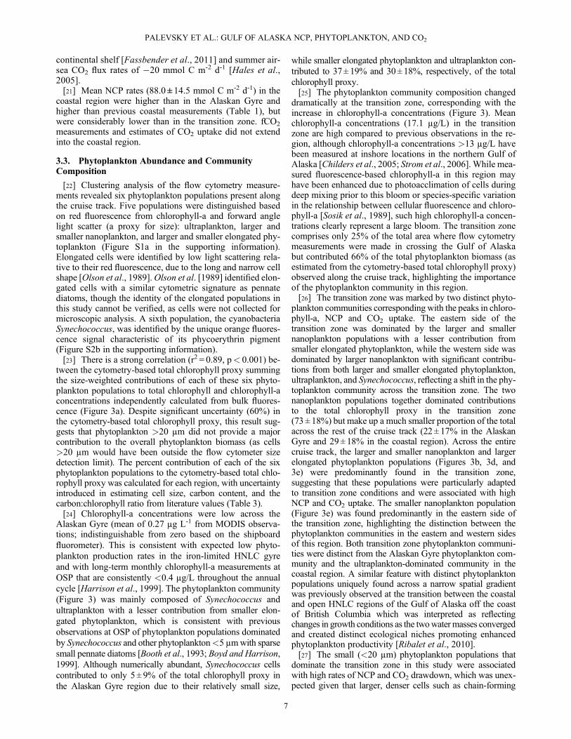
Figure 1. (a) Satellite-based surface currents and chlorophyll-a concentrations (μg/L) in the Gulf ofAlaska at the time of this study. The 2000 m isobath indicates the location of the continental slope. Thecruise track is in black, with the transition zone highlighted in gray. The transition zone is differentiatedfrom the Alaskan Gyre to the east and coastal region to the west based on elevated surface chlorophyll-aconcentrations. (b) Sea surface temperature (SST) and salinity, (c) surface nitrate and chlorophyll-a concen-trations, (d) ΔO2/Ar and ΔfCO2, (e) NCP and air-sea CO2 flux (negative values indicate oceanic uptake ofCO2) along the cruise track, calculated from ΔO2/Ar and ΔfCO2 following equations (2) and (3), respec-tively, both in units of mmol C m-2 d-1. (f) Estimated mixed layer depth (MLD) and halocline depth fromseven Argo depth profiles along the cruise track. The transition zone is highlighted in gray in all plots.


3

variability (±2σ). Combining this spread of parameterizationswith error introduced into the time-weighting by uncertaintyin MLD calculations (see section 2.5), we estimate that ourparameterization of kO2 is accurate to ±15–20% (1σ), withvariation in uncertainty across the cruise track due to windspeed variations. The uncertainty in NCP values ranges from15–55% with a median uncertainty of 20% that reflects thecombination of this location-specific uncertainty due to gas ex-change parameterization and uncertainty in ΔO2/Ar. Regionalmean data are presented with error representing a 1σ confi-dence interval in the NCP estimate rather than spatial variabil-ity across the region. To calculate NCP in carbon rather thanoxygen units, we converted using a ratio of 1 C: 1.4 O2

[Laws, 1991].

2.3. Underway Measurements of fCO2 and EstimatingAir-Sea CO2 Flux

[10] An underway IR-detection-based system (previouslydescribed in detail by Feely et al., [1998] and Pierrot et al.,[2009]) was used to make continuous measurements of sur-face ocean and atmospheric fugacity of CO2 (fCO2) accurateto ±2 μatm. Due to a shorter integration time in the CO2

equilibrator system than in the EIMS O2/Ar measurements,fCO2 is measured at a spatial resolution finer than that ofEIMS-based measurements (~1 km versus ~4 km forEIMS). The net air-sea flux of CO2 is calculated based onthe air-sea gradient in fCO2 (ΔfCO2):

Air-sea CO2flux ¼ kCO2*K0*ΔfCO2*ρ (3)

where kCO2 (m d-1) is the air-sea gas transfer velocity, calcu-lated as described above, K0 (mol kg-1 atm-1) is the tempera-ture- and salinity-dependent solubility of CO2 [Weiss, 1974],ΔfCO2 (μatm) = fCO2,ocean – fCO2,atmosphere, and ρ (kg m-3)is the seawater density. Where the air-sea CO2 flux is nega-tive, the ocean takes up CO2 from the atmosphere. The uncer-tainty in air-sea CO2 flux values ranges from 15–100%with amedian uncertainty of 29% that reflects both uncertainty inkCO2 (±15–20%, as explained above) and uncertainty inΔfCO2 measurement, with regional mean data presented witherror representing a 1σ confidence interval in the CO2 fluxestimate rather than spatial variability across the region.

2.4. Underway Flow Cytometry Measurements

[11] Continuous underway measurements of phytoplank-ton abundance and composition were made using SeaFlow,a flow-through cytometer that utilizes light scattering and cel-lular autofluorescence properties of individual cells to dis-criminate phytoplankton populations that span 1–20 μm innominal cell size [Swalwell et al., 2011]. Data files were cre-ated every 3 min, yielding a sampling resolution along thecruise track of ~1 km. Data were analyzed using the R pack-age flowPhyto [Ribalet et al., 2011], which uses statisticalclustering methods to automate the identification of phyto-plankton populations. Populations were distinguished basedon five analysis parameters: forward scatter (a proxy for cellsize) in orthogonal and perpendicular polarization states, redfluorescence from chlorophyll (collected using a 692-40band-pass filter), a second red fluorescence chlorophylldetector for large particles, and orange fluorescence fromphycoerythrin (collected using a 527-27 band-pass filter). Achange point detection algorithm developed by Aghaeepour

et al. [2011] was used to determine the optimal number ofpopulations present in each sample. When necessary, fileswere concatenated so a sufficient number of cells (at least300) were present in order to perform aggregate statisticsfor each population. To generate an estimate of the phyto-plankton biomass observed by SeaFlow, a total chlorophyllproxy that sums the size-weighted contributions of allphytoplankton populations was calculated using population-specific cell concentrations, estimates of population-specificcell size based on light scattering, size-specific cell volumeto cell carbon ratios (mean of values from Booth et al.[1988], Verity et al. [1992], and Montagnes et al. [1994]),and a carbon:chlorophyll ratio of 60:1 [Frost, 1993]. We esti-mate that this total chlorophyll proxy is accurate to ±60%, as-suming an uncertainty of ±30% in cell size estimates, ±40% incell volume to cell carbon ratios (reflecting the standard devi-ation of the three literature values for each population), and±30% in the carbon:chlorophyll ratio.

2.5. Halocline and Mixed Layer Depths (MLDs)

[12] Mixed layer and halocline depths along the cruisetrack were estimated based on depth profiles of temperatureand salinity measured on seven Argo floats during the sametime period as shipboard sampling (3–8May 2010), with sur-face-most measurements at 4 m and depth resolution of 10 mfrom 10 to 300 m. Argo profiles were taken from within 12.5km of the cruise track with the exception of a single profilerepresentative of the open Alaskan Gyre region (147.3°W)taken 75 km from the cruise track.[13] MLD was calculated based on density change from

the reference depth of 4 m. Due to thermal stratificationinduced by springtime surface warming, MLD at some loca-tions was sensitive to the selection of a density change crite-rion (Δσθ). A range of criteria have commonly been appliedboth worldwide and in the North Pacific, from 0.03 kg m-3

[De Boyer Montégut et al., 2004; Thomson and Fine, 2003]to 0.125 kg m-3 [Monterey and Levitus, 1997; Suga et al.,2004]. The intermediate criterion of Δσθ= 0.08 kg m-3 wasselected to most accurately reflect MLDs estimated by visualinspection of the individual depth profiles to account for theeffects of thermal stratification. The full range of criteria from0.03 kg m-3 to 0.125 kg m-3 was used to calculate ranges ofpotential MLDs over the period of stratification, which wereused to calculate uncertainty in the time-weighted parameter-ization of kO2. Halocline depth was calculated using salinitychange criteria (ΔS) from 4 m of 0.25.

2.6. Satellite-Based Data

[14] The following satellite-based data were used in thisstudy: 5-day averaged surface current velocity and directionfrom OSCAR (http://www.oscar.noaa.gov); dynamic seasurface height anomalies from AVISO (http://www.aviso.oceanobs.com); MODIS 8-day averaged sea surface temper-atures and chlorophyll-a concentrations and net primary pro-duction rates calculated using the vertically generalizedproduction model (VGPM) [Behrenfeld and Falkowski,1997] and the carbon-based production model (CbPM)[Westberry et al., 2008] from the Oregon State OceanProductivity site (http://www.science.oregonstate.edu/ocean.productivity); and daily wind speeds from the NOAANational Climatic Data Center (NCDC)’s multiple-satelliteBlended Sea Winds product (http://www.ncdc.noaa.gov/oa/


4

http://www.ncdc.noaa.gov/oa/rsad/air-sea/seawinds.html

rsad/air-sea/seawinds.html). The NOAA NCDC Blended SeaWinds (0.25° gridded global resolution) were validated forour study by comparison of daily satellite-based wind speedsat Ocean Station Papa (OSP, 50°N, 145°W) from the time ofthe cruise and sixty days prior with mooring-based daily-aver-aged wind speed measurements at OSP (http://www.pmel.noaa.gov/stnP) from the same time period, corrected to 10 mabove sea level, resulting in a root mean squared error of 1m s-1 with no systematic bias. This accuracy is comparableto that found in a previous comparison between NOAANCDC Blended SeaWinds and a global data set of buoy windobservations [Bentamy et al., 2009].

3. Results and Discussion

3.1. Regional Setting

[15] Circulation in the Gulf of Alaska is dominated by thecyclonic Alaskan Gyre with geostrophically driven surfacecurrents, as can be seen from satellite-derived surface currentdata from the time of the cruise (Figure 1a). The shelf regionis dominated by the Alaska Coastal Current (ACC), which isdriven west along the coastline by alongshore winds and sig-nificant freshwater runoff [Stabeno et al., 2004] and theAlaskan Stream, which flows southwest along the AlaskanPeninsula slope, offshore of the ACC, as the western bound-ary current of the Alaskan gyre [Favorite et al., 1976;Stabeno et al., 2004]. Our data show a strong salinity frontover the continental slope (Figure 1b), with low salinity in-shore of this front (west of 162.9°W) consistent with theexpected low salinity signature of the Alaskan Stream(<32.6 psu, [Favorite et al., 1976]).[16] Satellite-based chlorophyll-a concentrations indicate

that the highest phytoplankton biomass in the Gulf ofAlaska at the time of our study occurred just east of this salin-ity front, offshore of the Alaskan Peninsula slope (Figure 1a).This high-chlorophyll feature was evident from measure-ments along the cruise track, which show a region of elevatedchlorophyll-a concentrations reaching 30 μg L-1 that ex-tended from 162.9°W to 155.8°W, between the continentalslope salinity front to the west and the center of theAlaskan gyre circulation to the east (Figure 1c). This regionof elevated chlorophyll along the cruise track was markedby surface waters that were warmer and fresher than the adja-cent open Gulf of Alaska region, with decreased nitrate con-centrations and elevated O2/Ar supersaturation, fCO2

undersaturation, NCP and CO2 uptake, and shallow mixedlayers (Figures 1b–1f). For the purposes of this paper, thisregion of elevated chlorophyll-a concentration is defined asa transition zone, with the Alaskan Gyre to the southeastand the coastal region to the northwest.[17] Although this transition zone is primarily distinguished

based on high phytoplankton biomass, the distinction amongthe three regions is also supported by different nitrate-salinity(NO3-S) relationships (Figure 2). The Alaskan Gyre regionshows a consistent linear relationship between nitrate concen-trations and salinity (r2 = 0.90, p< 0.01), similar to that previ-ously described in depth profiles from straits through theAleutian Islands [Mordy et al., 2005] and the northern coastalGulf of Alaska [Childers et al., 2005; Ladd et al., 2005]. Datafrom the P17N CLIVAR line across the Gulf of Alaska(Stations 71–77: 50°N, 152°W to 55.5°N, 152.9°W; data notshown) during the end of the winter season in March 2006

showed the same linear NO3-S relationship in surface waterand in depth profiles, indicating that this relationship extendsto surface waters prior to spring biological nitrate drawdown.This suggests that the strong NO3-S relationship observed inAlaskan Gyre surface waters inMay 2010 reflects entrainmentof deep nutrient-rich, higher salinity water during the winter asthe mixed layer deepens down to the permanent halocline(Figure 1f), with little subsequent nitrate drawdown by thetime of the cruise. Water masses from the coastal region andtransition zone do not fall on this line. The coastal water is dis-tinctly fresher than the Alaskan Gyre waters but with highernitrate concentrations than would be predicted by theAlaskan Gyre NO3-S relationship, reflecting significant fresh-water input from the Alaskan Stream and ACC. The transitionzone is distinguished by nitrate concentrations that are consis-tently lower than the observed linear NO3-S relationship fromthe Alaskan Gyre for a similar range in salinity, reflecting eitherbiological nitrate drawdown or a contribution from awater masswith a different NO3-S relationship than the Alaskan Gyre.

3.2. Estimates of NCP and CO2 Flux from ΔO2/Arand ΔfCO2

[18] The trends in dissolved gas concentrations (ΔO2/Arand ΔfCO2) rather than variations in gas transfer velocitieswere the dominant terms when calculating NCP and CO2 fluxrates from equations (2) and (3), although variations in windspeed across the cruise track yielded gas transfer velocities(kO2 and kCO2) ranging from 4.5 to 9.8 m d-1 (Figures 1dand 1e). Gas residence times (i.e., mixed layer depth / gastransfer velocity) in the Alaskan Gyre ranged from 2–14 dayswhile the shallower mixed layer depths in the transition zoneand coastal region (Figure 1f) led to shorter gas residencetimes of 2–4 days. While the Alaskan Gyre region moreclosely approximates steady state conditions than the transi-tion zone and coastal regions, these short residence times

Figure 2. Sea surface nitrate concentrations plotted versussalinity for all regions along the cruise track. The linear re-gression for the Alaskan Gyre region (r2 = 0.90, p< 0.01) isshown in black.


5

http://www.ncdc.noaa.gov/oa/rsad/air-sea/seawinds.html

http://www.pmel.noaa.gov/stnP

http://www.pmel.noaa.gov/stnP

support the applicability of the steady state model used to cal-culate NCP and CO2 flux in the transition zone and coastal re-gions despite the fast current speeds (i.e., at the maximumobserved current velocity, water would only be advected~30 km during the maximal 4 day gas residence time).[19] During the time of the cruise, ΔO2/Ar in the Alaskan

Gyre was consistently supersaturated (2.2%± 0.3%), indicat-ing net autotrophic conditions with a mean NCP rate of35.1 ± 8.9 mmol C m-2 d-1. This is slightly higher than previ-ously measured values in this region, where summer NCP es-timates based on gas and nitrate budgets have ranged from 9to 27 mmol C m-2 d-1 (Table 1). Surface ocean fCO2 was un-dersaturated in the portion of the Alaskan Gyre east of thegyre center, while at the gyre center (152.2°W to 155.5°W),surface ocean fCO2 was supersaturated with respect to the at-mosphere, indicating net CO2 outgassing (mean air-sea CO2

flux of 15.7 ± 3.2 mmol C m-2 d-1) consistent with an input ofentrained deep water from winter mixing as suggested by theNO3-S relationship (Figure 2). Overall, the Alaskan Gyre re-gion was a net CO2 sink (mean air-sea CO2 flux of�5.1 ± 1.2mmol C m-2 d-1), with a slightly higher rate of CO2 uptakethan previously reported at OSP in the month of May[Wong and Chan 1991] (Table 2). This region is also a netCO2 sink on an annual basis, with estimates of air-sea CO2 fluxin the Alaskan Gyre ranging from �1.7 to 0 mol C m-2 yr-1

(Table 2). Ecosystem/carbon fluxmodel simulations comparinga biotic to an abiotic ocean at OSP indicate that biologicalproduction plays an important role in driving net carbon uptakein this region [Signorini et al., 2001].[20] The maximum ΔO2/Ar supersaturation (up to 22.7%)

and fCO2 undersaturation (fCO2 down to 196 μatm) along

the cruise track were observed in the transition zone. NCPand CO2 uptake rates varied in concert, with a high degreeof correlation (r2 = 0.73, p< 0.01) throughout the transitionzone, indicating that the CO2 uptake in this region was pri-marily driven by biological production. NCP rates were~6× higher than CO2 uptake rates, which is the result of themixed layer O2 budget being dominated by NCP and O2

gas exchange with a short air-sea equilibration time (days)whereas the mixed layer CO2 budget is dominated by NCPand physical CO2 supply with a longer air-sea equilibrationtime (months). Coincident with high chlorophyll-a concen-trations, two distinct peaks of elevated NCP and CO2 uptakewere observed in the transition zone, yielding a mean transi-tion zone NCP rate of 249 ± 40 mmol C m-2 d-1 and meantransition zone air-sea CO2 flux of �42.3±6.1 mmol C m-2 d-1.These NCP and CO2 uptake rates are large as compared tothose previously reported for the Gulf of Alaska (Tables 1and 2). Although little attention has previously been fo-cused on this transition zone region, strong negativeΔpCO2 values for the region off the Aleutian Peninsulawere measured in summer (May–August) during repeatedsurface pCO2 transects across the North Pacific, includingsurface water pCO2 as low as 150 μatm measured in May1997 [Murphy et al., 2001; Zeng et al., 2002]. Such highNCP and CO2 uptake rates have been previously observedelsewhere in ocean margin regions experiencing episodicperiods of high biological production. During the easternBering Sea spring bloom, NCP can reach rates of360–1300 mmol C m-2 d-1 [Prokopenko et al., 2010], whileeastern north Pacific coastal upwelling systems can produceNCP rates of up to 1200 ± 420 mmol C m-2 d-1on the

Table 1. Summary of NCP Rates From Open Ocean and Coastal Studies in the Gulf of Alaska

May Annual

Source(mmol C m-2 d-1) (mol C m-2 yr-1)

Alaskan Gyre 17a 2.5 Emerson and Stump [2010]9–12a (1.6)b Emerson et al. [1991]15a (2.1 ± 1.5)b Emerson [1987]7.1 Charette et al. [1999]26.6a Wheeler [1993] (NO3 budget)

21.3 ± 2.2a Wheeler [1993] (15N incubations)(20.3)a,b 3.05 Wong et al. [2002]35.1 ± 8.9 This study

Transition zone and coastal region 3.89 Wong et al. [2002]249 ± 40 (transition)88.0 ± 14.5 (coastal)

This study

aWhole-summer rather than May values.bParentheses denote values calculated based on Emerson and Stump's [2010] conclusion (based on year-round data from a mooring at OSP) that summer

production occurring over 150 days drives essentially all annual biological carbon export, with little or no net export production in winter.

Table 2. Summary of Air-Sea CO2 Flux Rates From Open Ocean and Coastal Studies in the Gulf of Alaska

May Annual

Source(mmol C m-2 d-1) (mol C m-2 yr-1)

Alaskan Gyre �3.5, –4.4 �0.7 Wong and Chan [1991]�0.6 Chierici et al. [2006]

�1.7–0 Takahashi et al. [2009]�5.1 ± 1.2 This study

Transition zone and coastal region �27.6 ± 6.7a Ribalet et al. [2010]�1.8 Chen and Borges [2009]

�42.3 ± 6.1 This study

aJune rather than May values.


6

continental shelf [Fassbender et al., 2011] and summer air-sea CO2 flux rates of �20 mmol C m-2 d-1 [Hales et al.,2005].[21] Mean NCP rates (88.0 ± 14.5 mmol C m-2 d-1) in the

coastal region were higher than in the Alaskan Gyre andhigher than previous coastal measurements (Table 1), butwere considerably lower than in the transition zone. fCO2

measurements and estimates of CO2 uptake did not extendinto the coastal region.

3.3. Phytoplankton Abundance and CommunityComposition

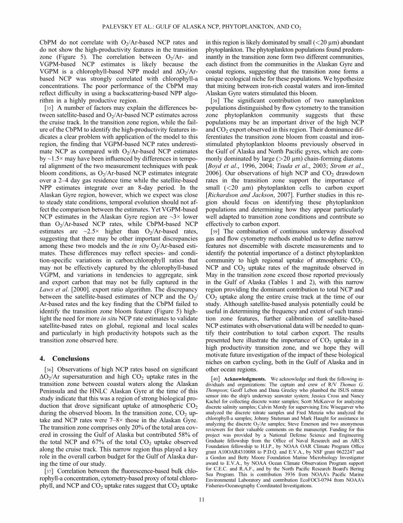
[22] Clustering analysis of the flow cytometry measure-ments revealed six phytoplankton populations present alongthe cruise track. Five populations were distinguished basedon red fluorescence from chlorophyll-a and forward anglelight scatter (a proxy for size): ultraplankton, larger andsmaller nanoplankton, and larger and smaller elongated phy-toplankton (Figure S1a in the supporting information).Elongated cells were identified by low light scattering rela-tive to their red fluorescence, due to the long and narrow cellshape [Olson et al., 1989].Olson et al. [1989] identified elon-gated cells with a similar cytometric signature as pennatediatoms, though the identity of the elongated populations inthis study cannot be verified, as cells were not collected formicroscopic analysis. A sixth population, the cyanobacteriaSynechococcus, was identified by the unique orange fluores-cence signal characteristic of its phycoerythrin pigment(Figure S2b in the supporting information).[23] There is a strong correlation (r2 = 0.89, p< 0.001) be-

tween the cytometry-based total chlorophyll proxy summingthe size-weighted contributions of each of these six phyto-plankton populations to total chlorophyll and chlorophyll-aconcentrations independently calculated from bulk fluores-cence (Figure 3a). Despite significant uncertainty (60%) inthe cytometry-based total chlorophyll proxy, this result sug-gests that phytoplankton >20 μm did not provide a majorcontribution to the overall phytoplankton biomass (as cells>20 μm would have been outside the flow cytometer sizedetection limit). The percent contribution of each of the sixphytoplankton populations to the cytometry-based total chlo-rophyll proxy was calculated for each region, with uncertaintyintroduced in estimating cell size, carbon content, and thecarbon:chlorophyll ratio from literature values (Table 3).[24] Chlorophyll-a concentrations were low across the

Alaskan Gyre (mean of 0.27 μg L-1 from MODIS observa-tions; indistinguishable from zero based on the shipboardfluorometer). This is consistent with expected low phyto-plankton production rates in the iron-limited HNLC gyreand with long-term monthly chlorophyll-a measurements atOSP that are consistently <0.4 μg/L throughout the annualcycle [Harrison et al., 1999]. The phytoplankton community(Figure 3) was mainly composed of Synechococcus andultraplankton with a lesser contribution from smaller elon-gated phytoplankton, which is consistent with previousobservations at OSP of phytoplankton populations dominatedby Synechococcus and other phytoplankton<5 μmwith sparsesmall pennate diatoms [Booth et al., 1993; Boyd and Harrison,1999]. Although numerically abundant, Synechococcus cellscontributed to only 5 ± 9% of the total chlorophyll proxy inthe Alaskan Gyre region due to their relatively small size,

while smaller elongated phytoplankton and ultraplankton con-tributed to 37± 19% and 30±18%, respectively, of the totalchlorophyll proxy.[25] The phytoplankton community composition changed

dramatically at the transition zone, corresponding with theincrease in chlorophyll-a concentrations (Figure 3). Meanchlorophyll-a concentrations (17.1 μg/L) in the transitionzone are high compared to previous observations in the re-gion, although chlorophyll-a concentrations >13 μg/L havebeen measured at inshore locations in the northern Gulf ofAlaska [Childers et al., 2005; Strom et al., 2006]. While mea-sured fluorescence-based chlorophyll-a in this region mayhave been enhanced due to photoacclimation of cells duringdeep mixing prior to this bloom or species-specific variationin the relationship between cellular fluorescence and chloro-phyll-a [Sosik et al., 1989], such high chlorophyll-a concen-trations clearly represent a large bloom. The transition zonecomprises only 25% of the total area where flow cytometrymeasurements were made in crossing the Gulf of Alaskabut contributed 66% of the total phytoplankton biomass (asestimated from the cytometry-based total chlorophyll proxy)observed along the cruise track, highlighting the importanceof the phytoplankton community in this region.[26] The transition zone was marked by two distinct phyto-

plankton communities corresponding with the peaks in chloro-phyll-a, NCP and CO2 uptake. The eastern side of thetransition zone was dominated by the larger and smallernanoplankton populations with a lesser contribution fromsmaller elongated phytoplankton, while the western side wasdominated by larger nanoplankton with significant contribu-tions from both larger and smaller elongated phytoplankton,ultraplankton, and Synechococcus, reflecting a shift in the phy-toplankton community across the transition zone. The twonanoplankton populations together dominated contributionsto the total chlorophyll proxy in the transition zone(73 ± 18%) but make up a much smaller proportion of the totalacross the rest of the cruise track (22 ± 17% in the AlaskanGyre and 29± 18% in the coastal region). Across the entirecruise track, the larger and smaller nanoplankton and largerelongated phytoplankton populations (Figures 3b, 3d, and3e) were predominantly found in the transition zone,suggesting that these populations were particularly adaptedto transition zone conditions and were associated with highNCP and CO2 uptake. The smaller nanoplankton population(Figure 3e) was found predominantly in the eastern side ofthe transition zone, highlighting the distinction between thephytoplankton communities in the eastern and western sidesof this region. Both transition zone phytoplankton communi-ties were distinct from the Alaskan Gyre phytoplankton com-munity and the ultraplankton-dominated community in thecoastal region. A similar feature with distinct phytoplanktonpopulations uniquely found across a narrow spatial gradientwas previously observed at the transition between the coastaland open HNLC regions of the Gulf of Alaska off the coastof British Columbia which was interpreted as reflectingchanges in growth conditions as the twowatermasses convergedand created distinct ecological niches promoting enhancedphytoplankton productivity [Ribalet et al., 2010].[27] The small (<20 μm) phytoplankton populations that

dominate the transition zone in this study were associatedwith high rates of NCP and CO2 drawdown, which was unex-pected given that larger, denser cells such as chain-forming


7

Figure 3. (a) Chlorophyll-a concentrations along the cruise track from fluorometry-based measurementsand a cytometry-based proxy for total chlorophyll calculated based on estimates of cell-specific chlorophyllcontent for each phytoplankton population shown below. (b–g) Cell abundance along the cruise track forsix phytoplankton populations identified by underway flow cytometry (see text and Figure S1 in thesupporting information for description of clustering methods used to distinguish populations).Populations are ordered by nominal cell size from (Figure 3b) largest to (Figure 3g) smallest. The transitionzone is highlighted in gray. The transition zone is differentiated from the Alaskan Gyre to the east andcoastal region to the west based on elevated surface chlorophyll-a concentrations.


8

diatoms are thought to lead to more efficient and higher ratesof carbon export [Smayda, 1970; Boyd and Newton, 1995,1999]. Previous studies have suggested that aggregation ofcells and packaging by grazers can allow small cells to contrib-ute more efficiently to carbon export [Francois et al., 2002;Lutz et al., 2007; Richardson and Jackson, 2007; Kahl et al.,2008; Stukel et al., 2011]. Further study will be necessary toevaluate the role of these mechanisms in the transition zonephytoplankton communities observed here.

3.4. Explaining Enhanced Biological Productivityin the Transition Zone

[28] A number of previous studies have suggested thatincreased iron availability at the convergence between iron-limited HNLC waters and iron-rich coastal waters in theGulf of Alaska could stimulate phytoplankton production[e.g., Whitney et al., 2005; Strom et al., 2006; Ribalet et al.,2010]. Glacial meltwater input along the coast provides asource of particulate and dissolved iron to the ACC, whichmixes with low-iron offshore waters to create a cross-shelf gra-dient in iron availability [Wu et al., 2009; Lippiatt et al., 2010].Recirculation of flow from the Alaskan Stream into theAlaskan Gyre can transport iron-rich coastal waters offshoreand stimulate phytoplankton production [Favorite et al.,1976; Whitney et al., 2005]. Mesoscale anticyclonic eddies,which propagate along the Alaskan Peninsula, can also supplycoastally derived iron to offshore iron-limited waters [Johnsonet al., 2005; Lippiatt et al., 2011; Peterson et al., 2011].However, analysis of dynamic sea surface height anomalies(AVISO) does not provide evidence of eddies in the vicinityof the transition zone at the time of our cruise.[29] Surface water properties along the cruise track show a

distinct separation between the Alaskan Gyre and the coastalregions, with the coastal region particularly marked by a dis-tinct freshwater signature (Figure 1b and Figure S2 in thesupporting information). While there is a potential role formixing between these water masses in the transition zone, thisrelationship is complex, as the Alaskan Stream suppliescoastal water carried alongshore from the northeast, whichmay not match the properties of the coastal waters sampledalong our cruise track. Mixing within the transition zone is het-erogeneous, with two regions of pronounced warming andfreshening corresponding with elevated chlorophyll-a concen-trations (Figures 1b and 1c) and freshening correlated with in-creased NCP rates in the region east of the salinity front(Figure 4b; r2 = 0.62, p< 0.01), suggesting that input of freshcoastal water contributed to elevated biological production.[30] We therefore hypothesize that the high phytoplankton

abundance and NCP rates in the transition region were fueled

by coastal iron input to iron-limited Alaskan Gyre HNLCwaters. Although iron concentrations were not measured dur-ing the cruise, this hypothesis is supported by previous mea-surements of total dissolved iron concentrations along theAlaskan Peninsula slope near the region of the transitionzone, which were ~50-fold higher than at OSP, andcorresponded with an increase in phytoplankton photosyn-thetic efficiency (Fv/Fm) as compared to the Alaskan Gyre[Suzuki et al., 2002]. It is also supported by the presence ofthe larger elongated phytoplankton population predomi-nantly found in the transition zone (Figure 3b), which al-though only a minor contribution to the overall transitionzone phytoplankton community (12 ± 14%), likely representspennate diatoms such as Pseudo-nitszchia that have beenshown to respond to addition of iron [Marchetti et al., 2006].[31] It is noteworthy that while spring blooms do occur

across the coastal region in the Gulf of Alaska, it is highly un-usual for them to be as large as the transition zone bloom weobserved. The coastal region of our study exhibited NCPrates and chlorophyll-a concentrations lower than those ob-served in the transition zone, though higher than those inthe Alaskan Gyre. The coastal chlorophyll-a concentrationswere within the range of previous observations of the Mayspring bloom period in the northern coastal Gulf of Alaska

32.5 33 33.50

100

200

300

400

Salinity (psu)

NC

P (

mm

ol C

m−

2 d−

1 )

Figure 4. Transition zone NCP rates plotted versus salinity,with the linear regression (r2 = 0.62, p< 0.01) shown in black.

Table 3. Proportional Contribution of Phytoplankton Populations to Total Chlorophyll (proxy) by Regiona

Larger ElongatedPhytoplankton

Smaller ElongatedPhytoplankton

LargerNanoplankton

SmallerNanoplankton Ultraplankton Synechococcus

Mean Chlorophyll-a(μg/L)

AlaskanGyre

6 ± 10% 37± 19% 6± 10% 16± 15% 30± 18% 5± 9% 0.27b

Transitionzone

12 ± 14% 8± 12% 48± 20% 25± 17% 6± 10% 1± 4% 17.1

Coastalregion

2 ± 7% 19± 16% 18± 16% 11± 13% 49± 20% 2± 7% 0.96

aUncertainty in proportional contributions is calculated based on propagation of 60% uncertainty in the total chlorophyll proxy.bBased on MODIS satellite observations, as chlorophyll-a estimates from the shipboard fluorometer were indistinguishable from zero.


9

[Strom et al., 2006]. Onset of the spring phytoplanktonbloom in the nutrient-replete inshore coastal Gulf of Alaskais triggered by relief of wintertime light limitation, withspringtime cloud cover, extent of stratification and grazingpressure all influencing the timing and magnitude of theseblooms [Napp et al., 1996; Stabeno et al., 2004]. Light avail-ability could have limited phytoplankton production in thecoastal region at the time of our study, although shoaling ofmixed layers in response to spring thermal stratification ob-served from Argo floats in the transition zone may also haveextended to the coastal region (where Argo floats were ab-sent), which would have relieved light limitation and stimu-lated phytoplankton growth in both regions. Grazingpressure may also have reduced the size of the bloom in thecoastal region if zooplankton growth kept pace with gradu-ally increasing light availability and phytoplankton growthduring spring. The transition zone, by contrast, was likelyable to outstrip grazing pressure due to rapid phytoplanktonresponse to addition of iron.[32] The temporal evolution of the transition zone feature

is an additional important consideration. Given the meanNCP rate of 249 mmol C m-2 d-1 calculated for the transitionzone and assuming a starting nitrate concentration of themaximum observed along the cruise track (26 μM) and ni-trate consumption at a rate of 106 C: 16 N [Redfield et al.,1963], biological drawdown would consume all the availablenitrate in 12 days, suggesting that we sampled the transitionzone in the midst of a short-lived bloom. Analysis of satel-lite-based surface chlorophyll data over the two-week inter-vals prior to and following our study indicate that highestchlorophyll concentrations and largest spatial extent of thebloom occurred during the 8-day interval spanning our 5-day cruise. This temporal evolution implies that the omissionof a time rate of change term in the calculation of NCP andCO2 flux rates in equations (2) and (3), which was based onthe assumption of a steady state condition, potentiallyoverestimated NCP rates. Without the inclusion of a time rateof change term, the biomass of organic carbon in the surfacemixed layer that accumulated during the bloom (as indicatedby satellite observations of increasing chlorophyll-a concen-trations) was assumed to have been exported. However, it ispossible that some of this carbon was later remineralized dur-ing the declining phase of this bloom rather than sinking outof the mixed layer and leading to export. Thus, the transition

zone NCP estimates presented here are an upper limit on theamount of net carbon exported by the observed phytoplank-ton bloom. The observed shift in phytoplankton communitystructure across the transition zone may reflect the temporalevolution of the bloom as it spread across the transition zoneregion, with the two different phytoplankton communities inthe eastern and western side of the region reflecting early andlate stages of the bloom, as was suggested for the transitionzone phytoplankton bloom described by Ribalet et al.[2010] in the northeast Pacific. Further study in this regionwill be necessary to determine the reasons for the distinctphytoplankton community compositions and the fate of or-ganic carbon produced during short-lived transition zonebloom features.

3.5. Comparison with Satellite-BasedProduction Estimates

[33] This study presents a snapshot of conditions along ourcruise track in the Gulf of Alaska in May 2010. Satellite ob-servations provide a potentially powerful tool to extend thisanalysis to a broader spatial and temporal scale. Carbonexport rates comparable to O2/Ar-based estimates of NCPcan be calculated from satellite-based estimates of netprimary productivity (NPP), which is defined as gross photo-synthetic production minus autotrophic respiration, multi-plied by an estimate of the fraction of primary productionexported from the surface ocean. Satellite-based models havepreviously applied this approach to calculate carbon exportover the global ocean [Muller-Karger et al., 2005; Dunneet al., 2007], but there is relatively little observational dataavailable to validate this approach.[34] We compared our O2/Ar-based NCP estimates with

NCP rates calculated from satellite observations along thecruise track at the time of our study (integrated over 1–8May 2010). We used publicly available NPP data calculatedfrom the vertically generalized production model (VGPM)[Behrenfeld and Falkowski, 1997] or the carbon-basedproduction model (CbPM), [Westberry et al., 2008]. Thefraction of primary production exported from the surfaceocean was calculated using the temperature- and NPP-based export ratio algorithm of Laws et al. [2000].Satellite-based NCP rates calculated using the VGPMare correlated with O2/Ar-based NCP rates from this study(r =0.67, p <0.001), while NCP rates calculated using the

Figure 5. NCP rates calculated based on ΔO2/Ar measured in this study plotted along with NCP ratescalculated based on MODIS satellite data using the VGPM [Behrenfeld and Falkowski, 1997] andCbPM [Westberry et al., 2008] net primary production algorithms, each in combination with the exportratio algorithm of Laws et al. [2000]. The transition zone is highlighted in gray.


10

CbPM do not correlate with O2/Ar-based NCP rates anddo not show the high-productivity features in the transitionzone (Figure 5). The correlation between O2/Ar- andVGPM-based NCP estimates is likely because theVGPM is a chlorophyll-based NPP model and ΔO2/Ar-based NCP was strongly correlated with chlorophyll-aconcentrations. The poor performance of the CbPM mayreflect difficulty in using a backscattering-based NPP algo-rithm in a highly productive region.[35] A number of factors may explain the differences be-

tween satellite-based and O2/Ar-based NCP estimates acrossthe cruise track. In the transition zone region, while the fail-ure of the CbPM to identify the high-productivity features in-dicates a clear problem with application of the model to thisregion, the finding that VGPM-based NCP rates underesti-mate NCP as compared with O2/Ar-based NCP estimatesby ~1.5× may have been influenced by differences in tempo-ral alignment of the two measurement techniques with peakbloom conditions, as O2/Ar-based NCP estimates integrateover a 2–4 day gas residence time while the satellite-basedNPP estimates integrate over an 8-day period. In theAlaskan Gyre region, however, which we expect was closeto steady state conditions, temporal evolution should not af-fect the comparison between the estimates. Yet VGPM-basedNCP estimates in the Alaskan Gyre region are ~3× lowerthan O2/Ar-based NCP rates, while CbPM-based NCPestimates are ~2.5× higher than O2/Ar-based rates,suggesting that there may be other important discrepanciesamong these two models and the in situ O2/Ar-based esti-mates. These differences may reflect species- and condi-tion-specific variations in carbon:chlorophyll ratios thatmay not be effectively captured by the chlorophyll-basedVGPM, and variations in tendencies to aggregate, sinkand export carbon that may not be fully captured in theLaws et al. [2000]. export ratio algorithm. The discrepancybetween the satellite-based estimates of NCP and the O2/Ar-based rates and the key finding that the CbPM failed toidentify the transition zone bloom feature (Figure 5) high-light the need for more in situ NCP rate estimates to validatesatellite-based rates on global, regional and local scalesand particularly in high productivity hotspots such as thetransition zone observed here.

4. Conclusions

[36] Observations of high NCP rates based on significantΔO2/Ar supersaturation and high CO2 uptake rates in thetransition zone between coastal waters along the AlaskanPeninsula and the HNLC Alaskan Gyre at the time of thisstudy indicate that this was a region of strong biological pro-duction that drove significant uptake of atmospheric CO2

during the observed bloom. In the transition zone, CO2 up-take and NCP rates were 7–8× those in the Alaskan Gyre.The transition zone comprises only 20% of the total area cov-ered in crossing the Gulf of Alaska but contributed 58% ofthe total NCP and 67% of the total CO2 uptake observedalong the cruise track. This narrow region thus played a keyrole in the overall carbon budget for the Gulf of Alaska dur-ing the time of our study.[37] Correlation between the fluorescence-based bulk chlo-

rophyll-a concentration, cytometry-based proxy of total chloro-phyll, and NCP and CO2 uptake rates suggest that CO2 uptake

in this region is likely dominated by small (<20 μm) abundantphytoplankton. The phytoplankton populations found predom-inantly in the transition zone form two different communities,each distinct from the communities in the Alaskan Gyre andcoastal regions, suggesting that the transition zone forms aunique ecological niche for these populations. We hypothesizethat mixing between iron-rich coastal waters and iron-limitedAlaskan Gyre waters stimulated this bloom.[38] The significant contribution of two nanoplankton

populations distinguished by flow cytometry to the transitionzone phytoplankton community suggests that thesepopulations may be an important driver of the high NCPand CO2 export observed in this region. Their dominance dif-ferentiates the transition zone bloom from coastal and iron-stimulated phytoplankton blooms previously observed inthe Gulf of Alaska and North Pacific gyres, which are com-monly dominated by large (>20 μm) chain-forming diatoms[Boyd et al., 1996, 2004; Tsuda et al., 2003; Strom et al.,2006]. Our observations of high NCP and CO2 drawdownrates in the transition zone support the importance ofsmall (<20 μm) phytoplankton cells to carbon export[Richardson and Jackson, 2007]. Further studies in this re-gion should focus on identifying these phytoplanktonpopulations and determining how they appear particularlywell adapted to transition zone conditions and contribute soeffectively to carbon export.[39] The combination of continuous underway dissolved

gas and flow cytometry methods enabled us to define narrowfeatures not discernible with discrete measurements and toidentify the potential importance of a distinct phytoplanktoncommunity to high regional uptake of atmospheric CO2.NCP and CO2 uptake rates of the magnitude observed inMay in the transition zone exceed those reported previouslyin the Gulf of Alaska (Tables 1 and 2), with this narrowregion providing the dominant contribution to total NCP andCO2 uptake along the entire cruise track at the time of ourstudy. Although satellite-based analysis potentially could beuseful in determining the frequency and extent of such transi-tion zone features, further calibration of satellite-basedNCP estimates with observational data will be needed to quan-tify their contribution to total carbon export. The resultspresented here illustrate the importance of CO2 uptake in ahigh productivity transition zone, and we hope they willmotivate future investigation of the impact of these biologicalniches on carbon cycling, both in the Gulf of Alaska and inother ocean regions.

[40] Acknowledgments. We acknowledge and thank the following in-dividuals and organizations: The captain and crew of R/V Thomas G.Thompson; Geoff Lebon and Dana Greeley who plumbed the ISUS nitratesensor into the ship's underway seawater system; Jessica Cross and NancyKachel for collecting discrete water samples; Scott McKeever for analyzingdiscrete salinity samples; Calvin Mordy for supervising Eric Wisegarver whoanalyzed the discrete nitrate samples and Fred Menzia who analyzed thechlorophyll-a samples; Johnny Stutsman and Mark Haught for assistance inanalyzing the discrete O2/Ar samples; Steve Emerson and two anonymousreviewers for their valuable comments on the manuscript. Funding for thisproject was provided by a National Defense Science and EngineeringGraduate fellowship from the Office of Naval Research and an ARCSFoundation fellowship to H.I.P., by NOAA OAR Climate Program Officegrant A10OAR4310088 to P.D.Q. and E.V.A., by NSF grant 0622247 anda Gordon and Betty Moore Foundation Marine Microbiology Investigatoraward to E.V.A., by NOAA Ocean Climate Observation Program supportfor C.E.C. and R.A.F., and by the North Pacific Research Board's BeringSea Program. This is contribution 3936 from NOAA's Pacific MarineEnvironmental Laboratory and contribution EcoFOCI-0794 from NOAA'sFisheries-Oceanography Coordinated Investigations.


11

References

Aghaeepour, N., R. Nikolic, H. H. Hoos, and R. R. Brinkman (2011), Rapidcell population identification in flow cytometry data, Cytometry A, 79(1),6–13, doi:10.1002/cyto.a.21007.

Armstrong, F. A. J., C. R. Stearns, and J. D. H. Strickland (1967), The mea-surement of upwelling and subsequent biological processes by means ofthe Technicon AutoAnalyzer and associated equipment, Deep-Sea Res.,14, 381–389.

Behrenfeld,M. J., and P. G. Falkowski (1997), Photosynthetic rates derived fromsatellite-based chlorophyll concentration, Limnol. Oceanogr., 42(1), 1–20.

Bentamy, A., C. Croize-Fillon, P. Queffeulou, C. Liu, and H. Roquet (2009),Evaluation of high-resolution surface wind products at global and regionalscales, J. Oper. Ocean., 2(2), 15–27.

Booth, B., J. Lewin, and C. J. Lorenzen (1988), Summer growth rates of sub-arctic Pacific phytoplankton assemblages determined from carbon uptakeand cell volumes estimated using epifluorescence microscopy, Mar.Biol., 98, 287–298.

Booth, B. C., J. Lewin, and J. R. Postel (1993), Temporal variation in thestructure of autotrophic and heterotrophic communities in the subarcticPacific, Prog. Oceanogr., 32(1–4), 57–99.

Boyd, P., and P. J. Harrison (1999), Phytoplankton dynamics in the NE sub-arctic Pacific, Deep Sea Res. Part II, 46(11–12), 2405–2432, doi:10.1016/S0967-0645(99)00069-7.

Boyd, P., and P. Newton (1995), Evidence of the potential influence ofplanktonic community structure on the interannual variability of particu-late organic carbon flux, Deep Sea Res. Part I, 42(5), 619–639,doi:10.1016/0967-0637(95)00017-Z.

Boyd, P. W., and P. P. Newton (1999), Does planktonic community structuredetermine downward particulate organic carbon flux in different oceanicprovinces?, Deep Sea Res. Part I, 46(1), 63–91, doi:10.1016/S0967-0637(98)00066-1.

Boyd, P., D. Muggli, D. Varela, R. Goldblatt, R. Chretien, K. Orians, andP. Harrison (1996), In vitro iron enrichment experiments in the NE subarc-tic Pacific, Mar. Ecol. Prog. Ser., 136, 179–193.

Boyd, P. W., et al. (2004), The decline and fate of an iron-induced subarcticphytoplankton bloom,Nature, 428(6982), 549–53, doi:10.1038/nature02437.

Cassar, N., B. A. Barnett, M. L. Bender, J. Kaiser, R. C. Hamme, andB. Tilbrook (2009), Continuous high-frequency dissolved O2/Ar measure-ments by equilibrator inlet mass spectrometry, Anal. Chem., 81(5),1855–64, doi:10.1021/ac802300u.

Charette, M. A., S. B. Moran, and J. K. B. Bishop (1999), 234Th as a tracer ofparticulate organic carbon export in the subarctic northeast Pacific Ocean,Deep Sea Res. Part II, 46(11–12), 2833–2861, doi:10.1016/S0967-0645(99)00085-5.

Chen, C., and A. V. Borges (2009), Reconciling opposing views on carbon cy-cling in the coastal ocean: Continental shelves as sinks and near-shore ecosys-tems as sources of atmospheric CO2, Deep Sea Res. Part II, 56, 578–590.

Chierici, M., A. Fransson, and Y. Nojiri (2006), Biogeochemical processesas drivers of surface fCO2 in contrasting provinces in the subarctic NorthPacific Ocean, Global Biogeochem. Cycles, 20(1), 1–16, doi:10.1029/2004GB002356.

Childers, A., T. Whitledge, and D. Stockwell (2005), Seasonal andinterannual variability in the distribution of nutrients and chlorophyll aacross the Gulf of Alaska shelf: 1998–2000, Deep Sea Res. Part II,52(1–2), 193–216, doi:10.1016/j.dsr2.2004.09.018.

Craig, H., and T. Hayward (1987), Oxygen supersaturation in the ocean:Biological versus physical contributions, Science, 235(4785), 199–202.

Cunningham, A., D. McKee, S. Craig, G. Tarran, and C. Widdicombe (2003),Fine-scale variability in phytoplankton community structure and inherentoptical properties measured from an autonomous underwater vehicle,J. Mar. Syst., 43(1–2), 51–59, doi:10.1016/S0924-7963(03)00088-5.

De Boyer Montégut, C., G. Madec, A. S. Fischer, A. Lazar, and D. Iudicone(2004), Mixed layer depth over the global ocean: An examination of pro-file data and a profile-based climatology, J. Geophys. Res., 109, C12003,doi:10.1029/2004JC002378.

Dunne, J. P., J. L. Sarmiento, and A. Gnanadesikan (2007), A synthesis ofglobal particle export from the surface ocean and cycling through theocean interior and on the seafloor, Global Biogeochem. Cycles, 21(4),1–16, doi:10.1029/2006GB002907.

Emerson, S. (1987), Seasonal oxygen cycles and biological new productionin surface waters of the subarctic Pacific Ocean, J. Geophys. Res., 92(C6),6535–6544.

Emerson, S., and C. Stump (2010), Net biological oxygen production in theocean—II: Remote in situ measurements of O2 and N2 in subarctic pacificsurface waters, Deep Sea Res. Part I, 57(10), 1255–1265, doi:10.1016/j.dsr.2010.06.001.

Emerson, S., P. Quay, C. Stump, D. Wilbur, andM. Knox (1991), O2, Ar, N2and 222Rn in surface waters of the subarctic ocean: net biological O2 pro-duction, Global Biogeochem. Cycles, 5(1), 49–69.

Emerson, S., P. D. Quay, C. Stump, D. Wilbur, and R. Schudlich (1995),Chemical tracers of productivity and respiration in the subtropical PacificOcean, J. Geophys. Res., 100(C8), 15873–15887, doi:10.1029/95JC01333.

Fassbender, A. J., C. L. Sabine, R. A. Feely, C. Langdon, and C. W. Mordy(2011), Inorganic carbon dynamics during northern California coastal upwell-ing, Cont. Shelf Res., 31(11), 1180–1192, doi:10.1016/j.csr.2011.04.006.

Favorite, F., A. J. Dodimead, and K. Nasu (1976), Oceanography of theSubarctic Pacific Region, 1960–1971, Bulletin No. 33, 187 pp.,International North Pacific Fisheries Commission, Vancouver, Canada.

Feely, R. A., R. Wanninkhof, H. B. Milburn, C. E. Cosca, and M. Stapp(1998), A new automated underway system for making high precisionpCO2 measurements onboard research ships, Anal. Chim. Acta,377(2–3), 185–191.

Francois, R., S. Honjo, R. Krishfield, and S. Manganini (2002), Factors con-trolling the flux of organic carbon to the bathypelagic zone of the ocean,Global Biogeochem. Cycles, 16(4), doi:10.1029/2001GB001722.

Friedlingstein, P., R. A. Houghton, G. Marland, J. Hackler, T. A. Boden,T. J. Conway, J. G. Canadell, M. R. Raupach, P. Ciais, and C. Le Quéré(2010), Update on CO2 emissions, Nature Geosci., 3(12), 811–812,doi:10.1038/ngeo1022.

Frost, B. W. (1993), A modelling study of processes regulating planktonstanding stock and production in the open subarctic Pacific Ocean, Prog.Oceanogr., 32(1–4), 17–56, doi:10.1016/0079-6611(93)90008-2.

Garcia, H. E., and L. I. Gordon (1992), Oxygen solubility in seawater: Betterfitting solubility equations, Limnol. Oceanogr., 37(6), 1307–1312.

Hales, B., T. Takahashi, and L. Bandstra (2005), Atmospheric CO2 uptakeby a coastal upwelling system, Global Biogeochem. Cycles, 19(1), 1–11,doi:10.1029/2004GB002295.

Hamme, R., and S. Emerson (2004), The solubility of neon, nitrogen andargon in distilled water and seawater, Deep Sea Res. Part I, 51(11),1517–1528, doi:10.1016/j.dsr.2004.06.009.

Harrison, P., P. Boyd, D. Varela, S. Takeda, A. Shiomoto, and T. Odate (1999),Comparison of factors controlling phytoplankton productivity in the NE andNW subarctic Pacific gyres, Prog. Oceanogr., 43(2–4), 205–234.

Ho, D. T., C. S. Law, M. J. Smith, P. Schlosser, M. Harvey, and P. Hill(2006), Measurements of air-sea gas exchange at high wind speeds inthe Southern Ocean: Implications for global parameterizations, Geophys.Res. Lett., 33, L16611, doi:10.1029/2006GL026817.

Johnson, W. K., L. A. Miller, N. E. Sutherland, and C. S. Wong (2005), Irontransport by mesoscale Haida eddies in the Gulf of Alaska, Deep Sea Res.Part II, 52(7–8), 933–953, doi:10.1016/j.dsr2.2004.08.017.

Juranek, L. W., and P. D. Quay (2005), In vitro and in situ gross primary andnet community production in the North Pacific Subtropical Gyre using la-beled and natural abundance isotopes of dissolved O2, GlobalBiogeochem. Cycles, 19(3), doi:10.1029/2004GB002384.

Kahl, L., A. Vardi, and O. Schofield (2008), Effects of phytoplankton phys-iology on export flux, Mar. Ecol. Prog. Ser., 354, 3–19, doi:10.3354/meps07333.

Ladd, C., N. B. Kachel, C. W. Mordy, and P. J. Stabeno (2005),Observations from a Yakutat eddy in the northern Gulf of Alaska,J. Geophys. Res., 110, C03003, doi:10.1029/2004JC002710.

Laws, E. A. (1991), Photosynthetic quotients, new production and net com-munity production in the open ocean, Deep-Sea Res., 38(1), 143–167.

Laws, E., P. Falkowski, W. J. Smith, H. Ducklow, and J. McCarthy (2000),Temperature effects on export production in the open ocean, GlobalBiogeochem. Cycles, 14(4), 1231–1246.

Le Quéré, C., et al. (2009), Trends in the sources and sinks of carbon dioxide,Nature Geosci., 2(12), 831–836, doi:10.1038/ngeo689.

Lippiatt, S. M., M. C. Lohan, and K. W. Bruland (2010), The distribution ofreactive iron in northern Gulf of Alaska coastal waters, Mar. Chem.,121(1–4), 187–199, doi:10.1016/j.marchem.2010.04.007.

Lippiatt, S. M., M. T. Brown, M. C. Lohan, and K. W. Bruland (2011),Reactive iron delivery to the Gulf of Alaska via a Kenai eddy, Deep SeaRes. Part I, 58(11), 1091–1102, doi:10.1016/j.dsr.2011.08.005.

Liss, P. S., and L. Merlivat (1986), Air-sea gas exchange rates: Introductionand synthesis, in The Role of Air-Sea Exchange in Geochemical Cycling,edited by P. Buat-Menard, pp. 113–129, D. Reidel, Hingham, Mass.

Lorenzen, C. J. (1966), A method for the continuous measurement of in vivochlorophyll concentration, in Deep Sea Res., vol. 13, pp. 223–227, Elsevier.

Lutz, M. J., K. Caldeira, R. B. Dunbar, and M. J. Behrenfeld (2007),Seasonal rhythms of net primary production and particulate organic carbonflux to depth describe the efficiency of biological pump in the globalocean, J. Geophys. Res., 112, C10011, doi:10.1029/2006JC003706.

Marchetti, A., N. D. Sherry, H. Kiyosawa, A. Tsuda, and P. J. Harrison(2006), Phytoplankton processes during a mesoscale iron enrichment inthe NE subarctic Pacific: Part I—Biomass and assemblage, Deep SeaRes. Part II, 53(20–22), 2095–2113, doi:10.1016/j.dsr2.2006.05.038.

Marinov, I., M. Follows, A. Gnanadesikan, J. L. Sarmiento, and R. D. Slater(2008), How does ocean biology affect atmospheric pCO2? Theory andmodels, J. Geophys. Res., 113, C07032, doi:10.1029/2007JC004598.


12

Martin, J. H., and S. E. Fitzwater (1988), Iron deficiency limits phytoplank-ton growth in the north-east Pacific subarctic, Nature, 331, 341–343.

Montagnes, D. J. S., J. A. Berges, P. J. Harrison, and F. Taylor (1994),Estimating carbon, nitrogen, protein, and chlorophyll a from volume inmarine phytoplankton, Limnol. Oceanogr., 39(5), 1044–1060.

Monterey, G., and S. Levitus (1997), Seasonal Variability of the MixedLayer Depth for the World Ocean, NOAA Atlas NESDIS, 14(5), 96 pp.

Mordy, C., P. Stabeno, C. Ladd, S. Zeeman, D. P. Wisegarver, S. A. Salo,and G. L. Hunt (2005), Nutrients and primary production along the easternAleutian Island Archipelago, Fish. Oceanogr., 14, 55–76.

Muller-Karger, F. E., R. Varela, R. Thunell, R. Luerssen, C. Hu, andJ. J. Walsh (2005), The importance of continental margins in theglobal carbon cycle, Geophys. Res. Lett., 32, L01602, doi:10.1029/2004GL021346.

Murphy, P., Y. Nojiri, D. Harrison, and N. Larkin (2001), Scales of spatialvariability for surface ocean pCO2 in the Gulf of Alaska and Bering Sea:Toward a sampling strategy, Geophys. Res. Lett., 28(6), 1047–1050.

Napp, J. M., L. S. Incze, P. B. Ortner, D. L. W. Siefert, and L. Britt (1996),The plankton of Shelikof Strait, Alaska: standing stock, production, meso-scale variability and their relevance to larval fish survival, Fish.Oceanogr., 5(Suppl. 1), 19–38.

Nightingale, P. D., G. Malin, C. S. Law, A. J. Watson, P. S. Liss,M. I. Liddicoat, J. Boutin, and R. C. Upstill-Goddard (2000), In situ eval-uation of air-sea gas exchange parameterizations using novel conservativeand volatile tracers, Global Biogeochem. Cycles, 14(1), 373–387.

Olson, R. J., E. R. Zettler, and O. K. Anderson (1989), Discrimination ofeukaryotic phytoplankton cell types from light scatter and autofluorescenceproperties measured by flow cytometry, Cytometry, 10(5), 636–43,doi:10.1002/cyto.990100520.

Peterson, T. D., D. W. Crawford, and P. J. Harrison (2011), Mixing andbiological production at eddy margins in the eastern Gulf of Alaska,Deep Sea Res. Part I, 58, 377–389, doi:10.1016/j.dsr.2011.01.010.

Pierrot, D., C. Neill, K. Sullivan, R. Castle, R. Wanninkhof, H. Luger,T. Johannessen, A. Olsen, R. A. Feely, and C. E. Cosca (2009),Recommendations for autonomous underway pCO2 measuring systemsand data-reduction routines, Deep Sea Res. Part II, 56(8–10), 512–522,doi:10.1016/j.dsr2.2008.12.005.

Prokopenko, M. G., J. Granger, C. Mordy, N. Cassar, P. J. DiFiore,N. Kachel, D. Kachel, E. D. Cokelet, D. M. Sigman, and B. Moran(2010), Primary Production on the Eastern Bering Sea Shelf asEstimated from Oxygen/Argon Ratios and Triple Oxygen Isotopes, inProceedings from the 2010 AGU Ocean Sciences Meeting.

Redfield, A. C., B. H. Ketchum, and F. A. Richards (1963), The influenceof organisms on the composition of seawater, in The sea, edited byM. N. Hill, vol. 2, pp. 26–77, Interscience.

Reuer, M. K., B. A. Barnett, M. L. Bender, P. G. Falkowski, andM. B. Hendricks (2007), New estimates of Southern Ocean biological pro-duction rates from O2/Ar ratios and the triple isotope composition of O2,Deep Sea Res. Part I, 54(6), 951–974, doi:10.1016/j.dsr.2007.02.007.

Ribalet, F., A. Marchetti, K. A. Hubbard, K. Brown, C. A. Durkin,R. Morales, M. Robert, J. E. Swalwell, P. D. Tortell, and E. V. Armbrust(2010), Unveiling a phytoplankton hotspot at a narrow boundary betweencoastal and offshore waters, Proc. Nat. Acad. Sci. U.S.A., 107(38),16571–6, doi:10.1073/pnas.1005638107.

Ribalet, F., D. M. Schruth, and E. V. Armbrust (2011), flowPhyto: enablingautomated analysis of microscopic algae from continuous flow cytometricdata, Bioinformatics, 27(5), 732–3, doi:10.1093/bioinformatics/btr003.

Richardson, T. L., and G. A. Jackson (2007), Small phytoplankton and car-bon export from the surface ocean, Science, 315(5813), 838–40,doi:10.1126/science.1133471.

Signorini, S. R., C. R. McClain, J. R. Christian, and C. Wong (2001),Seasonal and interannual variability of phytoplankton, nutrients, TCO2,pCO2, and O2 in the eastern subarctic Pacific (ocean weather stationPapa), J. Geophys. Res., 106(C12), 31197–31215.

Smayda, T. J. (1970), The suspension and sinking of phytoplankton in thesea, Oceanogr. Mar. Biol. Ann. Rev., 8, 353–414.

Sosik, H. M., S. W. Chisholm, and R. J. Olson (1989), Chlorophyll fluores-cence from single cells: Interpretation of flow cytometric signals, Limnol.Oceanogr., 34(8), 1749–61.

Stabeno, P. J., N. A. Bond, A. J. Hermann, N. B. Kachel, C. W. Mordy, andJ. E. Overland (2004), Meteorology and oceanography of the Northern Gulfof Alaska,Cont. Shelf Res., 24(7–8), 859–897, doi:10.1016/j.csr.2004.02.007.

Stanley, R. H. R., J. B. Kirkpatrick, N. Cassar, B. A. Barnett, andM. L. Bender (2010), Net community production and gross primary pro-duction rates in the western equatorial Pacific, Global Biogeochem.Cycles, 24(4), 1–17, doi:10.1029/2009GB003651.

Strom, S., M. Olson, E. Macri, and C.Mordy (2006), Cross-shelf gradients inphytoplankton community structure, nutrient utilization, and growth ratein the coastal Gulf of Alaska, Mar. Ecol. Prog. Ser., 328, 75–92.

Stukel, M. R., M. R. Landry, C. R. Benitez-Nelson, and R. Goericke (2011),Trophic cycling and carbon export relationships in the California CurrentEcosystem, Limnol. Oceanogr., 56(5), 1866–1878, doi:10.4319/lo.2011.56.5.1866.

Suga, T., K. Motoki, Y. Aoki, and A. M. Macdonald (2004), The NorthPacific climatology ofwintermixed layer andmodewaters, J. Phys.Oceanogr.,34(1), 3–22, doi:10.1175/1520-0485(2004)034<0003:TNPCOW>2.0.CO;2.

Suzuki, K., H. Liu, T. Saino, H. Obata, M. Takano, K. Okamura, Y. Sohrin,and Y. Fujishima (2002), East–west gradients in the photosynthetic poten-tial of phytoplankton and iron concentration in the subarctic Pacific Oceanduring early summer, Limnol. Oceanogr., 47(6), 1581–1594, doi:10.4319/lo.2002.47.6.1581.

Swalwell, J. E., F. Ribalet, and E. V. Armbrust (2011), SeaFlow: A novel under-wayflow-cytometer for continuous observations of phytoplankton in the ocean,Limnol. Oceanogr.: Methods, 9, 466–477, doi:10.4319/lom.2011.9.466.

Sweeney, C., E. Gloor, A. R. Jacobson, R. M. Key, G. McKinley,J. L. Sarmiento, and R. Wanninkhof (2007), Constraining global air-seagas exchange for CO2 with recent bomb 14C measurements, GlobalBiogeochem. Cycles, 21(2), 1–10, doi:10.1029/2006GB002784.

Takahashi, T., et al. (2002), Global sea-air CO2 flux based on climatologicalsurface ocean pCO2, and seasonal biological and temperature effects,Deep Sea Res. Part II, 49(9–10), 1601–1622.

Takahashi, T., et al. (2009), Climatological mean and decadal change in sur-face ocean pCO2, and net sea-air CO2 flux over the global oceans, DeepSea Res. Part II, 56(8–10), 554–577, doi:10.1016/j.dsr2.2008.12.009.

Thomson, R. E., and I. V. Fine (2003), Estimating mixed layer depth fromoceanic profile data, J. Atmos. Oceanic Tech., 20(2), 319–329.

Thyssen, M., N. Garcia, andM. Denis (2009), Sub meso scale phytoplanktondistribution in the North East Atlantic surface waters determined with anautomated flow cytometer, Biogeosciences, 6(4), 569–583, doi:10.5194/bg-6-569-2009.

Tortell, P. D. (2005), Dissolved gas measurements in oceanic waters made bymembrane inlet mass spectrometry, Limnol. Oceanogr.: Methods, 3, 24–37.

Tsuda, A., et al. (2003), A mesoscale iron enrichment in the western subarc-tic Pacific induces a large centric diatom bloom, Science, 300(5621),958–61, doi:10.1126/science.1082000.

Verity, P. G., C. Y. Robertson, C. R. Tronzo, M. G. Andrews, J. R. Nelson,and M. E. Sieracki (1992), Relationships between cell volume and the car-bon and nitrogen content of marine photosynthetic nanoplankton, Limnol.Oceanogr., 37(7), 1434–1446, doi:10.4319/lo.1992.37.7.1434.

Volk, T., and M. I. Hoffert (1985), Ocean Carbon Pumps: Analysis of rela-tive strengths and efficiencies in ocean-driven atmospheric CO2 changes,in The Carbon Cycle and Atmospheric CO2 Natural Variations Archeanto Present, edited by E. T. Sundquist, and W. S. Broecker, vol. 32,pp. 99–110, American Geophysical Union, Wahington, DC.

Wanninkhof, R. (1992), Relationship between wind speed and gas exchangeover the ocean, J. Geophys. Res., 97(C5), 7373–7382.

Weiss, R. (1974), Carbon dioxide in water and seawater: the solubility of anon-ideal gas, Mar. Chem., 2(3), 203–215.

Westberry, T.,M. J. Behrenfeld, D. A. Siegel, and E. Boss (2008), Carbon-basedprimary productivity modeling with vertically resolved photoacclimation,Global Biogeochem. Cycles, 22(2), 1–18, doi:10.1029/2007GB003078.

Wheeler, P. A. (1993), New production in the subarctic Pacific Ocean:Net changes in nitrate concentrations, rates of nitrate assimilation and ac-cumulation of particulate nitrogen, Prog. Oceanogr., 32(1–4), 137–161,doi:10.1016/0079-6611(93)90011-2.

Whitney, F. A., W. R. Crawford, and P. J. Harrison (2005), Physicalprocesses that enhance nutrient transport and primary productivity in thecoastal and open ocean of the subarctic NE Pacific, Deep Sea Res. Part II,52(5–6), 681–706, doi:10.1016/j.dsr2.2004.12.023.

Wise, D. L., and G. Houghton (1966), The diffusion coefficients of tenslightly soluble gases in water at 10-60°C, Chem. Eng. Sci., 21,999–1010.

Wong, C., and Y. H. Chan (1991), Temporal variations in the partial pressureand flux of CO2 at ocean station P in the subarctic northeast Pacific Ocean,Tellus, 43B(2), 206–223.

Wong, C. S., N. A. D. Waser, Y. Nojiri, F. A. Whitney, J. S. Page, andJ. Zeng (2002), Seasonal cycles of nutrients and dissolved inorganic car-bon at high and mid latitudes in the North Pacific Ocean during theSkaugran cruises: determination of new production and nutrient uptake ra-tios, Deep Sea Res., Part II, 49, 5317–5338.

Wu, J., A. Aguilar-Islas, R. Rember, T. Weingartner, S. Danielson, andT. Whitledge (2009), Size-fractionated iron distribution on the northern Gulfof Alaska, Geophys. Res. Lett., 36, L11606, doi:10.1029/2009GL038304.

Zeng, J., Y. Nojiri, P. P. Murphy, C. S. Wong, and Y. Fujinuma (2002), Acomparison of ΔpCO2 distributions in the northern North Pacific usingresults from a commercial vessel in 1995–1999,Deep Sea Res., Part II, 49,5303–5315.


13

the influence of net community production and ... · the inﬂuence of net community production and...

Documents