the information content of implied volatility from ... · pdf file- 179-the information...

- 179-

The information content of implied volatility from currency options

Gabriele Galati and Kostas Tsatsaronis

Introduction

Central banks concerned with the stability of the financial environment have made the monitoring of the market condition part of their daily routine operations. Financial asset prices, and among them derivatives, represent arguably the most important source of information about the health, both present and future, of the financial markets. This paper's focus is on market volatility, and more specifically the information contained in option contracts about future volatility of the underlying asset. Even though we concentrate explicitly on the foreign exchange market, this paper should b e viewed as a continuation and extension of previous work by other researchers on the same question which has dealt mainly with the equity market.

Options, like most other financial instruments, are forward-looking contracts which incorporate market participants' assessment of future realisations of various economic variables. The pricing of these instruments requires knowledge of a set of parameters1 all but one o f which are publicly observable at the time the option contract is struck. The only non-observable parameter is the volatility of the underlying asset over the period covered by the contract, for which the investor has to supply a "best guess". The option pricing formula, therefore, provides us with a one-to-one mapping between the price of the option and the expected underlying asset volatility, conditional on the observables. Hence, by backing out the implied volatility from the price of the option one hopes to recover a measure of the market's own assessment of the underlying asset's volatility which is expected to prevail over the period covered by the option contract. It would b e interesting, therefore, to evaluate the accuracy of this expectation in terms of the future realised volatility. Of additional importance to the market observer is the fact that implied volatility incorporates not only historical information about asset prices but also market participants' expectations, frequently not easily quantifiable, about future events. It is in this sense that implied volatility may conceivably be a superior forecast of future volatility compared to other measures that depend entirely on historical data.

In this paper we will evaluate the predictive power of implied volatility from foreign exchange options for the exchange rate returns volatility that is subsequently observed over the period covered b y the option contract. For this analysis we employ daily data on implied volatilities for four exchange rates (Japanese yen, Deutsche Mark and pound sterling versus the U S dollar, and the French franc versus the Deutsche Mark) and three contract maturities (one, three and twelve months). We apply different methods to address the statistical problem of serially dependent forecast errors which are a consequence of the fact that our observation frequency is shorter than the length of the forecast period suggested by the option contract. The results indicate that, for one-month options, implied volatility contains information on future realised volatility that cannot be derived from historical measures of volatility. This result holds for all four exchange rates and is robust to the correction method used. The situation becomes less clear as the contract maturity increases. The point estimates of the regressions indicate that, in most cases, implied volatility on three-month and twelve-month options still outperforms historical volatility, but this superiority result is not always statistically significant.

1 These include the return on the risk-free asset, the current price of the underlying asset and the maturity period of the contract.

- 180-

The next section defines the volatility concepts used in the paper and discusses their statistical properties. In Section 2 we discuss the methodology that underlines our tests of informativeness. Section 3 discusses the statistical results from the various methods we have applied in this study, and it is followed by a conclusion.

1. Realised, historical, and implied volatility

In this section we will define the various volatility measures we use in the paper and give a short description of the data. The underlying assets of the option contracts in our dataset are four bilateral exchange rates observed daily. For a given exchange rate series ep realised volatility (RV) can be defined as annualised standard deviations of daily returns dt = log (eJetAy.

I 1 m

fiK=J-LId?+j-250, (1) V m y=i

where m is the number of trading days (20 for one-month contracts, 60 for three-month contracts, and 250 for twelve-month contracts).2

Historical volatility (HV), i.e. past realised volatility, is defined in a similar way as realised volatility, but the window over which the calculation is performed is backward-looking:

Ji m-\ (2) m j=0

Because one might argue that, in assessing the future volatility of exchange rates, market participants assign more importance to recent realisations, we also use for our analysis a weighted version of historical volatility (WV) which assigns exponentially decaying weights to past exchange rate returns. More specifically, the weighted historical volatility is defined as :

I i m _ m WVt = J— Tdt+j -250 , where dy = ̂ jwj • dj and X w , = w , (3)

V m 7 = 0 1=1

1 — A. with the weights wi defined by the formula3 wi = À,'-1 —.20. The decay factor we used was 1 — À,

X = 0.94 as suggested in J.P. Morgan's Riskmetrics.

Daily data on implied volatilities (IV) and bilateral spot exchange rates were obtained from the data base of a large commercial bank, and cover the period from 2nd January 1992 to 31st January 1995. Implied volatilities refer to OTC, at-the-money options.4 There are two reasons

2 Although the expression under the square root constitutes an unbiased estimator of the process variance, by applying a non-linear transformation like the square root in order to get the standard deviation we introduce a small bias. In what follows we will assume that this bias is negligible and we will not attempt to correct for it.

3 In the cases where the period over which we calculated the variances contained missing observations because of holidays, a small adjustment to the weighting scheme was necessary to make sure that the sum of the weights was always equal to the number of valid observations.

4 Note that these are end-of-day quotes and do not represent transaction prices. Data for the French franc/Deutsche Mark implied volatilities are available only from January 1993. Implied volatilities are estimated from implied volatilities from OTC options contracts on currency futures. Estimates are performed in the evening Eastern Standard Time in the United States (late at night European time). Updates are received overnight by the London office of the bank.

- 181 -

why one might argue that implied volatility as calculated in our sample might not represent the true market expectation about the future realisation of the foreign exchange return volatility. The first is the so-called "volatility smile", and the second has to do with the fact that volatility is not constant over time. The volatility smile refers to the fact that the implied volatility is not constant across strike prices for the same contract maturity. In other words, the price of out-of-the-money options is too high compared to the volatility of at-the-money ones. This is a violation, of course, of the assumptions of the Garman-Kohlhanger model on which b y convention the market volatility quotes are based. The at-the-money implied volatility therefore represents only the lower bound of these implied volatilities and it is likely to underpredict the "true" market expected variability of the underlying asset.

A second obvious violation of the model's assumptions is that at-the-money implied volatility is variable. In fact, models for pricing options have been developed that take explicit account of the fact that volatility is a stochastic process itself and varies continuously. These models use the conditional expectation of the average variability of the underlying asset in lieu of a constant volatility value. As shown in Campa and Chang (1993), by applying a linear approximation one can show that the implied volatility as calculated by the Garman-Kohlhanger formula for at at-the-money options is smaller than the "market expected" mean o f the distribution of the underlying asset's average volatility over the option's lifetime.

In both cases, therefore, we conclude that the conditional calculation of IV will be biased downwards compared to what the market believes to b e the expected variability of the exchange rate returns over the contract's lifetime. This should be borne in mind when we later discuss the econometric results, because it reinforces our conclusion that the IV is not an unbiased predictor for RV.

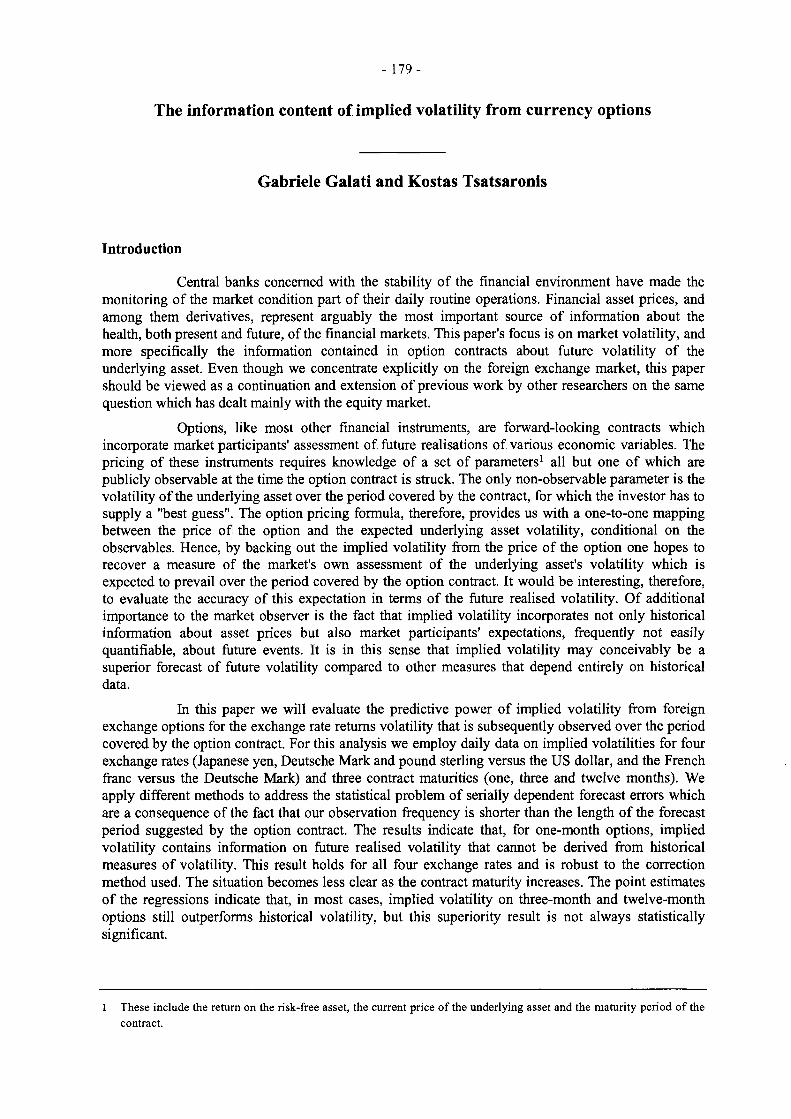
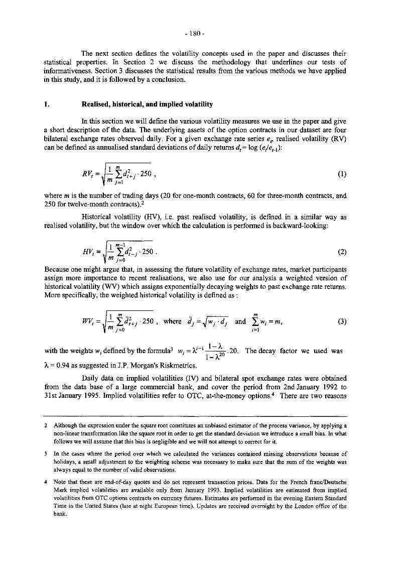
Figures 1-4 contain plots of the implied and realised volatilities as calculated by equation (1) for each currency and maturity in our dataset, and Table 1 presents summary statistics for the same series. A striking feature of implied and realised volatilities for all four exchange rates is that they become less variable as the maturity increases. This can be seen both from the standard deviations (one-month implied volatilities, for example, are two or three times as variable as twelvemonth implied volatilities) and from the range (the difference between the maximum and minimum) of the series, which decreases as the maturity increases.

Figure 5 plots the estimated autocorrelation and partial autocorrelation functions for the one-month implied and realised volatility series for all four exchange rates. From these plots one can conclude that these series can be reasonably characterised by pure autoregressive processes. In fact the estimated coefficient for the first order autoregressive term for the IV series ranges from 0.921 to 0.966, indicating a slow mean-reversion, with a half life of 8 to 20 trading days. For three of the exchange rates these coefficients are roughly the same for different maturities, indicating the same degree of persistence. The one exception is the yen/dollar rate, for which persistence seems to increase with the length of the contract.

Figure 5 also reveals a feature of the realised volatilities series that will be important for the design of our Monte Carlo experiment in Section 3. W e can see that the partial autocorrelation function shows significant jumps for lags that are roughly equal to the length of the option contract. The explanation for this phenomenon comes from the definition of R V and the way it is calculated over a moving time window of fixed length m. A shock to the exchange rate returns which occurs at time t will have a constant5 effect on the value o f R V for the next m-\ periods.

5 The effect is constant if we use the equally weighted scheme as in the formula (3). The effect of the shock will have an impact that dies out with time if the weighted RV is used instead. This is an additional reason why we look at weighted realised volatility series in addition to the unweighted ones.

- 1 8 2 -

Figure 1

Implied versus realised volatilities of the Yen/US dollar spot exchange rate

1-Month Contract

15-

7/10/92 1/01/92 14/07/93 20/04/94 25/01/95

3-Month Contract

1 6 - 1

14-

1 2 -

7/10/92 1/01/92 14/07/93 20/04/94 25/01/95

12-Month Contract

1 2 -

1 1 -

1 0 -

1/01/92 7/10/92 14/07/93 20/04/94 25/01/95

REALIZED - - IMPLIED

- 183 -

Figure 2

Implied versus realised volatilities of the DMAJS dollar spot exchange rate

1-Month Contract

25-

1 0 -

14/07/93 20/04/94 25/01/95 1/01/92 7/10/92

3-Month Contract

20

1 8 -

1 6 -

14-

1 2 -

1 0 -

25/01/95 7/10/92 14/07/93 20/04/94 1/01/92

12-Month Contract

' *A«'\ i ¡'r w.

k : i \ A "i ¡i'! "ir-iys W' V \ ; -J »

1/01/92 7/10/92 14/07/93 20/04/94 25/01/95

REALIZED --— IMPLIED

- 184-

Figure 3

Implied versus realised volatilities of the pound sterling/US dollar spot exchange rate

1 -Month Contract

25-,

2 0 -

1 0 -

1/01/92 7/10/92 14/07/93 20/04/94 25/01/95

3-Month Contract

14-

1 0 -

1/01/92 7/10/92 14/07/93 20/04/94 25/01/95

12-Month Contract

14-

1 2 -

1 0 -

1/01/92 7/10/92 14/07/93 20/04/94 25/01/95

REALIZED - - IMPLIED

- 185 -

Figure 4

Implied versus realised volatilities of the French franc/DM spot exchange rate

1 -Month Contract

1 0 -

1/01/92 7/10/92 14/07/93 20/04/94 25/01/95

3-Month Contract

10

8

6

4

2

0 - W T 1/01/92 7/10/92 14/07/93 20/04/94 25/01/95

12-Month Contract

3-

1/01/92 7/10/92 14/07/93 20/04/94 25/01/95

REALIZED - — IMPLIED

- 186-

Table 1

Descriptive statistics of volatilities

Variable Mean Standard deviation

Minimum Maximum

Yen/US doUar: 1-month IV 10.17 1.91 6.700 16.330 3-month FV 10.37 1.29 8.170 13.700 12-month IV 10.61 1.02 9.060 12.500

1-month RV 9.19 3.02 3.557 20.169 3-month RV 9.91 2.08 6.369 15.953 12-month RV 9.98 1.09 8.071 11.533

DM/US doUar: 1-month IV 11.89 2.39 7.540 22.000 3-month IV 12.01 1.63 8.900 18.240 12-month IV 12.09 0.78 10.580 13.980


Pound sterling/US dollar: 1-month IV 11.48 3.06 6.040 22.230 3-month IV 11.75 2.29 7.470 18.440 12-month IV 12.02 1.34 9.580 14.180


French franc/DM: 1-month TV 3.24 1.67 1.060 9.520 3-month IV 3.52 1.38 1.670 7.520 12-month IV 3.63 0.88 2.000 6.010


For all implied volatility series, as well as the underlying exchange rate returns, we estimated parsimonious time series models, and we report the results in Table 2. In selecting the most appropriate model for each series we have used a set of criteria. The first objective was to guarantee that the resulting errors were white noise, and the Box-Ljung test statistic was applied to detect serial correlation. The second consideration was to choose a model which fits the data well and is as parsimonious as possible. For this selection round the models that passed through our first filter were evaluated b y using the adjusted R 2 of the regression as well as the Akaike and Schwartz information criteria. Because Engle's (1982) Lagrange multiplier tests revealed the presence of conditional heteroskedasticity in the residuals, we estimated ARCH models of first or higher order to improve the ability of these models to represent the observed series. As Table 2 shows, implied volatilities are always represented by some autoregressive process and most series exhibit conditional heteroskedasticity in their residuals. It is comforting to note that the most representative model for the exchange rate returns by our criteria is consistent with economic theory which predicts that asset returns follow a random walk process with conditionally heteroskedastic errors.6

6 The exception is returns on the French franc/Deutsche Mark exchange rate, which follow a moving average process.

- 187 -

Figure 5

Estimated autocorrelation and partial autocorrelation functions for one-month contracts

One-month implied volatility One-month realised volatility

YEN/US$ YENAJSS

I I I I " I I 5 10 15 20 25 30 35 40 45 50 55 60 65

DM/US$

-0.2 5 10 15 20 25 30 35 40 45 50 55 60 65

DM/US$

1111111111111111 r 1111111 " 1111111 5 10 15 20 25 30 35 40 45 50 55 60 65 5 10 15 20 25 30 35 40 45 50 55 60 65

GBP/US$ GBPAJSS

• 11 • " i ••• 111» 1111 111111 M 1111 5 10 15 20 25 30 35 40 45 50 55 60 65 5 10 15 20 25 30 35 40 45 50 55 60 65

FFr/DM FFr/DM

M i i i I I I ' " I i i i ' I " i M ' 5 10 15 20 25 30 35 40 45 50 55 60 65

TTTTITT-5 10 15 20 25 30 35 40 45 50 55 60 65

1 A U T O C O R R E L A T I O N - P A R T I A L A U T O C O R R E L A T Ì Ó N I

- 188 -

Table 2

Time series representations of volatilities and exchange rate returns

Time series model ARCH effects

Implied volatilities Yen/US doUar:

1-month AR(3) ARCH(1) 3-month AR(3) ARCH(1) 12-month AR(2) ARCH(l)

DM/US doUar: 1-month AR(1) ARCH(3) 3-month AR(10) ARCH(3) 12-month AR(7) ARCH(3)

Pound sterling/US dollar: 1-month AR(5) ARCH(l) 3-month AR(6) ARCH(2) 12-month AR(8) ARCH(3)

French franc/DM: 1-month AR(6) ARCH(3) 3-month AR(6) ARCH(l) 12-month AR(5) ARCH(l)

Spot rate returns Yen/US dollar white noise -

DM/US dollar white noise ARCH(l) Pound sterling/US dollar white noise ARCH(6) French franc/DM white noise ARCH(1)

2. The information content of implied volatility

By definition, any random variable Xt observed at time t can be decomposed into two parts: its expected value conditional on an information set <bt_m available m periods earlier, and a zero mean forecast error e, which is uncorrelated with all information in the set In other words we can write:

Xt= E[Xt I d v J + e, where E[e, | O , . J = 0 .

Let us denote the forecast of Xt based on the informational set ®t_m as A statistical test of the rationality of this forecast could be easily conducted by means of the regression equation:7

Xt= a + ß • F(0 t_m) + e , . (4)

If F(0(_m) is an unbiased forecast of Xi one should expect the slope coefficient to be equal to one and the intercept term to be statistically indistinguishable from zero. Moreover, if one compares two different forecasts for Xt produced by conditioning on two information sets of which one is larger than the other, the forecast based on the smaller set should be inferior to the one based on the more inclusive one. More specifically, if FCOj) and F ( 0 2 ) represent two different forecasts of Xt and the

7 See, for example, Theil (1966).

- 189-

two information sets satisfy the relationship O j z) <I>2, then F(<&2) should not contain any information about Xt that is not already incorporated in In other words, OLS estimation of the following encompassing regression:

^ = a + ß F ( 0 1 ) + 7 F ( 0 2 ) + e i (5)

should yield that ß = 1 and 7 = 0, the reason being that the forecast based on the more inclusive information set should be more accurate and efficient predictor of fixture realisations than any forecast which is based on more restricted information (Fair and Schiller, 1990).

In what follows we apply this methodology to test for the accuracy of the implied volatility observed at the time the option contract is struck as a forecast of realised volatility as it is measured ex post over the contract's lifetime. If m is the length of the contract, then equation (4) becomes

RVt= a + ß • /F , + e , . (6)

As mentioned in the introductory section, implied volatility potentially incorporates information that is not strictly historical in nature but rather reflects the expected impact of anticipated future events on volatility.8 In this sense, it would be helpful to investigate the extent to which the past realised volatility is capable of predicting future levels of it, and use this as a benchmark for the measurement of the informativeness of implied volatility. To do this we first use historical volatility measured over the past period of length m as a predictor for RV and we evaluate its rationality by the conducting the same statistical tests as in the case of IV. More explicitly, we estimate by OLS the equation:9

RVt=a + § - HVt+zt (7)

and test for the hypothesis that a = 0 and ß = 1. We subsequently estimate the encompassing regression along the lines of equation (5), where IV represents the forecast based on the more inclusive information set and HV the one which is conditional on the smaller set which only includes historical realisations of the volatility process. A rejection of the statistical significance of the slope coefficient for the historical volatility should be interpreted as a sign that implied volatility is a superior forecaster for future volatility.

A further issue we explore is the dependence of implied volatility measures on the most recent history of actual volatility. We regress the IV at any given point in time against the historical realised volatility over the last period of length equal to the contract maturity, and test for the significance of the slope coefficient. The significance and the size of the slope coefficient from this regression will provide a measure of the closeness of the link between implied volatility and recent variability of the exchange rate returns.

Finally, in contrasting the informativeness of implied volatility measures to that of historical volatility we also conduct the above tests using measures of weighted historical volatility. The weighting scheme, which was described in the previous section, puts more emphasis on recent movements of the exchange rate returns at the expense of those in the more distant past.

8 A good example of such an event is a forthcoming election date that might have an impact on the expected volatility of the underlying asset. This election is an anticipated event that might not be reflected in the data up to the point where it is included in the period covered by the option contract.

9 The difference in the time subscript for the right-hand variables in equations (6) and (7) is due to the different definitions of these variables, as explained in the previous section.

- 190-

3. The empirical results

Previous empirical work assessing the predictive ability of implied for realised volatility -mostly conducted on stock price options - gives mixed results. Day and Lewis (1990) and Lamoureux and Lastrapes (1993) find that, over the short term, implied volatility contains a significant amount of information on future realised volatility. However, they find that implied volatility does not fully encompass the information provided by historical volatility. Canina and Figlewski (1993) conclude that implied volatility embedded in S & P 100 stock index options does not contain superior information to historical volatility. A recent study by the Bank of Japan (1995) looks at four types of contracts: options on the Nikkei 225, options on bond futures, options on short-term interest rate fixtures and currency options. It finds that IV contains unique and useful information about fixture volatility in the underlying assets in those markets where the trading volume is very large, such as the market for options on the Nikkei 225 and the market for one-month currency options. For longer-term currency options, IV has no significant explanatory power for future realised volatility.

A common econometric problem that these studies have to face is that the observation frequency (one day) is shorter than the period spanned by the options contracts (typically one-month or longer). Therefore, implied volatilities forecast actual volatility over overlapping periods, and as a consequence forecast errors are serially dependent, rendering the inference from standard statistical tests misleading.

To offer an illustration of this problem, let us examine it in the context of equation (4). The variable Xt and the forecast F ( 0 ; m) are observed in each and every period but not simultaneously. In fact, there are m periods that separate the formation of the forecast from the actual observation of the variable that is being forecast. By consequence, the forecast error et is not observed until period t (together with Xt) while the forecast was formed at period t-m. Now consider the forecasting exercise that takes place at the next period t-m+1 : the forecast for Xt+i is based on the information set

which does not include ef, and while the orthogonality properties of the optimal (linear) forecast still hold true there is no guarantee that the new forecast error will be uncorrelated with e, This problem will manifest itself every time a forecast is formed during the period covered by the original forecast horizon, that is for m-l periods in total. The forecast error therefore has an MA(/n-l) structure and this serial dependence of the residuals will bias downwards the variance of the coefficient estimates and invalidate any inference based on the traditional test statistics. For the remainder of this section we discuss various methods of addressing this problem.

3.1 Non-overlapping data

The simplest way to overcome the problem is to restrict the estimation to non-overlapping data by keeping in the sample only observations that are m periods apart. The obvious drawback of this approach is that, since only a small fraction of the available data is used, the econometrician voluntarily deprives him or herself of useful information. This reduction in the degrees of freedom has a clear and direct negative effect on the precision of the estimates. It is nonetheless worthwhile to perform the tests with the non-overlapping sample if only to use the results as a benchmark.

The results obtained for the two shorter maturity contracts are reported in Table 3. It was not possible with our dataset to run regressions with non-overlapping data for the twelve-month contracts. Also the lack of degrees of freedom suggests that even the results for three-month volatilities must be interpreted with great caution. Despite the above caveat, the regressions show that the intercept coefficient is always statistically significantly different from zero, a violation of the condition for efficient forecasts that requires it to be zero. We will restrict our more detailed discussion of the other results obtained from these regressions to the one-month maturity only.

- 191 -

Table 3

Regression results (non-overlapping data)

RVt=a + $*HVt+zt

Yen/US dollar: 1-month

3-month

DM/US dollar: 1-month

3-month

Pound sterling/US dollar: 1-month

3-month

French franc/DM: 1-month

3-month

a (p-value)

6.68 (0.00) 8.77

(0.03)

7.00 (0.00) 9.41

(0.04)

7.80 (0.00) 8.47

(0.08)

7.58 (0.00) 7.52

(0.04)

0.28

0.08

0.36

0.18

0.27

0.28

0.36

0.35

t-test of ß=0 (p-value)

1.80 (0.08) 0.22

(0.83)

2.36 (0.02) 0.55

(0.59)

1.75 (0.09) 0.81

(0.44)

2.53 (0.02) 1.48

(0.17)

t-test of P=1 (p-value)

4.74 (0.00) 2.70

(0.02)

4.17 (0.00) 2.59

(0.02)

4.66 (0.00) 2.11

(0.06)

4.49 (0.00) 2.71

(0.02)

adj. R 2

0.06

0.00

0.06

0.00

0.05

0.00

0.13

0.10

RVt = a + ß * IV,+ et

Yen/US doUar: 1-month

3-month

DM/US doUar: 1-month

3-month


3-month


3-month

a (p-value)

2.63 (0.27) 5.96

(0.28)

2.71 (0.42) 8.36

(0.24)

0.80 (0.75) 3.16

(0.55)

10.24 (0.00) 14.11 (0.04)

0.64

0.33

0.71

0.25

0.86

0.70

1.05

0.03


2.90 (0.01) 0.68

(0.51)

2.61 (0.01) 0.48

(0.64)

4.20 (0.00) 1.73

(0.12)

1.83 (0.08)

• 0 .02 (0.98)

t-test of ß= l (p-value)

1.64 (0.11) 1.41

(0.18)

1.09 (0.28) 1.40

(0.19)

0.66 (0.51) 0.74

(0.47)

0.09 (0.92)

• 0.76 (0.47)

adj. R 2

0.17

0.00

0.14

0.00

0.31

0.15

0.09

0.00

- 1 9 2 -

T a b l e 3 (cont . )

RVt= a + P*IVt + y*HVt + El


3-month


3-month


3-month


3-month

a (p-value)

2.58 (0.29) 6.07

(0.31)

3.29 (0.34) 8.59

(0.26)

0.87 (0.73) 3.27

(0.55)

8.69 (0.01) 14.82 (0.16)

0.67

0.37

0.50

0.11

0.92

0.92

0.99

0.06

0.03

0.05

0.17

0.13

0.07

0.23

0.12

0.04


2.15 (0.04) 0.63

(0.55)

1.30 (0.20) 0.14

(0.89)

3.65 (0.00) 1.51

(0.17)

1.67 (0.11)

• 0.04 (0.97)

t-test of 7=0 (p-value)

• 0.14 (0.89)

• 0.13 (0.90)

0.78 (0.44) 0.30

(0.77)

• 0.41 (0.68)

• 0.50 (0.63)

0.68 (0.51)

• 0.11 (0.92)

adj. R 2

0.14

0.00

0.13

0.00

0.29

0.08

0.06

0.00

/F,= a+ fi*HVt + et


3-month

DM/US dollar: 1-month

3-month

Pound sterling/US dollar 1-month

3-month


3-month

a (p-value)

6.11 (0.00) 7.35

(0.00)

7.48 (0.00) 7.46

(0.00)

7.36 (0.00) 5.41

(0.01)

2.66 (0.01) 3.73

(0.04)

0.45

0.36

0.39

0.42

0.38

0.57

0.04

0.01


6.06 (0.00) 2.20

(0.05 )

6.09 (0.00) 3.34

(0.01)

4.31 (0.00) 3.91

(0.00)

0.71 (0.48)

• 0 .06 (0.95)

t-test of ß = l (p-value)

7.27 (0.00) 3,91

(0.00)

9.49 (0.00) 4.60

(0.00)

7.14 (0.00) 2.93

(0.01)

15.87 (0.00) 10.30 (0.00)

adj. R 2

0.48

0.24

0.49

0.46

0.32

0.54

0.00

0.00

- 193 -

Table 3 (cont.)

RVt= a + P * WVt + zt

a (p-value) P



adj. R 2





6.49 (0.00)

7.06 (0.00)

8.18 (0.00)

8.32 (0.00)

0.29

0.36

0.24

0.30

2.05 (0.05)

2.27 (0.03)

1.51 (0.14)

2.19 (0.03)

4.95 (0.00)

4.01 (0.00)

4.77 (0.00)

5.21 (0.00)

0.08

0.10

0.03

0.09

RV ,= a + p * WVt + y*IVt+£t

a (p-value) P 1



adj. R 2





2.72 (0.26)

3.12 (0.36)

0.95 (0.71)

9.64 (0.00)

0.58

0.52

0.94

1.02

0.05

0.16

0.09

0.05

1.93 (0.06)

1.41 (0.17)

3.82 (0.00)

1.70 (0.10)

0.27 (0.79)

0.73 (0.47)

- 0.58 (0.57)

0.29 (0.77)

0.14

0.12

0.30

0.05

IVt= a + P * WVt + zt

a (p-value) P



adj. R 2





6.44 (0.00)

7.54 (0.00)

7.53 (0.00)

2.63 (0.01)

0.42

0.39

0.36

0.04

5.72 (0.00)

5.71 (0.00)

4.04 (0.00)

0.82 (0.42)

7.99 (0.00)

8.88 (0.00)

7.06 (0.00)

17.60 (0.00)

0.45

0.45

0.29

0.00

- 194-

For the one-month contract, implied volatility outperforms historical measures as a predictor of future volatility. In bivariate regressions with R V as the dependent variable, the coefficients on FV are significantly higher than those of HV. Coefficients on IV range from 0.64 to 1.05, and are highly significant for three out of four currency options, whereas coefficients on HV range between 0.28 and 0.36, and only in two cases are significant at the 5% level. The R 2 values are also at least two or three times higher in the regressions with IV as explanatory variable. Moreover, for all one-month options it is not possible to reject the hypothesis that ß = 1 for IV, while for H V this hypothesis is always rejected. However, joint tests for the hypothesis that forecasts are efficient and unbiased, i.e. for a = 0 and ß = 1, are always rejected.

When H V is added to IV as explanatory variable for RV, the coefficient on IV and the R 2

value remain roughly the same (the one exception being the Deutsche Mark/US dollar contract, where we see a substantial drop in the implied volatility slope coefficient) while the coefficient on HV becomes significantly smaller (and in some cases even negative).

Next, we regress IV on H V to measure the extent to which historical volatility explains realised volatility. Both the slope coefficients and the R 2 values for these regressions reported in Table 3 indicate that, with the exception o f the French franc/Deutsche Mark contracts, HV explains roughly between one-third and one-half o f the variation in IV. For all o f the above tests, the results are very similar when the weighted historical volatility is used in the place o f non-weighted H V as an explanatory variable.10

Based on this evidence, it is possible to conclude that, at least for one-month currency options, IV outperforms HV as a predictor o f future volatility of the exchange rate returns, although the hypothesis of efficient forecasts is rejected. This conclusion is consistent with the results reported b y the Bank of Japan (1995) study.

3.2 Asymptotic correction

The use of non-overlapping data eliminates the problem of serially correlated errors at the expense of a severe reduction in the degrees of freedom because o f the lower frequency of the data. For three-month options, it leaves only 11 observations over the whole three-year sample period, and there are not enough data points to test twelve-month volatilities. Even for one-month options, it leads to a significant reduction of power of the statistical tests as it discards 98% of the observations.

An alternative approach would be to deal with the serial correlation problem directly, and thus use the full set of available observations. Hansen and Hodrick (1980) have developed such a technique based on the method of moments estimation for the variance-covariance matrix of the coefficient estimates. Their method generates asymptotically consistent standard errors for the OLS estimates for the case of serial correlated regression residuals. White (1980) has improved on their method so that general forms of heteroskedasticity can be accommodated. Finally, because the above corrections do not always result in a positive definite variance-covariance matrix for the coefficient estimates, Newey and West (1987) offer a modification to deal with this problem.

We employ this procedure to perform hypothesis testing on regressions that use the full dataset of daily observations and we present the results in Table 4. With the use of the entire set of observations we can now focus with greater confidence on the three and twelve-month contracts. Although, b y and large, the results are in line with those obtained using non-overlapping data, Table 4 reveals some interesting facts. With respect to non-overlapping data, bivariate regressions for three-month options yield lower coefficients on H V and higher coefficients on IV. Moreover, the coefficient on IV is even higher when both IV and H V are used as explanatory variables. Results for twelve-

10 The different results for French franc/Deutsche Mark options might be at least in part explained by the much shorter sample for which data on implied volatilities for this exchange rate are available.

- 195 -

month options are difficult to interpret: the coefficients on H V range between - 0.81 and 0.74 and are always statistically significant, those on IV between - 0.35 and 0.37 and with one exception are never statistically significant. In regressions that include both HV and IV, coefficients on IV are significantly higher than those on H V and positive for all currencies except the yen/US dollar rate (for which the coefficient on IV is negative but not significant).

Table 4

Regression results (Hansen-Hodrick method)

RVt= a + $*HVt + zl

a ß t-test of a = 0

(p-value) t-test of ß=0

(p-value) t-test of ß= l

(p-value) adj. R 2

Yen/US doUar: 1-month 7.42 0.18 8.31

(0.00) 2.17

(0.04) 9.53

(0.00) 0.03

3-month 9.07 0.04 5.27 (0.00)

0.22 (0.83)

4.88 (0.00)

0.00

12-month 18.31 - 0.81 27.89 (0.00)

-11.99 (0.00)

-27.14 (0.00)

0.91

DM/US doUar: 1-month 7.53 0.31 5.97

(0.00) 3.10

(0.00) 6.86

(0.00) 0.10

3-month 9.96 0.13 4.41 (0.00)

0.79 (0.43)

5.17 (0.00)

0.01

12-month 1.96 0.68 1.76 (0.34)

7.63 (0.00)

2.29 (0.02)

0.34

Pound sterling/US dollar: 1-month 7.74 0.28 5.23

(0.00) 2.16

(0.03) 5.63

(0.00) 0.08

3-month 7.42 0.35 2.86 (0.00)

1.81 (0.07)

3.35 (0.00)

0.11

12-month 2.60 0.61 2.34 (0.04)

7.84 (0.00)

4.20 (0.00)

0.53

French franc/DM: 1-month 7.55 0.40 5.78

(0.00) 2.87

(0.00) 4.25

(0.00) 0.17

3-month 7.65 0.45 2.45 (0.01)

2.38 (0.02)

2.93 (0.00)

0.24

12-month 23.70 - 0.61 148.00 (0.00)

-30.16 (0.00)

-79.46 (0.00)

0.94

- 196-

Table 4 (cont.)

RVt= a + ß * I V t + zt

a ß t-test of a = 0

(p-value) t-test of ß=0

(p-value) t-test of ß = l

(p-value) adj. R 2

Yen/US dollar: 1-month 2.46 0.66 1.61

(0.11) 4.34

(0.00) 2.23

(0.03) 0.18

3-month 6.69 0.26 3.16 (0.00)

1.25 (0.21)

3.54 (0.00)

0.03

12-month 13.58 - 0.35 4.41 (0.00)

- 1.33 (0.18)

- 5.07 (0.00)

0.09

DM/US doUar: 1-month 2.71 0.70 1.19

(0.23) 3.77

(0.00) 1.59

(0.11) 0.18

3-month 7.12 0.35 2.17 (0.03)

1.45 (0.15)

2.66 (0.01)

0.03

12-month 7.44 0.37 1.07 (0.28)

0.73 (0.47)

1.24 (0.21)

0.03

Pound sterlingAJS dollar: 1-month 2.42 0.73 1.29

(0.20) 5.06

(0.00) 1.84

(0.07) 0.25

3-month 1.76 0.80 0.72 (0.47)

4.13 (0.00)

1.01 (0.31)

0.27

12-month 14.06 - 0.13 1.43 (0.15)

- 0.19 (0.85)

- 1.59 (0.11)

0.00

French franc/DM: 1-month 10.99 0.95 7.05

(0.00) 2.38

(0.02) 0.14

(0.89) 0.11

3-month 12.34 0.56 6.22 (0.00)

1.05 (0.29)

0.84 (0.40)

0.04

12-month 15.52 - 0.34 18.90 (0.00)

- 4.22 (0.00)

-16.48 (0.00)

0.05

- 197 -

Table 4 (cont.)

RVt= <*+ ß * / F , + 7 * # * ; + £,

a P y t-test of a=0 p-value

t-test of ß=0 p-value

t-test of 7=0 p-value

adj. R 2

Yen/US dollar: 1-month 1.79 0.97 - 0.28 1.13 4.19 - 2.33 0.24

(0.26) (0.00) (0.02) 3-month 6.83 0.36 - 0.12 3.07 1.32 - 0.47 0.03

(0.00) (0.17) (0.62) 12-month 18.30 0.00 - 0.81 14.95 - 0.00 -10.51 0.91

(0.00) (0.84) (0.00) DM/US doUar:

1-month 2.96 0.64 0.04 1.24 2.54 0.40 0.17 (0.21) (0.01) (0.69)

3-month 5.26 0.68 - 0.16 1.60 1.56 - 0.55 0.06 (0.11) (0.12) (0.58)

12-month - 1.48 0.65 0.34 - 0.46 1.18 1.28 0.48 (0.44) (0.15) (0.23)

Pound sterling/US dollar: 1-month 2.47 0.77 - 0.04 1.30 4.40 0.59 0.24

(0.19) (0.00) (0.77) 3-month 1.11 1.02 - 0.14 0.45 3.28 - 0.63 0.34

(0.65) (0.00) (0.53) 12-month - 0.73 0.70 0.19 - 1.17 5.38 2.36 0.74

(0.12) (0.00) (0.21) French franc/DM:

1-month 8.30 0.72 0.23 4.04 1.80 1.67 0.17 (0.00) (0.07) (0.09)

3-month 8.91 0.29 0.29 2.21 0.48 1.07 0.10 (0.02) (0.63) (0.28)

12-month 23.85 0.19 - 0.67 137.00 1.65 -21.07 0.93 (0.00) (0.10) (0.00)

- 198-

Table 4 (cont.)

IVt = a + HVt+zt

a ß

t-test of ß=0 t-test of ß = l adj. R 2

(p-value) ß (p-value) (p-value) adj. R 2

Yen/US dollar: 1-month 5.87

(0.00) 0.46 10.26

(0.00) 11.84 (0.00)

0.50

3-month 6.43 (0.00)

0.42 7.53 (0.00)

10.22 (0.00)

0.45

12-month 5.33 (0.00)

0.57 3.47 (0.00)

2.58 (0.01)

0.49

DM/US doUar: 1-month 7.04

(0.00) 0.43 5.24

(0.00) 7.02

(0.00) 0.52

3-month 6.92 (0.00)

0.43 6.47 (0.00)

8.43 (0.00)

0.66

12-month 7.26 (0.00)

0.39 7.31 (0.00)

11.52 (0.00)

0.62

Pound sterling/US dollar: 1-month 6.71

(0.00) 0.43 3.88

(0.00) 5.15

(0.00) 0.40

3-month 5.93 (0.00)

0.50 7.23 (0.00)

7.24 (0.00)

0.54

12-month 2.98 (0.00)

2.98 11.67 (0.00)

4.69 (0.00)

0.79

French franc/DM: 1-month 1.91

(0.00) 0.09 2.25

(0.02) 22.37 (0.00)

0.09

3-month 1.37 (0.14)

0.15 1.98 (0.05)

11.62 (0.00)

0.16

12-month 0.68 (0.51)

0.68 2.91 (0.00)

11.62 (0.00)

0.24

- 1 9 9 -

T a b l e 4 (con t . )

ÄF,= a + V*WVl + zl





a (p-value)

7.17 (0.00)

7.37 (0.00)

7.45 (0.00)

7.63 (0.00)

0.21

0.33

0.31

0.40


2.71 (0.01)

3.26 (0.00)

2.47 (0.01)

2.79 (0.01)


10.15 (0.00)

6.65 (0.00)

5.59 (0.00)

4.21 (0.00)

adj. R 2

0.05

0.11

0.10

0.17

RVt= <x+ ß * WVt + y*IVt+zl





a (p-value)

1.72 (0.29)

3.13 (0.18)

2.45 (0.19)

7.93 (0.00)

0.94

0.59

0.72

0.69

-0 .24

0.08

0.01

0.27


3.89 (0.00)

2.50 (0.01)

4.20 (0.00)

1.75 (0.08)


- 1.91 (0.06)

0.89 (0.37)

0.15 (0.88)

2.06 (0.04)

adj. R 2

0.23

0.17

0.24

0.07

IVt= a + ß * WVt + El



Pound sterling/US dollar 1-month


a (p-value)

2.46 (0.11)

2.71 (0.23)

2.42 (0.20)

10.99 (0.00)

0.66

0.70

0.73

0.95


4.34 (0.00)

3.77 (0.00)

5.06 (0.00)

2.38 (0.02)


2.23 (0.03)

1.59 (0.11)

1.84 (0.07)

0.14 (0.89)

adj. R 2

0.18

0.18

0.25

0.11

- 2 0 0 -

These results seem to indicate that, even for longer maturities, implied volatility can contain some information on future volatility additional to that contained in historical volatility. However, the difference in predictive power is less clear-cut than in the case of shorter maturity contracts. Moreover, the hypothesis that the IV provides an efficient and unbiased forecast for RV (i.e. that a = 0 and b= l ) is always rejected for all maturities.

When IV is regressed on HV, both the slope coefficient and the R 2 values increase (in some cases substantially) with respect to regressions on non-overlapping observations. Furthermore, there is a tendency for the explanatory power of HV to rise as the maturity of the option contracts increases, indicating that over longer horizons the historical volatility of the underlying contract is the dominant factor affecting implied volatility. Interestingly, the coefficient on weighted historical volatilities rises sharply with respect both to regressions on simple historical volatilities and to regressions on weighted volatilities that use non-overlapping data. At the same time, however, the value of the R 2 decreases significantly.

3.3 Monte Carlo simulations

Mishkin (1990) argues that, although the Hodrick-Hansen-White-Newey-West method allows correct inference asymptotically, the finite sample distributions of the test statistics may differ significantly from the asymptotic distribution. Huizinga and Mishkin (1984) find that the difference between sample distributions and asymptotic distributions can be quite large in cases where there is a large data overlap (i.e. when the forecast horizon becomes large compared to the sample size). To control for the effects of this small-sample bias we performed a Monte Carlo simulation to generate empirical distributions for the test statistics which are then used to compute critical values and marginal significance levels.

The procedure consists of three stages. In the first stage, we searched for a parsimonious time series representation for the series involved in the regressions, as detailed in Section 1. While the implied volatility series did not present any particular problem, the realised volatility series could not be modelled directly for reasons that have to do with the way they are defined, as discussed above. We have opted to model the daily exchange rate returns instead, for which we obtained very reasonable representations.

In the second stage we simulated implied volatilities and exchange rate returns using the estimated model coefficients and randomly generated errors series. Subsequently, we computed the realised volatility for the simulated daily returns series. We used the actual series realisations as initial values to start each process, and generated five years of data before the start of the sample that was actually used in the regressions, in order to minimise the impact of the initial conditions.

Finally, at the last stage we ran the same OLS regressions using the simulated series to produce test statistics for the hypothesis that the coefficient is equal to zero. These regressions were run over samples of the same size as the original ones and the resulting distributions of the t-statistics were used to calculate the empirical significance levels for the OLS t-statistics for the actual regressions.

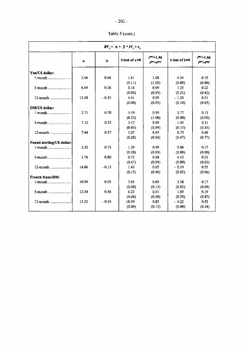
Table 5 contains the results of this Monte Carlo simulation. For each regression coefficient, we report the probability,11 according to the empirical distribution, that we observe a t-statistic value greater than the one that corresponds to the 5% significance level (i.e. Pr[/mc> 1.96]). If there is no problem with the sample size, this probability should be approximately equal to 5%, so any deviation from this number should be interpreted as a failure of the asymptotic correction to perform satisfactorily in samples as small as ours. We also report the empirical probability value for

11 The calculation of the probability is simply the ratio of occurrences divided by the number of Monte Carlo trials: in our case 1,000.

-201 -

the observed t-statistic (i.e. Pr[imc> r^]). The null hypothesis that the slope coefficient is equal to zero is rejected when this probability value is smaller than the chosen significance level.

Table 5 shows several interesting results. First, implied volatility is always highly significant when equation (6) is tested for one-month contracts (and in the case of the pound sterling/US dollar returns also for the three-month contracts) using the empirical distributions. However, in contradiction to the results obtained with the asymptotic distributions, the null hypothesis that b=l is generally rejected.12

Table 5

Monte Carlo results

RVt= a + $*HVt + et

a b t-test of a=0 rc>i.96 f"c>tasy t-test of b=0

<"'>1.96 fnc>tasy

Yen/US dollar: 1-month 7.42 0.18 8.31 1.00 2.17 0.14

(0.00) (0.75) (0.04) (0.11) 3-month 9.07 0.04 5.27 1.00 0.22 0.23

(0.00) (0.80) (0.83) (0.86) 12-month 18.31 -0.81 27.89 0.97 -11.99 0.76

(0.00) (0.17) (0.00) (0.14) DM/US doUar:

1-month 7.53 0.31 5.97 1.00 3.10 0.12 (0.00) (0.99) (0.00) (0.02)

3-month 9.96 0.13 4.41 1.00 0.79 0.24 (0.00) (0.91) (0.43) (0.63)

12-month 1.96 0.68 1.76 0.95 7.63 0.75 (0.34) (0.96) (0.00) (0.27)

Pound sterling/US dollar: 1-month 7.74 0.28 5.23 1.00 2.16 0.29

(0.00) (0.93) (0.03) (0.22) 3-month 7.42 0.35 2.86 1.00 1.81 0.17

(0.00) (0.99) (0.07) (0.20) 12-month 2.60 0.61 2.34 0.95 7.84 0.73

(0.04) (0.94) (0.00) (0.26) French franc/DM:

1-month 7.55 0.40 5.78 0.96 2.87 0.26 (0.00) (0.21) (0.00) (0.04)

3-month 7.65 0.45 2.45 0.87 2.38 0.29 (0.01) (0.82) (0.02) (0.46)

12-month 23.70 -0.61 148.00 0.93 -30.16 0.75 (0.00) (0.03) (0.00) (0.05)

12 These results are not reported in the table.

- 2 0 2 -

Table 5 (cont.)

RVt= a + ß * I V t + e ,

a b t-test of a=0 <""^1.96 t-test of b=0 ^ > 1 . 9 6

Yen/US doUar: 1-month 2.46 0.66 1.61 1.00 4.34 0.15

(0.11) (1.00) (0.00) (0.00) 3-month 6.69 0.26 3.16 0.99 1.25 0.22

(0.00) (0.99) (0.21) (0.42) 12-month 13.58 -0.35 4.41 0.99 - 1.33 0.51

(0.00) (0.95) (0.18) (0.65) DM/US doUar:

1-month 2.71 0.70 1.19 0.99 3.77 0.13 (0.23) (1.00) (0.00) (0.00)

3-month 7.12 0.35 2.17 0.99 1.45 0.21 (0.03) (0.99) (0.15) (0.35)

12-month 7.44 0.37 1.07 0.95 0.73 0.48 (0.28) (0.96) (0.47) (0.77)

Pound sterling/US dollar: 1-month 2.42 0.73 1.29 0.99 5.06 0.17

(0.20) (0.99) (0.00) (0.00) 3-month 1.76 0.80 0.72 0.98 4.13 0.23

(0.47) (0.99) (0.00) (0.03) 12-month 14.06 -0.13 1.43 0.95 - 0.19 0.55

(0.15) (0.96) (0.85) (0.96) French franc/DM:

1-month 10.99 0.95 7.05 0.89 2.38 0.17 (0.00) (0.15) (0.02) (0.09)

3-month 12.34 0.56 6.22 0.91 1.05 0.19 (0.00) (0.30) (0.29) (0.87)

12-month 15.52 -0.34 18.99 0.82 - 4.22 0.53 (0.00) (0.12) (0.00) (0.24)

-203 -

Table 5 (cont.)

RVt= a + ß * IV^^HV, +e,

a ^ > 1 . 9 6 ß *">1.96 Y <"">1.96 t-test of a=0 t-test of b=0 t-test of g =0 fiti^fosy

Yen/US doUar: 1-month 1.79 0.97 - 0.28

1.13 1.00 4.19 0.16 - 2.33 0.15 0.26 1.00 0.00 0.00 0.02 0.10

3-month 6.83 0.36 - 0.12 3.07 0.98 1.32 0.26 - 0.47 0.29 0.00 0.91 0.17 0.43 0.62 0.79

12-month 18.30 0.00 - 0.81 14.95 0.97 -0.00 0.56 -10.51 0.78 0.00 0.43 0.84 1.00 0.00 0.21

DM/US doUar : 1-month 2.96 0.64 0.04

1.24 0.99 2.54 0.14 0.40 0.12 0.21 1.00 0.01 0.07 0.69 0.73

3-month 5.26 0.68 - 0.16 1.60 0.96 1.56 0.28 - 0.55 0.30 0.11 0.98 0.12 0.37 0.58 0.78

12-month - 1.48 0.65 0.34 -0.46 0.94 1.18 0.55 1.28 0.75

0.44 0.99 0.15 0.73 0.23 0.86 Pound sterlingAJS dollar:

1-month 2.47 0.77 - 0.04 1.30 0.98 4.40 0.14 0.59 0.23 0.19 0.98 0.00 0.00 0.77 0.80

3-month 1.11 1.02 - 0.14 0.45 0.96 3.28 0.28 - 0.63 0.25 0.65 1.00 0.00 0.08 0.53 0.72

12-month -0.73 0.70 0.19 - 1.17 0.94 5.38 0.61 2.36 0.75

0.12 0.97 0.00 0.22 0.21 0.70

French francA>M: 1-month 8.30 0.72 0.23

4.04 0.82 1.80 0.14 1.67 0.23 0.00 0.36 0.07 0.23 0.09 0.07

3-month 8.91 0.29 0.29 2.15 0.82 0.48 0.34 1.07 0.36 0.02 0.84 0.63 0.87 0.28 0.55

12-month 23.85 0.19 - 0.67 137.00 0.90 1.65 0.55 -21.07 0.78

0.00 0.001 0.10 0.39 0.00 0.10

Tests of the same hypothesis in the context of equation (7), that is when RV is the forecasting variable, reveal that the coefficient on historical volatility is significant only for the one-month Deutsche Mark/US dollar options. This contradicts the results obtained with asymptotic distributions which indicated that historical volatility was significant for all exchange rates and at almost all maturities.

- 2 0 4 -

Finally, when both implied and historical volatilities are simultaneously included in the encompassing regression, we find that only the coefficient on implied volatility is statistically significant. The probability value for IV is less than 1% for yen/US dollar and pound sterling/US dollar options, and around 7% for Deutsche Mark/US dollar options, while for HV it is close to 10% for yen/US dollar options and around 70-80% for the other options.13 The conclusion based on asymptotic distributions that the negative coefficients on HV in the equations for yen/US dollar and French franc/Deutsche Mark options are statistically significant is therefore incorrect.

These results reinforce the earlier conclusion that for the one-month contract implied volatility has a significant predictive power for future volatility, and that its predictive ability is superior that of historical volatility. For the three-month and the twelve-month options, the coefficients on both historical and implied volatility are generally not statistically significant in equations (8) and (10). This indicates that, at longer horizons, neither historical nor implied volatility seem to perform well as predictor of future volatility. Moreover, the tests reject the hypothesis of unbiased and efficient forecasts, i.e. that a = 0 and b = 1, for all maturities.

The above conclusions regarding the informational content of implied volatility for future realisations of volatility are, of course, subject to the caveats we mentioned in Section 1 above when we referred to the possibility that the IV figures we use may actually underestimate the true market expectation for the exchange rate return volatility. However we should note that, even if this bias is sizable, it will only tend to strengthen our rejection of the hypothesis that IV is an unbiased and efficient predictor of RV, as the estimated slope coefficient would be higher with the conventional measure of IV than with the more accurate one.

Conclusions

This paper uses daily data on four currency options at three different maturities to address the question of how well implied volatility from currency options can predict future volatility of the underlying exchange rate returns and whether the information it provides is superior to that contained in past realised volatility. We find that, at the shorter end of the maturity spectrum, implied volatility performs well in forecasting future volatility, and that implied volatility contains information that goes beyond what we can infer from past realised volatility. However, we reject the hypothesis that implied volatility represents an unbiased and efficient forecast of future volatility. Over longer horizons, we find that neither implied nor historical volatility provides a good forecast of future volatility.

We also find that results obtained with simple OLS regressions are misleading because of the serial correlation of the forecast errors. Using an asymptotically valid method may not solve this problem because of the insufficient number of available observations. To allow correct inference, we therefore use a Monte Carlo method to generate empirical distributions of the relevant test statistics. The Monte Carlo results largely confirm our conclusions regarding the informativeness of the one-month options but are not as clear for the longer maturity contracts.

Overall we can say that the monitoring of the movements in the implied volatility of foreign exchange contracts can be a useful tool for the anticipation of periods of instability in these markets. However, the information content of implied volatility quickly deteriorates with the length of the contract and it can only be used in the very short horizon. Further work is required in order to establish a firmer relationship between implied and realised volatility, especially in the periods that precede large movements of the underlying exchange rates.

13 The lower the probability value the higher the significance of the coefficient.

-205 -

References

Bank of Japan (1995): "Empirical analyses of the information content of implied volatility", Bank of Japan Quarterly Bulletin, February.

Campa, J.M. and P.H.K. Chang (1994): "Testing the expectations hypothesis on the term structure of volatilities in foreign exchange options", mimeo, Stem School of Business, New York University (forthcoming Journal of Finance).

Canina, L. and Stephen Figlewski (1993): "The information content of implied volatility", The Review of Financial Studies, 1993, 6 (3), pp. 659-681.

Day, T.E. and C.M. Lewis (1990): "Stock market volatility and the information content of stock index options", Journal of Econometrics, 52, pp. 267-287.

Fair, R.C. and Robert J. Shiller (1990): "Comparing information in forecasts from econometric models", American Economic Review, 80, pp. 375-389.

Hansen, L.P. and R.J. Hodrick (1980): "Forward exchange rates as optimal predictors of future spot rates: an econometric analysis", Journal of Political Economy, 88.

Huizinga, J. and F.S. Mishkin (1984): "Inflation and real interest rates on assets with different risk characteristics", Carnegie-Rochester Conference Series on Public Policy, 24, pp. 231-274.

Lamoureux, C.G. and W.D. Lastrape (1993): "Forecasting stock return variance: toward an understanding of stochastic implied volatilities", Review of Financial Studies, 6, pp. 293-326.

Mishkin, F.S (1990): "What does the term structure tell us about fixture inflation?", Journal of Monetary Economics, 25, pp. 77-95.

Newey, W.K. and K.D. West (1987): "A simple, positive definite heteroscedasticity and autocorrelation consistent covariance matrix", Econometrica, 55, pp. 703-708.

Theil, (1966): Applied Economic Forecasting, North-Holland, Amsterdam.

White, H. (1980): "A heteroscedasticity-consistent covariance matrix estimator and direct tests for heteroscedasticity", Econometrica, 48, pp. 817-838.

the information content of implied volatility from ... · pdf file- 179-the information...

Documents