The Input-Output Structural DecompositionAnalysis of “Flexible” Production Systems

Carlo Milana∗

Forthcoming in Michael L. Lahr and Erik Dietzenbacher (eds), Input-OutputAnalysis: Frontiers and Extensions, Essays in honor of Ronald E. Miller, London:Macmillan Press, 2001.

∗ Istituto di Studi e Analisi Economica, Piazza dell’Indipendenza, 4, 00185 Rome, Italy.

2

The Input-Output Structural DecompositionAnalysis of “Flexible” Production Systems

Carlo Milana∗

Abstract

Decomposition techniques in the input-output analysis are traditionally based on theassumption that the elasticity of price-induced input substitution is either zero (the Leontiefassumption) or equal to one (the Cobb-Douglas and Klein-Morishima assumption).Sectoral differences in quantities or prices that are observed over time or across space areaccordingly decomposed into direct and indirect input-quantity or input-price componentsand technological change effects. Since the empirical results may depend significantly onthe underlying hypothesis on price-induced input substitution, the paper is aimed atextending the traditional input-output model to a more general production system that iscompatible with all possible values of elasticities of substitution. Assuming quadraticpolynomial functional forms of sectoral cost functions, a more general input-outputaccounting system can be developed. In this paper, the traditional input-output model isimplicitly extended to the case of Translog cost functions by using Törnqvist indexnumbers in interspatial and intertemporal comparisons of relative price levels and theircomponents. A new decomposition procedure is derived and applied empirically. Theresults are compared with those obtained by using the traditional input-outputdecomposition procedures.

1 Introduction

The input-output structural decomposition analysis (IO SDA) is traditionally used tostudy the observed changes in the level and mix of output and employment. Thesechanges, often defined as “structural transformation” of the economy, are decomposedinto changes in technology, changes in final demand and changes in import dependence.Examples of decomposition of intertemporal changes in sectoral outputs that areobserved in single countries are given by Skolka (1989) and Rose and Chen (1991). Fora critical review of theoretical and empirical developments of the IO SDA see Rose andCasler (1996).

∗ Istituto di Studi e Analisi Economica, Piazza dell’Indipendenza, 4, 00185 Rome, Italy.

3

The IO SDA can also be applied to the dual input-output system of prices toaccount for the output-price variations that are observed over time or across space.Examples are given by Karasz (1992) in the intertemporal comparison of price relativelevels in one single country and Fujikawa, Izumi and Milana (1995a, 1995b) in theanalysis of inter-country price differences. Another instance of IO SDA is given byDietzenbacher (1999), where intertemporal and inter-country variations of sectoraloutput values are decomposed into price and quantity components, which in turn arefurther decomposed into basic structural elements.

An important feature of the IO SDA is its capability of distinguishing the directand indirect components of the observed sectoral changes by combining proceduressimilar to growth accounting with the techniques of input-output analysis. Thismethodology is particularly suitable to account for the indirect effects on one industryof structural and productivity changes that take place in other industries and aretransmitted by these industries through the supplied intermediate inputs. Hulten (1978),for example, has stressed the distinction between “productivity change originating in asector and the impact of productivity change on the sector” through intermediate inputscoming from other sectors (see Hulten, 1978, p. 511; italics in the original text). Thesetwo types of technological impacts combined together make up what he called the“effective” rate of technical or productivity change. Producer price variations can be,therefore, decomposed into primary-input price components and direct and indirecttotal-factor-productivity components.

The distinction of the direct elements of costs of production from direct-and-indirect primary factor-input costs is grounded on the different concepts of “industry”and “vertically integrated sector”. The industry can be defined as a production activityusing directly intermediate inputs and primary factor inputs. The vertically integratedsector is an accounting entity to which are attributed the costs of primary inputs that areused directly by the examined industry and the costs of primary inputs that are requireddirectly and indirectly to produce all the intermediate inputs that are supplied to thatindustry by other industries. The distinction of these two concepts is clearly defined inthe field of input-output analysis and is well known in the general economic literature(see, for example, Pasinetti, 1973 for an extensive discussion of these concepts).

Many IO SDA studies have, however, recognized that there is no uniquepossible way to decompose changes of output prices and quantities that are observedover discrete time or across space. In fact, significantly different empirical results havebeen noted among various alternative procedures. Vaccara and Simon (1968), amongthe early studies that used the technique of IO SDA, were well aware of this outcome,while Fromm (1968), in his comment on their paper, mentioned index numberproblems. More recently, some contributions were focused on the analysis of sensitivityof results obtained by alternative procedures (see, for example, Dietzenbacher and Los,1997, 1998, who examined a large set of possibilities).

Changes in output prices or quantities are usually studied in the field of IO SDAin terms of differences rather than ratios. For this reason, interpretations of the resultsobtained by several alternative procedures from the viewpoint of index number theoryare not straitforward. Moreover, the index number approach by itself is not consideredto be very useful when the indirect effects that arise from the interindustry relations areto be taken into account. Rose and Casler (1996, p. 38), for example, in their discussionof the state of the art in this area point out: “The major difference between IO SDA and

4

the index number approach is the inability of the index number approach to incorporateindirect and induced effects into the analysis. [...] Whether or not the index numberapproach can be broadened to the full scope of IO SDA by incorporating other inputsand explicitly analyzing substitution and productivity effects is open to question”.

The accounting procedures that are employed in IO SDA studies are usuallyconfined to restrictive hypotheses concerning the observed technological changes.Following Leontief’s (1936, 1941) original contributions, it is usually assumed that theinput-output ratios remain fixed in physical terms when relative input prices change or,alternatively, following Klein (1952-53, 1956) and Morishima (1956, 1957), it issometimes assumed that input-output value shares, evaluated at current prices, remainfixed as relative input prices change. These two alternative approaches can be justifiedex ante under the hypothesis that the underlying cost functions have Leontief and Cobb-Douglas functional forms, implying that the elasticities of price-induced inputsubstitution are equal to zero and one, respectively. The input-output decompositionprocedures that are based on these interpretations are constructed by using fixed-weighted Laspeyres-, Paasche-, and Cobb-Douglas-type formulas. However, thesedifferent formulas yield generally different results.

The hypothesis of invariant input-output ratios with respect to input-pricechanges can also be justified ex post on the ground of the non-substitution theorem,which establishes that, under certain conditions, changes in composition of finaldemand do not bring about changes in relative input prices and input requirements perunit of output, either in physical terms or in value shares, even if input substitution isfeasible when input prices change. However, although the implications of the non-substitution theorem turn out to be convenient for simulation purposes, the invariabilityof input-output ratios (valued at constant or current prices) with respect to changes incomposition of final demand is by no means necessary in the ex-post accountinganalysis and may yield unrealistic results.

In this paper, the IO SDA is applied to output price changes focusing on priceratios rather than price differences. It introduces the use of Törnqvist index numberswithin the input-output framework to decompose changes in output prices into directand indirect components of costs. The results are compared with those that are obtainedby applying the traditional Laspeyres, Paasche and Cobb-Douglas index numbers. TheTörnqvist index number belongs to the class of index numbers that Diewert (1976) hasdefined “superlative”. These are “exact” for second-order approximating functionalforms of cost or production functions in the sense that they give the same results thatcould be obtained by using these functions directly. They are also able to exhibit a widerange of degrees of price-induced input substitution and are therefore more general thanthe Leontief and Cobb-Douglas functional forms. In particular, the Törnqvist indexnumber is “exact” for the Translog functional form. It has been widely applied ingrowth accounting studies and intertemporal and interspatial comparisons of directcomponents of costs of production at the industry level since the pioneering works ofDale W. Jorgenson and his associates1.

1 The methodology of the decomposition analysis based on Törnqvist index numbers was originatedby Jorgenson and Nishimizu (1978), and was further applied in a number of important studies (see alsoJorgenson, Kuroda and Nishimizu, 1987 and Jorgenson and Kuroda, 1990).

5

The paper proceeds as follows. The next section presents the point of view ofthe economic theory of index numbers on why and in what direction alternativedecompositions of output-cost (or price) variations may differ. In the third section, theindex number approach is integrated into the scheme of the IO SDA of output-costchanges by using alternative functional forms that correspond to different hypotheseson the structure of technology. The fourth section compares the empirical results of thealternative index numbers that are applied in an interspatial decomposition of pricedifferences between Japan and the US in 1985 and an intertemporal decomposition ofprice changes that were observed in the US between 1985 and 1990. The fifth sectionconcludes.

2 The decomposition of cost changes from the viewpoint ofthe economic theory of index numbers

The observed variations in sectoral output prices over time or across space can bedecomposed into input-price effects and effects due to changes in technology, scale ofproduction and non competitive or disequilibrium extra-profits. Variations over time oracross space in output prices can be decomposed by referring to the direct elements ofcost of production at the industry level by using cost functions, if the functional formsand parameters of these functions are known, or index numbers that are “exact” for thesame cost functions. It should be emphasized that accounting for indirect componentsof cost variations that are embodied into the intermediate-input costs is ruled out usingthis approach alone2.

Diewert (1976) showed that an index number is “exact” for a specific functionalform of the cost function if it is identically equal to the ratios of values obtained byusing the cost function directly. However, when the cost function is not known, we canat best establish only the upper and/or lower bounds for possible values of the “true”unknown index number, and the choice of the index number formula is critical,especially when there is a significant difference in the results obtained by usingdifferent functional forms. The discussion that follows in this section will help us tounderstand the nature of the no-unique solution problem in decomposition analysesfrom the viewpoint of the economic theory of index numbers3.

Let us assume that the long-run total cost function of the jth industry at theobservation point (a region or a time period) τ can be represented as follows:

2 In fact, this approach can deal with only the direct elements of costs (and their variations), sincefurther decompositions of the direct intermediate-input costs cannot be performed without using an input-output technique.

3 For surveys of the economic theory of index numbers, see Frisch (1936), Allen (1949), Samuelson andSwamy (1974), and Diewert (1981).

6

C y yj j j j j jj

τ τ τ τ τ τ τ ττ ψ( , ) min :w w X X

X≡ ⋅ ≥ d io t (1)

where wτ is the (N+M)-order row vector of N intermediate-input prices and M primary-

factor input prices, Xτj is the (N+M)-order column vector of direct requirements of the

N intermediate inputs and M primary factors at the output level yτj, ψτ

j(Xτ

j) is the

industry j's production function, which satisfies the usual regularity conditions.The long-run average cost function of the jth industry at the observation point τ is

therefore

c yC y

yj jj j

j

τ τ ττ τ τ

τ( , )( , )

ww

≡

which, under constant returns to scale, reduces to cτj(wτ), since in this case C

τj(wτ,yτ

j) ≡

yτj c

τj(wτ). By Shepherd's lemma, the cost-minimizing input requirements per unit of

output or direct input-output coefficients are given by x X wwjj

jj

j jy yC yτ

ττ

ττ τ τ≡ = ∇1 1( , )

and, since Cτj(wτ,yτ

j) is linearly homogeneous in wτ, by Euler's theorem,

C y C yj j j jτ τ τ τ τ τ τ( , ) ( , )w w ww= ⋅∇ , hence c

τj(wτ,yτ

j) = wτ⋅⋅ xτ

j .

The theory of the input price and quantity indexes is largely isomorphic to themore widely studied theory of the cost-of-living index, where the so-called Konüs trueindex number of cost of living and the Allen index number of aggregate real inputs areconstructed by using expenditure or cost functions4. Similarly, in the context of theproduction activity, the index numbers of aggregate input prices are theoretically basedon the use of the cost function. As the theory of the cost of living has clearly shown,there is no unique way of accounting for the intertemporal or interspatial cost changes.Alternative decomposition procedures are equally possible, among which are thefollowing (the subscript indicating the jth industry is omitted to simplify notation)5:

c y c y Pt t tL K d P A d( , ) / ( , ) /, ,w w0 0 0 = − −π (2)

c y c y Pt t tP K d L A d( , ) / ( , ) /, ,w w0 0 0 = − −π (3)

c y c y Pt t tF K d F A d( , ) / ( , ) /, ,w w0 0 0 = − −π (4)

whereP c y c yL K d

t− ≡, ( , ) / ( , )0 0 0 0 0w w : Laspeyres-Konüs-type index number of

aggregate direct-input prices;π P A d

t t t tc y c y− ≡, ( , ) / ( , )0 0w w : Paasche-Allen-type index number of direct

productivity effects;

4 The basic contributions to the theory of aggregate input-price and input-quantity indexes in the contextof production activities were given by Muellbauer (1972), Blackorby, Schwarm and Fisher (1986),Diewert (1987), and Fisher (1988).

5 See, for example, Diewert (1981, pp. 170-174) for the definitions of these index numbers.

7

P c y c yP K dt t t t t

− ≡, ( , ) / ( , )w w0 : Paasche-Konüs-type index number of aggregate

direct-input prices;π L A d

t tc y c y− ≡, ( , ) / ( , )0 0 0 0w w : Laspeyres-Allen-type index number of direct

productivity effects;

P P PF K d L K d P K d− − −≡ ⋅, , ,

/1 2: Fisher-Konüs-type index number of aggregate

direct-input prices;

π π πF A d L K d P K d− − −≡ ⋅, , ,

/1 2: Fisher-Allen-type index number of direct

productivity effects.Under the assumption of cost minimization, the economic theory of index

numbers implies that c yt t0 0 0( , )w w x≤ ⋅ and c yt t t( , )w w x0 0≤ ⋅ , which leads us tothe following bounds for the input-price indexes:

Pc y

c y

c yL K d

t t

− ≡ =⋅,

( , )

( , )

( , )0 0

0 0 0

0 0

0 0

ww

ww x

≤ w xw x

t

L dP⋅⋅

≡0

0 0 , (5)

Pc y

c y c yP K d

t t t

t t

t t

t t− ≡ = ⋅,

( , )

( , ) ( , )

ww

w xw0 0

≥ w xw x

t t

t P dP⋅⋅

≡0 , (6)

where PL d, and PP d, are, respectively, the Laspeyres and Paasche index numbers of

aggregate input prices.Similarly, the following bounds can be established for the productivity indexes:

π L A d t t t t

c y

c y c y− ≡ = ⋅,

( , )

( , ) ( , )

0 0 0

0

0 0

0

ww

w xw

≥ w xw x

0 0

0

⋅⋅

≡t L dπ , (7)

π P A d

t

t t t

t

t t

c y

c y

c y− ≡ =

⋅,

( , )

( , )

( , )0 0 0 0ww

ww x

≤ w xw x

t

t t P d

⋅⋅

≡0

π , (8)

where π L d, and π P d, are, respectively, the Laspeyres and Paasche direct productivity

index numbers.If the cost functions c0( )⋅ and ct ( )⋅ are non-homothetic to each other, then both

cases where PL d, ≥ PP d, and PL d, ≤ PP d, are possible. When, instead, the cost

functions c0( )⋅ and ct ( )⋅ are homothetic to each other, then the Laspeyres input-priceindex is the upper bound and the Paasche input-price index is the lower bound of theinterval of possible values of the Konüs-type input-price index number, that is

P P PL d L K d P d, , ,≥ ≥− (9)

P P PL d P K d P d, , ,≥ ≥− (10)

8

as shown by Frisch (1936) for the theory of cost-of-living index.It can be noted that the reciprocals of productivity index numbers correspond to

the index numbers of aggregate input quantities. Fisher (1988) pointed out that, whilethe cost function and the Konüs-type input-price indexes are always homogeneous ofdegree one in the input prices, the Paasche-Allen-type index number of real aggregateinputs given by π P A d−

−,

1 is not, in general, homogeneous of degree one in the input

quantities, that is if x xt = ⋅λ 0 , where λ is a positive scalar, then

c y c yt t t t( , ) / ( , )w w0 0 ≥ λ in view of (8). Similarly, we can show that the Laspeyers-

Allen-type index number of real aggregate inputs given by π L A d−−

,1 is not, in general,

homogeneous of degree one in the input quantities, that is if x xt = ⋅λ 0 , then

c y c yt t( , ) / ( , )w w0 0 0 0 ≤ λ , in view of (7). In contrast, a desirable property of the

index number of real aggregate inputs is that when all the current-period inputs areequal to the base-period inputs multiplied by the same scale factor λ , also this indexshould result to be equal exactly to λ . When this property is not met, a Fisher-Allen-type index of productivity should be preferred. In fact, the index π

F A d−

−,

1 does not

generally turn out to be homogeneous of degree one in the input quantities, but being ageometric mean of π L A d−

−,

1 and π P A d−−

,1 , it has a homogeneity closer to degree one than

these two last indexes. As we shall see, in particular cases of the underlying costfunctions, the Fisher-Allen-type productivity index number π F A d− , and its input-price

counterpart PF A d− , can be computed on the basis of the theory of exact index numbers

using only the observed input prices and quantities.

3 Integrating the index number approach into the I-Ostructural decomposition analysis

Different specifications of production technology implying, in particular,different degrees of price-induced input substitution, are reflected by differentfunctional forms of cost functions. In this section, alternative functional forms will beconsidered as approximations to the unknown sectoral cost functions and theircorresponding index numbers are used within the framework of the input-outputsystem. In the light of the IO SDA, the search for the appropriate functional forms ofprice equations should take into account the feasibility of computation, not only ofdirect effects of input prices and productivity, but also of indirect effects that areincorporated into the prices of intermediate inputs. The chosen functional forms enableus to specify systems of equations which are linear or log-linear in prices. Linearity inprices or in their logarithmic transformation is necessary for the algebraic derivation ofthe indirect effects by means of the reduced linear form of the model. The first twoassumptions considered here concern the Leontief and Cobb-Douglas functional formsthat are commonly used by traditional input-output decomposition analyses, whereasthe third assumption, which makes up the major novelty of this paper, uses the Translog

9

functional form as a second-order approximation to the (unknown) cost functions andtakes advantage of the linearity of the corresponding Törnqvist index numbers in thelogarithmic changes of prices.

3.1 Using the Leontief functional form

The original Leontief's (1936, 1941) input-output model has been formulatedunder the assumption of physical input-output coefficients that remain fixed as relativeinput prices and the output level change. The elasticity of price-induced inputsubstitution is, therefore, equal to zero and every variation in the input-outputcoefficients is attributed to productivity change. The corresponding minimum averagecost function of the jth industry at the observation point τ under constant returns toscale is the following6:

c j j jLτ τ τ τ τ τ( )w p a v f≡ ⋅ + ⋅ ∀ j (11)

where wτ ≡ [p

τ v

τ], pτ is the N-order row vector of sectoral output prices (and

intermediate-input prices net of indirect taxes, transportation costs and commercialmargins), vτ is the M-order row vector of primary factor prices (including indirect taxeson intermediate inputs), a j

τ and f jτ are, respectively, the N-order and M-order column

vectors of the direct input-output coefficients in physical or constant-price valued termsfor intermediate inputs and primary factors. With zero extra-profits, the output price isequal to the average total cost of production. In matrix notation, the whole system ofprice equations based on cost accounting at the industry level is, therefore, thefollowing:

p p A v Fτ τ τ τ τ= ⋅ + ⋅ (12)

where Aτ and Fτ are, respectively, the matrices of direct input-output coefficients inphysical or constant-price valued terms for intermediate inputs and primary factors.

Solving (12) with respect to the output prices yields the following system ofprice equations based on cost accounting at the level of vertically integrated sectors:

p v F I Aτ τ τ τ= ⋅ ⋅ − −( ) 1 (13)

Variations in output prices over time or across space can be defined in terms ofratios7. Starting from (12) these ratios can be decomposed into the index numbers ofdirect input-price and technology components as follows:

6 The particular Leontief functional form defined by (11) has a linear polynomial form and, therefore,can be seen as a first-order approximation to the unknown average cost function.

7 Variations in output prices can be defined in terms of price differences rather than price ratios. Thedecomposition of price differences requires, however, accounting methods that are different from those

10

p p P PtL d P d P d L d⋅ = ⋅ = ⋅− − −( $ ) $ $

, , , ,0 1 1 1π π (14)

where ^ means that a vector is transformed into a diagonal matrix and

P p A v F pL dt t

, ( $ )≡ + ⋅ ⋅ −0 0 0 1 : vector of sectoral Laspeyres index numbers of

aggregate direct-input prices,

π P dt t t

, ( $ )≡ + ⋅ ⋅ −p A v F p0 0 1 : vector of sectoral Paasche index numbers of

direct productivity effects,

P p A v F pP dt t t t t

,,( $ )≡ + ⋅ ⋅ −0 1 (where p p A v F0 0 0,t t t≡ + ⋅ ): vector of sectoral

Paasche index numbers of aggregate direct-input prices,

π L dt

,,( $ )≡ + ⋅ ⋅ −p A v F p0 0 0 0 0 1 : vector of sectoral Laspeyres index numbers of

direct productivity effects.

It can be noted that π P d, = P p pL dt

L d, ,$ ( $ ) ~⋅ ⋅ ≡− −0 1 1π and π L d, =

P p pP dt

, $ ( $ )⋅ ⋅ ≡− −0 1 1 ~,π P d , where ~

,π L d and ~,π P d are, respectively, vectors of implicit

Laspeyres and implicit Paasche index numbers of direct productivity effects. (The tilde~ indicates that the Laspeyres and Paasche index numbers of productivity effects areimplicitly defined, that is they are respectively derived as ratios between the Laspeyresand Paasche input-price index numbers and the output-price index.)

Under the hypothesis that the sectoral cost functions have the Leontieffunctional form (11) with the input-output coefficients equal to those that are observedat point 0, the Laspeyres input-price index defined in (14) has the meaning of aLaspeyres-Konüs-type index number. If the reference input-output coefficients are thosethat are observed at point t, the Paasche input-price index has the meaning of a Paasche-Konüs-type index number. Note also that the reciprocals of the Laspeyres and Paascheindex numbers of productivity representing the index numbers of real aggregate inputshave the ideal property of homogeneity of degree one in the input quantities.

Starting from (13), the output-price ratios can be decomposed into indexnumbers of direct-and-indirect primary-input price and technology components asfollows:

p p P PtL d i P d i P d i L d i⋅ = ⋅ = ⋅− − −( $ ) $ $

, & , & , & , &0 1 1 1π π (15)

where

P v F I A pL d it

, & ( ) ( $ )≡ ⋅ − ⋅− −0 0 1 0 1 : vector of sectoral Laspeyres index numbers

of direct-and-indirect primary-input prices,

π P d it t

, & ( ) ( $ )≡ ⋅ − ⋅− −v F I A p0 0 1 1 : vector of sectoral Paasche index numbers of

direct-and-indirect productivity effects,

considered here. Examples of these methods, which are based on index number theory, are given byFujikawa, Izumi, and Milana (1985a) and Diewert (1998).

11

P v F I A pP d it t t t

, &,( ) ( $ )≡ ⋅ − ⋅− −1 0 1 (where p v F I A0 0 1, ( )t t t≡ ⋅ − − : vector of

sectoral Paasche index numbers of direct-and-indirect primary-input prices,

π L d it

, &,( ) ( $ )≡ ⋅ − ⋅− −v F I A p0 0 0 1 0 1 : vector of sectoral Laspeyres index numbers

of direct-and-indirect productivity effects.

It can be noted that π P d i, & = P p pL d it

L d i, & , &$ ( $ ) ~⋅ ⋅ ≡− −0 1 1π and π L d i, & =

P p pP d it

, & $ ( $ )⋅ ⋅ ≡− −0 1 1 ~, &π P d i , where ~

, &π L d i and ~, &π P d i are, respectively, vectors of

implicit Laspeyres and implicit Paasche index numbers of direct and indirectproductivity effects.

The indexes of indirect productivity effects on output prices can be defined byconsidering the direct-and-indirect productivity component of changes in the directintermediate-input prices as follows:

π L it t t

,,( ) ( $ )≡ ⋅ − + ⋅ ⋅− −v F I A A v F p0 0 0 1 0 0 1 (with p 0,t ≡ v F I A A0 1⋅ − −t t t( ) +

v F0 ⋅ t ): vector of sectoral Laspeyres-type index numbers of indirect productivity

effects,

π P it t t

,,( ) ( $ )≡ ⋅ − + ⋅ ⋅− −v F I A A v F p0 0 1 0 0 0 1 (with p t ,0 ≡ v F I A At t t⋅ − −( ) 1 0 +

v Ft ⋅ 0 ): vector of sectoral Paasche-type index numbers of indirect productivity effects.

A number of considerations can be made on the indirect productivity effects andinput-price indexes. First, the indexes of indirect productivity effects can be derivedfrom the two productivity indexes defined above, that is π π πL i L d i L d, , & ,

$= ⋅ −1 and π P i, =

π P d i, & ⋅ −$

,π P d1 .

Second, the indirect productivity effects turn out to be included, at the industrylevel, into the aggregate direct input price indexes PL d, and PP d, . They are instead

excluded, at the level of vertically integrated sectors, from the aggregate direct-and-indirect primary-input price indexes PL d i, & and PP d i, & . The ratios of the latter to the

former input-price indexes are equal to indirect-productivity indexes, that is

P PL d i L d P i, & , ,$⋅ =−1 π and P PP d i P d L i, & , ,

$⋅ =−1 π . This means that, rearranging terms, the

former indexes can be obtained by correcting the latter indexes for indirect productivityeffects, that is P PL d L d i P i, , & ,

$= ⋅ −π 1 and P PP d P d i L i, , & ,$= ⋅ −π 1 .

Third, the distinction between the two types of input-price indexes stems fromthe decomposition of the direct intermediate-input prices into incorporated primary-input prices and incorporated productivity effects.

3.2 The Klein-Morishima assumption

Klein (1952-53, 1956) and Morishima (1956, 1957) have reinterpretedLeontief's input-output model assuming that the functional form of sectoral productionfunctions are Cobb-Douglas rather than linear Leontief. The elasticity of price-inducedinput substitution is, therefore, assumed to be equal to one and input-output coefficientsin physical terms can vary accordingly, not only because of productivity change, but

12

also because of changes in relative input prices. With the additional assumptions ofconstant returns to scale and competitive zero extra-profits that are necessary to ease adirect comparison with Leontief's original model8, this formulation leads us to thestandard Cobb-Douglas sectoral cost equation9:

ln ( ) ln lnc aCDj j pj vjτ τ τ τ τw p a v f≡ + ⋅ + ⋅0 ∀ j (16)

where a j0τ is a variable scale factor, depending on technology, a pj and fvj are vectors

of input-output shares at current prices that are assumed to be fixed with respect tochanges in relative prices.

In long-run competitive equilibrium, the output price is equal to the averagetotal cost of production under constant returns to scales. In matrix notation, the wholesystem of price equations in logarithmic terms is the following:

ln ln lnp a p A v Fτ τ τ τ= + ⋅ + ⋅0 p v (17)

where

A p A pp ≡ ⋅ ⋅ −$ ( $ )τ τ τ 1 (18)

F w F pv ≡ ⋅ ⋅ −$ ( $ )τ τ τ 1

The current-price input-output matrices A p and Fv are invariant with respect to

changes in relative input prices, whereas the physical input-output coefficient matricesAτ and Fτ vary appropriately as relative input prices change.

The reduced form of (17) is given by

ln ln ( ) ( )p v F I A a I Aτ τ τ= ⋅ − + ⋅ −− −v p p

10

1 (19)

If a0τ is not known, the vector a I A0

1τ ⋅ − −( )p representing the technological impact on

the sectoral price levels at the observation point τ can be calculated implicitly as a

residual given by ln ln ( )p v F I Aτ τ− ⋅ − −v p

1 .

Taking account of (17), output-price ratios can be decomposed into directcomponents of input-price and productivity effects as follows:

p p PtCD d CD d⋅ = ⋅− −( $ ) ~$

, ,0 1 1π (20)

8 These assumptions are by no means necessary in this analytical context, although non-constant returnsto scale and rewards to scale factors require a more complex accounting system.

9 The particular Cobb-Douglas functional form defined by (16) has a log-linear polynomial form and,therefore, can be seen as a first-order approximation to the unknown average cost function.

13

where

P v v F p p ACD dt

vt

p, exp (ln ln ) (ln ln )≡ − ⋅ + − ⋅0 0 : vector of sectoral Cobb-

Douglas index numbers of aggregate direct-input prices,~ ( $ ) exp (ln ln ) (ln ln ) (ln ln ), ,π CD d CD d

t tv

tp

t≡ ⋅ ⋅ = − ⋅ + − ⋅ − −− −P p p v v F p p A p p0 1 1 0 0 0

= exp ( )− −a a0 00t : vector of sectoral (implicit) Cobb-Douglas index numbers of direct

productivity effects. (The tilde ~ indicates that the Cobb-Douglas index number isimplicitly defined, that is it is derived as a ratio between the Cobb-Douglas input-priceindex number and the output-price index.)

Under the hypothesis that the cost function has the Cobb-Douglas functionalform (16) with the input-cost shares being equal to those that are observed at point 0,the input-price and productivity indexes defined in (20) have the meaning of Laspeyres-Konüs-type and Paasche-Allen-type index numbers, respectively. They have, instead,the meaning of Paasche-Konüs-type and Laspeyres-Allen-type index numbers,respectively, if the reference input cost shares are those that are observed at point t.Moreover, the technological changes that are considered by the Cobb-Douglasfunctional form of the price equation (16) are homothetic. Hence, the reciprocal of theCobb-Douglas productivity index representing the index number of real aggregateinputs has the ideal property of homogeneity of degree one in input quantities.

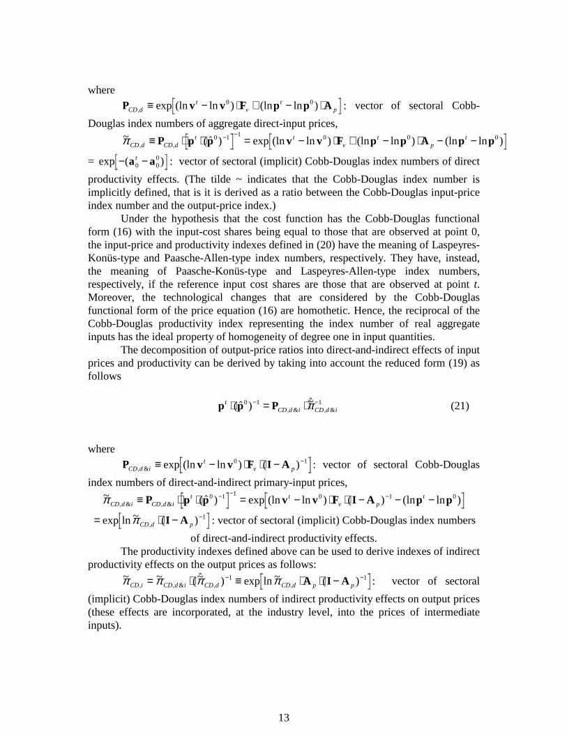
The decomposition of output-price ratios into direct-and-indirect effects of inputprices and productivity can be derived by taking into account the reduced form (19) asfollows

p p PtCD d i CD d i⋅ = ⋅− −( $ ) ~$

, & , &0 1 1π (21)

where

P v v F I ACD d it

v p, & exp (ln ln ) ( )≡ − ⋅ ⋅ − −0 1 : vector of sectoral Cobb-Douglas

index numbers of direct-and-indirect primary-input prices,~ ( $ ) exp (ln ln ) ( ) (ln ln ), & , &π CD d i CD d i

t tv p

t≡ ⋅ ⋅ = − ⋅ ⋅ − − −− − −P p p v v F I A p p0 1 1 0 1 0

= ⋅ − −exp ln ~ ( ),π CD d pI A 1 : vector of sectoral (implicit) Cobb-Douglas index numbers

of direct-and-indirect productivity effects. The productivity indexes defined above can be used to derive indexes of indirectproductivity effects on the output prices as follows:

~ ~ (~$ ) exp ln ~ ( ), , & , ,π π π πCD i CD d i CD d CD d p p= ⋅ ≡ ⋅ ⋅ −− −1 1A I A : vector of sectoral

(implicit) Cobb-Douglas index numbers of indirect productivity effects on output prices(these effects are incorporated, at the industry level, into the prices of intermediateinputs).

14

The Cobb-Douglas direct input-price components can be obtained fromcorrecting the direct-and-indirect primary input-price components for the indirect-

productivity effects on output prices, that is P PCD d CD d i CD i, , & ,~$= ⋅ −π 1 .

3.3 The Translog generalization

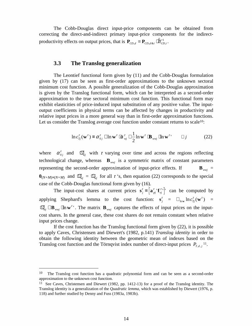
The Leontief functional form given by (11) and the Cobb-Douglas formulationgiven by (17) can be seen as first-order approximations to the unknown sectoralminimum cost function. A possible generalization of the Cobb-Douglas approximationis given by the Translog functional form, which can be interpreted as a second-orderapproximation to the true sectoral minimum cost function. This functional form mayexhibit elasticities of price-induced input substitution of any positive value. The input-output coefficients in physical terms can be affected by changes in productivity andrelative input prices in a more general way than in first-order approximation functions.Let us consider the Translog average cost function under constant returns to scale10:

ln ( ) ln ln ln 'cTj j wj wwjτ τ τ τ τ τ ταw w w B w≡ + ⋅ + ⋅ ⋅0

1

2α ∀ j (22)

where α τ0 j and awj

τ with τ varying over time and across the regions reflecting

technological change, whereas Bwwj is a symmetric matrix of constant parameters

representing the second-order approximation of input-price effects. If Bwwj =

0(N+M)×(N+M) and awjτ = awj for all τ ‘s, then equation (22) corresponds to the special

case of the Cobb-Douglas functional form given by (16).

The input-cost shares at current prices s a fj pj vjτ τ τ≡ ' ' ' can be computed by

applying Shephard's lemma to the cost function: s jτ = ∇ln ln ( )w wcTj

τ τ =

awj wwjτ τ+ ⋅B wln ' . The matrix Bwwj captures the effects of input prices on the input-

cost shares. In the general case, these cost shares do not remain constant when relativeinput prices change.

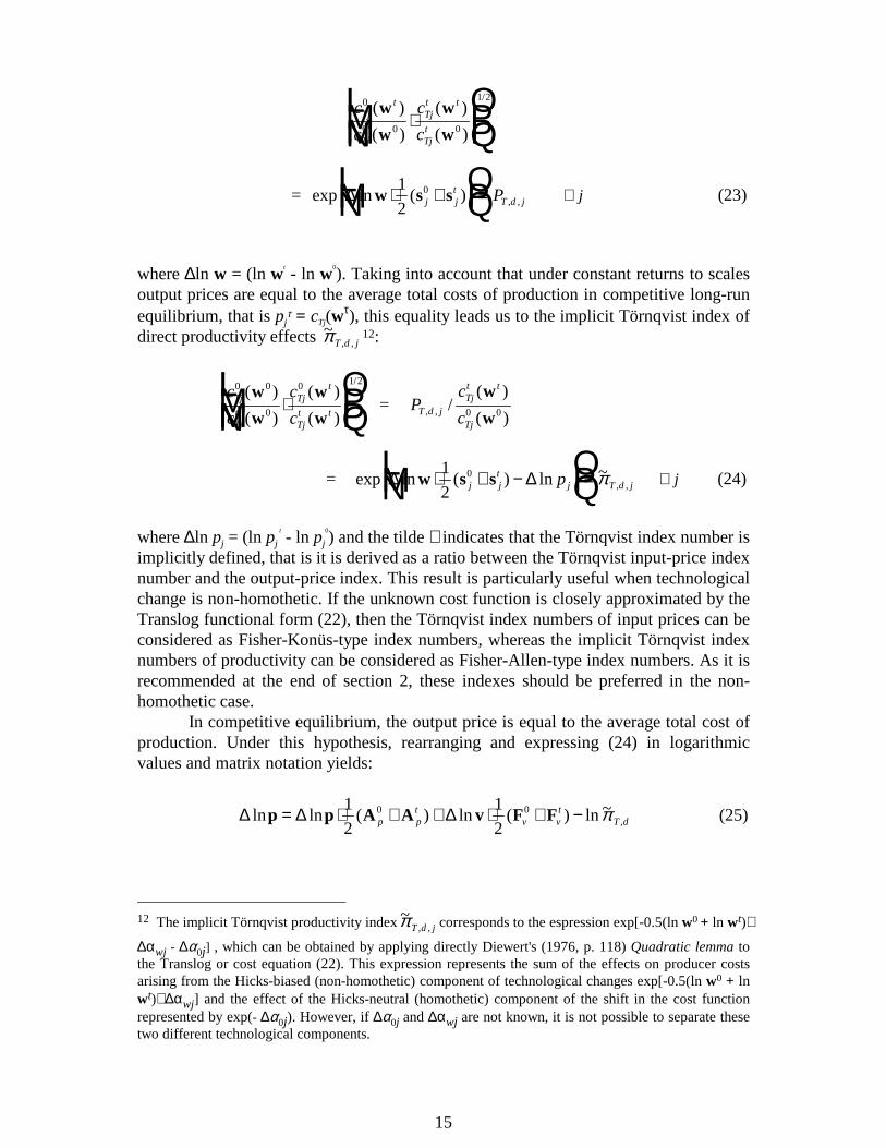
If the cost function has the Translog functional form given by (22), it is possibleto apply Caves, Christensen and Diewert's (1982, p.141) Translog identity in order toobtain the following identity between the geometric mean of indexes based on theTranslog cost function and the Törnqvist index number of direct-input prices PT d j, ,

11.

10 The Translog cost function has a quadratic polynomial form and can be seen as a second-orderapproximation to the unknown cost function.11 See Caves, Christensen and Diewert (1982, pp. 1412-13) for a proof of the Translog identity. TheTranslog identity is a generalization of the Quadratic lemma, which was established by Diewert (1976, p.118) and further studied by Denny and Fuss (1983a, 1983b).

15

c

c

c

cTj

t

Tj

Tjt t

Tjt

0

0 0 0

1 2( )

( )

( )

( )

/w

w

w

w⋅

LNMM

OQPP

= exp ln ( ) , ,∆ w s s⋅ +LNM

OQP≡1

20j j

tT d jP ∀ j (23)

where ∆ln w = (ln wt

- ln w0

). Taking into account that under constant returns to scalesoutput prices are equal to the average total costs of production in competitive long-runequilibrium, that is pj

τ = cTj(wτ), this equality leads us to the implicit Törnqvist index of

direct productivity effects ~, ,π T d j

12:

c

c

c

cTj

Tjt

Tjt

Tjt t

0 0

0

0 1 2( )

( )

( )

( )

/w

w

w

w⋅

LNMM

OQPP

= Pc

cT d jTjt t

Tj, , /

( )

( )

w

w0 0

= exp ln ( ) ln ~, ,∆ ∆w s s⋅ + −L

NMOQP≡1

20j j

tj T d jp π ∀ j (24)

where ∆ln pj = (ln pj

t

- ln pj

0

) and the tilde ∼ indicates that the Törnqvist index number isimplicitly defined, that is it is derived as a ratio between the Törnqvist input-price indexnumber and the output-price index. This result is particularly useful when technologicalchange is non-homothetic. If the unknown cost function is closely approximated by theTranslog functional form (22), then the Törnqvist index numbers of input prices can beconsidered as Fisher-Konüs-type index numbers, whereas the implicit Törnqvist indexnumbers of productivity can be considered as Fisher-Allen-type index numbers. As it isrecommended at the end of section 2, these indexes should be preferred in the non-homothetic case.

In competitive equilibrium, the output price is equal to the average total cost ofproduction. Under this hypothesis, rearranging and expressing (24) in logarithmicvalues and matrix notation yields:

∆ ∆ ∆ln ln ( ) ln ( ) ln ~,p p A A v F F= ⋅ + + ⋅ + −1

2

1

20 0p p

tv v

tT dπ (25)

12 The implicit Törnqvist productivity index ~

, ,π T d j corresponds to the espression exp[-0.5(ln w0 + ln wt)⋅

∆αwj - ∆α0j] , which can be obtained by applying directly Diewert's (1976, p. 118) Quadratic lemma tothe Translog or cost equation (22). This expression represents the sum of the effects on producer costsarising from the Hicks-biased (non-homothetic) component of technological changes exp[-0.5(ln w0 + lnwt)⋅ ∆αwj] and the effect of the Hicks-neutral (homothetic) component of the shift in the cost functionrepresented by exp(- ∆α0j). However, if ∆α0j and ∆αwj are not known, it is not possible to separate thesetwo different technological components.

16

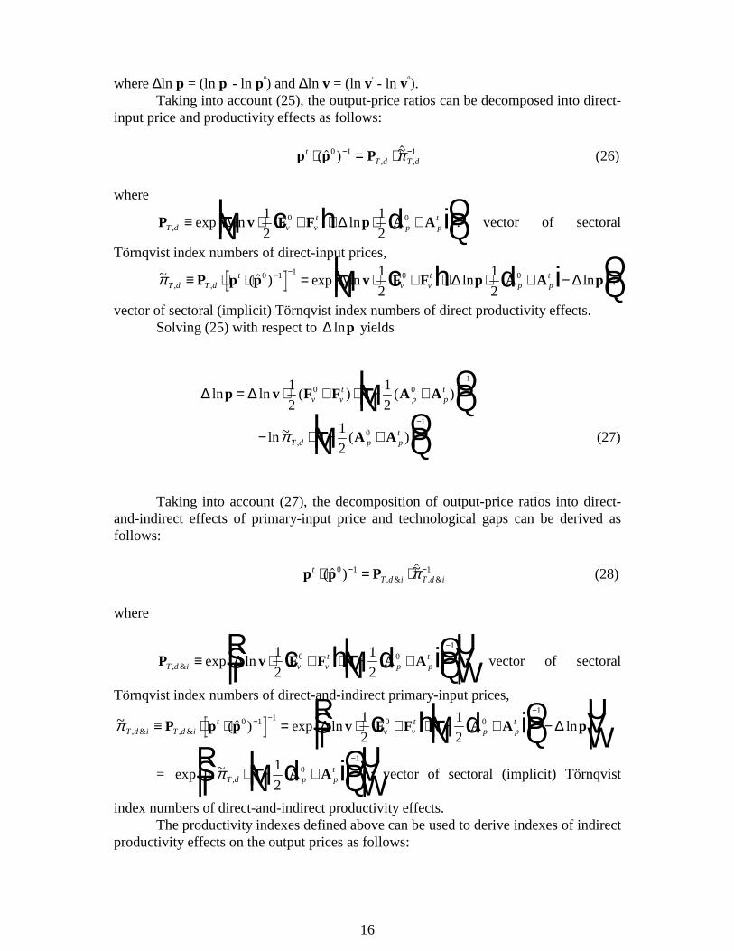
where ∆ln p = (ln pt

- ln p0

) and ∆ln v = (ln vt

- ln v0

).Taking into account (25), the output-price ratios can be decomposed into direct-

input price and productivity effects as follows:

p p PtT d T d⋅ = ⋅− −( $ ) ~$

, ,0 1 1π (26)

where

P v F F p A AT d v vt

p pt

, exp ln ln≡ ⋅ + + ⋅ +LNM

OQP∆ ∆1

2

1

20 0c h d i : vector of sectoral

Törnqvist index numbers of direct-input prices,

~ ( $ ) exp ln ln ln, ,π T d T dt

v vt

p pt≡ ⋅ ⋅ = ⋅ + + ⋅ + −L

NMOQP

− −P p p v F F p A A p0 1 1 0 01

2

1

2∆ ∆ ∆c h d i :

vector of sectoral (implicit) Törnqvist index numbers of direct productivity effects.Solving (25) with respect to ∆ lnp yields

∆ ∆ln ln ( ) ( )p v F F I A A= ⋅ + ⋅ − +LNM

OQP

−1

2

1

20 0

1

v vt

p pt

− ⋅ − +LNM

OQP

−

ln ~ ( ),π T d p ptI A A

1

20

1

(27)

Taking into account (27), the decomposition of output-price ratios into direct-and-indirect effects of primary-input price and technological gaps can be derived asfollows:

p p PtT d i T d i⋅ = ⋅− −( $ ) ~$

, & , &0 1 1π (28)

where

P v F F I A AT d i v vt

p pt

, & exp ln≡ ⋅ + ⋅ − +LNM

OQP

RS|T|UV|W|

−

∆ 1

2

1

20 0

1

c h d i : vector of sectoral

Törnqvist index numbers of direct-and-indirect primary-input prices,

~ ( $ ) exp ln ln, & , &π T d i T d it

v vt

p pt≡ ⋅ ⋅ = ⋅ + ⋅ − +L

NMOQP−

RS|T|UV|W|

− −−

P p p v F F I A A p0 1 1 0 01

1

2

1

2∆ ∆c h d i

= exp ln ~,π T d p p

t⋅ − +LNM

OQP

RS|T|UV|W|

−

I A A1

20

1

d i : vector of sectoral (implicit) Törnqvist

index numbers of direct-and-indirect productivity effects.The productivity indexes defined above can be used to derive indexes of indirect

productivity effects on the output prices as follows:

17

~ ~ ~ exp ln ~, , & , ,π π π πT i T d i T d T d p p

tp p

t= ⋅ = ⋅ + ⋅ − +LNM

OQP

RS|T|UV|W|

−−

1 0 01

1

2

1

2A A I A Ad i d i : vector of

sectoral (implicit) Törnqvist index numbers of indirect productivity effects on outputprices (these effects are directly and indirectly incorporated, at the industry level, intothe prices of intermediate inputs).

The Törnqvist direct input-price components can be obtained from correctingthe direct-and-indirect primary input-price components for the indirect-productivity

effects on output prices, that is P PT d T d i T d, , & ,~$= ⋅ −π 1 .

4 Empirical applications to interspatial and intertemporalcomparisons

In this section, the four alternative procedures based on the Laspeyres-, Paasche-,Cobb-Douglas-, and Törnqvist-type formulas are used to decompose the sectoraloutput-price variations that were observed between two countries in a given year, Japanand the US in 1985, and between the US in 1985 and the US in 1990. The examinedprocedures are, therefore, evaluated at both the interspatial and intertemporaldimensions. A brief description of the data used is given before presenting the empiricalresults.

4.1 Data

The input-output tables of the Japanese economy in 1985 and the US economyin 1985 and 1990 have been derived from the OECD (1995) input-output database. TheOECD input-output tables are constructed at current and constant prices at the level ofdisaggregation of 35 industries that are defined according to the International StandardIndustrial Classification, Revision 2 (ISIC, Rev. 2). The number of industries in theinput-output tables actually used has been reduced to 22 because some of the industrieshave been aggregated together to meet the availability of data on relative price levels.The sectoral output-price ratios between Japan and the US in 1985 have beenconstructed by using the information on the Purchasing Power Parity (PPP) data thathas been kindly provided by the Statistical Division of the OECD for the year 1985 atthe most disaggregated level (187 commodities). These data were aggregated andcorrected by “peeling off” indirect taxes, transportation costs and commercial margins.The sectoral import-price ratios have been constructed by using the availableinformation on values and quantities of external trade flows. The output- and import-price indexes of the US in 1990 relative to the US in 1985 have been directly obtainedas implicit deflators of the current- and constant-price values of the OECD input-outputtables. The sectoral data on the US labor-input prices and labor compensation havebeen calculated on the basis of the national accounts, since the OECD input-outputtables of the US do not disaggregate value added into labor and capital costs. The inputs

18

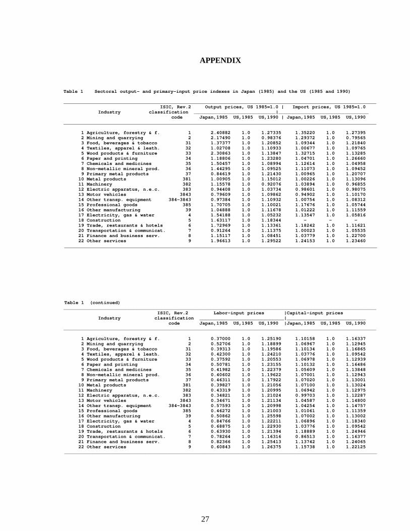
of labor services have been computed by deflating labor compensation by means ofindexes of labor-input prices. The sectoral capital-input prices have been calculatedfollowing the rental-price approach, which, in its simplest form, defines the price ofcapital services as the product of the expected long-run real interest rate plus adepreciation rate and the purchase price of the investments goods. The inputs of capitalservices have been derived by deflating the operating surplus by means of rental priceindexes under the assumption of constant returns to scale and zero extra-profits. Theconstructed sectoral output- and input-price data are shown in Table 1 in the Appendix.

4.2 Sources of output price changes

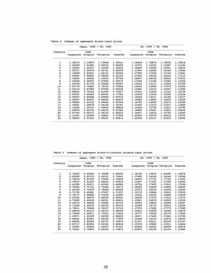
The observed variations in the output prices between Japan and the US in 1985and between the US in 1985 and the US in 1990 have been decomposed into aggregatedinput-price indexes and indexes of productivity effects. Tables 1 to 6 in the Appendixpresent the results obtained by using the four alternative formulas of Laspeyres, Cobb-Douglas, Törnqvist, and Paasche index numbers. A number of important elementsemerge from their analysis.

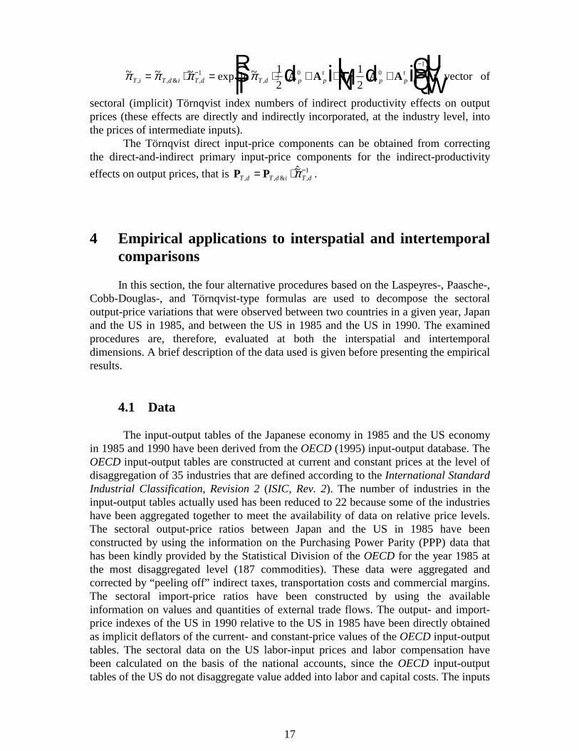
First, the four alternative index numbers of input-prices between Japan and theUS in 1985 differ widely in many industries. As shown in Figure 1, the Laspeyres,Cobb-Douglas, and Paasche indexes are particularly high, relative to the Törnqvistindex, in the goods-producing industries. The averages of the sectoral Laspeyres andPaasche indexes of direct-input prices are, respectively, 7.4 per cent higher and 7.2 percent lower than the average of sectoral Törnqvist indexes. In some cases, as forexample in Agriculture and Furniture industries, the Laspeyres index is about 15%higher than the Törnqvist index, whereas in the Food industry the Paasche index islower than 15% of the respective Törnqvist index.

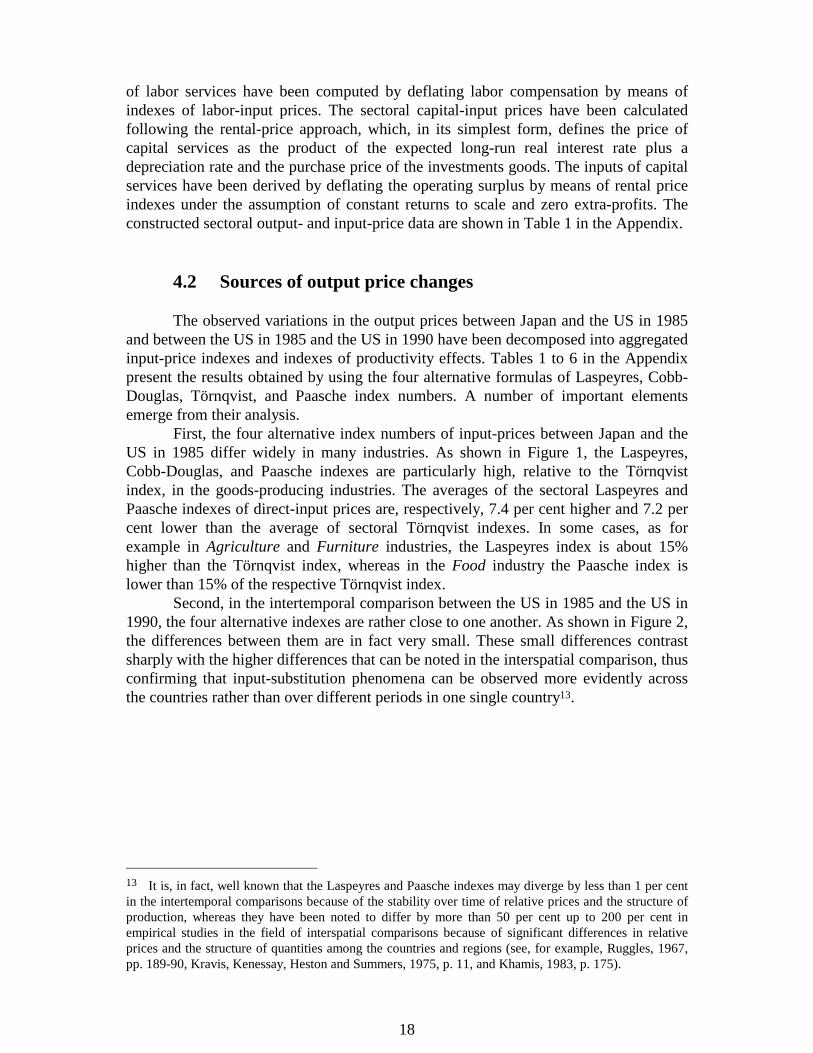
Second, in the intertemporal comparison between the US in 1985 and the US in1990, the four alternative indexes are rather close to one another. As shown in Figure 2,the differences between them are in fact very small. These small differences contrastsharply with the higher differences that can be noted in the interspatial comparison, thusconfirming that input-substitution phenomena can be observed more evidently acrossthe countries rather than over different periods in one single country13.

13 It is, in fact, well known that the Laspeyres and Paasche indexes may diverge by less than 1 per centin the intertemporal comparisons because of the stability over time of relative prices and the structure ofproduction, whereas they have been noted to differ by more than 50 per cent up to 200 per cent inempirical studies in the field of interspatial comparisons because of significant differences in relativeprices and the structure of quantities among the countries and regions (see, for example, Ruggles, 1967,pp. 189-90, Kravis, Kenessay, Heston and Summers, 1975, p. 11, and Khamis, 1983, p. 175).

19

0.8

0.85

0.9

0.95

1

1.05

1.1

1.15

1.2

Agr

icul

ture

Min

ing

Food

Tex

tile

s

Furn

itur

e

Pape

r &

Pri

nt

Che

mic

als

Non

-met

alli

c pr

.

Prim

ary

Met

al

Met

al P

rodu

cts

Mac

hine

ry

Ele

ctri

c M

ach.

Aut

omob

ile

Oth

er T

rans

p. E

q.

Prec

isio

n A

pp.

Oth

er M

anuf

.

Uti

liti

es

Con

stru

ctio

n

Tra

de &

Hot

els

Tra

nspo

rtat

ion

Fina

nce

Oth

er S

ervi

ces

Laspeyres/Törnqvist Cobb-Douglas/Törnqvist Paasche/Törnqvist

Figure 1 - Laspeyres, Cobb-Douglas, and Paasche indexes relative to Törnqvist indexes in

interspatial comparison of aggregated direct-input prices: Japan, 1985 vs. US 1985

0.986

0.988

0.99

0.992

0.994

0.996

0.998

1

1.002

1.004

Agr

icul

ture

Min

ing

Food

Tex

tile

s

Furn

itur

e

Pape

r &

Pri

nt

Che

mic

als

Non

-met

alli

c pr

.

Prim

ary

Met

al

Met

al P

rodu

cts

Mac

hine

ry

Ele

ctri

c M

ach.

Aut

omob

ile

Oth

er T

rans

p. E

q.

Prec

isio

n A

pp.

Oth

er M

anuf

.

Uti

liti

es

Con

stru

ctio

n

Tra

de &

Hot

els

Tra

nspo

rtat

ion

Fina

nce

Oth

er S

ervi

ces

Laspeyres/Törnqvist Cobb-Douglas/Törnqvist Paasche/Törnqvist

Figure 2 - Laspeyres, Cobb-Douglas, and Paasche indexes relative to Törnqvist indexes

intertemporal comparison of aggregated direct-input prices: US 1990 vs US 1985

Törnqvist indexes in

Third, in most industries, the interspatial comparison of sectoral direct-inputprices of Japan and the US in 1985 shows that the Laspeyres index is the higher boundand the Paasche index is the lower bound of the interval of values of the indexesconsidered. In some cases, however, the Cobb-Douglas input-price or quantity index

20

shows the lowest level, which lies outside the interval of values bounded by theLaspeyres and Paasche indexes. In these cases, our interpretation is that a first-orderapproximation error places the Cobb-Douglas index significantly far away from the trueunknown index number falling within the above-mentioned interval of values.

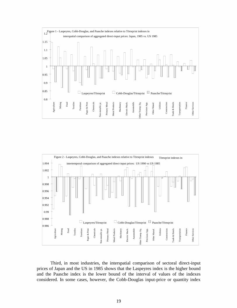
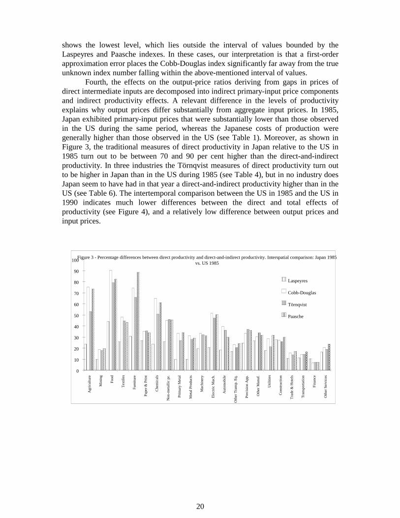
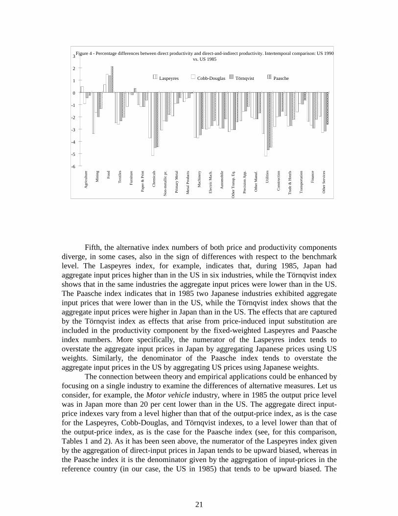
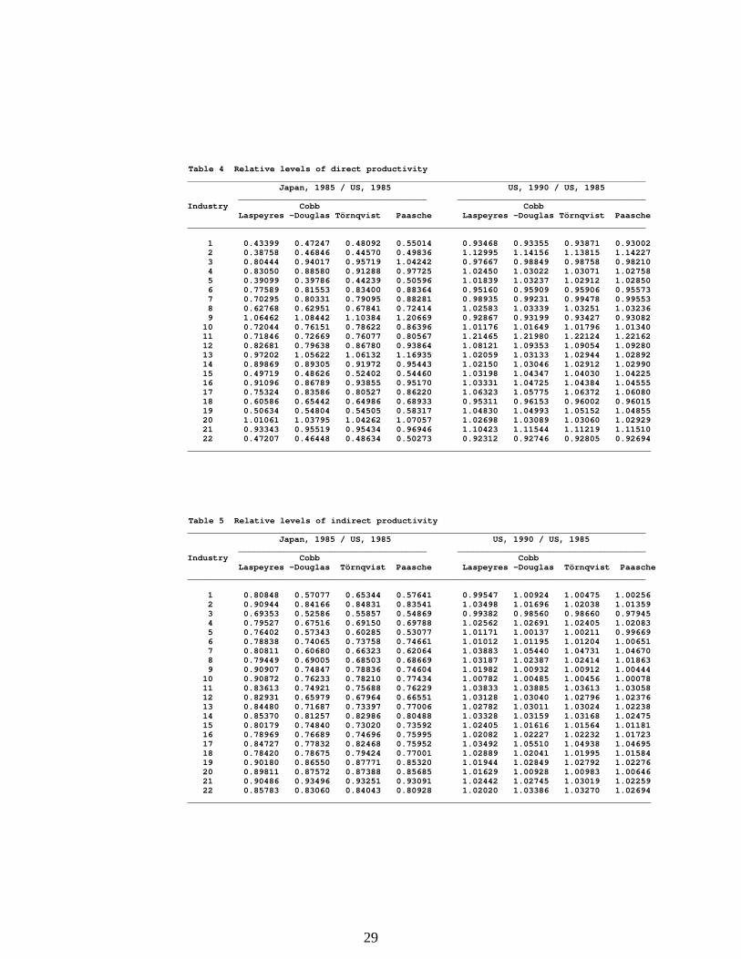
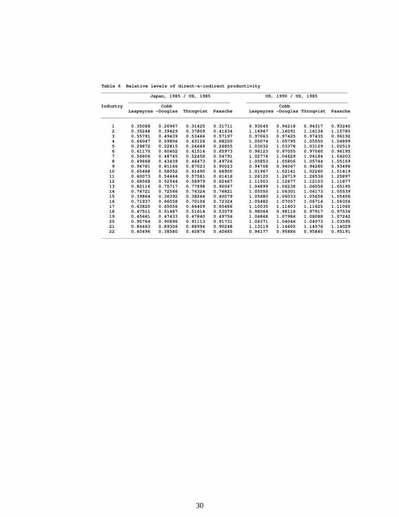
Fourth, the effects on the output-price ratios deriving from gaps in prices ofdirect intermediate inputs are decomposed into indirect primary-input price componentsand indirect productivity effects. A relevant difference in the levels of productivityexplains why output prices differ substantially from aggregate input prices. In 1985,Japan exhibited primary-input prices that were substantially lower than those observedin the US during the same period, whereas the Japanese costs of production weregenerally higher than those observed in the US (see Table 1). Moreover, as shown inFigure 3, the traditional measures of direct productivity in Japan relative to the US in1985 turn out to be between 70 and 90 per cent higher than the direct-and-indirectproductivity. In three industries the Törnqvist measures of direct productivity turn outto be higher in Japan than in the US during 1985 (see Table 4), but in no industry doesJapan seem to have had in that year a direct-and-indirect productivity higher than in theUS (see Table 6). The intertemporal comparison between the US in 1985 and the US in1990 indicates much lower differences between the direct and total effects ofproductivity (see Figure 4), and a relatively low difference between output prices andinput prices.

0

10

20

30

40

50

60

70

80

90

100

Agr

icul

ture

Min

ing

Food

Tex

tile

s

Furn

itur

e

Pape

r &

Pri

nt

Che

mic

als

Non

-met

alli

c pr

.

Prim

ary

Met

al

Met

al P

rodu

cts

Mac

hine

ry

Ele

ctri

c M

ach.

Aut

omob

ile

Oth

er T

rans

p. E

q.

Prec

isio

n A

pp.

Oth

er M

anuf

.

Uti

liti

es

Con

stru

ctio

n

Tra

de &

Hot

els

Tra

nspo

rtat

ion

Fina

nce

Oth

er S

ervi

ces

Laspeyres

Cobb-Douglas

Törnqvist

Paasche

Figure 3 - Percentage differences between direct productivity and direct-and-indirect productivity. Interspatial comparison: Japan 1985vs. US 1985

21

-6

-5

-4

-3

-2

-1

0

1

2

3

Agr

icul

ture

Min

ing

Food

Tex

tile

s

Furn

itur

e

Pape

r &

Pri

nt

Che

mic

als

Non

-met

alli

c pr

.

Prim

ary

Met

al

Met

al P

rodu

cts

Mac

hine

ry

Ele

ctri

c M

ach.

Aut

omob

ile

Oth

er T

rans

p. E

q.

Prec

isio

n A

pp.

Oth

er M

anuf

.

Uti

liti

es

Con

stru

ctio

n

Tra

de &

Hot

els

Tra

nspo

rtat

ion

Fina

nce

Oth

er S

ervi

ces

Laspeyres Cobb-Douglas Törnqvist Paasche

Figure 4 - Percentage differences between direct productivity and direct-and-indirect productivity. Intertemporal comparison: US 1990vs. US 1985

Fifth, the alternative index numbers of both price and productivity componentsdiverge, in some cases, also in the sign of differences with respect to the benchmarklevel. The Laspeyres index, for example, indicates that, during 1985, Japan hadaggregate input prices higher than in the US in six industries, while the Törnqvist indexshows that in the same industries the aggregate input prices were lower than in the US.The Paasche index indicates that in 1985 two Japanese industries exhibited aggregateinput prices that were lower than in the US, while the Törnqvist index shows that theaggregate input prices were higher in Japan than in the US. The effects that are capturedby the Törnqvist index as effects that arise from price-induced input substitution areincluded in the productivity component by the fixed-weighted Laspeyres and Paascheindex numbers. More specifically, the numerator of the Laspeyres index tends tooverstate the aggregate input prices in Japan by aggregating Japanese prices using USweights. Similarly, the denominator of the Paasche index tends to overstate theaggregate input prices in the US by aggregating US prices using Japanese weights.

The connection between theory and empirical applications could be enhanced byfocusing on a single industry to examine the differences of alternative measures. Let usconsider, for example, the Motor vehicle industry, where in 1985 the output price levelwas in Japan more than 20 per cent lower than in the US. The aggregate direct input-price indexes vary from a level higher than that of the output-price index, as is the casefor the Laspeyres, Cobb-Douglas, and Törnqvist indexes, to a level lower than that ofthe output-price index, as is the case for the Paasche index (see, for this comparison,Tables 1 and 2). As it has been seen above, the numerator of the Laspeyres index givenby the aggregation of direct-input prices in Japan tends to be upward biased, whereas inthe Paasche index it is the denominator given by the aggregation of input-prices in thereference country (in our case, the US in 1985) that tends to be upward biased. The

22

corresponding meaures of direct productivity effects vary in a symmetrical way fromthe Laspeyres index, which shows a lower level in Japan than in the US, to the Cobb-Douglas, Törnqvist and Paasche indexes showing a higher level in Japan than in the US(see Table 4). The Törnqvist and the Cobb-Douglas index numbers of direct-inputprices lie between the Laspeyres and the Paasche indexes. A different outcome can benoted by observing the index numbers of direct-and-indirect effects. As measures ofrelative levels of the aggregate input prices, both the Törnqvist and the Cobb-Douglasindexes fall outside the Laspeyres-Paasche boundaries, significantly below the level ofthe Paasche index number (see Table 3). This result arises from the system ofinterindustry relations, where the indirect productivity effects are compounded indirections that depend on the complex structure of production within the verticallyintegrated sector.

Summing up, our investigation confirms that the empirical results are sensitiveto the choice of functional forms of the index numbers, particularly when the structuraldecomposition analysis is made in the context of interspatial comparisons. Thesensitivity of results may regard, not only the magnitude, but also the sign of themeasured components. This discrepancy in the results originate, in the context of ouranalysis, from different underlying hypotheses about the technology and, in particular,price-induced input substitution phenomena.

5 Concluding remarks

In this paper, a new decomposition technique is developed by using theTörnqvist index number approach into the input-output model of prices. Thisinnovation allows us to consider a more general structure of technology than thatimplied by the usual input-output structural decomposition methods. The resultsemerging from the empirical application of this new approach are significantly differentfrom those obtained by applying the traditional procedures, particularly in theinterspatial comparisons of cases where the structure of production and relative pricesvary widely. The superiority of this approach lies in its capability to take into accountthe flexibility of current methods of production with respect to relative price changes.

The analytical procedure proposed in this paper has been presented undersimplifying strong assumptions, which can be weakened in further extensions of thiswork. The hypothesis of constant returns to scale can be relaxed following theguidelines that were established by Caves, Christensen and Diewert (1982), whosuggest to include the possibility of decreasing and increasing returns to scale and non-zero extra-profits due to the rewards to scale factors. Furthermore, more general indexnumbers can be introduced into the input-output system. A promising example is givenby Diewert's (1976, pp. 130-31) “Quadratic mean of order r quantity and priceindexes”, which include, as special cases, the four index numbers considered here. TheQuadratic mean of order r indexes are, however, strongly non-linear. Still, they can beintegrated into the input-output equation system to account for the direct-and-indirectinput requirements by using iterative solution algorithms. Finally, in the light oftraditional input-output structural decomposition analyses, procedures that are parallel

23

to those based on index numbers can be developed by referring to output-pricedifferences rather than output-price ratios.

References

Allen, R.G.D. (1949), The Economic Theory of Index Numbers, Economica, N.S., 16, 197-203.

Blackorby, C., W.E. Schworm, and T.C.G. Fisher (1986), Testing for the Existence of Input Aggregates in an Economy Production Function, University of British Columbia, Department of Economics, Discussion paper 86-26, Vancouver, BC, Canada.

Caves, D.W., L.R. Christensen, and W.E. Diewert (1982), The Economic Theory of Index Numbers and the Measurement of Input, Output, and Productivity, Econometrica, 50, 1393-1414.

Denny, M. and M. Fuss (1983a), A General Approach to International and Interspatial Productivity Comparisons, Journal of Econometrics, 23, 315-30.

Denny, M. and M. Fuss (1983b), The Use of Discrete Variables in Superlative Index Number Comparisons, International Economic Review, 24, 419-21.

Dietzenbacher, E. (1999), An Intercountry Decomposition of Output Growth in EC Countries, in this book.

Dietzenbacher, E. and Los, B. (1997), Analyzing Decomposition Analyses, in András Simonovits and Albert E. Steenge (eds.), Prices, Growth and Cycles(Macmillan, London), pp. 108-131.

Dietzenbacher, E. and Los, B. (1998), Structural Decomposition Techniques: Sense and Sensitivity, Economic Systems Research, 10,

Diewert, W.E. (1976), Exact and Superlative Index Numbers, Journal ofEconometrics, 4, 115-45.

Diewert, W.E. (1981), The Economic Theory of Index Numbers: A Survey, in A. Deaton (ed. by), Essays in the Theory and Measurement of Consumer Behavior in Honor of Sir Richard Stone (Cambridge University Press, Cambridge), pp. 163-208.

24

Diewert, W.E. (1987), Index numbers, in J. Eatwell, M. Milgate, and P. Newman (eds.), The New Palgrave: A Dictionary of Economics (Heidelberg, Physica-Verlag), pp. 67-86.

Diewert, W.E. (1998), Index Number Theory Using Differences Rather Than Ratios,University of British Columbia, Department of Economics, Discussion paperNo. 98-10, Vancouver, BC, Canada.

Fisher, F. M. (1988), Production-Theoretic Input Price Indices and the Measurement of Real Aggregate Input Use, in W. Eichhorn (ed. by), Measurement in Economics (Heidelberg, Physica-Verlag), pp. 87-98.

Frisch, R. (1936), Annual Survey of General Economic Theory: The Problem of Index Numbers, Econometrica, 4, 1-39.

Fromm, G. (1968), Comment on B.N.Vaccara and N.W. Simon, 'Factors Affecting the Postwar Industrial Composition of Real Product ', in J. W. Kendrick (ed. by), The Industrial Composition of Income and Product, National Bureau of Economic Research, Studies in Income and Wealth, Volume 32, (Columbia

University Press, New York), pp. 59-66.

Fujikawa, K.; H. Izumi; and C. Milana (1995a), Multilateral Comparison of Cost Structure in the Input-Output Tables of Japan, the US and West Germany, Economic Systems Research, 7, 321-42.

Fujikawa, K.; H. Izumi; and C. Milana (1995b), A Comparison of Cost Structures in Japan and the US Using Input-Output Tables, Journal of Applied Input-Output Analysis, 2, 1-23.

Hulten, C. R. (1978), Growth Accounting with Intermediate Inputs, Review ofEconomic Studies, 45, 511-18.

Jorgenson, D.W., M. Kuroda, and M. Nishimizu (1987), Japan-US Industry Level Productivity Comparisons, 1960-1979, Journal of the Japanese International Economies, 1, 1-30.

Jorgenson, D.W. and M. Kuroda (1990), Productivity and International Competitiveness in Japan and the United States, 1960-1985 . In C.R. Hulten (ed. by), Productivity Growth in Japan and the United States, NBER, Studies in Income and Wealth 53 (The University of Chicago Press, Chicago), pp. 29-57.

Jorgenson, D.W. and M. Nishimizu (1978), U.S. and Japanese Economic Growth, 1952-1974: An International Comparison, Economic Journal, 88, 707-26.

Karasz, P. (1992), Influence of Interindustrial Relationships on Prices in Czechoslovakia, Economic Systems Research, 4, 377-84.

25

Khamis, S. H. (1983), Application of Index Numbers in International Comparisons and Related Concepts, in International Statistical Institute, Proceedings of the 44th Session, Bulletin of the International Statistical Institute, Madrid, 12-22 September 1983, Vol. L, Book 1, pp. 171-88.

Klein, L.R. (1952-53), On the Interpretation of Professor Leontief's System, Review of Economic Studies, 20, 131-36.

Klein, L.R. (1956), The Interpretation of Leontief's System: A Reply, Review of Economic Studies, 24, 69-70.

Kravis, I. B., Z. Kenessy, A. Heston, R. Summers (1975), A System of International Comparisons of Gross Product and Purchasing Power (John Hopkins University, Baltimore).

Leontief, W. (1936), Quantitative Input-Output Relations in the Economic System of the United States, Review of Economics and Statistics, 18, 105-25.

Leontief, W. (1941), The Structure of the American Economy, 1919-1929 (Oxford University Press, New York) (2nd edition, revised and enlarged, 1951).

Morishima, M. (1956), A Comment on Dr. Klein's Interpretation of Leontief's System, Review of Economic Studies, 24, 65-68.

Morishima, M. (1957), Dr. Klein's Interpretation of Leontief's System: A Rejoinder, Review of Economic Studies, 25, 59-61.

Muellbauer, J.N.J. (1972), The Theory of True Input Price Indices, University of Warwick, Economic Research Paper 17, Coventry, United Kingdom.

OECD (1995), The OECD Input-Output Database, Paris.

Pasinetti, L. L. (1973), The Notion of Vertical Integration in Economic Analysis, Metroeconomica, 25, 1-29.

Rose, A. and Casler, S. (1996), Input-Output Structural Decomposition Analysis: A Critical Appraisal, Economic Systems Research, 8, 33-62.

Rose, A. and C.Y. Chen (1991), Sources of Change in Energy Use in the U.S. Economy, 1972-1982, Resources and Energy,13, 1-21.

Ruggles, R. (1967), Price Indexes and International Price Comparisons, in W. Fellner (ed. by), Ten Economic Studies in the Tradition of Irving Fisher, John Wiley, New York, pp. 171-205.

26

Samuelson, P.A. and S. Swamy (1974), Invariant Economic Index Numbers and Canonical Duality: Survey and Synthesis, American Economic Review, 64, 566-93.

Skolka, J. (1989), Input-Output Structural Decomposition Analysis for Austria, Journal of Policy Modeling, 11, 45-66.

Vaccara, B. N. and N. W. Simon (1968), Factors Affecting the Postwar Industrial Composition of Real Product, in J. W. Kendrick (ed. by), The Industrial Composition of Income and Product, National Bureau of Economic Research, Studies in Income and Wealth, Volume 32 (Columbia University Press, New

York), pp. 19-58.

27

APPENDIX

Table 1 Sectoral output- and primary-input price indexes in Japan (1985) and the US (1985 and 1990)

_______________________________________________________________________________________________________________ ISIC, Rev.2 Output prices, US 1985=1.0 | Import prices, US 1985=1.0 Industry classification _____________________________|________________________________ code Japan,1985 US,1985 US,1990 | Japan,1985 US,1985 US,1990 _______________________________________________________________________________________________________________

1 Agriculture, forestry & f. 1 2.40882 1.0 1.27335 1.35220 1.0 1.27395 2 Mining and quarrying 2 2.17490 1.0 0.98376 1.29372 1.0 0.79565 3 Food, beverages & tobacco 31 1.37377 1.0 1.20852 1.09344 1.0 1.21840 4 Textiles, apparel & leath. 32 1.02708 1.0 1.10933 1.00677 1.0 1.09765 5 Wood products & furniture 33 2.30863 1.0 1.13847 1.32715 1.0 1.13285 6 Paper and printing 34 1.18806 1.0 1.23280 1.04701 1.0 1.26660 7 Chemicals and medicines 35 1.50457 1.0 1.08994 1.12614 1.0 1.04958 8 Non-metallic mineral prod. 36 1.44295 1.0 1.09525 1.11073 1.0 1.09452 9 Primary metal products 37 0.84619 1.0 1.21430 1.00965 1.0 1.20707 10 Metal products 381 1.00905 1.0 1.15012 1.00226 1.0 1.13096 11 Machinery 382 1.15578 1.0 0.92076 1.03894 1.0 0.96855 12 Electric apparatus, n.e.c. 383 0.94408 1.0 1.03734 0.98601 1.0 0.98075 13 Motor vehicles 3843 0.79609 1.0 1.09862 0.94902 1.0 1.10170 14 Other transp. equipment 384-3843 0.97384 1.0 1.10932 1.00754 1.0 1.08312 15 Professional goods 385 1.70705 1.0 1.10021 1.17676 1.0 1.05744 16 Other manufacturing 39 1.04888 1.0 1.11678 1.01222 1.0 1.11559 17 Electricity, gas & water 4 1.54188 1.0 1.05232 1.13547 1.0 1.05816 18 Construction 5 1.63117 1.0 1.18344 - - - 19 Trade, restaurants & hotels 6 1.72969 1.0 1.13361 1.18242 1.0 1.11621 20 Transportation & communicat. 7 0.91264 1.0 1.11375 1.00023 1.0 1.05535 21 Finance and business serv. 8 1.15117 1.0 1.08451 1.03779 1.0 1.22700 22 Other services 9 1.96613 1.0 1.29522 1.24153 1.0 1.23460 _______________________________________________________________________________________________________________

Table 1 (continued)_______________________________________________________________________________________________________________

ISIC, Rev.2 Labor-input prices |Capital-input prices Industry classification ______________________________|____________________________ code Japan,1985 US,1985 US,1990 |Japan,1985 US,1985 US,1990

_______________________________________________________________________________________________________________

1 Agriculture, forestry & f. 1 0.37000 1.0 1.25190 1.10158 1.0 1.16337 2 Mining and quarrying 2 0.52706 1.0 1.18899 1.06967 1.0 1.12945 3 Food, beverages & tobacco 31 0.39313 1.0 1.19586 1.10134 1.0 1.16865 4 Textiles, apparel & leath. 32 0.42300 1.0 1.24210 1.03776 1.0 1.09542 5 Wood products & furniture 33 0.37592 1.0 1.20553 1.06978 1.0 1.12939 6 Paper and printing 34 0.50781 1.0 1.23155 1.10132 1.0 1.16486 7 Chemicals and medicines 35 0.41982 1.0 1.22379 1.05609 1.0 1.13848 8 Non-metallic mineral prod. 36 0.40602 1.0 1.19622 1.07001 1.0 1.12943 9 Primary metal products 37 0.46311 1.0 1.17922 1.07020 1.0 1.13001 10 Metal products 381 0.39827 1.0 1.21056 1.07100 1.0 1.13024 11 Machinery 382 0.43319 1.0 1.20995 1.06942 1.0 1.12975 12 Electric apparatus, n.e.c. 383 0.34821 1.0 1.21024 0.99703 1.0 1.12287 13 Motor vehicles 3843 0.34671 1.0 1.21134 1.04587 1.0 1.14800 14 Other transp. equipment 384-3843 0.57593 1.0 1.20998 1.04254 1.0 1.14757 15 Professional goods 385 0.46272 1.0 1.21003 1.01061 1.0 1.11359 16 Other manufacturing 39 0.50862 1.0 1.25598 1.07002 1.0 1.13002 17 Electricity, gas & water 4 0.84766 1.0 1.22211 1.06896 1.0 1.18340 18 Construction 5 0.68875 1.0 1.22930 1.03776 1.0 1.09542 19 Trade, restaurants & hotels 6 0.63930 1.0 1.21394 1.18889 1.0 1.24946 20 Transportation & communicat. 7 0.78264 1.0 1.16316 0.86513 1.0 1.16377 21 Finance and business serv. 8 0.82366 1.0 1.25413 1.13742 1.0 1.24065 22 Other services 9 0.60843 1.0 1.26375 1.15738 1.0 1.22125 _______________________________________________________________________________________________________________

28

Table 2 Indexes of aggregate direct-input prices __________________________________________________________________________________________ Japan, 1985 / US, 1985 US, 1990 / US, 1985 _____________________________________ _____________________________________ Industry Cobb Cobb Laspeyres -Douglas Törnqvist Paasche Laspeyres -Douglas Törnqvist Paasche __________________________________________________________________________________________

1 1.32519 1.13809 1.15846 1.04541 1.18424 1.18874 1.19530 1.19018 2 1.08389 1.01885 0.96935 0.84295 1.12372 1.12302 1.11967 1.11160 3 1.43205 1.29157 1.31495 1.10512 1.18689 1.19460 1.19351 1.18033 4 1.00371 0.90979 0.93761 0.85299 1.13993 1.14286 1.14340 1.13650 5 1.16808 0.91851 1.02131 0.90264 1.17092 1.17532 1.17163 1.15941 6 1.04981 0.96890 0.99084 0.92181 1.17822 1.18236 1.18232 1.17313 7 1.32824 1.20862 1.19003 1.05764 1.08507 1.08156 1.08425 1.07833 8 1.04489 0.90835 0.97890 0.90570 1.13069 1.13182 1.13086 1.12354 9 1.02108 0.91763 0.93406 0.90087 1.13030 1.13171 1.13449 1.12769 10 0.87178 0.76840 0.79333 0.72696 1.16554 1.16908 1.17078 1.16365 11 0.93118 0.83989 0.87928 0.83038 1.12482 1.12314 1.12447 1.11840 12 0.88614 0.75184 0.81926 0.78057 1.13361 1.13436 1.13126 1.12158 13 0.93091 0.84084 0.84491 0.77381 1.13039 1.13304 1.13096 1.12124 14 0.92947 0.86968 0.89566 0.87518 1.14249 1.14311 1.14162 1.13317 15 0.92967 0.83007 0.89453 0.84872 1.14669 1.14803 1.14455 1.13539 16 0.99822 0.91032 0.98442 0.95549 1.16765 1.16955 1.16574 1.15398 17 1.32941 1.28879 1.24164 1.16141 1.11630 1.11310 1.11937 1.11886 18 1.12442 1.06747 1.06003 0.98826 1.13628 1.13792 1.13613 1.12795 19 1.00870 0.94793 0.94276 0.87580 1.18865 1.19021 1.19201 1.18836 20 0.97704 0.94727 0.95153 0.92232 1.14637 1.14816 1.14783 1.14380 21 1.11601 1.09958 1.09861 1.07454 1.20933 1.20970 1.20618 1.19755 22 0.98843 0.91323 0.95621 0.92814 1.20059 1.20127 1.20203 1.19564 __________________________________________________________________________________________

Table 3 Indexes of aggregate direct-&-indirect primary-input prices __________________________________________________________________________________________ Japan, 1985 / US, 1985 US, 1990 / US, 1985 _____________________________________ _____________________________________ Industry Cobb Cobb Laspeyres -Douglas Törnqvist Paasche Laspeyres -Douglas Törnqvist Paasche __________________________________________________________________________________________

1 0.76385 0.64959 0.75698 0.84520 1.18728 1.19972 1.20098 1.18478 2 0.90549 0.85753 0.82231 0.76661 1.13900 1.14206 1.14248 1.15048 3 0.78576 0.67918 0.73450 0.76643 1.16250 1.17741 1.17752 1.17303 4 0.70047 0.61425 0.64835 0.67836 1.16367 1.17361 1.17089 1.16562 5 0.61999 0.52671 0.61569 0.68964 1.16704 1.17693 1.17410 1.17299 6 0.78380 0.71761 0.73082 0.72673 1.18589 1.19649 1.19655 1.18500 7 0.82436 0.73339 0.78926 0.85469 1.13575 1.14039 1.13554 1.12020 8 0.71752 0.62681 0.67057 0.71957 1.15176 1.15884 1.15816 1.15935 9 0.76177 0.68682 0.73638 0.81895 1.13532 1.14226 1.14484 1.15004 10 0.67506 0.58578 0.62046 0.66061 1.16644 1.17475 1.17612 1.17275 11 0.70983 0.62926 0.66551 0.69431 1.15921 1.16678 1.16509 1.16126 12 0.58974 0.49606 0.55680 0.64733 1.16055 1.16884 1.16289 1.15667 13 0.71686 0.60278 0.62014 0.65372 1.15569 1.16715 1.16516 1.15244 14 0.74811 0.70668 0.74327 0.74714 1.17076 1.17922 1.17779 1.17088 15 0.68416 0.62123 0.65319 0.68049 1.16023 1.16658 1.16246 1.16270 16 0.75859 0.69811 0.73533 0.75454 1.18777 1.19559 1.19176 1.17800 17 1.00971 1.00309 1.02395 0.98403 1.16871 1.17442 1.17465 1.15792 18 0.86581 0.83983 0.84192 0.77499 1.15428 1.16114 1.15879 1.16053 19 0.86062 0.82044 0.82747 0.78979 1.21571 1.22411 1.22529 1.21147 20 0.83717 0.82954 0.83152 0.82834 1.15378 1.15882 1.15911 1.16244 21 1.03891 1.02806 1.02447 0.97231 1.23665 1.24291 1.24259 1.22678 22 0.79991 0.75853 0.80363 0.79619 1.23293 1.24194 1.24134 1.21980 __________________________________________________________________________________________

29

Table 4 Relative levels of direct productivity __________________________________________________________________________________________ Japan, 1985 / US, 1985 US, 1990 / US, 1985 _____________________________________ _____________________________________ Industry Cobb Cobb Laspeyres -Douglas Törnqvist Paasche Laspeyres -Douglas Törnqvist Paasche __________________________________________________________________________________________

1 0.43399 0.47247 0.48092 0.55014 0.93468 0.93355 0.93871 0.93002 2 0.38758 0.46846 0.44570 0.49836 1.12995 1.14156 1.13815 1.14227 3 0.80444 0.94017 0.95719 1.04242 0.97667 0.98849 0.98758 0.98210 4 0.83050 0.88580 0.91288 0.97725 1.02450 1.03022 1.03071 1.02758 5 0.39099 0.39786 0.44239 0.50596 1.01839 1.03237 1.02912 1.02850 6 0.77589 0.81553 0.83400 0.88364 0.95160 0.95909 0.95906 0.95573 7 0.70295 0.80331 0.79095 0.88281 0.98935 0.99231 0.99478 0.99553 8 0.62768 0.62951 0.67841 0.72414 1.02583 1.03339 1.03251 1.03236 9 1.06462 1.08442 1.10384 1.20669 0.92867 0.93199 0.93427 0.93082 10 0.72044 0.76151 0.78622 0.86396 1.01176 1.01649 1.01796 1.01340 11 0.71846 0.72669 0.76077 0.80567 1.21465 1.21980 1.22124 1.22162 12 0.82681 0.79638 0.86780 0.93864 1.08121 1.09353 1.09054 1.09280 13 0.97202 1.05622 1.06132 1.16935 1.02059 1.03133 1.02944 1.02892 14 0.89869 0.89305 0.91972 0.95443 1.02150 1.03046 1.02912 1.02990 15 0.49719 0.48626 0.52402 0.54460 1.03198 1.04347 1.04030 1.04225 16 0.91096 0.86789 0.93855 0.95170 1.03331 1.04725 1.04384 1.04555 17 0.75324 0.83586 0.80527 0.86220 1.06323 1.05775 1.06372 1.06080 18 0.60586 0.65442 0.64986 0.68933 0.95311 0.96153 0.96002 0.96015 19 0.50634 0.54804 0.54505 0.58317 1.04830 1.04993 1.05152 1.04855 20 1.01061 1.03795 1.04262 1.07057 1.02698 1.03089 1.03060 1.02929 21 0.93343 0.95519 0.95434 0.96946 1.10423 1.11544 1.11219 1.11510 22 0.47207 0.46448 0.48634 0.50273 0.92312 0.92746 0.92805 0.92694 ___________________________________________________________________________________________

Table 5 Relative levels of indirect productivity __________________________________________________________________________________________ Japan, 1985 / US, 1985 US, 1990 / US, 1985 _____________________________________ _____________________________________ Industry Cobb Cobb Laspeyres -Douglas Törnqvist Paasche Laspeyres -Douglas Törnqvist Paasche __________________________________________________________________________________________

1 0.80848 0.57077 0.65344 0.57641 0.99547 1.00924 1.00475 1.00256 2 0.90944 0.84166 0.84831 0.83541 1.03498 1.01696 1.02038 1.01359 3 0.69353 0.52586 0.55857 0.54869 0.99382 0.98560 0.98660 0.97945 4 0.79527 0.67516 0.69150 0.69788 1.02562 1.02691 1.02405 1.02083 5 0.76402 0.57343 0.60285 0.53077 1.01171 1.00137 1.00211 0.99669 6 0.78838 0.74065 0.73758 0.74661 1.01012 1.01195 1.01204 1.00651 7 0.80811 0.60680 0.66323 0.62064 1.03883 1.05440 1.04731 1.04670 8 0.79449 0.69005 0.68503 0.68669 1.03187 1.02387 1.02414 1.01863 9 0.90907 0.74847 0.78836 0.74604 1.01982 1.00932 1.00912 1.00444 10 0.90872 0.76233 0.78210 0.77434 1.00782 1.00485 1.00456 1.00078 11 0.83613 0.74921 0.75688 0.76229 1.03833 1.03885 1.03613 1.03058 12 0.82931 0.65979 0.67964 0.66551 1.03128 1.03040 1.02796 1.02376 13 0.84480 0.71687 0.73397 0.77006 1.02782 1.03011 1.03024 1.02238 14 0.85370 0.81257 0.82986 0.80488 1.03328 1.03159 1.03168 1.02475 15 0.80179 0.74840 0.73020 0.73592 1.02405 1.01616 1.01564 1.01181 16 0.78969 0.76689 0.74696 0.75995 1.02082 1.02227 1.02232 1.01723 17 0.84727 0.77832 0.82468 0.75952 1.03492 1.05510 1.04938 1.04695 18 0.78420 0.78675 0.79424 0.77001 1.02889 1.02041 1.01995 1.01584 19 0.90180 0.86550 0.87771 0.85320 1.01944 1.02849 1.02792 1.02276 20 0.89811 0.87572 0.87388 0.85685 1.01629 1.00928 1.00983 1.00646 21 0.90486 0.93496 0.93251 0.93091 1.02442 1.02745 1.03019 1.02259 22 0.85783 0.83060 0.84043 0.80928 1.02020 1.03386 1.03270 1.02694 ___________________________________________________________________________________________

30

Table 6 Relative levels of direct-&-indirect productivity __________________________________________________________________________________________ Japan, 1985 / US, 1985 US, 1990 / US, 1985 _____________________________________ _____________________________________ Industry Cobb Cobb Laspeyres -Douglas Törnqvist Paasche Laspeyres -Douglas Törnqvist Paasche __________________________________________________________________________________________

1 0.35088 0.26967 0.31425 0.31711 0.93045 0.94218 0.94317 0.93240 2 0.35248 0.39429 0.37809 0.41634 1.16947 1.16091 1.16134 1.15780 3 0.55791 0.49439 0.53466 0.57197 0.97063 0.97425 0.97435 0.96192 4 0.66047 0.59806 0.63126 0.68200 1.05074 1.05795 1.05550 1.04899 5 0.29872 0.22815 0.26669 0.26855 1.03032 1.03378 1.03129 1.02510 6 0.61170 0.60402 0.61514 0.65973 0.96123 0.97055 0.97060 0.96195 7 0.56806 0.48745 0.52458 0.54791 1.02776 1.04629 1.04184 1.04203 8 0.49868 0.43439 0.46473 0.49726 1.05853 1.05806 1.05744 1.05159 9 0.96781 0.81166 0.87023 0.90023 0.94708 0.94067 0.94280 0.93496 10 0.65468 0.58052 0.61490 0.66900 1.01967 1.02141 1.02260 1.01419 11 0.60073 0.54444 0.57581 0.61416 1.26120 1.26719 1.26536 1.25897 12 0.68568 0.52544 0.58979 0.62467 1.11503 1.12677 1.12103 1.11877 13 0.82116 0.75717 0.77898 0.90047 1.04899 1.06238 1.06056 1.05195 14 0.76721 0.72566 0.76324 0.76821 1.05550 1.06301 1.06173 1.05539 15 0.39864 0.36392 0.38264 0.40079 1.05680 1.06033 1.05658 1.05456 16 0.71937 0.66558 0.70106 0.72324 1.05482 1.07057 1.06714 1.06356 17 0.63820 0.65056 0.66409 0.65486 1.10035 1.11603 1.11625 1.11060 18 0.47511 0.51487 0.51614 0.53079 0.98064 0.98116 0.97917 0.97536 19 0.45661 0.47433 0.47840 0.49756 1.06868 1.07984 1.08088 1.07242 20 0.90764 0.90896 0.91113 0.91731 1.04371 1.04046 1.04073 1.03595 21 0.84463 0.89306 0.88994 0.90248 1.13119 1.14605 1.14576 1.14029 22 0.40496 0.38580 0.40874 0.40685 0.94177 0.95886 0.95840 0.95191 __________________________________________________________________________________________