the intended and unintended effects of u.s. agricultural
TRANSCRIPT
This PDF is a selection from a published volume from the National Bureau of Economic Research
Volume Title: The Intended and Unintended Effects of U.S. Agricultural and Biotechnology Policies
Volume Author/Editor: Joshua S. Graff Zivin and Jeffrey M. Perloff,editors
Volume Publisher: University of Chicago Press
Volume ISBN: 0-226-98803-1; 978-0-226-98803-0 (cloth)
Volume URL: http://www.nber.org/books/perl10-1
Conference Date: March 4-5, 2010
Publication Date: February 2012
Chapter Title: Commodity Price Volatility in the Biofuel Era: An Examination of the Linkage between Energy and Agricultural Markets
Chapter Authors: Thomas W. Hertel, Jayson Beckman
Chapter URL: http://www.nber.org/chapters/c12113
Chapter pages in book: (p. 189 - 221)
189
6.1 Introduction
U.S. policymakers have responded to increased public interest in reduc-ing greenhouse gas (GHG) emissions and lessening dependence on foreign supplies of energy with a Renewable Fuels Standard (RFS) that imposes aggressive mandates on biofuel use in domestic refi ning. These mandates are in addition to the longstanding price policies (blending subsidies and import tariffs) used to promote the domestic ethanol industry’s growth. Recently, a number of authors have begun to explore the linkages between energy and agricultural markets in light of these new policies (McPhail and Babock 2008; Hochman, Sexton, and Zilberman 2008; Gohin and Chantret 2010; Tyner 2009). It is clear from this work that we are entering a new era in which energy prices will play a more important role in driving agricultural commodity prices. However, based on experience during the past year, it is also clear that the coordination between energy and agricultural markets is fundamentally different at high oil prices versus low oil prices, as well as in the presence of binding policy regimes.
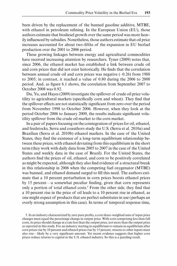
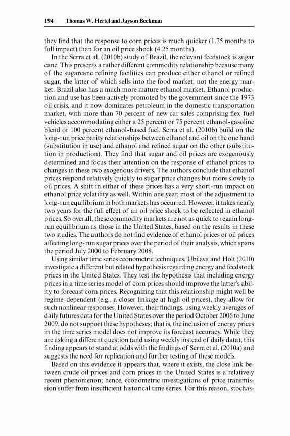
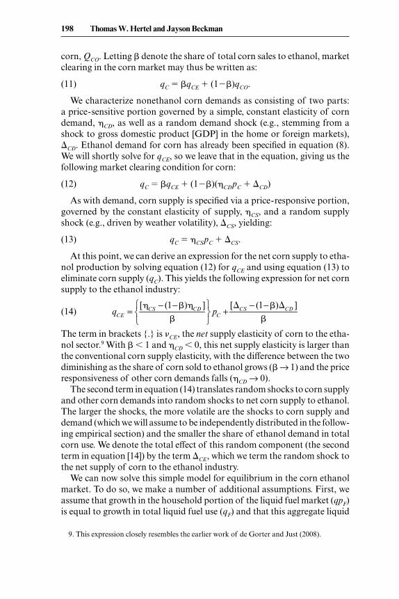
Figure 6.1 illustrates how the linkage between energy and corn prices has
6Commodity Price Volatility in the Biofuel EraAn Examination of the Linkage between Energy and Agricultural Markets
Thomas W. Hertel and Jayson Beckman
Thomas W. Hertel is Distinguished Professor of Agricultural Economics, adjunct profes-sor of economics, and executive director of the Center for Global Trade Analysis Project at Purdue University. Jayson Beckman is an economist at the Economic Research Service of the U.S. Department of Agriculture.
The authors thank Wally Tyner for valuable discussions on this topic. V. Kerry Smith served as our National Bureau of Economic Research (NBER) discussant; he and members of the NBER workshop, as well as two anonymous reviewers, provided useful comments on this chapter. The views expressed are those of the authors and do not necessarily refl ect those of the Economic Research Service (ERS) or the U.S. Department of Agriculture (USDA).

190 Thomas W. Hertel and Jayson Beckman
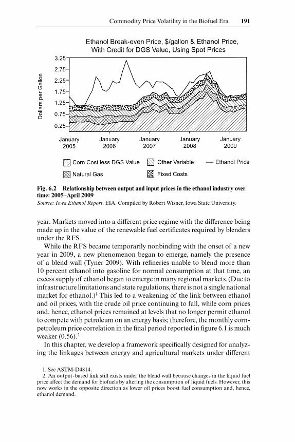
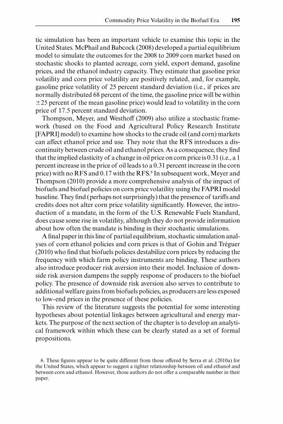
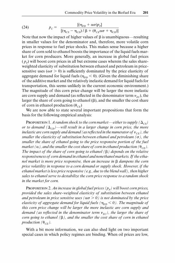
varied over the 2001 to 2009 period. With oil prices below $75 a barrel from January 2001 to August 2007, the correlation between monthly oil and corn prices was just 0.32. During much of this period, the share of corn produc-tion going to ethanol was still modest, and ethanol capacity was still being constructed. Also, considerable excess profi ts appear to have been available to the industry over this period (fi gure 6.2)—a phenomenon that loosened any potential link between ethanol prices on the one hand and corn prices on the other. Indeed, Tyner (2009) reports a – 0.08 correlation between ethanol and corn prices in the period 1988 to 2005. The year 2006 was a key turning point in the ethanol market, as this was when methyl tertiary butyl ether (MTBE) was banned as an additive and ethanol took over the entire market for oxygenator/ octane enhancers in gasoline. In this use, the demand for ethanol was not very price- responsive and ethanol was priced at a premium when converted to an energy equivalent basis.
When oil prices reached and remained above $75 a barrel from Sep-tember 2007 to October 2008, the correlation between crude oil and corn became much stronger (0.92, see fi gure 6.1 again), with per bushel corn prices remaining consistently at about 5 percent of crude oil prices per bar-rel. In this price range, the 2008 RFS appeared to be nonbinding. However, as oil prices subsequently fell, many ethanol plants were mothballed, and the RFS became binding at year’s end in 2008. That is to say, without this mandate, even less ethanol would have been produced in December of that
Fig. 6.1 Monthly oil (Cushing, OK Spot Price $/ barrel) and corn (Central Illinois no. 2 Yellow $/ bushel) prices, January 2001 to May 2009
Commodity Price Volatility in the Biofuel Era 191
year. Markets moved into a different price regime with the difference being made up in the value of the renewable fuel certifi cates required by blenders under the RFS.
While the RFS became temporarily nonbinding with the onset of a new year in 2009, a new phenomenon began to emerge, namely the presence of a blend wall (Tyner 2009). With refi neries unable to blend more than 10 percent ethanol into gasoline for normal consumption at that time, an excess supply of ethanol began to emerge in many regional markets. (Due to infrastructure limitations and state regulations, there is not a single national market for ethanol.)1 This led to a weakening of the link between ethanol and oil prices, with the crude oil price continuing to fall, while corn prices and, hence, ethanol prices remained at levels that no longer permit ethanol to compete with petroleum on an energy basis; therefore, the monthly corn- petroleum price correlation in the fi nal period reported in fi gure 6.1 is much weaker (0.56).2
In this chapter, we develop a framework specifi cally designed for analyz-ing the linkages between energy and agricultural markets under different
Fig. 6.2 Relationship between output and input prices in the ethanol industry over time: 2005– April 2009Source: Iowa Ethanol Report, EIA. Compiled by Robert Wisner, Iowa State University.
1. See ASTM- D4814.2. An output- based link still exists under the blend wall because changes in the liquid fuel
price affect the demand for biofuels by altering the consumption of liquid fuels. However, this now works in the opposite direction as lower oil prices boost fuel consumption and, hence, ethanol demand.

192 Thomas W. Hertel and Jayson Beckman
policy regimes.3 We employ a combination of theoretical analysis, econo-metrics, and stochastic simulation. Specifi cally, we are interested in examin-ing how energy price volatility has been transmitted to commodity prices and how changes in energy policy regimes affect the inherent volatility of agricultural commodity prices in response to traditional supply- side shocks. We fi nd that biofuels have played an important role in facilitating increased integration between energy and agricultural markets. In the absence of a binding RFS, and assuming that the blend wall is relaxed by expanding the maximum permissible ethanol content in petroleum as has recently been the case, we fi nd that, by 2015, the contribution of energy price volatility to year- on- year corn price variation will be much greater—amounting to nearly two- thirds of the crop supply- induced volatility. However, if the RFS is binding in 2015, then the role of energy price volatility in crop price vola-tility is diminished. Meanwhile, the sensitivity of crop prices to traditional supply- side shocks is exacerbated due to the price inelastic nature of RFS demands. Indeed, the presence of a totally inelastic demand for corn in ethanol—stemming from the combination of a blend wall and a RFS both set in the range of fi fteen billion gallons per year—would boost the sensitiv-ity of corn prices to supply- side shocks by more than 50 percent.
6.2 Literature Review
Energy and energy intensive inputs play a large role in the production of agricultural products. Gellings and Parmenter (2004) estimate that energy accounts for 70 to 80 percent of the total costs used to manufacture fer-tilizers, which, in turn, represent a large component of corn production costs. Additional linkages come in the form of transportation of inputs and the fi nal output as well as the use of diesel or gasoline on- farm. Over-all, USDA/ ERS Cost of Production estimates indicate that energy inputs accounted for almost 30 percent of the total cost of corn production for the United States in 2008.4
Another important linkage to energy markets is on the output side as agricultural commodities are increasingly being used as feedstocks for liq-uid biofuels. Hertel, Tyner, and Birur (2010) estimate that higher oil prices accounted for about two- thirds of the growth in U.S. ethanol output over the 2001 to 2006 period. The remainder of this growth is estimated to have
3. We ignore the nonmarket impacts of biofuels, which are important and have commanded much of the public’s attention—particularly since the publication of Searchinger et al. (2008). Carbone and Smith (2008) point out how the presence of such considerations can introduce interactions that alter the market and welfare impacts of environmental policies.
4. Comparing the USDA numbers across time regimes further strengthens our argument that the link between energy and agricultural commodities has increased over time. From 1996 to 2000, the average share of energy inputs (fertilizer and fuel, lube, and electricity) in total corn producer costs was 19.6 percent. From 2001 to 2004, this average share was 20.9 percent. But for 2007 to 2008, the share increased to 31.5 percent.
Commodity Price Volatility in the Biofuel Era 193
been driven by the replacement of the banned gasoline additive, MTBE, with ethanol in petroleum refi ning. In the European Union (EU), those authors estimate that biodiesel growth over the same period was more heav-ily infl uenced by subsidies. Nonetheless, those authors estimate that oil price increases accounted for about two- fi fths of the expansion in EU biofuel production over the 2001 to 2006 period.
These growing linkages between energy and agricultural commodities have received increasing attention by researchers. Tyner (2009) notes that, since 2006, the ethanol market has established a link between crude oil and corn prices that did not exist historically. He fi nds that the correlation between annual crude oil and corn prices was negative (– 0.26) from 1988 to 2005; in contrast, it reached a value of 0.80 during the 2006 to 2008 period. And, as fi gure 6.1 shows, the correlation from September 2007 to October 2008 was 0.92.
Du, Yu, and Hayes (2009) investigate the spillover of crude oil price vola-tility to agricultural markets (specifi cally corn and wheat). They fi nd that the spillover effects are not statistically signifi cant from zero over the period from November 1998 to October 2006. However, when they look at the period October 2006 to January 2009, the results indicate signifi cant vola-tility spillover from the crude oil market to the corn market.
In a pair of papers focusing on the cointegration of prices for oil, ethanol, and feedstocks, Serra and coauthors study the U.S. (Serra et al. 2010a) and Brazilian (Serra et al. 2010b) ethanol markets. In the case of the United States, they fi nd the existence of a long- term equilibrium relationship be-tween these prices, with ethanol deviating from this equilibrium in the short term (they work with daily data from 2005 to 2007 in the case of the United States and weekly data in the case of Brazil). For the United States, the authors fi nd the prices of oil, ethanol, and corn to be positively correlated as might be expected, although they also fi nd evidence of a structural break in this relationship in 2006 when the competing fuel oxygenator (MTBE) was banned, and ethanol demand surged to fi ll this need. The authors esti-mate that a 10 percent perturbation in corn prices boosts ethanol prices by 15 percent—a somewhat peculiar fi nding, given that corn represents only a portion of total ethanol costs.5 From the other side, they fi nd that a 10 percent rise in the price of oil leads to a 10 percent rise in ethanol, as one might expect of products that are perfect substitutes in use (perhaps an overly strong assumption in this case). In terms of temporal response time,
5. In an industry characterized by zero pure profi ts, a cost share- weighted sum of input price changes must equal the percentage change in output price. With corn comprising less than full costs, its price should change at a rate less than the output price, not more than the output price as reported in this study. For an industry starting in equilibrium to remain in equilibrium after corn prices rise by 10 percent and ethanol prices rise by 15 percent, returns to other inputs must also rise—likely by a very signifi cant amount. Yet recent evidence suggests that higher corn prices reduce returns to capital in the U.S. ethanol industry. So this is a puzzling result.
194 Thomas W. Hertel and Jayson Beckman
they fi nd that the response to corn prices is much quicker (1.25 months to full impact) than for an oil price shock (4.25 months).
In the Serra et al. (2010b) study of Brazil, the relevant feedstock is sugar cane. This presents a rather different commodity relationship because many of the sugarcane refi ning facilities can produce either ethanol or refi ned sugar, the latter of which sells into the food market, not the energy mar-ket. Brazil also has a much more mature ethanol market. Ethanol produc-tion and use has been actively promoted by the government since the 1973 oil crisis, and it now dominates petroleum in the domestic transportation market, with more than 70 percent of new car sales comprising fl ex- fuel vehicles accommodating either a 25 percent or 75 percent ethanol- gasoline blend or 100 percent ethanol- based fuel. Serra et al. (2010b) build on the long- run price parity relationships between ethanol and oil on the one hand (substitution in use) and ethanol and refi ned sugar on the other (substitu-tion in production). They fi nd that sugar and oil prices are exogenously determined and focus their attention on the response of ethanol prices to changes in these two exogenous drivers. The authors conclude that ethanol prices respond relatively quickly to sugar price changes but more slowly to oil prices. A shift in either of these prices has a very short- run impact on ethanol price volatility as well. Within one year, most of the adjustment to long- run equilibrium in both markets has occurred. However, it takes nearly two years for the full effect of an oil price shock to be refl ected in ethanol prices. So overall, these commodity markets are not as quick to regain long- run equilibrium as those in the United States, based on the results in these two studies. The authors do not fi nd evidence of ethanol prices or oil prices affecting long- run sugar prices over the period of their analysis, which spans the period July 2000 to February 2008.
Using similar time series econometric techniques, Ubilava and Holt (2010) investigate a different but related hypothesis regarding energy and feedstock prices in the United States. They test the hypothesis that including energy prices in a time series model of corn prices should improve the latter’s abil-ity to forecast corn prices. Recognizing that this relationship might well be regime- dependent (e.g., a closer linkage at high oil prices), they allow for such nonlinear responses. However, their fi ndings, using weekly averages of daily futures data for the United States over the period October 2006 to June 2009, do not support these hypotheses; that is, the inclusion of energy prices in the time series model does not improve its forecast accuracy. While they are asking a different question (and using weekly instead of daily data), this fi nding appears to stand at odds with the fi ndings of Serra et al. (2010a) and suggests the need for replication and further testing of these models.
Based on this evidence it appears that, where it exists, the close link be-tween crude oil prices and corn prices in the United States is a relatively recent phenomenon; hence, econometric investigations of price transmis-sion suffer from insufficient historical time series. For this reason, stochas-
Commodity Price Volatility in the Biofuel Era 195
tic simulation has been an important vehicle to examine this topic in the United States. McPhail and Babcock (2008) developed a partial equilibrium model to simulate the outcomes for the 2008 to 2009 corn market based on stochastic shocks to planted acreage, corn yield, export demand, gasoline prices, and the ethanol industry capacity. They estimate that gasoline price volatility and corn price volatility are positively related, and, for example, gasoline price volatility of 25 percent standard deviation (i.e., if prices are normally distributed 68 percent of the time, the gasoline price will be within �25 percent of the mean gasoline price) would lead to volatility in the corn price of 17.5 percent standard deviation.
Thompson, Meyer, and Westhoff (2009) also utilize a stochastic frame-work (based on the Food and Agricultural Policy Research Institute [FAPRI] model) to examine how shocks to the crude oil (and corn) markets can affect ethanol price and use. They note that the RFS introduces a dis-continuity between crude oil and ethanol prices. As a consequence, they fi nd that the implied elasticity of a change in oil price on corn price is 0.31 (i.e., a 1 percent increase in the price of oil leads to a 0.31 percent increase in the corn price) with no RFS and 0.17 with the RFS.6 In subsequent work, Meyer and Thompson (2010) provide a more comprehensive analysis of the impact of biofuels and biofuel policies on corn price volatility using the FAPRI model baseline. They fi nd (perhaps not surprisingly) that the presence of tariffs and credits does not alter corn price volatility signifi cantly. However, the intro-duction of a mandate, in the form of the U.S. Renewable Fuels Standard, does cause some rise in volatility, although they do not provide information about how often the mandate is binding in their stochastic simulations.
A fi nal paper in this line of partial equilibrium, stochastic simulation anal-yses of corn ethanol policies and corn prices is that of Gohin and Tréguer (2010) who fi nd that biofuels policies destabilize corn prices by reducing the frequency with which farm policy instruments are binding. These authors also introduce producer risk aversion into their model. Inclusion of down-side risk aversion dampens the supply response of producers to the biofuel policy. The presence of downside risk aversion also serves to contribute to additional welfare gains from biofuels policies, as producers are less exposed to low- end prices in the presence of these policies.
This review of the literature suggests the potential for some interesting hypotheses about potential linkages between agricultural and energy mar-kets. The purpose of the next section of the chapter is to develop an analyti-cal framework within which these can be clearly stated as a set of formal propositions.
6. These fi gures appear to be quite different from those offered by Serra et al. (2010a) for the United States, which appear to suggest a tighter relationship between oil and ethanol and between corn and ethanol. However, those authors do not offer a comparable number in their paper.
196 Thomas W. Hertel and Jayson Beckman
6.3 Analytical Framework
Consider an ethanol industry producing total output (QE) and selling it into two domestic market segments: in the fi rst market, ethanol is used as a gasoline additive (QAE), in strict proportion to total gasoline production.7 As previously discussed, legal developments in the additive market (the ban-ning of more economical MTBE as an oxygenator/ octane enhancer) were an important component of the U.S. ethanol boom between 2001 and 2006. The second market segment is the market for ethanol as a price- sensitive energy substitute (QPE). In contrast to the additive market, the demand in this market depends importantly on the relative prices of ethanol and petroleum. For ease of exposition, and to be consistent with the general equilibrium specifi cation introduced later on, we will model the additive demand as a derived demand by the petroleum refi nery sector and the energy substitution as being undertaken by consumers of liquid fuel. By assigning two different agents in the economy to these two functions, we can clearly specify the market shares governed by the two different types of behavior.8
Market clearing for ethanol, in the absence of exports, may then be writ-ten as:
(1) QE � QAE � QPE,
or, in percentage change form, where lowercase denotes the percentage change in the uppercase variable:
(2) qE � (1 � )qaE � qpE
We denote the share of total ethanol output (QE) going to the price- sensitive side of the market with � QPE / QE.
Now we formally characterize the behavior of each source of demand for ethanol as follows (again, lowercase variables denote percentage changes in their uppercase counterparts):
(3) qaE � qF,
where qF is the percentage change in the total production of liquid fuel, for which the additive/ oxygenator is demanded in fi xed proportions. The price- sensitive portion of ethanol demand can be parsimoniously parameterized as follows:
(4) qpE � qpF � !( pE � pF),
where qpF is the percentage change in total liquid fuel consumption by the price- sensitive portion of the market (i.e., households), and ! is the
7. This may also be viewed as the “involuntary” demand for ethanol, in the words of Meyer and Thompson (2010). Those authors also include in this category additional state- level regula-tions such as the 10 percent ethanol blending requirement in the state of Minnesota.
8. This modeling of the two different ethanol uses gives rise to the “kinked- demand” curve referred to by some authors (e.g., McPhail and Babcock 2008).
Commodity Price Volatility in the Biofuel Era 197
constant elasticity of substitution among liquid fuel sources consumed by households. The price ratio PE/ PF refers to the price of ethanol, relative to a composite price index of all liquid fuel products consumed by the house-hold. The percentage change in this ratio is given by the difference in the percentage changes in the two prices: ( pE – pF). When premultiplied by !, this determines the price- sensitive component of households’ change in demand for ethanol. Substituting equations (3) and (4) into equation (2), we obtain a revised expression for ethanol market clearing:
(5) qE � (1 � )(qaE)� [qpF � !( pE � pF)]
On the supply side, we assume constant returns to scale in ethanol pro-duction, which, along with entry/ exit (a very common phenomenon in the ethanol industry since late 2007—indeed today plants shut down one month and start up the next), gives zero pure profi ts:
(6) pE = � jE pjEj∑Where pE is the percentage change in the producer price for ethanol, pjE is the percentage change in price of input j, used in ethanol production, and �jE is the share of that input in total ethanol costs (see fi gure 6.2 for evidence of the validity of equation [6] since 2007). Assuming noncorn inputs sup-plied to the ethanol sector in this partial equilibrium model (e.g., labor and capital) are in perfectly elastic supply, and abstracting from direct energy use in ethanol production (both assumptions will be relaxed in the following numerical general equilibrium model), we have pjE � 0, ∀j � C, and we can solve equation (6) for the corn price in terms of ethanol price changes:
(7) pCE = �CE−1 pE .
Assuming that corn is used in fi xed proportion to ethanol output (i.e., QCE / QE is fi xed), we can complete the supply- side specifi cation for the etha-nol market with the following equations governing the derived demand for and supply of corn in ethanol:
(8) qCE � qE
(9) qCE � �CE pCE,
where �CE is the net supply elasticity of corn to the ethanol sector; that is, it is equal to the supply elasticity of corn, net of the price responsiveness in other demands for corn (outside of ethanol). This will be developed in more detail in the following when we turn to equilibrium in the corn market. Substitut-ing equation (9) into equation (8) and then using equation (7) to eliminate the corn price, we obtain an equation for the market supply of ethanol:
(10) qE = �CE�CE−1 pE
Now turn to the corn market, where there are two sources of demand for corn output (QC): the ethanol industry, which buys QCE, and all other uses of
198 Thomas W. Hertel and Jayson Beckman
corn, QCO. Letting denote the share of total corn sales to ethanol, market clearing in the corn market may thus be written as:
(11) qC � qCE � (1�)qCO.
We characterize nonethanol corn demands as consisting of two parts: a price- sensitive portion governed by a simple, constant elasticity of corn demand, �CD, as well as a random demand shock (e.g., stemming from a shock to gross domestic product [GDP] in the home or foreign markets), �CD. Ethanol demand for corn has already been specifi ed in equation (8). We will shortly solve for qCE, so we leave that in the equation, giving us the following market clearing condition for corn:
(12) qC � qCE � (1�)(�CDpC � �CD)
As with demand, corn supply is specifi ed via a price- responsive portion, governed by the constant elasticity of supply, �CS, and a random supply shock (e.g., driven by weather volatility), �CS, yielding:
(13) qC � �CSpC � �CS.
At this point, we can derive an expression for the net corn supply to etha-nol production by solving equation (12) for qCE and using equation (13) to eliminate corn supply (qC). This yields the following expression for net corn supply to the ethanol industry:
(14) qCE =[�CS − (1−)�CD ]
⎧⎨⎩
⎫⎬⎭
pC +[�CS − (1−)�CD ]
The term in brackets {.} is �CE, the net supply elasticity of corn to the etha-nol sector.9 With � 1 and �CD � 0, this net supply elasticity is larger than the conventional corn supply elasticity, with the difference between the two diminishing as the share of corn sold to ethanol grows ( → 1) and the price responsiveness of other corn demands falls (�CD → 0).
The second term in equation (14) translates random shocks to corn supply and other corn demands into random shocks to net corn supply to ethanol. The larger the shocks, the more volatile are the shocks to corn supply and demand (which we will assume to be independently distributed in the follow-ing empirical section) and the smaller the share of ethanol demand in total corn use. We denote the total effect of this random component (the second term in equation [14]) by the term �CE, which we term the random shock to the net supply of corn to the ethanol industry.
We can now solve this simple model for equilibrium in the corn ethanol market. To do so, we make a number of additional assumptions. First, we assume that growth in the household portion of the liquid fuel market (qpF) is equal to growth in total liquid fuel use (qF) and that this aggregate liquid
9. This expression closely resembles the earlier work of de Gorter and Just (2008).

Commodity Price Volatility in the Biofuel Era 199
fuel demand may be characterized via a constant elasticity of demand for liquid fuels, �FD. This permits us to write the aggregate demand for ethanol as follows:
(15) qE � �FDpF � !( pE � pF)
For purposes of this simple, partial equilibrium analytical exercise, we will assume that the share of ethanol in aggregate liquid fuel use is small so that we may ignore the impact of pE on pF. In so doing, we will consider the liquid fuels price to be synonymous with the price of petroleum. Thus, a 1 percent shock to the price of ethanol will reduce total ethanol demand by !. Conversely, a 1 percent exogenous shock to the price of petroleum has two separate effects on the demand for ethanol, one negative (the expan-sion effect) and one positive (the substitution effect): �FD � !. Provided the share of total sales to the price- responsive portion of the market () is large enough, and assuming ethanol is a reasonably good substitute for petroleum, then the second (positive) term dominates, and we expect the rise in petroleum prices to lead to a rise in the demand for ethanol. However, if for some reason the second term is eliminated—for example, due to ethanol demand encountering a blend wall, as described by Tyner (2009)—then this relationship may be reversed; that is, a rise in petroleum prices will reduce the aggregate demand for liquid fuels, and, in so doing, it will reduce the demand for ethanol.
We solve the model by equating ethanol supply in equation (14) to etha-nol demand in equation (15), noting that corn demand in ethanol changes proportionately with ethanol production in equation (8), and using equation (7) to translate the change in corn price into a change in ethanol price:
(16) qE = �CE�CE−1 pE +�CE = �FD pF −!( pE − pF )
Equation (16) may be solved for the price of ethanol as a function of exog-enous shocks to the corn market and to the liquid fuels market:
(17) (�CE�CE−1 +!) pE = (�FD +!) pF −�CE
This gives rise to:
(18) pE =(�FD +!) pF −�CE
�CE + �CE !.
This equilibrium outcome may be translated back into a change in corn prices, via equation (7):
(19) pC =(�FD +!) pF −�CE
�CE + �CE !
It is now clear that a random shock to the nonethanol corn market, which in turn perturbs the net supply of corn to ethanol (�CE), will result in a larger change in corn price, the more inelastic are corn supply and demand

200 Thomas W. Hertel and Jayson Beckman
(as refl ected by the �CE term in the denominator of equation [19]) and the smaller the elasticity of substitution between ethanol and petroleum (!), the smaller the share of ethanol going to the price responsive portion of the fuel market (), and the smaller the cost share of corn in ethanol produc-tion (�CE). However, the role of the sales share of corn going to ethanol () is ambiguous and requires further analysis.
Consider fi rst the impact only of a random shock to corn supply. Substi-tute into equation (19) the following relationships:
(20) �CE =[�CS − (1−)�CD ]
⎧⎨⎩
⎫⎬⎭, and �CE =
[�CS − (1−)�CD ]
,
and ignore the demand- side shock to obtain:
(21) pC � [��CS/ ]
����({[�CS �(1�)�CD]/ } � �CE!)
.
Multiplying top and bottom by and rearranging the denominator, we get:
(22) pC � [��CS]
����[(�CS � �CD) � (�CE! � �CD)]
.
Now, it is clear that, provided the derived demand elasticity for corn in ethanol use exceeds that in other uses, that is, �CE! � – �CD, a rise in the share of corn sales to ethanol will dampen the volatility of corn prices in response to a corn supply shock. Of course, if something were to happen in the fuel market, for example ethanol use hits the blend wall, then the potential for substituting ethanol for petroleum would be eliminated. In this case, the opposite result will apply, namely, an increased reliance of corn producers on ethanol markets will actually destabilize corn market responses to corn supply shocks. As we will see in the following, this is a very important result.
Similarly in the case of a corn demand shock, substitution into equation (19) and reorganization yields the following expression:
(23) pC � [(1�)�CD]
����[(�CS � �CD] � (�CE! � �CD)]
The presence of (1– ) in the numerator means that higher values of reduce the size of the numerator. Provided the derived demand for corn by ethanol is more price responsive than nonethanol demand, such that higher values of increase the denominator in equation (23), we can say unambiguously that increased ethanol sales to corn results in more corn price stability in response to a given nonethanol demand shock. However, when the derived demand for corn by ethanol is less price responsive than nonethanol demand, the outcome is ambiguous.
Finally, consider the impact only of a random shock to fuel prices. Pro-ceeding as before, we obtain the following expression:
Commodity Price Volatility in the Biofuel Era 201
(24) pC � [(�FD � !)pF]
����[(�CS � �CD) / � (�CE! � �CD)]
Note that now the impact of higher values of is unambiguous—resulting in smaller values for the denominator and, therefore, more volatile corn prices in response to fuel price shocks. This makes sense because a higher share of corn sold to ethanol boosts the importance of the liquid fuels mar-ket for corn producers. More generally, an increase in global fuel prices ( pF) will boost corn prices in all but extreme cases wherein the sales share- weighted elasticity of substitution between ethanol and petroleum in price- sensitive uses (! � 0) is sufficiently dominated by the price elasticity of aggregate demand for liquid fuels (�FD � 0). (Given the diminishing share of the additive market and the relatively inelastic demand for liquid fuels for transportation, this seems unlikely in the current economic environment.) The magnitude of this corn price change will be larger the more inelastic are corn supply and demand (as refl ected in the denominator term �EC), the larger the share of corn going to ethanol (), and the smaller the cost share of corn in ethanol production (�CE)
We are now able to state several important propositions that form the basis for the following empirical analysis:
Proposition 1. A random shock to the corn market—either to supply (�CS) or to demand (�CD)—will result in a larger change in corn price, the more inelastic are corn supply and demand (as refl ected in the numerator of �CE), the smaller the elasticity of substitution between ethanol and petroleum (!), the smaller the share of ethanol going to the price responsive portion of the fuel market (), and the smaller the cost share of corn in ethanol production (�CE). The impact of the share of corn going to ethanol () depends on the relative responsiveness of corn demand in ethanol and nonethanol markets. If the etha-nol market is more price responsive, then an increase in dampens the corn price volatility in response to a corn demand or supply shock. However, if the ethanol market is less price responsive (e.g., due to the blend wall), then higher sales to ethanol serve to destabilize the corn price response to a random shock in the market for corn.
Proposition 2. An increase in global fuel prices (pF) will boost corn prices, provided the sales share- weighted elasticity of substitution between ethanol and petroleum in price sensitive uses (! � 0) is not dominated by the price elasticity of aggregate demand for liquid fuels (�FD � 0). The magnitude of this corn price change will be larger the more inelastic are corn supply and demand (as refl ected in the denominator term �EC), the larger the share of corn going to ethanol (), and the smaller the cost share of corn in ethanol production (�CE).
With a bit more information, we can also shed light on two important special cases in which policy regimes are binding. When oil prices are low,
202 Thomas W. Hertel and Jayson Beckman
such that the RFS is binding, then the total sales of corn to the ethanol market are predetermined (qCE � 0) so that the only price- responsive portion of corn demand is the nonethanol component. In this case, the equilibrium change in corn price simplifi es to the following:
(25) pC � ��CE�
�CE
Note that the price of liquid fuel does not appear in this expression at all. Because our partial equilibrium (PE) model abstracts from the impact of fuel prices on production costs of corn and ethanol, the RFS wholly elimi-nates the transmission of fuel prices through to the corn market by fi xing the demand for ethanol in liquid fuels. The second point to note is that the responsiveness of corn prices to random shocks in the corn market is now magnifi ed by the absence of the substitution- related term, �CE!, in the denominator. This leads to the third proposition.
Proposition 3. The binding RFS eliminates the output demand- driven link between liquid fuel prices and corn prices. Furthermore, with a binding RFS, the responsiveness of corn prices to a random shock in corn supply or demand is magnifi ed. The extent of this magnifi cation (relative to the nonbinding case) is larger, the larger the share of ethanol going to the price responsive portion of the market, the larger the elasticity of substitution between ethanol and petroleum, and the larger the cost share of corn in ethanol production.
The other important special case considered in the following is that of a binding blend wall (BW). In this case, there is no scope for altering the mix of ethanol in liquid fuels. Therefore, the substitution effect in equation (15) drops out and the demand for ethanol simplifi es to:
(26) qE � �FDpF.
In this case, the equilibrium corn price expression simplifi es to the fol-lowing:
(27) pC � (�FDpF � �CE)��
�CE
Note that the price of liquid fuel has reappeared in the numerator, but the coefficient premultiplying this price is now negative. This gives rise to the fourth, and fi nal, proposition.
Proposition 4. The presence of a binding blend wall changes the qualitative relationship between liquid fuel prices and corn prices. Now, a fall in liquid fuel prices, which induces additional fuel consumption, will stimulate the demand for corn and, hence, boost corn prices. As with the binding RFS, the respon-siveness of corn prices to a random shock in corn supply or demand is again magnifi ed. The extent of this magnifi cation (relative to the nonbinding case)
Commodity Price Volatility in the Biofuel Era 203
is larger, the larger the share of ethanol going to the price responsive portion of the market, the larger the elasticity of substitution between ethanol and petroleum, and the larger the cost share of corn in ethanol production.
This simple, partial equilibrium analysis of the linkages between liquid fuel and corn markets has been useful in sharpening our thinking about key underlying relationships. However, it is necessarily quite simplifi ed. As noted previously, we have ignored the role of energy input costs in corn and ethanol production—even though these are rather energy- intensive sectors. We have also ignored the important role of biofuel by- products. Yet sales of dried distillers grains with solubles (DDGS) account for about 16 percent of the industry’s revenues, and their sale competes directly with corn and other feedstuffs in the livestock industry (Taheripour et al. 2010). And we have failed to distinguish feed demands for corn from processed food demands. Finally, we have abstracted from international trade, which has become an increasingly important dimension of the corn, ethanol, DDGS, and liquid fuel markets. For all these reasons, the empirical model introduced in the next section is more complex than that laid out in the preceding. Nonethe-less, we will see that the fundamental insights offered by Propositions 1 to 4 continue to be refl ected in our empirical results.
6.4 Empirical Framework
6.4.1 Overview of the Approach
Given the characteristic high price volatility in energy and agricultural markets; the complex interrelationships between petroleum, ethanol, etha-nol by- products and livestock feed use, and agricultural commodity markets, as well as the constraining agricultural resource base; and the prominence of food and fuel in household budgets and real income determination, the economywide approach of an applied general equilibrium (AGE) analysis can offer a useful analytical framework for this chapter. The value of a global, AGE approach in analyzing the international trade and land use impacts of biofuel mandates has previously been demonstrated in the work of Banse et al. (2008), Gohin and Chantret (2010), and Keeney and Hertel (2009). The commodities in question are heavily traded and, by explicitly disaggregating the major producing and consuming regions of the world, we are better able to characterize the fundamental sources of volatility in these markets.
From Jorgenson’s (1984) emphasis on the importance of utilizing econo-metric work in parameter estimation, to more recent calls for rigorous his-torical model testing (Hertel 1999; Kehoe 2003; Grassini 2004), it is clear that AGE models must be adequately tested against historical data to improve their performance and ensure reliability. The article by Valenzuela et al.
204 Thomas W. Hertel and Jayson Beckman
(2007) showed how patterns in the deviations between AGE model predic-tions and observed economic outcomes can be used to identify the weak points of a model and guide development of improved specifi cations for the modeling of specifi c commodity markets in a AGE framework. More recent work by Beckman, Hertel, and Tyner (2011) has focused on the validity of the Global Trade Analysis Project- Energy (GTAP- E) model for analysis of global energy markets.
Accordingly, we begin our work with a similar, historical validation exer-cise. In particular, we examine the model’s ability to reproduce observed price volatility in global corn markets in the prebiofuels era (up to 2001). For the sake of completeness, as well as to permit us to analyze their relative importance, we augment the supply- side shocks (as derived from Valenzu-ela et al. 2007) by adding volatility in energy markets (specifi cally oil) and in aggregate demand (as proxied by volatility in national GDPs) following Beckman, Hertel, and Tyner (2011). With these historical distributions in hand, we are then in a position to explore the linkages between volatility in energy markets and volatility in agricultural markets.
6.4.2 Applied General Equilibrium Model
The impacts of biofuel mandates are far- reaching, affecting all sectors of the economy and trade, which creates potential market feedback effects. To capture these effects across production sectors and countries, we use the global AGE model, the biofuels- adapted version of the GTAP model ([GTAP- BIO] Taheripour et al. 2007), which incorporates biofuels and biofuel coproducts into the revised/ validated GTAP- E model (Beckman, Hertel, and Tyner 2011). The GTAP- BIO model has been used to analyze the global economic and environmental implications of biofuels in Hertel et al. (2010), Taheripour et al. (2009), Keeney and Hertel (2009), and Hertel, Tyner, and Birur (2010).
6.4.3 Experimental Design
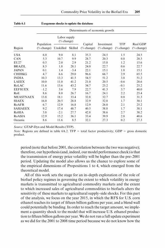
The GTAP database used here (v.6) is benchmarked to 2001; therefore, we undertake a historical update experiment to 2008 following the approach utilized by Beckman, Hertel, and Tyner (2011). Those authors show that by shocking population, labor supply, capital, investment and productiv-ity changes (see table 6.1), along with the relevant energy price shocks, the resulting equilibrium offers a reasonable approximation to key features of the more recent economy.
This updating of the model also allows us the opportunity to test the model’s ability to replicate the strengthened relationship between energy and agricultural prices. We do so by implementing the very same stochastic shocks used for the validation experiment in 2001, only now on our updated 2008 economy. As fi gure 6.1 illustrates, the observed correlation between oil and corn prices strengthened considerably over the 2001 to 2008 time
Commodity Price Volatility in the Biofuel Era 205
period (note that before 2001, the correlation between the two was negative); therefore, our hypothesis (and, indeed, our model performance check) is that the transmission of energy price volatility will be higher than the pre- 2001 period. Updating the model also allows us the chance to explore some of the empirical dimensions of Propositions 1 to 4, which emerged from the theoretical model.
All of this work sets the stage for an in- depth exploration of the role of biofuel policy regimes in governing the extent to which volatility in energy markets is transmitted to agricultural commodity markets and the extent to which increased sales of agricultural commodities to biofuels alters the sensitivity of these markets to agricultural supply- side shocks. For this part of the analysis, we focus on the year 2015, in which the RFS for U.S. corn ethanol reaches its target of fi fteen billion gallons per year, and a blend wall could potentially be binding. In order to reach the target amount, we imple-ment a quantity shock to the model that will increase U.S. ethanol produc-tion to fi fteen billion gallons per year. We do not run a full update experiment as we did for the 2001 to 2008 time period because we do not know how the
Table 6.1 Exogenous shocks to update the database
Determinants of economic growth
Labor supply (% change)
Region Population (% change)
Capital (% change)
Investment (% change)
TFP (% change)
Real GDP (% change) Unskilled Skilled
USA 6.0 9.0 8.1 35.3 24.5 1.5 24.5CAN 5.3 10.7 9.9 28.7 20.3 0.8 20.3EU27 0.5 2.0 2.9 21.2 15.8 1.2 15.6BRAZIL 8.5 1.8 28.1 24.0 22.7 0.6 22.7JAPAN 0.1 1.4 –3.4 22.1 15.1 1.8 15.1CHIHKG 4.7 6.6 29.0 96.6 66.7 2.9 65.5INDIA 10.3 13.3 41.5 54.5 51.2 3.8 51.2LAEEX 10.0 11.0 41.2 21.0 20.5 –0.6 20.6RoLAC 11.6 13.6 43.2 34.7 25.2 –0.1 25.2EEFSUEX –1.2 3.6 7.9 22.7 41.3 3.7 40.0RoE 8.6 8.0 26.7 16.7 24.1 2.2 25.4MEASTNAEX 13.8 18.1 33.4 32.8 32.7 0.8 31.3SSAEX 16.0 20.5 28.8 32.9 32.8 1.7 30.1RoAFR 6.7 12.9 16.8 12.9 26.0 2.1 25.2SASIAEEX 9.2 17.4 48.7 40.5 38.8 1.7 38.1RoHIA 3.8 –2.1 27.7 42.8 38.6 2.7 38.2RoASIA 12.9 15.2 36.1 33.4 39.9 2.8 40.6Oceania 8.6 11.6 8.5 32.1 27.3 0.2 27.3
Source: GTAP- Dyn and Model Results (TFP).Note: Regions are defi ned in table 6A.2. TFP � total factor productivity; GDP � gross domestic product.
206 Thomas W. Hertel and Jayson Beckman
key exogenous variables will evolve over this future period.10 We assume that the distributions of supply- side shocks in agriculture and energy markets, as well as the interannual volatility in regional GDPs, remain unchanged from their historical values; this has the virtue of allowing us to isolate the impact of the changing structure of the economy on corn price volatility.
Based on Proposition 4, we hypothesize that, at low oil prices, stochas-tic draws in the presence of a binding RFS will render corn markets more sensitive to agricultural supply- side shocks because a substantial portion of the corn market (the mandated ethanol use) will be insensitive to price, while at high corn prices, the opposite will be true, due to the highly elastic demand for ethanol as a substitute for corn. On the other hand, again, based on Proposition 4, we expect energy market volatility to have relatively little impact on corn markets at low oil prices.
At high oil prices, there are two possibilities—in the fi rst case, the RFS is nonbinding, and the blend wall is not a factor (i.e., it has recently been increased from 10 percent to 15 percent for recent model vehicles). In this case, we expect to see the infl uence of a larger share of corn going to ethanol () and also a larger share of ethanol going to the price- responsive portion of the fuel market (), translated into lesser sensitivity to random supply shocks emanating from the corn market (Proposition 1).
In the second case, high oil prices induce expansion of the ethanol indus-try to the point where the blend wall is binding so that Proposition 4 becomes relevant. In this case, the qualitative relationship between oil prices and corn prices is reversed; as with the binding RFS, the impact of random shocks to corn supply or demand will be magnifi ed with a binding blend wall.
Before investigating these hypotheses empirically, we must fi rst character-ize the extent of volatility in agricultural and energy markets. In terms of the PE model developed in the preceding, we must estimate the parameters underlying the distributions of �CS, �CD, and pF.
6.5 Characterizing Sources of Volatility in Energy and Agricultural Markets
The distributions of the stochastic shocks to corn production, corn demand, and oil prices are assumed to be normally and independently dis-tributed. Given the great many uses of corn in the global economy, we pre-fer to shock the underlying determinant of economywide demand, namely GDP, allowing these shocks to vary by model region. Of course GDP shocks also result in oil price changes, and, in a separate line of work, we have focused on the ability of this model to reproduce observed oil price volatility
10. Obviously, we could use projections of key variables, but they would be uncertain, and we do not believe this would signifi cantly alter our fi ndings, which hinge primarily on the quantity and cost shares featured in equation (19).
Commodity Price Volatility in the Biofuel Era 207
based on GDP shocks and oil supply shocks. However, in this chapter, we prefer to perturb oil prices directly so that we may separately identify the impact of energy price shocks and more general shocks to the economy.
To characterize the systematic component in corn production, time series models are fi tted to National Agricultural Statistical Service (NASS) data on annual corn production (corn easily commands the largest share of coarse grains, the corresponding GTAP sector; hence, the focus on corn) over the time period of 1981 to 2008.11 For crude oil prices, we use Energy Informa-tion Administration (EIA) data on U.S. average price and average import price (we take a simple average of the two series) over the same time periods. Here, we use the variation in regional GDP to capture changes in aggregate demand in each of the markets.
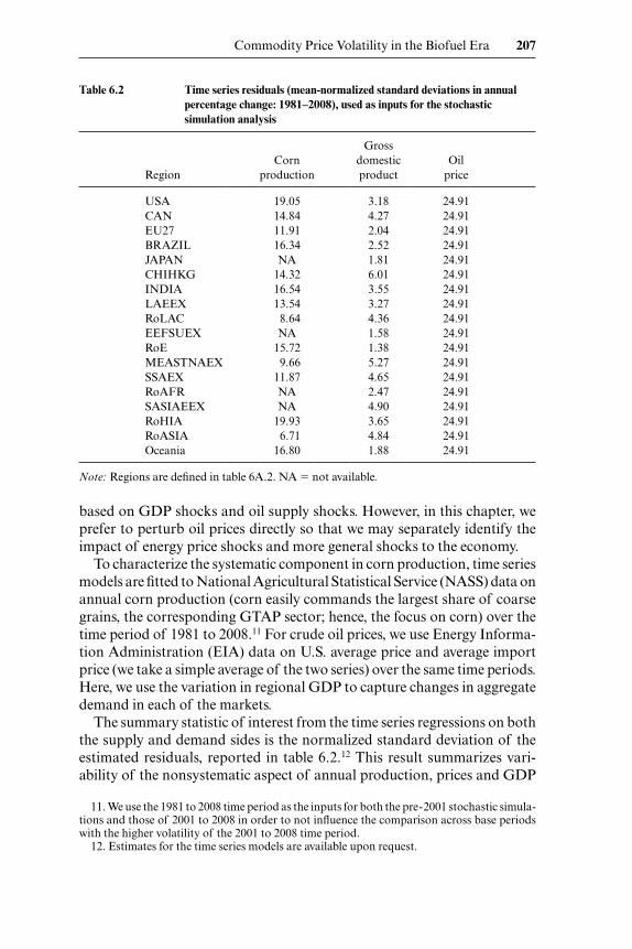
The summary statistic of interest from the time series regressions on both the supply and demand sides is the normalized standard deviation of the estimated residuals, reported in table 6.2.12 This result summarizes vari-ability of the nonsystematic aspect of annual production, prices and GDP
11. We use the 1981 to 2008 time period as the inputs for both the pre- 2001 stochastic simula-tions and those of 2001 to 2008 in order to not infl uence the comparison across base periods with the higher volatility of the 2001 to 2008 time period.
12. Estimates for the time series models are available upon request.
Table 6.2 Time series residuals (mean-normalized standard deviations in annual percentage change: 1981–2008), used as inputs for the stochastic simulation analysis
Region Corn
production
Gross domestic product
Oil price
USA 19.05 3.18 24.91CAN 14.84 4.27 24.91EU27 11.91 2.04 24.91BRAZIL 16.34 2.52 24.91JAPAN NA 1.81 24.91CHIHKG 14.32 6.01 24.91INDIA 16.54 3.55 24.91LAEEX 13.54 3.27 24.91RoLAC 8.64 4.36 24.91EEFSUEX NA 1.58 24.91RoE 15.72 1.38 24.91MEASTNAEX 9.66 5.27 24.91SSAEX 11.87 4.65 24.91RoAFR NA 2.47 24.91SASIAEEX NA 4.90 24.91RoHIA 19.93 3.65 24.91RoASIA 6.71 4.84 24.91
Oceania 16.80 1.88 24.91
Note: Regions are defi ned in table 6A.2. NA � not available.

208 Thomas W. Hertel and Jayson Beckman
in each region for the 1981 to 2008 time period (sectors and regions are defi ned in appendix tables 6A.1 and 6A.2). This is calculated as: √variance (of estimated residuals) divided by the mean value of production (or prices, or GDP), and multiplied by 100 percent. Not surprisingly, from table 6.2, we see that corn production and oil prices were much more volatile than GDP over the time period, with oil prices being somewhat more volatile than corn production. Note that we do not attempt to estimate region- specifi c variances for oil prices as we assume this to be a well- integrated global market.
6.6 Results for 2001 and 2008
6.6.1 Prebiofuel Era
Our fi rst task is to examine the performance of the model with respect to the 2001 base period. The fi rst pair of columns in table 6.3 reports the model- generated standard deviations in annual percentage change in coarse grains prices based on several alternative stochastic simulations undertaken using the Stroud Gaussian Quadrature as detailed in Arndt (1996) and Pear-son and Arndt (2000). In the fi rst column, we report the standard devia-tions in coarse grains prices when all three stochastic shocks from table 6.2 are simultaneously implemented. Focusing on the United States, the model with all three shocks predicts the standard deviation of annual percentage changes in corn prices to be 28.5, while the historical outcome (over the entire 1982 to 2008 period) revealed a standard deviation of just 20. So the model overpredicts volatility in corn markets. This is likely due to the fact that it treats producers and consumers as myopic agents who use only cur-rent information on planting and pricing to inform their production deci-sions. By incorporating forward- looking behavior as well as stockholding, we would expect the model to produce less price variation. Introducing more elastic consumer demand would be one way of mimicking such effects and inducing the model to more closely follow historical price volatility.
The second column under the 2001 heading reports the impact on coarse grains price volatility of oil price shocks only. From these results, it is clear that the energy price shocks have little impact on corn markets in the pre-biofuel era. In the United States, the amount of coarse grains price variation generated by oil price- only shocks is just a standard deviation of 1.1 percent, whereas the variation from the three sources is 28.5 percent (resulting in oil’s share of the total equaling 0.04, as reported in parentheses in table 6.3). This confi rms the fi ndings of Tyner (2009), who reports very little integration of crude oil and corn prices over the 1988 to 2005 period.
The third column in table 6.3 reports the observed variation in coarse grains prices from volatility in corn production. This indicates that the

Tab
le 6
.3
Mod
el- g
ener
ated
coa
rse
grai
n pr
ice
vari
atio
n in
200
1, 2
008,
and
201
5 ec
onom
ies
2001
mod
el v
olat
ility
2008
mod
el v
olat
ility
2015
mod
el v
olat
ility
(Bas
e- N
o R
FS/
BW
)
Reg
ion
A
ll sh
ocks
O
il pr
ice
C
orn
prod
ucti
on
All
shoc
ks
Oil
pric
e
Cor
n pr
oduc
tion
A
ll sh
ocks
O
il pr
ice
C
orn
prod
ucti
on
USA
28.5
1.1
(.04
)27
.5 (.
96)
30.7
10.0
(.32
)28
.7 (.
93)
29.8
15.6
(.53
)25
.1 (.
84)
CA
N16
.71.
1 (.
07)
16.2
(.97
)18
.84.
4 (.
23)
18.0
(.96
)18
.65.
5 (.
29)
17.7
(.95
)E
U27
18.3
1.0
(.05
)17
.5 (.
96)
20.4
3.1
(.15
)20
.0 (.
98)
20.2
3.2
(.16
)19
.8 (.
98)
BR
AZ
IL19
.01.
1 (.
06)
18.8
(.99
)21
.04.
3 (.
20)
20.7
(.99
)20
.64.
5 (.
22)
20.3
(.99
)JA
PAN
4.9
0.2
(.04
)3.
8 (.
77)
9.7
2.3
(.24
)8.
9 (.
92)
8.7
4.3
(.48
)7.
6 (.
88)
CH
IHK
G34
.00.
1 (0
)32
.4 (.
95)
47.0
1.8
(.04
)46
.4 (.
99)
46.3
0.8
(.02
)46
.0 (.
99)
IND
IA31
.41.
5 (.
05)
31.1
(.99
)37
.65.
1 (.
14)
36.9
(.98
)37
.53.
9 (.
10)
36.9
(.98
)L
AE
EX
18.7
1.0
(.05
)18
.1 (.
97)
20.4
5.0
(.25
)19
.8 (.
97)
20.2
5.8
(.29
)19
.5 (.
97)
RoL
AC
11.7
0.4
(.03
)11
.0 (.
95)
13.4
2.2
(.16
)12
.8 (.
96)
13.0
3.4
(.26
)12
.5 (.
96)
EE
FSU
EX
2.4
1.1
(.49
)0.
7 (.
29)
2.9
1.8
(.65
)1.
5 (.
54)
2.9
1.3
(.46
)1.
5 (.
52)
RoE
20.7
1.9
(.09
)20
.4 (.
99)
22.2
3.8
(.17
)22
.2 (1
.00)
22.0
3.7
(.17
)22
.0 (1
.00)
ME
AST
NA
EX
11.4
3.4
(.29
)10
.8 (.
94)
14.7
10.2
(.70
)12
.9 (.
88)
14.9
8.8
(.59
)12
.7 (.
85)
SSA
EX
2.8
2.6
(.92
)0.
7 (.
26)
6.1
9.5
(1.5
6)1.
0 (.
17)
6.1
7.6
(1.2
5)1.
0 (.
17)
RoA
FR
3.0
0.6
(.19
)1.
9 (.
64)
5.4
2.1
(.39
)4.
7 (.
88)
5.3
2.9
(.55
)4.
2 (.
79)
SASI
AE
EX
5.4
0.2
(.03
)4.
0 (.
74)
6.4
0.5
(.07
)5.
6 (.
87)
6.2
1.0
(.16
)5.
4 (.
88)
RoH
IA4.
80.
6 (.
12)
3.7
(.77
)6.
11.
0 (.
16)
5.6
(.91
)5.
61.
8 (.
31)
4.9
(.88
)R
oASI
A12
.30.
4 (.
04)
11.7
(.95
)13
.31.
1 (.
09)
12.9
(.96
)13
.10.
3 (.
02)
12.7
(.97
)O
cean
ia18
.90.
5 (.
03)
18.5
(.98
)19
.83.
0 (.
15)
19.1
(.96
)19
.24.
2 (.
22)
18.6
(.97
)W
orld
ave
rage
14
.4
16.3
15
.5
Not
es: N
umbe
rs in
par
enth
eses
rep
rese
nt th
e sh
are
of v
olat
ility
for
oil p
rice
/cor
n pr
oduc
tion
inpu
ts in
tota
l vol
atili
ty. H
isto
rica
l var
iati
on in
cor
n pr
ices
for
the
Uni
ted
Stat
es w
as 2
1.6
stan
dard
dev
iati
ons
over
the
1981
–200
8 ti
me
peri
od. R
egio
ns a
re d
efi n
ed in
tabl
e 6A
.2
210 Thomas W. Hertel and Jayson Beckman
majority of corn price variation in this historical period (a 0.96 share of the total) was due to volatility in corn production.
6.6.2 Biofuel Era
As discussed in the preceding section, we update the data base to 2008 in order to provide a reasonably current representation of the global economy in the context of the biofuel era. We then redo the same stochastic simula-tion experiments as 2001 to explore the energy or agricultural commodity price transmission in the biofuel era. The middle set of columns in table 6.3 present the results from this experiment.
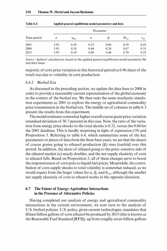
The model estimates somewhat higher overall coarse grain price variation (standard deviation of 30.7 percent) in this case. Now, the ratio of the varia-tion from energy price shocks to the total shocks is 0.32, versus the 0.04 for the 2001 database. This is hardly surprising in light of expression (19) and Proposition 3. Referring to table 6.4, which summarizes some of the key parameters or pieces of data from the three base years, we see that the shares of coarse grains going to ethanol production () rises fourfold over this period. In addition, the share of ethanol going to the price- sensitive side of the ethanol market () nearly doubles, and the net supply elasticity of corn to ethanol falls. Based on Proposition 3, all of these changes serve to boost the responsiveness of corn pries to liquid fuel prices. Meanwhile, the contri-bution of corn supply shocks to total volatility is somewhat reduced, as we would expect from the larger values for , , and �CE, although the smaller net supply elasticity of corn to ethanol works in the opposite direction.
6.7 The Future of Energy- Agriculture Interactions in the Presence of Alternative Policies
Having completed our analysis of energy and agricultural commodity interactions in the current environment, we now turn to the analysis of U.S. biofuel policies. U.S. policy, given current technologies, mandates that fi fteen billion gallons of corn ethanol be produced by 2015 (this is known as the Renewable Fuel Standard [RFS]), up from roughly seven billion gallons
Table 6.4 Applied general equilibrium model parameters and data
Parameter
Time period ! �FD $CE �EC
2001 3.95 0.10 0.25 0.06 0.39 0.432008 3.95 0.10 0.44 0.26 0.67 0.312015 3.95 0.10 0.60 0.40 0.70 0.25
Source: Authors’ calculations, based on the applied general equilibrium model parameter fi le and data bases.
Commodity Price Volatility in the Biofuel Era 211
produced in 2008.13 We implement this mandate by increasing U.S. etha-nol production through an exogenous quantity increase, following Hertel, Tyner, and Birur (2010).
Mathematically, the RFS effectively provides a lower bound on ethanol production and may be represented via the following complementary slack-ness conditions, where S is the per unit subsidy required to induce additional use of ethanol by the price sensitive agents in our model, and QR is the ratio of observed ethanol use to the quota as specifi ed under the RFS:
S � 0 ⊥ (QRRFS � 1) � 0 which implies that either:
S � 0, (QRRFS � 1) � 0 (RFS is binding) or:
S � 0, (QRRFS � 1) � 0 (RFS is nonbinding)
Because producers do not actually receive a subsidy for meeting the RFS, the additional cost of producing liquid fuels must be passed forward to consum-ers. We accomplish this by simultaneously taxing the combined liquid fuel product by the full amount of the subsidy.
The key point regarding the RFS is that it is asymmetric. Thus, when the RFS is just binding [S � 0, (QRRFS – 1) � 0], any rise in the price of gasoline will increase ethanol production past the mandated amount because ethanol is now better able to compete with gasoline on an energy basis. In this case, corn demand (and price) will be responsive to changes in the oil price. In contrast, a decrease in the price of gasoline does nothing to ethanol produc-tion (i.e., it stays at the fi fteen billion gallon mark) as this is the mandated amount; S � 0 ensures that the ethanol continues to be used at current levels. Of course, if the RFS is severely binding [S �� 0, (QRRFS – 1) � 0], then oil prices will have to rise considerably before reaching the point where S � 0 and the fuel price begins to translate through to the corn price. Because it is very difficult to predict whether the RFS will be binding in 2015, and if so, how severely binding it will be, we adopt the simple assumption that the RFS is just barely binding in the initial equilibrium. Therefore, any rise in oil prices will translate through to corn prices.
A blend wall works differently from the RFS; as pointed out by Tyner (2009), the blend wall is an effective constraint on demand.14 Mathemati-cally, the blend wall provides an upper bound on the ethanol intensity of liquid fuels and may be represented via the following complementary slack-
13. The RFS also mandates the production of advanced biofuels, which we do not consider here.
14. The Energy Information Agency estimates U.S. gasoline consumption at approximately 135 billion gallons; therefore, if the entire amount was blended with ethanol, we would fall short of the fi fteen billion gallon mark. Several alternatives have been suggested, such as improving E85 demand and increasing the blending regulation (this is currently being investigated by the Environmental Protection Agency) to 12 or 15 percent.
212 Thomas W. Hertel and Jayson Beckman
ness conditions, where T is the per unit tax required to restrict additional use of ethanol, and QR is the ratio of observed ethanol intensity (QE / QF) to the blend wall.
T � 0 ⊥ (1 � QRBW) � 0 which implies that either:
T � 0, (1 � QRBW) � 0 (BW is binding) or:
T � 0, (1 � QRBW) � 0 (BW is nonbinding)
For illustrative purposes, consider the case in which the blendwall is just barely binding so that T � 0, (1 – QRBW) � 0, but the RFS is not binding. Then if the price of gasoline were to rise, the ethanol intensity of liquid fuel use would not change because it is up against the blend wall. Of course, the overall level of ethanol production may well fall as total liquid fuel consump-tion falls, thereby dragging down the maximum amount of ethanol that can be added. In this case, the tax adjusts to ensure the constraint remains binding. However, if the price of gasoline falls, the ethanol intensity of pro-duction will decline, thereby moving off this constraint such that the blend wall becomes nonbinding.
As with the RFS, it is difficult to predict the extent to which the blend wall will be binding in 2015. However, given the strong political interest in maintaining ethanol production, at the time of the NBER conference (Spring 2010), we viewed it as likely that the blend wall would be adjusted upward in the future in order to permit the industry to meet the RFS. At the time of our revision of this chapter, this has indeed been done by the U.S. Environmental Protection Agency (EPA), with the blend rate for recent model vehicles now raised to 15 percent. It seems unlikely that E85 (a fuel blend comprising 85 percent ethanol) use will expand greatly in the United States due to infrastructure limitations (the fl ex- fuel auto stock is limited, and for this reason, the number of fuel stations offering E85 is also quite limited); therefore, it is reasonable to consider the case wherein the blend wall is adjusted such that it is just becoming binding at the 2015 RFS level.
Given the many different combinations of RFS and blend wall policy regimes, we investigate the importance of energy price shocks on agricultural commodity prices under four different scenarios:
1. Base case: The RFS is not binding under any combination of com-modity market shocks, and the blend wall is ignored. We expect that this base case will offer the largest scope for energy price shocks to infl uence agricultural commodity price volatility. Results from this case are reported in the last part of table 6.3.
2. RFS is just binding: That is, corn ethanol production is precisely fi fteen billion gallons in 2015. In this case, if oil prices rise due to a random shock to the petroleum market, ethanol production will also rise as this fuel is substituted for the higher priced petroleum. However, the effect of declin-

Commodity Price Volatility in the Biofuel Era 213
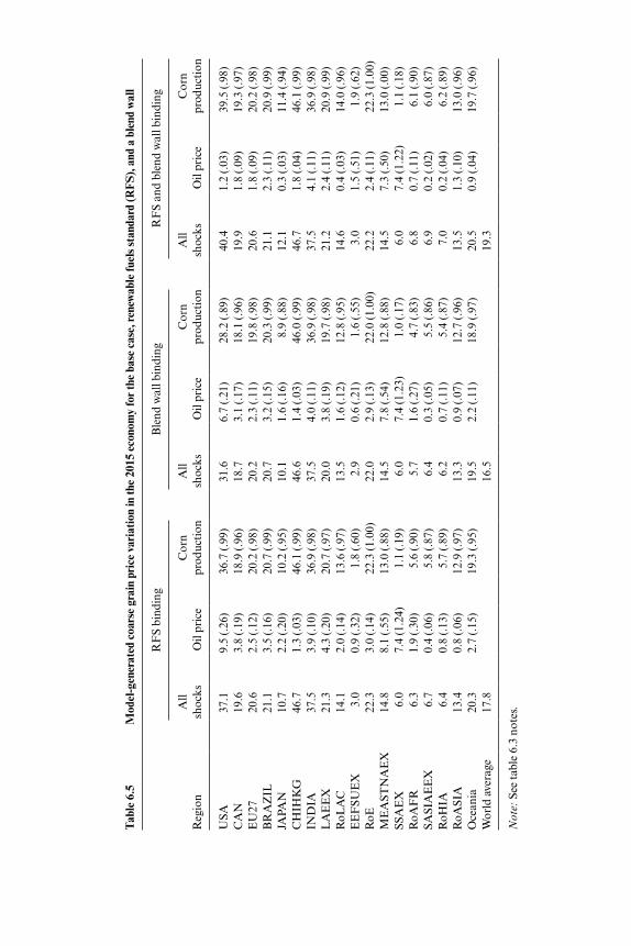
ing petroleum prices will not be translated back to the corn market as the RFS will prevent a contraction of ethanol production. This has the effect of making corn demand more inelastic such that commodity price volatility is greater in the wake of the supply- side shocks. Results from this and the subsequent experiments are reported in table 6.5.
3. RFS is not binding; however, the blend wall is binding: In this case, we assume that the strength of the overall economy as well as the relative prices of petroleum and corn in 2015 are such that ethanol production is well above the level specifi ed by the RFS so that the random shocks introduced in the following never threaten to push production below the fi fteen billion gallon annual target. However, in this case, the blend wall is very likely to be binding, and we specify the initial conditions in the model such that T � 0, (1 – QRBW) � 0; that is, the blend wall is on the verge of binding. In this case, we expect the impact of an oil price rise on corn price volatility to be very modest as it is not possible to increase the ethanol intensity of liquid fuels, so the only changes in ethanol use will be those emanating from changes in overall liquid fuel use.
4. RFS and blend wall are both on the verge of binding: This scenario could arise if the blend wall were continually adjusted upward, just reaching the point at which the RFS is met. In this case we have T � 0, (1 – QRBW) � 0 and S � 0, (QRRFS – 1) � 0.
Let us fi rst consider the 2015 base case results presented in table 6.3. These indicate that, relative to the 2008 database, in the absence of any role for the RFS and blend wall (BW), energy price shocks contribute more to coarse grain price variation. Indeed, energy price volatility now contributes to a standard deviation of 15.6, which amounts to 0.53 of the total variation in corn prices (but still less than the independent variation induced by corn supply- side shocks). This result is expected as even more corn is going to ethanol production (table 6.4), and there is double the amount of ethanol produced, compared to the 2008 database. In addition, ethanol production is free to respond to both low and high oil price draws from the stochastic simulations because the RFS and BW are nonbinding. The contribution of corn supply- side volatility shocks to corn price variation is also lowest for this case.
For the second scenario, we follow the same process as before to stimulate ethanol production to the RFS amount, and we run the same stochastic simulations; however, as noted previously, we assume that the RFS is initially just binding, and we implement the requirement that U.S. ethanol produc-tion cannot fall below fi fteen billion gallons. Results for this scenario indi-cate (refer to table 6.5) that the share of energy price volatility to total corn price variation is cut in half from the base case (from 0.53 to 0.26). This is due to the fact that we truncate consumers’ response to low oil price draws by using less ethanol. Implementation of the RFS also leads to much higher
Tab
le 6
.5
Mod
el- g
ener
ated
coa
rse
grai
n pr
ice
vari
atio
n in
the
2015
eco
nom
y fo
r th
e ba
se c
ase,
rene
wab
le fu
els
stan
dard
(RF
S),
and
a b
lend
wal
l
RF
S bi
ndin
gB
lend
wal
l bin
ding
RF
S an
d bl
end
wal
l bin
ding
Reg
ion
A
ll sh
ocks
O
il pr
ice
C
orn
prod
ucti
on
All
shoc
ks
Oil
pric
e
Cor
n pr
oduc
tion
A
ll sh
ocks
O
il pr
ice
C
orn
prod
ucti
on
USA
37.1
9.5
(.26
)36
.7 (.
99)
31.6
6.7
(.21
)28
.2 (.
89)
40.4
1.2
(.03
)39
.5 (.
98)
CA
N19
.63.
8 (.
19)
18.9
(.96
)18
.73.
1 (.
17)
18.1
(.96
)19
.91.
8 (.
09)
19.3
(.97
)E
U27
20.6
2.5
(.12
)20
.2 (.
98)
20.2
2.3
(.11
)19
.8 (.
98)
20.6
1.8
(.09
)20
.2 (.
98)
BR
AZ
IL21
.13.
5 (.
16)
20.7
(.99
)20
.73.
2 (.
15)
20.3
(.99
)21
.12.
3 (.
11)
20.9
(.99
)JA
PAN
10.7
2.2
(.20
)10
.2 (.
95)
10.1
1.6
(.16
)8.
9 (.
88)
12.1
0.3
(.03
)11
.4 (.
94)
CH
IHK
G46
.71.
3 (.
03)
46.1
(.99
)46
.61.
4 (.
03)
46.0
(.99
)46
.71.
8 (.
04)
46.1
(.99
)IN
DIA
37.5
3.9
(.10
)36
.9 (.
98)
37.5
4.0
(.11
)36
.9 (.
98)
37.5
4.1
(.11
)36
.9 (.
98)
LA
EE
X21
.34.
3 (.
20)
20.7
(.97
)20
.03.
8 (.
19)
19.7
(.98
)21
.22.
4 (.
11)
20.9
(.99
)R
oLA
C14
.12.
0 (.
14)
13.6
(.97
)13
.51.
6 (.
12)
12.8
(.95
)14
.60.
4 (.
03)
14.0
(.96
)E
EF
SUE
X3.
00.
9 (.
32)
1.8
(.60
)2.
90.
6 (.
21)
1.6
(.55
)3.
01.
5 (.
51)
1.9
(.62
)R
oE22
.33.
0 (.
14)
22.3
(1.0
0)22
.02.
9 (.
13)
22.0
(1.0
0)22
.22.
4 (.
11)
22.3
(1.0
0)M
EA
STN
AE
X14
.88.
1 (.
55)
13.0
(.88
)14
.57.
8 (.
54)
12.8
(.88
)14
.57.
3 (.
50)
13.0
(.00
)SS
AE
X6.
07.
4 (1
.24)
1.1
(.19
)6.
07.
4 (1
.23)
1.0
(.17
)6.
07.
4 (1
.22)
1.1
(.18
)R
oAF
R6.
31.
9 (.
30)
5.6
(.90
)5.
71.
6 (.
27)
4.7
(.83
)6.
80.
7 (.
11)
6.1
(.90
)SA
SIA
EE
X6.
70.
4 (.
06)
5.8
(.87
)6.
40.
3 (.
05)
5.5
(.86
)6.
90.
2 (.
02)
6.0
(.87
)R
oHIA
6.4
0.8
(.13
)5.
7 (.
89)
6.2
0.7
(.11
)5.
4 (.
87)
7.0
0.2
(.04
)6.
2 (.
89)
RoA
SIA
13.4
0.8
(.06
)12
.9 (.
97)
13.3
0.9
(.07
)12
.7 (.
96)
13.5
1.3
(.10
)13
.0 (.
96)
Oce
ania
20.3
2.7
(.15
)19
.3 (.
95)
19.5
2.2
(.11
)18
.9 (.
97)
20.5
0.9
(.04
)19
.7 (.
96)
Wor
ld a
vera
ge
17.8
16
.5
19.3
Not
e: S
ee ta
ble
6.3
note
s.
Commodity Price Volatility in the Biofuel Era 215
variation in corn prices. In Proposition 3, we demonstrated the cause of this; that is, the RFS severs the consumer demand- driven link between liquid fuels price and corn prices in the presence of low oil prices. The absence of price responsiveness in this important sector translates into a magnifi cation of the responsiveness of corn prices to random shocks to corn supplies and nonethanol demand.
These results are similar to those from Yano, Blandford, and Surry (2010), who use Monte Carlo simulations of a PE model to show that the U.S. etha-nol mandate reduces the impact that variations in petroleum prices have on corn prices (compared to a “no- mandate” scenario), while the impacts from variations in corn supply on corn prices are increased.
For the third scenario, we allow the RFS to be nonbinding, but we imple-ment a blend wall, which itself is assumed to be just binding. The results from this case indicate that the share of energy price volatility in total corn price variation is even lower than when the RFS is just binding. This is sub-stantiated by Tyner (2009), who notes that the blend wall effectively breaks the link between crude oil and corn prices as ethanol cannot react to high oil prices, but at low oil prices, the blend wall does little to reduce demand for ethanol.
The fi nal scenario in table 6.5 is the case wherein both the RFS and the BW are on the verge of binding. This largely eliminates the demand- side feedback from energy prices to the corn market, which is what we see in the results, with oil price volatility accounting for just 0.03 of the total variation in corn prices. In contrast, the price responsiveness of corn to supply- side shocks is greatly increased. Indeed, when compared to the 2015 base case (no RFS, no BW), corn price volatility in the face of identical supply side shocks is 57 percent greater. If we look at the fi nal row of table 6.5, we see that global price volatility is much increased under this scenario, rising by about one- quarter. Clearly the presence of biofuel mandates and associated fuel blending limits have the potential to greatly destabilize agricultural com-modity markets in the future.
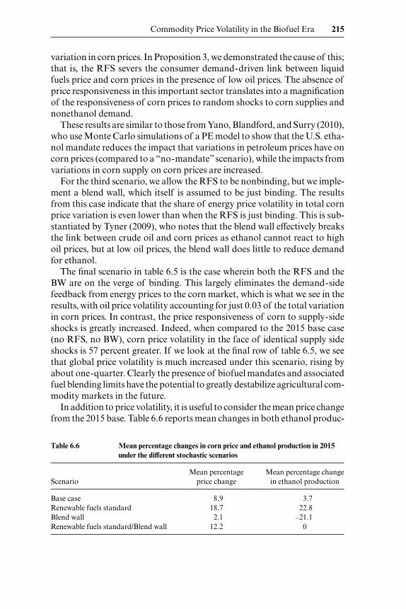
In addition to price volatility, it is useful to consider the mean price change from the 2015 base. Table 6.6 reports mean changes in both ethanol produc-
Table 6.6 Mean percentage changes in corn price and ethanol production in 2015 under the different stochastic scenarios
Scenario Mean percentage
price change Mean percentage change
in ethanol production
Base case 8.9 3.7Renewable fuels standard 18.7 22.8Blend wall 2.1 –21.1Renewable fuels standard/Blend wall 12.2 0

216 Thomas W. Hertel and Jayson Beckman
tion and corn prices in the United States under different policy regimes. Due to the nature of the demand relationships in the model, production short-falls generate larger price changes than do symmetric instances of excess production, and the mean corn price change under the base case is greater than zero. When the RFS and blend wall are both binding, ethanol pro-duction is unchanged, and the mean change in corn price is even larger, at 12.2 percent. When only the RFS is binding, instances of high corn prices—potentially due to a production shortfall—are rewarded with persistent ethanol demand due to the mandate. This has a tendency to boost mean ethanol production as well as mean corn prices. On the other hand, when only the blend wall is binding, episodes of low corn prices—possibly due to a favorable draw from the coarse grains productivity distribution—no longer result in greater ethanol production as the blend wall prevents further expansion. However, high corn prices do result in lower ethanol use, which is why the mean change in ethanol production is – 21 percent under the BW scenario. This results in lower expected corn prices as well.
6.8 Discussion
The relationship between agricultural and energy commodity markets has strengthened signifi cantly with the recent increase in biofuel produc-tion. Energy has always played an important role in agricultural production inputs; however, the combination of recent high energy prices with policies aimed at promoting energy security and renewable fuel use have stimulated the use of crop feedstocks in biofuel production. With a mandate to fur-ther increase biofuel production in the United States, it is clear that the relationship among agricultural and energy commodities may grow even stronger.
Results from this work indicate that the era of rapid biofuel production strengthened the transmission of energy price volatility into agricultural commodity price variation. The additional mandated production has the potential to further strengthen this transmission. However, the outcome will depend critically on the policy regime in which ethanol markets fi nd themselves. The presence of a Renewable Fuels Standard can hinder the ethanol’s sector’s ability to react to low oil prices, thereby destabilizing com-modity markets. The presence of a liquid fuels blend wall causes a similar disconnection in the transmission of energy prices to agriculture—albeit at high oil prices—and, therefore, also serves to increase commodity price volatility.
Comparing all the scenarios considered here, the absence of all biofuel policies leads to the highest transmission of energy price volatility into com-modity price variation and the lowest corn price volatility in response to tra-ditional supply- side shocks. This is because consumers are able to respond
Commodity Price Volatility in the Biofuel Era 217
to both high and low oil prices by changing their biofuel mix, and adjust-ment to corn supply shocks are absorbed by energy and nonenergy markets alike. When we implement biofuels policy (either the RFS or a blend wall), the impacts from energy price volatility are smaller than the base case, while the impacts from corn supply volatility are magnifi ed. In the most extreme case, wherein the blend wall is expanded to the point where the RFS is just barely binding, U.S. coarse grains price volatility in response to corn supply shocks is 57 percent higher than in the nonbinding case, and world price volatility is boosted by 25 percent. This underscores the point made by Irwin and Good (2010), who highlight the risk introduced by sizable sales of corn for ethanol production in the United States, particularly in light of mandated minimum purchases. They suggest that this could lead to record price rises in the wake of an extreme weather event in the Corn Belt of the United States—something that has not been observed during recent years. This leads them to advocate introducing some type of safety valve for the biofuels program.
In summary, it seems likely we will experience a future in which agricul-tural price volatility—particularly for biofuel feedstocks—may rise. The extent of this volatility will depend critically on renewable energy poli-cies. Indeed, in the future, these sources of uncertainty may become more important than traditional agricultural policies in many farm commodity markets.
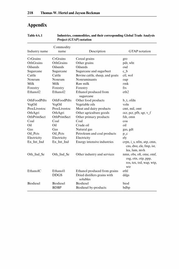
218 Thomas W. Hertel and Jayson Beckman
Appendix
Table 6A.1 Industries, commodities, and their corresponding Global Trade Analysis Project (GTAP) notation
Industry name Commodity
name Description GTAP notation
CrGrains CrGrains Cereal grains groOthGrains OthGrains Other grains pdr, whtOilseeds Oilseeds Oilseeds osdSugarcane Sugarcane Sugarcane and sugarbeet c_bCattle Cattle Bovine cattle, sheep, and goats ctl, wolNonrum Nonrum Nonruminants oapMilk Milk Raw milk rmkForestry Forestry Forestry frsEthanol2 Ethanol2 Ethanol produced from
sugarcaneeth2
OthFoodPdts OthFoodPdts Other food products b_t, ofdnVegOil VegOil Vegetable oils volnProcLivestoc ProcLivestoc Meat and dairy products cmt, mil, omtOthAgri OthAgri Other agriculture goods ocr, pcr, pfb, sgr, v_fOthPrimSect OthPrimSect Other primary products fsh, omnCoal Coal Coal coaOil Oil Crude oil oilGas Gas Natural gas gas, gdtOil_Pcts Oil_Pcts Petroleum and coal products p_cElectricity Electricity Electricity elyEn_Int_Ind En_Int_Ind Energy intensive industries crpn, i_s, nfm, atp, cmn,
cns, dwe, ele, fmp, isr, lea, lum, mvh
Oth_Ind_Se Oth_Ind_Se Other industry and services nmn, obs, ofi , ome, omf, osg, otn, otp, ppp,
ros, tex, trd, wap, wtp, wtr
EthanolC Ethanol1 Ethanol produced from grains ethlDDGS Dried distillers grains with
solublesddgs
Biodiesel Biodiesel Biodiesel biod BDBP Biodiesel by- products bdbp
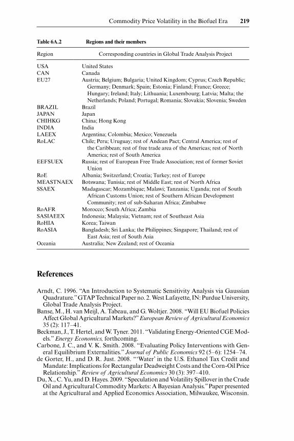
Commodity Price Volatility in the Biofuel Era 219
References
Arndt, C. 1996. “An Introduction to Systematic Sensitivity Analysis via Gaussian Quadrature.” GTAP Technical Paper no. 2. West Lafayette, IN: Purdue University, Global Trade Analysis Project.
Banse, M., H. van Meijl, A. Tabeau, and G. Woltjer. 2008. “Will EU Biofuel Policies Affect Global Agricultural Markets?” European Review of Agricultural Economics 35 (2): 117– 41.
Beckman, J., T. Hertel, and W. Tyner. 2011. “Validating Energy- Oriented CGE Mod-els.” Energy Economics, forthcoming.
Carbone, J. C., and V. K. Smith. 2008. “Evaluating Policy Interventions with Gen-eral Equilibrium Externalities.” Journal of Public Economics 92 (5– 6): 1254– 74.
de Gorter, H., and D. R. Just. 2008. “‘Water’ in the U.S. Ethanol Tax Credit and Mandate: Implications for Rectangular Deadweight Costs and the Corn- Oil Price Relationship.” Review of Agricultural Economics 30 (3): 397– 410.
Du, X., C. Yu, and D. Hayes. 2009. “Speculation and Volatility Spillover in the Crude Oil and Agricultural Commodity Markets: A Bayesian Analysis.” Paper presented at the Agricultural and Applied Economics Association, Milwaukee, Wisconsin.
Table 6A.2 Regions and their members
Region Corresponding countries in Global Trade Analysis Project
USA United StatesCAN CanadaEU27 Austria; Belgium; Bulgaria; United Kingdom; Cyprus; Czech Republic;
Germany; Denmark; Spain; Estonia; Finland; France; Greece; Hungary; Ireland; Italy; Lithuania; Luxembourg; Latvia; Malta; the Netherlands; Poland; Portugal; Romania; Slovakia; Slovenia; Sweden
BRAZIL BrazilJAPAN JapanCHIHKG China; Hong KongINDIA IndiaLAEEX Argentina; Colombia; Mexico; VenezuelaRoLAC Chile; Peru; Uruguay; rest of Andean Pact; Central America; rest of
the Caribbean; rest of free trade area of the Americas; rest of North America; rest of South America
EEFSUEX Russia; rest of European Free Trade Association; rest of former Soviet Union
RoE Albania; Switzerland; Croatia; Turkey; rest of EuropeMEASTNAEX Botswana; Tunisia; rest of Middle East; rest of North AfricaSSAEX Madagascar; Mozambique; Malawi; Tanzania; Uganda; rest of South
African Customs Union; rest of Southern African Development Community; rest of sub- Saharan Africa; Zimbabwe
RoAFR Morocco; South Africa; ZambiaSASIAEEX Indonesia; Malaysia; Vietnam; rest of Southeast AsiaRoHIA Korea; TaiwanRoASIA Bangladesh; Sri Lanka; the Philippines; Singapore; Thailand; rest of
East Asia; rest of South AsiaOceania Australia; New Zealand; rest of Oceania
220 Thomas W. Hertel and Jayson Beckman
Gellings, C., and K. E. Parmenter. 2004. “Energy Efficiency in Fertilizer Production and Use.” In Efficient Use and Conservation of Energy, edited by C. W. Gellings and K. Blok, in Encyclopedia of Life Support Systems (EOLSS). Oxford, UK: Eolls. http:/ / www.eolss.net.
Gohin, A., and F. Chantret. 2010. “The Long- Run Impact of Energy Prices on World Agricultural Markets: The Role of Macro- Economic Linkages.” Energy Policy 38 (1): 333– 39.
Gohin, A., and D. Tréguer. 2010. “On the (De) Stabilization Effects of Biofuels: Relative Contributions of Policy Instruments and Market Forces.” Journal of Agricultural and Resource Economics 35 (1): 72– 86.
Grassini, M. 2004. “Rowing along the Computable General Equilibrium Modeling Mainstream.” Paper presented at conference, Input- Output and General Equilib-rium Data, Modeling, and Policy Analysis, Brussels, Belgium.
Hertel, T. W. 1999. “Future Directions in Global Trade Analysis.” GTAP Working Paper no. 4. West Lafayette, IN: Center for Global Trade Analysis. http:/ / www.gtap.agecon.purdue.edu/ resources/ working_papers.asp.
Hertel, T. W., A. Golub, A. Jones, M. O’Hare, R. Plevin, and D. Kammen. 2010. “Global Land Use and Greenhouse Gas Emissions Impacts of U.S. Maize Etha-nol: Estimating Market- Mediated Responses.” BioScience 60 (3): 223– 31. forth-coming.
Hertel, T. W., W. E. Tyner, and D. K. Birur. 2010. “Global Impacts of Biofuels.” Energy Journal 31 (1): 75– 100.
Hochman, G., S. Sexton, and D. Zilberman. 2008. “The Economics of Biofuel Pol-icy and Biotechnology.” Journal of Agricultural and Food Industrial Organization 6 (2), doi:10.2202/ 1542- 0485.1237.
Irwin, S., and D. Good. 2010. “Alternative 2010 Corn Production Scenarios and Policy Implications.” Marketing and Outlook Brief. University of Illinois, Depart-ment of Agricultural and Consumer Economics, March 11.
Jorgenson, D. 1984. “Econometric Methods for Applied General Equilibrium Anal-ysis.” In Applied General Equilibrium Analysis, edited by H. E. Scarf and J. B. Shoven, 139– 203. New York: Cambridge University Press.
Keeney, R., and T. Hertel. 2009. “The Indirect Land Use Impacts of United States Biofuel Policies: The Importance of Acreage, Yield, and Bilateral Trade Response.” American Journal of Agricultural Economics 91 (4): 895– 909.
Kehoe, T. 2003. “An Evaluation of the Performance of Applied General Equilibrium Models of the Impact of NAFTA.” Federal Reserve Bank of Minneapolis, Research Department Staff Report no. 320.
McPhail, L., and B. Babcock. 2008. “Ethanol, Mandates, and Drought: Insights from a Stochastic Equilibrium Model of the U.S. Corn Market.” Working Paper no. 08- WP 464. Iowa State University, Center for Agricultural and Rural Develop-ment.
Meyer, S., and W. Thompson. 2010. “Demand Behavior and Commodity Price Volatility under Evolving Biofuel Markets and Policies.” In Handbook of Bioen-ergy Economics and Policy, edited by M. Khanna, J. Scheffran, and D. Zilberman, 133– 50. New York: Springer Science Verlag.
Pearson K., and C. Arndt. 2000. “Implementing Systematic Sensitivity Analysis Using GEMPACK.” GTAP Technical Paper no. 3. West Lafayette, IN: Purdue University, Global Trade Analysis Project.
Searchinger, T., R. Heimlich, R. A. Houghton, F. Dong, A. Elobeid, J. Fabiosa, S. Tokgoz, D. Hayes, and T.- H. Yu. 2008. “Use of U.S. Croplands for Biofuels Increases Greenhouse Gases through Emissions from Land Use Change.” Science 319:1238– 40.

Commodity Price Volatility in the Biofuel Era 221
Serra, T., D. Zilberman, J. M. Gil, and B. K. Goodwin. 2010a. “Price Transmission in the U.S. Ethanol Market.” In Handbook of Bioenergy Economics and Policy, edited by M. Khanna, J. Scheffran, and D. Zilberman, 55– 72. New York: Springer Science Verlag.
———. 2010b. “Price Volatility in Ethanol Markets.” Unpublished Manuscript. Energy Bioscience Institute, University of California, Berkeley.
Taheripour, F., D. Birur, T. Hertel, and W. Tyner. 2007. “Introducing Liquid Bio -fuels into the GTAP Data Base.” GTAP Research Memorandum no. 11. West La fayette, IN: Purdue University, Global Trade Analysis Project.
Taheripour, F., T. Hertel, W. Tyner, J. Beckman, and D. Birur. 2009. “Biofuels and Their By- products: Global Economic and Environmental Implications.” Biomass and Bioenergy 33 (3): 278– 89.
Thompson, W., S. Meyer, and P. Westhoff. 2009. “How Does Petroleum Price and Corn Yield Volatility Affect Ethanol Markets with and without an Ethanol Use Mandate?” Energy Policy 37 (2): 745– 49.
Tyner, W. 2009. “The Integration of Energy and Agricultural Markets.” Paper pre-sented at the International Association of Agricultural Economists, Beijing, China.
Ubilava, D., and M. Holt. 2010. “Forecasting Corn Prices in the Ethanol Era.” Unpublished Manuscript. Department of Agricultural Economics, Purdue Uni-versity.
Valenzuela, E., T. W. Hertel, R. Keeney, and J. Reimer. 2007. “Assessing Global Computable General Equilibrium Model Validity Using Agricultural Price Vola-tility.” American Journal of Agricultural Economics 89 (2): 383– 97.
Yano, Y., D. Blandford, and Y. Surry. 2010. “The Impact of Feedstock Supply and Petroleum Price Variability on Domestic Biofuel and Feedstock Markets—The Case if the United States.” Swedish University of Agricultural Sciences Working Paper no. 2010:3. Uppsala, Sweden: Swedish University of Agricultural Sciences.