1

The Intergenerational Dynamics of Social Inequality –

Empirical Evidence from Europe and the United States

Veronika V. EBERHARTER University of Innsbruck, Department of Economics,

Universitaetsstrasse 15/3, A-6020 INNSBRUCK, Austria, e-mail: veronika.eberharter@uibk.ac.at

Abstract

Based on nationally representative data from the German Socio-Economic Panel

(GSOEP), the Panel Study of Income Dynamics (PSID), and the British Household

Panel Survey (BHPS) we analyze the intergenerational transmission of economic and

social (dis-)advantages in Germany, the United States and Great Britain. We test with

the hypotheses that extent and determinants of intergenerational income mobility

and the relative risk of poverty differ with respect to the existing welfare state

regime, family role patterns, and social policy design. The empirical results indicate

a higher intergenerational income elasticity in the United States than in Germany and

Great Britain, and country differences concerning the influence of individual and

parental socio-economic characteristics, family disruption and health dissatisfaction

on intergenerational income mobility and the relative risk of poverty.

Key words: Social and economic inequality; Intergenerational income mobility; poverty, social exclusion; JEL-Classifications: D31 Personal Income, wealth, and their distribution; J24 Human capital; J62 Job, Occupational, and Intergenerational Mobility;

2

1. Introduction

Most of the industrialized countries are confronted by changing social and economic

structure, increasing economic and social inequalities, low income and social

isolation. The negative relation between income inequality and intergenerational

income mobility suggests that children growing up in low-income households can

only escape the poverty trap if intergenerational income mobility compensates

economic and social inequality (Mayer and Lopoo 2005). From the socio-political

point of view, the research of the determinants of intergenerational income mobility

and poverty persistence is essential to design effective social policy measures.

Though focused on alleviating social and economic inequalities, the social policy of a

country reproduces “stratification” in terms of power, class and other forms of

inequality. The policy instruments and transfer packages tell a great deal about the

working of a country’s welfare state regime. The welfare state regime defines a

complex of legal and organizational properties, and defines the role of the state,

interacting alongside the market, the civil society, and the family in the provision of

welfare (Therborn 1995, de Swaan 1988, Arts and Gelissen 2002). The existing

topologies of welfare state regimes are based on various dimensions, as social

insurance and poverty policy (Leibfried 1992, Korpi and Palme 1998), welfare

expenditures, benefit equality, and taxes (Castles and Mitchell 1993, Bonoli 1997,

Kauto 2002), female work desirability (Siaroff 1994), political tradition (Navarro and

Shi 2001), or decommodification and stratification (Esping-Andersen 1990, Esping-

Andersen 1994, Esping-Andersen 1999).

The Esping-Anderson welfare state regime typology clusters democratic industrial

societies into liberal, conservative, and social democratic welfare state regimes. The

liberal welfare state regime (United States, Great Britain, Canada, Australia, New

Zealand) is characterized by low decommodification and strong individualistic self-

relianceThe public philosophy is grounded on the idea of opportunity reflecting

individual efforts, which indicates an open, liberal and dynamic social system. The

distributional consequences of the market forces are accepted. A relatively

unregulated labor market fosters the creation of low-skill, and low-paid jobs, large

wage dispersions, and small differences in the jobs performed by women and men.

Labor market policies offer less protection for workers and do little to ameliorate

3

market-based risks. The market rather than the state is promoted in guaranteeing

the welfare needs of the citizens. These countries are characterized in terms of

minimal assistance to allow the worker the opportunity to gain entry back into the

market should circumstances dictate a temporary departure. The state reacts only in

case of social failures and limits the help to special groups. The transfers are modest

and the rules for entitlement are very strict. The principle of stratification leads to

low-income state dependents, and people able to afford social insurance plans and

the privately financed higher education. The education systems are less stratified and

standardized which may induce a higher social mobility. At the other hand higher

education is privately financed, which suggests intergenerational social immobility

(Couch and Dunn 1997, Mortimer and Krüger 2000, Charles et al. 2001, Hall and

Soskice 2001, Dustmann 2004, Gornick and Meyers 2003).

The conservative-corporatist welfare state regime (Germany, Austria, France, Italy) is

typified by a modest level of decommodification. Government policies ensure against

market-based risks and protect those who are unable to succeed in the market place.

The direct influence of the state is restricted to the provision of income maintenance

benefits. The labor market institutions and labor market policies ensure employment

stability. Health care, welfare, social insurance, national assistance, and old age

pensions are provided at government expense. Social policy is designed to

guarantee income equality. Family policies facilitate the incorporation of women into

the labor force (e.g. child care, paid maternity leave, job return guarantees) and

support the transition from the traditional male bread-winner model to the adult

worker model. At the other hand tax policy (e.g. tax splitting) favor men as

breadwinner and women foremost as mothers, which reinforce the preservation of

traditional family role patterns concerning the allocation of time into paid work

(Charles et al. 2001, Lewis 2006). The education system is formal and coordinated,

and higher education is publicly provided. In Germany, the vocation-oriented

educational “dual system” relies on occupation-specific credentials, and results in

socially stratified and sex segregated outcomes. The federal states have the primary

responsibility for organizing the educational system, which results in a high level of

standardization, and constitutes the mechanisms for perpetuating social inequalities

(Mortimer and Krüger 2000, OECD 2012).

4

The social democratic approach to welfare and social policy (Scandinavian countries)

is especially committed to create equal opportunity, to reduce social risks, and to

diminish social divisions. The level of decommodification is high, and stratification is

directed to achieve a system of highly distributive benefits. These countries advocate

full employment and promote equality including the provision of a safety net that no

one should be allowed to fall through. Social policy aims at maximizing the

capacities of individual independence. Women are encouraged to participate in the

labor market.

The paper aims to analyze the influence of the individual and parental socio-

economic mapping, and social exclusion characteristics on the intergenerational

income mobility and the relative risk of poverty in countries with different welfare

state regimes, labor market institutions, family role patterns, and social policy design.

The paper focuses on the situation in Germany, the United States, and Great Britain.

We test the hypotheses that the link between social stratification, intergenerational

income mobility, and poverty persistence works differently according to the existing

welfare state regime, family role patterns, and the social policy:

- In the United States and Great Britain we expect a higher income inequality which

is associated with a lower intergenerational income mobility than in Germany.

Due to the high self-relience and mobile society we expect that the impact of

family background characteristics on intergenerational income mobility and the

relative poverty risk is more expressed than in Germany.

- Due to the social policy design, focusing on a higher social permeability of the

society, we expect a higher intergenerational income mobility at the bottom of

the income distribution in Germany than in the United States and Great Britain.

- In all the countries, we suppose that instable family structures, non-employment,

and disability boost the relative risk of poverty.

To analyze the determinants of the intergenerational income mobility we employ a

regression approach on the permanent post-government income variables of children

and parents including a set of individual and family background controls (Solon 1999,

Björklund and Jäntti 2000, Hertz 2004, Couch and Lillard 2004, Grawe 2004). We

apply quintile transition matrices and the Bartholomew mobility index (Bartholomew

1982, Dearden et al. 1997) to evaluate the intergenerational mobility for different

5

income positions. To analyze the determinants of the relative poverty risk we employ

a binomial logit model (Mc Fadden 1973, Maddala 1983, Heckman 1981). The

explanatory variables contain a set of individual and family background socio-

economic resources, and social exclusion attributes.

The paper is organized in 5 sections: section 2 focuses on the theoretical background

of the intergenerational transmission of social and economic disadvantages, section 3

reports the data and sample organization, section 4 outlines the methodology to

analyse the intergenerational income mobility and the relative risk of poverty

conditional to individual and family background characteristics, and social exclusion

attributes. Section 5 presents the empirical results and section 6 concludes with a

summary of findings and discussion of some stylized facts about the

intergenerational heritage of economic and social disadvantages to derive policy

implications and directions for further research.

2. Theoretical Background

Poverty and social exclusion are dynamic processes limiting a person’s future

prospects (Atkinson 1998). Social exclusion is a multi-dimensional phenomenon,

affecting both the quality of life of individuals and the equity and cohesion of society

as a whole (Levitas et al. 2007). Social exclusion reflects a combination of inter-

related factors resulting from a lack of capabilities (Sen 1985, Sen 1992) required to

participate in economic and social life (poor skills, labor market exclusion, living in a

jobless household), service exclusion (public transport, gas, electricity, water,

telephone), exclusion from social relations (common activities, social networks),

exclusion from support available in normal times and in times of crisis, exclusion

from engagement in political and civic activity, poor housing, high crime

environment, disability, health problems, or family breakdown (Social Exclusion Unit

1997, Saunders et al. 2007, Saunders 2008). Poverty is either discussed as a

dimension of social exclusion (Marlier and Atkinson 2010) or a concept very close to

social exclusion. If poverty is understood as encompassing low income situations

implying a lack of participation in the key activities in social, political, and cultural life

(Townsend 1979, United Nations 1995, Duffy 1995, Walker and Walker 1997,

6

Burchard et al. 2002) or the inability to do things, that are in some sense

considered normal by society as a whole (Howarth et al. 1998), or the insufficiency

of different attributes of well-being (e.g. housing, literacy, health, provision of public

good, income, etc.), then both the concepts become very close (Bourguignon and

Chakravarty 2003).

There are two major theories concerning the mechanisms of the intergenerational

transmission of advantages and disadvantages. According to the family resource

model it is not a lack of economic resources, but other characteristics of the parents

that are correlated with the economic status that influence the parental abilities to

provide stimulating environments for their children to have economic success. Low-

income parents more likely possess disadvantageous characteristics, and therefore

they fail to provide stimulating environments for the better-off of their children

(Mayer 1997).

According to the neoclassical human capital approach (Becker 1964, Mincer 1974)

the economic status of the parents is transmitted to their children. The structural

hypothesis of intergenerational economic and social mobility emphasizes the view

that limited parental resources during childhood restrict the social and economic

status of the children as adults (Blanden et al. 2005, Mayer and Lopoo 2005). The

parental investments increase the children´s human capital, which in turn positively

affects their earnings capacity (Becker and Tomes 1986, Solon 1992, Solon 1999,

Solon 2002, Chadwick and Solon 2002, Mazumdar 2005) or their ability to gain non-

labor income, and even their success in the marriage market (Pencavel 1998).

Among the endowment conditions parental education, employment behaviour,

occupational choice, the family role patterns, as well as the social capital

environment are of importance (Stevens 1999, Finnie and Sweetman 2003). The

increasing social and economic inequalities in most of the industrialized countries

suggest increasing gaps in the parents’ investment abilities which impede the

economic success of the offspring (Acemoglu and Pischke 2000).

The first generation of the studies on intergenerational income mobility (Becker and

Tomes 1986) found an intergenerational correlation of income or earnings of about

.2 for the United States, implying that the parental status does not strongly affect the

children’s. The second generation of studies (Solon 1992, Solon 1999, Solon 2002)

7

found a higher intergenerational elasticity, using multi-year income measures and

correcting for measurement errors. The analysis of the dynamics of the

intergenerational income mobility (Corcoran 2001, Mayer and Lopoo 2002) reveals a

decreasing effect of the parental income status on the income and social position of

the children.

3. Data Base and Sample Organization

The empirical analysis is based on data from the German Socio-Economic Panel (SOEP), the

British Household Panel Survey (BHPS), and the US Panel Study of Income Dynamics (PSID),

which were made available to us by the Cross-National Equivalent File (CNEF) project at the

College of Human Ecology at Cornell University, Ithaca, N.Y..1 The PSID started in 1980

and contains a nationally representative unbalanced panel of about 40,000

individuals in the United States. From 1997 on the PSID data are available bi-yearly.

The GSOEP started in 1984 and contains a representative sample of about 29,000

German individuals that includes households in the former East Germany since 1990.

The BHSP started in 1991. The first wave consists of some 5,500 households and

10,300 individuals drawn from 250 areas of Great Britain. Additional samples of

1,500 households in each of Scotland and Wales were added in 1999, and in 2001 a

sample of 2,000 households was added in Northern Ireland, making the panel

suitable for UK-wide research. The surveys track the socioeconomic variables of a

given household, and each household member is asked detailed questions about age,

gender, marital status, educational level, labor market participation, working hours,

employment status, occupational position, economic situation of the members of a

given family over time, as well as household size and composition. The income

variables are measured on an annual basis and refer to the prior calendar year. The

data allow monitoring the employment and occupational status, the earnings

situation, and the socio-economic characteristics of the individuals.

The data do not provide a sufficiently long time horizon to observe parents and

children at identical life cycle situations, but cover an adequately long period to allow

monitoring socioeconomic characteristics, employment and occupational status, and

earnings situation of children living in the parental household and when becoming

1 For a detailed description of the data bases see Frick et al. (2007).

8

members of other family units. In this way the data allow to draw inferences about

the effects of being exposed to different life situations in the parental household on

the economic and social situation as young adults. The sample is restricted to

persons aged 14 to 20 years, and co-resident with their parents in four consecutive

years (United States (1987-1991), Germany (1988-1992), and Great Britain (1991-

1995). The data base does not allow identifying parents - children relations exactly,

therefore we define ‘parents’ as adults, whose marital status is ‘married’, or ‘living

with partner’ and who are living in households with persons indicated as ‘children’.

We use family (household) identifiers and relationship codes to match sons and

daughters to their fathers and mothers within each data set. We allow families to

contribute as many parent-child pairs to each data set as meet our screening rules:

the number of the parent-child pairs equals the number of the children in the

parental households. The young adults are at least 24 years old when we observe

the economic and social status in 2005-2009 (Germany) or 2003-2007 (USA), and in

2004-2008 (GB) when living in their own households. We focus on persons

participating in the labor market, and exclude persons in full-time education. We do

not consider the former East Germans, for they are not included in the GSOEP

sampling frame before 1990. We analyze the intergenerational economic and social

mobility of persons in Great Britain because other regions are not included in the first

waves of the British Household Panel Survey. The selection process leads to a

sample of 2,128 German women and men, the US sample covers 2,585 persons, and

the British sample includes 1,840 women and men.

We follow the standard conventions and assume that income is shared within

families and thus household income is arguably a better measure of the economic

and social status than individual income variables (Mazumdar 2005). The study is

based on the equivalent post-government household income, which equals the pre-

government household income plus household public transfers (social benefits:

dwellings, child or family allowances, unemployment compensation, assistance, and

other welfare benefits), plus household social security pensions (age, disability,

widowhood), deducting household total family taxes (mandatory social security

contributions, income taxes, or mandatory employee contributions). We use the

referred income variables from the data base, thus the results make not allowance

for the bias of imputed values on income inequality and income mobility (Frick and

9

Grabka 2005). To consider the family structure we calculate the permanent

household income per adult equivalent. Instead of the ‘modified’ OECD-equivalence

scale (Hagenaars et al. 1994) we employ the ‘old’ OECD-equivalence scale (OECD

1982) made available by the data base, which assigns a value of one to the first

adult household member, a value of 0.7 to each additional adult, and a value of 0.5

to each child. The household income variables are deflated with the national CPI

(2001=100) to reflect constant prices. To exclude transitory income shocks and

cross-section measurement errors we use 5-year moving averages of the real

equivalent post-government household income variables. The parental household

socio-economic mapping is captured either by the characteristics of the father or the

mother. In “double”-parent families the characteristics of the father are employed, in

“single”-parents families the characteristics of the mother or the father are

introduced in the analysis.

A major factor that will lead to changes in the quality of mobility data is that

response rates tend to decline over time and so the representativeness of mobility

tables derived from survey data may worsen. As the income variables highly

determine survey-attrition we follow Fitzgerald et. al. (1998a; 1998b) to construct a

set of sample specific weights to address to the non-random sample attrition bias,

that do not account for attrition in general, but for attrition among the particular

groups under study We estimate a probit equation that predicts retention in the

sample (i.e being observed as an adult) as a function of pre-determined variables

measured during childhood. Presuming that the samples are representative when the

children are still children we construct a set of weights

1Pr( 0 , )

( , )Pr( 0 )

A z xw z x

A x

− == =

M

M (1)

where x denotes the parental income as primary regressor, and z is a vector of

covariates to predict attrition, indicated by A=1. Thus w(z,x) will take higher values

for people whose characteristics z make them more likely to exit the panel before

their adult income can be measured. The variables considered in z are the gender,

and the parental age and educational attainment as well as their squares. We

suppose these variables to affect the attrition propensities, to be endogenous to the

10

outcome, that is to have an effect on the children’s income as adults conditional on

the parental income. The weights w(x,z) are multiplied with the parental household

weights, which yields a set of weights that apply to the household of the children as

adults. The parental household weights are assumed to capture the attrition effects

and the weights, w(z,x), compensate for subsequent non-random attrition.

4. Methodology

4.1 Intergenerational Income Mobility

The most common approach to quantify how economic (dis)advantages are

transmitted across generations is to estimate the intergenerational income elasticity

applying ordinary least squares (OLS) to the regression of a logarithmic measure of

the children’s income variable ( cy ) on a logarithmic measure of the income variable

of the parental household ( py ), and a set of control variables )( cX

0 12

n

c p c c cc

y ß ß y ß X ε=

= + + +∑ . (2)

In model specification (a) we regress the logarithm of the average equivalent post-

government income (2001=100) of the children’s generation on the logarithm of the

average equivalent post-government income (2001=100) of the parental household.

The constant term ß0 represents the change in the economic status common to the

children’s generation. The slope coefficient, 1β , is used as a measure of

intergenerational mobility and expresses the elasticity of the children’s income

variable with respect to the parents’ income situation. The larger 1β the more likely a

person will inhabit the same income position as her parents, which implies a greater

persistence of the intergenerational economic status. A 1β close to zero bears

evidence of an open society in which the economic situation of the parents has no

impact on the economic success of the children. The random error component cε is

usually assumed to be distributed ),0( 2σN .

The model specification (b) introduces a set of individual and family background

characteristics )( cX to account for the indirect effects of the parental income on the

11

children’s income. To the extent that these variables lower the coefficient ß1 these

other effects “account for” the raw intergenerational income elasticity. The gender

dummy (GEN) takes the value 1 for men and the value 0 for women and controls for

gender differences on intergenerational income elasticity. We include the years of

education of the individual (EDUC) to capture the human capital level. In the case of

missing values the educational attainment is set equal to the amount reported in the

previous year. The educational attainment of the parents (EDUCP) is included with

the average schooling years of the parents to capture the human capital hypothesis

that the higher the income of the parents the higher their investment in the

education of the children, which in turn causes a higher income of the children. The

number of children (CHILD) in the household considers the effects of care

requirements on the disposable household income. The effect of unemployment

phases in the parental household (UNEMPP) takes the value 1 if one of the parents is

employed less than half the observation period, and 0 else. We include four

occupational dummies to capture the social status of one of the individual’s parents

(OCCp). To avoid multicollinearity with the individual and parental income variables

we do not employ the ISEI (International Socio-Economic Index of Occupational

Status) classification of occupations, based on income, education and occupations

(Ganzeboom et al. 1992, Ganzeboom and Treimann 1996, Ganzeboom and Treimann

2003). The empirical specification of the occupational status is oriented at the ISCO-

88 (International Standard Classification of Occupations). ISCO-88 aggregates the

occupations into broadly similar categories in an hierarchical framework according to

the degree of complexity of constituent tasks and skill specialization, and essentially

the field of knowledge required for competent performance of these tasks. ISCO-88

uses four skill levels, which are partly operationalized in terms of the International

Standard Classification of Education (ISCED) and partly in terms of the job-related

formal training which may be used to develop the skill level by persons who will carry

out such jobs (ILO 1990). This classification rather than one based more closely on

the years of education is motivated by the concept of Roy (1951), that occupations

require different types of or combinations of abilities and skills, and educational

attainment (Goldthorpe 1987, Erikson and Goldthorpe 1992a, Erikson and Goldthorpe

1992b, Goldthorpe 2000). We rearrange the 2-digit occupational categories provided

by the database into 7 categories. In the analysis we consider the occupational

groups “1 academic/scientific professions/managers”, “2 professionals/technicians/

12

associate professionals”, “3 trade/personal services”, and “7 elementary

occupations”. There is a distinctive ranking of the occupational dimensions: lower-

numbered categories offer a higher prestige and a higher social status. This is

particularly true for countries, where economic and social hierarchies are salient.

The regression model in specification (c) considers social exclusion characteristics

that are expected to have adverse effects on a person’s social and economic status.

We include two dummy variables for the own and the parental family disruption,

which take the value 1 if the marital status of the person (DISRUPT) or one of her

parents (DISRUPTP) is “widowed”, “divorced”, or “separated”, and 0 else. The

disability status dummy variable takes the value 1 if the person (DISABIL) or on of

her parents (DISABILP) is disabled, and 0 else. The health status dummy variable

(SATHEALTHP) takes the value 1, if one of the person’s parents are in good health,

and 0 else.

4.2 Intergenerational income transitions

The intergenerational income elasticity measures the average income mobility but

does not shed light on the probability of the intergenerational movement from one

income position to another which is one of the key issues from a welfare point of

view (Heckman 1981). To evaluate the intergenerational persistence of income

positions we employ a transition matrix of the logarithms of the permanent real

equivalent household income [2001=100] of the parents and the children. Both the

income variables are allocated to five equally populated ranked income groups

indexed by i and j. The elements 0ijp ≥ of the transition matrix indicate the

probability (in percent) that a person belongs to the jth quintile of the income

distribution given that she belongs to the ith quintile of the income distribution of the

parental household with 1ij ijj i

p p= =∑ ∑ (Formby et al. 2004). The elements on the

diagonal ( iip ) represent the stayers and the off-diagonal terms ( ijp ) represent the

movers concerning the intergenerational income position. The difference between

the subscripts represents the distance from the main diagonal, the further away from

the diagonal, the greater is the intergenerational mobility of the income positions. If

13

the incomes of parents and children are equally distributed across the income

quintiles, elements of the transition matrix are .2.

To quantify the dimension of the intergenerational income mobility we employ the

Bartholomew index (Bartholomew 1982, Dearden et al. 1997), which expresses the

mobility in terms of average income boundaries crossed over the observation period.

The Bartholemew index sums up the moves across the income classes, i.e. outside

the main diagonal

1 1

1 m m

iji j

B p i jm = =

= −∑∑ , (3)

with ijp the proportion of children in income class j having parents in the income

class i. The further the distance between the children’s and the parents’ income

classes the greater the weight assigned to it. In the case of no mobility the

Bartholomew index takes the value zero. The Bartholomew index is not independent

from the order of the transition matrix, the index value based on a matrix of five

groups will be different from that based on a matrix consisting of ten groups. Hence,

the Bartholomew index is not comparable across countries based on transition

matrices of different orders (Börklund and Jäntti 2000).

4.3 Relative risk of poverty

To evaluate the determinants of the probability to be poor we employ a binomial

logit model (Mc Fadden 1973; Heckman 1981; Maddala 1983). The dependent

variable (pov) takes the value 1 if the household income is below the poverty

threshold, which is the third decile of the real (2001=100) equivalent post

government household income, and zero else. The probability that a person is

potentially poor then is estimated to be

Z

Z

e

epovP

+==

1)1( . (4)

The Z characterizes the linear combination c

n

cc XBBZ ∑

=

+=2

0 with Xc the independent

variables and Bc the regression coefficients. In general, a probability greater than 0.5

14

predicts poverty, and a probability less than 0.5 predicts that the individual is better

off. The interpretation of the regression coefficients Bc is based on the odds, that is

the ratio of the probability that the person is in a poverty situation and the

probability that the person is well off.

cc

n

c

XBB

epovP

povP ∑=

==

=

+2

0

)0(

)1(. (5)

The exp(Bc) are the factors by which the odds change when the c-th independent

variable increases by one unit, e.g. this value expresses the relative risk ratio of

poverty or social exclusion with a one-unit change in the c-th independent variable.

The variables in )( cX contain a set of individual and family background

characteristics and social exclusion attributes. These variables are the same for all

alternatives, but their effects on the probability are allowed to differ for each

alternative income quintile. (Table 1)

5. Empirical Results

Table 1 presents descriptive statistics of the non-weighted variables. The countries

not significantly differ concerning the income variables and the years of education of

the young adults and their parents. Country differences occur concerning the

occupational distribution of the children and the parents. In the United States the

proportion of professional occupations (19.2%) is significantly lower than in Germany

(25.38%), and in Great Britain (28.26%). On the other hand, the proportion of trade

and service occupations (22.11%) is significantly higher than in Germany (10.3%),

and in Great Britain (11.0%). The parental households in the United States show a

significant higher proportion of elementary occupations (23.9%) than in Germany

(15.7%), and in Great Britain (18.2%). Due to the age effect, family disruption is

more expressed in the parental households than in the children’s. The proportion of

fathers or mothers who are dissatisfied with their health is significantly higher in

Germany (16.9%) and the United States (13.6%) than in Great Britain (8.0%).

[Table 1 near here]

15

5. 1 Intergenerational Income Mobility

The regression of the logarithm of the real equivalent post-government household

income of the children’s generation on the logarithm of the real equivalent post-

government household income of the parents’ generation reveal a higher

intergenerational income elasticity in the United States (.678) than in Great Britain

(.504), and in Germany (.484). The results corroborate the findings of various

studies reporting a range of intergenerational income elasticity of 0.4 or even higher

according to the analyzed countries, sample designs, time windows, age cohorts, or

income variables (Becker and Tomes 1986, Solon 1992, Solon 1999, Solon 2002,

Solon 2004, Mayer and Lopoo 2005, Mayer and Lopoo 2008, Aaronson and

Mazumdar 2008, Lee and Solon 2009). The results do not confirm the hypothesis of

a higher social mobility in the United States. The influence of the factors

guaranteeing a high intergenerational income mobility obviously is compensated and

outperformed by deteminants inducing a higher intergenerational correlation of social

and economic status.

The inclusion of a set of individual and family background characteristics accentuates

the country differences of intergenerational income mobility patterns. In all

countries, individual and family background variables considerably affect the

intergenerational income mobility. In Germany, these variables lower the

intergenerational income elasticity by about 10 percentage points to .377. In the

United States, the individual and family background characteristics contribute more

than 21 percentage points to the “raw” intergenerational income elasticity, the ß1

coefficient decreases from .678 to .465. In Great Britain, the individual and family

background attributes increase intergenerational income mobility by about 8

percentage points. In the United States, the results confirm the hypothesis that

economic success relates to a higher extent on individual and family background

resources than in Germany. In Germany and Great-Britain, social and family policy is

more successful to alleviate individual and family based social mobility barriers than

in the United States.

16

In all countries, living with children in the household significantly reduces

intergenerational income mobility. In Germany and the United States, women

experience a lower the intergenerational income mobility, and higher education

significantly increases the intergenerational income mobility which corroborates the

human capital hypothesis. At the other hand, the parents’ educational attainment

does not significantly contribute to the children’s economic wellbeing. In Germany

and Great Britain social origin significantly matters: to have parents with academic or

professional occupations significantly improves the chances to get better off in

adulthood.

The contribution of social exclusion attributes to the intergenerational income

mobility is of little account. The results show country differences concerning the

effectiveness of welfare policy to guarantee social and economic mobility. In the

United States, social exclusion characteristics have a signicant higher impact on

intergenerational income mobility than in Germany and Great Britain, and lower the

ß1 coefficient by 8 percentage points. In Germany, social exclusion attributes

contribute to the intergenerational income mobility by .3 percentage points indicating

that individual and family disadvantages are effectively alleviated by policy measures.

In Great Britain the included variables lower the ‘raw’ intergenerational income

elasticity by 2.6 percentage points. In Germany and the United States, family

disruption has a significant negative effect on the intergenerational income mobility.

To live with disabled parents in childhood (Germany) or to be disabled as adult

(United States) significantly increases the intergenerational income elasticity. The

parents’ satisfaction with health not significantly affects the children’s economic

status. (Table 2)

[Table 2 near here]

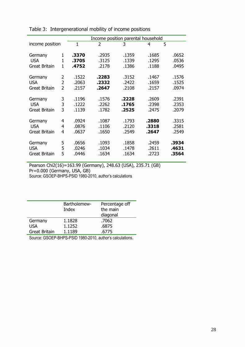
5.2 Intergenerational Income Transitions

The Bartholomew index documents a higher intergenerational income mobility in

Germany compared with Great Britain and the United States. The higher

intergenerational income mobility at the lower end of the income distribution in

17

Germany than in Great Britain and the United States might indicate that social policy,

institutional labor market settings, and the public financed educational system in

Germany succeed to contribute to a higher economic mobility and social permeability

in the society. In the United States, the intergenerational immobility on the top of

the income distribution is more pronounced than in Germany and Great Britain,

which indicates a positive correlation between the children’s economic success and

the parental economic resources: high income parents are able to invest in the

human capital of their children, which guarantees their economic and social

advancement. However, the degree of immobility at the top and at the bottom of the

income distribution might be exaggerated, for upward mobility is not possible for

those performing the highest income category, and downward mobility is not

possible for persons in the lowest income category (Lentz et al. 1989, Mazumdar

2005) (Table 3).

[Table 3 near here]

5.3 Relative Risk of Poverty

Table 4 presents the relative risk ratios (exp(Bc)) and the significance level for each

of the explanatory variables Xc of the binomial logit model. In Germany and the

United States women experience a significant higher probability to count among the

poor than men. In all the countries, each additional child living in the household

significantly increases the relative risk of poverty. In the United States, the own and

parental educational attainment significantly reduces the relative risk of poverty. In

Germany and Great Britain, to hold an academic or a professional occupation

significantly lowers one’s relative risk of poverty. Persons engaged in trade and

service occupations experience a significantly higher probability to count among the

poor. The significant effect of the parental occupational status on the relative poverty

risk underlines the intergenerational class persistence (Lentz and Laband 1989,

Hellerstein and Sandler Morill 2011). In Germany and the United States persons whose

parents are engaged in professional occupations have a significantly lower relative

risk to be poor and persons with parents in elementary professions experience a

significantly higher relative risk of poverty. In Germany, parental unemployment and

18

health dissatisfaction significantly increase the relative poverty risk. In the United

States and Great Britain marital status matters: divorce and separation increase the

relative poverty risk.

[Table 4 near here]

6. Conclusions

We analyzed the extent of and the determinants of intergenerational income mobility

and the relative risk of poverty in Germany, the United States and Great Britain. We

tested from the hypothesis that the country differences concerning the welfare-state

regimes, the family role patterns, the institutional settings of the labor markets, and

the social policy design induce a different working of the individual and parental

socio-economic resources and social exclusion attributes on the intergenerational

income mobility and the relative risk of poverty. The empirical findings partly support

these hypotheses:

- Though similar in their welfare state regime, the United States and Great Britain

differ concerning the average intergenerational income elasticity, the

intergenerational transition of income positions, the impact of individual and

family background characteristics and social exclusion attributes on the

intergenerational income mobility, and the relative risk of poverty.

- In the United States the results show a higher intergenerational correlation of

social and economic status than in Germany and Great Britain, which contradicts

the hypothesis of a mobile society, and a high permeability of the social system.

The intergenerational income immobility is higher than in Great Britain and in

Germany, especially at the top of the income distribution. The inclusion of

individual and family background variables lower the ‘raw’ intergenerational

income elasticity by about one third, compared to about one fourth in Germany,

and about 15 percent in Great Britain. The inclusion of social exclusion attributes

(family disruption, disability and health dissatisfaction) lower the “raw

19

intergenerational income elasticity to a higher extent than in Germany and Great

Britain.

- In Germany, the results reflect two opposing effects: the hypothesized higher

intergenerational social cohesion due to tax policy incentives for traditional family

role patterns may be partly set off by the redistribution effects of social policy.

The German social policy obviously more effectively alleviates the negative impact

of social exclusion attributes on the intergenerational transmission of social and

economic disadvantages than in the United States and in Great Britain.

- The highest intergenerational income persistence is evident in the tails of the

income distribution which corroborates the results of previous studies (Atkinson

et. al. 1983, Dearden et. al. 1997, Corcoran 2001). These results indicate a high

class persistence, an increasing intergenerational transmission of poverty and

social exclusion, a deepening of economic and social inequality across generations

which produces economic inefficiencies imposing economic and social costs.

In general, growing up in poverty or in a social exclusion environment negatively

affects a person’s future social and economic position and life chances. The social

and welfare policies of a country are forced to design efficient policy measures to

break the intergenerational transmission of disadvantages, and to prevent the

development of a self-replicating underclass. Regardless of a country’s welfare state

regime, it is necessary to recognize the potential of education, and to encourage

human capital accumulation to be means to advance the social ladder. However, the

results call for broader analysis of the mechanisms how families, labor markets and

social policy interact in determining the intergenerational transmission of economic

and social (dis-)advantages in further research.

References

Aaronson, D. and Mazumder, D. (2008). Intergenerational Economic Mobility in the

United States, 1940 to 2000. Journal of Human Resources 43,1: 139-172.

20

Acemoglu, D. and Pischke, J.-S. (2000). Changes in the Wage Structure, Family Income, and Children’s Education. NBER Working Paper Series 7986, http://www.nber.org/papers/w7986. Cambridge: NBER.

Arts, W. and Gelissen, J. (2002) . Three worlds of welfare capitalism or more? A state-of-the-art report. Journal of European Social Policy 12: 137-158.

Atkinson, A.B., Maynard, A.K. and Trinder, C.G. (1983). Parents and Children: Incomes in Two Generations. London: Heinemann.

Atkinson, A.B. (1998). Social Exclusion, Poverty and Unemployment. In: J. Hills (ed.) Exclusion, Employment and Opportunity, Centre for Analysis of Social Exclusion (CASE). London: London School of Economics and Political Science.

Bartholemew, D.J. (1982). .Stochastic Models for Social Processes. 3rd ed.. Chichester, UK: Wiley.

Becker, G.S. (1964). Human Capital. New York: NBER. Becker, G.S. and Tomes, N. (1986). Child endowments and the Quantity and Quality

of Children. Journal of Political Economy 84: S143-S1162. Björklund, A. and Jäntti, M. (2000). Intergenerational Mobility of Economic Status in

Comparative Perspective. Nordic Journal of Political Economy 26: 3-32. Blanden, J.P. and Machin, P.G. (2005). Educational Inequality and Intergenerational

Mobility. In: Machin, S. and Vignoes, A. (eds.), What’s the Good of Education? The Economics of Education in the United Kingdom. Princeton: Princeton University Press.

Bonoli, G. (1997). Classifying welfare states: a two-dimension approach. Journal of Social Policy 26(3): 351-372.

Bourguignon, F. and Chakravarty, S. (2003). The Measurement of Multidimensional Poverty. Journal of Economic Inequality 1: 25-49.

Burchard, T., Le Grand, J. and Piachaud, D. (2002), Social exclusion in Britain 1991-1995. Social Policy and Administration 33(3): 227-244.

Castles, F.G. and Mitchell, D. (1993). Worlds of welfare and families of nations. In: Castles, F.G. (ed.), Families of Nations: Patterns of Public Policy in Western Democracies. Aldershot: Dartmouth.

Chadwick, L. and Solon, G. (2002). ‘Intergenerational income mobility among daughters. American Economic Review 92(1): 335-344.

Charles, M., Buchmann, M., Halebsky, S., Powers, J.M. and Smith, M.M. (2001). The context of women’s market careers. Work and Occupations 28: 371-396.

Corcoran, M. (2001). Mobility, Persistence, and the Consequences of Poverty for Children: Child and Adult Outcomes. In: Danziger, S. and Haveman, R. (eds.), Understanding Poverty. Cambridge: Harvard University Press.

Couch, K.A. and Dunn, T. A. (1997). Intergenerational Correlation in Labour Market Status, a Comparison of the United States and Germany. Journal of Human Resources 32(4): 210-232.

Couch, K.A. and Lillard, D.R. (2004). Non-linear patterns in Germany and the United States. In: Corak, M. (ed.), Generational Income Mobility in North America and Europe. Cambridge: Cambridge University Press.

De Swaan, A. (1988). In Care of the State; Health care, education and welfare in Europe and the USA in the Modern Era. Oxford: Oxford University Press.

Dearden, L., Machin, S. and Reed, H. (1997). Intergenerational Mobility in Britain. Economic Journal 107: 46-66.

Duffy, K. (1995). Social Exclusion and Human Dignity in Europe. Strasbourg: Council of Europe.

21

Dustmann, C. (2004). Parental background, secondary school, track choice, and wages. Oxford Economic Papers 56: 209-230.

Erikson R. and Goldthorpe, J.H. (1992a). The Constant Flux: A Study of Class Mobility in Industrial Societies. Oxford: Clarendon Press, Oxford.

Erikson R. and Goldthorpe, J.H. (1992b). Intergenerational Inequality: A Sociological Perspective. Journal of Economic Perspectives 16: 31-44.

Esping-Andersen, G. (1990). The three worlds of welfare capitalism. Cambridge, Oxford: Polity Press.

Esping-Andersen, G. (1994). Welfare States and the Economy. In: Smelser, N.J. and Swedberg, R. (eds.), The Handbook of Economic Sociology. Cambridge, Oxford: Polity Press.

Esping-Andersen, G. (1999). Social foundations of postindustrial economies. Oxford: Oxford University Press.

Finnie, R. and Sweetman, A. (2003). Poverty Dynamics: Empirical Evidence for Canada. Canadian Journal of Economics 36: 291-325.

Fitzgerald, J.M., Gottschalk, P. and Moffitt, R. (1998a). An analysis of the impact of sample attrition in panel data: the Michigan Panel Study of Income Dynamics. Journal of Human Resources 33: 251-299.

Fitzgerald, J.M., Gottschalk, P. and Moffitt, R. (1998b). An analysis of the impact of sample attrition in panel data: the Michigan Panel Study of Income Dynamics. Journal of Human Resources 33: 300-344.

Formby, J.P., Smith, W.J. and Zheng, B. (2004). Mobility measurement, transition matrices and statistical inference. Journal of Econometrics 120: 181-205.

Frick, J.R. and Grabka, M.M. (2005). Item-non-response on income questions in panel surveys: incidence, imputation and the impact on inequality and mobility. Allgemeines Statistisches Archiv 89: 49-61.

Frick, J.R., Jenkins S.P., Lillard, D.R., Lipps, O. and Wooden, M. (2007). The Cross-National Equivalent File (CNEF) and its Member Country Household Panel Studies. Schmollers Jahrbuch (Journal of Applied Social Science Studies) 127(4): 627-654.

Goldthorpe, J.H. (1987). Social Mobility and Class Structure in Modern Britain. Oxford: Clarendon Press.

Goldthorpe, J.H. (2000). Social Class and the Differentiation of Employment Contracts. In: Goldthorpe, J.H. (ed.), On Sociology. Numbers, Narratives, and the Integration of Research and Theory. Oxford: Oxford University Press.

Ganzeboom, H.B.G., De Graaf, P., Treimann, D.J. and De Leeuw, J. (1992). A Standard International Socio-Economic Index of Occupational Status. Social Science Research 21(1): 1-56.

Ganzeboom, H.B.G. and Treimann, D.J. (1996). Internationally Measures of Occupational Status for the 1988 International Standard Classification of Occupations. Social Science Research 25: 201-239.

Ganzeboom, H.B.G. and Treimann, D.J. (2003). Three Internationally Standardised Measures for Comparative Research on Occupational Status. In: Hoffmeyer-Zlotnik, J.H.P. and Wolf, C. (eds.) Advances in Cross-national Comparison. A European Working Book for Demographic and Socio-Economic Variables. New York: Kluwer Academic Press.

22

Gornick, J.C. and Meyers, M.K. (2003). Families that work – Policies for Reconciling Parenthood and Employment. New York: Russel Sage Foundation.

Grawe, N.D. (2004). Reconsidering the Use of Nonlinearities in Intergenerational Earnings Mobility as a Test for Credit Constraints. Journal of Human Resources 39: 813-827.

Hagenaars, A.J. M., de Vos, K. and Zaidi, M.A. (1994). Poverty Statistics in the Late 1980s: Research Based on Micro-data. Luxembourg: Office for Official Publications of the European Communities.

Hall, P.A. and Soskice, D. (2001). Varieties of Capitalism. An Introduction to the Varieties of Capitalism. In: P.A. Hall and D. Soskice (eds.), Varieties of Capitalism: The Institutional Foundations of Comparative Advantage. Oxford/New York: Oxford University Press, 71-103.

Heckman, J.J. (1981). Statistical models for discrete panel data’, in: Manski, C.F. and McFadden, D. (eds.) Structural Analysis of Discrete Data with Econometric Applications. Cambridge: MIT Press, Cambridge.

Hellerstein, J.K. and Sandler Morill, M. (2011). Dads and Daughters. The Changing Impact of Fathers on Women’s Occupational Choices. Journal of Human Resources 46(2): 333-372.

Hertz, T. (2004). Rags, riches and race: The intergenerational economic mobility of black and white families in the United States. In: Bowles, S., Gintis, H. and Osborne, M. (eds.) Unequal chances: Family background and economic success. Princeton: Princeton University Press.

Howarth, C., Kenway, P., Palmer, G. and Street, C. (1998). Monitoring Poverty and Social Exclusion: Labour’s Inheritance. New York: New Policy Institute, Joseph Rowntree Foundation.

International Labor Office (ILO) (1990). ISCO-88: International Standard Classification of Occupations. Geneva: ILO.

Kautto, M. (2002). Investing in services in West European welfare states. Journal of European Social Policy 12(1): 53-65.

Korpi, W. and Palme, J. (1998). The paradox of redistribution and the strategy of equality: welfare state institutions, inequality and poverty in the Western countries. American Sociological Review 63: 662-687.

Lee, C.-I. and Solon, G. (2009). Trends in intergenerational income mobility. The Review of Economics and Statistics 91,4: 766-772.

Leibfried, S. (1992). Towards a European welfare state. In: Ferge, Z. and Kolberg, I.E. (eds.) Social Policy in a Changing Europe. Frankfurt: Campus.

Lentz, B.F. and Laband, D.N. (1989). Why So Many Children of Doctors Become Doctors: Nepotism vs. Human Capital Transfers. Journal of Human Resources 24(3): 396-413.

Levitas, R., Pantazis, C., Fahmy, E., Gordon, D., Lloyd, E. and Patsios, D. (2007). The multi-dimensional analysis of social exclusion. Bristol: Department of Sociology and School for Social Policy, University of Bristol.

Lewis, J. (2006). Work/family reconciliation, equal opportunities and social policies: the interpretation of policy trajectories at the EU level and the meaning of gender equality. Journal of European Public Policy 13(3): 420-437.

23

Maddala, G.S. (1983). Limited-Dependent and Qualitative Variables in Econometrics. Cambridge: Cambridge University Press.

Marlier, E. and Atkinson, A.B. (2010). Indicators of Poverty and Social Exclusion in a Global Context. Journal of Policy Analysis and Management 29: 285-304.

Mayer, S.E. (1997). What Money Can’t Buy: Family Income and Children’s Life Chances. Cambridge: Harvard University Press.

Mayer, S.E. and Lopoo, L.M (2005). Has the Intergenerational Transmission of Economic Status Changed?. The Journal of Human Resources 40(1): 169-185.

Mayer, S.E. and Lopoo, L.M. (2008). Government spending and intergenerational mobility. Journal of Public Economics 92(1-2): 139-158.

Mazumdar, B. (2005). Fortunate Sons: New estimated of Intergenerational Mobility in the United States using Social Security Earnings Data. The Review of Economics and Statistics 87: 235-255.

McFadden, D. (1973). Conditional Logit Analysis of Qualitative Choice Behavior. In: Zarembka, P. (ed.) Frontiers of econometrics. New York: Academic Press.

Mincer, J. (1974). Schooling, Experience and Earnings. New York: NBER.

Mortimer, J.T. and Krüger, H. (2000). Transitions from School to Work in the United States and Germany: Formal Pathways Matter. In: M. Hallinan (ed.), Handbook of the Sociology of Education. New York, 475-497.

Navarro, V. and Shi, L. (2001). The political context of social inequalities. Journal of Health Services 31: 1-21.

OECD (1982). The OECD List of Social Indicators. Paris: OECD. OECD (2012). Education at a Glance 2012. OECD Indicators, OECD Publishing. Pencavel, J. (1998). Assortative Mating by Schooling and the Work Behavior of Wives

and Husbands. American Economic Review 88(2): 326-329. Saunders, P. (2008). Measuring wellbeing using non-monetary indicators:

Deprivation and social exclusion. Family Matters 78: 8-17. Saunders, P., Naidoo, Y. and Griffiths, M. (2007). Towards new indicators of

disadvantage: Deprivation and social exclusion in Australia. Sydney: Social Policy Research Centre.

Sen, A.K. (1985). Commodities and Capabilities. Amsterdam: North-Holland. Sen, A.K. (1992). Inequality Re-examined. Oxford: Clarendon Press. SEU (Social Exclusion Unit) (1997). Social Exclusion Unit: Purpose, work priorities

and working methods. London: Cabinet Office. Shorrocks, A. F. (1978). The measurement of mobility. Econometrica 46: 1013-

1024. Siaroff, A. (1994). Work, welfare and gender equality: a new typology. In: Sainsbury,

D. (ed.) Gendering Welfare States. London: Sage.

Solon, G. (1992). Intergenerational Income Mobility in the United States. American Economic Review 82(3): 326-329.

Solon, G. (1999). Intergenerational Mobility in the Labor Market. In: Ashenfelter, O. and Card, D. (eds.) Handbook of Labor Economics. Amsterdam: North Holland.

Solon, G. (2002). Cross-Country Differences in Intergenerational Earnings Mobility. Journal of Economic Perspectives 16: 59-66.

24

Solon, G. (2004). A Model of Intergenerational Mobility Variation over Time and Place. In: Corak, M. (ed.), Generational Income Mobility in North America and Europe. Amsterdam: North Holland.

Stevens, A.H. (1999). Climbing Out of Poverty. Falling Back In: Measuring the Persistence of Poverty over Multiple Spells. Journal of Human Resources 34: 557-588.

Therborn, G. (1995). European Modernity and Beyond. The Trajectory of European Societies 1945-2000. London: Sage Publications.

Townsend, P. (1979). Poverty in the United Kingdom. Harmondsworth: Penguin. United Nations (1995). The Copenhagen Declaration and Programme of Action:

World Summit for Social Development 6-12 March 1995. New York: UN Department of Publications.

25

Tables

26

Table 1: Descriptive statistics

Variables Description Germany United States Great Britain

Mean / % in 1 SD Mean/ % in 1 SD Mean/ % in 1 SD

y

ln(permanent real equivalent post-government income (2001=100, OECD equivalence scale, 5-year average)

9.564 .491 9.835 .930 9.311 .466

yP

ln(permanent real equivalent post-government income (2001=100, OECD equivalence scale, 5-year average), parental household

9.380 .388 9.445 .659 8.984 .447

GEN 1 male, 0 female .5202 .4887 .5136

EDUC Educational attainment, school years 12.442 2.916 12.807 2.030 n.a.

EDUCP Educational attainment parents, average years of education 10.521 1.971 12.446 1.851 n.a.

CHILD Number of children in the household 1.128 1.052 1.412 1.278 1.246 1.211

EMPP 1 father/mother is employed less than half the observation period, 0 else .2093 .2830 .2335

OCC Occupational categories

1 “1 academic/scientific professions/managers”, 0 else

1 “2 professionals/technicians/ associate professionals”, 0 else

1 “3 trade/personal service”, 0 else

1 “7 elementary occupations”, 0 else

.4632

.2538

.1028

.1802

.3405

.1916

.2211

.1562

.3933

.2826

.1101

.1334

OCCp

Occupational categories (father/mother)

1 “1 academic/scientific professions/managers”, 0 else

1 “2 professionals/technicians/ associate professionals”, 0 else

1 “3 trade/personal service”, 0 else

1 “7 elementary occupations”, 0 else

.3144

.2085

.1070

.1572

.3721

.1878

.1259

.2387

.3211

.2473

.1634

.1820

DISRUPT Family disruption : 1 widowed, divorced, separated, 0 else .0903 .0952 .0678

DISRUPTP Family disruption, father/mother: 1 widowed, divorced, separated, 0 else .1775 .2669 .2103

DISABIL Disability status: 1 disabled, 0 else .0862 .0712 .0272

DISABILP Disability status, father/ mother: 1 disabled, 0 else .0519 .0809 .0804

SATHEALTHP Dissatisfaction with health, father/mother: 1 poor, very poor , 0 else .1693 .1358 .0801

N Number of observations 2,128 2,585 1,840

Source: Source: GSOEP-BHPS-PSID 1980-2010, author’s calculations. Note: The subscripts indicates the parental household characteristics in double parents’ families the variable refers to the father, in single parents households to the father or the mother.

27

Table 2: Intergenerational income elasticities

Model specification

Description

(a) (b) (c)

Germany USA GB Germany USA GB Germany USA GB

Constant

5.002***

3.346*** 4.779*** 6.181*** 4.647*** 5.595*** 6.312*** 5.579*** 6.021***

yp post-gvt income, parental hh .484***

.678***

.504*** .377*** .465*** .426*** .374*** .385*** .400***

2X GEN 1 male 0 female -.149*** -.128*** -.031 -.123*** -.120*** -.028

3X EDUC .017*** .088*** n.a. .019*** .087*** n.a.

4X CHILD -.149*** -.171*** -.127*** -.162*** -.197*** -.133**

5X EDUCp .004 .009 n.a. .005 .003 n.a.

6X OCCp 1 academic/scientific/managers, 0 else 1 professionals, 0 else 1 trade/personal service, 0 else 1 elementary occupations, 0 else

.126*

.087

.004 -.121

.084

.069

.008 -.074

.207***

.214*** .070 .019

.144* .099 .013 -.114

.048 .044 .020 -.103

.212*** .212*** .078 .111

7X EMPp 1 unemployed, 0 else -.031 -.055 -.021

8X DISRUPT 1 family disruption, 0 else -.162** -.322*** -.019

9X DISRUPTp 1 family disruption, 0 else .089 .089 .089

10X DISABILITYp 1 disabled, 0 else -.219* -.003 -.129

11X DISABILITY 1 disabled, 0 else -.081 -.447*** -.068

12X SATHEALTHp 1 excellent, good, fair; 0 poor, very poor

-.119 -.190 -.138

R2adj .130 .229 .219 .356 .289 .323 .394 .365 .328 RMSE .458 .815 .411 .347 .708 .355 .338 .651 .354 LL -584 -1310 -537 -120 -790 -149 -106 -686 -145 Mean VIF 1.23 1.30 1.30 1.23 1.30 1.30 1.23 1.30 1.30 N 919 1079 1014 347 741 400 341 702 399

Source: GSOEP-BHPS-PSID 1980-2010, author’s calculations. NOTE: * p<0.05; ** p<0.01; *** p<0.001

28

Table 3: Intergenerational mobility of income positions

income position

Income position parental household 1 2 3 4 5

Germany 1 .3370 .2935 .1359 .1685 .0652 USA 1 .3705 .3125 .1339 .1295 .0536 Great Britain 1 .4752 .2178 .1386 .1188 .0495 Germany 2 .1522 .2283 .3152 .1467 .1576 USA 2 .2063 .2332 .2422 .1659 .1525 Great Britain 2 .2157 .2647 .2108 .2157 .0974 Germany 3 .1196 .1576 .2228 .2609 .2391 USA 3 .1222 .2262 .1765 .2398 .2353 Great Britain 3 .1139 .1782 .2525 .2475 .2079 Germany 4 .0924 .1087 .1793 .2880 .3315 USA 4 .0876 .1106 .2120 .3318 .2581 Great Britain 4 .0637 .1650 .2549 .2647 .2549 Germany 5 .0656 .1093 .1858 .2459 .3934 USA 5 .0246 .1034 .1478 .2611 .4631 Great Britain 5 .0446 .1634 .1634 .2723 .3564

Pearson Chi2(16)=163.99 (Germany), 248.63 (USA), 235.71 (GB) Pr=0.000 (Germany, USA, GB) Source: GSOEP-BHPS-PSID 1980-2010, author’s calculations

Bartholemew-Index

Percentage off the main diagonal

Germany 1.1828 .7062 USA 1.1252 .6875 Great Britain 1.1189 .6775

Source: GSOEP-BHPS-PSID 1980-2010, author’s calculations.

29

Table 4: The Relative Risk of Poverty

Germany

USA

GB

GEN 1 male 0 female 2.365* 1.863* .879 EDUC .989 .627* n.a. CHILD 2.457* 2.082* 2.499* OCC 1 academic/scientific/managers, 0 else 1 professionals, 0 else 1 trade/personal service, 0 else 1 elementary occupations, 0 else

1.148* 1.249* .887 .099

1.811 1.094 3.029** .106

1.396* 1.231* 1.716 .115

EDUCP .989 .967* n.a. OCCP 1 academic/scientific/managers, 0 else 1 professionals, 0 else 1 trade/personal service, 0 else 1 elementary occupations, 0 else

1.115* 1.905 .999 .364*

1.333 1.004 .996 .996*

.499 1.344* .896 1.685

EMPP 1 unemployed, 0 else .166* .796 .544 DISRUPT 1 family disruption, 0 else .566 .808*** .805* DISRUPTP 1 family disruption, 0 else .891 .824 .972 DISABILITY 1 disabled, 0 else .277 .865 .216 SATHEALTHP 1 excellent, good, fair; 0 poor, very poor

3.287* .841 1.364

L -111.262 -252.429 -148.281

2χ 97.79 139.59 99.19

Pseudo R2 .3053 .2166 .2506 N 257 517 335 Source: GSOEP-BHPS-PSID 1980-2010, author’s calculations. NOTE: * p<0.05; ** p<0.01; *** p<0.001