the intuitive guide to fourier analysis and spectral...
TRANSCRIPT
The Intuitive Guide to
Fourier Analysis and Spectral Estimation
Charan Langton
Victor Levin
Academic
Mountcastle Academic
The Intuitive Guide to Fourier Analysis and Spectral Estimation
©Charan Langton, Victor Levin, 2016All Rights Reserved
Thank you for buying The Intuitive Guide to Fourier Analysis and Spectral Estimation. By respectingour copyright, you are helping independent authors and publishers benefit from their contributionto the world of knowledge. We thank you for complying with the copyright provisions by nottransmitting, reproducing, scanning, or distributing any part of this book without permission of thepublisher. By doing so, you are helping us to keep writing and producing valuable content for youand others. If you would like to use any part of this text for academic purposes, please do contact usfor permission. Thank you.
The authors gratefully acknowledge so many websites, that freely share their knowledge on theInternet, making this a rich world to both showcase our work and to learn from others.
www.complextoreal.com/fftguideMATLAB code and other supplemental material will be available at this website.
The Library of Congress cataloging data has been applied for.
ISBN-13: eBook: 9780913063262ISBN-10: eBook: 09130632661. Fourier transform 2. Signal processing 3. Stochastic signal analysis 4. Spectral estimation
First eBook Edition, August 20161 2 3 4 5 6Printed in the United States of America
Book cover design by Josep BlancoBook interior design and Latex typesetting by Patricio PradaEditing by Grima Sharma
2

Contents
Preface vii
1 Trigonometric Representation of CT Periodic Signals 1What is Fourier Analysis . . . . . . . . . . . . . . . . . . . . . . . . . . . . . . . . . . . . . 2Frequency and Time Domain Views of a Signal . . . . . . . . . . . . . . . . . . . . . . . 4
Spectrum of a signal . . . . . . . . . . . . . . . . . . . . . . . . . . . . . . . . . . . . 4Fundamental waves and their harmonics . . . . . . . . . . . . . . . . . . . . . . . . 6
Harmonics as Basis Functions . . . . . . . . . . . . . . . . . . . . . . . . . . . . . . . . . . 10Evenness and oddness of sinusoids . . . . . . . . . . . . . . . . . . . . . . . . . . . 11Making waves . . . . . . . . . . . . . . . . . . . . . . . . . . . . . . . . . . . . . . . . 12Square waves . . . . . . . . . . . . . . . . . . . . . . . . . . . . . . . . . . . . . . . . 12Gibbs phenomenon . . . . . . . . . . . . . . . . . . . . . . . . . . . . . . . . . . . . . 15Creating a sawtooth wave . . . . . . . . . . . . . . . . . . . . . . . . . . . . . . . . . 15
Generalizing the Fourier Series Equation . . . . . . . . . . . . . . . . . . . . . . . . . . . 16Multiple ways of writing the Fourier series equation . . . . . . . . . . . . . . . . . 17Fourier series in complex exponential form . . . . . . . . . . . . . . . . . . . . . . 18
The Fourier Analysis . . . . . . . . . . . . . . . . . . . . . . . . . . . . . . . . . . . . . . . . 19Computing a0, the DC coefficient . . . . . . . . . . . . . . . . . . . . . . . . . . . . 19Computing bk, the coefficients of sine harmonics . . . . . . . . . . . . . . . . . . . 21Computing ak, the coefficients of cosine harmonics . . . . . . . . . . . . . . . . . 25Coefficients become the spectrum . . . . . . . . . . . . . . . . . . . . . . . . . . . . 29The power spectrum . . . . . . . . . . . . . . . . . . . . . . . . . . . . . . . . . . . . 32
2 Complex Representation of Continuous-Time Periodic Signals 37Euler’s Equation . . . . . . . . . . . . . . . . . . . . . . . . . . . . . . . . . . . . . . . . . . 38
The complex exponential . . . . . . . . . . . . . . . . . . . . . . . . . . . . . . . . . 38Projections of a complex exponential . . . . . . . . . . . . . . . . . . . . . . . . . . 40
i
CONTENTS
The Sinusoids . . . . . . . . . . . . . . . . . . . . . . . . . . . . . . . . . . . . . . . . . . . . 42Fourier Series Representation using Complex Exponentials . . . . . . . . . . . . . . . . 45
Double-sided spectrum . . . . . . . . . . . . . . . . . . . . . . . . . . . . . . . . . . . 50Power spectrum . . . . . . . . . . . . . . . . . . . . . . . . . . . . . . . . . . . . . . . 58
Appendix: A little bit about complex numbers . . . . . . . . . . . . . . . . . . . . . . . . 64
3 Discrete-Time Signals and Fourier Series Representation 69Fourier Series and Discrete-time Signals . . . . . . . . . . . . . . . . . . . . . . . . . . . 70
Discrete signals are different . . . . . . . . . . . . . . . . . . . . . . . . . . . . . . . 70Discrete vs. digital . . . . . . . . . . . . . . . . . . . . . . . . . . . . . . . . . . . . . 70Generating discrete signals . . . . . . . . . . . . . . . . . . . . . . . . . . . . . . . . 71
Sampling and Interpolation . . . . . . . . . . . . . . . . . . . . . . . . . . . . . . . . . . . 72Ideal sampling . . . . . . . . . . . . . . . . . . . . . . . . . . . . . . . . . . . . . . . . 72Reconstruction of an analog signal from discrete samples . . . . . . . . . . . . . 73Method 1: Zero-Order-Hold . . . . . . . . . . . . . . . . . . . . . . . . . . . . . . . 75Method 2: First-Order-Hold (linear interpolation) . . . . . . . . . . . . . . . . . . 76Method 3: Sinc interpolation . . . . . . . . . . . . . . . . . . . . . . . . . . . . . . . 77Sinc function detour . . . . . . . . . . . . . . . . . . . . . . . . . . . . . . . . . . . . 78Sampling rate . . . . . . . . . . . . . . . . . . . . . . . . . . . . . . . . . . . . . . . . 81
Shannon’s Theorem . . . . . . . . . . . . . . . . . . . . . . . . . . . . . . . . . . . . . . . . 81Aliasing of discrete signals . . . . . . . . . . . . . . . . . . . . . . . . . . . . . . . . 83Bad sampling . . . . . . . . . . . . . . . . . . . . . . . . . . . . . . . . . . . . . . . . . 83Good sampling . . . . . . . . . . . . . . . . . . . . . . . . . . . . . . . . . . . . . . . . 85
Discrete Signal Parameters . . . . . . . . . . . . . . . . . . . . . . . . . . . . . . . . . . . . 87Digital frequency, only for discrete signals . . . . . . . . . . . . . . . . . . . . . . . 88Are discrete signals periodic? . . . . . . . . . . . . . . . . . . . . . . . . . . . . . . . 90
Discrete Complex Exponentials as Basis of DT Fourier Series . . . . . . . . . . . . . . . 92Harmonics of a discrete fundamental CE . . . . . . . . . . . . . . . . . . . . . . . . 93Repeating harmonics of a discrete signal . . . . . . . . . . . . . . . . . . . . . . . . 93
Discrete-Time Fourier Series Representation . . . . . . . . . . . . . . . . . . . . . . . . . 98DTFS Examples . . . . . . . . . . . . . . . . . . . . . . . . . . . . . . . . . . . . . . . 99DTFSC of a repeating square pulse signal . . . . . . . . . . . . . . . . . . . . . . . 105
Power spectrum . . . . . . . . . . . . . . . . . . . . . . . . . . . . . . . . . . . . . . . . . . 109Matrix method for computing FSC . . . . . . . . . . . . . . . . . . . . . . . . . . . . . . . 109
4 Fourier Transform of aperiodic and periodic signals 115Applying Fourier Series to Aperiodic Signals . . . . . . . . . . . . . . . . . . . . . . . . . 116
ii

CONTENTS
Extending the period to infinity . . . . . . . . . . . . . . . . . . . . . . . . . . . . . 116Continuous-Time Fourier Transform . . . . . . . . . . . . . . . . . . . . . . . . . . . 118
Comparing FSC and the Fourier Transform . . . . . . . . . . . . . . . . . . . . . . . . . . 121CTFT of Important Aperiodic Functions . . . . . . . . . . . . . . . . . . . . . . . . . . . . 123
CTFT of an impulse function . . . . . . . . . . . . . . . . . . . . . . . . . . . . . . . 123CTFT of a constant . . . . . . . . . . . . . . . . . . . . . . . . . . . . . . . . . . . . . 126CTFT of a sinusoid . . . . . . . . . . . . . . . . . . . . . . . . . . . . . . . . . . . . . 127CTFT of a complex exponential . . . . . . . . . . . . . . . . . . . . . . . . . . . . . 128Time-shifting a function . . . . . . . . . . . . . . . . . . . . . . . . . . . . . . . . . . 130Duality with frequency shift . . . . . . . . . . . . . . . . . . . . . . . . . . . . . . . . 132Convolution property . . . . . . . . . . . . . . . . . . . . . . . . . . . . . . . . . . . . 133CTFT of a Gaussian function . . . . . . . . . . . . . . . . . . . . . . . . . . . . . . . 135CTFT of a square pulse . . . . . . . . . . . . . . . . . . . . . . . . . . . . . . . . . . . 136
Fourier Transform of Periodic Signals . . . . . . . . . . . . . . . . . . . . . . . . . . . . . 138CTFT of a periodic square pulse train . . . . . . . . . . . . . . . . . . . . . . . . . . 140
5 DT Fourier Transform of Aperiodic and Periodic Signals 147Discrete Time Fourier Transform . . . . . . . . . . . . . . . . . . . . . . . . . . . . . . . . 149DTFT of aperiodic signals . . . . . . . . . . . . . . . . . . . . . . . . . . . . . . . . . . . . 150
Comparing DTFT with CTFT . . . . . . . . . . . . . . . . . . . . . . . . . . . . . . . 151Obtaining a DTFT from CTFT . . . . . . . . . . . . . . . . . . . . . . . . . . . . . . . 152DTFT of a delayed impulse . . . . . . . . . . . . . . . . . . . . . . . . . . . . . . . . 153DTFT of superposition of impulses . . . . . . . . . . . . . . . . . . . . . . . . . . . . 154DTFT of a square pulse . . . . . . . . . . . . . . . . . . . . . . . . . . . . . . . . . . . 156Dirichlet detour . . . . . . . . . . . . . . . . . . . . . . . . . . . . . . . . . . . . . . . 158Applying time-shift property to the DTFT of a square pulse . . . . . . . . . . . . 160Time expansion property . . . . . . . . . . . . . . . . . . . . . . . . . . . . . . . . . 160DTFT of a triangular pulse . . . . . . . . . . . . . . . . . . . . . . . . . . . . . . . . 162DTFT of a raised-cosine pulse . . . . . . . . . . . . . . . . . . . . . . . . . . . . . . . 163DTFT of a Gaussian pulse . . . . . . . . . . . . . . . . . . . . . . . . . . . . . . . . . 164
DTFT of periodic signals . . . . . . . . . . . . . . . . . . . . . . . . . . . . . . . . . . . . . 165DTFT of important periodic signals . . . . . . . . . . . . . . . . . . . . . . . . . . . 168
6 Discrete Fourier Transform 175Four Cases of Fourier Transform . . . . . . . . . . . . . . . . . . . . . . . . . . . . . . . . 176The Discrete Fourier Transform . . . . . . . . . . . . . . . . . . . . . . . . . . . . . . . . 178
DFT from DTFT . . . . . . . . . . . . . . . . . . . . . . . . . . . . . . . . . . . . . . . 178
iii
CONTENTS
DFT frequency resolution . . . . . . . . . . . . . . . . . . . . . . . . . . . . . . . . . 179Understanding the X-axis of a DFT . . . . . . . . . . . . . . . . . . . . . . . . . . . . 181Periodic signal assumption . . . . . . . . . . . . . . . . . . . . . . . . . . . . . . . . 182
Computing DFT . . . . . . . . . . . . . . . . . . . . . . . . . . . . . . . . . . . . . . . . . . 183Computing DFT, the hard way with integration . . . . . . . . . . . . . . . . . . . . 183Computing DFT, the easier way with matrix math . . . . . . . . . . . . . . . . . . 186
Computing DFT, the Easy Way With Matlab . . . . . . . . . . . . . . . . . . . . . . . . . 191Zero-padding . . . . . . . . . . . . . . . . . . . . . . . . . . . . . . . . . . . . . . . . . . . . 192
Better interpolation density vs. better resolution . . . . . . . . . . . . . . . . . . . 195Fundamental Functions and Their DFT . . . . . . . . . . . . . . . . . . . . . . . . . . . . 196
DFT of an impulse function . . . . . . . . . . . . . . . . . . . . . . . . . . . . . . . . 196DFT of a delayed impulse . . . . . . . . . . . . . . . . . . . . . . . . . . . . . . . . . 197DFT of a sinusoid . . . . . . . . . . . . . . . . . . . . . . . . . . . . . . . . . . . . . . 197DFT of a complex exponential . . . . . . . . . . . . . . . . . . . . . . . . . . . . . . 197DFT of a square pulse . . . . . . . . . . . . . . . . . . . . . . . . . . . . . . . . . . . 200DFT of a finite sinc function . . . . . . . . . . . . . . . . . . . . . . . . . . . . . . . . 201DFT repeats with sampling frequency . . . . . . . . . . . . . . . . . . . . . . . . . . 202
DFT Periodicity and Leakage . . . . . . . . . . . . . . . . . . . . . . . . . . . . . . . . . . 202Truncation effect . . . . . . . . . . . . . . . . . . . . . . . . . . . . . . . . . . . . . . 204Truncation causes leakage . . . . . . . . . . . . . . . . . . . . . . . . . . . . . . . . . 205Reducing leakage by doing a longer DFT . . . . . . . . . . . . . . . . . . . . . . . . 206Reducing leakage by windowing . . . . . . . . . . . . . . . . . . . . . . . . . . . . . 207
DFT and Multi-rate Processing . . . . . . . . . . . . . . . . . . . . . . . . . . . . . . . . . 209Up-sampling and seeing images . . . . . . . . . . . . . . . . . . . . . . . . . . . . . 209Down-sampling . . . . . . . . . . . . . . . . . . . . . . . . . . . . . . . . . . . . . . . 212Interpolation . . . . . . . . . . . . . . . . . . . . . . . . . . . . . . . . . . . . . . . . . 213
Convolution by DFT . . . . . . . . . . . . . . . . . . . . . . . . . . . . . . . . . . . . . . . . 213Short-Time Fourier Transform . . . . . . . . . . . . . . . . . . . . . . . . . . . . . . . . . . 216DFT in Real-Life . . . . . . . . . . . . . . . . . . . . . . . . . . . . . . . . . . . . . . . . . . 217Fast Fourier Transform . . . . . . . . . . . . . . . . . . . . . . . . . . . . . . . . . . . . . . 219
7 Leakage Mitigation with Windows 225Smearing and Leakage Due to Truncation . . . . . . . . . . . . . . . . . . . . . . . . . . 226The Rectangular Truncation Window . . . . . . . . . . . . . . . . . . . . . . . . . . . . . 228
The rectangular window is always present . . . . . . . . . . . . . . . . . . . . . . . 229Window Quality Metrics . . . . . . . . . . . . . . . . . . . . . . . . . . . . . . . . . . . . . 233Filtering with Windows . . . . . . . . . . . . . . . . . . . . . . . . . . . . . . . . . . . . . . 234
iv
CONTENTS
Spectral Estimation . . . . . . . . . . . . . . . . . . . . . . . . . . . . . . . . . . . . . . . . 235Comparing windows . . . . . . . . . . . . . . . . . . . . . . . . . . . . . . . . . . . . 236The Kaiser window . . . . . . . . . . . . . . . . . . . . . . . . . . . . . . . . . . . . . 238
8 Fourier Analysis of Random Signals 245Fourier Analysis of Deterministic vs. Random Signals . . . . . . . . . . . . . . . . . . . 246
Conditions when Fourier analysis is valid . . . . . . . . . . . . . . . . . . . . . . . 247Energy and Power Signals . . . . . . . . . . . . . . . . . . . . . . . . . . . . . . . . . . . . 250
Energy spectral density . . . . . . . . . . . . . . . . . . . . . . . . . . . . . . . . . . . 251Power dpectral density . . . . . . . . . . . . . . . . . . . . . . . . . . . . . . . . . . . 254
Characteristics of Random Signals . . . . . . . . . . . . . . . . . . . . . . . . . . . . . . . 256An ensemble and a realization . . . . . . . . . . . . . . . . . . . . . . . . . . . . . . 257Measure of randomness . . . . . . . . . . . . . . . . . . . . . . . . . . . . . . . . . . 257Stationarity . . . . . . . . . . . . . . . . . . . . . . . . . . . . . . . . . . . . . . . . . . 259Strict and not so strict stationarity . . . . . . . . . . . . . . . . . . . . . . . . . . . . 259Ergodicity . . . . . . . . . . . . . . . . . . . . . . . . . . . . . . . . . . . . . . . . . . . 260
Understanding Properties of Random Signals . . . . . . . . . . . . . . . . . . . . . . . . 262Time average vs. ensemble Average . . . . . . . . . . . . . . . . . . . . . . . . . . . 262Probability distribution . . . . . . . . . . . . . . . . . . . . . . . . . . . . . . . . . . . 263Moments . . . . . . . . . . . . . . . . . . . . . . . . . . . . . . . . . . . . . . . . . . . 265
The Auto-correlation Function . . . . . . . . . . . . . . . . . . . . . . . . . . . . . . . . . 267Ways of looking at ACF . . . . . . . . . . . . . . . . . . . . . . . . . . . . . . . . . . 268Varieties of auto-correlation function . . . . . . . . . . . . . . . . . . . . . . . . . . 268Properties of the ACF . . . . . . . . . . . . . . . . . . . . . . . . . . . . . . . . . . . . 275Comparing auto-correlation with convolution . . . . . . . . . . . . . . . . . . . . . 277
Some Interesting Signals and Their ACF . . . . . . . . . . . . . . . . . . . . . . . . . . . 279Barker codes . . . . . . . . . . . . . . . . . . . . . . . . . . . . . . . . . . . . . . . . . 279Chirp signal . . . . . . . . . . . . . . . . . . . . . . . . . . . . . . . . . . . . . . . . . . 280
Fourier Transform of the ACF . . . . . . . . . . . . . . . . . . . . . . . . . . . . . . . . . . 280
9 Power Spectrum of Random Signals 287Power Spectrum of a Deterministic signal . . . . . . . . . . . . . . . . . . . . . . . . . . 288Spectrum of a Random Signal . . . . . . . . . . . . . . . . . . . . . . . . . . . . . . . . . . 289Nonparametric Spectral Estimation via Autopower . . . . . . . . . . . . . . . . . . . . . 290
ACF bias caused by finite signal length . . . . . . . . . . . . . . . . . . . . . . . . . 291The Measure of an Estimate, MSE, Bias and Variance . . . . . . . . . . . . . . . . . . . 293The Autopower Method and its parameters . . . . . . . . . . . . . . . . . . . . . . . . . 294
v
CONTENTS
What is a reasonable length for the signal? . . . . . . . . . . . . . . . . . . . . . . 295Biased vs. unbiased ACF . . . . . . . . . . . . . . . . . . . . . . . . . . . . . . . . . . 296Windowing the ACF . . . . . . . . . . . . . . . . . . . . . . . . . . . . . . . . . . . . 298How to choose a window . . . . . . . . . . . . . . . . . . . . . . . . . . . . . . . . . 298Shortening the ACF . . . . . . . . . . . . . . . . . . . . . . . . . . . . . . . . . . . . . 299Blackman-Tukey Algorithm to improve the Autopower . . . . . . . . . . . . . . . 301
The Periodogram . . . . . . . . . . . . . . . . . . . . . . . . . . . . . . . . . . . . . . . . . . 302Periodogram vs. length of signal . . . . . . . . . . . . . . . . . . . . . . . . . . . . . 304Improving the Periodogram . . . . . . . . . . . . . . . . . . . . . . . . . . . . . . . . 307Reducing Periodogram variance using the Bartlett Method . . . . . . . . . . . . . 309Reducing Periodogram variance with the Welch Method . . . . . . . . . . . . . . 311Bartlett method . . . . . . . . . . . . . . . . . . . . . . . . . . . . . . . . . . . . . . . 311Welch method . . . . . . . . . . . . . . . . . . . . . . . . . . . . . . . . . . . . . . . . 312
Comparing Autopower and Periodogram . . . . . . . . . . . . . . . . . . . . . . . . . . . 312Figure of Merit of a Spectrum . . . . . . . . . . . . . . . . . . . . . . . . . . . . . . . . . . 313
vi
Preface
The Fourier transform shows up in so many different fields, that there isn’t an another conceptthat spans across so many disciplines. Even the famous Heisenberg uncertainty principle isjust a restating of the Fourier transform. There is no other mathematical concept that givesone as much bang for the buck as does the Fourier analysis. If you have a strong grasp of thisconcept, it can help you solve problems in interference, communications, probability theory,cryptography, acoustics, optics, control systems, and the list goes on. Like e and the goldenratio, it is one of those concepts, which defies boundaries and show up everywhere.
In college, not enough time is devoted to this subject. All electrical engineering studentseither take a Transform theory class or are exposed to it in bits and pieces in a DSP course.In DSP classes, the application of Fourier transform is thrown in with other material suchas linear systems analysis. However, DSP only makes sense when you understand Fourieranalysis well. All fundamental concepts of DSP are based on Fourier analysis. In mathematicsand physics, this subject is covered only cursorily and left as an optional class in othersciences.
This book is intended to give both students and practicing engineers a deeper understandingof Fourier analysis, as a stand-alone topic from its emergence as Fourier series, its applicationto both analog and discrete signals and finally to spectral estimation using the Fourier trans-form. While this subject is at the pinnacle of human achievement, engineering education,due to the limited time available, often fails to impart its beauty and scope to students. Itoften takes years to appreciate this and happens mostly on the job when you have to applythese concepts to something “real.”
Our main goal in this book is to help you fully understand what is happening when youcompute an FFT of a discrete signal. It is intended to deepen your understanding of thetransform theory on which much of numerical analysis is built. There is a whole long storybehind this apparently easy-to-compute but hard-to-understand concept. We start the storywith the Fourier series in its original trigonometric form as imagined by Baron Fourier, and
vii
CONTENTS
then progress through all its developments with contributions from other notables along theway to the end point, the spectral estimation of random signals using the discrete Fouriertransform. In the last two chapters of this book, we cover application of the Fourier analysisto the non-parametric spectral analysis of random signals.
The Fourier transform, a special case of the Laplace transform, is a fundamental tool for theanalysis of stationary signals. In this book, we only cover Fourier analysis and although itleads to all sorts of other important transforms, we feel it is best not to confuse the issue byintroducing other transforms. They all deserve a book of their own.
One of the hardest parts of writing this book was deciding where to start. To explain anyconcept in signal processing requires a good understanding of what comes before it. And ofcourse, to build that understanding means you have to be comfortable with the fundamentalsof that concept. To understand the ins and outs of modern-day digital spectral estimation,we start with the basics of sine waves. It is like starting a history lesson about WWII at theMiddle ages! But this background is needed to really get into the topic.
Another difficult part is deciding how to describe these concepts. Do we go with the mantrathat an equation speaks a thousand words or should a thousand words accompany theequation? Should we repeat ourselves? Take for example, the following sentence whichis completely true about the discrete time Fourier transform (DTFT):
“The DTFT is a transformation that maps a discrete-time signal onto a continuous functionof ω that spans from 0 to 2π. Alias spectrum appear outside this range.”
It is completely true and yet, transfers no quick shiny nugget of knowledge. Translated intoEnglish, it may read as:
“The DTFT is a mathematical machine that takes an input signal as a function of time andproduces an output signal as a function of frequency. The input signal is discrete, meaningit only has amplitude values (called samples) at equally spaced time intervals. The outputsignal is a function of frequencyω and is continuous, so there is a value, although it might bezero, at all frequencies. The output signal is called the spectrum. The output signal rangesfrom 0 to ∞ radians, but because the spectrum repeats outside of 0 to 2π, we only needthis section. The repetition occurs because if there is a sine wave of frequency ωx that fitsthe samples, then (ωx + 2πk) will also fit the samples.”
That is a lot work to write out, and even this is not sufficient to convey full understanding.However, that is what is needed to develop an intuitive understanding. Unfortunately shortdense sentences and pages of equations is what students get in the textbooks. Most of thefocus in school is also on solving hard, tricky problems or remembering transform pairs. This
viii
CONTENTS
part of learning is important, but it is to solve homework problems without developing anintuitive understanding is work half-done.
This is a wonderfully simple but deep subject. We want this book to be a supplement foryour education so that you will come to appreciate its beauty and depth. We explain what isgoing on behind the equations. We try to make these complex ideas come alive with the useof plots. A picture may be worth a thousand words, but we have decided to also give you thethousand words. Hence, you may say we examine the signals in a brand new domain, calledthe Word Domain in which we explore our signals in plain language. True understandingand an intuitive feel comes only when you can describe a mathematical concept in words.
Our goal is to help you master Fourier analysis from its beginning with the Fourier seriesall the way to the discrete Fourier transform (DFT) and spectral estimation, in a painlessmanner.
The first five chapters set the stage for the DFT. We start with the easy to understand trig-onometric form of the Fourier series in Chapter 1, and then its more complex form in Chapter2. From there, we go to discrete time signals in Chapter 3 which introduce new complexityto the topic. The development of the Fourier transform from the Fourier series, specificallythe continuous time Fourier transform (CTFT) is discussed next. We combine the last twochapters to get to the discrete-time Fourier transform (DTFT) in Chapter 5. From here, itis a manageable leap to the DFT, our main quarry in Chapter 6. From there we spend thelast three chapters on how the Fourier transform is used in “real life”. Chapter 7 explainshow windows can improve the spectrum by mitigating leakage. Chapters 8 and 9 explainspectral estimation of stationary signals, specifically the non-parametric spectral estimationof random signals.
Altogether this book should help fill in the details and big concepts in Fourier analysis and,importantly, how to use them with comfort and ease. At the end of each chapter, we includesome questions to test your conceptual understanding. These questions do not require muchcalculation, and should be answered verbally as much as possible. You may discuss theanswers to these questions at the website for the book, www.complextoreal.com/fftguide.
We want to thank some important people who offered comments, and encouragement. AtLoral, we would like to thank Tom Watson and John Walker for helpful technical discussionsand advice in many fields over the years. I would like to thank Rick Lyons, the author of myfavorite DSP book, who read some of the material and helped me think through a few topics.His book, "Understanding Digital Signal Processing" is my model of how all engineering booksshould be written. I credit him for being my inspiration. Rena Tishman, my good friend anda lapsed engineer, read, edited, and corrected the chapters over several iterations of the
ix
CONTENTS
book. I can’t thank her enough for her life-long friendship and support. Ryan Bahneman,Stephen Paine and Paul Johnson read the chapters and provided valuable comments. I amalso grateful to Dr. Jerry Gibson at UCSB and Dr. Yannis Tsividis at Columbia Universityfor providing valuable comments. An unexpected source of help came from Patricio Parada.Patricio not only designed the book in Latex, being an engineer himself, also corrected errors.We are very grateful for his help. For editing, we would like to thank Grima Sharma, whoadded linguistic polish to the book. Nina Levin, the publisher and our taskmaster, made surewe got the book done in this century.
We also want to thank The Mathworks, Inc. for their support with MATLAB. The MATLABcode for many of the plots in this book as well as other related materials will be available atthe book site.
This is the first edition of this book. Errors are bound to be there! May we ask yourconsideration in dropping us an email as you find any errors in this version. Thank you.
Charan LangtonVictor [email protected]
x
Chapter 1
Trigonometric Representation ofContinuous-Time Periodic Signals
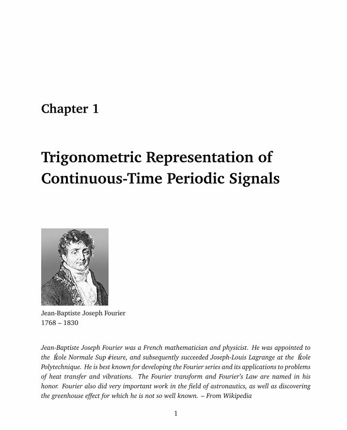
Jean-Baptiste Joseph Fourier1768 – 1830
Jean-Baptiste Joseph Fourier was a French mathematician and physicist. He was appointed tothe École Normale Supérieure, and subsequently succeeded Joseph-Louis Lagrange at the ÉcolePolytechnique. He is best known for developing the Fourier series and its applications to problemsof heat transfer and vibrations. The Fourier transform and Fourier’s Law are named in hishonor. Fourier also did very important work in the field of astronautics, as well as discoveringthe greenhouse effect for which he is not so well known. – From Wikipedia
1
CHAPTER 1. TRIGONOMETRIC REPRESENTATION OF CT PERIODIC SIGNALS
What is Fourier Analysis
When sunlight hits rain-soaked air, an interesting phenomenon happens. Water drops takethe ostensibly pure white light and split it into multiple colors. The mathematical descriptionof this process, the subject of this book, was first tackled by Isac Newton approximately400 years ago. However, even though Newton was able to show that white light is, infact, composed of other colors, he was unable to make the jump to the idea that light canbe described as waves. He called the component colors of white light “specter” or ghosts,from which we get the word spectrum. It took the development of trigonometric series andthe recognition of the fact that light can be thought of as a composite wave before Fouriercould apply these ideas to the problem of heat transfer. Although the concept of harmonictrigonometric series already existed by the time he worked on the heat transfer problem,Fourier’s contribution is considered so important that the whole field of trigonometric wave-form analysis and synthesis now bears his name, Fourier analysis.
Fourier developed the following partial differential equation called the Diffusion equation todescribe heat transfer through solids and other media. Here, v is a function representing themeasure of heat and K is the heat diffusion constant of the material.
∂ v∂ t= K
∂ 2v∂ x2
(1.1)
Fourier observed that the most general solution to this equation was given as a linear summationof sinusoids, i.e., sine and cosine waves of the form:
v(k, x) =∞∑
k=0
ak sin kx + bk cos kx
(1.2)
This led Fourier to conclude that an arbitrary wave can be represented as a sum of an infinitenumber of weighted sinusoids, i.e., sine and cosine waves. This sinusoid summation conceptis now known as the Fourier series. This book is all about this simple but important idea.
Fourier analysis is applicable to a wide variety of disciplines and not just signal processing,where it is now an essential tool. In addition, Fourier analysis is used in image processing,geothermal and seismic studies, stochastic biological processes, quantum mechanics, acous-tics, and even finance.
The Fourier analysis of waves or signals is similar to the concept of compound analysis inchemistry. Instead of atoms coming together to form a myriad of compounds, in signalprocessing sinusoids can be thought of as doing the same thing. A particular set of these
2

CHAPTER 1. TRIGONOMETRIC REPRESENTATION OF CT PERIODIC SIGNALS
sinusoids is called the basis set. Just as a compound may consist of two units of one elementand four units of another, an arbitrary wave can consist of two units of one base wave andfour units of another. Hence, we can create a particular wave by putting together some basiswaves from the set. This process is called Synthesis. Conversely, the process of decomposingan arbitrary wave into a set of basis waves is termed Analysis. These two complementaryand linear processes fall under the name of Fourier analysis and its analog, the Fouriertransform. In Fourier analysis, the basis set of waves is periodic sinusoids.
(a) Fourier Analysis (b) Fourier Synthesis
Figure 1.1: Fourier analysis is used to understand composite waves. (a) Analysis: breaking a givensignal into sine and cosine components and (b) Synthesis: adding certain sine and cosines to create a
desired signal.
Possibly, it was the solution of Eq. (1.1) that led Fourier to notice that summation of harmonicsine and cosine waves leads to some interesting looking periodic waves. From this, heposited that conversely it is also possible to create any periodic signal by the summationof a particular set of harmonic sinusoids. This may not seem like a big thing now but it wasa revolutionary insight at the time.
Fourier’s discovery was met with incredulity at first. Rightfully so, many of his contemporariesdid not accept that his idea was truly general and applied to all signals. After some years ofwork by Fourier as well as other famous mathematicians of the age, his theorem was upheld,albeit not under all conditions and not for all types of signals. Subsequent developmentled to the Fourier transform, the extension of Fourier’s original idea to nonperiodic signals.However, this computationally demanding concept languished for over 100 years, until thedevelopment of the Fast Fourier Transform (FFT), by J.W. Cooley and John Tukey in 1965.The FFT, an algorithmic technique, made the computation of Fourier series simpler andquicker and finally allowed Fourier analysis to be recognized and used widely. It is nowthe premier tool of analysis in many fields.
3
CHAPTER 1. TRIGONOMETRIC REPRESENTATION OF CT PERIODIC SIGNALS
Frequency and Time Domain Views of a Signal
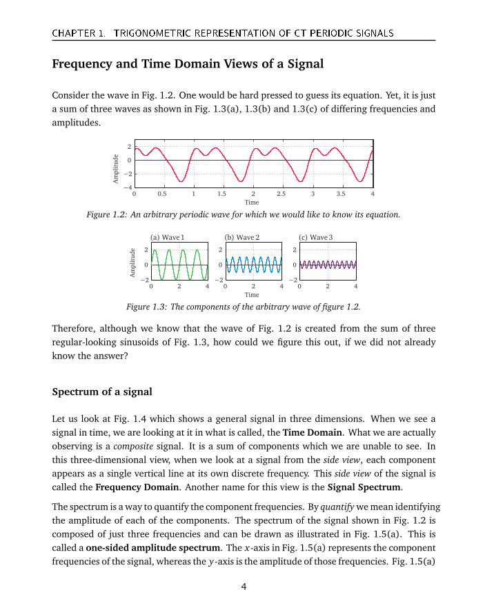
Consider the wave in Fig. 1.2. One would be hard pressed to guess its equation. Yet, it is justa sum of three waves as shown in Fig. 1.3(a), 1.3(b) and 1.3(c) of differing frequencies andamplitudes.
0 0.5 1 1.5 2 2.5 3 3.5 4−4
−2
0
2
Time
Amplitude
Figure 1.2: An arbitrary periodic wave for which we would like to know its equation.
0 2 4−2
0
2
Amplitude
(a) Wave 1
0 2 4−2
0
2
Time
(b) Wave 2
0 2 4−2
0
2
(c) Wave 3
Figure 1.3: The components of the arbitrary wave of figure 1.2.
Therefore, although we know that the wave of Fig. 1.2 is created from the sum of threeregular-looking sinusoids of Fig. 1.3, how could we figure this out, if we did not alreadyknow the answer?
Spectrum of a signal
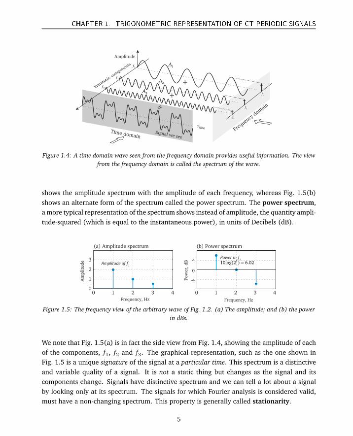
Let us look at Fig. 1.4 which shows a general signal in three dimensions. When we see asignal in time, we are looking at it in what is called, the Time Domain. What we are actuallyobserving is a composite signal. It is a sum of components which we are unable to see. Inthis three-dimensional view, when we look at a signal from the side view, each componentappears as a single vertical line at its own discrete frequency. This side view of the signal iscalled the Frequency Domain. Another name for this view is the Signal Spectrum.
The spectrum is a way to quantify the component frequencies. By quantify we mean identifyingthe amplitude of each of the components. The spectrum of the signal shown in Fig. 1.2 iscomposed of just three frequencies and can be drawn as illustrated in Fig. 1.5(a). This iscalled a one-sided amplitude spectrum. The x-axis in Fig. 1.5(a) represents the componentfrequencies of the signal, whereas the y-axis is the amplitude of those frequencies. Fig. 1.5(a)
4
CHAPTER 1. TRIGONOMETRIC REPRESENTATION OF CT PERIODIC SIGNALS
Time
3f
2f
1f
Harmonic
componen
ts
Amplitude
+
+
=
1f
2f
3f
Signal we see
Frequen
cy d
omai
n
1A
2A
3A
Time domain
Figure 1.4: A time domain wave seen from the frequency domain provides useful information. The viewfrom the frequency domain is called the spectrum of the wave.
shows the amplitude spectrum with the amplitude of each frequency, whereas Fig. 1.5(b)shows an alternate form of the spectrum called the power spectrum. The power spectrum,a more typical representation of the spectrum shows instead of amplitude, the quantity ampli-tude-squared (which is equal to the instantaneous power), in units of Decibels (dB).
0 1 2 3 40
1
2
3
Am
pli
tud
e
Frequency, Hz
0 1 2 3 4
0
-4
4
Pow
er,
dB
Frequency, Hz
(a) Amplitude spectrum (b) Power spectrum
Amplitude of f1
Power in f1
210log(2 ) 6.02=
Figure 1.5: The frequency view of the arbitrary wave of Fig. 1.2. (a) The amplitude; and (b) the powerin dBs.
We note that Fig. 1.5(a) is in fact the side view from Fig. 1.4, showing the amplitude of eachof the components, f1, f2 and f3. The graphical representation, such as the one shown inFig. 1.5 is a unique signature of the signal at a particular time. This spectrum is a distinctiveand variable quality of a signal. It is not a static thing but changes as the signal and itscomponents change. Signals have distinctive spectrum and we can tell a lot about a signalby looking only at its spectrum. The signals for which Fourier analysis is considered valid,must have a non-changing spectrum. This property is generally called stationarity.
5
CHAPTER 1. TRIGONOMETRIC REPRESENTATION OF CT PERIODIC SIGNALS
Fundamental waves and their harmonics
The basic building blocks of Fourier analysis are a set of harmonic sinusoids, called thebasis set. The basis set is our tinker-toy from which we can construct a variety of waves.The set contains an infinite number of sinusoids of differing frequencies related in a specialway known as harmonic.
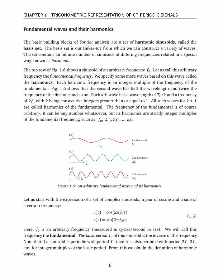
The top row of Fig. 1.6 shows a sinusoid of an arbitrary frequency, f0. Let us call this arbitraryfrequency the fundamental frequency. We specify some more waves based on this wave calledthe harmonics. Each harmonic frequency is an integer multiple of the frequency of thefundamental. Fig. 1.6 shows that the second wave has half the wavelength and twice thefrequency of the first one and so on. Each kth wave has a wavelength of T0/k and a frequencyof k f0 with k being consecutive integers greater than or equal to 1. All such waves for k > 1are called harmonics of the fundamental. The frequency of the fundamental is of coursearbitrary, it can be any number whatsoever, but its harmonics are strictly integer multiplesof the fundamental frequency, such as: f0, 2 f0, 3 f0, ... k f0.
Fundamental
2nd harmonic
3rd harmonic
0T
0
2
T
0
3
T
0f
02 f
03 f
(a)
(b)
(c)
Figure 1.6: An arbitrary fundamental wave and its harmonics.
Let us start with the expression of a set of complex sinusoids; a pair of cosine and a sine ofa certain frequency:
c(t) = cos(2π f0 t)
s(t) = sin(2π f0 t)(1.3)
Here, f0 is an arbitrary frequency (measured in cycles/second or Hz). We will call thisfrequency the fundamental. The basic period T , of this sinusoid is the inverse of the frequency.Note that if a sinusoid is periodic with period T , then it is also periodic with period 2T , 3T ,etc. for integer multiples of the basic period. From this we obtain the definition of harmonicwaves.
6
CHAPTER 1. TRIGONOMETRIC REPRESENTATION OF CT PERIODIC SIGNALS
A set of waves is harmonic if its frequency is an integer multiple of the fundamental wave’sfrequency. We can write this as a set.
c(t) = cos(2π fk t)s(t) = sin(2π fk t)
(1.4)
We have introduced an index, k in Eq. (1.4) such that each harmonic frequency is equal to ktimes the fundamental frequency, fk = k f0, with k any arbitrary integer, 0, 1, 2, . . . ,∞.
In Fourier series formulation, the index k spans all positive integers to infinity, including zero.Note that the fundamental wave or the first harmonic is often defined as the one for k = 1.Hence, the frequency of the first harmonic and the fundamental frequency are the same. Thewave obtained for k = 0 is of course nothing but a flat line. The wave for k = 2 is called thesecond harmonic and so on for higher values of the index k.
Let us rewrite the definition of the harmonics allowing the phase and the amplitude to vary.We give each harmonic a unique amplitude and phase and rewrite the harmonic signals as:
ck(t) = ak cos(2πk f0 t +φk)
sk(t) = bk sin(2πk f0 t +φk)(1.5)
The wave ck(t) is a cosine wave of kth harmonic frequency or k f0, its amplitude being ak
and the phase in radians being φk. The signal sk(t) is a sine wave with similarly uniqueamplitude and phase for the same harmonic frequency, k f0. Now although the frequenciesare still related by multiples of integer k, we are allowing the amplitude and the phase ofeach harmonic to be different. Such waves are still considered harmonic. The amplitudecoefficient ak for a cosine and bk for a sine are now arbitrary.
What is amplitude? Amplitude is often thought of as the value of a wave’s height aboveits mean value at any particular time. The amplitude can be either positive or negative,indicating where it is being measured, above or below the mean value. If a sinusoid is givenby the expression: a cos(ωt), then the instantaneous value of the sinusoid (±1) is scaled bythe coefficient, a. The peak value is never more than a, hence this coefficient is the peakamplitude. This coefficient, is called the amplitude of the wave. It is one half of the wave’sfull excursion above and below its mean. In Eq. (1.5), the terms ak and bk are the amplitudesof the waves.
What is phase? The argument of a sinusoid sin(θ ), is in fact an angle, or the term θ .However, in signal processing, we often need to represent a sinusoid as a function of time.We do this by writing the sinusoid as sin(ωt), where ω is the radial frequency defined interms of angles per time. Both forms of the sinusoid argument, the θ and its equivalent form
7
CHAPTER 1. TRIGONOMETRIC REPRESENTATION OF CT PERIODIC SIGNALS
ωt, are called the instantaneous phase of the sinusoid. We can shift a sinusoid, or in factany wave in time, by adding a term, φ, to the instantaneous phase, θ , writing the sinusoidas sin(θ +φ). This second term, φ, is assumed to be fixed as a function of time (for linearsystems) and is commonly called the phase. This can be confusing, because we have twoquantities here, both called phase. The total phase at any time is made up of these two parts,one a fixed quantity and the other changing with time. However, generally when we sayphase, we are referring not to the instantaneous quantity ωt, but to the fixed quantity, φ.This term is more properly called the phase shift but the qualifier word shift is often left off.In Eq. (1.5), the term φk is the phase (shift) for the kth wave.
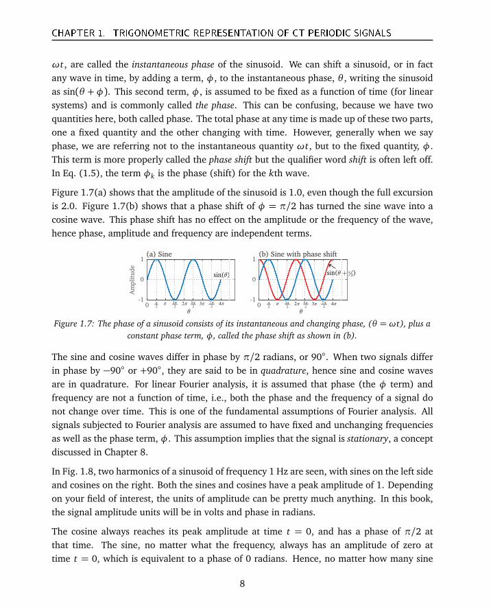
Figure 1.7(a) shows that the amplitude of the sinusoid is 1.0, even though the full excursionis 2.0. Figure 1.7(b) shows that a phase shift of φ = π/2 has turned the sine wave into acosine wave. This phase shift has no effect on the amplitude or the frequency of the wave,hence phase, amplitude and frequency are independent terms.
0-1
0
1
Am
pli
tud
e
(a) Sine
0-1
0
1(b) Sine with phase shift
π 2π2
π 3
2
π 5
2
π 3π 7
2
π 4π π 2π2
π 3
2
π 5
2
π 3π 7
2
π 4π
θθ
sin( )θ 2sin( )πθ+
Figure 1.7: The phase of a sinusoid consists of its instantaneous and changing phase, (θ =ωt), plus aconstant phase term, φ, called the phase shift as shown in (b).
The sine and cosine waves differ in phase by π/2 radians, or 90. When two signals differin phase by −90 or +90, they are said to be in quadrature, hence sine and cosine wavesare in quadrature. For linear Fourier analysis, it is assumed that phase (the φ term) andfrequency are not a function of time, i.e., both the phase and the frequency of a signal donot change over time. This is one of the fundamental assumptions of Fourier analysis. Allsignals subjected to Fourier analysis are assumed to have fixed and unchanging frequenciesas well as the phase term, φ. This assumption implies that the signal is stationary, a conceptdiscussed in Chapter 8.
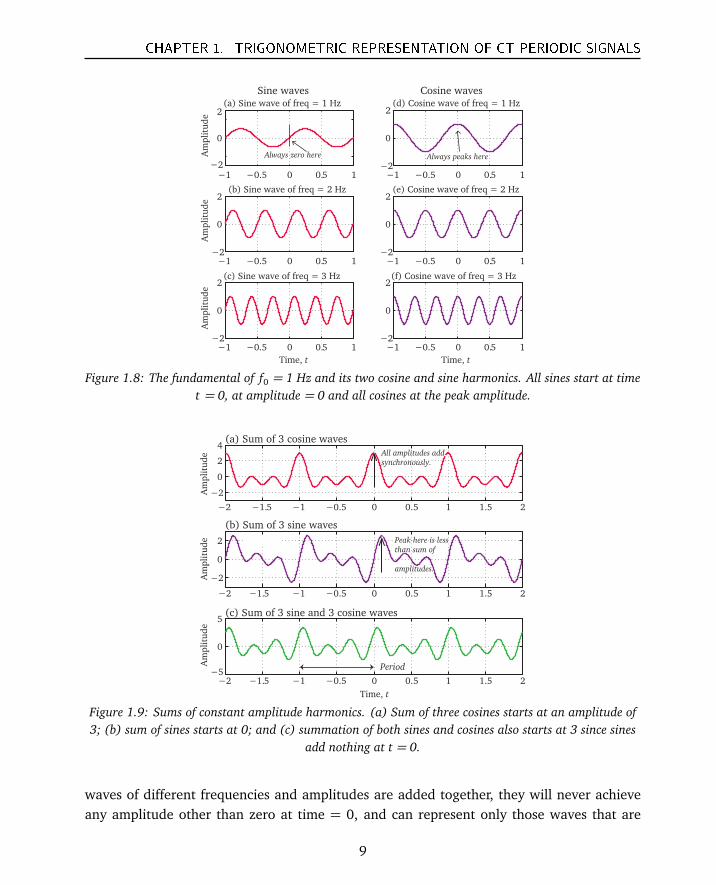
In Fig. 1.8, two harmonics of a sinusoid of frequency 1 Hz are seen, with sines on the left sideand cosines on the right. Both the sines and cosines have a peak amplitude of 1. Dependingon your field of interest, the units of amplitude can be pretty much anything. In this book,the signal amplitude units will be in volts and phase in radians.
The cosine always reaches its peak amplitude at time t = 0, and has a phase of π/2 atthat time. The sine, no matter what the frequency, always has an amplitude of zero attime t = 0, which is equivalent to a phase of 0 radians. Hence, no matter how many sine
8
CHAPTER 1. TRIGONOMETRIC REPRESENTATION OF CT PERIODIC SIGNALS
−1 −0.5 0 0.5 1−2
0
2(a) Sine wave of freq = 1 Hz
−1 −0.5 0 0.5 1−2
0
2(b) Sine wave of freq = 2 Hz
−1 −0.5 0 0.5 1−2
0
2(c) Sine wave of freq = 3 Hz
−1 −0.5 0 0.5 1−2
0
2(d) Cosine wave of freq = 1 Hz
−1 −0.5 0 0.5 1−2
0
2(e) Cosine wave of freq = 2 Hz
−1 −0.5 0 0.5 1−2
0
2(f) Cosine wave of freq = 3 Hz
Am
pli
tud
eA
mpli
tud
eA
mpli
tud
e
Sine waves Cosine waves
Time, t Time, t
Always zero here Always peaks here
Figure 1.8: The fundamental of f0 = 1 Hz and its two cosine and sine harmonics. All sines start at timet = 0, at amplitude = 0 and all cosines at the peak amplitude.
−2 −1.5 −1 −0.5 0 0.5 1 1.5 2
−2
0
2
(b) Sum of 3 sine waves
−2 −1.5 −1 −0.5 0 0.5 1 1.5 2
−2
0
2
4(a) Sum of 3 cosine waves
−2 −1.5 −1 −0.5 0 0.5 1 1.5 2−5
0
5(c) Sum of 3 sine and 3 cosine waves
Am
pli
tud
eA
mpli
tud
eA
mpli
tud
e
All amplitudes add
synchronously.
All amplitudes add
synchronously.
All amplitudes add
synchronously.
Period
Time, t
Peak here is less
than sum of
amplitudes.
Peak here is less
than sum of
amplitudes.
Peak here is less
than sum of
amplitudes.
Figure 1.9: Sums of constant amplitude harmonics. (a) Sum of three cosines starts at an amplitude of3; (b) sum of sines starts at 0; and (c) summation of both sines and cosines also starts at 3 since sines
add nothing at t = 0.
waves of different frequencies and amplitudes are added together, they will never achieveany amplitude other than zero at time = 0, and can represent only those waves that are
9
CHAPTER 1. TRIGONOMETRIC REPRESENTATION OF CT PERIODIC SIGNALS
zero-valued at time t = 0. Similarly, the addition of various cosines will not achieve anamplitude of 0 at time t = 0.
Harmonics as Basis Functions
In Fig. 1.9 three cosine and three sine waves with amplitude of 1 are added together, respectively.After the addition of these three waves, it is seen that the cosines in Fig. 1.9(a) add such thatthe peak is equal to 3. This happens because the cosine is an even wave. The cosines addconstructively at time t = 0 and at other times that are integer-periods away. The sum ofthe three sine waves added together in Fig. 1.9(b) however, looks strange. This asymmetryis a consequence of the sine wave being an odd wave. In Fig. 1.9(c), the three sine andthree cosine waves are all added together. The behavior of this summation defies an easyexplanation.
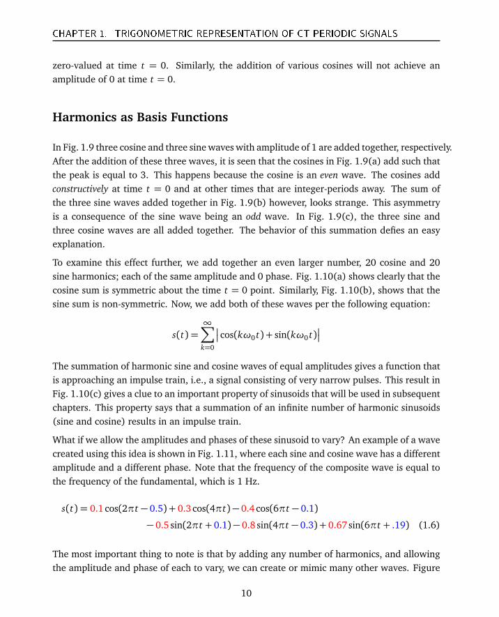
To examine this effect further, we add together an even larger number, 20 cosine and 20sine harmonics; each of the same amplitude and 0 phase. Fig. 1.10(a) shows clearly that thecosine sum is symmetric about the time t = 0 point. Similarly, Fig. 1.10(b), shows that thesine sum is non-symmetric. Now, we add both of these waves per the following equation:
s(t) =∞∑
k=0
cos(kω0 t) + sin(kω0 t)
The summation of harmonic sine and cosine waves of equal amplitudes gives a function thatis approaching an impulse train, i.e., a signal consisting of very narrow pulses. This result inFig. 1.10(c) gives a clue to an important property of sinusoids that will be used in subsequentchapters. This property says that a summation of an infinite number of harmonic sinusoids(sine and cosine) results in an impulse train.
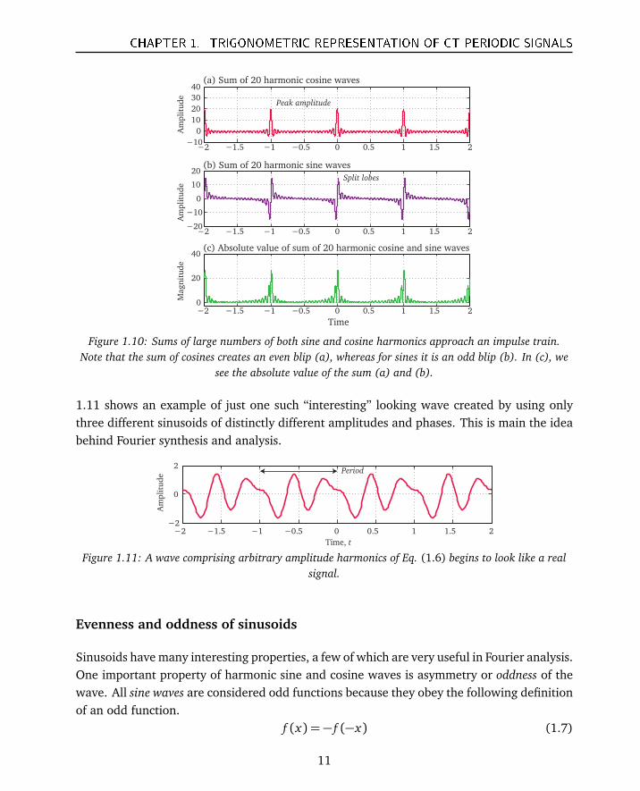
What if we allow the amplitudes and phases of these sinusoid to vary? An example of a wavecreated using this idea is shown in Fig. 1.11, where each sine and cosine wave has a differentamplitude and a different phase. Note that the frequency of the composite wave is equal tothe frequency of the fundamental, which is 1 Hz.
s(t) = 0.1 cos(2πt − 0.5) + 0.3cos(4πt)− 0.4 cos(6πt − 0.1)
− 0.5 sin(2πt + 0.1)− 0.8 sin(4πt − 0.3) + 0.67 sin(6πt + .19) (1.6)
The most important thing to note is that by adding any number of harmonics, and allowingthe amplitude and phase of each to vary, we can create or mimic many other waves. Figure
10
CHAPTER 1. TRIGONOMETRIC REPRESENTATION OF CT PERIODIC SIGNALS
−2 −1.5 −1 −0.5 0 0.5 1 1.5 2−10
0
10
20
30
40(a) Sum of 20 harmonic cosine waves
−2 −1.5 −1 −0.5 0 0.5 1 1.5 2−20
−10
0
10
20(b) Sum of 20 harmonic sine waves
−2 −1.5 −1 −0.5 0 0.5 1 1.5 20
20
40(c) Absolute value of sum of 20 harmonic cosine and sine waves
Am
pli
tud
eA
mpli
tud
eM
agn
itu
de
Time
Peak amplitude
Split lobes
Figure 1.10: Sums of large numbers of both sine and cosine harmonics approach an impulse train.Note that the sum of cosines creates an even blip (a), whereas for sines it is an odd blip (b). In (c), we
see the absolute value of the sum (a) and (b).
1.11 shows an example of just one such “interesting” looking wave created by using onlythree different sinusoids of distinctly different amplitudes and phases. This is main the ideabehind Fourier synthesis and analysis.
−2 −1.5 −1 −0.5 0 0.5 1 1.5 2−2
0
2
Am
pli
tud
e
Time, t
Period
Figure 1.11: A wave comprising arbitrary amplitude harmonics of Eq. (1.6) begins to look like a realsignal.
Evenness and oddness of sinusoids
Sinusoids have many interesting properties, a few of which are very useful in Fourier analysis.One important property of harmonic sine and cosine waves is asymmetry or oddness of thewave. All sine waves are considered odd functions because they obey the following definitionof an odd function.
f (x) = − f (−x) (1.7)
11
CHAPTER 1. TRIGONOMETRIC REPRESENTATION OF CT PERIODIC SIGNALS
If you look at a sine wave, you see that it starts with an amplitude of 0 at time t = 0. Ifwe were to flip it about the y-axis, the images would not overlap. However, if one of thesides was first flipped about the x-axis, then they do overlap. This describes the oddness ofsignals. It requires two flips for values to coincide, as we can see from the two negative signsin Eq. (1.7).
The cosine waves on the other hand are called even functions by a similar definition. Thetwo sides of a cosine wave, if flipped about the y-axis, would overlap, hence there is onlyone negative in the equation below for even symmetry.
f (x) = f (−x) (1.8)
By the superposition principle, if multiple odd waves are summed together, the resultingwave will remain odd. In contrast, if multiple even waves are summed, then the resultingwave will remain even, and a mixture will have no symmetry. This becomes important whensynthesizing, which is the process of putting some waves together to make a desired wave.If a wave to be synthesized is purely an odd, or an even function, then it will only containsines, or cosines, respectively, depending on its symmetry.
Making waves
Using the idea of harmonic summation, we can create a variety of waveforms. All we needto do is to change the amplitudes and the phases of the harmonics as we see fit. Certaincombinations of these parameters lead to great-looking and useful waves that are periodicwith the frequency of the fundamental.
Square waves
Now we examine the construction of a square wave. A square wave is not actually square inany particular sense. It is a wave where each period looks somewhat like two rectangles ofopposite signs, as seen in Fig. 1.12(d). Yes, it has wiggles in it, and, it is not actually square.The square waves are very useful in signal processing and are used for data transmission. Itis amazing that we can create them by just adding a bunch of sinusoids. The more sinusoidswe add to the summation, the better the wave looks, with the wiggles getting smaller.
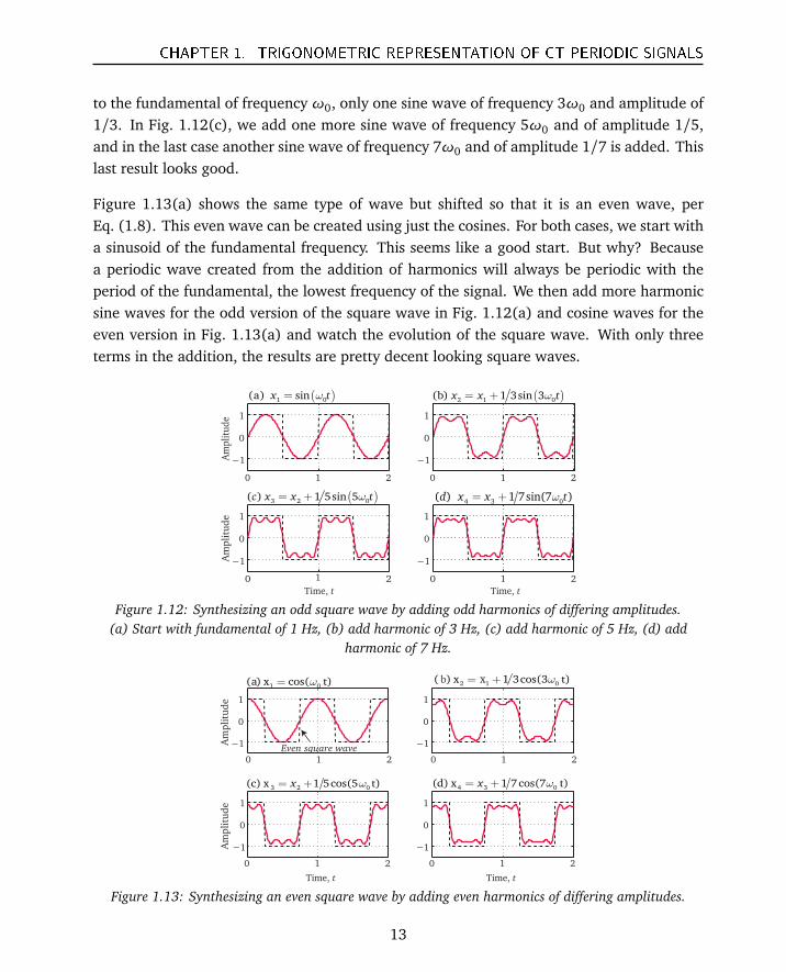
In Fig. 1.12, we have created a square wave by adding together only a few harmonic sinusoids.As the square wave shown in Fig. 1.12(a) is an odd function, we know that only sine wavesare needed in its construction, a process also called synthesis. In Fig. 1.12(b), we have added
12
CHAPTER 1. TRIGONOMETRIC REPRESENTATION OF CT PERIODIC SIGNALS
to the fundamental of frequency ω0, only one sine wave of frequency 3ω0 and amplitude of1/3. In Fig. 1.12(c), we add one more sine wave of frequency 5ω0 and of amplitude 1/5,and in the last case another sine wave of frequency 7ω0 and of amplitude 1/7 is added. Thislast result looks good.
Figure 1.13(a) shows the same type of wave but shifted so that it is an even wave, perEq. (1.8). This even wave can be created using just the cosines. For both cases, we start witha sinusoid of the fundamental frequency. This seems like a good start. But why? Becausea periodic wave created from the addition of harmonics will always be periodic with theperiod of the fundamental, the lowest frequency of the signal. We then add more harmonicsine waves for the odd version of the square wave in Fig. 1.12(a) and cosine waves for theeven version in Fig. 1.13(a) and watch the evolution of the square wave. With only threeterms in the addition, the results are pretty decent looking square waves.
0 1 2
−1
0
1
0 1 2
−1
0
1
0 1 2
−1
0
1
0 1 2
−1
0
1
( )2 1 0( ) 1 3sin 3b x x tω= +( )1 0( ) sina x tω=
( )3 2 0( ) 1 5sin 5c x x tω= +
Amplitude
Time, t
Amplitude
Time, t
4 3 0( ) 1 7sin(7 )d x x tω= +
Figure 1.12: Synthesizing an odd square wave by adding odd harmonics of differing amplitudes.(a) Start with fundamental of 1 Hz, (b) add harmonic of 3 Hz, (c) add harmonic of 5 Hz, (d) add
harmonic of 7 Hz.
0 1 2
−1
0
1
0 1 2
−1
0
1
0 1 2
−1
0
1
0 1 2
−1
0
1
1 0( ) x cos( t)a ω= 2 1 0( ) x 1 3cos(3 t)ω= +
3 2 0(c) x 1 5cos(5 t)x ω= + 4 3 0(d) x 1 7cos(7 t)x ω= +
Even square wave
Amplitude
Amplitude
Time, t Time, t
b x
Figure 1.13: Synthesizing an even square wave by adding even harmonics of differing amplitudes.
13
CHAPTER 1. TRIGONOMETRIC REPRESENTATION OF CT PERIODIC SIGNALS
Each addition of a sine wave (or a cosine) with a specific frequency and amplitude makesthe synthesized wave appear closer to a square wave. We are, in fact, cooking up interestingrecipes for making all kinds of waves using specific “quantities” of sinusoids. The quantitieswe vary are the amplitude and the phase of each harmonic. Collectively, the amplitude andthe phase of a particular harmonic is called its coefficient. So to create a particular wave,we are controlling or changing the coefficients of the harmonics.
Here are the recipes for the two types of square waves, the odd and the even. The ingredientlist is limited, as we used only three terms beyond the fundamental, which is underlined.
x1 = sin(ω0 t) +13
sin(3ω0 t) +15
sin(5ω0 t) +17
sin(7ω0 t)
x2 = cos(ω0 t)−13
cos(3ω0 t) +15
cos(5ω0 t)−17
cos(7ω0 t)(1.9)
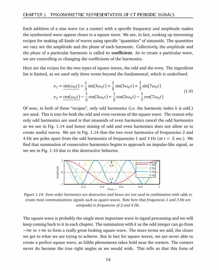
Of note, in both of these “recipes”, only odd harmonics (i.e. the harmonic index k is odd.)are used. This is true for both the odd and even versions of the square wave. The reason whyonly odd harmonics are used is that sinusoids of even harmonics cancel the odd harmonicsas we see in Fig. 1.14 and hence mixing of odd and even harmonics does not allow us tocreate useful waves. We see in Fig. 1.14 that the two even harmonics of frequencies 2 and4 Hz are poles apart from the odd harmonics of frequencies 1 and 3 Hz (at t = .5 sec.). Wefind that summation of consecutive harmonics begins to approach an impulse-like signal, aswe see in Fig. 1.10 due to this destructive behavior.
0.2 0.4 0.6 0.8 1−1
0
1
1,3
2,41
2
3
4
Amplitude
Time, t
1 Hz
2 Hz
3 Hz
4 Hz
Figure 1.14: Even order harmonics are destructive and hence are not used in combination with odds tocreate most communications signals such as square waves. Note here that frequencies 1 and 3 Hz are
antipodal to frequencies of 2 and 4 Hz.
The square wave is probably the single most important wave in signal processing and we willkeep coming back to it in each chapter. The summation with k as the odd integer can go from−∞ to +∞ to form a really great looking square wave. The more terms we add, the closerwe get to what we are trying to achieve. But in fact for square waves, we are never able tocreate a perfect square wave, as Gibbs phenomena takes hold near the corners. The cornersnever do become the true right angles as we would wish. This tells us that this form of
14
CHAPTER 1. TRIGONOMETRIC REPRESENTATION OF CT PERIODIC SIGNALS
harmonic representation, despite our best efforts, may not result in a perfect reconstructionfor every signal, for example square waves.
Gibbs phenomenon
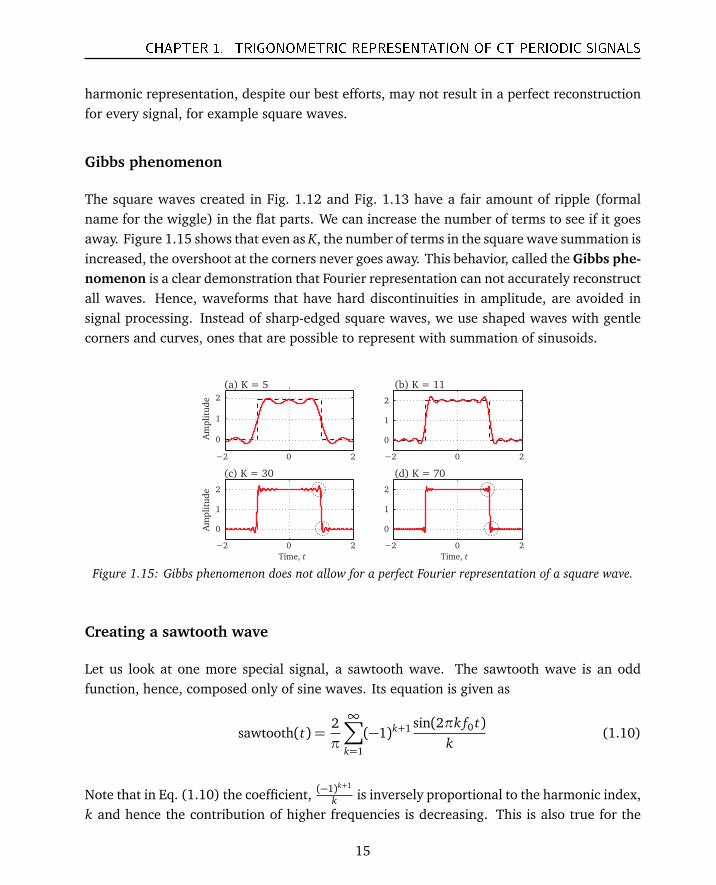
The square waves created in Fig. 1.12 and Fig. 1.13 have a fair amount of ripple (formalname for the wiggle) in the flat parts. We can increase the number of terms to see if it goesaway. Figure 1.15 shows that even as K, the number of terms in the square wave summation isincreased, the overshoot at the corners never goes away. This behavior, called the Gibbs phe-nomenon is a clear demonstration that Fourier representation can not accurately reconstructall waves. Hence, waveforms that have hard discontinuities in amplitude, are avoided insignal processing. Instead of sharp-edged square waves, we use shaped waves with gentlecorners and curves, ones that are possible to represent with summation of sinusoids.
−2 0 2
0
1
2
−2 0 2
0
1
2
−2 0 2
0
1
2
−2 0 2
0
1
2
Am
pli
tud
eA
mpli
tud
e
(a) K = 5 (b) K = 11
(c) K = 30 (d) K = 70
Time, t Time, t
Figure 1.15: Gibbs phenomenon does not allow for a perfect Fourier representation of a square wave.
Creating a sawtooth wave
Let us look at one more special signal, a sawtooth wave. The sawtooth wave is an oddfunction, hence, composed only of sine waves. Its equation is given as
sawtooth(t) =2π
∞∑
k=1
(−1)k+1 sin(2πk f0 t)k
(1.10)
Note that in Eq. (1.10) the coefficient, (−1)k+1
k is inversely proportional to the harmonic index,k and hence the contribution of higher frequencies is decreasing. This is also true for the
15
CHAPTER 1. TRIGONOMETRIC REPRESENTATION OF CT PERIODIC SIGNALS
0 1 2 3−0.5
0
0.5
0 1 2 3−0.5
0
0.5
0 1 2 3−0.5
0
0.5
0 1 2 3−0.5
0
0.5
(a) K = 1 (b) K = 5
(c) K = 11 (d) K = 20Amplitude
Amplitude
Time, t Time, t
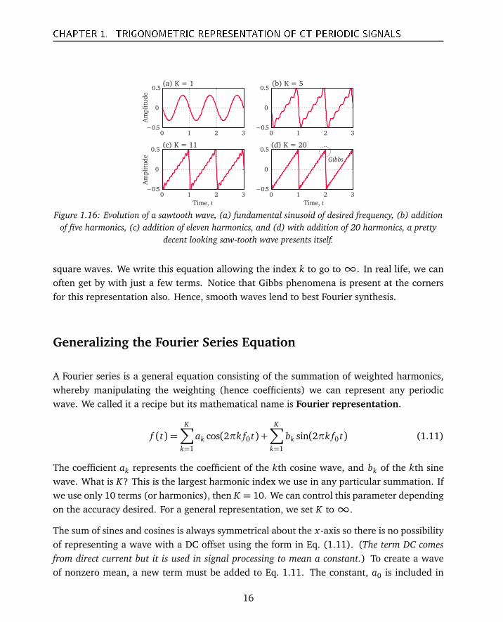
Gibbs
Figure 1.16: Evolution of a sawtooth wave, (a) fundamental sinusoid of desired frequency, (b) additionof five harmonics, (c) addition of eleven harmonics, and (d) with addition of 20 harmonics, a pretty
decent looking saw-tooth wave presents itself.
square waves. We write this equation allowing the index k to go to∞. In real life, we canoften get by with just a few terms. Notice that Gibbs phenomena is present at the cornersfor this representation also. Hence, smooth waves lend to best Fourier synthesis.
Generalizing the Fourier Series Equation
A Fourier series is a general equation consisting of the summation of weighted harmonics,whereby manipulating the weighting (hence coefficients) we can represent any periodicwave. We called it a recipe but its mathematical name is Fourier representation.
f (t) =K∑
k=1
ak cos(2πk f0 t) +K∑
k=1
bk sin(2πk f0 t) (1.11)
The coefficient ak represents the coefficient of the kth cosine wave, and bk of the kth sinewave. What is K? This is the largest harmonic index we use in any particular summation. Ifwe use only 10 terms (or harmonics), then K = 10. We can control this parameter dependingon the accuracy desired. For a general representation, we set K to∞.
The sum of sines and cosines is always symmetrical about the x-axis so there is no possibilityof representing a wave with a DC offset using the form in Eq. (1.11). (The term DC comesfrom direct current but it is used in signal processing to mean a constant.) To create a waveof nonzero mean, a new term must be added to Eq. 1.11. The constant, a0 is included in
16
CHAPTER 1. TRIGONOMETRIC REPRESENTATION OF CT PERIODIC SIGNALS
Eq. (1.12) so we can create waves that can move up (or down) from the x-axis.
f (t) = a0 +∞∑
k=1
ak cos(2π fk t) +∞∑
k=1
bk sin(2π fk t) (1.12)
Eq. (1.12) is called the Fourier series equation. The coefficients a0, ak, bk are called theFourier Series Coefficients (FSC). The process of Fourier analysis consists of computingthese three types of coefficients, given an arbitrary periodic wave, f (t).
Multiple ways of writing the Fourier series equation
There are several different forms of the Fourier series equation in literature, and that canmake understanding this equation harder.
The following representation uses the radial frequency, ωk = 2π fk to make the equationsimpler to type. We can write this form of Fourier series as:
f (t) = a0 +∞∑
k=1
ak cos(ωk t) +∞∑
k=1
bk sin(ωk t) (1.13)
Now, we define T0 as the period of the fundamental frequency.
T0 =1f0
Then the period of the kth harmonic becomes T0/k and its frequency, fk = k/T0. Wecan alternately write the Fourier series equation by adopting this form of the frequency inEq. (1.14).
f (t) = a0 +∞∑
k=1
ak cos
2πkT0
t
+∞∑
k=1
bk sin
2πkT0
t
(1.14)
We can shorten the Fourier series equation by starting at zero frequency, hence index kstarts at 0 instead of 1. Now the DC term disappears as it is included as the zero frequencycoefficient obtained by setting the index k = 0. Here is this form with the DC term gone:
f (t) =∞∑
k=0
ak cos(2π fk t) + bk sin(2π fk t) (1.15)
17
CHAPTER 1. TRIGONOMETRIC REPRESENTATION OF CT PERIODIC SIGNALS
This can be simplified further by getting rid of the sine term altogether. Sines and cosinesare really the same thing, one is just the shifted version of the other. The representation inEq. (1.13) can be written solely with cosines with a shift. This way sine becomes a cosinewith a π/2 shift and we get this form of the equation.
f (t) = a0 +∞∑
k=1
ck cos(ωk t +φk) (1.16)
In this form, each harmonic, whether a sine or a cosine, can be thought of as a cosine ofsome phase. Hence each harmonic is represented by two cosines, one with a zero phase shiftand the other with a shift of π/2. Now the whole expression uses only cosine wave and theindex, k spans not from 0 to 1, but from −∞ to +∞.
f (t) = c1 cos(ω1 t ±φ1) + c2 cos(ω2 t ±φ2) + c3 cos(ω3 t ±φ3) + . . .
Fourier series in complex exponential form
In its most important representation, the complex representation, the Fourier series is writtenas:
f (t) =∞∑
k=−∞Cke j2π k
T0t (1.17)
Here, we introduce a new term, the complex exponential, as underlined in Eq. (1.17). Thecomplex exponential (CE) represents both a sine and a cosine in one concise form. In thenext chapter, we will discuss this function in detail. The expanded form of the Fourier seriesin terms of the complex exponential looks like this:
f (t) = C0 + C1e j2π 1T0
t + C2e j2π 2T0
t + C3e j2π 3T0
t + . . .
This form shows that we can create a periodic function by summing together complex expo-nentials. Although the complex form of the Fourier series is scary looking, it is the mostcommonly used form. In the next chapter, we will look at how it is derived and why we useit in Fourier analysis. All these different representations of the Fourier series are identicaland mean exactly the same thing. They are all different ways in which you see the Fourierseries equation written in books.
18

CHAPTER 1. TRIGONOMETRIC REPRESENTATION OF CT PERIODIC SIGNALS
The Fourier Analysis
The process of adding together a bunch of sinusoids to create useful waves is called the Syn-thesis process. Synthesis of waveforms, is of course, interesting but what is really useful is thereverse process, that is, to take an arbitrary periodic signal and figure out its components.It’s like trying to figure out the ingredients of a particular dish. By ingredients, we meanfrequencies in the signal that contain significant power or amplitudes. This is the main use ofFourier analysis. It is called, not surprisingly, the Analysis part. What this involves is to makea guess of the fundamental frequency, f0, and then computing the amplitudes (coefficients)of a certain number of harmonics. There is no guarantee that the fundamental chosen willresult in finding all the main signal components exactly. Nevertheless, in most cases, we havea pretty good idea of signal components a-priori. So the process works well enough.
The usefulness of the process can be seen in the equation of the sawtooth wave in Eq. (1.10).The Fourier series allows us to create an estimate of the wave using a few or many terms.Hence, Fourier series represents an estimate of the true representation, the accuracy of whichdepends on the number of terms used.
The Fourier analysis process consists of finding the series coefficients. When we talk aboutFourier series coefficients (FSC), we are talking about the amplitudes of the sine and cosineharmonics, and nothing else. Once we decide on a fundamental frequency -a starting pointfor the analysis- we already know all the harmonic frequencies since they are integer multiplesof the fundamental frequency. All we have to do now is to compute the coefficients. Thefollowing are the three types of coefficients we need to compute.
1. The DC offset or the coefficient of the 0th frequency, k = 0.2. Coefficients of the cosine ak cos(2πk f0 t) with k = 1, 2,3, . . . ,∞.3. Coefficients of the sine bk sin(2πk f0 t) with k = 1,2, 3, . . . ,∞.
We will discuss each of these three types of coefficients separately and see how to computethem.
Computing a0, the DC coefficient
We are given an arbitrary periodic signal, f (t), of period T. The Fourier series says that thesignal f (t) is equivalent to a summation of K sinusoidal harmonics. Our task is to find thecoefficients of each of these harmonics starting with k = 0 to k = K . This task is calledFourier analysis.
f (t) = a0 +∞∑
k=1
ak cos(2π fk t) + bk sin(2π fk t) (1.18)
19
CHAPTER 1. TRIGONOMETRIC REPRESENTATION OF CT PERIODIC SIGNALS
The constant a0 in the Fourier series equation represents the DC offset. If our target wavehas a nonzero DC component (if its average amplitude value is not zero), then we know thata0 6= 0. But before we compute it, let’s take a look at a useful property of sine and cosinewaves. Both sine and cosine waves are symmetrical about the x-axis. When you integrate
0 0.25 0.5 0.75 1−1
0
1
Amplitude
0 0.25 0.5 0.75 1−1
0
1
Amplitude
(a) One period of sine (b) One period of cosine
Time, t Time, t
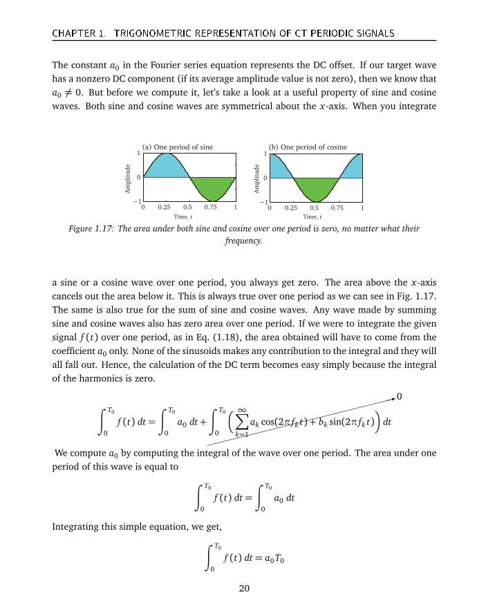
Figure 1.17: The area under both sine and cosine over one period is zero, no matter what theirfrequency.
a sine or a cosine wave over one period, you always get zero. The area above the x-axiscancels out the area below it. This is always true over one period as we can see in Fig. 1.17.The same is also true for the sum of sine and cosine waves. Any wave made by summingsine and cosine waves also has zero area over one period. If we were to integrate the givensignal f (t) over one period, as in Eq. (1.18), the area obtained will have to come from thecoefficient a0 only. None of the sinusoids makes any contribution to the integral and they willall fall out. Hence, the calculation of the DC term becomes easy simply because the integralof the harmonics is zero.
∫ T0
0
f (t) dt=
∫ T0
0
a0 dt+
:0
∫ T0
0
∞∑
k=1
ak cos(2π fk t) + bk sin(2π fk t)
dt
We compute a0 by computing the integral of the wave over one period. The area under oneperiod of this wave is equal to
∫ T0
0
f (t) dt=
∫ T0
0
a0 dt
Integrating this simple equation, we get,
∫ T0
0
f (t) dt= a0T0
20
CHAPTER 1. TRIGONOMETRIC REPRESENTATION OF CT PERIODIC SIGNALS
0 0.5 1 1.5 2
0
1
Am
pli
tud
e
(a) One period of the signal
0 0.5 1 1.5 2−2
0
2
4
Am
pli
tud
e(b) Result of integration
Time, t
Time, t
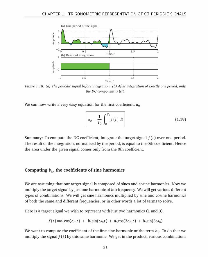
Figure 1.18: (a) The periodic signal before integration. (b) After integration of exactly one period, onlythe DC component is left.
We can now write a very easy equation for the first coefficient, a0
a0 =1T0
∫ T0
0
f (t) dt (1.19)
Summary: To compute the DC coefficient, integrate the target signal f (t) over one period.The result of the integration, normalized by the period, is equal to the 0th coefficient. Hencethe area under the given signal comes only from the 0th coefficient.
Computing bk, the coefficients of sine harmonics
We are assuming that our target signal is composed of sines and cosine harmonics. Now wemultiply the target signal by just one harmonic of kth frequency. We will get various differenttypes of combinations. We will get sine harmonics multiplied by sine and cosine harmonicsof both the same and different frequencies, or in other words a lot of terms to solve.
Here is a target signal we wish to represent with just two harmonics (1 and 3).
f (t) =a1cos(ω0 t) + b1sin(ω0 t) + a3cos(3ω0 t) + b3sin(3ω0)
We want to compute the coefficient of the first sine harmonic or the term b1. To do that wemultiply the signal f (t) by this same harmonic. We get in the product, various combinations
21
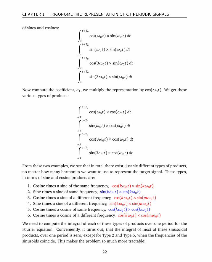
CHAPTER 1. TRIGONOMETRIC REPRESENTATION OF CT PERIODIC SIGNALS
of sines and cosines:∫ t+T0
tcos(ω0 t)× sin(ω0 t) dt
∫ t+T0
tsin(ω0 t)× sin(ω0 t) dt
∫ t+T0
tcos(3ω0 t)× sin(ω0 t) dt
∫ t+T0
tsin(3ω0 t)× sin(ω0 t) dt
Now compute the coefficient, a1, we multiply the representation by cos(ω0 t). We get thesevarious types of products:
∫ t+T0
tcos(ω0 t)× cos(ω0 t) dt
∫ t+T0
tsin(ω0 t)× cos(ω0 t) dt
∫ t+T0
tcos(3ω0 t)× cos(ω0 t) dt
∫ t+T0
tsin(3ω0 t)× cos(ω0 t) dt
From these two examples, we see that in total there exist, just six different types of products,no matter how many harmonics we want to use to represent the target signal. These types,in terms of sine and cosine products are:
1. Cosine times a sine of the same frequency, cos(kω0 t)× sin(kω0 t)2. Sine times a sine of same frequency, sin(kω0 t)× sin(kω0 t)3. Cosine times a sine of a different frequency, cos(kω0 t)× sin(mω0 t)4. Sine times a sine of a different frequency, sin(kω0 t)× sin(mω0 t)5. Cosine times a cosine of same frequency, cos(kω0 t)× cos(kω0 t)6. Cosine times a cosine of a different frequency, cos(kω0 t)× cos(mω0 t)
We need to compute the integral of each of these types of products over one period for theFourier equation. Conveniently, it turns out, that the integral of most of these sinusoidalproducts, over one period is zero, except for Type 2 and Type 5, when the frequencies of thesinusoids coincide. This makes the problem so much more tractable!
22
CHAPTER 1. TRIGONOMETRIC REPRESENTATION OF CT PERIODIC SIGNALS
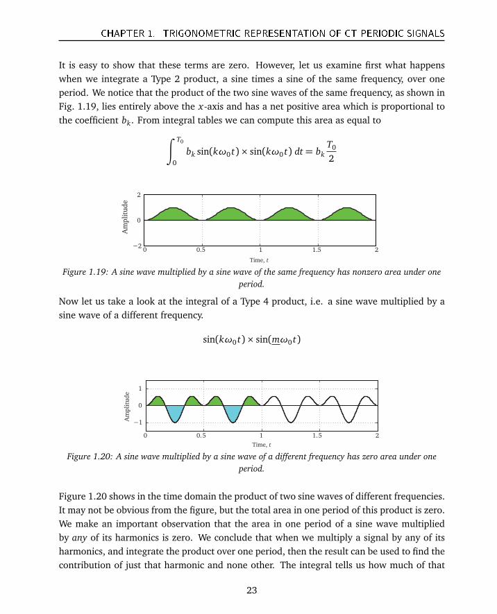
It is easy to show that these terms are zero. However, let us examine first what happenswhen we integrate a Type 2 product, a sine times a sine of the same frequency, over oneperiod. We notice that the product of the two sine waves of the same frequency, as shown inFig. 1.19, lies entirely above the x-axis and has a net positive area which is proportional tothe coefficient bk. From integral tables we can compute this area as equal to
∫ T0
0
bk sin(kω0 t)× sin(kω0 t) dt= bkT0
2
0 0.5 1 1.5 2−2
0
2
Amplitude
Time, t
Figure 1.19: A sine wave multiplied by a sine wave of the same frequency has nonzero area under oneperiod.
Now let us take a look at the integral of a Type 4 product, i.e. a sine wave multiplied by asine wave of a different frequency.
sin(kω0 t)× sin(mω0 t)
0 0.5 1 1.5 2
−1
0
1
Amplitude
Time, t
Figure 1.20: A sine wave multiplied by a sine wave of a different frequency has zero area under oneperiod.
Figure 1.20 shows in the time domain the product of two sine waves of different frequencies.It may not be obvious from the figure, but the total area in one period of this product is zero.We make an important observation that the area in one period of a sine wave multipliedby any of its harmonics is zero. We conclude that when we multiply a signal by any of itsharmonics, and integrate the product over one period, then the result can be used to find thecontribution of just that harmonic and none other. The integral tells us how much of that
23

CHAPTER 1. TRIGONOMETRIC REPRESENTATION OF CT PERIODIC SIGNALS
frequency is present in the target signal. All other sinusoids in the signal contribute nothing.The individual contribution to the signal f (t) by the kth harmonic can be written as:
∫ T0
0
bk sin(kω0 t)× sin(mω0 t) dt= 0 for k 6= m.
∫ T0
0
bk sin(kω0 t)× sin(mω0 t) dt=T0
2bk for k = m.
The same is true for cosine waves or Types 5 and 6.
∫ T0
0
ak cos(kω0 t)× cos(mω0 t) dt= 0 for k 6= m.
∫ T0
0
ak cos(kω0 t)× cos(mω0 t) dt=T0
2ak for k = m.
We see that the result of the integration of the product of two harmonics when their frequen-cies are unequal is zero. It is nonzero only when the waves have the same frequency. Hence,if we multiply our signal by its K harmonics, and integrate K times, the result for each caseis the coefficient of the harmonic being used for multiplication.
Let us now look at the product of a sine wave and a cosine wave of the same frequency, orType 1. For this case, as shown in Fig. 1.21, the net area under the product is also zero.
0 0.5 1 1.5 2
−1
0
1
Amplitude
Time, t
Figure 1.21: A sine wave multiplied by a cosine has total area of zero under one period.
The integral of Type 3 products is also zero. Hence, we note this important result; the areaunder the product of a sine and a cosine over one period is zero whether the frequencies are thesame or not. Sines and cosines just don’t agree. This is also the concept of orthogonality. Wesay that these waves are orthogonal to each other as they contribute nothing to the integral.Summarizing the results:
∫ T
0
bk cos(kω0 t)× sin(mω0 t) dt= 0 (1.20)
24
CHAPTER 1. TRIGONOMETRIC REPRESENTATION OF CT PERIODIC SIGNALS
A practical interpretation of these properties is that sine and cosine waves act as filteringsignals. When a signal, is multiplied by a sinusoid of a particular frequency, the integral isproportional to the content of that multiplying sinusoid, (by which we mean its amplitude).Hence, sinusoids behave as narrow-band filters. This is the fundamental concept of a filter.
Here are the key results we will be using in calculating the coefficients of the Fourier equation:
1. If you multiply a sine or a cosine wave by any of its harmonics, the area under theproduct is zero.
2. If you multiply a sine or a cosine of a particular frequency by itself, the area under theproduct is proportional to the Fourier coefficient of that frequency.
3. The area under a sine wave multiplied by a harmonic cosine is always zero. (Becausesine and cosine are orthogonal!)
We use these observations to compute the bk coefficients. We successively multiply the targetsignal, f (t) by a sine wave of a specific harmonic frequency and then integrate over oneperiod as in the equation below. All terms are zero except one. This term is given by:
∫ T0
0
bk sin(kω0 t) sin(kω0 t) dt=bkT0
2
From this we obtain the coefficient of the sine, bk as follows
bk =2T0
∫ T0
0
f (t) sin(kω0 t) dt (1.21)
The coefficient bk is computed by taking the target signal over one period, successivelymultiplying it with a sine wave of kth harmonic frequency and then integrating. The resultof the integration is then multiplied (or normalized) by 2/T0 to obtain the coefficient for thatparticular harmonic. If we do this K times, we get K independent bk coefficients.
Computing ak, the coefficients of cosine harmonics
Now we need to do nearly the same thing for cosine coefficients. The process of computingthe coefficients of the cosine harmonics is exactly the same as the one used for the sine waves.Instead of multiplying the target signal, f (t) by a sine wave, we multiply the target signalsequentially by a cosine wave of frequency, kω0. We get exactly the same result as when wecompute the sine coefficients. Only one term will remain in the big long multiplication for
25
CHAPTER 1. TRIGONOMETRIC REPRESENTATION OF CT PERIODIC SIGNALS
each value of k. That term is∫ T0
0
ak cos(kω0 t) cos(kω0 t) dt=akT0
2
The coefficient ak hence can be calculated by multiplying f (t) by the kth harmonic andintegrating the expression. The result is proportional to the coefficient. This expression isnearly identical to Eq. (1.21) for the bk coefficients.
ak =2T0
∫ T0
0
f (t) cos(kω0 t) dt (1.22)
In all, we do this 2K times, with K computations each for the sine and, K for the cosine.
Conceptually, the process of computing the coefficients consists of filtering the target signal,one frequency at a time. Hence, a spectrum can be seen as tiny little filter fingers that pullout the quantity (amplitude) of that harmonic in the signal.
In some simple cases, when given a signal that is composed of sinusoids, we do not need todo any calculations, as the coefficients are there in plain sight for us to see as in the followingexample.
Example 1.1. What are the FSC of this signal:
f (t) = 0.8 sin(6πt)− 0.3 cos(6πt) + .75cos(12πt)
The signal is already in the form of a Fourier series. Just by looking we can tell that thecoefficient a0 is 0. We set the fundamental frequency at 1 Hz, because then both frequenciesin the signal, 3 Hz and 6 Hz fall on a harmonic. The coefficients by observation are: a0 = 0,a3 = −0.3, b3 = 0.8 and a6 = 0.75. Of course we could have set the fundamental as 3 Hz, inwhich case the coefficients would be given as: a0 = 0, a1 = −0.3, b1 = 0.8 and a2 = 0.75.Nothing has changed except the index.
We just did our first Fourier analysis without lifting a pencil! Now something a little morecomplicated.
Example 1.2. What are the FSC of this signal:
f (t) = cos3(2πt)
26
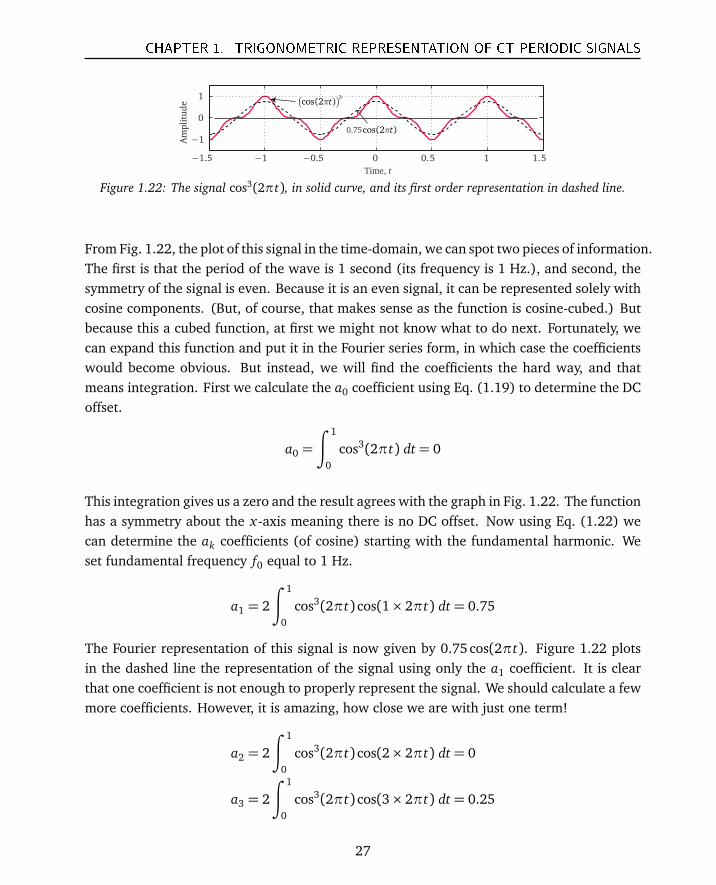
CHAPTER 1. TRIGONOMETRIC REPRESENTATION OF CT PERIODIC SIGNALS
−1.5 −1 −0.5 0 0.5 1 1.5
−1
0
1
Am
pli
tud
e ( )3
cos(2 )tπ
cos(2 )tπ0.75
Time, t
Figure 1.22: The signal cos3(2πt), in solid curve, and its first order representation in dashed line.
From Fig. 1.22, the plot of this signal in the time-domain, we can spot two pieces of information.The first is that the period of the wave is 1 second (its frequency is 1 Hz.), and second, thesymmetry of the signal is even. Because it is an even signal, it can be represented solely withcosine components. (But, of course, that makes sense as the function is cosine-cubed.) Butbecause this a cubed function, at first we might not know what to do next. Fortunately, wecan expand this function and put it in the Fourier series form, in which case the coefficientswould become obvious. But instead, we will find the coefficients the hard way, and thatmeans integration. First we calculate the a0 coefficient using Eq. (1.19) to determine the DCoffset.
a0 =
∫ 1
0
cos3(2πt) dt= 0
This integration gives us a zero and the result agrees with the graph in Fig. 1.22. The functionhas a symmetry about the x-axis meaning there is no DC offset. Now using Eq. (1.22) wecan determine the ak coefficients (of cosine) starting with the fundamental harmonic. Weset fundamental frequency f0 equal to 1 Hz.
a1 = 2
∫ 1
0
cos3(2πt) cos(1× 2πt) dt= 0.75
The Fourier representation of this signal is now given by 0.75cos(2πt). Figure 1.22 plotsin the dashed line the representation of the signal using only the a1 coefficient. It is clearthat one coefficient is not enough to properly represent the signal. We should calculate a fewmore coefficients. However, it is amazing, how close we are with just one term!
a2 = 2
∫ 1
0
cos3(2πt) cos(2× 2πt) dt= 0
a3 = 2
∫ 1
0
cos3(2πt) cos(3× 2πt) dt= 0.25
27

CHAPTER 1. TRIGONOMETRIC REPRESENTATION OF CT PERIODIC SIGNALS
With a0 = 0, a1 = 0.75, a2 = 0, and a3 = 0.25, the representation is given as:
f (t) = 0.75cos(2πt) + 0.25 cos(6πt)
This is the Fourier series representation of the signal given to us as cos3(2πt). If we continueto calculate more coefficients (for k> 3), we will see that they are all zero after a3. From this,we can say that function cosine cubed is, in fact, made up of only two cosines of frequency 1and 3 Hz. In this case, Fourier series representation is an exact representation of the signal,but this is not always the case.
Example 1.3. What are the FSC of this signal?
f (t) = sin2(2πt) + sin(2πt)
−1 −0.5 0 0.5 1 1.5
0
1
2
Am
pli
tud
e
Time, t
Figure 1.23: The signal, f (t) = sin2(2πt) + sin(2πt).
The analysis of this signal uses the ideas from the first two examples. The signal has alinear part, sin(2πt), and a non-linear part, sin2(2πt). The best way to compute its Fourierseries representation is to convert the non-linear term to a linear term. Using trigonometricidentities, we do this conversion and rewrite the signal with all linear terms as:
f (t) =12+ sin(2πt)−
12
cos(4πt)
From here, now that the signal is very nearly in Fourier form, we can expect to have nonzeroa0, b1 and a2 coefficients. The values of these will match the coefficients of the aboveequation. Solving for these the hard way, using integration, we show that this is indeedthe case. The Fourier representation of this signal is exact. This only happens if the originalsignal is composed only of harmonic sinusoids. In real life, this situation is unlikely. Practicalsignals are almost never composed solely of harmonic sinusoids. That is our challenge. Whenwe compute the Fourier representation, we are indeed estimating the form of the signal. And
28
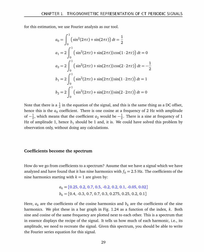
CHAPTER 1. TRIGONOMETRIC REPRESENTATION OF CT PERIODIC SIGNALS
for this estimation, we use Fourier analysis as our tool.
a0 =
∫ 1
0
sin2(2πt) + sin(2πt)
dt=12
a1 = 2
∫ 1
0
sin2(2πt) + sin(2πt)) cos(1 · 2πt)
dt= 0
a2 = 2
∫ 1
0
sin2(2πt) + sin(2πt)) cos(2 · 2πt)
dt= −12
b1 = 2
∫ 1
0
sin2(2πt) + sin(2πt)) sin(1 · 2πt)
dt= 1
b2 = 2
∫ 1
0
sin2(2πt) + sin(2πt)) sin(2 · 2πt)
dt= 0
Note that there is a 12 in the equation of the signal, and this is the same thing as a DC offset,
hence this is the a0 coefficient. There is one cosine at a frequency of 2 Hz with amplitudeof −1
2 , which means that the coefficient a2 would be −12 . There is a sine at frequency of 1
Hz of amplitude 1, hence b1 should be 1 and, it is. We could have solved this problem byobservation only, without doing any calculations.
Coefficients become the spectrum
How do we go from coefficients to a spectrum? Assume that we have a signal which we haveanalyzed and have found that it has nine harmonics with f0 = 2.5 Hz. The coefficients of thenine harmonics starting with k = 1 are given by:
ak = [0.25, 0.2, 0.7, 0.5, -0.2, 0.2, 0.1, -0.05, 0.02]
bk = [0.4, -0.3, 0.7, 0.7, 0.3, 0.275, 0.25, 0.2, 0.1]
Here, ak are the coefficients of the cosine harmonics and bk are the coefficients of the sineharmonics. We plot these in a bar graph in Fig. 1.24 as a function of the index, k. Bothsine and cosine of the same frequency are plotted next to each other. This is a spectrum thatin essence displays the recipe of the signal. It tells us how much of each harmonic, i.e., itsamplitude, we need to recreate the signal. Given this spectrum, you should be able to writethe Fourier series equation for this signal.
29
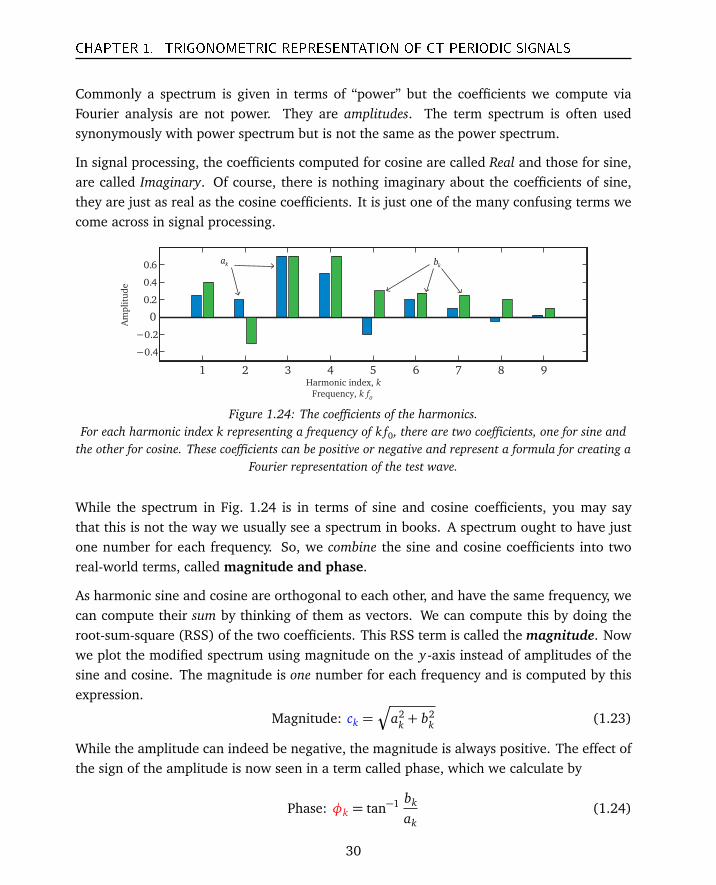
CHAPTER 1. TRIGONOMETRIC REPRESENTATION OF CT PERIODIC SIGNALS
Commonly a spectrum is given in terms of “power” but the coefficients we compute viaFourier analysis are not power. They are amplitudes. The term spectrum is often usedsynonymously with power spectrum but is not the same as the power spectrum.
In signal processing, the coefficients computed for cosine are called Real and those for sine,are called Imaginary. Of course, there is nothing imaginary about the coefficients of sine,they are just as real as the cosine coefficients. It is just one of the many confusing terms wecome across in signal processing.
1 2 3 4 5 6 7 8 9
−0.4
−0.2
0
0.2
0.4
0.6
Harmonic index, k
Frequency, k f0
Amplitude
ka
kb
Figure 1.24: The coefficients of the harmonics.For each harmonic index k representing a frequency of k f0, there are two coefficients, one for sine and
the other for cosine. These coefficients can be positive or negative and represent a formula for creating aFourier representation of the test wave.
While the spectrum in Fig. 1.24 is in terms of sine and cosine coefficients, you may saythat this is not the way we usually see a spectrum in books. A spectrum ought to have justone number for each frequency. So, we combine the sine and cosine coefficients into tworeal-world terms, called magnitude and phase.
As harmonic sine and cosine are orthogonal to each other, and have the same frequency, wecan compute their sum by thinking of them as vectors. We can compute this by doing theroot-sum-square (RSS) of the two coefficients. This RSS term is called the magnitude. Nowwe plot the modified spectrum using magnitude on the y-axis instead of amplitudes of thesine and cosine. The magnitude is one number for each frequency and is computed by thisexpression.
Magnitude: ck =Ç
a2k + b2
k (1.23)
While the amplitude can indeed be negative, the magnitude is always positive. The effect ofthe sign of the amplitude is now seen in a term called phase, which we calculate by
Phase: φk = tan−1 bk
ak(1.24)
30
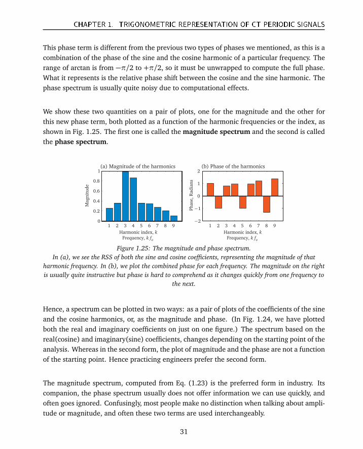
CHAPTER 1. TRIGONOMETRIC REPRESENTATION OF CT PERIODIC SIGNALS
This phase term is different from the previous two types of phases we mentioned, as this is acombination of the phase of the sine and the cosine harmonic of a particular frequency. Therange of arctan is from −π/2 to +π/2, so it must be unwrapped to compute the full phase.What it represents is the relative phase shift between the cosine and the sine harmonic. Thephase spectrum is usually quite noisy due to computational effects.
We show these two quantities on a pair of plots, one for the magnitude and the other forthis new phase term, both plotted as a function of the harmonic frequencies or the index, asshown in Fig. 1.25. The first one is called the magnitude spectrum and the second is calledthe phase spectrum.
1 2 3 4 5 6 7 8 90
0.2
0.4
0.6
0.8
1
Magnitude
1 2 3 4 5 6 7 8 9−2
−1
0
1
2
Phase, Radians
(a) Magnitude of the harmonics (b) Phase of the harmonics
Harmonic index, k
Frequency, k f0
Harmonic index, k
Frequency, k f0
Figure 1.25: The magnitude and phase spectrum.In (a), we see the RSS of both the sine and cosine coefficients, representing the magnitude of that
harmonic frequency. In (b), we plot the combined phase for each frequency. The magnitude on the rightis usually quite instructive but phase is hard to comprehend as it changes quickly from one frequency to
the next.
Hence, a spectrum can be plotted in two ways: as a pair of plots of the coefficients of the sineand the cosine harmonics, or, as the magnitude and phase. (In Fig. 1.24, we have plottedboth the real and imaginary coefficients on just on one figure.) The spectrum based on thereal(cosine) and imaginary(sine) coefficients, changes depending on the starting point of theanalysis. Whereas in the second form, the plot of magnitude and the phase are not a functionof the starting point. Hence practicing engineers prefer the second form.
The magnitude spectrum, computed from Eq. (1.23) is the preferred form in industry. Itscompanion, the phase spectrum usually does not offer information we can use quickly, andoften goes ignored. Confusingly, most people make no distinction when talking about ampli-tude or magnitude, and often these two terms are used interchangeably.
31
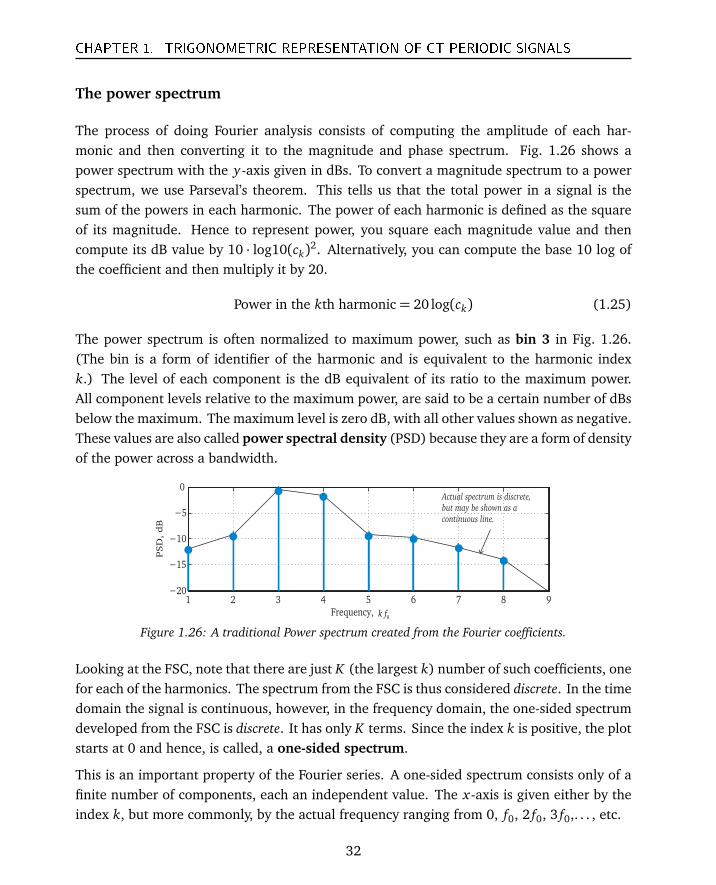
CHAPTER 1. TRIGONOMETRIC REPRESENTATION OF CT PERIODIC SIGNALS
The power spectrum
The process of doing Fourier analysis consists of computing the amplitude of each har-monic and then converting it to the magnitude and phase spectrum. Fig. 1.26 shows apower spectrum with the y-axis given in dBs. To convert a magnitude spectrum to a powerspectrum, we use Parseval’s theorem. This tells us that the total power in a signal is thesum of the powers in each harmonic. The power of each harmonic is defined as the squareof its magnitude. Hence to represent power, you square each magnitude value and thencompute its dB value by 10 · log10(ck)2. Alternatively, you can compute the base 10 log ofthe coefficient and then multiply it by 20.
Power in the kth harmonic= 20 log(ck) (1.25)
The power spectrum is often normalized to maximum power, such as bin 3 in Fig. 1.26.(The bin is a form of identifier of the harmonic and is equivalent to the harmonic indexk.) The level of each component is the dB equivalent of its ratio to the maximum power.All component levels relative to the maximum power, are said to be a certain number of dBsbelow the maximum. The maximum level is zero dB, with all other values shown as negative.These values are also called power spectral density (PSD) because they are a form of densityof the power across a bandwidth.
1 2 3 4 5 6 7 8 9−20
−15
−10
−5
0
0k fFrequency,
PSD, dB
Actual spectrum is discrete,
but may be shown as a
continuous line.
Figure 1.26: A traditional Power spectrum created from the Fourier coefficients.
Looking at the FSC, note that there are just K (the largest k) number of such coefficients, onefor each of the harmonics. The spectrum from the FSC is thus considered discrete. In the timedomain the signal is continuous, however, in the frequency domain, the one-sided spectrumdeveloped from the FSC is discrete. It has only K terms. Since the index k is positive, the plotstarts at 0 and hence, is called, a one-sided spectrum.
This is an important property of the Fourier series. A one-sided spectrum consists only of afinite number of components, each an independent value. The x-axis is given either by theindex k, but more commonly, by the actual frequency ranging from 0, f0, 2 f0, 3 f0,. . . , etc.
32
CHAPTER 1. TRIGONOMETRIC REPRESENTATION OF CT PERIODIC SIGNALS
Fourier analysis applies only to periodic waves. And if that is all we could do with Fourieranalysis, then it would not have a lot of use. For real signals we can never tell what theperiod is nor where it starts. Usually no periodicity can be seen. In fact, a real signal maynot be periodic at all. In this case, further developments of the theory allow us to extend the“period” to infinity so we just pick any section of a signal or even the whole signal and callit “The Period” representing the whole signal. This idea is the basis of the Fourier transformthat we will discuss in Chapter 4.
In this chapter we discussed the Fourier series representation of an arbitrary periodic wavein terms of weighted harmonic sine and cosine waves. In the next chapter, we will look athow we can do the same using the confusing and scary-looking complex exponentials.
Summary of Chapter 1
In this chapter, we introduced the concept of using sinusoids to represent an arbitrary periodicwave. We also introduced the concept of the fundamental frequency and its harmonics. TheFourier series representation consists of finding unique weightings of these harmonics torepresent a particular periodic wave. These weights are called the Fourier series coefficients(FSC). When plotted as a function of frequency, these coefficients represent the spectrum ofthe signal. The spectrum calculated using FSC is discrete although the signal is continuousin time.
Terms used in this chapter:
• Fundamental frequency - The smallest frequency of the signal to be represented byFourier series.
• Harmonic frequencies - All integer multiples of the fundamental frequency.• Sinusoids - Sine or cosine wave.• Harmonic coefficients - The amplitude of a harmonic.• Real and imaginary - Cosine is said to exist in the real plane and sine in the imaginary
plane.• Magnitude - The RSS value of the amplitudes of the sine and cosine of a particular
harmonic. It is always positive.• Phase - The fixed phase shift value of a wave at t = 0, often specified in radians.• One-sided spectrum - A spectrum for positive harmonic index, k = 0, 1, 2, etc.• Power spectrum - Showing distribution of power rather than amplitude.
33
CHAPTER 1. TRIGONOMETRIC REPRESENTATION OF CT PERIODIC SIGNALS
1. The most common trigonometric form of the Fourier series is given by
f (t) = a0 +∞∑
k=1
ak cos(2π fk t) +∞∑
k=1
bk sin(2π fk t)
2. The coefficients of the Fourier series are easily computed by
a0 =1T0
∫ T0
0
f (t) dt
bk =2T0
∫ T0
0
f (t) sin(kω0 t) dt
ak =2T0
∫ T0
0
f (t) cos(kω0 t) dt
3. Many periodic signals can be represented by the weighted sum of harmonics sinusoids.The representation is an estimation and may not be an exact replication.
4. Harmonic sinusoids are orthogonal to each other; hence, the integral of their products(or cross product) is zero.
5. The linearity property of the Fourier series implies that a change of the coefficients ofone harmonic does not affect the coefficients of the other harmonics.
6. A time or phase shift of the signal does not affect the magnitude of the coefficients.7. To synthesize a signal based on the Fourier series, we pick a fundamental frequency
first. All harmonics are integer multiples of the fundamental.8. We designate harmonics by the letter k. Hence, for all integer k, all k f0 frequencies
are harmonics of the fundamental frequency f0.9. Fourier analysis means to find the Fourier coefficients of the Fourier series.
10. The Fourier coefficients are discrete because the harmonics are discrete. Hence thespectrum of a periodic continuous-time signal is discrete.
11. A spectrum can be a spectrum of amplitude, magnitude or power. These are all differentand used for different purposes.
34
CHAPTER 1. TRIGONOMETRIC REPRESENTATION OF CT PERIODIC SIGNALS
Questions
1. Can you state in words the principle behind the Fourier series.2. What is the first and the third harmonic of a sinusoid of frequency 3 Hz?3. Can any signal have harmonics?4. When is one harmonic orthogonal to another? What trigonometric property tells us
that this is true?5. Three non-harmonic sinusoids are added together. What is the period of the summed
wave?6. If we add three non-harmonic sinusoids together, is the resulting signal periodic?7. Is the sum of N harmonics also harmonic to the fundamental?8. Are harmonics within a harmonic set also harmonic to each other?9. If we make the amplitude of a signal, a function of time, what effect will that have on
its frequency?10. A change in phase of a cosine wave means it is still orthogonal to a sine wave of the
same frequency; true or false?11. If the phase of a harmonic is changed, does it remain a harmonic of an another wave?
item If the amplitude of a harmonic is changed, does it remain a harmonic of an anotherwave?
12. What is the maximum amplitude of N harmonic cosine waves added together. What isit for sine waves?
13. We need to represent a wave that starts at time t = 0. What type of harmonics will bein its representation?
14. The summation of odd and even waves can be used to create any waveform we want,true or not?
15. Is Fourier series representation an accurate representation of a wave? Why not?16. Can we create a Fourier series representation of any wave?17. Why do we consider the set of harmonics a basis set? What constitutes a basis set?18. Sine and cosine waves are a basis set for Fourier analysis. Can you give an example of
another set of basis functions.19. What quality of sine and cosine makes them suitable as a basis set?20. Fourier series analysis is considered a linear process. Why?21. What do the coefficients of a Fourier series represent? What does the a0 coefficient
represent?
35
CHAPTER 1. TRIGONOMETRIC REPRESENTATION OF CT PERIODIC SIGNALS
22. What are the Fourier series coefficients of this signal? s = A+ B sin(2π f t).23. We want to compute the FSC of this signal. s = sin(6.5t)− cos(4.75t). What should
we pick as the fundamental frequency so as to accurately represent this signal.24. If the target wave is shifted by a certain phase, what happens to its coefficients?25. How many coefficients would you need to describe this wave? x(t) = 2+ B sin(4πt +
π/2)− cos(12πt). Find the coefficients of this signal.26. What is the fundamental period of this Fourier series representation? x(t) = (1/2)(sin(4πt)+(1/3) sin(12πt) + (1/5) sin(20πt) + (1/7) sin(28πt). What are the coefficients of thefirst four cosine and sine harmonics?
27. Given these equations, what are the Fourier series coefficients, a0, a1, a2 for each case.
(a) y =12+
34
sin(πx)−35
cos(2πx).
(b) y =34
cos(2πx)−35
cos(3πx).
28. What is the difference between amplitude and magnitude?29. The amplitude of a harmonic varies from -1 v to +1 v. What is its peak amplitude
and its peak-to-peak amplitude? What is its magnitude? What is the power of theharmonic? What is the value of the power in dB?
30. Examine Fig. 1.13 and give the first four coefficients of the even square wave.
36
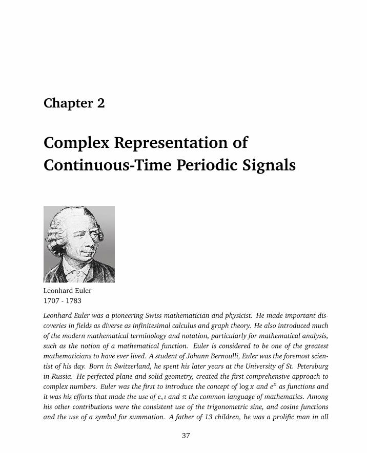
Chapter 2
Complex Representation ofContinuous-Time Periodic Signals
Leonhard Euler1707 - 1783
Leonhard Euler was a pioneering Swiss mathematician and physicist. He made important dis-coveries in fields as diverse as infinitesimal calculus and graph theory. He also introduced muchof the modern mathematical terminology and notation, particularly for mathematical analysis,such as the notion of a mathematical function. Euler is considered to be one of the greatestmathematicians to have ever lived. A student of Johann Bernoulli, Euler was the foremost scien-tist of his day. Born in Switzerland, he spent his later years at the University of St. Petersburgin Russia. He perfected plane and solid geometry, created the first comprehensive approach tocomplex numbers. Euler was the first to introduce the concept of log x and ex as functions andit was his efforts that made the use of e, ı and π the common language of mathematics. Amonghis other contributions were the consistent use of the trigonometric sine, and cosine functionsand the use of a symbol for summation. A father of 13 children, he was a prolific man in all
37
CHAPTER 2. COMPLEX REPRESENTATION OF CONTINUOUS-TIME PERIODIC SIGNALS
aspects, languages, medicine, botany, geography and physical sciences and has left his mark onour scientific thinking.– From Wikipedia
Euler’s Equation
e jωt = cosωt + j sinωt
This equation is called the Euler’s equation. Bertrand Russell and Richard Feynman bothgave this equation plentiful praise with words such as “the most beautiful, profound andsubtle expression in mathematics” and “the most amazing equation in all of mathematics.”This perplexing equation was developed by Euler (pronounced Oiler) in the early 1800s.
The e jωt in Euler’s equation is a decidedly confusing concept. What exactly is the role of j ine jωt? We know from algebra that it stands for
p−1 but what is it doing here with the sine
and cosine? Can we even visualize this function?
The complex exponential
The function e jωt goes by the name of complex exponential (CE). This function is of thegreatest importance in signal processing and Fourier analysis. We are going to discuss itsconceptual nature and its application to Fourier analysis.
e jωt = cosωt + j sinωt (2.1)
Looking at Eq. (2.1), we see the complex exponential on the left side. It is called the positivecomplex exponential, for the simple reason that the exponent of e is positive. On the right ofthe equal sign, underlined, is the expression containing a sine and a cosine. For now, ignorethe complex exponential e jωt on the left-hand side and examine only the right-hand side ofthis equation, containing the sine and cosine waves, with the complex operator j thrown in.
This is a complex function which often means that it is a 3D function. It can be plottedby assigning a particular value to the radial frequency ω, and then for a range of time t,calculating both cosωt and sinωt values. Because the value of ω is held constant, we havethree values, the independent time variable, t, and associated sin and cos values, cos(ωt)and sin(ωt). With these three values, t, cos(ωt) and sin(ωt), we can create the 3D plotshown in Fig. 2.1. Time is plotted on the x-axis, and y and z axis contain the values ofthe function cos(ωt) and sin(ωt). Each plotted helix is for a fixed value of frequency, ω.Changing the frequency will this figure.
38
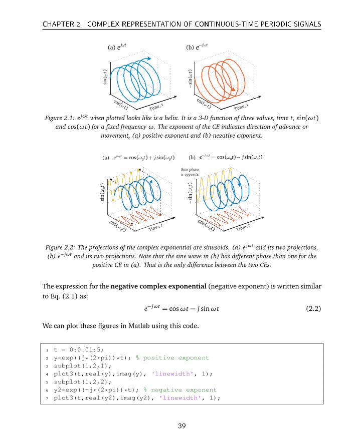
CHAPTER 2. COMPLEX REPRESENTATION OF CONTINUOUS-TIME PERIODIC SIGNALS
Time, tTime, t
j te ω j te ω−
(a) (b)
sin
()t
ω
cos()t
ω
sin
()t
ω−
cos()t
ω
Figure 2.1: e jωt when plotted looks like is a helix. It is a 3-D function of three values, time t, sin(ωt)and cos(ωt) for a fixed frequency ω. The exponent of the CE indicates direction of advance or
movement, (a) positive exponent and (b) negative exponent.
(a) 0
0 0cos( ) sin( )
j te t j tω
ω ω= + (b) 0
0 0cos( ) sin( )
j te t j tω
ω ω−
= −
0
cos()t
ω
0si
n(
)tω
Time, tTime, t
Sine phase
is opposite.
0
cos()t
ω
0si
n(
)tω
Figure 2.2: The projections of the complex exponential are sinusoids. (a) e jωt and its two projections,(b) e− jωt and its two projections. Note that the sine wave in (b) has different phase than one for the
positive CE in (a). That is the only difference between the two CEs.
The expression for the negative complex exponential (negative exponent) is written similarto Eq. (2.1) as:
e− jωt = cosωt − j sinωt (2.2)
We can plot these figures in Matlab using this code.
1 t = 0:0.01:5;2 y=exp((j*(2*pi))*t); % positive exponent3 subplot(1,2,1);4 plot3(t,real(y),imag(y), 'linewidth', 1);5 subplot(1,2,2);6 y2=exp((-j*(2*pi))*t); % negative exponent7 plot3(t,real(y2),imag(y2), 'linewidth', 1);
39
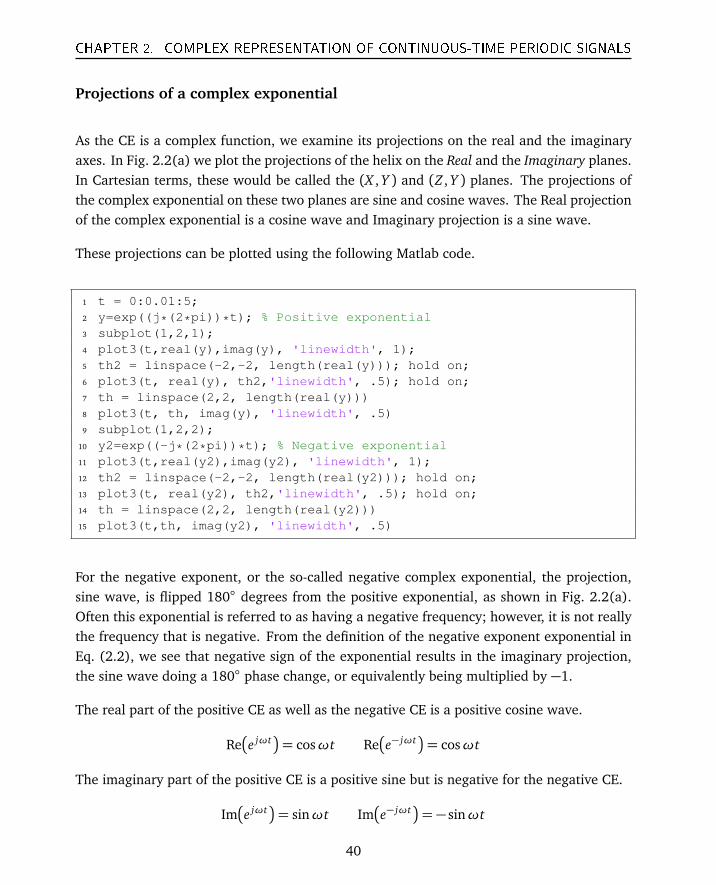
CHAPTER 2. COMPLEX REPRESENTATION OF CONTINUOUS-TIME PERIODIC SIGNALS
Projections of a complex exponential
As the CE is a complex function, we examine its projections on the real and the imaginaryaxes. In Fig. 2.2(a) we plot the projections of the helix on the Real and the Imaginary planes.In Cartesian terms, these would be called the (X , Y ) and (Z , Y ) planes. The projections ofthe complex exponential on these two planes are sine and cosine waves. The Real projectionof the complex exponential is a cosine wave and Imaginary projection is a sine wave.
These projections can be plotted using the following Matlab code.
1 t = 0:0.01:5;2 y=exp((j*(2*pi))*t); % Positive exponential3 subplot(1,2,1);4 plot3(t,real(y),imag(y), 'linewidth', 1);5 th2 = linspace(-2,-2, length(real(y))); hold on;6 plot3(t, real(y), th2,'linewidth', .5); hold on;7 th = linspace(2,2, length(real(y)))8 plot3(t, th, imag(y), 'linewidth', .5)9 subplot(1,2,2);
10 y2=exp((-j*(2*pi))*t); % Negative exponential11 plot3(t,real(y2),imag(y2), 'linewidth', 1);12 th2 = linspace(-2,-2, length(real(y2))); hold on;13 plot3(t, real(y2), th2,'linewidth', .5); hold on;14 th = linspace(2,2, length(real(y2)))15 plot3(t,th, imag(y2), 'linewidth', .5)
For the negative exponent, or the so-called negative complex exponential, the projection,sine wave, is flipped 180 degrees from the positive exponential, as shown in Fig. 2.2(a).Often this exponential is referred to as having a negative frequency; however, it is not reallythe frequency that is negative. From the definition of the negative exponent exponential inEq. (2.2), we see that negative sign of the exponential results in the imaginary projection,the sine wave doing a 180 phase change, or equivalently being multiplied by −1.
The real part of the positive CE as well as the negative CE is a positive cosine wave.
Re
e jωt
= cosωt Re
e− jωt
= cosωt
The imaginary part of the positive CE is a positive sine but is negative for the negative CE.
Im
e jωt
= sinωt Im
e− jωt
= − sinωt
40
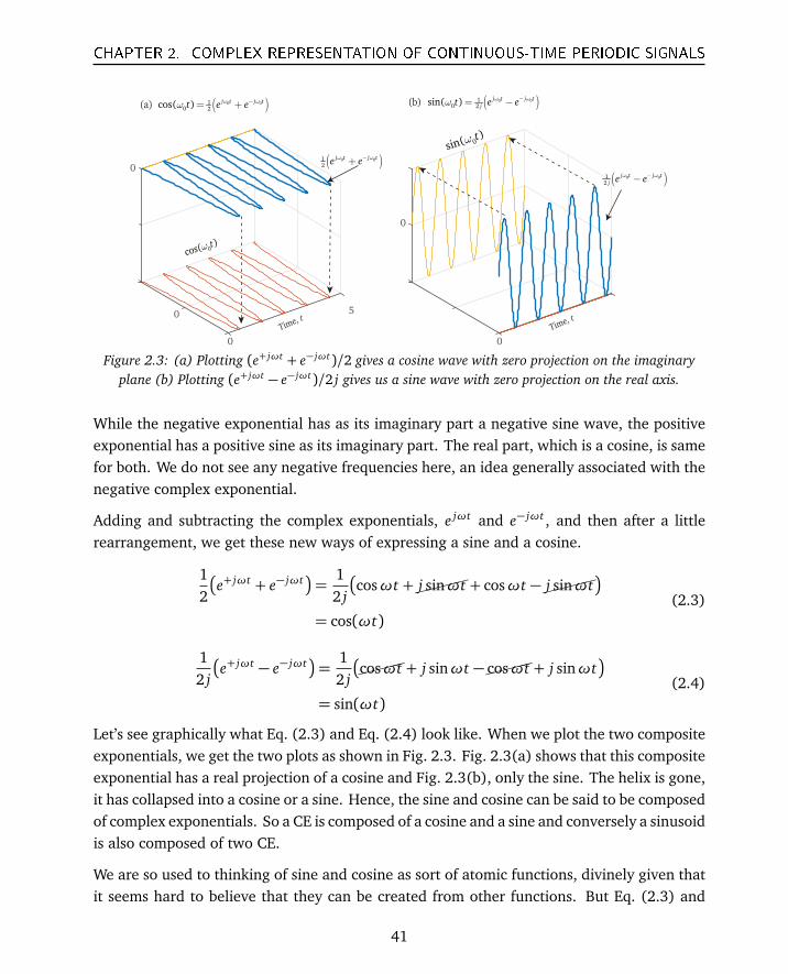
CHAPTER 2. COMPLEX REPRESENTATION OF CONTINUOUS-TIME PERIODIC SIGNALS
50
0
0
0
0
(a) ( )0 01
0 2cos( )
j t j tt e e
ω ω
ω−= +
Time, t
Time, t
0cos(
)tω
0sin
()t
ω
( )0 01
2
j t j te eω ω−+
( )0 01
2
j t j t
je eω ω−−
(b) ( )0 01
0 2sin( )
j t j t
jt e e
ω ω
ω−= −
Figure 2.3: (a) Plotting (e+ jωt + e− jωt)/2 gives a cosine wave with zero projection on the imaginaryplane (b) Plotting (e+ jωt − e− jωt)/2 j gives us a sine wave with zero projection on the real axis.
While the negative exponential has as its imaginary part a negative sine wave, the positiveexponential has a positive sine as its imaginary part. The real part, which is a cosine, is samefor both. We do not see any negative frequencies here, an idea generally associated with thenegative complex exponential.
Adding and subtracting the complex exponentials, e jωt and e− jωt , and then after a littlerearrangement, we get these new ways of expressing a sine and a cosine.
12
e+ jωt + e− jωt
=12 j
cosωt +j sinωt + cosωt −j sinωt
= cos(ωt)(2.3)
12 j
e+ jωt − e− jωt
=12 j
cosωt + j sinωt −cosωt + j sinωt
= sin(ωt)(2.4)
Let’s see graphically what Eq. (2.3) and Eq. (2.4) look like. When we plot the two compositeexponentials, we get the two plots as shown in Fig. 2.3. Fig. 2.3(a) shows that this compositeexponential has a real projection of a cosine and Fig. 2.3(b), only the sine. The helix is gone,it has collapsed into a cosine or a sine. Hence, the sine and cosine can be said to be composedof complex exponentials. So a CE is composed of a cosine and a sine and conversely a sinusoidis also composed of two CE.
We are so used to thinking of sine and cosine as sort of atomic functions, divinely given thatit seems hard to believe that they can be created from other functions. But Eq. (2.3) and
41

CHAPTER 2. COMPLEX REPRESENTATION OF CONTINUOUS-TIME PERIODIC SIGNALS
1 2 3 4 5 7 8
−2
−1
0
1
2
Am
pli
tud
e
x
3
3!
x−
5
5!
x
7
7!
x−
9
9!
x
11
11!
x−
13
13!
x+ + +
sin(x)
Figure 2.4: Sine wave as a sum of many exponentials of different weights.
Eq. (2.4) tell us that both sine and cosine can be created by adding complex exponentials.This is a case of two 3D functions coming together to create a 2D sinusoid.This sounds strangebut it’s actually not an unfamiliar concept. We can add two 2D functions and get a 1Dfunction. An example is when we add a sine and a 180 shifted sine, we get a straight line,a 1D function. So a 2D function created by two 3D functions should not be a big stumblingblock.
The Sinusoids
So how did Euler’s equation come about and why is it so important to signal processing? Wewill try to answer that by first looking at Taylor series representations of the exponential ex ,sines, and the cosines. The Taylor series expansion for the two sinusoids is given in 2D bythe infinite series as:
cos x = 1−x2
2!+
x4
4!−
x6
6!+ . . .
sin x = x −x3
3!+
x5
5!−
x7
7!+ . . .
(2.5)
Note that each one of these series is composed of many individual exponential functions.Thus, sine waves really are composed of exponentials! However, these are real exponentialsthat are nonperiodic and not the same thing as the complex exponentials. Complex expo-nentials are a special class of real exponentials and are used as an alternate to the sinusoidsin Fourier analysis, as they are periodic and offer ease of expression and calculation, whichis not obvious when we encounter them at first.
Real exponentials are used in Laplace analysis as the basis set, instead of the complex expo-nentials we use in Fourier analysis. Real exponentials are more general than complex expo-
42
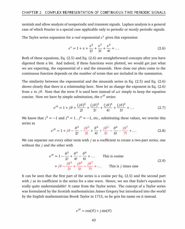
CHAPTER 2. COMPLEX REPRESENTATION OF CONTINUOUS-TIME PERIODIC SIGNALS
nentials and allow analysis of nonperiodic and transient signals. Laplace analysis is a generalcase of which Fourier is a special case applicable only to periodic or mostly periodic signals.
The Taylor series expansion for a real exponential ex gives this expression
ex = 1+ x +x2
2!+
x3
3!+
x4
4!+ . . . (2.6)
Both of these equations, Eq. (2.5) and Eq. (2.6) are straightforward concepts after you havedigested them a bit. And indeed, if these functions were plotted, we would get just whatwe are expecting, the exponential of e and the sinusoids. How close our plots come to thecontinuous function depends on the number of terms that are included in the summation.
The similarity between the exponential and the sinusoids series in Eq. (2.5) and Eq. (2.6)shows clearly that there is a relationship here. Now let us change the exponent in Eq. (2.6)from x to jθ . Note that the term θ is used here instead of ωt simply to keep the equationconcise. Now we have by simple substitution, the e jθ series:
e jθ = 1+ jθ +( jθ )2
2!+( jθ )3
3!+( jθ )4
4!+( jθ )5
5!+ . . . (2.7)
We know that j2 = −1 and j4 = 1 , j6 = −1, etc., substituting these values, we rewrite thisseries as
e jθ = 1+ jθ −θ2
2!−
jθ3
3!+θ4
4!+
jθ5
5!−θ6
6!−
jθ7
7!+ . . . (2.8)
We can separate out every other term with j as a coefficient to create a two-part series, onewithout the j and the other with
e jθ = 1−θ2
2!+θ4
4!−θ6
6!+ . . . This is cosine
+ jθ −jθ3
3!+
jθ5
5!−
jθ7
7!+ . . . This is j times sine
(2.9)
It can be seen that the first part of the series is a cosine per Eq. (2.5) and the second partwith j as its coefficient is the series for a sine wave. Hence, we see that Euler’s equation isreally quite understandable! It came from the Taylor series. The concept of a Taylor serieswas formulated by the Scottish mathematician James Gregory but introduced into the worldby the English mathematician Brook Taylor in 1715, so he gets his name on it instead.
e jθ = cos(θ ) + j sin(θ )
43
CHAPTER 2. COMPLEX REPRESENTATION OF CONTINUOUS-TIME PERIODIC SIGNALS
We can now derive some interesting results from the Euler’s equation, such as the following.By setting θ = π/2, we can show that
e jπ/2 =cos(π/2) + j sin(π/2)
= 0+ j · 1
= j
By setting θ = 3π/2, we can show that
e j3π/2 =cos(3π/2) + j sin(3π/2)
= 0+ j · −1
= − j
And an another interesting result:
e jπ = cos(π) + j sin(π) = −1
From this, we can write this amazing looking equation!
e jπ + 1= 0
So this complex looking function is not so complicated after all. These are some of the usefulproperties of a CE that we will be using. The function maintains a wondrous and mysteriousquality, with added tinge of fear for some. However, we need to get over our fear of thisequation and learn to love it. But, the question now is why bring up the Euler’s equationin context of Fourier analysis at all? Why all this rigmarole about the complex exponential,why are sines and cosines not good enough? They are certainly easier to visualize.
In Fourier analysis, we computed the coefficients of sines and cosines (the harmonics) sepa-rately. In Chapter 1, we discussed the three different formulations of the Fourier series usingsines and cosines, only with cosines, and with complex exponentials. Fourier analysis usingthe trigonometric form is not easy in practice. Trig functions are easy to understand but hardto manipulate. In fact, adding and multiplying them is a pain. On the other hand, doingmath with exponentials is considerably easier. (See examples in Appendix A.)
Using a single exponential representing both sinusoids can simplify calculations in Fourierseries. This is the main advantage of switching to complex exponentials in using the complexform of the Fourier series. The math looks hard but is actually easier. However, complex
44

CHAPTER 2. COMPLEX REPRESENTATION OF CONTINUOUS-TIME PERIODIC SIGNALS
exponentials bring with them some conceptual difficulties, which is that they are hard tovisualize and are confusing at first.
Typically, when we decompose something, we do it into a simpler form but here seemingly amore complex form is being employed. A simpler quantity, a cosine wave is now decomposedinto two complex functions. However, the net result is that it will make Fourier analysissimpler. We will go from simplicity to complexity and then to simplicity again.
Let us take this sinusoid that has a phase term to complicate things and present it in complexform.
x(t) = Acos(ωt + θ )
=A2
e j(ωt+θ ) +A2
e− j(ωt+θ )
=A2
e jωt e jθ +A2
e− jωt e− jθ
In the last row, we separate the exponential into its powers. If we expand this expressioninto trigonometric domain using Euler’s equation, we see that indeed we do get back thetrigonometric cosine wave we started with.
=A2
cos(ωt + θ ) +(((((((j sin(ωt + θ ) + cos(ωt + θ )−(((((
((j sin(ωt + θ )
= Acos(ωt + θ )
Fourier Series Representation using Complex Exponentials
In Chapter 1, we used trigonometric harmonics (the sine and cosine) as a basis set to developthe Fourier series representation. The target signal was “mapped” onto a k set of sinusoidalharmonics, such as these based on fundamental frequency of ω0.
S =
sinω0 t, cosω0 t, sin2ω0 t, cos 2ω0 t, . . . , cos kω0 t, . . . ,
A set of complex exponentials given by set S, can then be used alternately as a basis set forcreating a complex (but preferred) form of the Fourier series.
S =
. . . , e−3 jω0 t , e−2 jω0 t , e−1 jω0 t , 1 , e1 jω0 t , . . . , ek jω0 t , . . .
The big difference between these two forms is that whereas for the trigonometric form, theindex k is strictly positive, for the complex exponential form, it covers both positive and
45
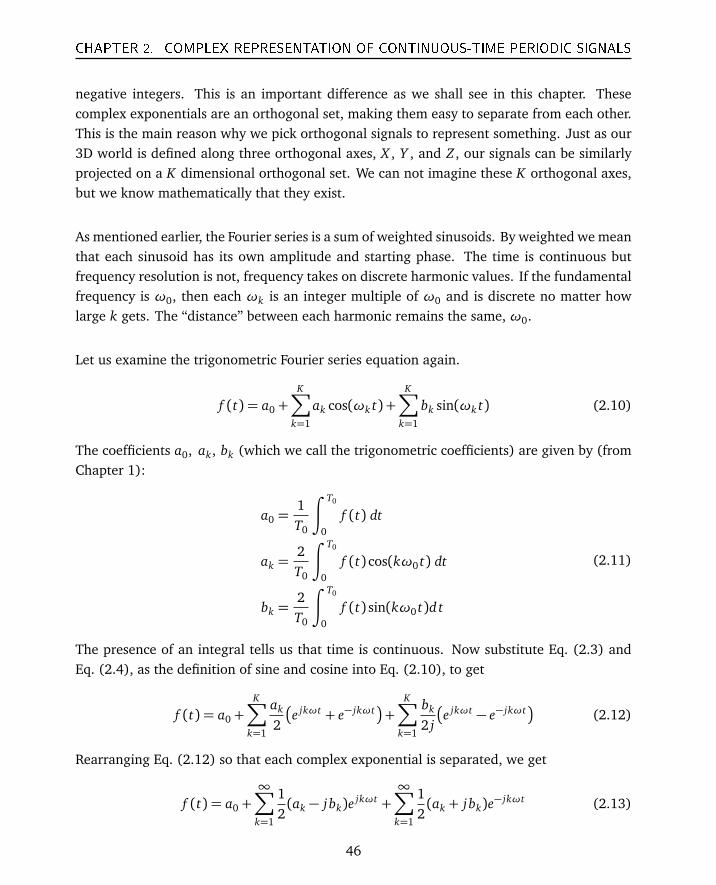
CHAPTER 2. COMPLEX REPRESENTATION OF CONTINUOUS-TIME PERIODIC SIGNALS
negative integers. This is an important difference as we shall see in this chapter. Thesecomplex exponentials are an orthogonal set, making them easy to separate from each other.This is the main reason why we pick orthogonal signals to represent something. Just as our3D world is defined along three orthogonal axes, X , Y , and Z , our signals can be similarlyprojected on a K dimensional orthogonal set. We can not imagine these K orthogonal axes,but we know mathematically that they exist.
As mentioned earlier, the Fourier series is a sum of weighted sinusoids. By weighted we meanthat each sinusoid has its own amplitude and starting phase. The time is continuous butfrequency resolution is not, frequency takes on discrete harmonic values. If the fundamentalfrequency is ω0, then each ωk is an integer multiple of ω0 and is discrete no matter howlarge k gets. The “distance” between each harmonic remains the same, ω0.
Let us examine the trigonometric Fourier series equation again.
f (t) = a0 +K∑
k=1
ak cos(ωk t) +K∑
k=1
bk sin(ωk t) (2.10)
The coefficients a0, ak, bk (which we call the trigonometric coefficients) are given by (fromChapter 1):
a0 =1T0
∫ T0
0
f (t) dt
ak =2T0
∫ T0
0
f (t) cos(kω0 t) dt
bk =2T0
∫ T0
0
f (t) sin(kω0 t)d t
(2.11)
The presence of an integral tells us that time is continuous. Now substitute Eq. (2.3) andEq. (2.4), as the definition of sine and cosine into Eq. (2.10), to get
f (t) = a0 +K∑
k=1
ak
2
e jkωt + e− jkωt
+K∑
k=1
bk
2 j
e jkωt − e− jkωt
(2.12)
Rearranging Eq. (2.12) so that each complex exponential is separated, we get
f (t) = a0 +∞∑
k=1
12(ak − j bk)e
jkωt +∞∑
k=1
12(ak + j bk)e
− jkωt (2.13)
46
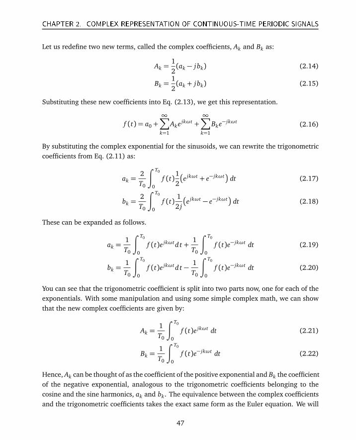
CHAPTER 2. COMPLEX REPRESENTATION OF CONTINUOUS-TIME PERIODIC SIGNALS
Let us redefine two new terms, called the complex coefficients, Ak and Bk as:
Ak =12(ak − j bk) (2.14)
Bk =12(ak + j bk) (2.15)
Substituting these new coefficients into Eq. (2.13), we get this representation.
f (t) = a0 +∞∑
k=1
Ake jkωt +∞∑
k=1
Bke− jkωt (2.16)
By substituting the complex exponential for the sinusoids, we can rewrite the trigonometriccoefficients from Eq. (2.11) as:
ak =2T0
∫ T0
0
f (t)12
e jkωt + e− jkωt
dt (2.17)
bk =2T0
∫ T0
0
f (t)12 j
e jkωt − e− jkωt
dt (2.18)
These can be expanded as follows.
ak =1T0
∫ T0
0
f (t)e jkωt d t +1T0
∫ T0
0
f (t)e− jkωt dt (2.19)
bk =1T0
∫ T0
0
f (t)e jkωt d t −1T0
∫ T0
0
f (t)e− jkωt dt (2.20)
You can see that the trigonometric coefficient is split into two parts now, one for each of theexponentials. With some manipulation and using some simple complex math, we can showthat the new complex coefficients are given by:
Ak =1T0
∫ T0
0
f (t)e jkωt dt (2.21)
Bk =1T0
∫ T0
0
f (t)e− jkωt dt (2.22)
Hence, Ak can be thought of as the coefficient of the positive exponential and Bk the coefficientof the negative exponential, analogous to the trigonometric coefficients belonging to thecosine and the sine harmonics, ak and bk. The equivalence between the complex coefficientsand the trigonometric coefficients takes the exact same form as the Euler equation. We will
47
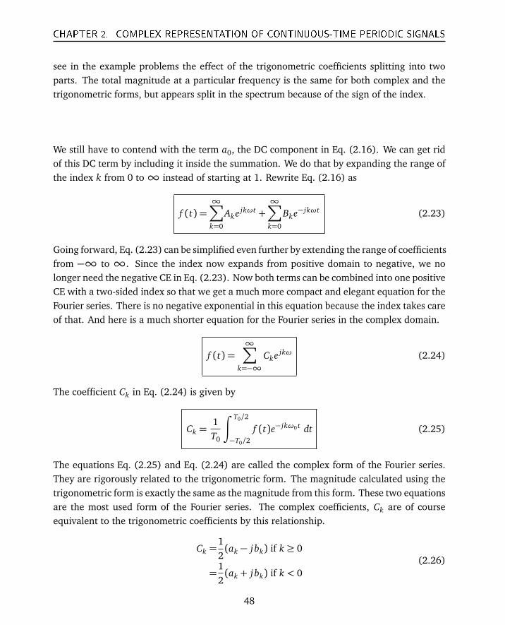
CHAPTER 2. COMPLEX REPRESENTATION OF CONTINUOUS-TIME PERIODIC SIGNALS
see in the example problems the effect of the trigonometric coefficients splitting into twoparts. The total magnitude at a particular frequency is the same for both complex and thetrigonometric forms, but appears split in the spectrum because of the sign of the index.
We still have to contend with the term a0, the DC component in Eq. (2.16). We can get ridof this DC term by including it inside the summation. We do that by expanding the range ofthe index k from 0 to∞ instead of starting at 1. Rewrite Eq. (2.16) as
f (t) =∞∑
k=0
Ake jkωt +∞∑
k=0
Bke− jkωt (2.23)
Going forward, Eq. (2.23) can be simplified even further by extending the range of coefficientsfrom −∞ to ∞. Since the index now expands from positive domain to negative, we nolonger need the negative CE in Eq. (2.23). Now both terms can be combined into one positiveCE with a two-sided index so that we get a much more compact and elegant equation for theFourier series. There is no negative exponential in this equation because the index takes careof that. And here is a much shorter equation for the Fourier series in the complex domain.
f (t) =∞∑
k=−∞Cke jkω (2.24)
The coefficient Ck in Eq. (2.24) is given by
Ck =1T0
∫ T0/2
−T0/2
f (t)e− jkω0 t dt (2.25)
The equations Eq. (2.25) and Eq. (2.24) are called the complex form of the Fourier series.They are rigorously related to the trigonometric form. The magnitude calculated using thetrigonometric form is exactly the same as the magnitude from this form. These two equationsare the most used form of the Fourier series. The complex coefficients, Ck are of courseequivalent to the trigonometric coefficients by this relationship.
Ck =12(ak − j bk) if k ≥ 0
=12(ak + j bk) if k < 0
(2.26)
48
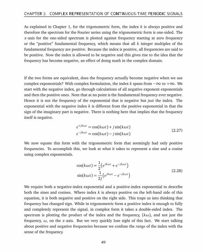
CHAPTER 2. COMPLEX REPRESENTATION OF CONTINUOUS-TIME PERIODIC SIGNALS
As explained in Chapter 1, for the trigonometric form, the index k is always positive andtherefore the spectrum for the Fourier series using the trigonometric form is one-sided. Thex-axis for the one-sided spectrum is plotted against frequency starting at zero frequencyor the “positive” fundamental frequency, which means that all k integer multiples of thefundamental frequency are positive. Because the index is positive, all frequencies are said tobe positive. Now the index is allowed to be negative and this gives rise to the idea that thefrequency has become negative, an effect of doing math in the complex domain.
If the two forms are equivalent, does the frequency actually become negative when we usecomplex exponentials? With complex formulation, the index k spans from −∞ to +∞. Westart with the negative index, go through calculations of all negative exponent exponentialsand then the positive ones. Note that at no point is the fundamental frequency ever negative.Hence it is not the frequency of the exponential that is negative but just the index. Theexponential with the negative index k is different from the positive exponential in that thesign of the imaginary part is negative. There is nothing here that implies that the frequencyitself is negative.
e+ jkωt = cos(kωt) + j sin(kωt)
e− jkωt = cos(kωt)− j sin(kωt)(2.27)
We now equate this form with the trigonometric form that seemingly had only positivefrequencies. To accomplish this, we look at what it takes to represent a sine and a cosineusing complex exponentials.
cos(kωt) =12
e jkωt + e− jkωt
sin(kωt) =12 j
e jkωt − e− jkωt
(2.28)
We require both a negative-index exponential and a positive-index exponential to describeboth the sines and cosines. Where index k is always positive on the left-hand side of thisequation, it is both negative and positive on the right side. This traps us into thinking thatfrequency has changed sign. While in trigonometric form a positive index is enough to fullyand completely represent the signal, in complex form it takes a double-sided index. Thespectrum is plotting the product of the index and the frequency, (kω), and not just thefrequency, ω, on the x-axis. But we very quickly lose sight of this fact. We start talkingabout positive and negative frequencies because we confuse the range of the index with thesense of the frequency.
49
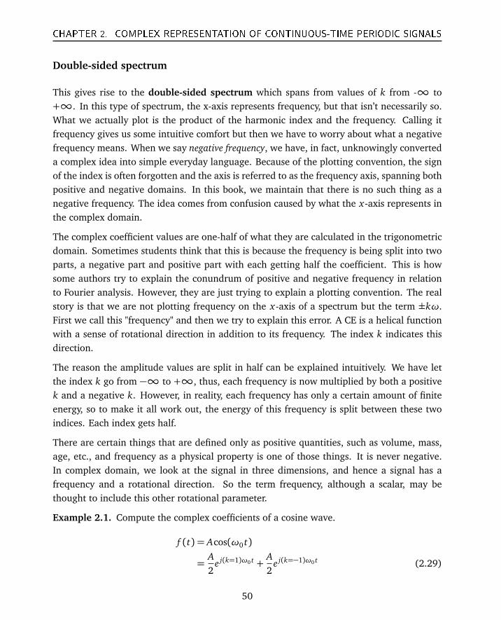
CHAPTER 2. COMPLEX REPRESENTATION OF CONTINUOUS-TIME PERIODIC SIGNALS
Double-sided spectrum
This gives rise to the double-sided spectrum which spans from values of k from -∞ to+∞. In this type of spectrum, the x-axis represents frequency, but that isn’t necessarily so.What we actually plot is the product of the harmonic index and the frequency. Calling itfrequency gives us some intuitive comfort but then we have to worry about what a negativefrequency means. When we say negative frequency, we have, in fact, unknowingly converteda complex idea into simple everyday language. Because of the plotting convention, the signof the index is often forgotten and the axis is referred to as the frequency axis, spanning bothpositive and negative domains. In this book, we maintain that there is no such thing as anegative frequency. The idea comes from confusion caused by what the x-axis represents inthe complex domain.
The complex coefficient values are one-half of what they are calculated in the trigonometricdomain. Sometimes students think that this is because the frequency is being split into twoparts, a negative part and positive part with each getting half the coefficient. This is howsome authors try to explain the conundrum of positive and negative frequency in relationto Fourier analysis. However, they are just trying to explain a plotting convention. The realstory is that we are not plotting frequency on the x-axis of a spectrum but the term ±kω.First we call this "frequency" and then we try to explain this error. A CE is a helical functionwith a sense of rotational direction in addition to its frequency. The index k indicates thisdirection.
The reason the amplitude values are split in half can be explained intuitively. We have letthe index k go from −∞ to +∞, thus, each frequency is now multiplied by both a positivek and a negative k. However, in reality, each frequency has only a certain amount of finiteenergy, so to make it all work out, the energy of this frequency is split between these twoindices. Each index gets half.
There are certain things that are defined only as positive quantities, such as volume, mass,age, etc., and frequency as a physical property is one of those things. It is never negative.In complex domain, we look at the signal in three dimensions, and hence a signal has afrequency and a rotational direction. So the term frequency, although a scalar, may bethought to include this other rotational parameter.
Example 2.1. Compute the complex coefficients of a cosine wave.
f (t) = Acos(ω0 t)
=A2
e j(k=1)ω0 t +A2
e j(k=−1)ω0 t (2.29)
50
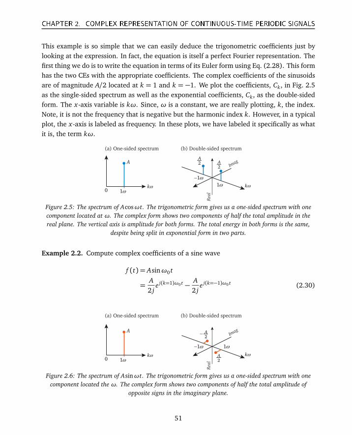
CHAPTER 2. COMPLEX REPRESENTATION OF CONTINUOUS-TIME PERIODIC SIGNALS
This example is so simple that we can easily deduce the trigonometric coefficients just bylooking at the expression. In fact, the equation is itself a perfect Fourier representation. Thefirst thing we do is to write the equation in terms of its Euler form using Eq. (2.28). This formhas the two CEs with the appropriate coefficients. The complex coefficients of the sinusoidsare of magnitude A/2 located at k = 1 and k = −1. We plot the coefficients, Ck, in Fig. 2.5as the single-sided spectrum as well as the exponential coefficients, Ck, as the double-sidedform. The x-axis variable is kω. Since, ω is a constant, we are really plotting, k, the index.Note, it is not the frequency that is negative but the harmonic index k. However, in a typicalplot, the x-axis is labeled as frequency. In these plots, we have labeled it specifically as whatit is, the term kω.
kω
A2A
kω
1ω−
1ω
1ω0
Rea
l
Imag2
A
(a) One-sided spectrum (b) Double-sided spectrum
Figure 2.5: The spectrum of Acosωt. The trigonometric form gives us a one-sided spectrum with onecomponent located at ω. The complex form shows two components of half the total amplitude in thereal plane. The vertical axis is amplitude for both forms. The total energy in both forms is the same,
despite being split in exponential form in two parts.
Example 2.2. Compute complex coefficients of a sine wave
f (t) = Asinω0 t
=A2 j
e j(k=1)ω0 t −A2 j
e j(k=−1)ω0 t (2.30)
kω
A
2A kω
1ω− 1ω
1ω0
Rea
l
Imag
2A
(a) One-sided spectrum (b) Double-sided spectrum
Figure 2.6: The spectrum of Asinωt. The trigonometric form gives us a one-sided spectrum with onecomponent located the ω. The complex form shows two components of half the total amplitude of
opposite signs in the imaginary plane.
51
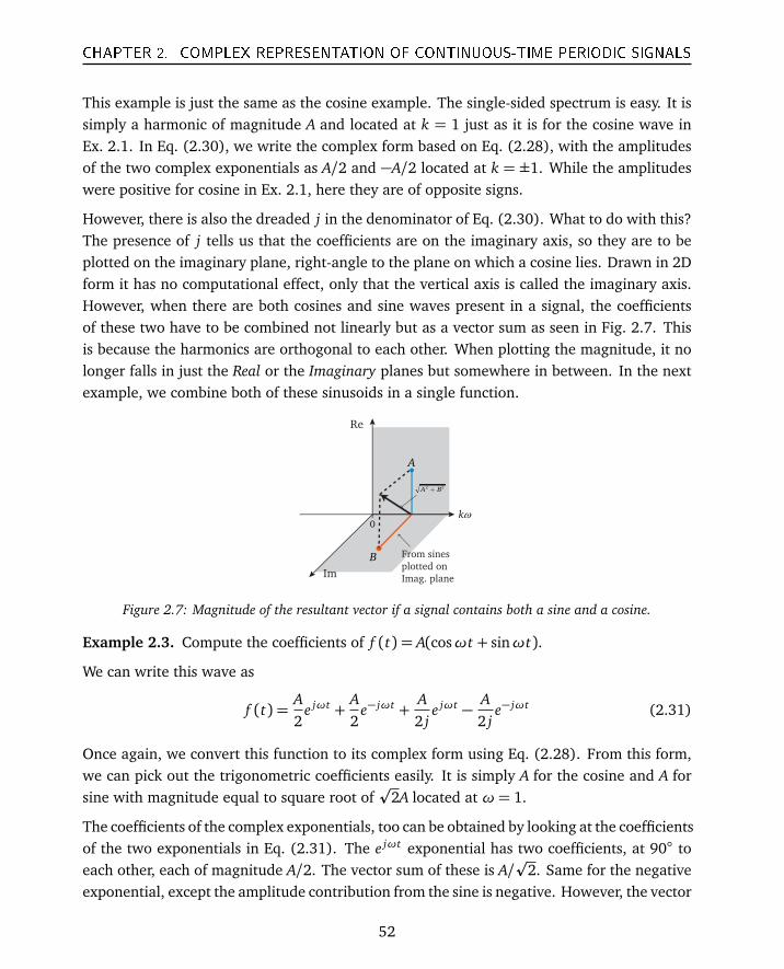
CHAPTER 2. COMPLEX REPRESENTATION OF CONTINUOUS-TIME PERIODIC SIGNALS
This example is just the same as the cosine example. The single-sided spectrum is easy. It issimply a harmonic of magnitude A and located at k = 1 just as it is for the cosine wave inEx. 2.1. In Eq. (2.30), we write the complex form based on Eq. (2.28), with the amplitudesof the two complex exponentials as A/2 and −A/2 located at k = ±1. While the amplitudeswere positive for cosine in Ex. 2.1, here they are of opposite signs.
However, there is also the dreaded j in the denominator of Eq. (2.30). What to do with this?The presence of j tells us that the coefficients are on the imaginary axis, so they are to beplotted on the imaginary plane, right-angle to the plane on which a cosine lies. Drawn in 2Dform it has no computational effect, only that the vertical axis is called the imaginary axis.However, when there are both cosines and sine waves present in a signal, the coefficientsof these two have to be combined not linearly but as a vector sum as seen in Fig. 2.7. Thisis because the harmonics are orthogonal to each other. When plotting the magnitude, it nolonger falls in just the Real or the Imaginary planes but somewhere in between. In the nextexample, we combine both of these sinusoids in a single function.
kω0
Re
Im
From sines
plotted on
Imag. plane
A
B
2 2A B+
Figure 2.7: Magnitude of the resultant vector if a signal contains both a sine and a cosine.
Example 2.3. Compute the coefficients of f (t) = A(cosωt + sinωt).
We can write this wave as
f (t) =A2
e jωt +A2
e− jωt +A2 j
e jωt −A2 j
e− jωt (2.31)
Once again, we convert this function to its complex form using Eq. (2.28). From this form,we can pick out the trigonometric coefficients easily. It is simply A for the cosine and A forsine with magnitude equal to square root of
p2A located at ω= 1.
The coefficients of the complex exponentials, too can be obtained by looking at the coefficientsof the two exponentials in Eq. (2.31). The e jωt exponential has two coefficients, at 90 toeach other, each of magnitude A/2. The vector sum of these is A/
p2. Same for the negative
exponential, except the amplitude contribution from the sine is negative. However, the vector
52
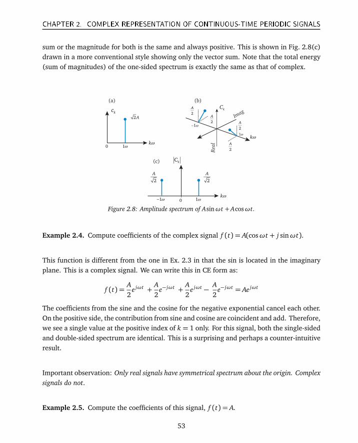
CHAPTER 2. COMPLEX REPRESENTATION OF CONTINUOUS-TIME PERIODIC SIGNALS
sum or the magnitude for both is the same and always positive. This is shown in Fig. 2.8(c)drawn in a more conventional style showing only the vector sum. Note that the total energy(sum of magnitudes) of the one-sided spectrum is exactly the same as that of complex.
1ωkω
0
kω
0
2A
(a)
(c)
kω
1ω−
1ω
kC
Rea
l
Imag
Ck
(b)
1ω− 1ω
2
A
2
A
kc
2
A
2
A
2
A
2
A
Figure 2.8: Amplitude spectrum of Asinωt + Acosωt.
Example 2.4. Compute coefficients of the complex signal f (t) = A(cosωt + j sinωt).
This function is different from the one in Ex. 2.3 in that the sin is located in the imaginaryplane. This is a complex signal. We can write this in CE form as:
f (t) =A2
e jωt +A2
e− jωt +A2
e jωt −A2
e− jωt = Ae jωt
The coefficients from the sine and the cosine for the negative exponential cancel each other.On the positive side, the contribution from sine and cosine are coincident and add. Therefore,we see a single value at the positive index of k = 1 only. For this signal, both the single-sidedand double-sided spectrum are identical. This is a surprising and perhaps a counter-intuitiveresult.
Important observation: Only real signals have symmetrical spectrum about the origin. Complexsignals do not.
Example 2.5. Compute the coefficients of this signal, f (t) = A.
53
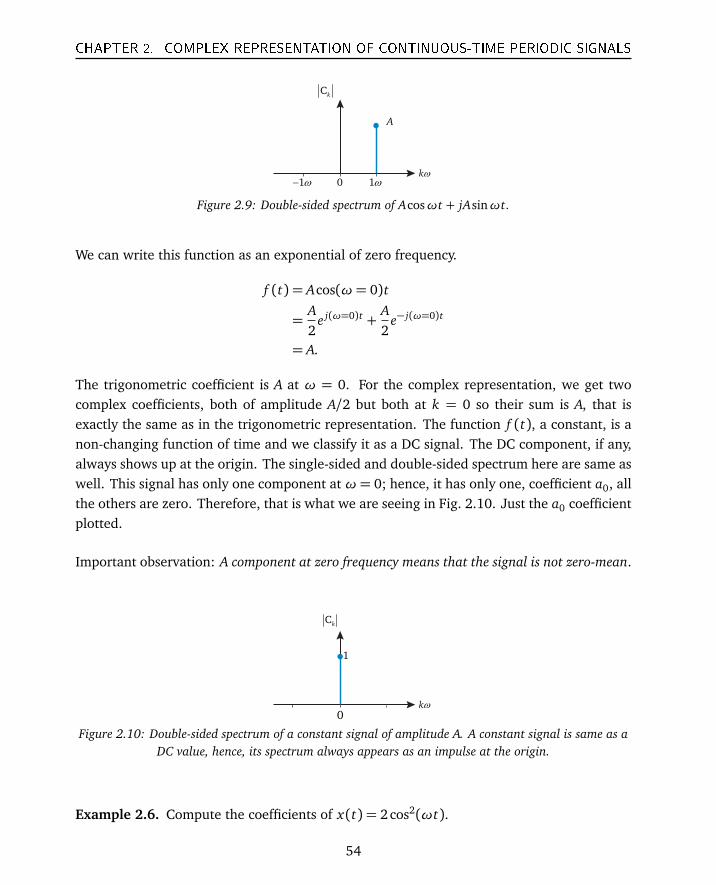
CHAPTER 2. COMPLEX REPRESENTATION OF CONTINUOUS-TIME PERIODIC SIGNALS
kω
1ω1ω− 0
Ck
A
Figure 2.9: Double-sided spectrum of Acosωt + jAsinωt.
We can write this function as an exponential of zero frequency.
f (t) = Acos(ω= 0)t
=A2
e j(ω=0)t +A2
e− j(ω=0)t
= A.
The trigonometric coefficient is A at ω = 0. For the complex representation, we get twocomplex coefficients, both of amplitude A/2 but both at k = 0 so their sum is A, that isexactly the same as in the trigonometric representation. The function f (t), a constant, is anon-changing function of time and we classify it as a DC signal. The DC component, if any,always shows up at the origin. The single-sided and double-sided spectrum here are same aswell. This signal has only one component at ω= 0; hence, it has only one, coefficient a0, allthe others are zero. Therefore, that is what we are seeing in Fig. 2.10. Just the a0 coefficientplotted.
Important observation: A component at zero frequency means that the signal is not zero-mean.
0
kω
1
Ck
Figure 2.10: Double-sided spectrum of a constant signal of amplitude A. A constant signal is same as aDC value, hence, its spectrum always appears as an impulse at the origin.
Example 2.6. Compute the coefficients of x(t) = 2cos2(ωt).
54
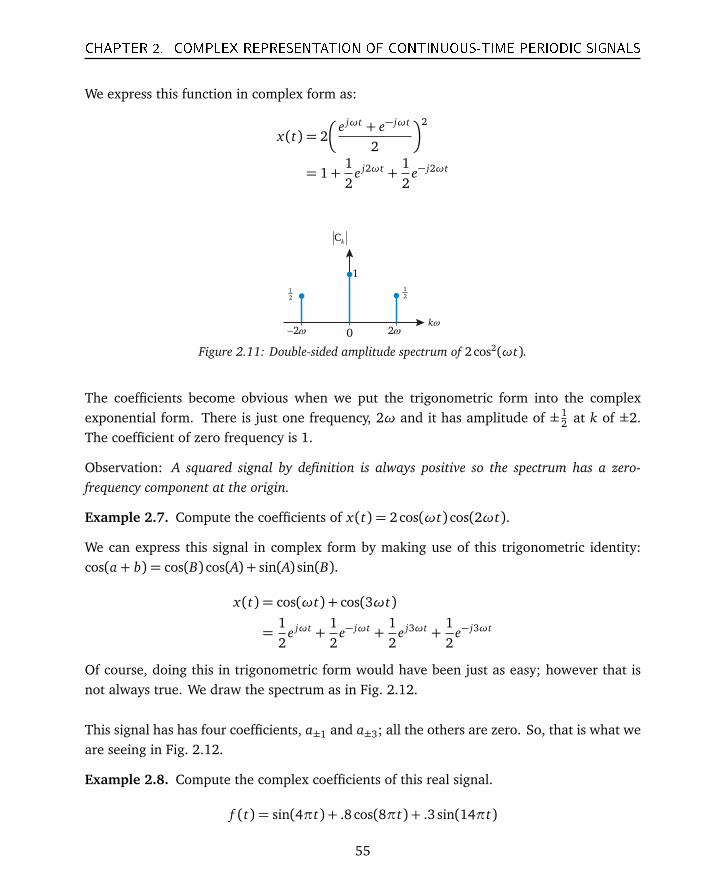
CHAPTER 2. COMPLEX REPRESENTATION OF CONTINUOUS-TIME PERIODIC SIGNALS
We express this function in complex form as:
x(t) = 2
e jωt + e− jωt
2
2
= 1+12
e j2ωt +12
e− j2ωt
0
kω
1
1
2
1
2
2ω− 2ω
Ck
Figure 2.11: Double-sided amplitude spectrum of 2 cos2(ωt).
The coefficients become obvious when we put the trigonometric form into the complexexponential form. There is just one frequency, 2ω and it has amplitude of ±1
2 at k of ±2.The coefficient of zero frequency is 1.
Observation: A squared signal by definition is always positive so the spectrum has a zero-frequency component at the origin.
Example 2.7. Compute the coefficients of x(t) = 2 cos(ωt) cos(2ωt).
We can express this signal in complex form by making use of this trigonometric identity:cos(a+ b) = cos(B) cos(A) + sin(A) sin(B).
x(t) = cos(ωt) + cos(3ωt)
=12
e jωt +12
e− jωt +12
e j3ωt +12
e− j3ωt
Of course, doing this in trigonometric form would have been just as easy; however that isnot always true. We draw the spectrum as in Fig. 2.12.
This signal has has four coefficients, a±1 and a±3; all the others are zero. So, that is what weare seeing in Fig. 2.12.
Example 2.8. Compute the complex coefficients of this real signal.
f (t) = sin(4πt) + .8 cos(8πt) + .3 sin(14πt)
55

CHAPTER 2. COMPLEX REPRESENTATION OF CONTINUOUS-TIME PERIODIC SIGNALS
kω
1
2
1
2
1ω− 1ω
1
2
1
2
3ω2ω2ω−3ω−4ω− 4ω0
Ck
Figure 2.12: Double-sided amplitude spectrum of 2cos(ωt) cos(2ωt).
We want all these frequencies to fall on a harmonic, so we select as the fundamental frequency,f = 1. The signal has six components, at k = ±2,±4,±7. We can write this equation incomplex form as:
f (t) =12
e j2π(k=2)t +12
e j2π(k=−2)t
+0.82
e j2π(k=4)t +0.82 j
e j2π(k=−4)t
+0.32 j
e j2π(k=7)t +0.32
e j2π(k=−7)t
The contributions at k = 2 comes only from a sine, at k = 4 from a cosine and at k = 7 onlyfrom a sine. Note, we plot these on the same line at full magnitude as if j does not exist inthe equation. (We will drop mentioning the index k and call it frequency to fall in line withcommon usage. However, note that it is this sloppiness in terms that causes us to questionour sanity and start asking: what is a negative frequency?)
kω
2ω− 2ω 4ω4ω−7ω− 7ω0
.5
.4
.15
.5
.4
.15
Ck
Figure 2.13: Two-sided symmetrical magnitude spectrum.
This signal has six coefficients, a±2, a±4 and a±7. All the others are zero. So that is what weare seeing here in Fig. 2.13. Just those three coefficients plotted on each side, with half theamplitudes from the time domain equation.
Example 2.9. Compute the complex coefficients of this real signal with phase terms. Thencompute its power spectrum.
x(t) = 3+ 6 cos(4πt + 2) + j sin(4πt + 3)− j6 sin(10πt + 1.5)
56
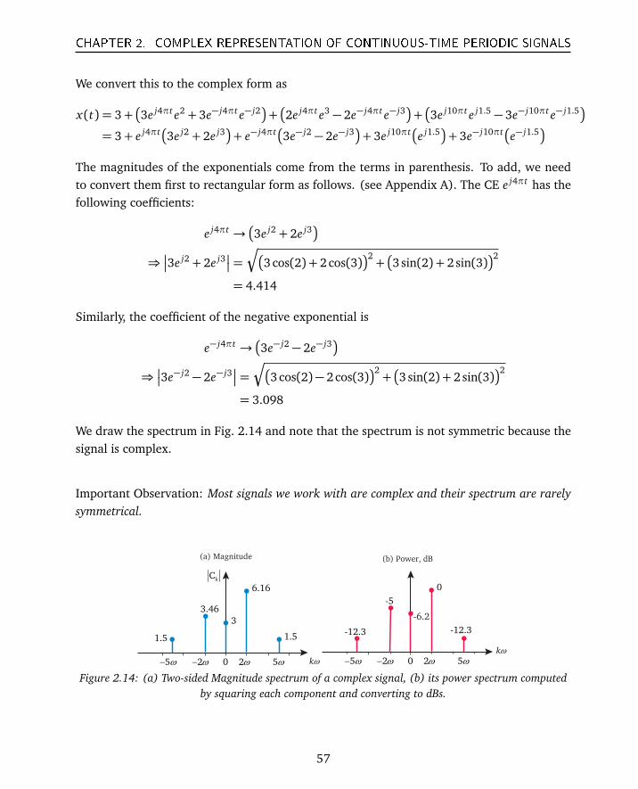
CHAPTER 2. COMPLEX REPRESENTATION OF CONTINUOUS-TIME PERIODIC SIGNALS
We convert this to the complex form as
x(t) = 3+
3e j4πt e2 + 3e− j4πt e− j2
+
2e j4πt e3 − 2e− j4πt e− j3
+
3e j10πt e j1.5 − 3e− j10πt e− j1.5
= 3+ e j4πt
3e j2 + 2e j3
+ e− j4πt
3e− j2 − 2e− j3
+ 3e j10πt
e j1.5
+ 3e− j10πt
e− j1.5
The magnitudes of the exponentials come from the terms in parenthesis. To add, we needto convert them first to rectangular form as follows. (see Appendix A). The CE e j4πt has thefollowing coefficients:
e j4πt →
3e j2 + 2e j3
⇒
3e j2 + 2e j3
=r
3 cos(2) + 2cos(3)2+
3sin(2) + 2 sin(3)2
= 4.414
Similarly, the coefficient of the negative exponential is
e− j4πt →
3e− j2 − 2e− j3
⇒
3e− j2 − 2e− j3
=r
3 cos(2)− 2cos(3)2+
3sin(2) + 2 sin(3)2
= 3.098
We draw the spectrum in Fig. 2.14 and note that the spectrum is not symmetric because thesignal is complex.
Important Observation: Most signals we work with are complex and their spectrum are rarelysymmetrical.
kω2ω− 2ω 5ω5ω− 0
6.16
1.5
3.46
1.5
3
Ck
kω
2ω− 2ω 5ω5ω− 0
0
-12.3
-5
-12.3
-6.2
(b) Power, dB(a) Magnitude
Figure 2.14: (a) Two-sided Magnitude spectrum of a complex signal, (b) its power spectrum computedby squaring each component and converting to dBs.
57
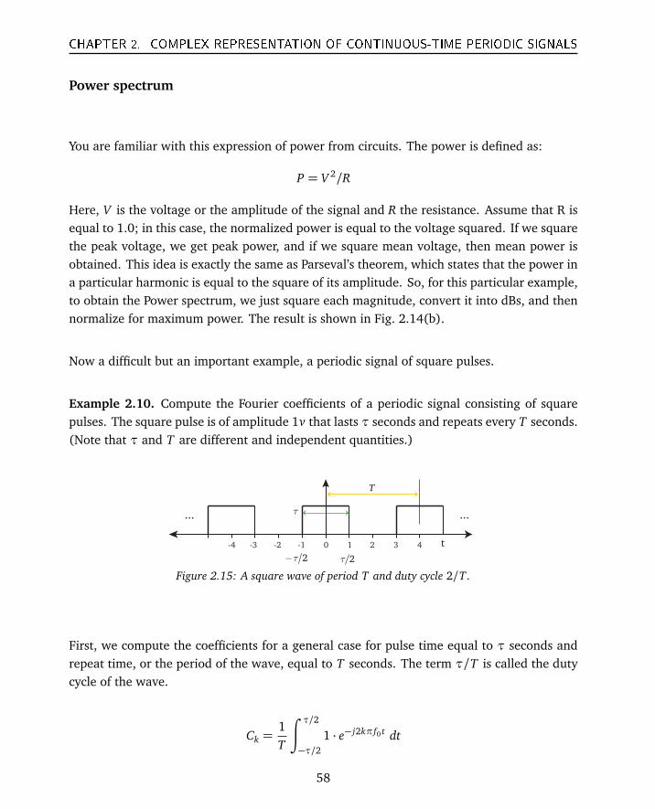
CHAPTER 2. COMPLEX REPRESENTATION OF CONTINUOUS-TIME PERIODIC SIGNALS
Power spectrum
You are familiar with this expression of power from circuits. The power is defined as:
P = V 2/R
Here, V is the voltage or the amplitude of the signal and R the resistance. Assume that R isequal to 1.0; in this case, the normalized power is equal to the voltage squared. If we squarethe peak voltage, we get peak power, and if we square mean voltage, then mean power isobtained. This idea is exactly the same as Parseval’s theorem, which states that the power ina particular harmonic is equal to the square of its amplitude. So, for this particular example,to obtain the Power spectrum, we just square each magnitude, convert it into dBs, and thennormalize for maximum power. The result is shown in Fig. 2.14(b).
Now a difficult but an important example, a periodic signal of square pulses.
Example 2.10. Compute the Fourier coefficients of a periodic signal consisting of squarepulses. The square pulse is of amplitude 1v that lasts τ seconds and repeats every T seconds.(Note that τ and T are different and independent quantities.)
t0 1 2 3 4 -4 -3 -2 -1
2τ2τ−
τ
T
Figure 2.15: A square wave of period T and duty cycle 2/T.
First, we compute the coefficients for a general case for pulse time equal to τ seconds andrepeat time, or the period of the wave, equal to T seconds. The term τ/T is called the dutycycle of the wave.
Ck =1T
∫ τ/2
−τ/21 · e− j2kπ f0 t dt
58

CHAPTER 2. COMPLEX REPRESENTATION OF CONTINUOUS-TIME PERIODIC SIGNALS
Note that outside of −τ/2< t < τ/2, the function is zero. This integral is given by
Ck =1T
e−( j2πk/T )t
− j2πk/T
τ/2
−τ/2
=1T
e( j2πk/T ) τ2 − e(− j2πk/T ) τ2
j2
1πk/T
=τ
Tsin(kπτ/T )
kπ(τ/T )
Replacing the duty cycle term τ with term r, the equation becomes easier to understand.
Ck = rsin(kπr)
kπr= rsinc(kπr).
Let us set the duty cycle of this signal to 0.5.
r =τ
T=
12
Substituting r in the above equation, we can write the expression for the coefficients of thissignal as:
Ck =12
sinc(kπ/2) (2.32)
This is the sinc function. It comes up so often in signal processing that it is probably thesecond most important equation in DSP after the Euler’s equation.
Now, we can plot the coefficients of the repeating continuous-time square pulse coefficientsfor various duty cycles. Note how the peakedness of the main lobe changes inversely with theduty cycle. A narrow pulse relative to the period in Fig. 2.16(a), has a shallower frequencyresponse than one that takes up more of the period. The zero crossings occur at inverse ofthe duty cycle. For r = 0.5, the zero crossing occurs at k = 2, for r = 0.25, the crossing is atk = 4, and for r = 0.75, the crossing occurs at n = 1.33. At r = 1.0, the pulse would be aflat line and it will have an impulse as its frequency response. For very small r, the pulse isdelta function-like and the response will go to a flat line. Note the usage of words, frequencyresponse. This is just another name for the spectrum.
Although the equation for this function is fairly easy, it takes a little while to develop intuitivefeeling. We cannot overemphasize the importance of this signal and you ought to spend sometime playing around with the parameters to understand the effect. We will of course keepcoming back to it in the next few chapters.
59
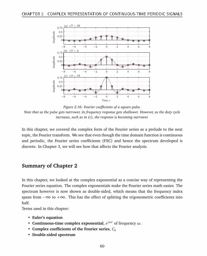
CHAPTER 2. COMPLEX REPRESENTATION OF CONTINUOUS-TIME PERIODIC SIGNALS
−8 −6 −4 −2 0 2 4 6 8
0
0.25
0.5
0.75(a)
Am
pli
tud
e
−8 −6 −4 −2 0 2 4 6 8
0
0.25
0.5
0.75(b)
Am
pli
tud
e
−8 −6 −4 −2 0 2 4 6 8
0
0.25
0.5
0.75(c)
Am
pli
tud
e
.25Tτ =
.5Tτ =
.75Tτ =
Time, t
Figure 2.16: Fourier coefficients of a square pulse.Note that as the pulse gets narrower, its frequency response gets shallower. However, as the duty cycle
increases, such as in (c), the response is becoming narrower.
In this chapter, we covered the complex form of the Fourier series as a prelude to the nexttopic, the Fourier transform. We see that even though the time domain function is continuousand periodic, the Fourier series coefficients (FSC) and hence the spectrum developed isdiscrete. In Chapter 3, we will see how that affects the Fourier analysis.
Summary of Chapter 2
In this chapter, we looked at the complex exponential as a concise way of representing theFourier series equation. The complex exponentials make the Fourier series math easier. Thespectrum however is now shown as double-sided, which means that the frequency indexspans from −∞ to +∞. This has the effect of splitting the trigonometric coefficients intohalf.Terms used in this chapter:
• Euler’s equation• Continuous-time complex exponential, e jωt of frequency ω.• Complex coefficients of the Fourier series, Ck
• Double-sided spectrum
60
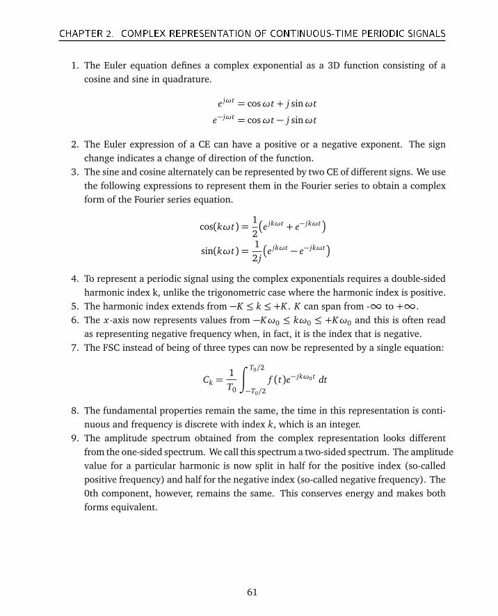
CHAPTER 2. COMPLEX REPRESENTATION OF CONTINUOUS-TIME PERIODIC SIGNALS
1. The Euler equation defines a complex exponential as a 3D function consisting of acosine and sine in quadrature.
e jωt = cosωt + j sinωt
e− jωt = cosωt − j sinωt
2. The Euler expression of a CE can have a positive or a negative exponent. The signchange indicates a change of direction of the function.
3. The sine and cosine alternately can be represented by two CE of different signs. We usethe following expressions to represent them in the Fourier series to obtain a complexform of the Fourier series equation.
cos(kωt) =12
e jkωt + e− jkωt
sin(kωt) =12 j
e jkωt − e− jkωt
4. To represent a periodic signal using the complex exponentials requires a double-sidedharmonic index k, unlike the trigonometric case where the harmonic index is positive.
5. The harmonic index extends from −K ≤ k ≤ +K . K can span from -∞ to +∞.6. The x-axis now represents values from −Kω0 ≤ kω0 ≤ +Kω0 and this is often read
as representing negative frequency when, in fact, it is the index that is negative.7. The FSC instead of being of three types can now be represented by a single equation:
Ck =1T0
∫ T0/2
−T0/2
f (t)e− jkω0 t dt
8. The fundamental properties remain the same, the time in this representation is conti-nuous and frequency is discrete with index k, which is an integer.
9. The amplitude spectrum obtained from the complex representation looks differentfrom the one-sided spectrum. We call this spectrum a two-sided spectrum. The amplitudevalue for a particular harmonic is now split in half for the positive index (so-calledpositive frequency) and half for the negative index (so-called negative frequency). The0th component, however, remains the same. This conserves energy and makes bothforms equivalent.
61
CHAPTER 2. COMPLEX REPRESENTATION OF CONTINUOUS-TIME PERIODIC SIGNALS
Questions
1. What is a complex exponential?2. What is the expression for a sine in the complex form?3. If we look along this axis, the CE appears as a circle. What axis is that? Which
parameter is not visible in this view?4. What is the value of e− jπ, e j2π, and e− j 3
4π.5. Why is this equation true? e jπ + 1= 06. What is the difference between two complex exponential of the same exponent but
different signs, such as e jωk t and e− jωk t . If we add these two signals, what do we getin the complex domain?
7. What dimensional space is required to plot a complex exponential?8. The term phasor is often used in relation to complex exponentials, what is it?9. If you plot a sinusoid plus its shifted version, sin(2ωt) + sin(2ωt + φ0), what is the
phase of the new signal?10. Represent this sinusoid as a complex exponential: cos
ωt + π4
.11. What is the relationship of the Taylor series to a sinusoid?12. What is the advantage of using complex exponential as a basis set instead of sines and
cosines?13. Given these CEs, give their expression in the Euler form: e− j3, (e− j4+ e− j2), and e− j π2 t .14. How would you express phase in the complex exponential form?15. Write the CE form of these signals:
(a) sin(7πt + π4 )
(b) cos(7πt + π4 )− sin(7πt − π
4 )(c) cos(3πt + π
2 )16. What is the magnitude of this complex signal, e−5 j t?17. The real part of a CE has a peak amplitude of 1 and the imaginary part has the peak
amplitude of 2. What is the peak and the average power of this signal?18. How do we transmit a complex signal? What does it look like?19. What does division by j mean?20. What does multiplication by j mean?21. What is the magnitude and phase of these signals:
(a)
sin(ωt)− cos(ωt)
(b)1
2 cos(ωt)− sin(ωt)
(c)
2cos(ωt)− 12 sin(ωt)
22. What is a single-sided spectrum? What does it represent?23. Given the amplitude spectrum, how would you compute the power spectrum?
62

CHAPTER 2. COMPLEX REPRESENTATION OF CONTINUOUS-TIME PERIODIC SIGNALS
24. What is two-sided spectrum of these signals?(a) f (t) = − cos(2πt) + cos(9πt) + sin(12πt)(b) f (t) = 2 cos(9πt) + 2 cos(18πt)
25. When plotting a two-sided spectrum, what does the x axis represent?26. If you are given the real and imaginary components of a signal, how do you compute
the phase? Is phase changing with time or frequency?27. For a complex signal, both real and imaginary signals can have nonzero phase, so what
is the phase of a complex signal? How is it different from the phases of the components?28. What is the relationship of the trigonometric coefficients to the complex coefficients?29. How do explain the idea of negative frequency?30. Why the spectrum of a complex signal is always one-sided?31. What is the mean and the peak power of a sinusoid of amplitude 1.0?32. If we have a periodic signal of square pulses with a duty cycle of 0.1. How much wider
is its spectrum as compared to a pulse that has a duty cycle of 0.5?33. What happens to the magnitude spectrum if phase of the signal changes?
63
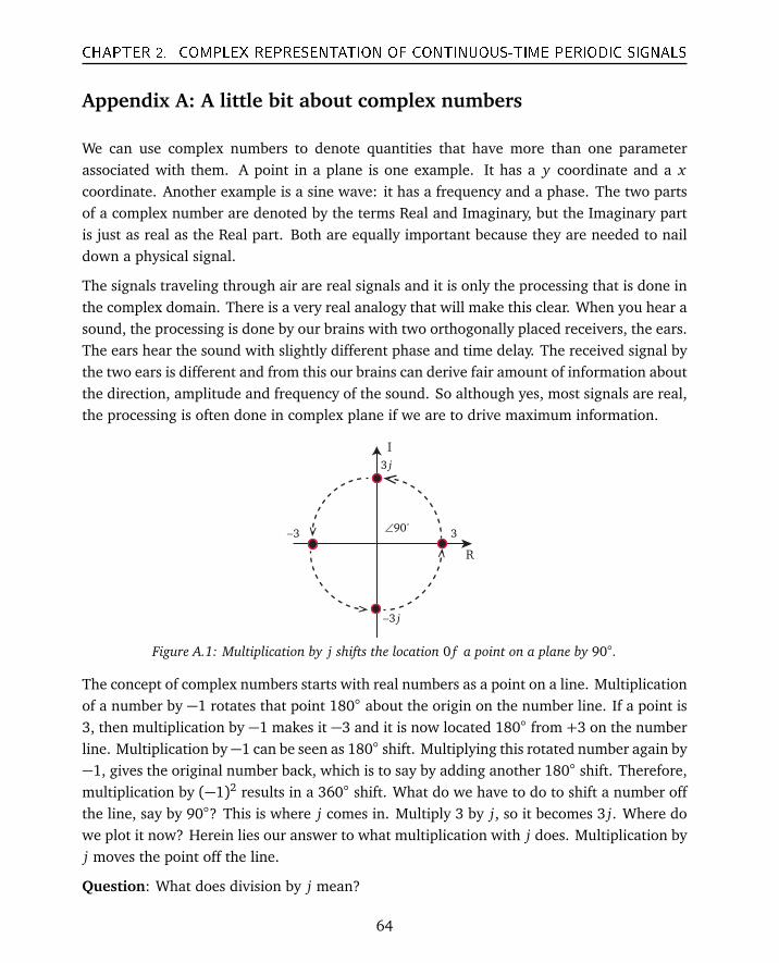
CHAPTER 2. COMPLEX REPRESENTATION OF CONTINUOUS-TIME PERIODIC SIGNALS
Appendix A: A little bit about complex numbers
We can use complex numbers to denote quantities that have more than one parameterassociated with them. A point in a plane is one example. It has a y coordinate and a xcoordinate. Another example is a sine wave: it has a frequency and a phase. The two partsof a complex number are denoted by the terms Real and Imaginary, but the Imaginary partis just as real as the Real part. Both are equally important because they are needed to naildown a physical signal.
The signals traveling through air are real signals and it is only the processing that is done inthe complex domain. There is a very real analogy that will make this clear. When you hear asound, the processing is done by our brains with two orthogonally placed receivers, the ears.The ears hear the sound with slightly different phase and time delay. The received signal bythe two ears is different and from this our brains can derive fair amount of information aboutthe direction, amplitude and frequency of the sound. So although yes, most signals are real,the processing is often done in complex plane if we are to drive maximum information.
90∠o
3
3 j
3 j−
3−
R
I
Figure A.1: Multiplication by j shifts the location 0 f a point on a plane by 90.
The concept of complex numbers starts with real numbers as a point on a line. Multiplicationof a number by −1 rotates that point 180 about the origin on the number line. If a point is3, then multiplication by −1 makes it −3 and it is now located 180 from +3 on the numberline. Multiplication by−1 can be seen as 180 shift. Multiplying this rotated number again by−1, gives the original number back, which is to say by adding another 180 shift. Therefore,multiplication by (−1)2 results in a 360 shift. What do we have to do to shift a number offthe line, say by 90? This is where j comes in. Multiply 3 by j, so it becomes 3 j. Where dowe plot it now? Herein lies our answer to what multiplication with j does. Multiplication byj moves the point off the line.
Question: What does division by j mean?
64
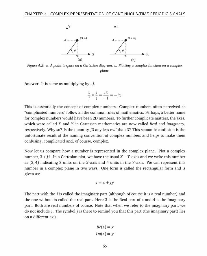
CHAPTER 2. COMPLEX REPRESENTATION OF CONTINUOUS-TIME PERIODIC SIGNALS
3
4
X
Y
(3,4)
3
4
R
I
3 4 j+
θ θ
(a) (b)
Figure A.2: a. A point is space on a Cartesian diagram. b. Plotting a complex function on a complexplane.
Answer: It is same as multiplying by – j.
xj×
jj=
j x−1= − j x .
This is essentially the concept of complex numbers. Complex numbers often perceived as“complicated numbers” follow all the common rules of mathematics. Perhaps, a better namefor complex numbers would have been 2D numbers. To further complicate matters, the axes,which were called X and Y in Cartesian mathematics are now called Real and Imaginary,respectively. Why so? Is the quantity j3 any less real than 3? This semantic confusion is theunfortunate result of the naming convention of complex numbers and helps to make themconfusing, complicated and, of course, complex.
Now let us compare how a number is represented in the complex plane. Plot a complexnumber, 3+ j4. In a Cartesian plot, we have the usual X − Y axes and we write this numberas (3,4) indicating 3 units on the X -axis and 4 units in the Y -axis. We can represent thisnumber in a complex plane in two ways. One form is called the rectangular form and isgiven as:
z = x + j y
The part with the j is called the imaginary part (although of course it is a real number) andthe one without is called the real part. Here 3 is the Real part of z and 4 is the Imaginarypart. Both are real numbers of course. Note that when we refer to the imaginary part, wedo not include j. The symbol j is there to remind you that this part (the imaginary part) lieson a different axis.
Re(z) = x
Im(z) = y
65
CHAPTER 2. COMPLEX REPRESENTATION OF CONTINUOUS-TIME PERIODIC SIGNALS
Alternate form of a complex number is the polar form.
z = M∠θ
where M is the magnitude and θ its angle with the real axis. The polar form that looks likea vector and in essence it is, is called a Phasor in signal processing. This idea comes fromcircuit analysis and is very useful in that realm. We also use it in signal processing but itseems to cause some conceptual difficulty. Mainly because, unlike in circuit analysis, in signalprocessing time is important. We are interested in signals in time domain and the phasor,which is a time-independent concept, is confusing. The phase as the term is used in signalprocessing is kind of the initial value of phase, where it is an angle in vector terminology.Question: If z = Ae jωt then what is its rectangular form? Answer: z = Acosωt + jAsinωt.We just substituted the Euler’s equation for the complex exponential e jωt . Think of e jωt as ashorthand functional notation for the expression cosωt + j sinωt. The real and imaginaryparts of z are given by
Re(z) = Acosωt
Im(z) = Asinωt.
Converting forms
1. Given a rectangular form z = x + j y then its polar form is equal to
M∠θ =
(
p
x2 + y2∠ tan−1 yx if x ≥ 0
p
x2 + y2∠
tan−1 yx +π
if x < 0
2. Given a polar form M∠θ then its rectangular form is given by
x + j y = M cosθ + jM sinθ
Example 2.11. Convert z = 5∠0.927 to rectangular form
Re(z) = 5cos(0.927) = 3
Im(z) = 5sin(0.927) = 4
⇒ z = 3+ j4
66
CHAPTER 2. COMPLEX REPRESENTATION OF CONTINUOUS-TIME PERIODIC SIGNALS
Example 2.12. Convert z = −1− j to polar form
M =Æ
(−1)2 + (−1)2 =p
2
θ = arctanyx+π, since x < 0
= arctan−1−1+π=
34π
⇒ z =p
2∠34π.
Example 2.13. Convert z = 1+ j to polar form.
M =Æ
(1)2 + (1)2 =p
2
θ = arctanyx
, since x > 0
= arctan11=
14π
⇒ z =p
2∠π/4.
Adding and Multiplying
Add in rectangular form, multiply in polar. Its easier this way.
1. Given z1 = a+ j b and z2 = c + jd then z1 + z2 = (a+ c) + j(b+ d).2. Given z1 = M1∠θ1 and z2 = M2∠θ2, then z1 · z2 = M1M2∠(θ1 + θ2).
Example 2.14. Add z2 =p
2∠0.785 and z2 = 5∠0.927.
Convert both to rectangular form.
z1 = 1+ j and z2 = 3+ j4
⇒ z3 = (1+ 3) + j(1+ 4) = 4+ j5.
Example 2.15. Multiply z1 = 1+ j and z2 = 3+ j4.
First convert to polar form and then multiply. Although multiplying these two complexnumbers in rectangular format looks easy, in general that is not the case. Polar form isbetter for multiplication and division.
z1 · z2 =p
2∠0.785× 5∠0.927= 5p
2∠1.71
67
CHAPTER 2. COMPLEX REPRESENTATION OF CONTINUOUS-TIME PERIODIC SIGNALS
Example 2.16. Divide z1 = 1+ j and z2 = 3+ j4.
z1
z2=p
2∠0.7855∠.927
=5p
2∠0.142
Conjugation
The conjugate for a complex number z, is given by z∗ = x − j y . For a complex exponentiale jωt is the complex conjugate of e− jωt . In polar format, the complex conjugate is same phasorbut rotating in the opposite direction.
Rule: If z = M∠θ , then z∗ = M∠− θ .
Useful properties of complex conjugates
|z|2 = zz∗
This relationship is used to compute the power of the signal. The magnitude of the signal canbe computed by half the sum of the signal and its complex conjugate. Note, the imaginarypart cancels out in this sum.
|z|=12
z + z∗
.
68
Chapter 3
Discrete-Time Signals andFourier Series Representation
Peter Gustav Lejeune Dirichlet1805 – 1859
Johann Peter Gustav Lejeune Dirichlet was a German mathematician who made deep contribu-tions to number theory, and to the theory of Fourier series and other topics in mathematicalanalysis; he is credited with being one of the first mathematicians to give the modern formaldefinition of a function. In 1829, Dirichlet published a famous memoir giving the conditions,showing for which functions the convergence of the Fourier series holds. Before Dirichlet’s solu-tion, not only Fourier, but also Poisson and Cauchy had tried unsuccessfully to find a rigorousproof of convergence. The memoir introduced Dirichlet’s test for the convergence of series. It alsointroduced the Dirichlet function as an example that not any function is integrable (the definiteintegral was still a developing topic at the time) and, in the proof of the theorem for the Fourierseries, it introduced the Dirichlet kernel and the Dirichlet integral. – From Wikipedia
69
CHAPTER 3. DISCRETE-TIME SIGNALS AND FOURIER SERIES REPRESENTATION
Fourier Series and Discrete-time Signals
In the previous two chapters, we discussed the Fourier series as applied to CT signals. Wesaw that the Fourier series can be used to create a representation of any periodic signal. Thisrepresentation is made using the sine and cosine functions or with complex exponentials.Both forms are equivalent. In the previous two chapters, the discussion was limited tocontinuous time (CT) signals. In this chapter we will discuss Fourier series analysis as appliedto discrete time (DT) signals.
Discrete signals are different
Although some data are naturally discrete such, as stock prices, number of students in a class,etc., many electronic signals we work with are sampled from analog signals, for example,voice, music, and medical/biological signals. The discrete signals are generated from analogsignals by a process called sampling. This is also known as Analog-to-Digital conversion.The generation of a discrete signal from an analog signal is done by an instantaneous measure-ment of the analog signal amplitude at uniform intervals.
Discrete vs. digital
In general terms, a discrete signal is continuous in amplitude but is discrete in time. Thismeans that it can have any value whatsoever for its amplitude but is defined or measuredonly at uniform time intervals. Hence, the term discrete applies to the time dimension andnot to the amplitude. For purposes of the Fourier analysis, we assume that the sampling isdone at uniform time intervals among the samples.
A discrete signal is often confused with the term digital signal. Although in common languagethey are thought of as the same thing, a digital signal is a special type of discrete signal. Likeany discrete signal, it is defined only at specific time intervals, but its amplitude is constrainedto specific values. There are binary digital signals where the amplitude is limited to only twovalues, +1,−1 or 0,1. A M -level signal can take on just one of 2M preset amplitudesonly. Hence, a digital signal is a specific type of discrete signal with constrained amplitudes.In this chapter, we will be discussing general discrete signals that include digital signals. Bothof these types of signals are called discrete time (DT) signals. We call the time of a samplingevent, the sampling instant. How fast or slow a signal is sampled is specified in terms of itssampling frequency, which is given in terms of the number of samples per second captured.
70
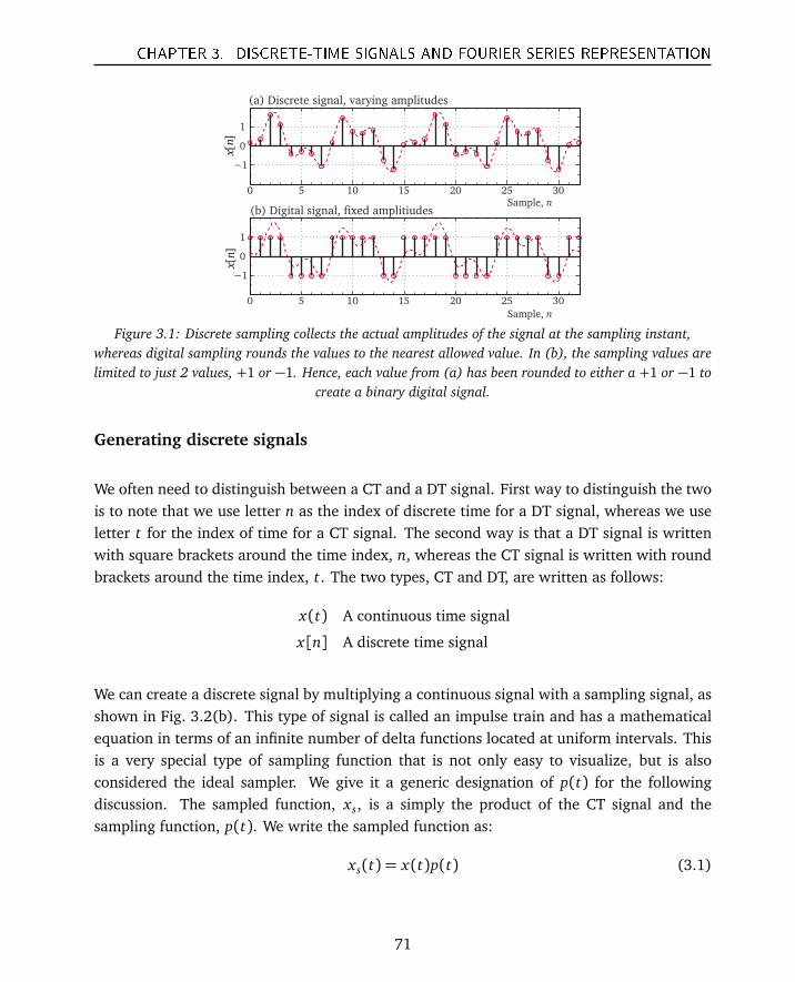
CHAPTER 3. DISCRETE-TIME SIGNALS AND FOURIER SERIES REPRESENTATION
0 5 10 15 20 25 30
−1
0
1
0 5 10 15 20 25 30
−1
0
1
(a) Discrete signal, varying amplitudes
(b) Digital signal, fixed amplitiudes
Sample, n
Sample, n
[]
xn
[]
xn
Figure 3.1: Discrete sampling collects the actual amplitudes of the signal at the sampling instant,whereas digital sampling rounds the values to the nearest allowed value. In (b), the sampling values arelimited to just 2 values, +1 or −1. Hence, each value from (a) has been rounded to either a +1 or −1 to
create a binary digital signal.
Generating discrete signals
We often need to distinguish between a CT and a DT signal. First way to distinguish the twois to note that we use letter n as the index of discrete time for a DT signal, whereas we useletter t for the index of time for a CT signal. The second way is that a DT signal is writtenwith square brackets around the time index, n, whereas the CT signal is written with roundbrackets around the time index, t. The two types, CT and DT, are written as follows:
x(t) A continuous time signal
x[n] A discrete time signal
We can create a discrete signal by multiplying a continuous signal with a sampling signal, asshown in Fig. 3.2(b). This type of signal is called an impulse train and has a mathematicalequation in terms of an infinite number of delta functions located at uniform intervals. Thisis a very special type of sampling function that is not only easy to visualize, but is alsoconsidered the ideal sampler. We give it a generic designation of p(t) for the followingdiscussion. The sampled function, xs, is a simply the product of the CT signal and thesampling function, p(t). We write the sampled function as:
xs(t) = x(t)p(t) (3.1)
71

CHAPTER 3. DISCRETE-TIME SIGNALS AND FOURIER SERIES REPRESENTATION
−5 −4 −3 −2 −1 0 1 2 3 4 5−1
0
1
0
1
−5 −4 −3 −2 −1 0 1 2 3 4 5−1
0
1
(a) A continuous-time signal
(b) An impluse train for sampling
−5 −4 −3 −2 −1 0 1 2 3 4 5
(c) Sampled signal
Time, t
Sample number, n
Sample number, n
()
xt
[]
nδ
[]
xn
sT
Figure 3.2: A CT signal sampled at uniform intervals Ts with an ideal sampling function. The discretesignal in (c) x[n] consists only of the discrete samples and nothing else. The continuous signal is shown
in dashed line for reference only. The receiver has no idea what it is. All it sees are the samples.
Sampling and Interpolation
Ideal sampling
Let us assume we have an impulse train, p(t) with period Ts as the sampling function.Multiplying this signal with the CT signal, as shown in Eq. (3.1), we get a continuous signalwith nonzero samples at the sample instants, referred to as nTs or n/Fs. Hence, the absolutetime is the sample number times the time in between each sample.
The sample time Ts is an independent parameter. The inverse of the sampling time, Ts, iscalled the sampling frequency, Fs, given in samples per second. For a signal sampled withthe ideal sampling function, an impulse train, the sampled signal is written per Eq. (3.1) as:
p(t) =∞∑
n=−∞δ(t − nTs)
xs(t) = x(t)∞∑
n=−∞δ(t − nTs) (3.2)
72
CHAPTER 3. DISCRETE-TIME SIGNALS AND FOURIER SERIES REPRESENTATION
The expression for a discrete signal of a sampled version of the CT signal is written as:
x[n] = xs(t)|t=nTs= x(nTs) (3.3)
The term x(nTs) with round brackets is continuous, as it is just the value of the CT signal attime nTs. The term x[n], however, is discrete because the index n is an integer by definition.The discrete signal x[n] has values only at points t = nTs where n is the integer samplenumber. It is undefined at all non-integers unlike the CT signal. The sampling time Ts relativeto the signal frequency determines how coarse or fine the sampling is. The discrete signalcan of course be real or complex. The individual value x[n] is called the nth sample of thesequence.
If we are given a CT signal of frequency f0, and this is being sampled at M samples persecond, we would compute the discrete signal from the continuous signal with this Matlabcode. Here, time t has been replaced with n/Fs.
1 xc = sin(2*pi*f0*t)2 Fs = 243 n = -48: 474 xd = sin(2*pi*n/Fs)
Reconstruction of an analog signal from discrete samples
Why sample signals? The signals are sampled for one big reason, to reduce their band-width. The other benefit from sampling is that signal processing on digital signals is “easier.”However, once sampled, processed, and transmitted, this signal must often then be convertedback to its analog form. The process of reconstructing a signal from discrete samples is calledinterpolation. This is the same idea as plotting a function. We compute a few values at someselected points and then connect those points to plot the continuous representation of thefunction. The reconstruction by machines, however, is not as straightforward and requiresgiving them an algorithm that they are able to do. This is where the subject gets complicated.
First, we note that there are two conditions for ideal reconstruction. One is that the signalmust have been ideally sampled to start with, i.e., by an impulse train such that the sampledvalues represent true amplitudes of a signal. Ideal sampling is hard to achieve but fortextbook purposes, we assume it can be done. In reality, lack of ideal sampling introducesdistortions.
73
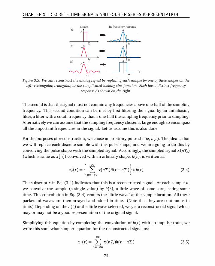
CHAPTER 3. DISCRETE-TIME SIGNALS AND FOURIER SERIES REPRESENTATION
sT
(a)
(b)
(c)
sT
A
A
A
W
W
W
Shape Its frequency response
sT
Figure 3.3: We can reconstruct the analog signal by replacing each sample by one of these shapes on theleft: rectangular, triangular, or the complicated-looking sinc function. Each has a distinct frequency
response as shown on the right.
The second is that the signal must not contain any frequencies above one-half of the samplingfrequency. This second condition can be met by first filtering the signal by an antialiasingfilter, a filter with a cutoff frequency that is one-half the sampling frequency prior to sampling.Alternatively we can assume that the sampling frequency chosen is large enough to encompassall the important frequencies in the signal. Let us assume this is also done.
For the purposes of reconstruction, we chose an arbitrary pulse shape, h(t). The idea is thatwe will replace each discrete sample with this pulse shape, and we are going to do this byconvolving the pulse shape with the sampled signal. Accordingly, the sampled signal x(nTs)(which is same as x[n]) convolved with an arbitrary shape, h(t), is written as:
xr(t) =
∞∑
n=−∞x(nTs)δ(t − nTs)
∗ h(t) (3.4)
The subscript r in Eq. (3.4) indicates that this is a reconstructed signal. At each sample n,we convolve the sample (a single value) by h(t), a little wave of some sort, lasting sometime. This convolution in Eq. (3.4) centers the “little wave” at the sample location. All thesepackets of waves are then arrayed and added in time. (Note that they are continuous intime.) Depending on the h(t) or the little wave selected, we get a reconstructed signal whichmay or may not be a good representation of the original signal.
Simplifying this equation by completing the convolution of h(t) with an impulse train, wewrite this somewhat simpler equation for the reconstructed signal as:
xr(t) =∞∑
n=−∞x(nTs)h(t − nTs) (3.5)
74
CHAPTER 3. DISCRETE-TIME SIGNALS AND FOURIER SERIES REPRESENTATION
To examine the possibilities for shapes, h(t), following three options are picked; a rectangularpulse, a triangular pulse, and a sinc function. It turns out that these three pretty much covermost of what is used in practice. Each of these “shapes” has a distinctive frequency responseas shown in Fig. 3.3. The frequency response is used to determine the effect these shapes willhave on the reconstructed signal. Of course, we have not yet fully explained what a frequencyresponse is. A frequency response is meant to identify or characterize physical systems. It isdone by injecting an impulse into a system and then noting the output. This output is calledthe frequency response of the system. It is often characterized by the magnitude of theresponse, and the phase, so it is very similar to the idea of a spectrum. In industry these twoterms are used interchangeably.
The sampled signals often require that we reconvert them back to their analog form. Wediscuss three main ways this is done. Intuitively speaking, the process consists of replacingeach sample with a little wave.
Method 1: Zero-Order-Hold
Figure 3.3(a) shows a single square pulse. The idea is to replace each sample with a squarepulse of amplitude equal to the sample value. This basically means that the sample amplitudeis held to the next sampling instant in a flat line. The hold time period is Ts. This formof reconstruction is called sample-and-hold or zero-order-hold (ZOH) method of signalreconstruction. Zero in ZOH is the slope of this interpolation function, a straight line ofzero slope connecting one sample to the next. It is a simplistic method but if done withsmall enough resolution, that is a very narrow rectangle in time, ZOH can do a decent job ofreconstructing the signal. The shape function h(t) in this case is a rectangle.
h(t) = rect(t − nTs) (3.6)
The reconstructed signal is now given using the general expression of Eq. (3.4), where wesubstitute the [rect] shape into Eq. (3.5) to get:
xr(t) =∞∑
n=−∞x(nTs)rect(t − nTs) (3.7)
We show the index as going from −∞ < n < +∞ as the general form. In Fig. 3.4(a), wesee a signal reconstructed using a ZOH circuit, in which the rectangular pulse is scaled andrepeated at each sample.
75

CHAPTER 3. DISCRETE-TIME SIGNALS AND FOURIER SERIES REPRESENTATION
••
•
•
•
•
••
••
•
•
•
•
••
••
•
•
•
••
•
•
•
•
•
•
()
sx
nT
sT
•••••
•••••
Time,s
nT
(a) Signal and the samples
(b) Replacing each sample with a rectangle
()
xt
Figure 3.4: A zero-order-hold: hold each sample value to the next sample time.
(a) Signal and the samples
(b) Replacing each sample with a triangle
[]
xn
••
•
•
•
•
••
••
•
•
•
•
••
••
•
•
•
••
•
•
•
•
•
•
()
sx
nT
sT
•••••••••
•••••
Time,snT
Figure 3.5: A First-order-hold (FOH): replace each sample with a triangle of twice the time-width.
Method 2: First-Order-Hold (linear interpolation)
Zero-order hold gives us a stair-step like signal. Now, instead of a square pulse, we replaceeach sample with a triangle of width 2Ts as given by the expression
h(t) =
1− t/T 0< t < Ts
1+ t/T Ts < t < 2Ts
0 else
(3.8)
This function is shaped like a triangle and the reconstructed signal equation from Eq. (3.5)now becomes
xr(t) =∞∑
n=−∞x(nTs) tri
t − nTs
Ts
(3.9)
Figure 3.5(b) shows that instead of nonoverlapping rectangles as in ZOH, we use overlappingtriangles. This is because the width of the triangle is set to twice the sample time. Thisdouble-width does two things: it keeps the amplitude the same as the case of the rectangle
76
CHAPTER 3. DISCRETE-TIME SIGNALS AND FOURIER SERIES REPRESENTATION
and it fills the in-between points in a linear fashion. This method is also called a linearinterpolation as we are just connecting the points. This is also called the First-order-hold(FOH) because we are connecting the adjacent samples with a line of linear slope. Why youmay ask use triangles when we can just connect the samples? The answer to this query is thatmachines cannot “see” the samples nor “connect” the samples. Addition is about all they cando well. Hence, this method replaces the linear interpolation as you and I might do, visuallywith a simple addition of displaced triangles. It also gives us a hint as to how we can useany shape we want and in fact of any length, not just two times the sample time! Sinc pulseis such a shape.
Method 3: Sinc interpolation
We used triangles in FOH and that seems to produce a better-looking reconstructed signalthan ZOH. We can, in fact use just about any shape we want to represent a sample, fromthe rectangle to one composed of a complex shape, such as a sinc function. A sinc functionseems like an unlikely choice as it is noncausal (as it extends into the future) but it is infact anextension of the idea of the first two methods. Both ZOH and FOH are forms of polynomialcurve fit. The FOH is a linear polynomial, and we continue in this fashion with second-orderon up to infinite orders to represent just about any type of wiggly shape we can think of.A sinc function, an infinite order polynomial, is the basis of perfect reconstruction. Thereconstructed signal becomes a sum of scaled, shifted sinc functions same as was donewith triangular shapes. Even though the sinc function is an infinitely long function, it iszero-valued at regular intervals. This interval is equal to the sampling period. As each sincpulse lobe crosses zero at only the sampling instants, the summed signal where each sinc iscentered at a different time, adds no interference (quantity of its own amplitude) to othersinc pulses centered at other times. Hence, this shape is considered to be free of inter-symbolinterference (ISI).
The equation obtained for the reconstructed signal in this case is similar to the first two cases,with the reconstructed signal summed with each sinc located at nTs.
h(t) = sinc(t − nTs)
xr(t) =∞∑
n=−∞x(nTs) sinc(t − nTs)
(3.10)
Figure 3.6 shows the sinc reconstruction process for a signal with each sample being replacedby a sinc function and the resulting reconstructed signal compared to the original signal inFig. 3.6(b).
77
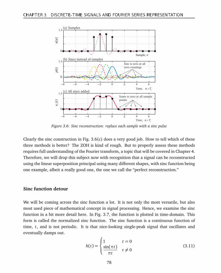
CHAPTER 3. DISCRETE-TIME SIGNALS AND FOURIER SERIES REPRESENTATION
0
1.5
−8 −6 −4 −2 0 2 4 6
0
1.5
−8 −6 −4 −2 0 2 4 6
0
1.5Sums to zero at all sample
points
Time,
Sinc is zero at all
zero crossings
(a) Samples
(b) Sincs instead of samples
(c) All sincs added
x[n]
(t)
px()
rt
Sample, n
sn T×
Time, s
n T×
Figure 3.6: Sinc reconstruction: replace each sample with a sinc pulse
Clearly the sinc construction in Fig. 3.6(c) does a very good job. How to tell which of thesethree methods is better? The ZOH is kind of rough. But to properly assess these methodsrequires full understanding of the Fourier transform, a topic that will be covered in Chapter 4.Therefore, we will drop this subject now with recognition that a signal can be reconstructedusing the linear superposition principal using many different shapes, with sinc function beingone example, albeit a really good one, the one we call the “perfect reconstruction.”
Sinc function detour
We will be coming across the sinc function a lot. It is not only the most versatile, but alsomost used piece of mathematical concept in signal processing. Hence, we examine the sincfunction in a bit more detail here. In Fig. 3.7, the function is plotted in time-domain. Thisform is called the normalized sinc function. The sinc function is a continuous function oftime, t, and is not periodic. It is that nice-looking single-peak signal that oscillates andeventually damps out.
h(t) =
1 t = 0sin(πt)πt
t 6= 0(3.11)
78
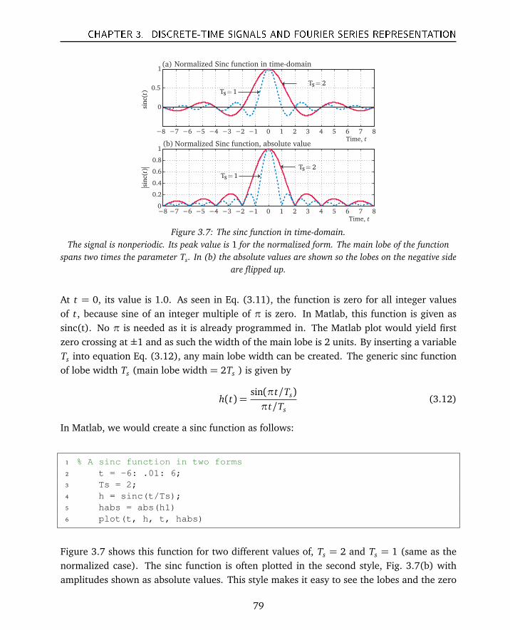
CHAPTER 3. DISCRETE-TIME SIGNALS AND FOURIER SERIES REPRESENTATION
−8 −7 −6 −5 −4 −3 −2 −1 0 1 2 3 4 5 6 7 8
0
0.5
1
−8 −7 −6 −5 −4 −3 −2 −1 0 1 2 3 4 5 6 7 80
0.2
0.4
0.6
0.8
1
(a) Normalized Sinc function in time-domain
1sT =
2sT =
1sT =
2sT =
Normalized Sinc function, absolute value(b)Time, t
Time, t
sin
c()
tsi
nc(
)t
Figure 3.7: The sinc function in time-domain.The signal is nonperiodic. Its peak value is 1 for the normalized form. The main lobe of the function
spans two times the parameter Ts. In (b) the absolute values are shown so the lobes on the negative sideare flipped up.
At t = 0, its value is 1.0. As seen in Eq. (3.11), the function is zero for all integer valuesof t, because sine of an integer multiple of π is zero. In Matlab, this function is given assinc(t). No π is needed as it is already programmed in. The Matlab plot would yield firstzero crossing at ±1 and as such the width of the main lobe is 2 units. By inserting a variableTs into equation Eq. (3.12), any main lobe width can be created. The generic sinc functionof lobe width Ts (main lobe width = 2Ts ) is given by
h(t) =sin(πt/Ts)πt/Ts
(3.12)
In Matlab, we would create a sinc function as follows:
1 % A sinc function in two forms2 t = -6: .01: 6;3 Ts = 2;4 h = sinc(t/Ts);5 habs = abs(h1)6 plot(t, h, t, habs)
Figure 3.7 shows this function for two different values of, Ts = 2 and Ts = 1 (same as thenormalized case). The sinc function is often plotted in the second style, Fig. 3.7(b) withamplitudes shown as absolute values. This style makes it easy to see the lobes and the zero
79
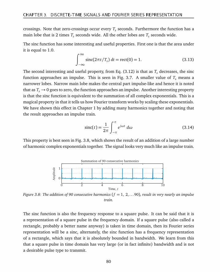
CHAPTER 3. DISCRETE-TIME SIGNALS AND FOURIER SERIES REPRESENTATION
crossings. Note that zero-crossings occur every Ts seconds. Furthermore the function has amain lobe that is 2 times Ts seconds wide. All the other lobes are Ts seconds wide.
The sinc function has some interesting and useful properties. First one is that the area underit is equal to 1.0.
∫ ∞
−∞sinc(2πt/Ts) dt= rect(0) = 1. (3.13)
The second interesting and useful property, from Eq. (3.12) is that as Ts decreases, the sincfunction approaches an impulse. This is seen in Fig. 3.7. A smaller value of Ts means anarrower lobes. Narrow main lobe makes the central part impulse-like and hence it is notedthat as Ts→ 0 goes to zero, the function approaches an impulse. Another interesting propertyis that the sinc function is equivalent to the summation of all complex exponentials. This is amagical property in that it tells us how Fourier transform works by scaling these exponentials.We have shown this effect in Chapter 1 by adding many harmonics together and noting thatthe result approaches an impulse train.
sinc(t) =1
2π
∫ π
−πe jωt dω (3.14)
This property is best seen in Fig. 3.8, which shows the result of an addition of a large numberof harmonic complex exponentials together. The signal looks very much like an impulse train.
0 2 4 6 8 10
0
1
Time, t
Am
pli
tud
e
Summation of 90 consecutive harmonics
Figure 3.8: The addition of 90 consecutive harmonics ( f = 1, 2, . . . 90), result in very nearly an impulsetrain.
The sinc function is also the frequency response to a square pulse. It can be said that it isa representation of a square pulse in the frequency domain. If a square pulse (also called arectangle, probably a better name anyway) is taken in time domain, then its Fourier seriesrepresentation will be a sinc, alternately, the sinc function has a frequency representationof a rectangle, which says that it is absolutely bounded in bandwidth. We learn from thisthat a square pulse in time domain has very large (or in fact infinite) bandwidth and is nota desirable pulse type to transmit.
80
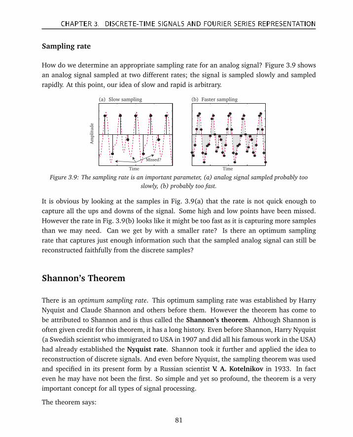
CHAPTER 3. DISCRETE-TIME SIGNALS AND FOURIER SERIES REPRESENTATION
Sampling rate
How do we determine an appropriate sampling rate for an analog signal? Figure 3.9 showsan analog signal sampled at two different rates; the signal is sampled slowly and sampledrapidly. At this point, our idea of slow and rapid is arbitrary.
Time
(a) Slow sampling
Time
(b) Faster sampling
Missed?
Am
pli
tud
e
Figure 3.9: The sampling rate is an important parameter, (a) analog signal sampled probably tooslowly, (b) probably too fast.
It is obvious by looking at the samples in Fig. 3.9(a) that the rate is not quick enough tocapture all the ups and downs of the signal. Some high and low points have been missed.However the rate in Fig. 3.9(b) looks like it might be too fast as it is capturing more samplesthan we may need. Can we get by with a smaller rate? Is there an optimum samplingrate that captures just enough information such that the sampled analog signal can still bereconstructed faithfully from the discrete samples?
Shannon’s Theorem
There is an optimum sampling rate. This optimum sampling rate was established by HarryNyquist and Claude Shannon and others before them. However the theorem has come tobe attributed to Shannon and is thus called the Shannon’s theorem. Although Shannon isoften given credit for this theorem, it has a long history. Even before Shannon, Harry Nyquist(a Swedish scientist who immigrated to USA in 1907 and did all his famous work in the USA)had already established the Nyquist rate. Shannon took it further and applied the idea toreconstruction of discrete signals. And even before Nyquist, the sampling theorem was usedand specified in its present form by a Russian scientist V. A. Kotelnikov in 1933. In facteven he may have not been the first. So simple and yet so profound, the theorem is a veryimportant concept for all types of signal processing.
The theorem says:
81
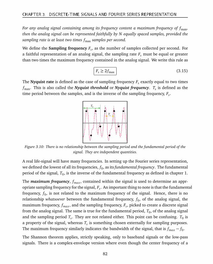
CHAPTER 3. DISCRETE-TIME SIGNALS AND FOURIER SERIES REPRESENTATION
For any analog signal containing among its frequency content a maximum frequency of fmax,then the analog signal can be represented faithfully by N equally spaced samples, provided thesampling rate is at least two times fmax samples per second.
We define the Sampling frequency Fs, as the number of samples collected per second. Fora faithful representation of an analog signal, the sampling rate Fs must be equal or greaterthan two times the maximum frequency contained in the analog signal. We write this rule as
Fs ≥ 2 fmax (3.15)
The Nyquist rate is defined as the case of sampling frequency Fs exactly equal to two timesfmax. This is also called the Nyquist threshold or Nyquist frequency. Ts is defined as thetime period between the samples, and is the inverse of the sampling frequency, Fs.
0T
sT
Figure 3.10: There is no relationship between the sampling period and the fundamental period of thesignal. They are independent quantities.
A real life-signal will have many frequencies. In setting up the Fourier series representation,we defined the lowest of all its frequencies, f0, as its fundamental frequency. The fundamentalperiod of the signal, T0, is the inverse of the fundamental frequency as defined in chapter 1.
The maximum frequency, fmax , contained within the signal is used to determine an appr-opriate sampling frequency for the signal, Fs. An important thing to note is that the fundamentalfrequency, f0, is not related to the maximum frequency of the signal. Hence, there is norelationship whatsoever between the fundamental frequency, f0, of the analog signal, themaximum frequency, fmax , and the sampling frequency, Fs, picked to create a discrete signalfrom the analog signal. The same is true for the fundamental period, T0, of the analog signaland the sampling period Ts. They are not related either. This point can be confusing. T0 isa property of the signal, whereas Ts is something chosen externally for sampling purposes.The maximum frequency similarly indicates the bandwidth of the signal, that is fmax − f0.
The Shannon theorem applies, strictly speaking, only to baseband signals or the low-passsignals. There is a complex-envelope version where even though the center frequency of a
82
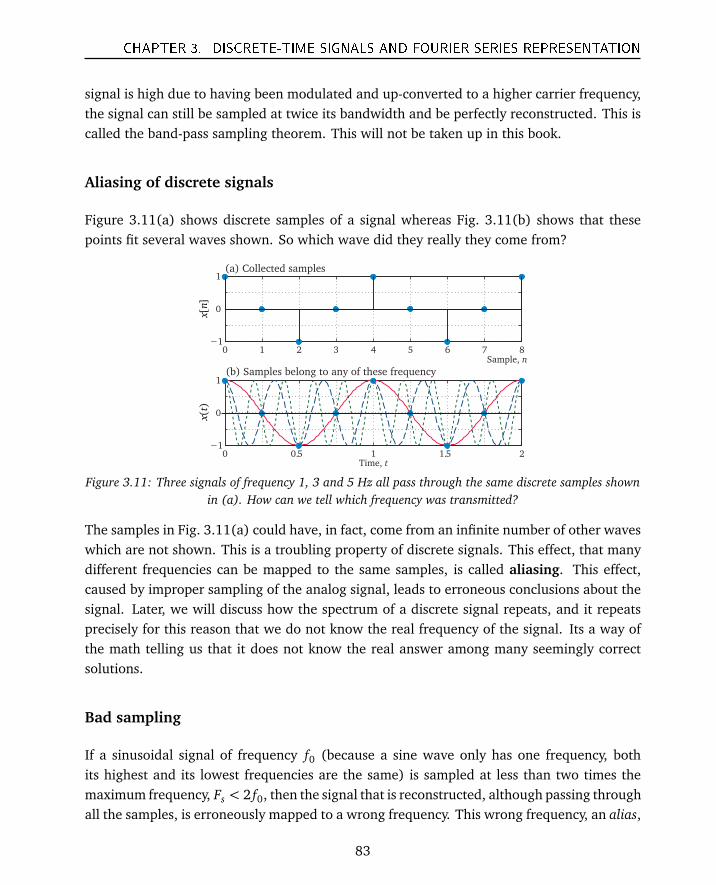
CHAPTER 3. DISCRETE-TIME SIGNALS AND FOURIER SERIES REPRESENTATION
signal is high due to having been modulated and up-converted to a higher carrier frequency,the signal can still be sampled at twice its bandwidth and be perfectly reconstructed. This iscalled the band-pass sampling theorem. This will not be taken up in this book.
Aliasing of discrete signals
Figure 3.11(a) shows discrete samples of a signal whereas Fig. 3.11(b) shows that thesepoints fit several waves shown. So which wave did they really they come from?
0 1 2 3 4 5 6 7 8−1
0
1
0 0.5 1 1.5 2−1
0
1
(a) Collected samples
(b) Samples belong to any of these frequencySample, n
Time, t
[]
xn
()
xt
Figure 3.11: Three signals of frequency 1, 3 and 5 Hz all pass through the same discrete samples shownin (a). How can we tell which frequency was transmitted?
The samples in Fig. 3.11(a) could have, in fact, come from an infinite number of other waveswhich are not shown. This is a troubling property of discrete signals. This effect, that manydifferent frequencies can be mapped to the same samples, is called aliasing. This effect,caused by improper sampling of the analog signal, leads to erroneous conclusions about thesignal. Later, we will discuss how the spectrum of a discrete signal repeats, and it repeatsprecisely for this reason that we do not know the real frequency of the signal. Its a way ofthe math telling us that it does not know the real answer among many seemingly correctsolutions.
Bad sampling
If a sinusoidal signal of frequency f0 (because a sine wave only has one frequency, bothits highest and its lowest frequencies are the same) is sampled at less than two times themaximum frequency, Fs < 2 f0, then the signal that is reconstructed, although passing throughall the samples, is erroneously mapped to a wrong frequency. This wrong frequency, an alias,
83
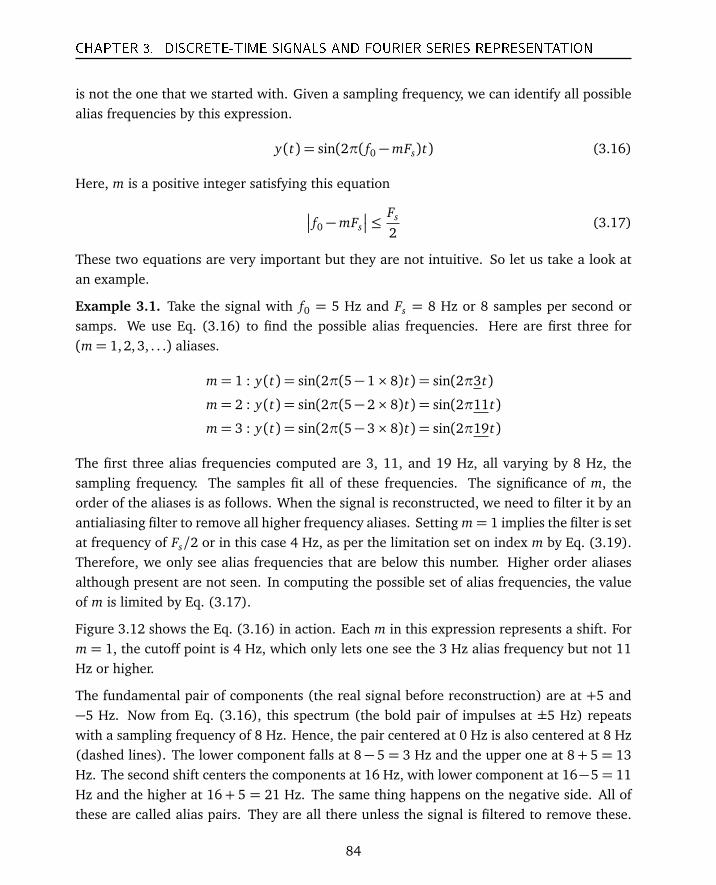
CHAPTER 3. DISCRETE-TIME SIGNALS AND FOURIER SERIES REPRESENTATION
is not the one that we started with. Given a sampling frequency, we can identify all possiblealias frequencies by this expression.
y(t) = sin(2π( f0 −mFs)t) (3.16)
Here, m is a positive integer satisfying this equation
f0 −mFs
≤Fs
2(3.17)
These two equations are very important but they are not intuitive. So let us take a look atan example.
Example 3.1. Take the signal with f0 = 5 Hz and Fs = 8 Hz or 8 samples per second orsamps. We use Eq. (3.16) to find the possible alias frequencies. Here are first three for(m= 1,2, 3, . . .) aliases.
m= 1 : y(t) = sin(2π(5− 1× 8)t) = sin(2π3t)
m= 2 : y(t) = sin(2π(5− 2× 8)t) = sin(2π11t)
m= 3 : y(t) = sin(2π(5− 3× 8)t) = sin(2π19t)
The first three alias frequencies computed are 3, 11, and 19 Hz, all varying by 8 Hz, thesampling frequency. The samples fit all of these frequencies. The significance of m, theorder of the aliases is as follows. When the signal is reconstructed, we need to filter it by anantialiasing filter to remove all higher frequency aliases. Setting m= 1 implies the filter is setat frequency of Fs/2 or in this case 4 Hz, as per the limitation set on index m by Eq. (3.19).Therefore, we only see alias frequencies that are below this number. Higher order aliasesalthough present are not seen. In computing the possible set of alias frequencies, the valueof m is limited by Eq. (3.17).
Figure 3.12 shows the Eq. (3.16) in action. Each m in this expression represents a shift. Form = 1, the cutoff point is 4 Hz, which only lets one see the 3 Hz alias frequency but not 11Hz or higher.
The fundamental pair of components (the real signal before reconstruction) are at +5 and−5 Hz. Now from Eq. (3.16), this spectrum (the bold pair of impulses at ±5 Hz) repeatswith a sampling frequency of 8 Hz. Hence, the pair centered at 0 Hz is also centered at 8 Hz(dashed lines). The lower component falls at 8− 5 = 3 Hz and the upper one at 8+ 5 = 13Hz. The second shift centers the components at 16 Hz, with lower component at 16−5= 11Hz and the higher at 16+ 5 = 21 Hz. The same thing happens on the negative side. All ofthese are called alias pairs. They are all there unless the signal is filtered to remove these.
84
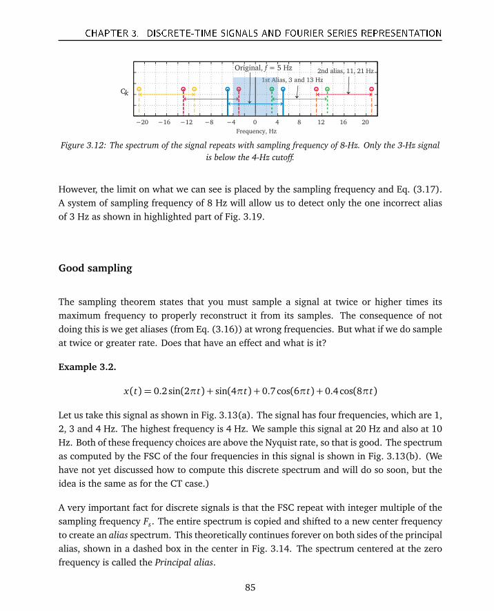
CHAPTER 3. DISCRETE-TIME SIGNALS AND FOURIER SERIES REPRESENTATION
−20 −16 −12 −8 −4 0 4 8 12 16 20
Original, f = 5 Hz
1st Alias, 3 and 13 Hz
2nd alias, 11, 21 Hz
Ck
Frequency, Hz
1st Alias, 3 and 13 Hz1st Alias, 3 and 13 Hz
Figure 3.12: The spectrum of the signal repeats with sampling frequency of 8-Hz. Only the 3-Hz signalis below the 4-Hz cutoff.
However, the limit on what we can see is placed by the sampling frequency and Eq. (3.17).A system of sampling frequency of 8 Hz will allow us to detect only the one incorrect aliasof 3 Hz as shown in highlighted part of Fig. 3.19.
Good sampling
The sampling theorem states that you must sample a signal at twice or higher times itsmaximum frequency to properly reconstruct it from its samples. The consequence of notdoing this is we get aliases (from Eq. (3.16)) at wrong frequencies. But what if we do sampleat twice or greater rate. Does that have an effect and what is it?
Example 3.2.
x(t) = 0.2 sin(2πt) + sin(4πt) + 0.7cos(6πt) + 0.4 cos(8πt)
Let us take this signal as shown in Fig. 3.13(a). The signal has four frequencies, which are 1,2, 3 and 4 Hz. The highest frequency is 4 Hz. We sample this signal at 20 Hz and also at 10Hz. Both of these frequency choices are above the Nyquist rate, so that is good. The spectrumas computed by the FSC of the four frequencies in this signal is shown in Fig. 3.13(b). (Wehave not yet discussed how to compute this discrete spectrum and will do so soon, but theidea is the same as for the CT case.)
A very important fact for discrete signals is that the FSC repeat with integer multiple of thesampling frequency Fs. The entire spectrum is copied and shifted to a new center frequencyto create an alias spectrum. This theoretically continues forever on both sides of the principalalias, shown in a dashed box in the center in Fig. 3.14. The spectrum centered at the zerofrequency is called the Principal alias.
85
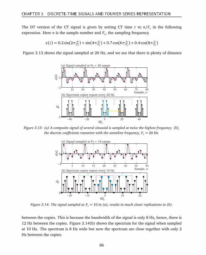
CHAPTER 3. DISCRETE-TIME SIGNALS AND FOURIER SERIES REPRESENTATION
The DT version of the CT signal is given by setting CT time t to n/Fs in the followingexpression. Here n is the sample number and Fs, the sampling frequency.
x(t) = 0.2 sin(2π nFs) + sin(4π n
Fs) + 0.7 cos(6π n
Fs) + 0.4 cos(8π n
Fs)
Figure 3.13 shows the signal sampled at 20 Hz, and we see that there is plenty of distance
10 20 30 40 50 60 70 80−2
0
−40 −20 0 20 400
skF
Sample, n
kC
(a) Signal sampled at Fs = 20 samps
(b) Spectrum copies repeat every 20 Hz
[]
xn
Figure 3.13: (a) A composite signal of several sinusoid is sampled at twice the highest frequency. (b),the discrete coefficients repeating with the sampling frequency, Fs = 20 Hz.
5 10 15 20 25 30 35 40−2
0
−20 −10 0 10 200
skF
Sample, n(b)
kC
[]
xn
Spectrum copies repeat every 10 Hz
(a) Signal sampled at Fs = 10 samps
Figure 3.14: The signal sampled at Fs = 10 in (a), results in much closer replications in (b).
between the copies. This is because the bandwidth of the signal is only 8 Hz, hence, there is12 Hz between the copies. Figure 3.14(b) shows the spectrum for the signal when sampledat 10 Hz. The spectrum is 8 Hz wide but now the spectrum are close together with only 2Hz between the copies.
86
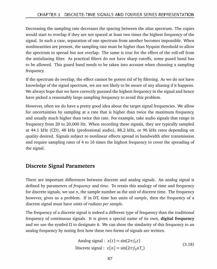
CHAPTER 3. DISCRETE-TIME SIGNALS AND FOURIER SERIES REPRESENTATION
Decreasing the sampling rate decreases the spacing between the alias spectrum. The copieswould start to overlap if they are not spaced at least two times the highest frequency of thesignal. In such a case, separation of one spectrum from another becomes impossible. Whennonlinearities are present, the sampling rate must be higher than Nyquist threshold to allowthe spectrum to spread but not overlap. The same is true for the effect of the roll-off fromthe antialiasing filter. As practical filters do not have sharp cutoffs, some guard band hasto be allowed. This guard band needs to be taken into account when choosing a samplingfrequency.
If the spectrum do overlap, the effect cannot be gotten rid of by filtering. As we do not haveknowledge of the signal spectrum, we are not likely to be aware of any aliasing if it happens.We always hope that we have correctly guessed the highest frequency in the signal and hencehave picked a reasonably large sampling frequency to avoid this problem.
However, often we do have a pretty good idea about the target signal frequencies. We allowfor uncertainties by sampling at a rate that is higher than twice the maximum frequency,and usually much higher than twice this rate. For example, take audio signals that range infrequency from 20 to 20,000 Hz. When recording these signals, they are typically sampledat 44.1 kHz (CD), 48 kHz (professional audio), 88.2 kHz, or 96 kHz rates depending onquality desired. Signals subject to nonlinear effects spread in bandwidth after transmissionand require sampling rates of 4 to 16 times the highest frequency to cover the spreading ofthe signal.
Discrete Signal Parameters
There are important differences between discrete and analog signals. An analog signal isdefined by parameters of frequency and time. To retain this analogy of time and frequencyfor discrete signals, we use n, the sample number as the unit of discrete time. The frequencyhowever, gives us a problem. If in DT, time has units of sample, then the frequency of adiscrete signal must have units of radians per sample.
The frequency of a discrete signal is indeed a different type of frequency than the traditionalfrequency of continuous signals. It is given a special name of its own, digital frequencyand we use the symbol Ω to designate it. We can show the similarity of this frequency to ananalog frequency by noting first how these two forms of signals are written.
Analog signal : x(t) = sin(2π f0 t)
Discrete signal : x[n] = sin(2π f0nTs)(3.18)
87
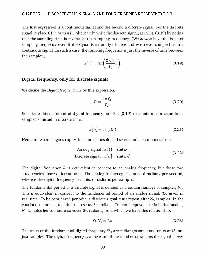
CHAPTER 3. DISCRETE-TIME SIGNALS AND FOURIER SERIES REPRESENTATION
The first expression is a continuous signal and the second a discrete signal. For the discretesignal, replace CT, t, with nTs. Alternately, write the discrete signal, as in Eq. (3.19) by notingthat the sampling time is inverse of the sampling frequency. (We always have the issue ofsampling frequency even if the signal is naturally discrete and was never sampled from acontinuous signal. In such a case, the sampling frequency is just the inverse of time betweenthe samples.)
x[n] = sin
2π f0Fs
n
. (3.19)
Digital frequency, only for discrete signals
We define the Digital frequency, Ω by this expression.
Ω=2π f0
Fs(3.20)
Substitute this definition of digital frequency into Eq. (3.19) to obtain a expression for asampled sinusoid in discrete time.
x[n] = sin(Ωn) (3.21)
Here are two analogous expressions for a sinusoid, a discrete and a continuous form.
Analog signal : x(t) = sin(ωt)
Discrete signal : x[n] = sin(Ωn)(3.22)
The digital frequency Ω is equivalent in concept to an analog frequency, but these two“frequencies” have different units. The analog frequency has units of radians per second,whereas the digital frequency has units of radians per sample.
The fundamental period of a discrete signal is defined as a certain number of samples, N0.This is equivalent in concept to the fundamental period of an analog signal, T0, given inreal time. To be considered periodic, a discrete signal must repeat after N0 samples. In thecontinuous domain, a period represents 2π radians. To retain equivalence in both domains,N0 samples hence must also cover 2π radians, from which we have this relationship.
Ω0N0 = 2π (3.23)
The units of the fundamental digital frequency Ω0 are radians/sample and units of N0 arejust samples. The digital frequency is a measure of the number of radians the signal moves
88
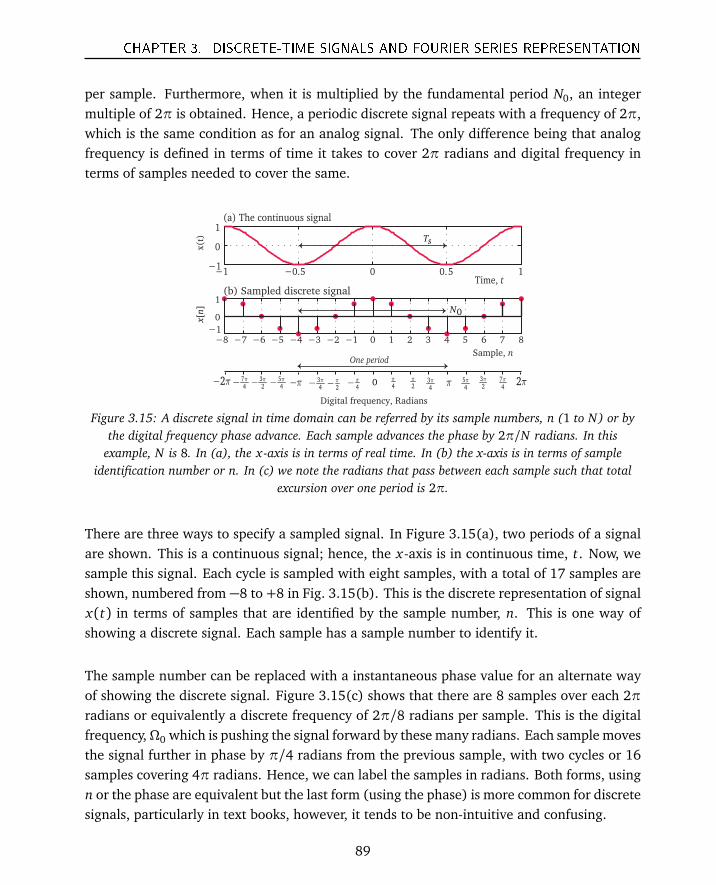
CHAPTER 3. DISCRETE-TIME SIGNALS AND FOURIER SERIES REPRESENTATION
per sample. Furthermore, when it is multiplied by the fundamental period N0, an integermultiple of 2π is obtained. Hence, a periodic discrete signal repeats with a frequency of 2π,which is the same condition as for an analog signal. The only difference being that analogfrequency is defined in terms of time it takes to cover 2π radians and digital frequency interms of samples needed to cover the same.
−1 −0.5 0 0.5 1−1
0
1
Time, t
x(t
)
(a) The continuous signal
−8 −7 −6 −5 −4 −3 −2 −1 0 1 2 3 4 5 6 7 8−1
0
1(b) Sampled discrete signal
Sample, n
0 2π2π−4π
4π
−2π
− 2π
ππ−
Digital frequency, Radians
34π
−34π
[]
xn
32π3
2π
−
54π
−54π 7
4π7
4π
−
sT
0N
One period
Figure 3.15: A discrete signal in time domain can be referred by its sample numbers, n (1 to N) or bythe digital frequency phase advance. Each sample advances the phase by 2π/N radians. In this
example, N is 8. In (a), the x-axis is in terms of real time. In (b) the x-axis is in terms of sampleidentification number or n. In (c) we note the radians that pass between each sample such that total
excursion over one period is 2π.
There are three ways to specify a sampled signal. In Figure 3.15(a), two periods of a signalare shown. This is a continuous signal; hence, the x-axis is in continuous time, t. Now, wesample this signal. Each cycle is sampled with eight samples, with a total of 17 samples areshown, numbered from −8 to +8 in Fig. 3.15(b). This is the discrete representation of signalx(t) in terms of samples that are identified by the sample number, n. This is one way ofshowing a discrete signal. Each sample has a sample number to identify it.
The sample number can be replaced with a instantaneous phase value for an alternate wayof showing the discrete signal. Figure 3.15(c) shows that there are 8 samples over each 2πradians or equivalently a discrete frequency of 2π/8 radians per sample. This is the digitalfrequency,Ω0 which is pushing the signal forward by these many radians. Each sample movesthe signal further in phase by π/4 radians from the previous sample, with two cycles or 16samples covering 4π radians. Hence, we can label the samples in radians. Both forms, usingn or the phase are equivalent but the last form (using the phase) is more common for discretesignals, particularly in text books, however, it tends to be non-intuitive and confusing.
89
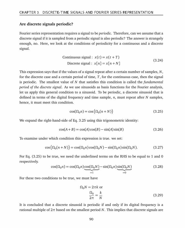
CHAPTER 3. DISCRETE-TIME SIGNALS AND FOURIER SERIES REPRESENTATION
Are discrete signals periodic?
Fourier series representation requires a signal to be periodic. Therefore, can we assume that adiscrete signal if it is sampled from a periodic signal is also periodic? The answer is strangelyenough, no. Here, we look at the conditions of periodicity for a continuous and a discretesignal.
Continuous signal : x(t) = x(t + T )
Discrete signal : x[n] = x[n+ N](3.24)
This expression says that if the values of a signal repeat after a certain number of samples, N ,for the discrete case and a certain period of time, T , for the continuous case, then the signalis periodic. The smallest value of N that satisfies this condition is called the fundamentalperiod of the discrete signal. As we use sinusoids as basis functions for the Fourier analysis,let us apply this general condition to a sinusoid. To be periodic, a discrete sinusoid that isdefined in terms of the digital frequency and time sample, n, must repeat after N samples,hence, it must meet this condition.
cos(Ω0n) = cos
Ω0(n+ N)
(3.25)
We expand the right-hand-side of Eq. 3.25 using this trigonometric identity:
cos(A+ B) = cos(A) cos(B)− sin(A) sin(B) (3.26)
To examine under which condition this expression is true. we set:
cos
Ω0(n+ N)
= cos(Ω0n) cos(Ω0N)− sin(Ω0n) sin(Ω0N). (3.27)
For Eq. (3.25) to be true, we need the underlined terms on the RHS to be equal to 1 and 0respectively.
cos(Ω0n) = cos(Ω0n) cos(Ω0N)︸ ︷︷ ︸
=1
− sin(Ω0n) sin(Ω0N)︸ ︷︷ ︸
=0
(3.28)
For these two conditions to be true, we must have
Ω0N = 2πk or
Ω0
2π=
kN
(3.29)
It is concluded that a discrete sinusoid is periodic if and only if its digital frequency is arational multiple of 2π based on the smallest period N . This implies that discrete signals are
90
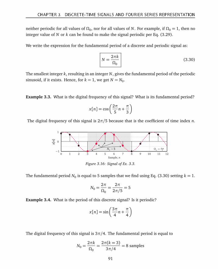
CHAPTER 3. DISCRETE-TIME SIGNALS AND FOURIER SERIES REPRESENTATION
neither periodic for all values of Ω0, nor for all values of N . For example, if Ω0 = 1, then nointeger value of N or k can be found to make the signal periodic per Eq. (3.29).
We write the expression for the fundamental period of a discrete and periodic signal as:
N =2πkΩ0
(3.30)
The smallest integer k, resulting in an integer N , gives the fundamental period of the periodicsinusoid, if it exists. Hence, for k = 1, we get N = N0.
Example 3.3. What is the digital frequency of this signal? What is its fundamental period?
x[n] = cos
2π5
n+π
3
The digital frequency of this signal is 2π/5 because that is the coefficient of time index n.
0 2 4 6 8 10 12−1
0
1
Sample, n
1 3 5 7 9 11
0 5N =
[]
xn
25
n
n
πΩ =
Figure 3.16: Signal of Ex. 3.3.
The fundamental period N0 is equal to 5 samples that we find using Eq. (3.30) setting k = 1.
N0 =2πΩ0=
2π2π/5
= 5
Example 3.4. What is the period of this discrete signal? Is it periodic?
x[n] = sin
3π4
n+π
4
The digital frequency of this signal is 3π/4. The fundamental period is equal to
N0 =2πkΩ0=
2π(k = 3)3π/4
= 8 samples
91
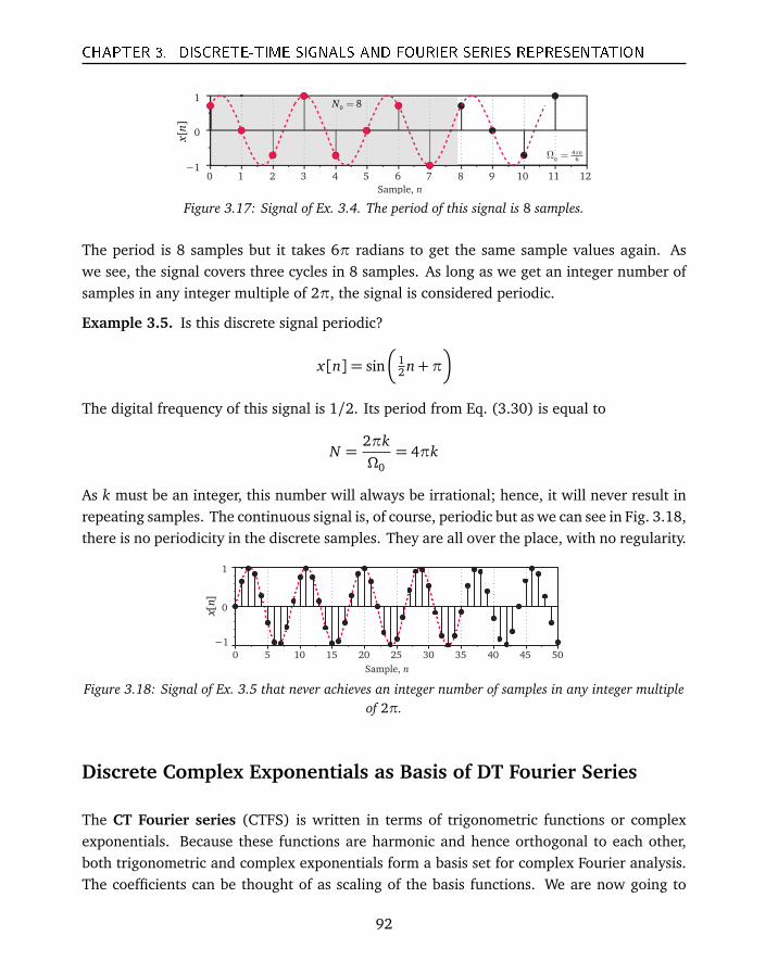
CHAPTER 3. DISCRETE-TIME SIGNALS AND FOURIER SERIES REPRESENTATION
0 1 2 3 4 5 6 7 8 9 10 11 12−1
0
1
Sample, n[]
xn
0 8N =
46
n
n
π
Ω =
Figure 3.17: Signal of Ex. 3.4. The period of this signal is 8 samples.
The period is 8 samples but it takes 6π radians to get the same sample values again. Aswe see, the signal covers three cycles in 8 samples. As long as we get an integer number ofsamples in any integer multiple of 2π, the signal is considered periodic.
Example 3.5. Is this discrete signal periodic?
x[n] = sin
12 n+π
The digital frequency of this signal is 1/2. Its period from Eq. (3.30) is equal to
N =2πkΩ0= 4πk
As k must be an integer, this number will always be irrational; hence, it will never result inrepeating samples. The continuous signal is, of course, periodic but as we can see in Fig. 3.18,there is no periodicity in the discrete samples. They are all over the place, with no regularity.
0 5 10 15 20 25 30 35 40 45 50
−1
0
1
Sample, n
[]
xn
Figure 3.18: Signal of Ex. 3.5 that never achieves an integer number of samples in any integer multipleof 2π.
Discrete Complex Exponentials as Basis of DT Fourier Series
The CT Fourier series (CTFS) is written in terms of trigonometric functions or complexexponentials. Because these functions are harmonic and hence orthogonal to each other,both trigonometric and complex exponentials form a basis set for complex Fourier analysis.The coefficients can be thought of as scaling of the basis functions. We are now going to
92
CHAPTER 3. DISCRETE-TIME SIGNALS AND FOURIER SERIES REPRESENTATION
look at the Fourier series representation for DT signals using DT complex exponentials as thebasis functions.
A discrete complex exponential is written by replacing t in CT domain with n, and ω withthe digital frequency Ω. Now, we have these two forms of the CE just as we wrote the twoforms of the sinusoid in Eq. (3.22).
Continuous form of a CE : e jω0 t
Discrete form of a CE : e jΩ0n
The discrete form of the fundamental is expanded as follows. We show a single CE of digitalfrequency 2π
N for variable n, the DT index of time. The harmonic factor k has not yet beenincluded in this equation.
e jΩ0n = e j
2πN
n (3.31)
Harmonics of a discrete fundamental CE
For an analog signal, we define its harmonics by multiplying its frequency directly by amultiplier k. Can we do the same for discrete signals? Do we just multiply the fundamentalfrequency by the index k, such as 2kπ/N for all k? Well, no. If a signal has fundamentaldigital frequency of π/5, then is frequency 2π/5 the next harmonic? Yes, and no, becausethis method leads us into problems.
The range of the digital frequency is 2π. To obtain its next harmonic, we increment itsfrequency by adding an integer multiple of 2π to it. Hence, the frequency of a kth harmonicof a discrete signal is (Ω0 + 2πk) or (π/5+2π) = 12π/5 for k = 1. This is a very importantpoint. The analog and discrete harmonics have equivalent definitions for purposes of theFourier analysis. We will see, however, that they do not display the same behavior. Wecannot use these traditionally defined discrete harmonics for the Fourier analysis.
Discrete fundamental : e j(2π/N)n
Discrete harmonic : e j(2π/N+2πk)n
Repeating harmonics of a discrete signal
Where each and every harmonic of an analog signal looks different, i.e., has higher frequency,shows more ups and downs, etc., the discrete harmonics defined by e j(2π/N+2πk)n for each k
93
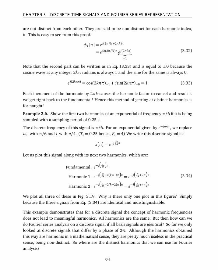
CHAPTER 3. DISCRETE-TIME SIGNALS AND FOURIER SERIES REPRESENTATION
are not distinct from each other. They are said to be non-distinct for each harmonic index,k. This is easy to see from this proof.
φk[n] = e j(2π/N+2πk)n
= e jk(2π/N)n e j(2πkn)︸ ︷︷ ︸
=1
(3.32)
Note that the second part can be written as in Eq. (3.33) and is equal to 1.0 because thecosine wave at any integer 2kπ radians is always 1 and the sine for the same is always 0.
e j(2kπn) = cos(2knπ)=1 + jsin(2knπ)=0 = 1 (3.33)
Each increment of the harmonic by 2πk causes the harmonic factor to cancel and result iswe get right back to the fundamental! Hence this method of getting at distinct harmonics isfor naught!
Example 3.6. Show the first two harmonics of an exponential of frequency π/6 if it is beingsampled with a sampling period of 0.25 s.
The discrete frequency of this signal is π/6. For an exponential given by e− jω0 t , we replaceω0 with π/6 and t with n/4. (Ts = 0.25 hence, Fs = 4) We write this discrete signal as:
x[n] = e− j 2π24 n
Let us plot this signal along with its next two harmonics, which are:
Fundamental : e− j
π24
n
Harmonic 1 : e− j
π24+2(k=1)π
n = e− j
π24+2π
n
Harmonic 2 : e− j
π24+2(k=2)π
n = e− j
π24+4π
n
(3.34)
We plot all three of these in Fig. 3.19. Why is there only one plot in this figure? Simplybecause the three signals from Eq. (3.34) are identical and indistinguishable.
This example demonstrates that for a discrete signal the concept of harmonic frequenciesdoes not lead to meaningful harmonics. All harmonics are the same. But then how can wedo Fourier series analysis on a discrete signal if all basis signals are identical? So far we onlylooked at discrete signals that differ by a phase of 2π. Although the harmonics obtainedthis way are harmonic in a mathematical sense, they are pretty much useless in the practicalsense, being non-distinct. So where are the distinct harmonics that we can use for Fourieranalysis?
94
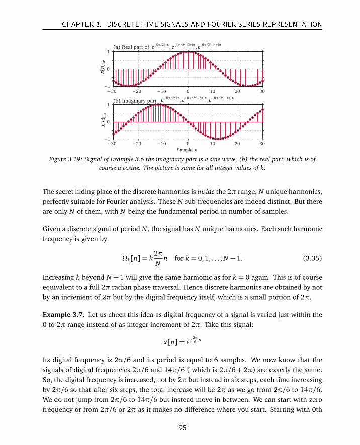
CHAPTER 3. DISCRETE-TIME SIGNALS AND FOURIER SERIES REPRESENTATION
−30 −20 −10 0 10 20 30−1
0
1
−30 −20 −10 0 10 20 30−1
0
1
Sample, n
(a) Real part of
(b) Imaginary part R
e[
]x
nIm
[]
xn
( /24)n ( /24 2 )n ( /24 4 )n, ,j j je e e
π π π π π− − + − +
( /24)n ( /24 2 )n ( /24 4 )n, ,j j je e e
π π π π π− − + − +
Figure 3.19: Signal of Example 3.6 the imaginary part is a sine wave, (b) the real part, which is ofcourse a cosine. The picture is same for all integer values of k.
The secret hiding place of the discrete harmonics is inside the 2π range, N unique harmonics,perfectly suitable for Fourier analysis. These N sub-frequencies are indeed distinct. But thereare only N of them, with N being the fundamental period in number of samples.
Given a discrete signal of period N , the signal has N unique harmonics. Each such harmonicfrequency is given by
Ωk[n] = k2πN
n for k = 0,1, . . . , N − 1. (3.35)
Increasing k beyond N − 1 will give the same harmonic as for k = 0 again. This is of courseequivalent to a full 2π radian phase traversal. Hence discrete harmonics are obtained by notby an increment of 2π but by the digital frequency itself, which is a small portion of 2π.
Example 3.7. Let us check this idea as digital frequency of a signal is varied just within the0 to 2π range instead of as integer increment of 2π. Take this signal:
x[n] = e j 2π6 n
Its digital frequency is 2π/6 and its period is equal to 6 samples. We now know that thesignals of digital frequencies 2π/6 and 14π/6 ( which is 2π/6+ 2π) are exactly the same.So, the digital frequency is increased, not by 2π but instead in six steps, each time increasingby 2π/6 so that after six steps, the total increase will be 2π as we go from 2π/6 to 14π/6.We do not jump from 2π/6 to 14π/6 but instead move in between. We can start with zerofrequency or from 2π/6 or 2π as it makes no difference where you start. Starting with 0th
95
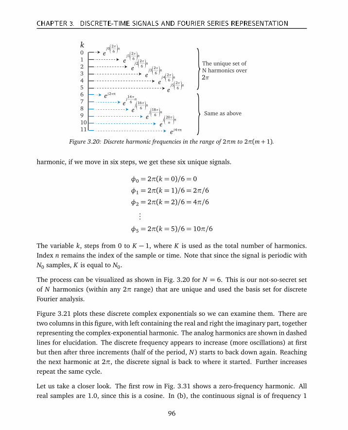
CHAPTER 3. DISCRETE-TIME SIGNALS AND FOURIER SERIES REPRESENTATION
k0
1
2
3
4
5
6
7
8
9
10
11
20
6j n
e
π 2
16
j n
e
π
23
6j n
e
π 2
46
j n
e
π 2
56
j n
e
π
2j neπ
14
6j n
e
π
22
6j n
e
π
16
6j n
e
π 18
6j n
e
π
4j neπ
20j n
ne
π
The unique set of
N harmonics over
2π
Same as above
Figure 3.20: Discrete harmonic frequencies in the range of 2πm to 2π(m+ 1).
harmonic, if we move in six steps, we get these six unique signals.
φ0 = 2π(k = 0)/6= 0
φ1 = 2π(k = 1)/6= 2π/6
φ2 = 2π(k = 2)/6= 4π/6...
φ5 = 2π(k = 5)/6= 10π/6
The variable k, steps from 0 to K − 1, where K is used as the total number of harmonics.Index n remains the index of the sample or time. Note that since the signal is periodic withN0 samples, K is equal to N0.
The process can be visualized as shown in Fig. 3.20 for N = 6. This is our not-so-secret setof N harmonics (within any 2π range) that are unique and used the basis set for discreteFourier analysis.
Figure 3.21 plots these discrete complex exponentials so we can examine them. There aretwo columns in this figure, with left containing the real and right the imaginary part, togetherrepresenting the complex-exponential harmonic. The analog harmonics are shown in dashedlines for elucidation. The discrete frequency appears to increase (more oscillations) at firstbut then after three increments (half of the period, N) starts to back down again. Reachingthe next harmonic at 2π, the discrete signal is back to where it started. Further increasesrepeat the same cycle.
Let us take a closer look. The first row in Fig. 3.31 shows a zero-frequency harmonic. Allreal samples are 1.0, since this is a cosine. In (b), the continuous signal is of frequency 1
96
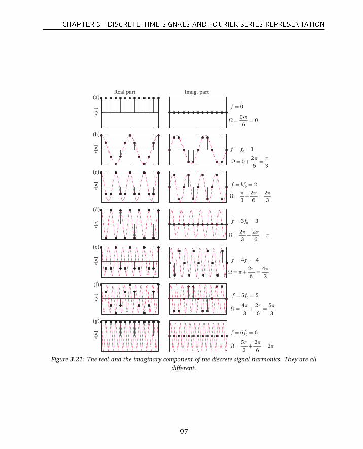
CHAPTER 3. DISCRETE-TIME SIGNALS AND FOURIER SERIES REPRESENTATION
Real part Imag. part
00
6
π
Ω= =i
0f =
20
6 3
π π
Ω= + =
2 2
3 6 3
π π π
Ω= + =
2 2
3 6
π π
πΩ= + =
2 4
6 3
π π
πΩ= + =
4 2 5
3 6 3
π π π
Ω= + =
5 22
3 6
π π
πΩ= + =
0 1f f= =
0 2f kf= =
03 3f f= =
04 4f f= =
05 5f f= =
06 6f f= =
(a)
(b)
(c)
(d)
(e)
(f)
(g)
[]
xn
[]
xn
[]
xn
[]
xn
[]
xn
[]
xn
[]
xn
Figure 3.21: The real and the imaginary component of the discrete signal harmonics. They are alldifferent.
97
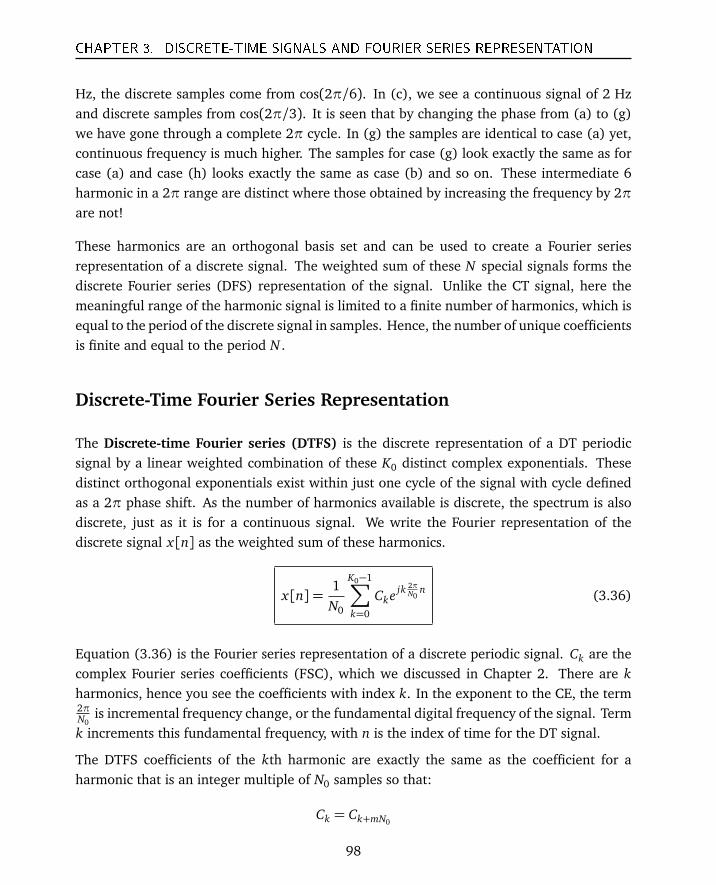
CHAPTER 3. DISCRETE-TIME SIGNALS AND FOURIER SERIES REPRESENTATION
Hz, the discrete samples come from cos(2π/6). In (c), we see a continuous signal of 2 Hzand discrete samples from cos(2π/3). It is seen that by changing the phase from (a) to (g)we have gone through a complete 2π cycle. In (g) the samples are identical to case (a) yet,continuous frequency is much higher. The samples for case (g) look exactly the same as forcase (a) and case (h) looks exactly the same as case (b) and so on. These intermediate 6harmonic in a 2π range are distinct where those obtained by increasing the frequency by 2πare not!
These harmonics are an orthogonal basis set and can be used to create a Fourier seriesrepresentation of a discrete signal. The weighted sum of these N special signals forms thediscrete Fourier series (DFS) representation of the signal. Unlike the CT signal, here themeaningful range of the harmonic signal is limited to a finite number of harmonics, which isequal to the period of the discrete signal in samples. Hence, the number of unique coefficientsis finite and equal to the period N .
Discrete-Time Fourier Series Representation
The Discrete-time Fourier series (DTFS) is the discrete representation of a DT periodicsignal by a linear weighted combination of these K0 distinct complex exponentials. Thesedistinct orthogonal exponentials exist within just one cycle of the signal with cycle definedas a 2π phase shift. As the number of harmonics available is discrete, the spectrum is alsodiscrete, just as it is for a continuous signal. We write the Fourier representation of thediscrete signal x[n] as the weighted sum of these harmonics.
x[n] =1N0
K0−1∑
k=0
Cke jk 2πN0
n (3.36)
Equation (3.36) is the Fourier series representation of a discrete periodic signal. Ck are thecomplex Fourier series coefficients (FSC), which we discussed in Chapter 2. There are kharmonics, hence you see the coefficients with index k. In the exponent to the CE, the term2πN0
is incremental frequency change, or the fundamental digital frequency of the signal. Termk increments this fundamental frequency, with n is the index of time for the DT signal.
The DTFS coefficients of the kth harmonic are exactly the same as the coefficient for aharmonic that is an integer multiple of N0 samples so that:
Ck = Ck+mN0
98
CHAPTER 3. DISCRETE-TIME SIGNALS AND FOURIER SERIES REPRESENTATION
The Inverse DTFSC equation is given by the kth coefficient and hence, the kth coefficient isgiven by
Ck =N0−1∑
n=0
x[n]e− jΩ0nk (3.37)
The (k+mK0)th coefficient is given by
Ck+mK0=
N0−1∑
n=0
x[n]e− j(k+mN0)Ω0n
=N0−1∑
n=0
x[n]e− jkΩ0ne− jmN0Ω0n
The second part of the signal is equal to 1.
e− jmN0Ω0n = e− jm2πn = 1
(Because the value of the complex exponential at integer multiples of 2π is equal to 1.0).Therefore, we have:
Ck+mN0=
N0−1∑
n=0
x[n]e− j(k+mK0)Ω0n = Ck (3.38)
This says that the harmonics repeat, and hence the coefficients also repeat. The spectrum ofthe discrete signal (comprising the coefficients) keeps repeating after every integer multipleof the K0 samples, or by the sampling frequency. In practical sense, this means we can limitthe computation to just the first K0 harmonics, where, K0 is equal to N0.
This is a very different situation from the continuous signals, which do not have such behavior.The CT coefficients are unique for all values of k.
DTFS Examples
Example 3.8. Find the DT Fourier series coefficients of this signal.
x[k] = 1+ sin
2π10
k
The fundamental period of this signal is equal to 10 samples from observation. Hence, it canonly have at most 10 unique coefficients.
99
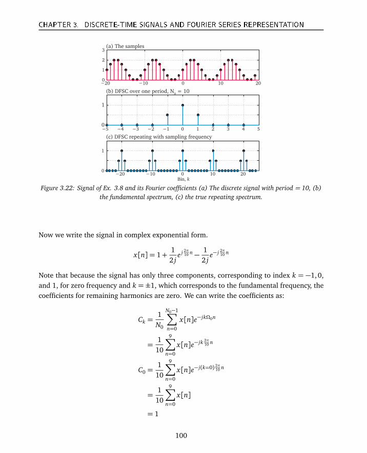
CHAPTER 3. DISCRETE-TIME SIGNALS AND FOURIER SERIES REPRESENTATION
−20 −10 0 10 200
1
2
3
−5 −4 −3 −2 −1 0 1 2 3 4 50
1
−20 −10 0 10 200
1
(a) The samples
(b) DFSC over one period, N0 = 10
(c) DFSC repeating with sampling frequency
Bin, k
Figure 3.22: Signal of Ex. 3.8 and its Fourier coefficients (a) The discrete signal with period = 10, (b)the fundamental spectrum, (c) the true repeating spectrum.
Now we write the signal in complex exponential form.
x[n] = 1+12 j
e j 2π10 n −
12 j
e− j 2π10 n
Note that because the signal has only three components, corresponding to index k = −1,0,and 1, for zero frequency and k = ±1, which corresponds to the fundamental frequency, thecoefficients for remaining harmonics are zero. We can write the coefficients as:
Ck =1N0
N0−1∑
n=0
x[n]e− jkΩ0n
=1
10
9∑
n=0
x[n]e− jk 2π10 n
C0 =1
10
9∑
n=0
x[n]e− j(k=0) 2π10 n
=1
10
9∑
n=0
x[n]
= 1
100
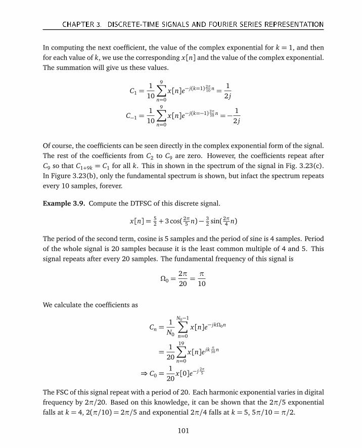
CHAPTER 3. DISCRETE-TIME SIGNALS AND FOURIER SERIES REPRESENTATION
In computing the next coefficient, the value of the complex exponential for k = 1, and thenfor each value of k, we use the corresponding x[n] and the value of the complex exponential.The summation will give us these values.
C1 =110
9∑
n=0
x[n]e− j(k=1) 2π10 n =
12 j
C−1 =110
9∑
n=0
x[n]e− j(k=−1) 2π10 n = −
12 j
Of course, the coefficients can be seen directly in the complex exponential form of the signal.The rest of the coefficients from C2 to C9 are zero. However, the coefficients repeat afterC9 so that C1+9k = C1 for all k. This in shown in the spectrum of the signal in Fig. 3.23(c).In Figure 3.23(b), only the fundamental spectrum is shown, but infact the spectrum repeatsevery 10 samples, forever.
Example 3.9. Compute the DTFSC of this discrete signal.
x[n] = 52 + 3cos(2π
5 n)− 32 sin(2π
4 n)
The period of the second term, cosine is 5 samples and the period of sine is 4 samples. Periodof the whole signal is 20 samples because it is the least common multiple of 4 and 5. Thissignal repeats after every 20 samples. The fundamental frequency of this signal is
Ω0 =2π20=π
10
We calculate the coefficients as
Cn =1N0
N0−1∑
n=0
x[n]e− jkΩ0n
=120
19∑
n=0
x[n]e jk π10 n
⇒ C0 =120
x[0]e− j 2π5
The FSC of this signal repeat with a period of 20. Each harmonic exponential varies in digitalfrequency by 2π/20. Based on this knowledge, it can be shown that the 2π/5 exponentialfalls at k = 4, 2(π/10) = 2π/5 and exponential 2π/4 falls at k = 5, 5π/10= π/2.
101
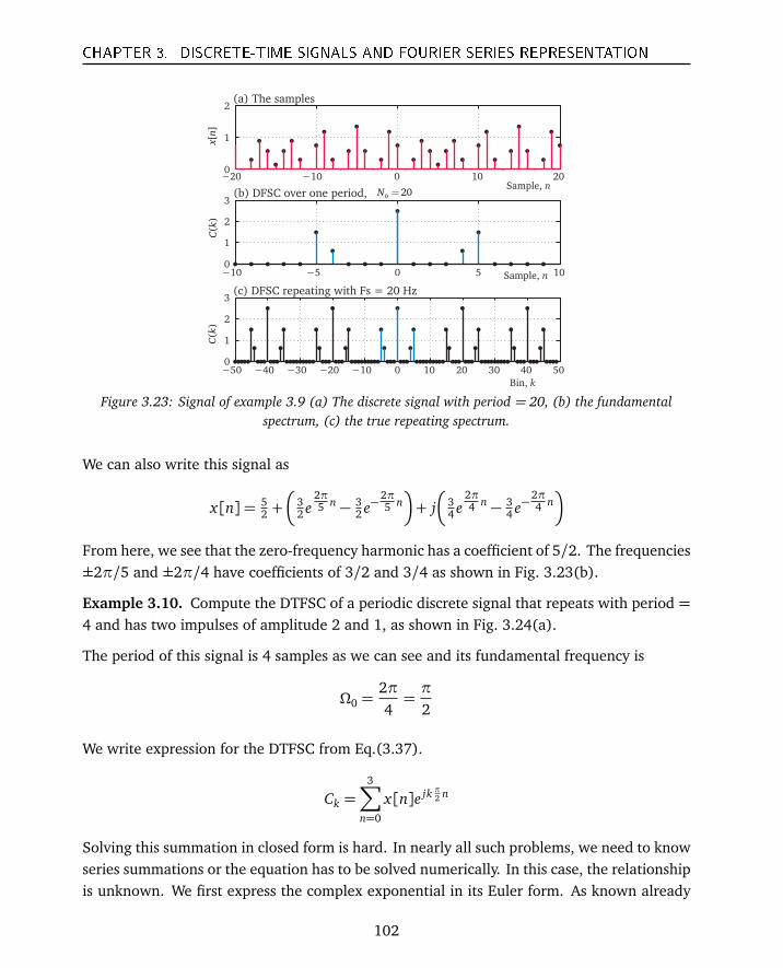
CHAPTER 3. DISCRETE-TIME SIGNALS AND FOURIER SERIES REPRESENTATION
−20 −10 0 10 200
1
2
Sample, n
−10 −5 0 5 100
1
2
3
−50 −40 −30 −20 −10 0 10 20 30 40 500
1
2
3
(a) The samples
(b) DFSC over one period,
(c) DFSC repeating with Fs = 20 Hz
[]
xn
()
Ck
()
Ck
0 20N =
Sample, n
Bin, k
Figure 3.23: Signal of example 3.9 (a) The discrete signal with period = 20, (b) the fundamentalspectrum, (c) the true repeating spectrum.
We can also write this signal as
x[n] = 52 +
32 e
2π5 n − 3
2 e−2π5 n
+ j
34 e
2π4 n − 3
4 e−2π4 n
From here, we see that the zero-frequency harmonic has a coefficient of 5/2. The frequencies±2π/5 and ±2π/4 have coefficients of 3/2 and 3/4 as shown in Fig. 3.23(b).
Example 3.10. Compute the DTFSC of a periodic discrete signal that repeats with period =4 and has two impulses of amplitude 2 and 1, as shown in Fig. 3.24(a).
The period of this signal is 4 samples as we can see and its fundamental frequency is
Ω0 =2π4=π
2
We write expression for the DTFSC from Eq.(3.37).
Ck =3∑
n=0
x[n]e jk π2 n
Solving this summation in closed form is hard. In nearly all such problems, we need to knowseries summations or the equation has to be solved numerically. In this case, the relationshipis unknown. We first express the complex exponential in its Euler form. As known already
102
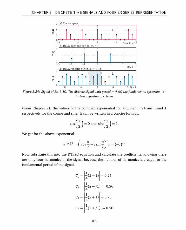
CHAPTER 3. DISCRETE-TIME SIGNALS AND FOURIER SERIES REPRESENTATION
−10 −5 0 5 100
1
2
3
−3 −2 −1 0 1 2 30
1
−8 −4 0 4 80
1
(a) The samples
(b) DFSC over one period,
(c) DFSC repeating with Fs = 4 Hz
0 4N =
[]
xn
()
Ck
()
Ck
Sample, n
Bin, k
Bin, k
Figure 3.24: Signal of Ex. 3.10. The discrete signal with period = 4 (b) the fundamental spectrum, (c)the true repeating spectrum.
(from Chapter 2), the values of the complex exponential for argument π/4 are 0 and 1respectively for the cosine and sine. It can be written in a concise form as:
cos
π
2
= 0 and sin
π
2
= 1.
We get for the above exponential
e− jnπ2 k =
cosπ
2− j sin
π
2
n
k = (− j)nk
Now substitute this into the DTFSC equation and calculate the coefficients, knowing thereare only four harmonics in the signal because the number of harmonics are equal to thefundamental period of the signal.
C0 =
14(2− 1)
= 0.25
C1 =
14(2− j1)
= 0.56
C2 =
14(2+ 1)
= 0.75
C3 =
14(2+ j1)
= 0.56
103
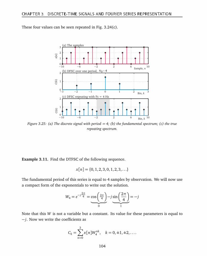
CHAPTER 3. DISCRETE-TIME SIGNALS AND FOURIER SERIES REPRESENTATION
These four values can be seen repeated in Fig. 3.24(c).
−10 −6 −2 2 6 100
1
2
3
−3 −2 −1 0 1 2 30
1
2
−10 −6 −2 2 6 100
1
2
(a) The samples
(b) DFSC over one period,
(c) DFSC repeating with Fs = 4 Hz
0 4N =
()
Ck
()
Ck
[]
xn
Sample, n
Bin, k
Bin, k
Figure 3.25: (a) The discrete signal with period = 4; (b) the fundamental spectrum; (c) the truerepeating spectrum.
Example 3.11. Find the DTFSC of the following sequence.
x[n] = 0, 1,2,3, 0,1, 2,3, . . .
The fundamental period of this series is equal to 4 samples by observation. We will now usea compact form of the exponentials to write out the solution.
W4 = e− j2π4 = cos
2π4
︸ ︷︷ ︸
0
− j sin
2π4
︸ ︷︷ ︸
1
= − j
Note that this W is not a variable but a constant. Its value for these parameters is equal to− j. Now we write the coefficients as
Ck =3∑
n=0
x[n]W nk4 , k = 0,±1,±2, . . . .
104
CHAPTER 3. DISCRETE-TIME SIGNALS AND FOURIER SERIES REPRESENTATION
From here we get
C0 =3∑
n=0
x[n]W 0·n4 = 0+ 1+ 2+ 3= 6
C1 =3∑
n=0
x[n]W 1·n4 =
3∑
k=0
x[n](− j)n = 0− j − 2+ j3= −2+ j2
C2 =3∑
n=0
x[n]W 2·n4 =
3∑
k=0
x[n](− j)2n = −2
C3 =3∑
n=0
x[n]W 3·n4 =
3∑
k=0
x[n](− j)3n = −2− j2.
DTFSC of a repeating square pulse signal
Example 3.12. Find the DTFSC of a square pulse signal of width L samples and period N .
Once again, we examine the FSC of a square pulse signal. The signal is discrete now, whichmeans that it has a certain number of non-zero samples along with the zeros for the rest,making up one period of DT data. We set the period of the pulse to L samples, which is thewidth of the pulse. The length of the period is N samples. The duty cycle is defined as theratio of the pulse width, L and the period, N . The pulse is not centered at the origin in thiscase, as shown in Fig. 3.26. This has the effect of introducing a phase term, as we shall seein the result.
To compute the DTFSC, the following important property of geometric series is used.
M∑
n=0
an =1− aM
1− a, |a|< 1. (3.39)
105
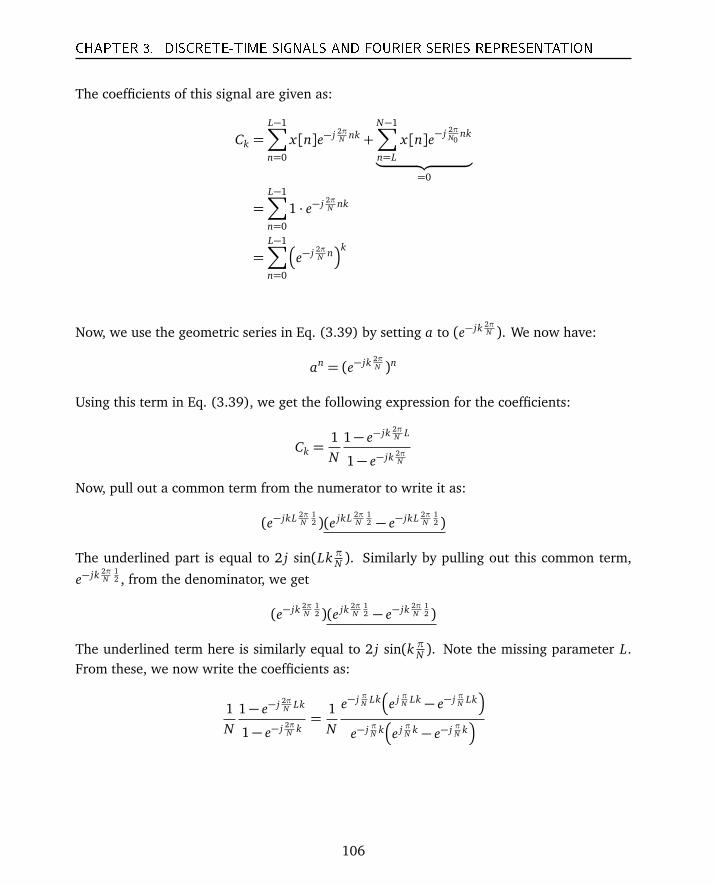
CHAPTER 3. DISCRETE-TIME SIGNALS AND FOURIER SERIES REPRESENTATION
The coefficients of this signal are given as:
Ck =L−1∑
n=0
x[n]e− j 2πN nk +
N−1∑
n=L
x[n]e− j 2πN0
nk
︸ ︷︷ ︸
=0
=L−1∑
n=0
1 · e− j 2πN nk
=L−1∑
n=0
e− j 2πN nk
Now, we use the geometric series in Eq. (3.39) by setting a to (e− jk 2πN ). We now have:
an = (e− jk 2πN )n
Using this term in Eq. (3.39), we get the following expression for the coefficients:
Ck =1N
1− e− jk 2πN L
1− e− jk 2πN
Now, pull out a common term from the numerator to write it as:
(e− jkL 2πN
12 )(e jkL 2π
N12 − e− jkL 2π
N12 )
The underlined part is equal to 2 j sin(Lk πN ). Similarly by pulling out this common term,
e− jk 2πN
12 , from the denominator, we get
(e− jk 2πN
12 )(e jk 2π
N12 − e− jk 2π
N12 )
The underlined term here is similarly equal to 2 j sin(k πN ). Note the missing parameter L.From these, we now write the coefficients as:
1N
1− e− j 2πN Lk
1− e− j 2πN k=
1N
e− j πN Lk
e j πN Lk − e− j πN Lk
e− j πN k
e j πN k − e− j πN k
106
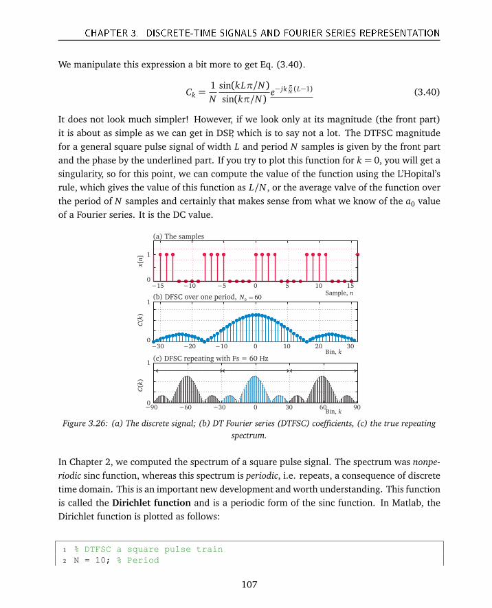
CHAPTER 3. DISCRETE-TIME SIGNALS AND FOURIER SERIES REPRESENTATION
We manipulate this expression a bit more to get Eq. (3.40).
Ck =1N
sin(kLπ/N)sin(kπ/N)
e− jk πN (L−1) (3.40)
It does not look much simpler! However, if we look only at its magnitude (the front part)it is about as simple as we can get in DSP, which is to say not a lot. The DTFSC magnitudefor a general square pulse signal of width L and period N samples is given by the front partand the phase by the underlined part. If you try to plot this function for k = 0, you will get asingularity, so for this point, we can compute the value of the function using the L’Hopital’srule, which gives the value of this function as L/N , or the average valve of the function overthe period of N samples and certainly that makes sense from what we know of the a0 valueof a Fourier series. It is the DC value.
−15 −10 −5 0 5 10 150
1
−30 −20 −10 0 10 20 300
−90 −60 −30 0 30 60 900
1
1
[]
xn
()
Ck
()
Ck
(a) The samples
(b) DFSC over one period,
(c) DFSC repeating with Fs = 60 Hz
0 60N =
Sample, n
Bin, k
Bin, k
Figure 3.26: (a) The discrete signal; (b) DT Fourier series (DTFSC) coefficients, (c) the true repeatingspectrum.
In Chapter 2, we computed the spectrum of a square pulse signal. The spectrum was nonpe-riodic sinc function, whereas this spectrum is periodic, i.e. repeats, a consequence of discretetime domain. This is an important new development and worth understanding. This functionis called the Dirichlet function and is a periodic form of the sinc function. In Matlab, theDirichlet function is plotted as follows:
1 % DTFSC a square pulse train2 N = 10; % Period
107
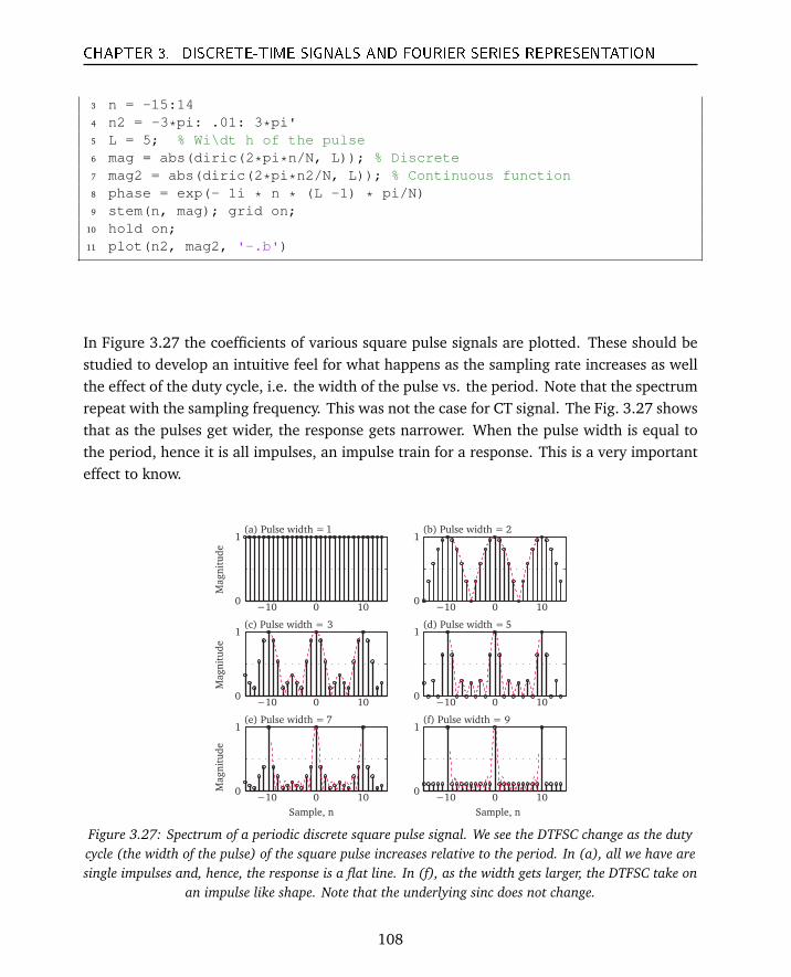
CHAPTER 3. DISCRETE-TIME SIGNALS AND FOURIER SERIES REPRESENTATION
3 n = -15:144 n2 = -3*pi: .01: 3*pi'5 L = 5; % Wi\dt h of the pulse6 mag = abs(diric(2*pi*n/N, L)); % Discrete7 mag2 = abs(diric(2*pi*n2/N, L)); % Continuous function8 phase = exp(- 1i * n * (L -1) * pi/N)9 stem(n, mag); grid on;
10 hold on;11 plot(n2, mag2, '-.b')
In Figure 3.27 the coefficients of various square pulse signals are plotted. These should bestudied to develop an intuitive feel for what happens as the sampling rate increases as wellthe effect of the duty cycle, i.e. the width of the pulse vs. the period. Note that the spectrumrepeat with the sampling frequency. This was not the case for CT signal. The Fig. 3.27 showsthat as the pulses get wider, the response gets narrower. When the pulse width is equal tothe period, hence it is all impulses, an impulse train for a response. This is a very importanteffect to know.
−10 0 100
1(a) Pulse width = 1
−10 0 100
1(b) Pulse width = 2
−10 0 100
1(c) Pulse width = 3
−10 0 100
1(d) Pulse width = 5
−10 0 100
1(e) Pulse width = 7
−10 0 100
1(f) Pulse width = 9
Sample, n Sample, n
Magn
itu
de
Magn
itu
de
Magn
itu
de
Figure 3.27: Spectrum of a periodic discrete square pulse signal. We see the DTFSC change as the dutycycle (the width of the pulse) of the square pulse increases relative to the period. In (a), all we have aresingle impulses and, hence, the response is a flat line. In (f), as the width gets larger, the DTFSC take on
an impulse like shape. Note that the underlying sinc does not change.
108
CHAPTER 3. DISCRETE-TIME SIGNALS AND FOURIER SERIES REPRESENTATION
Power spectrum
In all the examples in this chapter, we have been plotting either the magnitude or the amplitudespectrum. The Power spectrum is a different thing. As per the Parseval’s theorem, it is definedas:
∞∑
n=−∞|x[n]|2 =
∞∑
k=−∞
X [ Fsn k]
2(3.41)
Similar to the idea from circuits, to obtain power, we square the time-domain sample amplitudeto obtain the instantaneous power at that time instant. If the unit of the amplitude is voltage,the units become voltage-squared. If all such individual squared-amplitudes are summed, weget the total power in the signal (assuming a unity resistance.) Alternately, we can sum thesquare of the coefficients of each harmonic. They have units of amplitude too. This alsogives us units of voltage-squared and can be used to convert a DTFSC into a Power spectrumby plotting the quantity (Ck)2 as a function of the index, k.
Matrix method for computing FSC
DTFSC are computed in closed-form for homework problems only. For practical applications,Matlab and other software and hardware devices are used. We will now look at a matrixmethod of computing the DTFSC.
Let us first define this common term. It looks strange and confusing, but it is a very simpleidea. We use it to separate out the constant terms.
WN0¬ e− j 2π
N0 . (3.42)
For a given N0, the signal period in samples, this term W , also called the Twiddle factor isa constant and is given a shorthand notation to make the equation writing easier. Using thisfactor, the DFS and the inverse DFS (IDFS) can be written as:
DFS: X [k] =N0−1∑
n=0
x[n]W nkN0
IDFS: x[n] =1N0
N0−1∑
k=0
X [k]W−nkN0
(3.43)
109
CHAPTER 3. DISCRETE-TIME SIGNALS AND FOURIER SERIES REPRESENTATION
In this form, the terms W nkN0
and W−nkN0
are same as:
W nkN0¬ e jk 2π
N0n
W−nkN0¬ e− jk 2π
N0n
These terms can be precomputed and stored to make computation quicker. They are the basicidea behind the FFT algorithm which speeds up computation. The DTFSC equation can besetup in matrix form using the Twiddle factor and writing it in terms of two variables, theindex n and k. Now we write:
Ck =1K0
x[n]
W−0×0 W−1×0 W−2×0 W−3×0
W−0×1 W−1×1 W−2×1 W−3×1
W−0×2 W−1×2 W−2×2 W−3×2
W−0×3 W−1×3 W−2×3 W−3×3
(3.44)
Here, we have assumed that N0 = 4. Each column represents the harmonic index k and eachrow the time index, n. It takes 16 exponentiations, 16 multiplications, and 4 summations tosolve this equation. We will come back to this matrix methodology again when we discussDFT and FFT in Chapter 6.
Summary of Chapter 3
In this chapter, we examined discrete signals, the requirements for sampling set by Shanonand Nyquist, and methods of reconstruction. Discrete signals can experience frequencyambiguity, as many analog frequencies can fit through the same samples. If not sampled ata rate higher then Nyquist rate, we get aliasing. The Fourier series representation of discretesignals uses discrete basis functions. If a discrete signal has a period of N samples, then itonly has N discrete harmonics within a 2π range. In this chapter, we developed the FSC fordiscrete signals and looked at the inverse process.
The terms we introduced in this chapter:
• Discrete signals - Defined only at specific uniform time intervals.• Digital signals - A discrete signals the amplitude of which is constrained to certain
values. A binary digital signal can only take on two values, 0 or 1.• Nyquist rate - Two times the maximum frequency in the signal.• Digital frequency - Measured in samples per radian.
110
CHAPTER 3. DISCRETE-TIME SIGNALS AND FOURIER SERIES REPRESENTATION
• Aliasing - Given a set of discrete samples, a frequency ambiguity exists, as infinitenumber of frequencies can pass through these samples. This effect is called aliasing.
• Discrete time Fourier series coefficients - DTFSC which repeat are the spectrum of adiscrete signal.
1. An ideal discrete signal is generated by sampling a continuous signal with an impulsetrain of desired sampling frequency. The time between the impulses is called the sampletime, and its inverse is called the sampling frequency.
2. The sampling frequency of an analog signal should be greater than two times thehighest frequency in the signal to accurately represent the signal.
3. The fundamental period of a discrete periodic signal, given by N0, must be an integernumber of samples for the signal to be periodic in a discrete sense.
4. The fundamental frequency (or digital frequency) of a discrete signal, given by Ω0, isequal to 2π/N0.
5. The period of the digital frequency is defined as any integer multiple of 2π. Harmonicdiscrete frequencies that vary by integer multiple of 2π, such as 2πk and 2πk+ 2πn,are identical.
6. We increment digital frequency by itself or 2π/N0, and use the N0 sub-frequenciesresulting as the basis set. These frequencies are harmonic and distinct.
7. There are only K0 harmonics available to represent a discrete signal. The number ofavailable harmonics for the Fourier representation, K0, is exactly equal to the fundamentalperiod of the signal, N0.
8. Beyond the 2π range of harmonic frequencies, the DT Fourier series coefficients, (DTFSC)repeat because the harmonics themselves are identical.
9. In contrast, the CT signal coefficients are aperiodic and do not repeat. This is becauseall harmonics of a continuous signal are unique.
10. The discrete Fourier series is written as:
x[n] =1N0
K0−1∑
k=0
Cke jk 2πN0
n
11. The coefficients of the DTFS are written as:
Ck =N0−1∑
n=0
x[n]e− jΩ0nk
12. The coefficients of a discrete periodic signal are discrete just as they are for the CTsignals.
111
CHAPTER 3. DISCRETE-TIME SIGNALS AND FOURIER SERIES REPRESENTATION
13. The coefficients around the zero frequency are called the principal fundamental aliasor principal spectrum.
14. The spectrum of a discrete periodic signal, repeats with sampling frequency, Fs.15. Sometimes, DTFSC coefficients can be solved using closed form solutions but in a
majority of the cases, matrix methods are used to find the coefficients of a signal.16. Matrix method is easy to set up but is computationally intensive. Fast matrix methods
are used to speed up the calculations. One such method is called FFT or Fast FourierTransform.
112
CHAPTER 3. DISCRETE-TIME SIGNALS AND FOURIER SERIES REPRESENTATION
Questions
1. Given this CT signal, being sampled at Fs = 25 Hz, write its discrete form. Is thesampling frequency above the Nyquist rate? x(t) = sin(2πt) + 0.5 cos(7πt)
2. If the largest frequency in a signal is f1 and the lowest is f2, then what is the minimumfrequency at which this signal should be sampled to be consistent with the Shannon’stheorem?
3. Why would a signal be sampled at a rate higher than two times its maximum frequency?4. A Gaussian signal does not have a clear maximum frequency. What frequency do you
choose for sampling such a signal?5. The bandwidth of a square pulse signal is infinite. How do you choose a sampling
frequency for such a signal? What can you do to reduce the bandwidth of this signal?6. For following three signals, what sampling frequency should be used so that it meets
the Nyquist rate.(a) x = cos(50t)(b) y = sin(30πt)(c) z = sin(31.4(t + 2))− cos(40πt)
7. What is the digital frequency of a signal given by these samples: x = [1 1 − 1 1].8. What is the fundamental period of a sinusoid cos(Ωn + φ), the digital frequency of
which is given by: 0.4π, 0.5π, 0.6π, and 0.75π.9. A discrete signal repeats after 37 samples. Is it periodic? A discrete signal repeats with
digital frequency of 2π/5, is it periodic?10. Stock data is noted every 5 s. What is its sampling frequency?11. Temperature is measured every 10 min during the day and every 15 min during the
night. 108 samples are collected over one day. Can we compute Fourier series coefficientsof this data?
12. A signal has a period of 8 samples. What is its fundamental digital frequency?13. Why would we want to recreate a signal from its samples?14. Are we able to transmit discrete data over an rf(analog) link?15. We have a sequence of alternating 0’s and 1’s. What might its DFS coefficients look
like?16. If you have a CT signal x(t) = cos(5t) and are told to sample it at four times the
fundamental frequency, at what rate would you sample this signal?17. A CT signal is given by x(t) = sin(5πt), if we sample it at a sampling frequency of 20
samples per second, how would you write the discrete version of this signal?18. A signal is sampled at the rate of 15 samples per second. What frequency is represented
by the harmonic index k = 3 if the harmonics range from, k = -7 to +7.
113
CHAPTER 3. DISCRETE-TIME SIGNALS AND FOURIER SERIES REPRESENTATION
19. Digital frequency is limited to a range of 0 to 2π. Why?20. What is the minimum number of harmonics needed to represent this CT signal; x(t) =
sin(4πt +π/5), with Fs = 25.21. A discrete signal repeats after every 12 samples. What is its digital frequency? What
is its fundamental frequency? What is its period?22. A signal consists of three sinusoids of periods, N = 7, 9, and 11 samples. What is the
fundamental period of the signal?23. Why is a signal recreated using sinc reconstruction considered ideal?24. If x[n] = 2cos[(2π/5)n], what are its DFS coefficients?25. If x[n] = 1− sin[(2π/8)n], what are its DFS coefficients?26. What happens to the spectrum of a train of square pulses as the pulses get narrower?27. Why does the spectrum of a periodic discrete signal repeat? The repetition occurs over
what frequency?
114
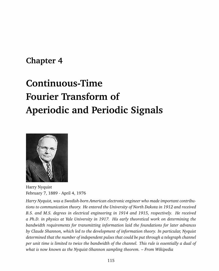
Chapter 4
Continuous-TimeFourier Transform ofAperiodic and Periodic Signals
Harry NyquistFebruary 7, 1889 - April 4, 1976
Harry Nyquist, was a Swedish-born American electronic engineer who made important contribu-tions to communication theory. He entered the University of North Dakota in 1912 and receivedB.S. and M.S. degrees in electrical engineering in 1914 and 1915, respectively. He receiveda Ph.D. in physics at Yale University in 1917. His early theoretical work on determining thebandwidth requirements for transmitting information laid the foundations for later advancesby Claude Shannon, which led to the development of information theory. In particular, Nyquistdetermined that the number of independent pulses that could be put through a telegraph channelper unit time is limited to twice the bandwidth of the channel. This rule is essentially a dual ofwhat is now known as the Nyquist-Shannon sampling theorem. – From Wikipedia
115
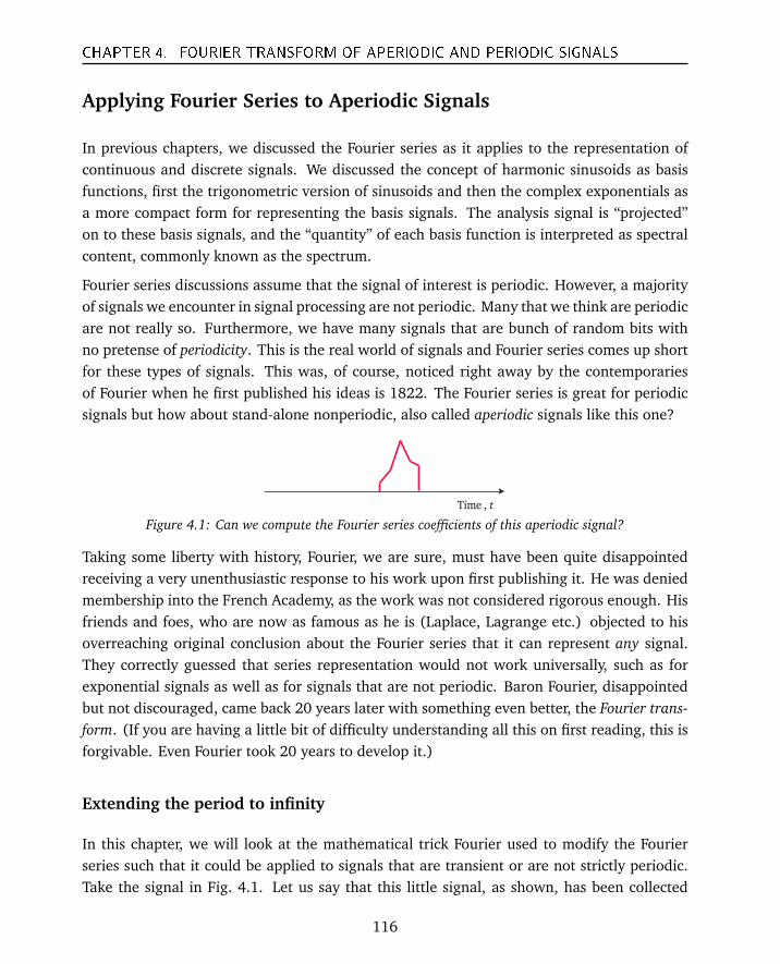
CHAPTER 4. FOURIER TRANSFORM OF APERIODIC AND PERIODIC SIGNALS
Applying Fourier Series to Aperiodic Signals
In previous chapters, we discussed the Fourier series as it applies to the representation ofcontinuous and discrete signals. We discussed the concept of harmonic sinusoids as basisfunctions, first the trigonometric version of sinusoids and then the complex exponentials asa more compact form for representing the basis signals. The analysis signal is “projected”on to these basis signals, and the “quantity” of each basis function is interpreted as spectralcontent, commonly known as the spectrum.
Fourier series discussions assume that the signal of interest is periodic. However, a majorityof signals we encounter in signal processing are not periodic. Many that we think are periodicare not really so. Furthermore, we have many signals that are bunch of random bits withno pretense of periodicity. This is the real world of signals and Fourier series comes up shortfor these types of signals. This was, of course, noticed right away by the contemporariesof Fourier when he first published his ideas is 1822. The Fourier series is great for periodicsignals but how about stand-alone nonperiodic, also called aperiodic signals like this one?
,Time t
Figure 4.1: Can we compute the Fourier series coefficients of this aperiodic signal?
Taking some liberty with history, Fourier, we are sure, must have been quite disappointedreceiving a very unenthusiastic response to his work upon first publishing it. He was deniedmembership into the French Academy, as the work was not considered rigorous enough. Hisfriends and foes, who are now as famous as he is (Laplace, Lagrange etc.) objected to hisoverreaching original conclusion about the Fourier series that it can represent any signal.They correctly guessed that series representation would not work universally, such as forexponential signals as well as for signals that are not periodic. Baron Fourier, disappointedbut not discouraged, came back 20 years later with something even better, the Fourier trans-form. (If you are having a little bit of difficulty understanding all this on first reading, this isforgivable. Even Fourier took 20 years to develop it.)
Extending the period to infinity
In this chapter, we will look at the mathematical trick Fourier used to modify the Fourierseries such that it could be applied to signals that are transient or are not strictly periodic.Take the signal in Fig. 4.1. Let us say that this little signal, as shown, has been collected
116
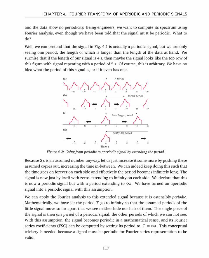
CHAPTER 4. FOURIER TRANSFORM OF APERIODIC AND PERIODIC SIGNALS
and the data show no periodicity. Being engineers, we want to compute its spectrum usingFourier analysis, even though we have been told that the signal must be periodic. What todo?
Well, we can pretend that the signal in Fig. 4.1 is actually a periodic signal, but we are onlyseeing one period, the length of which is longer than the length of the data at hand. Wesurmise that if the length of our signal is 4 s, then maybe the signal looks like the top row ofthis figure with signal repeating with a period of 5 s. Of course, this is arbitrary. We have noidea what the period of this signal is, or if it even has one.
−15 −10 −5 0 5 10 15 20
−15 −10 −5 0 5 10 15 20
Period
Bigger period
Even bigger period
Really big period
Time, t
−15 −10 −5 0 5 10 15 20
−15 −10 −5 0 5 10 15 20
(a)
(b)
(c)
(d)
Figure 4.2: Going from periodic to aperiodic signal by extending the period.
Because 5 s is an assumed number anyway, let us just increase it some more by pushing theseassumed copies out, increasing the time in-between. We can indeed keep doing this such thatthe time goes on forever on each side and effectively the period becomes infinitely long. Thesignal is now just by itself with zeros extending to infinity on each side. We declare that thisis now a periodic signal but with a period extending to ∞. We have turned an aperiodicsignal into a periodic signal with this assumption.
We can apply the Fourier analysis to this extended signal because it is ostensibly periodic.Mathematically, we have let the period T go to infinity so that the assumed periods of thelittle signal move so far apart that we see neither hide nor hair of them. The single piece ofthe signal is then one period of a periodic signal, the other periods of which we can not see.With this assumption, the signal becomes periodic in a mathematical sense, and its Fourierseries coefficients (FSC) can be computed by setting its period to, T =∞. This conceptualtrickery is needed because a signal must be periodic for Fourier series representation to bevalid.
117
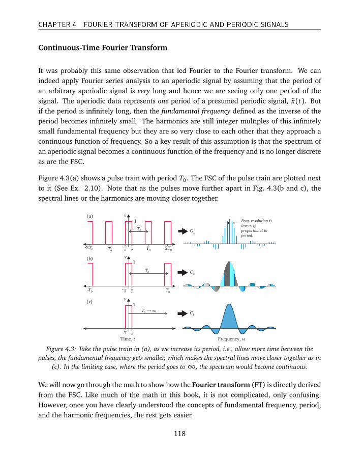
CHAPTER 4. FOURIER TRANSFORM OF APERIODIC AND PERIODIC SIGNALS
Continuous-Time Fourier Transform
It was probably this same observation that led Fourier to the Fourier transform. We canindeed apply Fourier series analysis to an aperiodic signal by assuming that the period ofan arbitrary aperiodic signal is very long and hence we are seeing only one period of thesignal. The aperiodic data represents one period of a presumed periodic signal, x(t). Butif the period is infinitely long, then the fundamental frequency defined as the inverse of theperiod becomes infinitely small. The harmonics are still integer multiples of this infinitelysmall fundamental frequency but they are so very close to each other that they approach acontinuous function of frequency. So a key result of this assumption is that the spectrum ofan aperiodic signal becomes a continuous function of the frequency and is no longer discreteas are the FSC.
Figure 4.3(a) shows a pulse train with period T0. The FSC of the pulse train are plotted nextto it (See Ex. 2.10). Note that as the pulses move further apart in Fig. 4.3(b and c), thespectral lines or the harmonics are moving closer together.
2
τ
2
τ
2
τ
2
τ
2
τ
2
τ
0T
0T
0T0T
0T0T02T
02T
1
1
1
v
v
v
kC
kC
kC
( )a
( )b
( )c
Freq. resolution is
inversely
proportional to
period.
0T →∞
Frequency, ωTime, t
Figure 4.3: Take the pulse train in (a), as we increase its period, i.e., allow more time between thepulses, the fundamental frequency gets smaller, which makes the spectral lines move closer together as in
(c). In the limiting case, where the period goes to∞, the spectrum would become continuous.
We will now go through the math to show how the Fourier transform (FT) is directly derivedfrom the FSC. Like much of the math in this book, it is not complicated, only confusing.However, once you have clearly understood the concepts of fundamental frequency, period,and the harmonic frequencies, the rest gets easier.
118
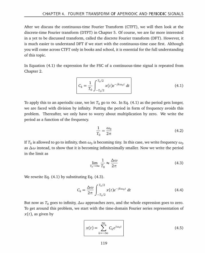
CHAPTER 4. FOURIER TRANSFORM OF APERIODIC AND PERIODIC SIGNALS
After we discuss the continuous-time Fourier Transform (CTFT), we will then look at thediscrete-time Fourier transform (DTFT) in Chapter 5. Of course, we are far more interestedin a yet to be discussed transform, called the discrete Fourier transform (DFT). However, itis much easier to understand DFT if we start with the continuous-time case first. Althoughyou will come across CTFT only in books and school, it is essential for the full understandingof this topic.
In Equation (4.1) the expression for the FSC of a continuous-time signal is repeated fromChapter 2.
Ck =1T0
∫ T0/2
−T0/2
x(t)e− jkω0 t dt (4.1)
To apply this to an aperiodic case, we let T0 go to∞. In Eq. (4.1) as the period gets longer,we are faced with division by infinity. Putting the period in form of frequency avoids thisproblem. Thereafter, we only have to worry about multiplication by zero. We write theperiod as a function of the frequency.
1T0=ω0
2π(4.2)
If T0 is allowed to go to infinity, thenω0 is becoming tiny. In this case, we write frequencyω0
as ∆ω instead, to show that it is becoming infinitesimally smaller. Now we write the periodin the limit as
limT0→∞
1T0≈∆ω
2π(4.3)
We rewrite Eq. (4.1) by substituting Eq. (4.3).
Ck =∆ω
2π
∫ T0/2
−T0/2
x(t)e− jkω0 t dt (4.4)
But now as T0 goes to infinity, ∆ω approaches zero, and the whole expression goes to zero.To get around this problem, we start with the time-domain Fourier series representation ofx(t), as given by
x(t) =∞∑
k=−∞Cke jω0 t (4.5)
119
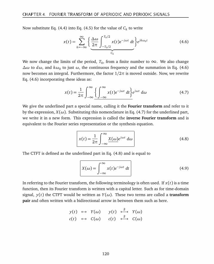
CHAPTER 4. FOURIER TRANSFORM OF APERIODIC AND PERIODIC SIGNALS
Now substitute Eq. (4.4) into Eq. (4.5) for the value of Ck to write
x(t) =∞∑
k=−∞
§
∆ω
2π
∫ T0/2
−T0/2
x(t)e− jωt dt
︸ ︷︷ ︸
Ck
ª
e jkω0 t (4.6)
We now change the limits of the period, T0, from a finite number to ∞. We also change∆ω to dω, and kω0 to just ω, the continuous frequency and the summation in Eq. (4.6)now becomes an integral. Furthermore, the factor 1/2π is moved outside. Now, we rewriteEq. (4.6) incorporating these ideas as:
x(t) =1
2π
∫ ∞
−∞
§
∫ ∞
−∞x(t)e− jωt dt
ª
e jωt dω (4.7)
We give the underlined part a special name, calling it the Fourier transform and refer to itby the expression, X (ω). Substituting this nomenclature in Eq. (4.7) for the underlined part,we write it in a new form. This expression is called the inverse Fourier transform and isequivalent to the Fourier series representation or the synthesis equation.
x(t) =1
2π
∫ ∞
−∞X (ω)e jωt dω (4.8)
The CTFT is defined as the underlined part in Eq. (4.8) and is equal to
X (ω) =
∫ ∞
−∞x(t)e− jωt dt (4.9)
In referring to the Fourier transform, the following terminology is often used. If x(t) is a timefunction, then its Fourier transform is written with a capital letter. Such as for time-domainsignal, y(t) the CTFT would be written as Y (ω). These two terms are called a transformpair and often written with a bidirectional arrow in between them such as here.
y(t) ↔ Y (ω) y(t)F←→ Y (ω)
c(t) ↔ C(ω) c(t)F←→ C(ω)
120

CHAPTER 4. FOURIER TRANSFORM OF APERIODIC AND PERIODIC SIGNALS
The symbol F· is also used to denote the Fourier transform. The symbol F−1· is used todenote the inverse transform such that
Y (ω) = Fy(t)
g(t) = F−1G(ω)
The CTFT is generally a complex function. We can plot the real and the imaginary parts of thetransform, or we can compute and plot the magnitude, referred to as |X (ω)| and the phase,referred to as ∠X (ω). The magnitude is computed by taking the square root of the productX (ω)X ∗(ω) and phase by the arctan of the ratio of the imaginary and the real parts. We canalso write the transform this way, separating out the magnitude and the phase spectrum.
X (ω) = |X (ω)|e j∠X (ω)
Here
• Magnitude Spectrum: |X (ω)|• Phase Spectrum: ∠X (ω).
If the two components of a CE each have an amplitude 1.0 each, then its magnitude is equalto the square-root of 2. The phase of a CE is constant and equal to 0.
Comparing FSC and the Fourier Transform
Continuous
Time (CT)
signals
Discrete
Time (DT)
signals
Fourier Series
Coeffcients
(FSC)
Fourier
Transform
(CTFT)
Fourier Series
Coeffcients
(FSC)
Fourier
Transform
(DTFT)
Periodic Non-periodic Periodic Non-periodic
Fourier Decomposition of Signals
Figure 4.4: Fourier series and the Fourier transform
The Fourier series analysis can be used with both discrete and continuous-time signals as longas they are periodic. When a signal is aperiodic, the premium tool of analysis is the Fouriertransform. Just as the Fourier series can be applied to continuous and discrete signals,the Fourier transform can also be applied to continuous and discrete signals. The discrete
121
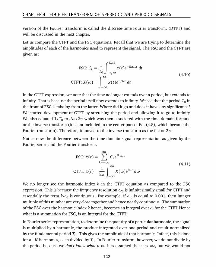
CHAPTER 4. FOURIER TRANSFORM OF APERIODIC AND PERIODIC SIGNALS
version of the Fourier transform is called the discrete-time Fourier transform, (DTFT) andwill be discussed in the next chapter.
Let us compare the CTFT and the FSC equations. Recall that we are trying to determine theamplitudes of each of the harmonics used to represent the signal. The FSC and the CTFT aregiven as:
FSC: Ck =1T0
∫ T0/2
−T0/2
x(t)e− jkω0 t dt
CTFT: X (ω) =
∫ ∞
−∞x(t)e− jωt dt
(4.10)
In the CTFT expression, we note that the time no longer extends over a period, but extends toinfinity. That is because the period itself now extends to infinity. We see that the period T0 inthe front of FSC is missing from the latter. Where did it go and does it have any significance?We started development of CTFT by stretching the period and allowing it to go to infinity.We also equated 1/T0 to dω/2π which was then associated with the time-domain formulaor the inverse transform (it is not included in the center part of Eq. (4.8), which became theFourier transform). Therefore, it moved to the inverse transform as the factor 2π.
Notice now the difference between the time-domain signal representation as given by theFourier series and the Fourier transform.
FSC: x(t) =∞∑
k=−∞Cke jkω0 t
CTFT: x(t) =1
2π
∫ ∞
−∞X (ω)e jωt dω
(4.11)
We no longer see the harmonic index k in the CTFT equation as compared to the FSCexpression. This is because the frequency resolutionω0 is infinitesimally small for CTFT andessentially the term kω0 is continuous. For example, if ω0 is equal to 0.001, then integermultiple of this number are very close together and hence nearly continuous. The summationof the FSC over the harmonic index k hence, becomes an integral overω for the CTFT. Hencewhat is a summation for FSC, is an integral for the CTFT.
In Fourier series representation, to determine the quantity of a particular harmonic, the signalis multiplied by a harmonic, the product integrated over one period and result normalizedby the fundamental period T0. This gives the amplitude of that harmonic. Infact, this is donefor all K harmonics, each divided by T0. In Fourier transform, however, we do not divide bythe period because we don’t know what it is. It is assumed that it is ∞, but we would not
122

CHAPTER 4. FOURIER TRANSFORM OF APERIODIC AND PERIODIC SIGNALS
want to divide by that either. Therefore, we just ignore it, and hence, we are not determiningthe signal’s true amplitude. We are computing a measure of its content but it is not the actualcontent. Moreover, we are missing the same term from all coefficients, hence, the Fouriertransform determines relative amplitudes. Very often, we are only interested in the relativelevels of harmonic signal powers. The Fourier spectrum gives us the relative distribution ofpower among the various harmonic frequencies in the signal. In practice, we often normalizethe maximum power to 0 dB such that the relative levels are consistent among all frequencycomponents.
CTFT of Important Aperiodic Functions
Now, we will take a look at some important aperiodic signals and their transforms, alsocalled transform pairs. In the process, we will use the properties listed in Table 4.1. whichcan be used to compute the Fourier transform of many functions. These properties do notneed proof as they are well known, and we will refer to them as needed for the followingimportant examples. (In most cases, they are easy to prove.) The examples in this sectioncover some fundamental functions that come up both in workplace DSP as well in textbooks,so they are worth understanding and memorizing. We will use the properties listed in Table4.1 to compute the CTFTs in the subsequent examples in this and the following chapters. Allfollowing examples assume that the signal is aperiodic and is specified in continuous-time.The Fourier transform in these examples is referred to as CTFT.
CTFT of an impulse function
Example 4.1.
x(t) = δ(t) (4.12)
This is the most important function in signal processing. The delta function can be considereda continuous (Dirac delta function) or a discrete function (Kronecker delta function), but herewe treat it as a continuous function. We use the CTFT equation, Eq. (4.9) and substitute delta
123
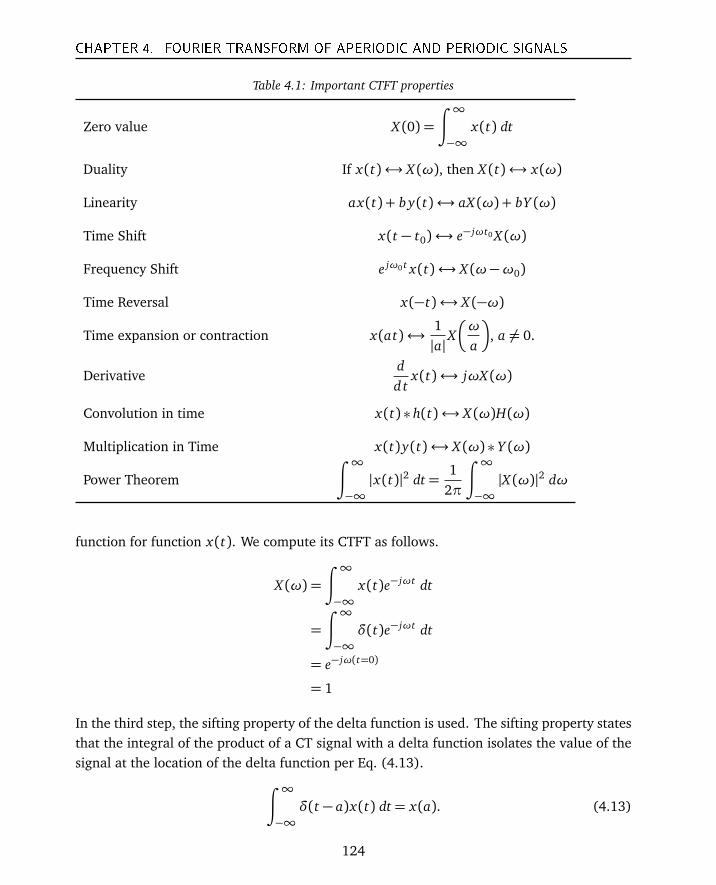
CHAPTER 4. FOURIER TRANSFORM OF APERIODIC AND PERIODIC SIGNALS
Table 4.1: Important CTFT properties
Zero value X (0) =
∫ ∞
−∞x(t) dt
Duality If x(t)↔ X (ω), then X (t)↔ x(ω)
Linearity ax(t) + b y(t)↔ aX (ω) + bY (ω)
Time Shift x(t − t0)↔ e− jωt0 X (ω)
Frequency Shift e jω0 t x(t)↔ X (ω−ω0)
Time Reversal x(−t)↔ X (−ω)
Time expansion or contraction x(at)↔1|a|
X
ω
a
, a 6= 0.
Derivativedd t
x(t)↔ jωX (ω)
Convolution in time x(t) ∗ h(t)↔ X (ω)H(ω)
Multiplication in Time x(t)y(t)↔ X (ω) ∗ Y (ω)
Power Theorem
∫ ∞
−∞|x(t)|2 dt=
12π
∫ ∞
−∞|X (ω)|2 dω
function for function x(t). We compute its CTFT as follows.
X (ω) =
∫ ∞
−∞x(t)e− jωt dt
=
∫ ∞
−∞δ(t)e− jωt dt
= e− jω(t=0)
= 1
In the third step, the sifting property of the delta function is used. The sifting property statesthat the integral of the product of a CT signal with a delta function isolates the value of thesignal at the location of the delta function per Eq. (4.13).
∫ ∞
−∞δ(t − a)x(t) dt= x(a). (4.13)
124
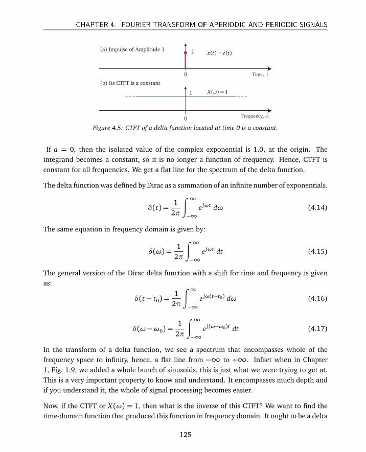
CHAPTER 4. FOURIER TRANSFORM OF APERIODIC AND PERIODIC SIGNALS
t0
0
( ) ( )x t tδ=
( ) 1X ω =
(a) Impulse of Amplitude 1
(b) Its CTFT is a constant
1
1
Time,
Frequency, ω
Figure 4.5: CTFT of a delta function located at time 0 is a constant.
If a = 0, then the isolated value of the complex exponential is 1.0, at the origin. Theintegrand becomes a constant, so it is no longer a function of frequency. Hence, CTFT isconstant for all frequencies. We get a flat line for the spectrum of the delta function.
The delta function was defined by Dirac as a summation of an infinite number of exponentials.
δ(t) =1
2π
∫ ∞
−∞e jωt dω (4.14)
The same equation in frequency domain is given by:
δ(ω) =1
2π
∫ ∞
−∞e jωt dt (4.15)
The general version of the Dirac delta function with a shift for time and frequency is givenas:
δ(t − t0) =1
2π
∫ ∞
−∞e jω(t−t0) dω (4.16)
δ(ω−ω0) =1
2π
∫ ∞
−∞e j(ω−ω0)t dt (4.17)
In the transform of a delta function, we see a spectrum that encompasses whole of thefrequency space to infinity, hence, a flat line from −∞ to +∞. Infact when in Chapter1, Fig. 1.9, we added a whole bunch of sinusoids, this is just what we were trying to get at.This is a very important property to know and understand. It encompasses much depth andif you understand it, the whole of signal processing becomes easier.
Now, if the CTFT or X (ω) = 1, then what is the inverse of this CTFT? We want to find thetime-domain function that produced this function in frequency domain. It ought to be a delta
125
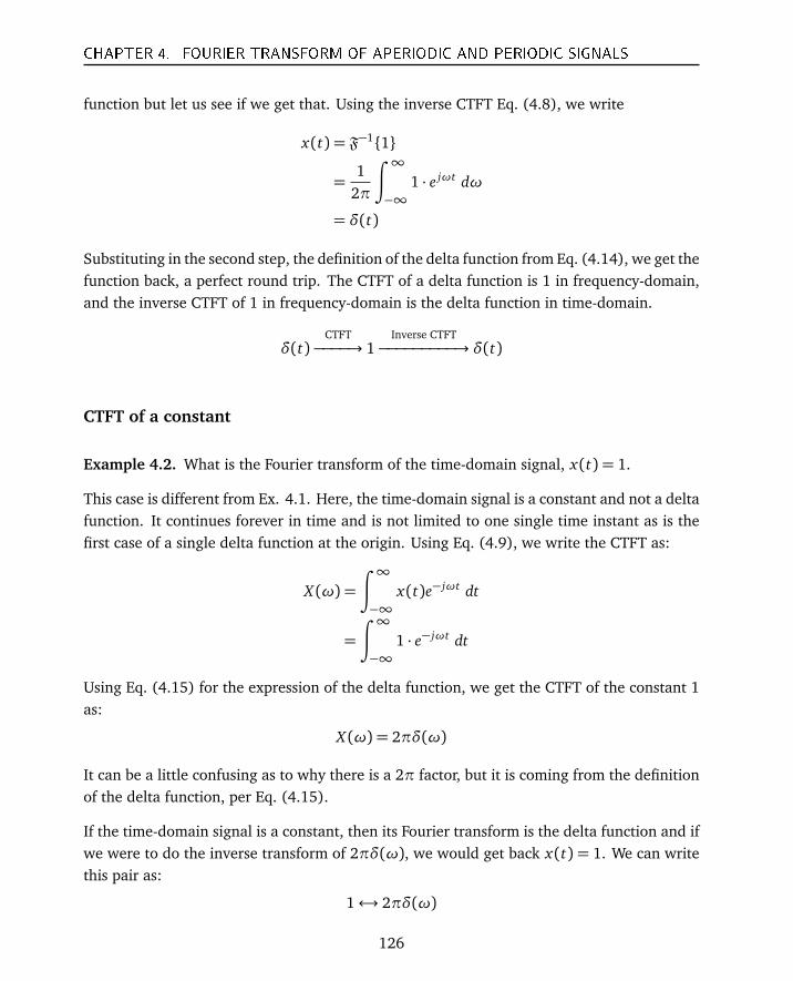
CHAPTER 4. FOURIER TRANSFORM OF APERIODIC AND PERIODIC SIGNALS
function but let us see if we get that. Using the inverse CTFT Eq. (4.8), we write
x(t) = F−11
=1
2π
∫ ∞
−∞1 · e jωt dω
= δ(t)
Substituting in the second step, the definition of the delta function from Eq. (4.14), we get thefunction back, a perfect round trip. The CTFT of a delta function is 1 in frequency-domain,and the inverse CTFT of 1 in frequency-domain is the delta function in time-domain.
δ(t)CTFT−−−−→ 1
Inverse CTFT−−−−−−−−−→ δ(t)
CTFT of a constant
Example 4.2. What is the Fourier transform of the time-domain signal, x(t) = 1.
This case is different from Ex. 4.1. Here, the time-domain signal is a constant and not a deltafunction. It continues forever in time and is not limited to one single time instant as is thefirst case of a single delta function at the origin. Using Eq. (4.9), we write the CTFT as:
X (ω) =
∫ ∞
−∞x(t)e− jωt dt
=
∫ ∞
−∞1 · e− jωt dt
Using Eq. (4.15) for the expression of the delta function, we get the CTFT of the constant 1as:
X (ω) = 2πδ(ω)
It can be a little confusing as to why there is a 2π factor, but it is coming from the definitionof the delta function, per Eq. (4.15).
If the time-domain signal is a constant, then its Fourier transform is the delta function and ifwe were to do the inverse transform of 2πδ(ω), we would get back x(t) = 1. We can writethis pair as:
1↔ 2πδ(ω)
126
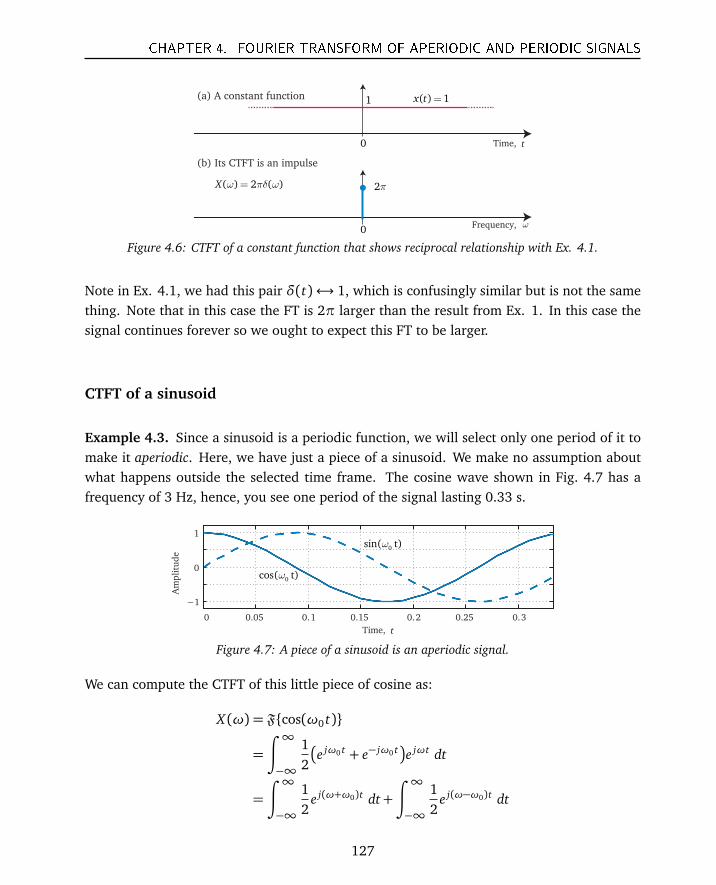
CHAPTER 4. FOURIER TRANSFORM OF APERIODIC AND PERIODIC SIGNALS
1(a) A constant function
(b) Its CTFT is an impulse
( ) 2 ( )X ω πδ ω=
( ) 1x t =
2π
t0 Time,
ω
0Frequency,
Figure 4.6: CTFT of a constant function that shows reciprocal relationship with Ex. 4.1.
Note in Ex. 4.1, we had this pair δ(t)↔ 1, which is confusingly similar but is not the samething. Note that in this case the FT is 2π larger than the result from Ex. 1. In this case thesignal continues forever so we ought to expect this FT to be larger.
CTFT of a sinusoid
Example 4.3. Since a sinusoid is a periodic function, we will select only one period of it tomake it aperiodic. Here, we have just a piece of a sinusoid. We make no assumption aboutwhat happens outside the selected time frame. The cosine wave shown in Fig. 4.7 has afrequency of 3 Hz, hence, you see one period of the signal lasting 0.33 s.
0 0.05 0.1 0.15 0.2 0.25 0.3
−1
0
1
0cos( t)ω
0sin( t)ω
tTime,
Amplitude
Figure 4.7: A piece of a sinusoid is an aperiodic signal.
We can compute the CTFT of this little piece of cosine as:
X (ω) = Fcos(ω0 t)
=
∫ ∞
−∞
12
e jω0 t + e− jω0 t
e jωt dt
=
∫ ∞
−∞
12
e j(ω+ω0)t dt+
∫ ∞
−∞
12
e j(ω−ω0)t dt
127
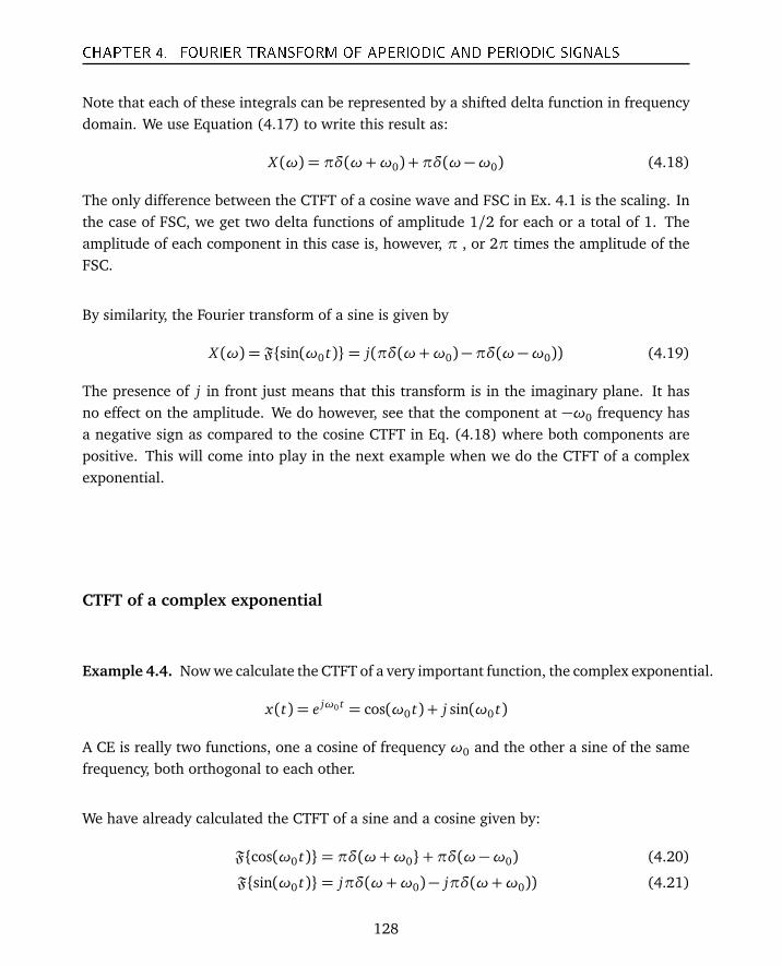
CHAPTER 4. FOURIER TRANSFORM OF APERIODIC AND PERIODIC SIGNALS
Note that each of these integrals can be represented by a shifted delta function in frequencydomain. We use Equation (4.17) to write this result as:
X (ω) = πδ(ω+ω0) +πδ(ω−ω0) (4.18)
The only difference between the CTFT of a cosine wave and FSC in Ex. 4.1 is the scaling. Inthe case of FSC, we get two delta functions of amplitude 1/2 for each or a total of 1. Theamplitude of each component in this case is, however, π , or 2π times the amplitude of theFSC.
By similarity, the Fourier transform of a sine is given by
X (ω) = Fsin(ω0 t)= j(πδ(ω+ω0)−πδ(ω−ω0)) (4.19)
The presence of j in front just means that this transform is in the imaginary plane. It hasno effect on the amplitude. We do however, see that the component at −ω0 frequency hasa negative sign as compared to the cosine CTFT in Eq. (4.18) where both components arepositive. This will come into play in the next example when we do the CTFT of a complexexponential.
CTFT of a complex exponential
Example 4.4. Now we calculate the CTFT of a very important function, the complex exponential.
x(t) = e jω0 t = cos(ω0 t) + j sin(ω0 t)
A CE is really two functions, one a cosine of frequency ω0 and the other a sine of the samefrequency, both orthogonal to each other.
We have already calculated the CTFT of a sine and a cosine given by:
Fcos(ω0 t)= πδ(ω+ω0+πδ(ω−ω0) (4.20)
Fsin(ω0 t)= jπδ(ω+ω0)− jπδ(ω+ω0)) (4.21)
128
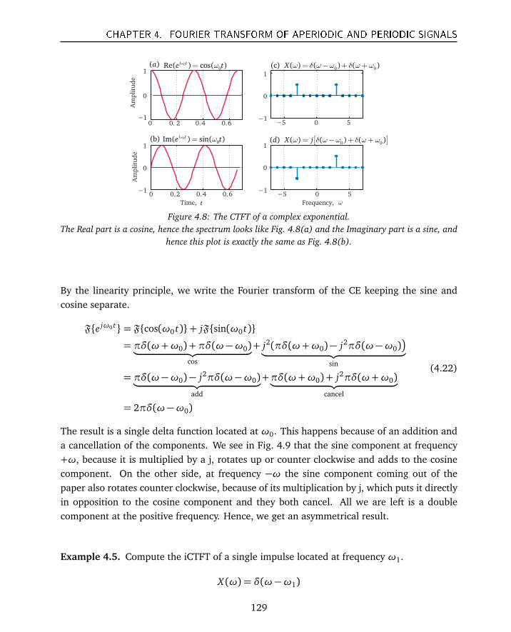
CHAPTER 4. FOURIER TRANSFORM OF APERIODIC AND PERIODIC SIGNALS
0 0. 2 0.4 0.6−1
0
1
Amplitude
−5 0 5−1
0
1
0 0.2 0.4 0.6−1
0
1
Amplitude
−5 0 5−1
0
1
0
0Re( ) cos( )j te t
ω
ω=
0
0Im( ) sin( )j te t
ω
ω=
( )a
(b)
0 0(c) ( ) ( ) ( )X ω δ ω ω δ ω ω= − + +
[ ]0 0( ) ( ) ( ) ( )d X jω δ ω ω δ ω ω= − + +
tTime, ωFrequency,
Figure 4.8: The CTFT of a complex exponential.The Real part is a cosine, hence the spectrum looks like Fig. 4.8(a) and the Imaginary part is a sine, and
hence this plot is exactly the same as Fig. 4.8(b).
By the linearity principle, we write the Fourier transform of the CE keeping the sine andcosine separate.
Fe jω0 t= Fcos(ω0 t)+ jFsin(ω0 t)
= πδ(ω+ω0) +πδ(ω−ω0)︸ ︷︷ ︸
cos
+ j2(πδ(ω+ω0)− j2πδ(ω−ω0)
︸ ︷︷ ︸
sin
= πδ(ω−ω0)− j2πδ(ω−ω0)︸ ︷︷ ︸
add
+πδ(ω+ω0) + j2πδ(ω+ω0)︸ ︷︷ ︸
cancel
= 2πδ(ω−ω0)
(4.22)
The result is a single delta function located at ω0. This happens because of an addition anda cancellation of the components. We see in Fig. 4.9 that the sine component at frequency+ω, because it is multiplied by a j, rotates up or counter clockwise and adds to the cosinecomponent. On the other side, at frequency −ω the sine component coming out of thepaper also rotates counter clockwise, because of its multiplication by j, which puts it directlyin opposition to the cosine component and they both cancel. All we are left is a doublecomponent at the positive frequency. Hence, we get an asymmetrical result.
Example 4.5. Compute the iCTFT of a single impulse located at frequency ω1.
X (ω) = δ(ω−ω1)
129
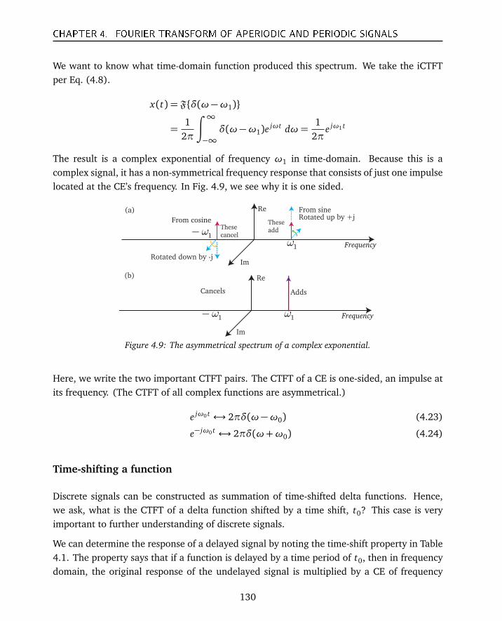
CHAPTER 4. FOURIER TRANSFORM OF APERIODIC AND PERIODIC SIGNALS
We want to know what time-domain function produced this spectrum. We take the iCTFTper Eq. (4.8).
x(t) = Fδ(ω−ω1)
=1
2π
∫ ∞
−∞δ(ω−ω1)e
jωt dω=1
2πe jω1 t
The result is a complex exponential of frequency ω1 in time-domain. Because this is acomplex signal, it has a non-symmetrical frequency response that consists of just one impulselocated at the CE’s frequency. In Fig. 4.9, we see why it is one sided.
Frequency
Rotated up by +j
Rotated down by -j
From cosine
From sine
1ω−
1ω
Frequency
Cancels Adds
1ω− 1ω
Re
Re
Im
Im
(a)
(b)
These
cancel
These
add
Figure 4.9: The asymmetrical spectrum of a complex exponential.
Here, we write the two important CTFT pairs. The CTFT of a CE is one-sided, an impulse atits frequency. (The CTFT of all complex functions are asymmetrical.)
e jω0 t ↔ 2πδ(ω−ω0) (4.23)
e− jω0 t ↔ 2πδ(ω+ω0) (4.24)
Time-shifting a function
Discrete signals can be constructed as summation of time-shifted delta functions. Hence,we ask, what is the CTFT of a delta function shifted by a time shift, t0? This case is veryimportant to further understanding of discrete signals.
We can determine the response of a delayed signal by noting the time-shift property in Table4.1. The property says that if a function is delayed by a time period of t0, then in frequencydomain, the original response of the undelayed signal is multiplied by a CE of frequency
130
CHAPTER 4. FOURIER TRANSFORM OF APERIODIC AND PERIODIC SIGNALS
e jωt0 . In this signal, time is constant and, hence, this is a frequency-domain signal, withfrequency being the variable.
We write the shifted signal as x(t) = δ(t − t0). Now we calculate the Fourier transform ofthis function from Eq. (4.9) as:
X (ω) =
∫ ∞
−∞x(t)e− jωt dt
=
∫ ∞
−∞δ(t − t0)e
− jωt dt
= e− jωt0
In Ex. 4.1, for a undelayed delta function, the CTFT was computed as 1.0. Here the resultis the exponential due to the delay, hence proving the time-shift property. The CTFT of adelayed delta function is a CE. This CE has the form e− jωt0 and might be confusing. That isbecause we are not used to seeing exponentials in frequency domain.
This is a really simple case so we may ask, what is the effect of delay on an arbitraryCTFT? Delaying a signal does not change its amplitude (the main parameter by which wecharacterize signals.) Its frequency also does not change, but what does change is its phase.If a sine wave is running and we arrive to look at it at time t0 after it has started, we aregoing to see an instantaneous phase at that time that will be different depending on whenwe arrive on the scene. That is all a time shift does. It changes the observed phase (or thestarting point of the wave) of the signal.
Figure 4.10 shows the effect of time-delay. In Fig. 4.10(a), a signal with an arbitrary spectrumcentered at frequency of 2 Hz is shown. The time-domain signal is not shown, only its Fouriertransform. You only need to note its shape and center location on the frequency axis. Nowwe delay this signal by 2 s (we do not know what the signal is, but that does not matter.)and want to see what happens to the spectrum.
In Fig. 4.10(b) we draw the CE e jωt0 with t0 = 2 (both sine and cosine are shown). InFig. 4.10(c), we see the effect of multiplying this CE by the spectrum in Fig. 4.10(a). Themagnitude is unchanged. But when we look at Fig. 4.10(d) we see the phase. Since wedo not know what the previous phase was, no statement can be made about it yet. Nowexamine the second column. In this case, the signal is delayed by 4 seconds. Once again inFig. 4.10(g) we see no change in magnitude but we see that phase in Fig. 4.10(h) has indeedchanged from previous case in Fig. 4.10(d). The phase change is directly related to the delay.
131
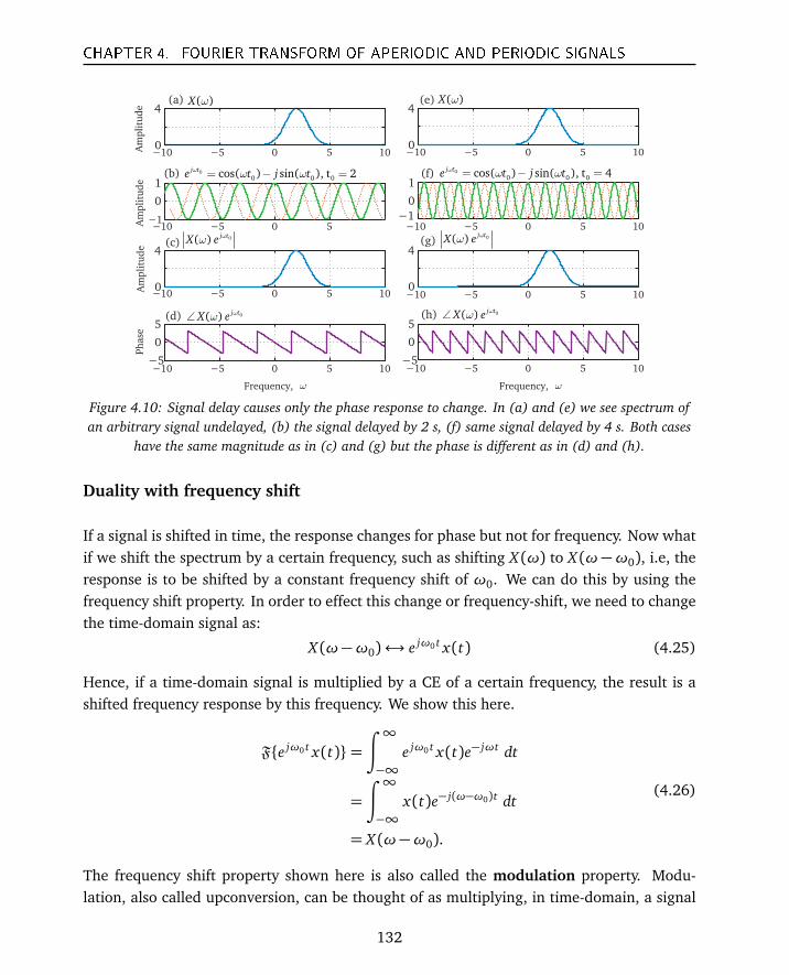
CHAPTER 4. FOURIER TRANSFORM OF APERIODIC AND PERIODIC SIGNALS
−1
0
1
Am
pli
tud
e
−10 −5 0 5 100
4(a)
Am
pli
tud
e
−10 −5 0 5 100
4
Am
pli
tud
e (c)
−10 −5 0 5 10−5
0
5
Ph
ase
(d)
−1
0
1
−10 −5 0 5 100
4
−10 −5 0 5 100
4(g)
−10 −5 0 5 10−5
0
5(h)
(e)
(b) (f)
( )X ω ( )X ω
−10 −5 0 5 10−10 −5 0 5
0
0 0 0cos( ) sin( ), t 2j te t j tω
ω ω= − =
0( ) j tX e
ω
ω0( ) j t
X eω
ω
0
0 0 0cos( ) sin( ), t 4j te t j tω
ω ω= − =
0( ) j tX e
ω
ω∠0( ) j tX e
ω
ω∠
ωFrequency, ωFrequency,
Figure 4.10: Signal delay causes only the phase response to change. In (a) and (e) we see spectrum ofan arbitrary signal undelayed, (b) the signal delayed by 2 s, (f) same signal delayed by 4 s. Both cases
have the same magnitude as in (c) and (g) but the phase is different as in (d) and (h).
Duality with frequency shift
If a signal is shifted in time, the response changes for phase but not for frequency. Now whatif we shift the spectrum by a certain frequency, such as shifting X (ω) to X (ω−ω0), i.e, theresponse is to be shifted by a constant frequency shift of ω0. We can do this by using thefrequency shift property. In order to effect this change or frequency-shift, we need to changethe time-domain signal as:
X (ω−ω0)↔ e jω0 t x(t) (4.25)
Hence, if a time-domain signal is multiplied by a CE of a certain frequency, the result is ashifted frequency response by this frequency. We show this here.
Fe jω0 t x(t)=∫ ∞
−∞e jω0 t x(t)e− jωt dt
=
∫ ∞
−∞x(t)e− j(ω−ω0)t dt
= X (ω−ω0).
(4.26)
The frequency shift property shown here is also called the modulation property. Modu-lation, also called upconversion, can be thought of as multiplying, in time-domain, a signal
132
CHAPTER 4. FOURIER TRANSFORM OF APERIODIC AND PERIODIC SIGNALS
by another single-frequency signal (called a carrier) and infact if you look at Eq. (4.25), thatis exactly what we are doing. A time-domain signal multiplied by a CE, e jω0 t results in thesignal transferring to the frequency of the CE, ω0 without change in its amplitude.
Convolution property
The most important result from the Fourier transform is the convolution property. Infactthe Fourier transform is often used to perform convolution in hardware instead of doingconvolution in time-domain. The convolution property is given by
x(t) ∗ h(t) =
∫ ∞
−∞x(τ)h(t −τ) dτ (4.27)
In time-domain, convolution is a resource-heavy computation. However, convolution can bedone using less computational effort using the Fourier transform. The convolution propertystates:
x(t) ∗ h(t)↔ X (ω)H(ω) (4.28)
This states that the convolution of two signals can be computed by multiplying their individualFourier transforms and then taking the inverse transform of the product. Let us see why thisis possible. We write the time-domain expression for the convolution and then take its Fouriertransform. Yes, it does look messy and requires fancy calculus.
Fx(t) ∗ h(t)= F
∫ ∞
−∞x(τ)h(t −τ) dτ
=
∫ ∞
−∞
∫ ∞
−∞x(τ)h(t −τ)dτe− jωt dt
Now, we interchange the order of integration to get this from
Fx(t) ∗ h(t)=∫ ∞
−∞x(τ)
∫ ∞
−∞h(t −τ)e− jωt dt
dτ
We make a variable change by setting u= t −τ, hence we get
Fx(t) ∗ h(t)=∫ ∞
−∞x(τ)
∫ ∞
−∞h(u)e− jω(u+τ)du
dτ
133
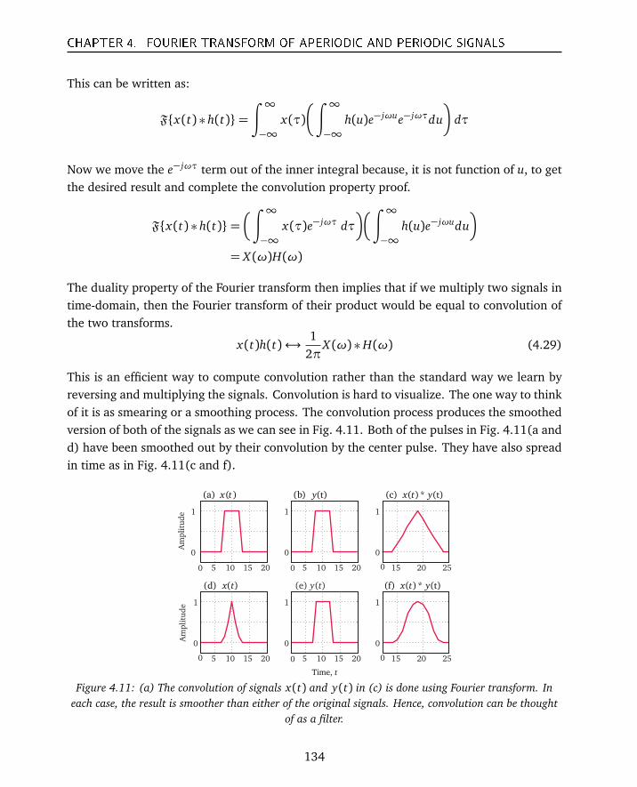
CHAPTER 4. FOURIER TRANSFORM OF APERIODIC AND PERIODIC SIGNALS
This can be written as:
Fx(t) ∗ h(t)=∫ ∞
−∞x(τ)
∫ ∞
−∞h(u)e− jωue− jωτdu
dτ
Now we move the e− jωτ term out of the inner integral because, it is not function of u, to getthe desired result and complete the convolution property proof.
Fx(t) ∗ h(t)=
∫ ∞
−∞x(τ)e− jωτ dτ
∫ ∞
−∞h(u)e− jωudu
= X (ω)H(ω)
The duality property of the Fourier transform then implies that if we multiply two signals intime-domain, then the Fourier transform of their product would be equal to convolution ofthe two transforms.
x(t)h(t)↔1
2πX (ω) ∗H(ω) (4.29)
This is an efficient way to compute convolution rather than the standard way we learn byreversing and multiplying the signals. Convolution is hard to visualize. The one way to thinkof it is as smearing or a smoothing process. The convolution process produces the smoothedversion of both of the signals as we can see in Fig. 4.11. Both of the pulses in Fig. 4.11(a andd) have been smoothed out by their convolution by the center pulse. They have also spreadin time as in Fig. 4.11(c and f).
5 10 15 20
0
1
Am
pli
tud
e
5 10 15 20
0
1
15 20 25
0
1
5 10 15 20
0
1
Am
pli
tud
e
5 10 15 20
0
1
15 20 25
0
1
( ) (t)b y (c) ( )* (t)x t y
(f) ( )* (t)x t y( ) ( )d x t
Time, t
0
00
0
0
0
(a) ( )x t
(e) y(t)
Figure 4.11: (a) The convolution of signals x(t) and y(t) in (c) is done using Fourier transform. Ineach case, the result is smoother than either of the original signals. Hence, convolution can be thought
of as a filter.
134
CHAPTER 4. FOURIER TRANSFORM OF APERIODIC AND PERIODIC SIGNALS
CTFT of a Gaussian function
Example 4.6. Now we examine the CTFT of a really unique and useful function, the Gaussian.The zero-mean Gaussian function is given by
x(t) =1
σp
2πe−t2/(2σ2) (4.30)
where σ2 is the signal variance and σ the standard deviation of the signal. This form of theGaussian is particular to signal processing. A general Gaussian signal is often written in thisform.
f (t) = ae−(t−b)2/2c2(4.31)
Here a is the peak height of the familiar bell curve, b is the center point of the curve and cis the standard deviation.
The CTFT of the Gaussian function is very similar to the function itself.
X (ω) =
∫ ∞
−∞
1
σp
2πe−t2/(2σ2)e− jωt dt
=1
2σp
2π
∫ ∞
−∞e−t2/2σ2
e− jωt dt
This is a difficult integral to solve but fortunately smart people have already done it for us.The result is
X (ω) =1
2σp
2πe−
σ2ω22 (4.32)
As σ is a constant, the shape of this curve is a function of the square of the frequency, sameas it is in time-domain where it is square of time. Hence, it is often said that the CTFT ofthe Gaussian function is same as itself, but what they really mean is that the shape is thesame. This property of the Gaussian function is very important in nearly all fields. However,as we see in Eq. (4.32), there is no hard cutoff in the response and hence the bandwidthof this signal is not finite. How fast it decays depends on the parameter, σ, the standarddeviation. If the x-axis is normalized by the standard deviation, the response becomes thenormal distribution. In signal processing, we find that often noise can be modeled as aGaussian process. We also find that when Gaussian signals are added or convolved, theirjoint distribution retains its Gaussian distribution.
135
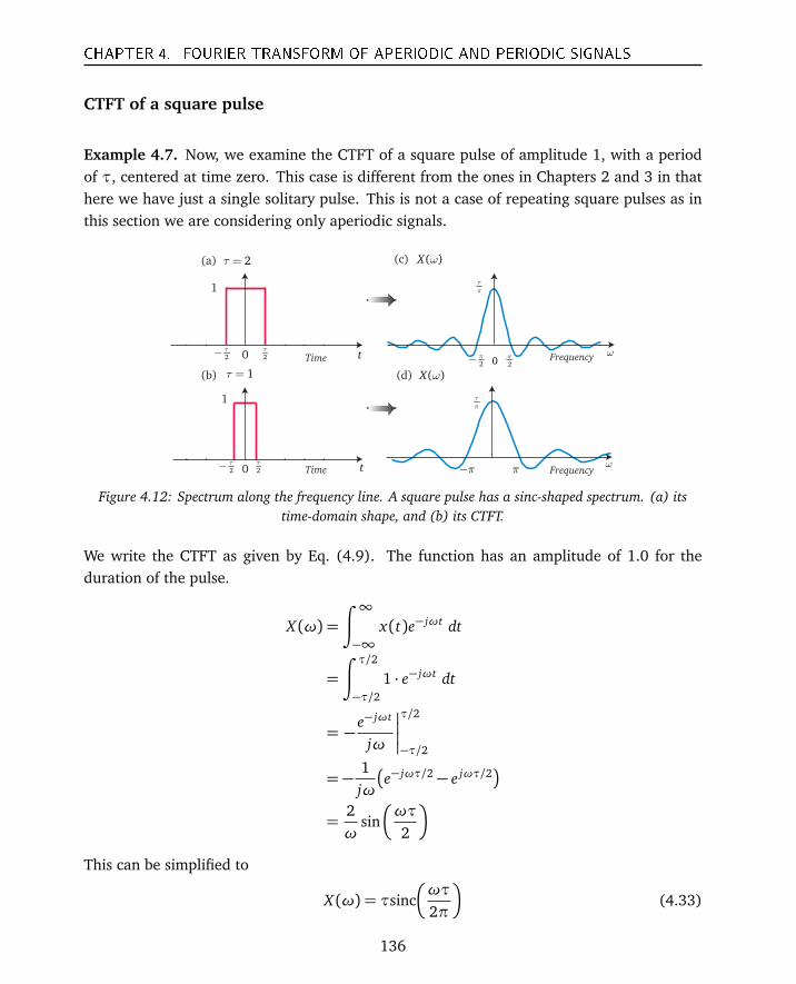
CHAPTER 4. FOURIER TRANSFORM OF APERIODIC AND PERIODIC SIGNALS
CTFT of a square pulse
Example 4.7. Now, we examine the CTFT of a square pulse of amplitude 1, with a periodof τ, centered at time zero. This case is different from the ones in Chapters 2 and 3 in thathere we have just a single solitary pulse. This is not a case of repeating square pulses as inthis section we are considering only aperiodic signals.
0
1
ω2
τ
0
τ
π
(a)
0
1
ω
2
τ
−
2
τ
2
τ
−
2
π
2
π
−
π− π
τ
π
2τ =
(b) 1τ =
(c) ( )X ω
(d) ( )X ω
t
t
Time
Time Frequency
Frequency
Figure 4.12: Spectrum along the frequency line. A square pulse has a sinc-shaped spectrum. (a) itstime-domain shape, and (b) its CTFT.
We write the CTFT as given by Eq. (4.9). The function has an amplitude of 1.0 for theduration of the pulse.
X (ω) =
∫ ∞
−∞x(t)e− jωt dt
=
∫ τ/2
−τ/21 · e− jωt dt
= −e− jωt
jω
τ/2
−τ/2
= −1jω
e− jωτ/2 − e jωτ/2
=2ω
sin
ωτ
2
This can be simplified to
X (ω) = τsinc
ωτ
2π
(4.33)
136
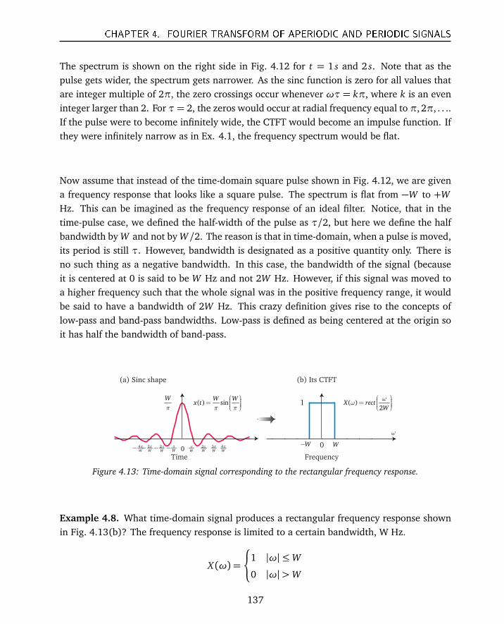
CHAPTER 4. FOURIER TRANSFORM OF APERIODIC AND PERIODIC SIGNALS
The spectrum is shown on the right side in Fig. 4.12 for t = 1 s and 2 s. Note that as thepulse gets wider, the spectrum gets narrower. As the sinc function is zero for all values thatare integer multiple of 2π, the zero crossings occur whenever ωτ = kπ, where k is an eveninteger larger than 2. For τ= 2, the zeros would occur at radial frequency equal to π, 2π, . . ..If the pulse were to become infinitely wide, the CTFT would become an impulse function. Ifthey were infinitely narrow as in Ex. 4.1, the frequency spectrum would be flat.
Now assume that instead of the time-domain square pulse shown in Fig. 4.12, we are givena frequency response that looks like a square pulse. The spectrum is flat from −W to +WHz. This can be imagined as the frequency response of an ideal filter. Notice, that in thetime-pulse case, we defined the half-width of the pulse as τ/2, but here we define the halfbandwidth by W and not by W/2. The reason is that in time-domain, when a pulse is moved,its period is still τ. However, bandwidth is designated as a positive quantity only. There isno such thing as a negative bandwidth. In this case, the bandwidth of the signal (becauseit is centered at 0 is said to be W Hz and not 2W Hz. However, if this signal was moved toa higher frequency such that the whole signal was in the positive frequency range, it wouldbe said to have a bandwidth of 2W Hz. This crazy definition gives rise to the concepts oflow-pass and band-pass bandwidths. Low-pass is defined as being centered at the origin soit has half the bandwidth of band-pass.
0
1 ( )2
X rectW
ω
ω
=
ω
W
π
W
π− 0
( ) sinW W
x tπ π
=
WW−
W
π
(a) Sinc shape
2W
π 3W
π3W
π− 2W
π−4W
π− 4W
π
(b) Its CTFT
Time Frequency
Figure 4.13: Time-domain signal corresponding to the rectangular frequency response.
Example 4.8. What time-domain signal produces a rectangular frequency response shownin Fig. 4.13(b)? The frequency response is limited to a certain bandwidth, W Hz.
X (ω) =
(
1 |ω| ≤W
0 |ω|>W
137
CHAPTER 4. FOURIER TRANSFORM OF APERIODIC AND PERIODIC SIGNALS
We compute the time-domain signal by the inverse CTFT equation.
x(t) =1
2π
∫ ∞
−∞X (ω)e jωt dω
=1
2π
∫ ∞
−∞1 · e jωt dω
=1
2πe jωt
j t
W
−W
Which can be simplified to
x(t) =Wπ
sinc
W tπ
(4.34)
Again we get a sinc function, but now in time-domain. This is the duality principle at work.This is a very interesting case and of fundamental importance in communications.
The frequency spectrum shown in Fig. 4.13(b) is, of course, a very desirable frequencyresponse. We want the frequency response to be tightly constrained. The way to get thistype of spectrum is to use a time-domain signal that has a sinc pulses. But a sinc functionlooks strange as a time-domain signal because it is of infinite length. However, becauseit is “well-behaved,” which means it crosses zeros at predicable points, we can use it as asignal shape, at least in theory. In practice, it is impossible to build a signal shape of infinitetime duration. It has to be truncated, however, truncation causes distortion and we do notget the perfect brick-wall frequency response. An alternate shape with similar properties isthe raised cosine, most commonly used signal shape in communications. The raised cosineshape is also truncated to shorten its length but its distortion is manageable because it decaysfaster than a sinc shape.
In Fig. 4.14 some important Fourier transforms of aperiodic signals are given. A good engineershould know all of these by heart.
Fourier Transform of Periodic Signals
The Fourier transform came about so that the Fourier series could be made rigorously appli-cable to aperiodic signals. The signals we examined so far in this chapter are all aperiodic,even the cosine wave, which we limited to one period. Can we use the CTFT for a periodicsignal? Our intuition says that this should be the same as the Fourier series. Let us see if thatis the case.
138
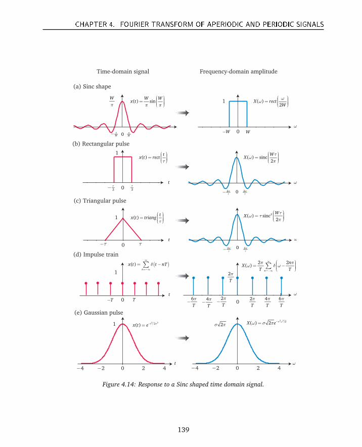
CHAPTER 4. FOURIER TRANSFORM OF APERIODIC AND PERIODIC SIGNALS
0
1 ( )2
X rectW
ω
ω
=
ω
Wπ
Wπ− 0
( ) sinW W
x tπ π
=
0
1
0
( )t
x t rectτ
=
2πτ
2πτ
−
WW−
0
1
−
2τ
2τ−
ττ
t
t
0 2πτ
2πτ
−
( ) sinc2
WX
τ
ω
π
=
2( ) sinc2
WX
τ
ω τ
π
= ( )t
x t triangτ
=
0
1
t
0
t
( )( )n
x t t nTδ
∞
=−∞
= −∑
TT− 2
T
π 4
T
π 6
T
π6
T
π
−4
T
π
−2
T
π
−
2 2( )
n
nX
T T
π π
ω δ ω
∞
=−∞
= − ∑
−4 −2 0 2 4
1
−4 −2 0 2 4
2 2 2( ) 2X eσ ω
ω σ π−=2 22( ) t
x t eσ−= 2σ π
2
T
π
W
π
Time-domain signal Frequency-domain amplitude
(a) Sinc shape
(b) Rectangular pulse
(c) Triangular pulse
(d) Impulse train
(e) Gaussian pulse
t
ω
ω
ω
ω
Figure 4.14: Response to a Sinc shaped time domain signal.
139
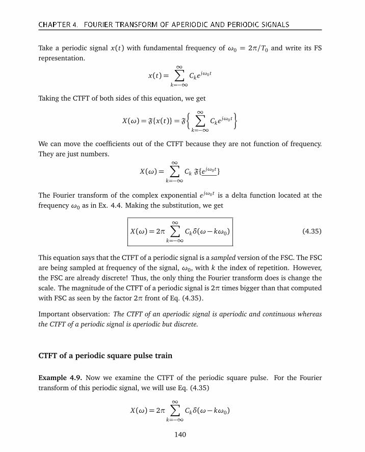
CHAPTER 4. FOURIER TRANSFORM OF APERIODIC AND PERIODIC SIGNALS
Take a periodic signal x(t) with fundamental frequency of ω0 = 2π/T0 and write its FSrepresentation.
x(t) =∞∑
k=−∞Cke jω0 t
Taking the CTFT of both sides of this equation, we get
X (ω) = Fx(t)= F
§ ∞∑
k=−∞Cke jω0 t
ª
We can move the coefficients out of the CTFT because they are not function of frequency.They are just numbers.
X (ω) =∞∑
k=−∞Ck Fe jω0 t
The Fourier transform of the complex exponential e jω0 t is a delta function located at thefrequency ω0 as in Ex. 4.4. Making the substitution, we get
X (ω) = 2π∞∑
k=−∞Ckδ(ω− kω0) (4.35)
This equation says that the CTFT of a periodic signal is a sampled version of the FSC. The FSCare being sampled at frequency of the signal, ω0, with k the index of repetition. However,the FSC are already discrete! Thus, the only thing the Fourier transform does is change thescale. The magnitude of the CTFT of a periodic signal is 2π times bigger than that computedwith FSC as seen by the factor 2π front of Eq. (4.35).
Important observation: The CTFT of an aperiodic signal is aperiodic and continuous whereasthe CTFT of a periodic signal is aperiodic but discrete.
CTFT of a periodic square pulse train
Example 4.9. Now we examine the CTFT of the periodic square pulse. For the Fouriertransform of this periodic signal, we will use Eq. (4.35)
X (ω) = 2π∞∑
k=−∞Ckδ(ω− kω0)
140

CHAPTER 4. FOURIER TRANSFORM OF APERIODIC AND PERIODIC SIGNALS
The FSC of a periodic pulse train with duty cycle= 1/2 are computed in Chapter 2 and givenas
Ck =12
sinc(kπ/2)
−10 −8 −6 −4 −2 0 2 4 6 8 10
0
2
42( )e j
Xωτ
ω−
Frequency
−10 −8 −6 −4 −2 0 2 4 6 8 10−0.2
0
0.2
0.4
kC(a) Fourier series coeff.
(b) CTFT
0T
0T 02T 03T0-2T0-3T
A
0T2τ
2τ
−
Figure 4.15: The periodic square wave with duty cycle of 0.5. (b) Its FSC and (c) its CTFT. Only thescale is different.
We plot these FSC in Fig. 4.15(b). To compute CTFT, we set ω0 = 1 and now we write theCTFT expression as:
X (ω) = 2π∞∑
k=−∞Ckδ
ω− k(ω0 = 1)
The result is the sampled version of the FSC scaled by 2π (See Ex. 2.10) which are of coursethemselves discrete.
What if the square pulse was not centered at 0 but shifted some amount. We can computethe CTFT of this periodic function by applying the time-shift property to the CTFT of theunshifted square wave.
This periodic function is same as Fig. 4.15 but is time-shifted. We can write it as:
y(t) = x(t −τ/2)
141
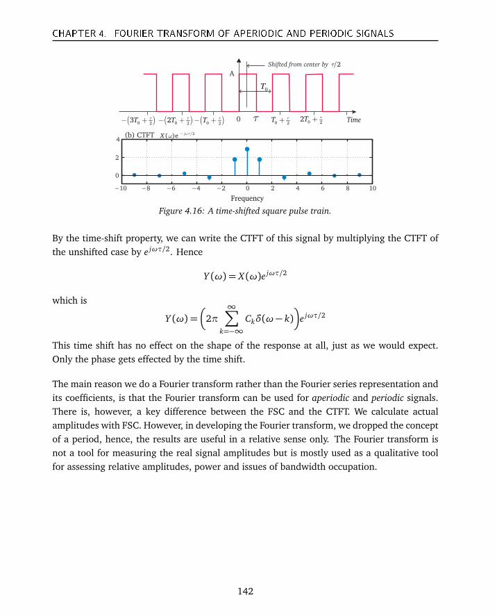
CHAPTER 4. FOURIER TRANSFORM OF APERIODIC AND PERIODIC SIGNALS
0T
A
τ00 2
T τ+ 0 22T τ+( )0 2
2T τ− + ( )0 2T τ− +( )0 2
3T τ− +
Shifted from center by 2τ
Time
−10 −8 −6 −4 −2 0 2 4 6 8 10
0
2
42( )e j
Xωτ
ω−
Frequency
(b) CTFT
Figure 4.16: A time-shifted square pulse train.
By the time-shift property, we can write the CTFT of this signal by multiplying the CTFT ofthe unshifted case by e jωτ/2. Hence
Y (ω) = X (ω)e jωτ/2
which is
Y (ω) =
2π∞∑
k=−∞Ckδ(ω− k)
e jωτ/2
This time shift has no effect on the shape of the response at all, just as we would expect.Only the phase gets effected by the time shift.
The main reason we do a Fourier transform rather than the Fourier series representation andits coefficients, is that the Fourier transform can be used for aperiodic and periodic signals.There is, however, a key difference between the FSC and the CTFT. We calculate actualamplitudes with FSC. However, in developing the Fourier transform, we dropped the conceptof a period, hence, the results are useful in a relative sense only. The Fourier transform isnot a tool for measuring the real signal amplitudes but is mostly used as a qualitative toolfor assessing relative amplitudes, power and issues of bandwidth occupation.
142
CHAPTER 4. FOURIER TRANSFORM OF APERIODIC AND PERIODIC SIGNALS
Summary of Chapter 4
In this Chapter we looked at aperiodic signals and their frequency representations. The FSconcept is extended so that Fourier analysis can be applied to aperiodic signals. In a mannersimilar to computing the coefficients, we call the process of computing the coefficients ofaperiodic signal the Fourier transform. The spectrum of continuous signals using the Fouriertransform is continuous, where the Fourier transform of a periodic signal is discrete.
Terms used in this chapter:
• Fourier Transform, FT• Continuous-time Fourier Transform, CTFT• Discrete-time Fourier Transform, DTFT• Transform pair - The signal in one domain and its Fourier transform in the other
domain are called a Fourier transform pair.
1. Aperiodic signals do not have mathematically valid FSC.2. Fourier transform is developed by assuming that a aperiodic signal is actually periodic
but with an infinitely long period.3. Whereas the spectrum of a periodic signal is represented by the Fourier series coefficients,
the spectrum of an aperiodic signal is called the Fourier transform.4. The term Fourier transform applies not just to aperiodic signals but to periodic signals
as well.5. The FSC are discrete whereas the CTFT of an aperiodic signal is continuous in frequency.6. The CTFT of aperiodic signals is aperiodic.7. The CTFT and the iCTFT are computed by:
CTFT X (ω) =
∫ ∞
−∞x(t)e− jωt dt
iCTFT x(t) =1
2π
∫ ∞
−∞X (ω)e jωt dω
8. A function and its Fourier transform are called a transform pair.
x(t)↔ X (ω)
143
CHAPTER 4. FOURIER TRANSFORM OF APERIODIC AND PERIODIC SIGNALS
9. The CTFT of a periodic signal is given by the expression
X (ω) = 2π∞∑
k=−∞Ckδ(ω− kω0)
10. The CTFT of a periodic signal can be considered a sampled version of the FSC.11. Unlike the CTFT of an aperiodic signal, the CTFT of a periodic signal is discrete, just
as are the FSC for a periodic signals.
Questions
1. What is the conceptual difference between the Fourier series and the Fourier transform?2. Why is the CTFT continuous? Why are the CTFSC coefficients discrete?3. What is the CTFT magnitude of these impulse functions:δ(t − 1) , δ(t − 2) , δ(t − T ).
4. Give the expression for the CTFT of a cosine and a sine. What is the difference betweenthe two?
5. Given a sinusoid of frequency 5 Hz. What does its CTFT look like?6. What is the difference between the Fourier transform magnitude of a sine and a cosine
of equal amplitudes?7. What is the CTFT (amplitude) of these sinusoids: sin(−800πt) , − cos(250πt) , 0.25 sin(25πt).
What is the magnitude spectrum of these sinusoids?8. What is the value of sin(500πt)δ(t), cos(100πt)δ(t −π)?9. What is the CTFT of: x(t) = 6 sin(10πt)− 4cos(4πt)?
10. If the FT of a signal is being multiplied by this CE: e− j6π f , what is the resultant effectin time domain?
11. We multiply a signal in time domain by this CE: e− j12πt , what is the effect in frequencydomain on the FT of the signal?
12. The summation of complex exponentials represents what function?13. What is the value of cos(6πt) ∗δ(t − 4)?14. What is the CTFT of the constant π?15. A sinc function crosses first zero at π/B. What is its time domain equation? What does
the spectrum look like and what is its bandwidth?16. A sinc function crosses first zero at t = 1, give its time domain equation? What does
the spectrum look like and what is its bandwidth?17. What is the CTFT of sin(5πt) ∗δ(t − 5)?
144
CHAPTER 4. FOURIER TRANSFORM OF APERIODIC AND PERIODIC SIGNALS
18. A signal of frequency 4 Hz is delayed by 10 s. By what CE do you multiply the unshiftedCTFT to get the CTFT of the shifted signal?
19. Given x(t) = sinc(tπ), at what times does this function cross zeros?20. The first zero-crossing of a sinc function occurs at time = B s; 0.5 s; 2 s. What is the
bandwidth of each of these three cases?21. What is the main lobe width of the CTFT of square pulses of widths: Ts, Ts/2, π/2,
and 3 s.22. If the main lobe width of a sinc function (one sided) is equal to π/2, then how wide is
the square pulse in time?23. What is the CTFT of an impulse train with period equal to 0.5 s. Is this a periodic
signal?24. Convolution in time domain of two sequences represents what in frequency domain?25. What is the Fourier transform of an impulse of amplitude 2 V in time domain?26. If a signal is shifted by 2 s, what happens to its CTFT?27. The CTFT of a periodic signal is continuous while the CTFSC is discrete. True or false?28. If the CTFSC of a signal at a particular harmonic is equal to 1/2, then what is the value
obtained via CTFT at the same harmonic?29. Given the FSC of a signal, how do you calculate the FT of this signal?30. What is modulation and how is it accomplished?31. Why do the base-band and pass-band bandwidths of a signal differ?
145

CHAPTER 4. FOURIER TRANSFORM OF APERIODIC AND PERIODIC SIGNALS
146
Chapter 5
Discrete-TimeFourier Transform ofAperiodic and Periodic Signals
Paul Adrien Maurice Dirac1902 – 1984
Paul Adrien Maurice Dirac was an English theoretical physicist who made fundamental contri-butions to the early development of both quantum mechanics and quantum electrodynamics. Hewas the Professor of Mathematics at the University of Cambridge, and spent the last decade of hislife at Florida State University. Among his discoveries, he formulated the Dirac equation, whichdescribes the behavior of fermions and predicted the existence of antimatter. Dirac shared theNobel Prize in Physics with Erwin Schrödinger. He also did work that forms the basis of modernattempts to reconcile general relativity with quantum mechanics. Paul Dirac in his influential1930 book The Principles of Quantum Mechanics, introduced the "delta function" which he usedas a continuous analogue of the discrete Kronecker delta. – From Wikipedia
147