the laminar boundary-layer equations, i. motion of...

The laminar boundary-layer equations I. Motion of an elliptic and circular cylinders

B y D. M e k s y n , D.Sc.

{Communicated by G. Temple,F.R.S.—Received 3 June 1947)

The main results obtained are as follows:(a) The problem is reduced, for the front part of a cylinder, to a non-linear differential

equation of the same form as that studied by Falkner & Skan (1930), namely,

r + / r -A d -/'*).This equation has been numerically solved by Hartree (1937), so that the evaluation of

velocities and surface friction requires only very simple and short computations.Near the separation point the problem leads to a more complicated differential equation

(3-20).(b) Elliptic cylinder. The calculated and observed velocities agree up to and including

the point x = 1*457 (§5), where x is the distance along the boundary of the ellipse from the forward stagnation point, expressed as a multiple of the minor axis.

An approximate integration, by neglecting certain terms in the equation (3*20), gives the separation point at about 108° 30' from the stagnation point, as against 103° observed, where the angle corresponds to the elliptic co-ordinate of (4*1).

(c) Circular cylinder. In all cases the calculated surface friction shows good agreement with the observed results, and the results previously obtained from experimental pressure distributions, for the front part of the cylinder.

In the case of the cylinder of diameter d = 5*89 in. the calculated results (by neglecting certain terms in the equation (3*20)) show good agreement with observations almost up to separation point.

(d) Pressure consists of two terms: one is equal to the pressure of the potential flow, the other one depends on the thickness of the boundary layer.

1 . I n t r o d u c t io n

Several methods have been developed for the solution of the laminar boundary- layer problems in two dimensions.

Critical surveys were recently given by Howarth (1934) and Goldstein (1938), and are well known; accordingly, no attempt is made to give here a detailed account of the methods which they discuss, but only to indicate their main trends.

The solution of laminar flow equations is based on Prandtl’s (1904), and Prandtl & Betz (1927) idea of a boundary layer; namely, that the velocity of flow parallel to the surface of a solid body reaches the value corresponding to potential flow, from zero on the surface, through a very thin layer the thickness of which is of order R~*, compared with the dimensions of the body, where R is an appropriate Reynolds number; this enables us to simplify the equations of motion, and the simplified equations were solved by Blasius (1908) and Hiemenz (1911) for the case of an infinitely thin plane lying parallel to the main flow.

Their method of solution could not, however, be applied to other boundaries, because in the case of a plane the pressure gradient vanishes, whereas it appears in the equations of motion for other boundaries.

Vol. IQ2 . A. [ 545 ] 36

on August 26, 2018http://rspa.royalsocietypublishing.org/Downloaded from

http://rspa.royalsocietypublishing.org/

546 D. Meksyn

Accordingly, it was necessary in such cases either to make use of the pressure of the potential flow, or to measure the pressure, or else to assume certain functions for the velocity outside the boundary layer.

The equations were then solved either by expansion in double series, so that the partial differential equations were reduced to a set of ordinary equations (Blasius 1908; Hiemenz 1911; Falkner & Skan 1930; Howarth 1938; Bairstow 1939; or by step-by-step integration (Bairstow 1925; Green 1930; Goldstein 1930).

Karman & Millikan (1934) integrated Mises’s (1927) form of the boundary-layer equations for assumed velocity distributions outside the boundary layer.

Doenhoff (1935) and Millikan (1936) applied Karman’s method to the pressure distribution measured by Schubauer on an elliptic cylinder.

A different line of approach was put forward by Karman (1921); integrating the equations of motion across the boundary layer, Karman obtained the momentum equation.

Assuming simple expression for the velocity across the boundary layer, Polhausen (1921) obtained good approximate solutions.

This method was extended by Dryden (1934) for cases where Polhausen’s method

Thom (1928) suggested the solution of the equations of viscous flow by an iterative process, by dividing the flow into a rectangular net; this method, however, is very laborious.

Piercy, Preston & Whitehead (1938) attempted to solve the equations by successive approximations.

The equations of laminar motion were solved rigorously by Karman (1921) for the case of an infinite rotating disk.

The aim of the present paper is to derive and integrate the equation of the boundary layer in two dimensions, for boundaries which do not have very small radii of curvature, and the potential flow around which is known.

The work consists of two parts. In the first (hydrodynamical) part the general equations of the boundary layer are derived, partly solved for the cases of an elliptic and circular cylinders, and the results obtained compared with Schubauer’s (1935) and Fage & Falkner’s (1931) measurements.

In the second part the mathematical details of the solution are given.

A. EQUATIONS OF STEADY MOTION OF THE BOUNDARY LAYER

2 . S e m i-i n f i n i t e p l a n e c a s e a n d it s g e n e r a l iz a t io n ;THE MATHEMATICAL ANALYSIS

The boundary-layer equation for a semi-infinite plane lying along the main flow, which is in the direction of x positive, is

failed.

32w V\ ?

( 2- 1)



547The laminar boundary-layer equations. I

in the usual notation, the boundary conditions being

u = v = 0 at = 0, = at oo,

where u0 is the velocity at infinity.If we introduce the stream function

d\]fd y ’

djrdx

and new variables cr = y, ft =Jj \ VX J

the equation (2-1) is reduced to an ordinary differential equation

r+fr = o,

( 2-2 )

(2-3)

(2-4)

(2-5)

and the boundary conditions

f = f ' = 0 at cr = 0, / ' = 1 at cr = oo. (2*6)

This equation can be solved by successive approximations (Weyl 1941). As a first approximation, assume

AO) = (2-7)

whence (2*8)

which satisfies the boundary conditions at = 0, Substituting (2*8) in (2-5), and integrating

f = (2-9)

From (2*7) it is obvious that A = a,(2-10)

whence the constant a is found from the condition at infinity (2-6)

/ , ( 0 0 ) = / oae~iaa*d(r = 1. ( 2- 11)

The integral (2-11) can be evaluated in gamma functions, and leads to the value a = 0-684, as against the rigorous value a = 0-664, the difference being about 3 %.

A better approximation can be easily obtained, but it is not needed for our purpose. It is important now to fix the order of magnitude of Since for laminar flow,

assuming that the kinematic viscosity v = 1,

u x length ~ R*, dy (2-12)

it follows from (2-3) thatw * •

(2-13)

whence (2-4) ijr~RK (2-14)3 6 -2



548 D. Meksyn

Consider now laminar motion round a boundary whose inviscid flow is given by the velocity potential a and stream function referred to speed unity at infinity; a and ft have, thus, the dimensions of length, and oc + ift is the complex potential, on the boundary ft = 0.

Assume that the viscous stream function is represented by an expression like

ft~u\I dojI e&<°’ei)A((i),<x)da), (2*15)Jo Jo

where oj = R*fta(awdiere A(oj, a) and a(a) are slowly varying functions, and

f 00

I ego», a)A((o,a)d<o~order unity, (2*16)

and where v is assumed to be unity.The function £(w, a) is, of course, negative for large values of oj, and is such that

e£(«>,a) tends rapidly to zero for moderate values of oj.The assumed form of ft can represent the flow in the boundary layer; in fact,

and at ft = oj = 0,

at ft — oj — oo;

the same holds good for The frictional force is

(2-17)

(2*18)

02

We^M' a)A(oj, a) d<D + R e^0,’a) A (oj, a) j (2-19)

and at ft = 0,

i.e. the velocity and the frictional force have the correct orders of magnitude in such an expression.

Consider now the order of magnitude of the differential coefficients of Since ^ is a slowly varying function of a, the derivatives ... are of

the same order of magnitude as ft.The differential coefficients with respect to ft are of orders

dft d2ftw w

R, R*, (2 -20)

whence the following important conclusion obtains:Laminar motion can be expressed in the space of a and ft (the velocity potential

and the stream function) by a function ft whose second derivative with respect to




ft is a function of a and ft consisting of a slowly varying factor multiplied by an exponential function, rapidly varying with respect to and which tends to zero for very small values of ft.

The derivatives with respect to a preserve the order of magnitude of the function, whereas the derivatives with respect to ft increase the order of the function by R i the order of magnitude of i/r is RK

Let a and ft be the velocity potential and the stream function respectively, corresponding to a given boundary, and the speed unity at infinity, i.e. a and have the dimensions of length.

It is also assumed that on the boundary ft = 0, the curves cl = const, and = const, are orthogonal.

Let the usual Cartesian co-ordinates be x and y, and let

We have now to expand (3-5), and to assess the order of magnitude of the terms; to that end it is necessary to bear in mind that h and its derivatives are slowly varying functions of a and ft of order unity.

3. T he equations op motion

z — x + iy,

(3-1)

the element of length ds in the space of a and ft being

ds2 = p ( da2 + 2). (3-2)

The equation of motion, in the usual notation, is

where (hft _ dxjf '

(3-3)

where is the stream function of the viscous flow.Transforming £ (3*3) to the new co-ordinates* a and ft, we obtain

(3-4)

whence the equation of motion becomes

(3-5)

* The transformation to the a and ft co-ordinates was previously used by Piercy et al. (1938).



Now \Js (2-14) is of order Ri ;hence the equation (3-5) becomes (3*4):

550 D. Meksyn

wR Ri Ri

R 2

(3-6)

where the order of magnitude of the terms is indicated underneath (it is assumed that v = 1).

It we retain the terms of orders R4 and we find that

dxjr d2ifr_r _ rSlog h2d\]fd2x / f logd/3 da d/32 0a dfi d/32 da d/3z \_da d/32 d/3 J

where terms in the square brackets are of order R2. Now when log A2 is expanded in powers of /3,

d log 2

r a i o g & w is >0/?4

/Slog A2\ /02logA2\[ da ) 0+ \d a d /3 ) / ’

(3-7)

(3-8)

where the expressions in the brackets are taken for /? From (3’7) and (3*8)

S r s^ d2\Jf dx/rd2\Jf+d/3\_d/3 dad/3 0a

l /d lo g h 2\ / 0 f \ 2~| /02log^2\ d f d 2r/r log2 [ d a : 0\d/3) y \ dad/3 ) 0d/3d/32Pdad/32 d/3

0 V 0 logVd/3* + 2v d/3 d/32' (3-9)

We now integrate (3*9) with respect to /? from oo to /3, and rearrange the terms, obtaining

d3r/r d\Jf d2\]r dx/rd2 1/0 logm - * ]d/P d fid a d fi da 3/jf2 2 \ da

_ /3 io g ^ \ dhjr p r / a2iog/t2\ d id * * / s i o g » a w i „ . iml W j„3^+J„U tedfi Ivd/ld/pP \ dfi ) 0d a d / p ] d/)- (3K)

9 = P at / » - « . (3-11)

The second and third derivatives of xjr vanish at infinity; on the right-hand side of (3-10) all the terms are of lower order, therefore the values of (0log&2/0/?)... are taken at /3 — 0.

where



The laminar boundary-layer equations. I 551

The equation (3*10) can be considerably simplified, and transformed partly into an ordinary differential equation, as follows. y

Put l + a = y, (3-12)

where lis a length such that at the stagnation point

l + a = y = 0. \ (3-13)

It is also assumed that the velocity of the main flow is in the direction of x positive, and is equal to u0 at infinity.

Now, in the usual Cartesian co-ordinates,

but at infinity

d\jf _ d\Jr da drjr dy da dy dy’

whence

Introducing new variables

drjr¥1 I2u2 ( it'f ) ‘A

at /3 = oo.

\Jr = (2 vu0y)lf(o

we obtain di/f_ df d2\Jf_ uQ (2uoy d3i/r dzf= dfp = J \ T y ) Jo5 ’ W =

d f 1 / 2 « 0\W df d}\

dad/3 2 yda2 0 da d y ‘

(3-14)

(3-15)

(3-16)

(3-17)

(3-18)

From (3*11) and (3-18)

whence q = u0, and

dr/r¥= 1 , at da

at /? = oo,

00. (3-19)

If we substitute (3-18) in (3-10), and make use of (3-19), the general equation of motion of the boundary layer is obtained, namely,

03/0O-3

+ M +2j p v ^ i j ^ \ r ( / ) 2- 1]da2 J_0y0cr2 dadadyj \ da J0 [_\da/ J

i swhere the order of magnitude of the terms appears explicitly.



Since the velocity vanishes on the boundary, i.e. at = cr = 0, the function /(er,y) satisfies the following conditions (3-19):

f = S— = 0 at er = 0, = 1 at (3*21)cor

For the front part of the cylinder the equation (3*20) can be simplified and takes the form

f " + //’ = - r ^ l r - 2) <> - / '2> = A(* -Z'2)’ <3’22)

where the differentiations are taken with respect to cr, and A is introduced for brevity.This has the same form as the well-known equation, of Falkner & Skan (1930).

It was numerically integrated by Hartree (1937). An abridged table of Hartree’s results is given at the end of the paper in table 4; its analytical solution is discussed in the next paper.

552 D. Meksyn

B. ELLIPTIC CYLINDER

4. General formulae

We now introduce the usual elliptic co-ordinates

x = c cosh £ cos rj, sinh £ sinz = x + iy — ccosh (£ = c cosh £,

where £ should not be confused with vorticity.Consider the flow round an ellipse corresponding to £ = £0, the major axis being

directed parallel to the main flow which is in the direction of x positive, the velocity at infinity being u0.

For this case

(4-1)

whence

oc = ce$0 cosh (£ — £0) cos y, /? = ce « sinh (£ — £0) sin y,

W = a, + i/3 = ce o cosh (£ — £0 + iy), ^dW _ dz

h2=

dW d£ = r sinh (£ -£ 0) d£ dz sinh £ *

dW 2 _ ^ cosh 2(£ — £0) — cos 2y dz cosh 2£ — cos 2y

(4-2)

(4-3)

We have now to evaluate the differential coefficients of log h2 with respect to a and /?; to that end the differential coefficients of £ and y have to be found with respect to a and /?.

On differentiating (4-2) we find that

doc = ce^ofsinh (£ — £0) cos iyd£— cosh (£ — £0) sind/? = ce£»[cosh (£ — £0) sin ?/d£ + sinh (£ — £0) j



From these results it is easily found that

0£ _ sinh (g -g 0)cos 9/ 0£ cosh (g - g0) sin 9/da A ’ 0 / ? A09/ cosh (£ — £0) sin 9/ 09/ _ sinh (£ — £0) cos 9/ -_ = , p - A“ ’

A = ce^»[sinh2 (£ — £0) cos2 9/ + cosh2 (£ — £0) sin2 9/]. .

We now introduce the new co-ordinates y (3-12),

y = ce » + a = ce «[l + cosh (£ - £0) cos 9/],


(4-5)

(4-6)

where, as assumed, y vanishes at the stagnation point

£ = £o>

On differentiating log A2 (4-3) it is found, after few transformations, that

cosh 2£0 — 1 cos 9/ cosh 2£0 — cos 29/ sin2 £9/ ’

2 sinh 2£0 cosh 2£0 — cos 29/ cot £9/,

[cosh 2£0 —1 + 6 sin2 9/] sinh 2£0 cos 9/ cos £9/ (cosh 2£0 — cos 2 9/)2 sin3 9/ ’

(4-7)

the above expressions being evaluated for 0, i.e. on the boundary.For the front part of the cylinder the simplified equation (3-22) will be considered,

and it will be shown below that it leads to results in complete agreement with observations.

The equation (3*20), where the terms containing partial differential coefficients with respect to y are disregarded, will be considered for the motion near the separation point.

5. E xperimental results. P reliminary formulae

Extensive measurements were carried out by Schubauer (1935) on a flow round an elliptic cylinder, the major and minor axes of the ellipse being

2 a = 11-78 in., 26 = 3-98 in. (5-1)respectively.

The cylinder was placed in a wind tunnel with the major axis of the ellipse along the main flow, the velocity of the main stream being about w0 = l l -5ft./sec.

The pressure on the boundary and the velocity u parallel and close to the boundary were measured at many points before and after separation.

The co-ordinate x was measured along the boundary, starting from the forward stagnation point, and the distance, expressed as a multiple of the minor axis, was denoted by x; the co-ordinate y is taken normal to the boundary.



554

The angles r] (4-1) corresponding to the at the measured points are given in table 1, where only data needed below are included. The angular distance from the forward stagnation point is equal to n — rj; separation was observed at = 1*99, i.e. at 103° 10' from stagnation point.

D. Meksyn

T a b l e 1

x 0 0-180 1-097 1-457 1-832 1-99y n 161° 32' 111° 59' 97° 36' 83° 6' 76° 50'

The connexion will now be found between Schubauer’s length x and our units expressed in the space of a, /?.

The expressions to be considered are

1 (2u0y\*fi }z \ v ) y ’

ot = ce£° cosh (£ — £0) cos rj, ft = ce o sinh (£ - £0) sin tj, y = ce£«[ 1 + cosh (£ — £0) cos

(5-2)

It is important, in what follows, to distinguish between different systems of co-ordinates; three of them are used in the present analysis:

(i) the ordinary Cartesian co-ordinates x, y (not to be confused with Schubauer’s);(ii) elliptic co-ordinates £, y, where

x = ccosh£ cosi/, = csinh£ sim/; (5-3)

(iii) the co-ordinates a, /? (5-2) which can be termed the ‘potential co-ordinates’. Lengths in different systems of co-ordinates are connected by the rule that an

element of length ds is invariant with respect to transformations of co-ordinates; whence for the case of Cartesian and elliptic co-ordinates

ds2 = dx2 + d y 2 = ^ (d ^ + drj2)rtx1 c2 (5-4)2 = ^ (cosh 2£-cos2V),

and the components of the velocity parallel and normal to the ellipse are respectively

dx/rAjgg-, Mj - h W'Sr,' (S-5)

Below only the velocity u will be required, whence

dfi d\/r 1 d/3

/ cosh 2£0 — cos 2 y \-i dfsin?/. (5-6)




Since the thickness of the boundary layer is very small, it was assumed in the above that across the boundary layer £ = £0, and the expression (5-6) was simplified accordingly.

We have to find, in what follows, the velocity uv in the boundary layer at a point 7) — const, as a function of its normal distance from the boundary; from (5-2)

since y = ce^(l +cosrj) remains constant, and (5*2)A/? = ce o cosh (£ — £0) sin A£ S sin rj. A£.

Since an element of length in elliptic co-ordinates isc2 ds2 = — (cosh 2£ — cos 2 + drj2),

an element of length dn along a normal to the ellipse (rj = const.) is

dn ^ cosh 2£0 — cos 2i/j»

whence combining (5-7), (5-8), (5*10) and from (5-6) it is finally obtained: 1 / 2w0\ * / cosh 2£0 — cos - i ^

- m u

u0 \

-J e£° sin 7] An = q An,

cosh 2£0 — cos 2rj\-l df , .— 2----------I

where q is introduced for brevity.Schubauer expressed lengths in terms of

2 b ’yRl

(S-7)

(5-8)

(5-9)

(5-10)

(5-11)

(5-12)

where yn is taken normal to the boundary, and measured in the usual units of length.It is clear that Vn = Arc, (5-13)

whenceA ct 2bq

(5-14)

which gives the connexion between our variable Act and Schubauer’s length

6 . T h e v e l o c it y i n t h e b o u n d a r y l a y e r . F r o n t p a r t

A comparison will now be made between the calculated velocities in the boundary layer, and those measured by Schubauer.

From the stagnation point up to 70 % to the separation point the simplified equation (3-22)

(6*1)r + f

tdlogh2]= A ( l - / '2),

k [cosh 2£0 — 1] cos rj |l 9a J'0 [cosh 2£0 — cos 2 sin2 \ tj ’J



556

holds good, i.e. the influence of the disregarded terms is unimportant; that corresponds to Schubauer’s measurements up to

x —1-457, i.e. ?/ = 97°36'.

The equation (6-1) was solved numerically by Hartree (1937), who used the form

r + / r =/?(/'*-1), (6*2)accordingly j3 = — A, (6*3)

D. Meksyn

a relationship which is important to bear in mind in using Hartree’s solution; the results were tabulated for the function / ' starting from A = — 2*4 up to A = 0*199, the latter corresponding to the separation point; at the stagnation point A = — 1 in our case.

For the sake of convenience Hartree’s abridged results are given in table 4 at the end of the paper.

In the following these results were used; the values o f/' , corresponding to intermediate A, were found by simple interpolation.

As an example, a detailed calculation will be given for the case x = 1*457.

(a) The ellipse

2 a =11*78 in., 26 = 3*98 in., c2 = a2 - 62 = 5*54362, a = ccosh£0, 6 = ccosh£0, £0 = 0*3514,

= 1-421, ce*o = 7*880, cosh2£0 = 1*257, sinh2£0 = 0*7622.(6*4)

(6) Point x = 1*457

rj = 97° 36', A = - 0*027, y = 6*838, = 21*13A/3 = 1*33 Aw, A<r = 21-13A/# = 28-lAw,

where Aw is taken along the normal to the ellipse; it is measured in the usual units of length.

For this case Schubauer plotted the velocity against ylP where R = 22,700, and y is the ratio of the distance along the normal, say, yn divided by 26, whence

(6*5)

yRl = 31-SSyn, ^ = 0742,

Since Aw = yn.From (5*11), and making use of the expression for A/?,

w0 dor An da ’

( 6*6)

(6*7)

where /' , corresponding to the above value of A, is taken from table 4, and by interpolation.




The computed velocities are given in table 2.

T a b l e 2

A <T yR l = Acr/0-742 f'(<r) u/u0 = 1-:0 0 0 00-2 0-269 0-100 0-1330-6 0-809 0-294 0-3911-0 1-35 0-478 0-6351-4 1-89 0-642 0-8531-8 2-43 0-775 1-0302-2 2-96 0-873 1-1612-6 3-50 0-937 1-2453-0 4-04 0-972 1-2923-4 4-58 0-989 1-315

In the figures 1 to 3 are plotted the calculated velocities against yBt for the casesa; = 0-180, 1-097, 1-457.

The points' corresponding to the observed velocities were taken from enlarged photocopies, kindly prepared by the Aerodynamics Division, National Physical Laboratory.

F igure 1. x — 0-180; R = 24,400; F igure 2. = 1-097; R = 22,700;O, observed. O, observed. *



558 D. Meksyn

As can be seen, our results are in good agreement with the observed values.There is no difficulty in evaluating the velocities at other intermediate points

measured by Schubauer; the above points were considered as sufficiently representative.

For the next observed point x — 1*832 the calculated and measured velocities begin considerably to diverge.

y V RF igure 3. x = 1-457; R = 22,700; O, observed.

7. Separation

To find the separation point the complete equation (3*20) has to be considered. Since the simplified equation (3*22) gave good results for the front part of the

cylinder it will be considered also in the present case.

Accordingly /" '+ //" = (1 = A(1 ~ / ' 2). (7*1)

The separation point is given by the condition that the surface friction vanishes at that point, i.e./"(0) = 0.




According to Hartree (1937), separation corresponds to A = 0*199, whence (4*7) 7] ^ 65°, i.e. it is 115° from the forward stagnation point, as against Schubauer’s observed value of about 103°.

If the remaining terms in (3*20) are taken into account, except those depending on the differential coefficients with respect to y, it can be shown that they lead to the result that the separation is about 108° 30' from the stagnation point.

A short account of these computations is given in the second part.

8 . P r e s s u r e

Pressure is found from the general tensor equation of motion (Goldstein 1938,

0Vp. 100)

— V X (1) grad(? + iv*) v curlu>, ( 8*1)

where v and to are the vectors of velocity and vorticity respectively. In the present case only one component of to remains, namely,

c - ^ 3 9 .(8*2)

whence curl to = h ^ ,°P

(8*3)

where h is found from ds2 = ~ (da2 + dfi2),(8*4)

ds being an element of length.We have to find the pressure on the surface of the cylinder; since v vanishes on

the surface, the equation (8*1) becomes

= - ,c» r lo > = (8-5)

Introducing the variable <r, and making use of (3*17) and (3*18), the equation (8*5) is transformed into

1 dp_ 2h?L \P < fa ~ Vo l

Inserting/'"(0) from (3*20)1 dp 2 h2

\pu \ doc 70

+

where primes denote derivatives with respect to cr.Denoting for brevity

A (v )= f y / ' f B [n )= \ j rd (T ’ ° { v ) = j y ^ rd < r ’ (8-8)consider the three terms in (8*7) separately.



560 D . M eksyn

The term 1 , ^ 1 = W® ‘°gA\p u l da 0(8-9)

can be immediately integrated; namely,

v— Pi = const. — \p <

(8-10)

Since on the boundary (4*3)j 2 e2£»(l—cos2

cosh 2£0 — cos 2ij ’(8-11)

, , . 1 e2S»(l — cos2w)we obtain ^ = 1 cosh 2£, - cos 2 ,' (8-12)

where the constant of integration is found from the condition at the stagnation point

(8-13)7j = 7T, J)x PK2 '

The above expressions of px is equal to the pressure in the case of inviscid flow. The second term in (8-7) is

I dp2 2h212u0y 0 - i

}(d log h2\

W h\ p < da y0 \

From (4-7) and (8-14), after few transformations,

1 dp2 8e2&> sinh 2£0

[■-A O , 7) + B - A + C]. (8-14)

\p u l dr) (cosh 2£0 — cos 2

where in the above use was made of (4*4)

d_ da

( * £ ) * [ - f ’(0,y) + B - A + C]sin i) sin \ V, (8-15)

(8-16)

(8-17)

ce<> sin drj ’

The third term in (8-7) is

_ L . & _ _ « ? ( ? ! * ) - * r§( « A{v),\P ul da7o \ v J 0

whence, making use of (4*7) and (8*16),

p 2 and p 3 are found from the condition at the stagnation point

the total pressure being

rj = tt, p 2 = p 3 = 0,

P = Pi+P*+P

(8-19)

(8-20)



C. CIRCULAR CYLINDER

9. T h e o r e t ic a l r e s u l t s

The formulae for a circular cylinder can be obtained from the corresponding expressions for an elliptic cylinder by putting

£0 = oo, c = 0, celo = (9-1)where a is the radius of the cylinder.

Accordingly (4*7)


(d log h2\ cosda. / 0 sin2 \6 , ro( « ) o = - 2 c o H ,

cos cos sin3

(9-2)where r and 6 are the usual polar co-ordinates.

The flow is assumed in the direction of x positive; the forward stagnation point is at 6 = 7 r,and the undisturbed velocity is equal to u0.

The velocity potential and the stream function, corresponding to speed unity are

also

a = ^ r + y jco s0 , y^s in#;

y = 2 a + a, h21 - 2 a2 cos 26 a4 +74-

(9-3)

(9-4)

Pressure is found from (8*12), (8*15) and (8-18), namely, Pi

%P<1 dffa

\pu \ W1

— 1 + 2 cos 26,

/2*77/ \ —1 6 1 -^ 1 (-/" (0 , y) + B - + sin sin \6 ,

l 2*7?/ \ —— 321— -51 A(ri)cos6cos|0 ,

(9-5)

\pu\ d6where A, B and C are given by (8-8).

p x is the inviscid pressure; it satisfies the condition at the stagnation point

0 = Pi = ^Y>where as p 2 and p 3 satisfy the condition

6 = tt, p 2 = p s = 0,

The total pressure being p = + p 2 + p3.Frictional force is found from

F

Since (3*18) ■ ® vd2rjr _ uQdft2 = 1*

few simple transformations lead to

J L = 8 ^ ^ 7 ) cos \6 sin2 \6.

(9-6)

(9-7)(9-8)

(9-9)

(9-10)

(9-11)

Vol. 191. A. 37



10 . E x p e r im e n t s

Extensive experiments and computations were carried out by Fage & Falkner (1931) on circular cylinders.

The intensity of friction and the pressure were measured on two cylinders of diameters d = 2*93 in. and d = 5-89 in. respectively; they were mounted with very small clearance between the floor and the roof of the N.P.L. 4 ft. tunnel, and the measurements were made on the median section.

The velocities of the stream, and the corresponding Reynolds numbers for the larger cylinder are given in table 3.

562 D. Meksyn

Table 3. d = 5-89 in.

«0(ft./sec.) R = v0d/v

71-9 2-12 x 10*56-4 1-6635-8 1-06

36-5 (distributed stream)

1-08

The separation point for the case R — 1-06 x 105 was at 78° from the forward stagnation point; in the other cases the boundary layer became turbulent shortly before separation.

11 . Co m p a r iso n w it h e x p e r im e n t s

Separation point

The simplified equation is (3*22)

r+fr = A (i-/'2),and the separation point is found from the condition

which leads to

_ /01og^2\ _ COS#

da )0 sin2i#

# 5 84° 48',

0-199,

(1 M )

( 11-2 )

i.e. separation is at about 95° from stagnation point, as against the observed value of 78°.

The terms in (3-20) depending on the thickness of the boundary layer, but disregarding the terms depending on the differential coefficients with respect to y, advance separation to 94°.

Surface friction is (9-11)

^ r 8f c ) , / ' (0 )s in !^ “ s ^(11-3)




To find Ffor any particular value of d, the quantity

n o) Acos#

sin2 \0 (11-4)

is first evaluated, and the corresponding value of/"(0) is found from table 4. As an example, consider the case

R = 2*12 x 105, d 50° =130°. (11-5)

From (11-4) A = -0-783,

and from table 4 (by interpolation)/"(0) =1-109, (11-6)

whence from (11*3), (11*5) and (11*6)

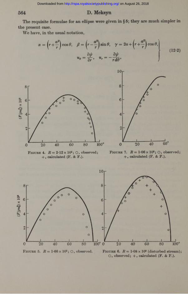
F —5 = 6-66 x 10-3. (11-7)pul

The final results, together with Fage & Falkner’s measurements and calculations, are given in figures 4 to 7 on p. 564.

As can be seen from the figures, our computed values are in good agreement with the observations, and in close agreement with Fage & Falkner’s computations for the ascending parts of the friction curves.

In the cases of R = 2-12 x 105, 1-66 x 105 and 1*08 x 105 (disturbed stream) the boundary layer becomes turbulent before separation; but, if the curves of the laminar surface friction are continued, they intersect the axis at about 92° from the stagnation point.

On the other hand, according to the simplified equation (11-1) separation is at about 94° from stagnation point.

As can be seen from figures 4 and 6 the agreement between the computed and observed values of surface friction is very satisfactory in both cases up to almost the separation point.

The case of the 6 in. cylinder {v0d/v = 0-943 x 105) considered by Green, Falkner & Thom (Fage & Falkner 1931, figure 6) was also solved; our results show close agreement with the above calculations in the ascending part of the friction curve.

12 . E v a l u a t io n o f dujdr a n d Aw0/Ar

To find the friction the velocity was measured at a very short distance from the surface, the relation between du0/dr and Aw0/Ar being found theoretically.

These quantities will now be derived for a particular case, and compared with Fage & Falkner’s results.

Consider the case

d = 5-89 in, u0 71-9ft./sec., u0d 2-12 xlO 5, 0 180°-30° 150°.

( 12- 1)v



x 10

s (

x 10

3The requisite formulae for an ellipse were given in §5; they are much simpler in

the present case.We have, in the usual notation,

564 D. Meksyn

Figure 4. R = 2-12 x 105; O, observed; Figure 7. = 1-06 x 10®; O, observed;+ , calculated (F. & F.). + , calculated (F. & F.).

Figure 5. R =1-66 x 106; O, observed.Figure 6. R = 1*08 x 108 (disturbed stream); O, observed; + , calculated (F. & F.).




accordingly dxjrdoc d\Jfd/3 dx{fdp . a . „U° = £ T r + T d = M = W Smd = U° i M (12-3)

since doc9/# a • a *■ -— = 0, 2 smd, at r ~ a, (12-4)

and dxjfjd/i is given by (3*18),

SimilarlyAH & f AH ( S s) ‘ w A r ’

(12-5)

and from (12-3) — = ” 2 sin 0 . u0 car(12-6)

In the present case a = 2-945 in., Ar = 0-0025 in., (12-7)

since the velocity was measured at 0-0025 in. from the surface. Accordingly, after a few simple computations,

A<r = 444 — = 0-377. a(12-8)

We have now to find/'(ct-) and/"(0); to that end it is necessary to solve the equation

/ " + / / ’ = - r o ( ^ ^ ) o( i - r > - (12-9)

In the present case /dlog h2\ cos 6^°\ doc / 0 sin2 \d

(12-10)

whence from table 4 (at the end of the paper), by interpolation,

/"(0) = 1-192, /'(0-377) = 0-3835. (12-11)

Since (3-18) u j 2 u 0yd p 2 \ v y ) }{ h

(12-12)

it is found by differentiating ue (12-3) with respect to r, and making and (12-5)

d_Ugdr u^ ) ' f W e

Act

Ar u0f(o-),

use of (12*4)

(12-13)

whence

From (12-6)

dug _ 444 x 12 x 1-192x71-9 dr rc=a 2-945 1-55 x 105.

A ue 0-3835x 71-9x 12 Ar = 0-0025 1-32 x 105,

(12-14)

(12-15)

the ratio being 1-17; the corresponding values as given by Fage & Falkner (1931, p. 194) are 1-46 x 105 and 1-26 x 105 respectively, whence the ratio is 1-16.

For the case 0 = 180° —20° = 160° the calculated ratio is 1-17.



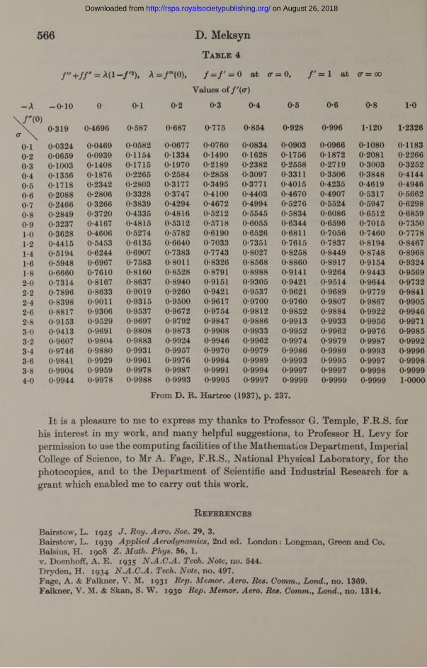
566 D. MeksynT a b l e 4

r+ir= A(i S ' 2), A=/'"(0), IIII 0 at <r II = 1 at a = 00

Values of f'(<x

- A -0 -1 0 0 0-1 0-2 0-3 0-4 0-5 0-6 0-8 1*0

\ / ' ( 0)

°-X \0-319 0-4696 0-587 0-687 0-775 0-854 0-928 0-996 1*120 1*2326

0-1 0-0324 0-0469 0-0582 0-0677 0-0760 0-0834 0-0903 0-0966 0-1080 0-11830-2 0-0659 0-0939 0-1154 0-1334 0-1490 0-1628 0-1756 0-1872 0-2081 0-22660-3 0-1003 0-1408 0-1715 0-1970 0-2189 0-2382 0-2558 0-2719 0-3003 0-32520-4 0-1356 0-1876 0-2265 0-2584 0-2858 0-3097 0-3311 0-3506 0-3848 0-41440-5 0-1718 0-2342 0-2803 0-3177 0-3495 0-3771 0-4015 0-4235 0-4619 0-49460-6 0-2088 0-2806 0-3328 0-3747 0-4100 0-4403 0-4670 0-4907 0-5317 0-56620-7 0-2466 0-3266 0-3839 0-4294 0-4672 0-4994 0-5276 0-5524 0-5947 0-62980-8 0-2849 0-3720 0-4335 0-4816 0-5212 0-5545 0-5834 0-6086 0-6512 0-68590-9 0-3237 0-4167 0-4815 0-5312 0-5718 0-6055 0-6344 0-6596 0-7015 0-73501 0 0-3628 0-4606 0-5274 0-5782 0-6190 0-6526 0-6811 0-7056 0-7460 0-77781*2 0-4415 0-5453 0-6135 0-6640 0-7033 0-7351 0-7615 0-7837 0-8194 0-84671*4 0-5194 0-6244 0-6907 0-7383 0-7743 0-8027 0-8258 0-8449 0-8748 0-89681-6 0-5948 0-6967 0-7583 0-8011 0-8326 0-8568 0-8860 0-8917 0-9154 0-93241-8 0-6660 0-7610 0-8160 0-8528 0-8791 0-8988 0-9141 0-9264 0-9443 0-95692-0 0-7314 0-8167 0-8637 0-8940 0-9151 0-9305 0-9421 0-9514 0-9644 0-97322-2 0-7896 0-8633 0-9019 0-9260 0-9421 0-9537 0-9621 0-9689 0-9779 0-98412-4 0-8398 0-9011 0-9315 0-9500 0-9617 0-9700 0-9760 0-9807 0-9867 0-99052-6 0-8817 0-9306 0-9537 0-9672 0-9754 0-9812 0-9852 0-9884 0-9922 0-99462-8 0-9153 0-9529 0-9697 0-9792 0-9847 0-9886 0-9913 0-9933 0-9956 0-99713 0 0-9413 0-9691 0-9808 0-9873 0-9908 0-9933 0-9952 0-9962 0-9976 0-99853-2 0-9607 0-9804 0-9883 0-9924 0-9946 0-9962 0-9974 0-9979 0-9987 0-99923-4 0-9746 0-9880 0-9931 0-9957 0-9970 0-9979 0-9986 0-9989 0-9993 0-99963-6 0-9841 0-9929 0-9961 0-9976 0-9984 0-9989 0-9993 0-9995 0-9997 0-99983-8 0-9904 0-9959 0-9978 0-9987 0-9991 0-9994 0-9997 0-9997 0-9998 0-99994-0 0-9944 0-9978 0-9988 0-9993 0-9995 0-9997 0-9999 0-9999 0-9999 1-0000

From D. R. Hartree (1937), p. 237.

It is a pleasure to me to express my thanks to Professor G. Temple, F.R.S. for his interest in my work, and many helpful suggestions, to Professor H. Levy for permission to use the computing facilities of the Mathematics Department, Imperial College of Science, to Mr A. Fage, F.R.S., National Physical Laboratory, for the photocopies, and to the Department of Scientific and Industrial Research for a grant which enabled me to carry out this work.

R e f e r e n c e s

Bairstow, L. 1925 J . Roy. Aero. Soc. 29, 3.Bairstow, L. 1939 Applied, A e r o d y n a m i c s ,2nd ed. London: Longman, Green and Co.Balsius, H. 1908 Z. Math. Phys. 56, 1.v. Doenhoff, A. E. 1935 N .A.C .A . Tech. Note, no. 544.Dryden, H. 1934 N .A.C .A . Tech. Note, no. 497.Fage, A. & Falkner, V. M. 1931 Rep. Mentor. Aero. Res. Comm., Lond., no. 1369. Falkner, V. M. & Skan, S. W. 1930 Rep. Memor. Aero. Res. Comm., Lond., no. 1314.



567

Goldstein, S. 1930 Proc. Camb. Phil. Soc. 26, 1.Goldstein, S. 1938 Modern Developments in Fluid Dynamics. Oxford: Clarendon Press. Green, J. J. 1930 Rep. Memor. Aero. Res. Co., Lond., no. 1313.Hartree, D. R. 1937 Proc. Camb. Phil. Soc. 33, 223.Hiemenz, K. 1911 Dinglers J . 326, 321.Howarth, L. 1934 Rep. Memor. Aero. Res. Comm., Lond., no. 1632.Howarth, L. 1938 Proc. Roy. Soc. A, 164, 547.v. Karman, Th. 1921 Z. angew. Math. Mech. 235.v. Karman, Th. & Millikan, C. B. 1934 N .A.C .A . Tech. Rep. no. 504.Millikan, C. B. 1936 J . Aero. Sci. 3, 91. v. Mises, R. 1927 Z. angew. Math. Mech. 425.Piercy, N. A. V., Preston, J. H. & Whitehead, L. G. 1938 Phil. Mag. 26, 791.Polhausen, K. 1921 Z. angew. Math. Mech. 252.Prandtl, L. 1904 Proc. I l l r d Int. Math. Congr. (Heidelberg), p. 484.Prandtl, L. & Betz, A. 1927 Vier Abhandlungen zur Hydrodynamik und Aerodynamik.

Gottingen: Kaiser Wilhelm Institut.Schubauer, G. B. 1935 N .A .C .A . Tech. Rep. no. 527.Thom, A. 1928 Rep. Memor. Aero. Res. Comm., Lond., no. 1176.Weyl, H. 1941 Proc. Nat. Acad. Sci., Wash., 27, 578.

The laminar boundary-layer equations. I

The laminar boundary-layer equations

II. Integration of non-linear ordinary differential equations

B y D . M e k s y n , D .S c .

(Communicated by G. Temple, F.R.S.—Received 3 June 1947)

1. T h e p r o b l e m

The aim of this paper is to find particular integrals of non-linear differential equations which satisfy certain boundary conditions and tend exponentially to zero at infinity.

The equations arise in connexion with the problem of integration of the equations of laminar flow in two dimensions.

The paper consists of two parts. In the first part the equation

/" '+ / / ' = A (1 - /'2)

is discussed, where A is generally a known parameter, and the primes denote deviations with respect to the independent variable, x.

This is the well-known Falkner & Skan’s (1930) equation. It was derived in connexion with the solution of the boundary-layer problem for a particular distribution of the velocity outside the boundary layer.

It appears, however, that this equation is of far more fundamental importance in the problem of laminar flow, although, of course, A has a different meaning in the general case than it has in Falkner & Skan’s treatment.



the laminar boundary-layer equations, i. motion of...

Documents