The Landsat Image Mosaic of Antarctica 1 2 3 4 5

(accepted for publication in emote Sensing of Environment) Robert Bindschadler, NASA Goddard Space Flight Center (Greenbelt, MD 20771,

Robert.A.Bindschadler@nasa.gov, 301-614-5707) 6

7

8

9

10

11

12

13

14

15 16

17

18

19

20

21

22

23

24

25

26

27

Patricia Vornberger, SAIC

Andrew Fleming, British Antarctic Survey

Adrian Fox, British Antarctic Survey

Jerry Mullins, USGS

Douglas Binnie, USGS EROS Data Center

Sara Jean Paulsen, USGS EROS Data Center

Brian Granneman, USGS EROS Data Center

David Gordetzky, ITT Visual Information Systems

Abstract The Landsat Image Mosaic of Antarctica (LIMA) is the first true-color, high-spatial-

resolution image of the seventh continent. It is constructed from nearly 1100 individually

selected Landsat-7 ETM+ scenes. Each image was orthorectified and adjusted for

geometric, sensor and illumination variations to a standardized, almost seamless surface

reflectance product. Mosaicing to avoid clouds produced a high quality, nearly cloud-

free benchmark data set of Antarctica for the International Polar Year from images

collected primarily during 1999-2003. Multiple color composites and enhancements

were generated to illustrate additional characteristics of the multispectral data including:

the true appearance of the surface; discrimination between snow and bare ice; reflectance

variations within bright snow; recovered reflectance values in regions of sensor

saturation; and subtle topographic variations associated with ice flow. LIMA is viewable

and individual scenes or user defined portions of the mosaic are downloadable at

http://lima.usgs.gov. Educational materials associated with LIMA are available at 28

http://lima.nasa.gov. 29

1

Introduction 30

31

32

33

34

35

36

37

38

39

40

41

42

43

44

45

46

Landsat imagery represents the oldest continuous satellite data record of the Earth’s

changing surface. Milestones in this record are represented by the production of mosaics

of all the continents, except Antarctica, for epochs of 1990 and 2000

(http://glcf.umiacs.umd.edu/portal/geocover/). The exclusion of Antarctica was dictated

more by financial constraints than interest; however the rapid changes of Antarctica that

are reported at increasing frequency and the advent of the International Polar Year

increase the value of completing the suite of continental Landsat mosaics with a

compilation of the southernmost continent.

The Long Term Acquisition Plan (Arvidson et al., 2001), used to manage the scheduling

of imagery from the Enhanced Thematic Mapper Plus (ETM+) sensor on-board the

Landsat-7 satellite, included the annual collection of thousands of Landsat images of

Antarctica beginning in 1999. These data form the basis of the mosaic described here. It

is referred to as the Landsat Image Mosaic of Antarctica (LIMA)

There were many steps required to produce the final products that are now publicly

viewable and available on the web site http://lima.usgs.gov/. These steps are described

here to give interested users a more complete understanding of the reasoning and the

methods applied in the selection, processing, enhancement and management of the nearly

1100 individual images that comprise LIMA, as well as a description of the variety of

mosaic products and metadata. The primary steps include: scene selection, Level-1

47

48

49

50

51

2

52

53

54

55

56

57

58

59

60

61

62

63

64

65

66

processing; conversion to surface reflectance; mosaicing (cloud removal and image

merging); enhancements; and web service. Each step is described in this document.

The care employed in the production of LIMA has resulted not only in the first-ever true-

color, high-resolution mosaic of the Antarctic ice sheet, but of a mosaic where each pixel

retains accurate values of surface reflectance. The producers of LIMA have resisted the

temptation to blend scene boundaries and artificially create color balance by either

uncontrolled or irreversible digital adjustments. As a result, LIMA is more than a pretty

picture that can only guide scientists to the original data, rather LIMA can be used

directly as a valid scientific data set. At the same time, it serves the public’s appetite for

a realistic view of the largest ice sheet and the coldest, highest and brightest continent on

Earth.

Scene Selection

Landsat-7 ETM+ scenes were the preferred source of all LIMA data for three principal

reasons: the geo-location of the data has been characterized to have a one-sigma accuracy

of + 54 meters (Lee and others, 2004); extensive imaging campaigns of Antarctica

undertaken soon after the April 1999 launch of Landsat-7 provided a large number of

available images during the first few years of sensor operations; and the existence of a

15-m panchromatic band provided the highest spatial resolution available with any

Landsat sensor.

67

68

69

70

71

72

73

74

Individual scenes to be used in LIMA were selected from the database of browse images

representing all Antarctic Landsat-7 scenes. The full collection of Antarctic browse

3

images are available through the USGS (http://edcsns17.cr.usgs.gov/EarthExplorer/) and

also were on hand at Goddard Space Flight Center, having been used for manual cloud

cover assessment. Each browse image is a composite of spectral bands 5, 4, and 3 (see

75

76

77

http://landsathandbook.gsfc.nasa.gov/handbook.html for a description of spectral

characterization of the ETM+). (Here, multiple-band composites will be identified in the

usual manner of three numbers whose order represents the bands assigned to the red,

green and blue channels, respectively). These browse images are in a compressed jpeg

format with an effective spatial resolution of 240 meters and provide a good indication of

clouds, if present. They do not allow the discrimination of smaller features or very thin

cloud.

78

79

80

81

82

83

84

85

86

87

88

89

90

91

92

93

94

95

96

97

A number of factors were weighed in the decisions of which scenes to use in LIMA.

Surface coverage (therefore, minimal cloud cover) obviously was very important, but

date and year of acquisition, especially of coastal scenes where large date differences

emphasized changes in the sea ice cover, was also considered. Selection decisions

attempted to minimize large variations in sun elevation of adjacent scenes. To minimize

the number of scenes, minimal overlap was sought; however, the geolocation details of

individual scenes were not available. Instead, the mean coordinates for every World

Reference System-2 scene was assigned to the browse image and a public-domain

software package (Geomatica FreeView V9.1) was used to compile a working version of

the emerging mosaic. In some cases, the most desirable Landsat-7 scene available

contained Scan Line Corrector-off data gaps

(http://landsat.usgs.gov/data_products/slc_off_data_products/index.php). In all, LIMA

4

98

99

100

101

102

103

104

105

106

107

108

109

110

contains 1073 Landsat-7 images (only 39 with SLC-off): 397 from the 1999-2000 austral

summer, 75 from the 2000-2001 austral summer, 220 from the 2001-2002 austral

summer, 342 from the 2002-2003 austral summer and 39 from later summers. Figure 1

illustrates the distribution of images used to generate LIMA, along with color

representing the range of sun elevations. Landsat coverage has a southern limit at 82.5oS.

To complete the continental coverage with a more pleasing visual product, data from the

MODIS Mosaic of Antarctica (Haran et al., 2005) were used in a manner described later

in this paper.

At one stage, a small number of ASTER images were considered as a viable means to

replace a cloudy portion of Landsat images, however, in the final analysis, the color

balancing became too difficult and the ASTER scenes were omitted from the final

mosaic.

5

111

112

113

114

115

116

117

118

119

120

121

122

123

124

Figure 1. Scenes selected for use in LIMA. Dot color indicates sun elevation value. In

36 cases there were multiple images from the same path/row location: 32 with two

images each and 4 with three images each. In these cases, the highest sun elevation

value is shown.

Level-1 Processing

All scenes selected for LIMA were processed from the Level-0 raw data to a Level-1T

orthorectified product using the National Landsat Archive Processing System (NLAPS)

at EROS (details at http://edc.usgs.gov/guides/images/landsat_tm/nlaps.html). Three

digital elevation models (DEMs) were investigated to supply the elevation data necessary

for orthorectification: the Radarsat Antarctic Mapping Project (RAMP version-2) DEM,

(http://nsidc.org/data/nsidc-0082.html); the ICESat DEM (http://nsidc.org/data/nsidc-

0304.html) and a combined radar altimeter-ICESat DEM (provided by J. Bamber).

6

125

126

127

128

129

130

131

132

133

134

135

136

137

138

139

140

141

142

143

144

145

The three DEMs were intercompared at a 5-km resolution (the supplied post spacing of

both the ICESat and radar altimeter-ICESat DEMs). Differences were examined to help

discern how they might affect the orthorectification process in different parts of

Antarctica. The deciding factors were coverage and accuracy in mountainous regions.

The ICESat DEM was not complete to all edges of the continent, and the radar altimeter-

ICESat DEM was not able to include the extreme topographic variations of the

mountainous regions. Because Landsat’s field of view is nadir and near-nadir, ortho-

rectification corrections are largest in areas of high relief and at the scene edges. For

these reasons, the RAMP version-2 DEM, which also is available on a much finer 200-m

spacing, was selected for orthorectification in the NLAPS processing stream.

Conversion to Surface Reflectance

Many steps were required to convert the radiance measured at the ETM+ sensor to an

accurate value of surface reflectance. These are discussed below in the order they were

applied to the NLAPS-processed data.

Saturation Adjustment

The high reflectance of snow at optical wavelengths can saturate the ETM+ sensor.

Saturation radiance thresholds vary by band, by gain setting (High or Low) and by

illumination geometry (sun elevation and surface slope). Table 1 indicates the saturation

radiance, Lmax, for ETM+ bands (both High and Low gain setting).

7

Table 1. ETM+ Spectral Radiance Range (W/(m2 * ster * μm)), from Table 11.2 in 146

http://landsathandbook.gsfc.nasa.gov/handbook/handbook_htmls/chapter11/chapter11.ht147

ml 148

149

ETM+ Spectral Radiance Range

watts/(meter squared * ster * μm)

Before July 1, 2000 After July 1, 2000

Low Gain High Gain Low Gain High Gain Band

Number LMIN LMAX LMIN LMAX LMIN LMAX LMIN LMAX

1 -6.2 297.5 -6.2 194.3 -6.2 293.7 -6.2 191.6

2 -6.0 303.4 -6.0 202.4 -6.4 300.9 -6.4 196.5

3 -4.5 235.5 -4.5 158.6 -5.0 234.4 -5.0 152.9

4 -4.5 235.0 -4.5 157.5 -5.1 241.1 -5.1 157.4

5 -1.0 47.70 -1.0 31.76 -1.0 47.57 -1.0 31.06

6 0.0 17.04 3.2 12.65 0.0 17.04 3.2 12.65

7 -0.35 16.60 -0.35 10.932 -0.35 16.54 -0.35 10.80

8 -5.0 244.00 -5.0 158.40 -4.7 243.1 -4.7 158.3

150

8

151

152

153

154

155

156

157

158

159

160

161

162

163

164

165

166

167

168

169

170

171

172

173

The spectral reflectance of snow varies with the specific type of snow (primarily snow

grain size and wetness). In general, snow is most reflective in Band 1, decreasing

through Bands 2 and 3, decreasing to even lower values in Band 4 and decreasing to very

low values in Bands 5 and 7 (see Dozier and Painter, 2004, for a review of multispectral

remote sensing of snow). As snow ages, the snow grain size increases, and reflectance

decreases at all optical wavelengths.

Failure to adjust for saturation will cause saturated image pixels to be converted to an

incorrect spectral reflectance that is lower than the actual reflectance, and produce false

colors in multi-band composite images. Saturation adjustment is completed before any

other adjustment because it is easiest to identify saturation at this early stage of image

processing by the test condition that a pixel value is saturated (Digital Number (DN) =

255, the maximum value for the 8-bit data range of ETM+). DNs correspond to a band-

specific scaled radiance value, but the conversion to radiance is made after the saturation

adjustment discussed here.

Saturation values (DN=255) of a given pixel are adjusted to DN values greater than 255

by applying a predetermined spectral ratio to an unsaturated band value at the same pixel.

The appropriate spectral ratio was determined by examining 27 Landsat scenes across

Antarctica that were selected to provide a variety of surfaces, a variety of sun elevation

values and all three gain combinations of spectral bands used for ETM+ acquisitions of

Antarctica (see Figure 2 and Table 2).

9

174

175

176

177

178

179

180

181

182

183

184

185

186

Figure 2. Location of 27 Landsat ETM+ scenes used to determine empirical relationships

for saturation adjustment and non-diffusive reflectance of LIMA images. Numbers in

scene outline boxes refer to sun elevation at center of each scene.

The distribution of DN for snow pixels within each image was checked to be normally

distributed and the DN of the histogram peak for each band in each scene was identified.

The DN value of the histogram peak depended strongly on sun elevation, with lower DN

values for lower sun elevations (Figure 3). Band 1 always had the highest snow-

histogram maximum DN value, Band 3 was somewhat lower, then Band 2, followed by

Band 8. The relative position of Band 4 depended on its gain setting—the gains of Bands

1, 2 and 3 were always either all High or all Low, depending on sun elevation, while

Band 4 was switched independent of any other band. Band 8 always remained at Low

10

187

188

gain. Bands 5 and 7 were not considered. These interband relationships are consistent

with snow spectra of aging snow collected in the field (Dozier and Painter, 2004).

189

190

191

192

193

194

195

196

197

198

199

200

Figure 3. DN of the snow histogram maximum plotted versus sun elevation for each

band of the 27 ETM+ scenes indicated in Figure 1. Gain settings for Bands 1-4 and 8,

indicated by H (high) and L(low) along the bottom of the plot, were tied to sun elevation.

Band-to-band spectral ratios were calculated from the data plotted in Figure 3. They are

very consistent for the same gain combination and indicate no dependence on sun

elevation (Figure 4). These ratios are also given in Table 2. Their consistency forms a

sound basis for our saturation adjustment methodology.

11

201

202

203

204

205

206

Figure 4. Band-to-band ratios versus sun elevation derived from Figure 3 values.

Table 2. Spectral band ratios of DN for snow regions of the 27 sample scenes indicated

in Figure 2. Gain settings are given as High (H) or Low (L) in order of bands 1-4 and 8.

Band Ratio HHHHL LLLHL LLLLL

Band1/Band2 1.2130 1.1794 1.1794

Band3/Band2 1.1058 1.0858 1.0858

Band1/Band8 1.9460 1.2831 1.2831

Band2/Band8 1.6048 1.0944 1.0944

Band3/Band8 1.7743 1.1814 1.1814

Band4/Band8 1.2315 1.1806 0.7728

207

12

208

209

210

211

212

213

214

215

216

217

218

219

220

221

222

223

224

225

226

227

In applying this saturation adjustment to the LIMA scenes, every pixel in every scene

was examined for saturation in the following band order: 1, 3, 2, 4. If saturation was

identified (DN=255), then the pixel’s value in Band 2 is used along with the appropriate

spectral band ratio (depending on the relative gain settings, see Table 2) to adjust the

saturated DN value to a higher value based on the DN value of the unsaturated band. If

Band 2 is also saturated, then Band 8 is used, with the appropriate spectral ratio (see

Table 2).

Sensor Radiance to Surface Reflectance Conversion

The ETM+ sensor was frequently calibrated to maintain an accurate conversion of the DN

value to the at-sensor radiance (see Chapter 9 of the Landsat-7 Science Data Users

Handbook at http://landsathandbook.gsfc.nasa.gov/handbook/handbook_toc.html). These

calibration coefficients are included in the header files of every NLAPS-processed

Landsat scene. The conversion from DN to at-satellite radiance is accomplished by

applying the following equation:

L(λ) = {[Lmax(λ) – Lmin(λ)]/255} * DN + Lmin(λ) (1)

Where L(λ) is the spectral radiance at the sensor’s aperture, and Lmin(λ) and Lmax(λ) are

the spectral radiances that correspond to DN=0 and DN=255, respectively (see Table 1).

Radiances are given in W/m2*ster*μm.

From these calibration values, the conversion of at-sensor radiance to planetary

reflectance follows from:

13

sSEdLθλ

λπρcos)()( 2

= (2) 228

229

230

231

232

233

234

235

236

237

238

239

240

241

242

243

244

245

246

247

Where ρ is planetary reflectance, d is the Earth-Sun distance (in AU), Es(λ) is the mean

solar exoatmospheric irradiance, and ϑs is the solar zenith angle (in degrees) (see Chapter

11 of the Landsat-7 Science Data Users Handbook).

Converting planetary reflectance to surface reflectance usually involves the use of an

atmospheric scattering model. Such models require input values of atmospheric water

vapor and aerosols. The atmosphere over most of the Antarctic continent is very cold,

minimizing the amount of water vapor, and very clean, minimizing the concentration of

aerosols. The assumption made here is that these atmospheric corrections are negligible

and the planetary reflectance is a good approximation of the surface reflectance.

The cosine dependence of the surface brightness results from the fact that the illuminated

surface area per solid angle of incoming solar radiation varies with the cosine of the sun

elevation angle. This situation strictly only applies for a horizontal surface. For sloping

surfaces, the slope component in the direction of the solar illumination must be added to

the sun elevation angle. It is this additional factor that allows the surface topography of

the ice sheet to be visually discerned by brightness variations in Landsat images of the ice

sheet. Calculated reflectance values in excess of unity are not uncommon in sloping

snow covered terrain when the surface slope is not included in Equation 2.

14

Local Sun Elevation Adjustment 248

249

250

251

252

253

254

255

256

257

258

259

260

261

262

263

264

265

266

267

268

269

270

At high latitudes, the local sun elevation varies significantly (i.e., a few degrees) across a

Landsat scene. This requires the solar elevation in Equation 2 to be the local sun

elevation angle at each pixel and not the scene-center value. The local sun elevation

angles are calculated by using a solar ephemeris to calculate the solar elevation at each of

the four scene corners for the time and date of the scene center. The solar elevation at

each pixel is then calculated using a bi-linear interpolation of the four scene-corner sun

elevations.

Correction for non-Lambertian Reflectance

The DN-to-surface reflectance conversion represented by Equation 2 assumes the

reflectance character of the surface is Lambertian and that the Landsat sensor views the

surface from directly overhead. While the second assumption is generally valid, even at

the image edges, the first is not. At progressively lower sun elevations, snow deviates

from the properties of a Lambertian, perfectly diffusive reflector due to increasing

forward scattering (Warren et al., 1998, Masonis and Warren, 2001).

Field studies of this effect provide limited quantitative estimates of this non-Lambertian

effect. We also draw upon an empirical form of this relationship based on the same 27

Landsat scenes referenced above (Figure 2). Figure 5 shows how the surface reflectance,

calculated from Equation 2, varies with sun elevation. In this figure, the Band 1

reflectance decreases as sun elevation increases beyond 27 degrees and Band 2 and 3

reflectances decrease as sun elevation increases beyond 31 degrees due to saturation.

These decreases are not a real effect, rather, they are the result that a saturated sensor

15

271

272

reading of 255 underestimates the actual at-sensor radiance and this underestimate of

radiance is converted, through Equation 2, to an underestimate of reflectance.

273

274

275

276

277

278

279

280

281

282

Figure 5. Surface reflectance versus sun elevation for the 27 Landsat scenes

indicated in Figure 2. Surface reflectances are calculated from Equation 2 without

any saturation adjustment applied.

Saturation adjustment, as described above, corrects the artificial surface reflectance

decrease at higher sun elevations (Figure 6). What remains is the non-Lambertian effect

of decreasing surface reflectance as sun elevation decreases. This affects nearly all sun

elevations in the LIMA data set, becoming marginal for sun elevations above 30 degrees.

16

283

284

285

286

287

288

289

290

291

292

293

294

295

296

Figure 6. Surface reflectance versus sun elevation (see Figure 5) after saturation

adjustment.

Our adjustment for the non-Lambertian reflectance effect takes the form of an adjustment

ratio for each spectral band. The purpose of this adjustment is to increase the calculated

reflectances at lower sun elevations to what the reflectance would have been if the

surface were a Lambertian reflector or if they had been illuminated with the same solar

elevation. These ratios were determined initially by fitting quadratic curves to the non-

saturated data pairs of surface reflectance versus sun elevation, i.e. by fitting the data in

Figure 6 with quadratic curves, and dividing those fitted values by a “standard”

reflectance value for each band. The initial ratios contained slight biases that were

subsequently removed by fitting a line to the adjusted reflectances and modifying the

ratios so that the mean of the adjusted reflectances for each band matched the standard

17

297

298

299

300

301

302

303

304

305

306

reflectances. We found that our derived reflectance values agreed with field data for a

sun elevation of 31 degrees (Masonis and Warren, 2001), so we defined a set of

“standard” reflectances, given in Table 3. The field data are limited to 600nm

wavelength—in the absence of other field data we assume here that a similar correlation

applies at all wavelengths. The resulting ratio values are shown in Figure 7 along with a

similarly calculated set of ratios for the field data. Surface reflectances calculated for

saturated pixels are included in Figure 6, but excluded from the quadratic fits and the

non-Lambertian adjustment ratios.

Table 3. “Standard” spectral reflectance for snow

Band 1 0.9362

Band 2 0.8694

Band 3 0.8697

Band 4 0.8599

Band 8 0.8556

307

18

308

309

310

311

312

313

314

315

316

317

318

319

320

321

Figure 7. Non-Lambertian adjustment ratio versus sun elevation derived from 27

Landsat scenes shown in Figure 1 and for field data (from Masonis and Warren,

2001).

Reflectance Normalization

Our final adjustment to surface reflectance is not physically based, but motivated by the

desire to produce a visually consistent mosaic by eliminating visually distracting edges

between adjacent scenes. LIMA unavoidably includes scenes with slight differences in

actual surface conditions. To minimize reflectance “offsets”, we perform a final

“normalization” adjustment to match the mean snow reflectance of each scene to the

“standard” spectral reflectances described above (cf. Table 3).

To implement this final adjustment, the reflectance histogram of each scene is quantified

for each band using a reflectance binning interval of 0.004. Once quantified, the

19

322

323

324

325

326

327

328

329

330

331

histogram bin above 0.5 reflectance that has the greatest number of occurrences (i.e., the

mode) is determined, and the reflectance value of that bin is compared with the

corresponding “standard” spectral reflectance. A “reflectance normalization” ratio (equal

to the “standard” reflectance divided by the actual reflectance) is then applied to the

entire scene to force the mode of the distribution of reflectance values to match the

“standard” spectral reflectance. A ratio approach is used to minimize the changes for

lower reflectance regions, e.g. rock.

After accounting for all of the above adjustments, the actual equation that is applied is of

the same form as Equation 2, but modified to the following:

SRNLsS

ffE

dLθλ

λπρcos)()( 2

= (3) 332

333

334

335

336

337

338

339

340

341

342

343

where fNL is the adjustment ratio for non-Lambertian reflectance, and fSR is the histogram-

based “reflectance normalization” adjustment ratio to the “standard” snow reflectances.

These spectral reflectance shifts are recorded in an ancillary data file to ensure that the

adjustments are preserved and are available to LIMA users in a metadata file.

Reserving the non-physical adjustment to the last of the series of adjustments described

in this section provides a measure of the success of the physically-based adjustments in

creating a high-quality data set of actual reflectance values. In practice, most LIMA

scenes did not require any significant normalization adjustment. Of the 4292 values of

fSR (4 bands for each of 1073 scenes), only 9% required a “reflectance normalization”

adjustment ratio greater than 1.05 or less than 0.95, mostly in Band 4.

20

Mosaicing 344

345

346

347

348

349

350

351

352

353

354

355

356

357

358

359

360

361

362

363

364

365

366

Once the individual scenes were adjusted, they were mosaiced together using customized

software developed by ITT VIS to be used within the ENVI image processing

environment. The mosaicing procedure began by determining a stacking order of scenes

(the single value of any pixel comes from the uppermost scene with a value for that pixel)

and then omitting unwanted portions of scenes, such as clouds, to allow preferred

portions of scenes lower in the stack to show through. In practice, many clouds present

in the selected scenes were effectively removed by ensuring that another scene, with

corresponding cloud-free pixels was placed higher in the image stack.

Although every attempt was made to normalize the reflectances of all the scenes, the

adjustments detailed above were only performed to entire scenes. There were a few

instances where there were reflectance variations within a scene that caused a visual mis-

match between it and all its neighboring scenes. In this case, judicious trimming of scene

boundaries was employed to minimize these visually disruptive scene-to-scene jumps in

reflectance. Any residual mismatch in adjacent scene color balance was removed by

applying band-specific adjustments based on local histogram statistics. These

adjustments are recorded in the LIMA metadata and were required for only 62 of the

1073 scenes.

The most difficult area to produce a visually smooth mosaic was around the ice sheet

margin where temporal variations of the sea ice pack and changes in the extent of ice

shelves produced occasional discontinuities in adjacent scenes. Inevitably some

21

367

368

369

370

371

372

373

374

375

376

377

378

379

380

381

382

383

384

385

386

387

388

discontinuities remained, but these were minimized through suitable trimming and

stacking of adjacent scenes. Further there are a small number of areas where it was not

possible to identify suitable cloud free imagery and patches of cloud are still present. As

more suitable imagery of these regions becomes available these portions will be updated.

The data volume of so many scenes required that the mosaic be prepared in a series of 25

smaller blocks, each composed of 24 to 76 individual scenes. This “building block”

structure was incorporated into the mosaicing software allowing blocks, once completed,

to be combined through output instruction files into a larger mosaic. In fact, the full

continental mosaic never existed as a single file, rather only as a “virtual mosaic”—a

series of separate image files (each a combination of a few blocks) linked by a control file

that could guide subsequent operations on the mosaic exactly as if the mosaic actually did

exist in a single file. This approach avoided the need for extremely large files and the

associated storage and file input/output problems that can accompany very large files.

From this mosaicing operation and the virtual mosaics that were created (one for every

spectral band), a series of GeoTIFF tiles were created that covered the entire continent.

170 GeoTIFF tiles were produced, each within the upper file size limit of 2.14 gigabytes

for a “standard” GeoTIFF file. The tile pattern was created to ensure that the production

of the various multiband composites and contrast-stretched enhancements (described in

the next section) would also not exceed the GeoTIFF size limitation using the same tile

arrangement.

22

Data Precision 389

390

391

392

393

394

395

396

397

398

399

400

401

402

403

404

405

406

407

408

409

410

Any description of a new data set requires a careful explanation of data precision. This

topic perhaps is best presented at this juncture between the end of the data processing

procedures and the beginning of the generation of display products. Much earlier, it was

mentioned that the NLAPS processing of individual scenes produced multiband data with

8-bit precision. An 8-bit representation imposes an upper bound to the accuracy due to

the number of quantization levels. This quantization constraint is consistent with the

noise levels of the multispectral bands and of the panchromatic band of the ETM+ sensor,

approximately 1 DN and 2 DN, respectively (Scaramuzza et al., 2004).

All of the post-NLAPS processing steps described above carried a 16-bit level of

precision to the various data adjustments. This was important to allow these refinements

to have their full effect and not be lost in truncations or roundings of the very last bit of

the 8-bit data values. With the extra range afforded by 16-bit data, the spectral

reflectances are calculated to the nearest 0.0001 (i.e., a value of 10,000 represents a

reflectance of unity). To preserve the highest level of LIMA image quality, the 16-bit

mosaics of each spectral band are available.

Most computer displays require 8-bit gray-scale signals, or 24-bit color signals (three

bands for the red, green and blue color guns, each in 8-bit). For this reason, the various

display products described below are all generated as 8-bit single band, or 24-bit color

composites.

23

Enhancements 411

412

413

414

415

416

417

418

419

420

421

422

423

424

425

426

427

428

429

430

Digital imagery enables enhancement of the visual representation of the digital data

through the use of different assignments of the original data values to those displayed on

a computer monitor. These methods are very appropriate to LIMA where so many of the

snow surface features occur in a very narrow range of reflectances and dark rock lies

adjacent to bright snow. This section describes the various techniques employed to allow

the user to see more of the digital content of LIMA. Ultimately, the availability of the

LIMA data in 16-bit digital form allows users unlimited possibilities for additional

enhancements.

Figure 8 is a reflectance histogram of a typical scene fully processed for LIMA. It

includes a very large but narrow peak for snow pixels that dominate the Antarctic surface

(note the scale change on the vertical axis), a much smaller peak at low reflectance

(corresponding to dark rock), includes pixels with reflectances between these two peaks,

as well as some pixels with reflectances above unity (10,000 in 16-bit values). Few

reflectances exceed 1.60 (16,000 in 16-bit values) and no reflectance value is less than

0.0001 (1 in 16-bit value) (the value zero is reserved to represent “no data”). The

reflectance at the histogram peak is 0.8728. These histogram values become important in

the enhancements to follow.

24

431

432

433

434

435

436

437

438

439

440

441

442

443

Figure 8. Representative histogram of 16-bit reflectance values for a LIMA scene.

There is a scale change on the vertical axis to capture both the full extent of the

major histogram peak as well as the detail at other reflectance values.

Pan-Sharpening

The LIMA enhancements begin with “pan-sharpening” to increase the spatial resolution

of the spectral bands. This involves applying the finer spatial variations of the 15-meter

spatial resolution panchromatic band (Band 8) to the 30-meter resolution narrower

spectral bands (Bands 1-4). A key characteristic of the spectral and panchromatic bands

is that they are coregistered. The upper left corners of the upper left pixels of each band

are co-located. From that common point, all pixels of all the 30-meter spectral bands are

also co-located. The panchromatic band has its 15-meter pixels nested within the 30-

25

444

445

446

447

448

449

450

451

452

453

454

455

456

457

458

459

460

461

462

463

464

465

466

meter pixels such that every 2 x 2 square of panchromatic pixels matches the location of a

30-meter pixel.

This convenient alignment is used to increase the resolution of the spectral bands with a

simple algorithm. Each 30-meter spectral band pixel is subdivided into four 15- meter

pixels. For a specific pixel, let S be the initial pixel value and let s1, s2, s3 and s4 be the

values to be assigned to the 15-meter subdivided pixels. The four panchromatic pixel

values (p1, p2, p3, p4) are averaged together to a mean value of P and the spectral values

are then calculated as:

s1 = S * p1/P

s2 = S * p2/P

s3 = S * p3/P

s4 = S * p4/P

This formulation has the additional property that the original 30-meter spectral values can

be recovered by averaging the pan-sharpened 15-meter pixels.

Base Composites

Color composites are produced by converting the single-band, pan-sharpened 16-bit

values at each pixel to 8-bit single band values and combining three bands into a 24-bit

color product. An 8-bit number cannot be larger than 255 (starting at 0). To compress

the 16-bit range of reflectances into this narrower range, each 16-bit reflectance value (in

hundredths of percent) between 0 and 10,000 is divided by 40. Thus, 100% reflectance is

converted to a value of 250. To convert any 8-bit value to the corresponding reflectance

26

467

468

469

470

471

472

value (in percent), it must be divided by 2.5. Reflectances in 16-bit data above 10,000

(and below the maximum value of 16,000) are converted to 8-bit values between 250 and

255.

The specific equations used are:

r = R/40 0<R<10,000 473

474 r = R/1200 + 241.67; 10,000<R<16,000

r = 255; 16,000<R 475

476

477

478

479

480

481

482

483

484

485

486

487

where R is the 16-bit value and r is rounded to the nearest 8-bit value excluding r=0. The

difference between the divisor of 40 for the reflectance range 0-100% and the divisor of

1200 for reflectances above 100% means that very bright reflectances (such as can occur

on the sun-lit sides of steep snow-covered mountains) are highly compressed into a very

narrow range of values in the 8-bit representation of LIMA. An example of this effect is

illustrated later and a later enhancement is designed to relax this data compression of very

bright values at the expense of compressing darker data pixels.

Figure 9 illustrates this 16-bit to 8-bit conversion by the thin black line. It matches any

16-bit number on the horizontal axis with the converted 8-bit number on the vertical axis.

27

488

489

490

491

492

493

494

495

496

497

498

499

500

501

502

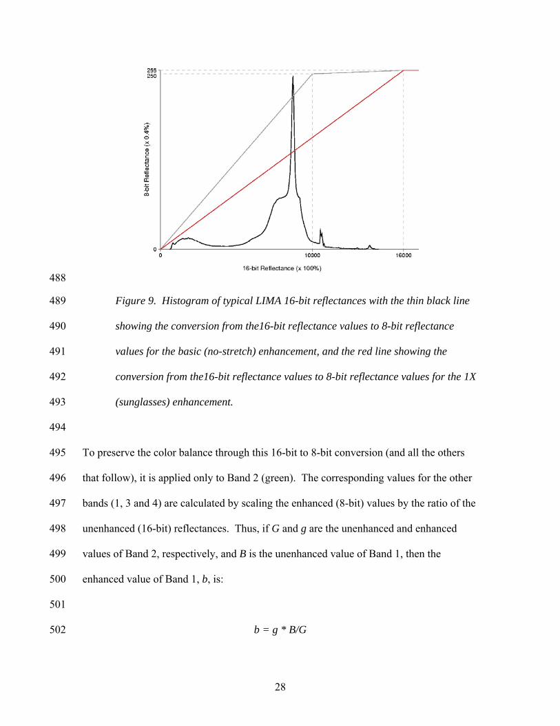
Figure 9. Histogram of typical LIMA 16-bit reflectances with the thin black line

showing the conversion from the16-bit reflectance values to 8-bit reflectance

values for the basic (no-stretch) enhancement, and the red line showing the

conversion from the16-bit reflectance values to 8-bit reflectance values for the 1X

(sunglasses) enhancement.

To preserve the color balance through this 16-bit to 8-bit conversion (and all the others

that follow), it is applied only to Band 2 (green). The corresponding values for the other

bands (1, 3 and 4) are calculated by scaling the enhanced (8-bit) values by the ratio of the

unenhanced (16-bit) reflectances. Thus, if G and g are the unenhanced and enhanced

values of Band 2, respectively, and B is the unenhanced value of Band 1, then the

enhanced value of Band 1, b, is:

b = g * B/G

28

503

504

505

506

507

508

509

510

511

512

513

514

Similar equations hold for Bands 3 and 4.

Two “base”, i.e., unenhanced, products are produced from this 16-bit to 8-bit conversion

of spectral Bands 1 through 4. One is a combination of Bands 3, 2, and 1 into the red,

green and blue channels. Because of the spectral locations of these bands, this produces a

true-color representation of LIMA data. The second base composite is a combination of

Bands 4, 3, and 2 into the red, green and blue channels. This “false-color” combination

holds some advantage over the true-color composite for discriminating between bare ice

(appearing more blue) and snow (that still appears white). Figure 10 illustrates a sample

of each composite.

515

516

517

518

519

Figure 10. Comparison of the 321 (left) and the 432 (right) color composites for

a region of North Victoria Land in East Antarctica. Each subimage is 7 km

across.

29

Enhancements 520

521

522

523

524

525

526

527

528

529

530

531

532

533

534

535

536

537

538

539

Subtle variations of the LIMA data set are not apparent visually in the base composites

because the human eye is not capable of resolving 256 different shades of any color.

Digital enhancements can be constructed to highlight selected portions of the reflectance

range so they can be seen more easily. To make these subtle details viewable, a set of

digital enhancements have been performed on the 16-bit bands prior to combining them

into additional true-color (321) and false-color (432) composites.

The first enhancement is designed to accentuate very bright reflectances (over 100%) that

were strongly compressed in the base composites. To accomplish this, the bilinear

enhancement of the base composites described above is modified to a single divisor of

62.745(=16,000/255). This enhancement has two major results. One is that the

reflectances above 100% are now represented by a larger portion of the 0-255 range of 8-

bit values, allowing the spatial variations to be seen more easily. The other result is that

the reflectances in the 0 to 100% range will not only be distributed over a smaller portion

of the 0-255 8-bit range than before, thus sacrificing some visual detail, but they will also

be represented by lower values, making these pixels appear darker than in the base

composites. The specific equations used are:

r = R/62.745 0<R<16,000

r = 255; 16,000<R 540

541

542

where R is the 16-bit value and r is rounded to the nearest 8-bit value excluding r=0.

30

543

544

545

546

547

548

549

The red line in Figure 9 illustrates this enhancement and helps illustrate why the snow

surfaces appear darker with the enhancement than in the base composites. An illustration

of the 1X enhancement is given in Figure 11. This enhancement acts much like wearing

a pair of sunglasses and so is termed the “sunglasses” enhancement. Both true-color

(321) and false-color (432) composites are formed from these enhanced bands.

550

551

552

553

554

555

556

557

558

559

Figure 11. LIMA sub-image of Mt. Takahe in West Antarctica with the 321 true-

color composite (left) and with the 1X “sunglasses” enhancement (right). Details

of the sun-facing slope appear “overexposed” in the left sub-image and more

visible in the 1X enhancement.

The remaining enhancements are all aimed at increasing the visual appearance of detail in

the flatter ice sheet surface which, in terms of relative area, dominates Antarctica. These

surfaces fall into the range of reflectances in the large histogram peak (see Figure 8)

31

560

561

562

563

564

565

566

567

568

569

570

571

572

573

574

whose central peak of 0.8728 reflectance converted to an 8-bit value of 139 in the

previous (1X) enhancement. This value is retained in these remaining enhancements

while the strength of the stretch (i.e., the slope of the line in the histogram figures) is

increased by factors of 3X, 10X and 30X. To use more of the 8-bit range to display these

details requires that some other portions of the full range of 16-bit reflectances be

compressed to increasingly narrower ranges of 8-bit values. We define a tri-linear

enhancement where the middle linear segment is centered on this 0.8728 reflectance (at

an 8-bit value of 139) and pivoted to various slope values. This central linear segment is

limited to the 8-bit range from 25 to 230. On either side of this central segment, another

linear segment converts the 16-bit values to 8-bit values of 1 to 25 for low reflectances,

and 230 to 255 for high reflectances.

In the 3X case, called the “low-contrast” enhancement, the specific equations applied are:

r = R/253.76; 0<R<6344

r = R/20.915 – 278.3075; 6344<R<10,631 575

576 r = R/214.76 + 180.498; 10,631<R<16,000

r = 255; 16,000<R 577

578

579

580

581

where R is the 16-bit value and r is the 8-bit value excluding r=0. Figure 12 illustrates

the nature of this enhancement superimposed on the representative histogram.

32

582

583

584

585

586

587

588

589

590

591

592

Figure 12. Histogram of typical LIMA 16-bit reflectances showing the conversion

from the16-bit reflectance values to 8-bit reflectance values for the 3X “low-

contrast”, 10X “medium-contrast”, and 30X “high-contrast” enhancements.

The “medium-contrast” enhancement provides an even stronger (10X) stretching of the

dominant ice-sheet surface reflectances to reveal even finer details of the snow surface.

The specific equations applied are:

r = R/320.52; 0<R<8013

r = R/6.2745 -1252.03; 8013<R<9299 593

594 r = R/268.04 + 195.307; 9299<R<16,000

r = 255; 16,000<R 595

596

33

where R is the 16-bit value and r is the 8-bit value excluding r=0. Because the

differences between the true-color and false-color composites are so slight, only a true-

color composite is produced.

597

598

599

600

601

602

603

604

605

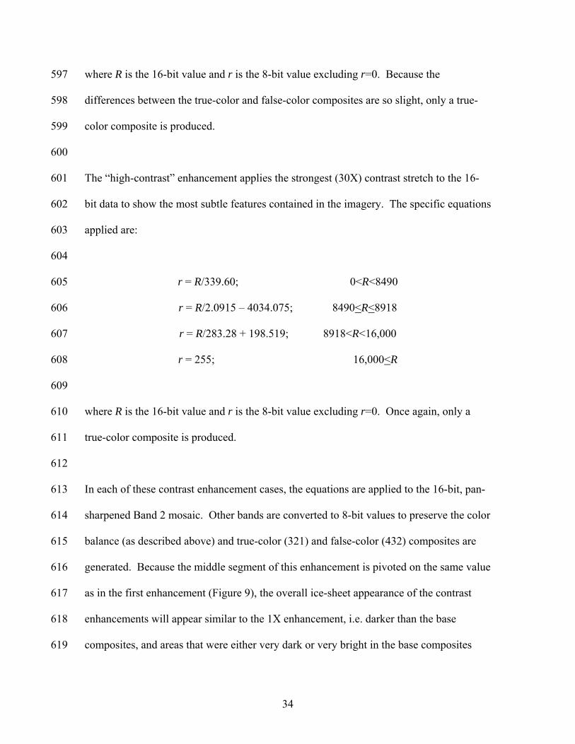
The “high-contrast” enhancement applies the strongest (30X) contrast stretch to the 16-

bit data to show the most subtle features contained in the imagery. The specific equations

applied are:

r = R/339.60; 0<R<8490

r = R/2.0915 – 4034.075; 8490<R<8918 606

607 r = R/283.28 + 198.519; 8918<R<16,000

r = 255; 16,000<R 608

609

610

611

612

613

614

615

616

617

618

619

where R is the 16-bit value and r is the 8-bit value excluding r=0. Once again, only a

true-color composite is produced.

In each of these contrast enhancement cases, the equations are applied to the 16-bit, pan-

sharpened Band 2 mosaic. Other bands are converted to 8-bit values to preserve the color

balance (as described above) and true-color (321) and false-color (432) composites are

generated. Because the middle segment of this enhancement is pivoted on the same value

as in the first enhancement (Figure 9), the overall ice-sheet appearance of the contrast

enhancements will appear similar to the 1X enhancement, i.e. darker than the base

composites, and areas that were either very dark or very bright in the base composites

34

620

621

622

will appear even darker and even brighter, respectively, in each contrast enhancement.

An example of the successively stronger contrast enhancements is shown in Figure 13.

623

624

625

626

627

628

629

630

631

632

633

634

635

Figure 13. Sample of the contrast enhancements progressing (left to right) from

no enhancement to 3X, 10X and 30X, for a portion of the megadune area of East

Antarctica. Each image is 12 km on a side.

Because LIMA is also available as 16-bit data product, users can apply a nearly limitless

variety of enhancements and image processing procedures tailored to the user’s interests

and objectives. An example of this is shown in Figure 14 where a customized

enhancement is applied to draw out details of ice flow features in a region where two

glaciers exit the Transantarctic Mountains and join as they enter the Ross Ice Shelf.

35

636

637

638

639

640

641

642

643

644

645

646

647

648

649

650

651

652

653

654

Figure 14. Sample of the customized enhancement of a region of two merging

glaciers showing the ability of the 16-bit LIMA data to reveal significant surface

detail. Left sub-image is the region in the 1X enhancement, middle sub-image is

after a strong enhancement, and the right sub-image is the same region cropped

from the MODIS Mosaic of Antarctica (MOA). Each image is 110 km on a side.

Complementary Mosaics

Although LIMA represents a significant addition to the ability to “see” Antarctica, we

view it as complementary to other existing mosaics. We have already mentioned the

MODIS Mosaic of Antarctica (Haran et al., 2005) and used it in the comparison in Figure

14. MODIS data have lower spatial resolution, but a wider field of view and more

radiometric resolution. This often enables clearer views of extensive surface features

where LIMA scene edges might begin to interrupt the larger view. On the other hand,

LIMA’s spatial detail can be instructive in probing the smaller feature limits of MOA.

Both LIMA and MOA were preceded by the continental scale mosaic of Antarctica

created from synthetic aperture radar data collected by Radarsat (Jezek et al., 2001).

36

655

656

657

658

659

660

661

662

Radar “speckle” reduces the effective spatial resolution of the Radarsat mosaic to close to

100 meters, but the dominant appearance of this mosaic is an emphasis on sharp edges,

such as surface crevasses or rugged topography. This emphasis can be exceptionally

useful in a variety of glaciological and geological studies and, again, the combination

with LIMA’s visual representation of the surface can introduce a high degree of synergy

in linked examinations of these data sets. Figure 15 illustrates the MOA and Radarsat

mosaics’ view of Mount Takahe to compare with the LIMA view in Figure 11.

663

664

665

666

667

668

Figure 15. Sub-images of Mount Takahe, West Antarctica, in the MODIS Mosaic

of Antarctica (left) and the Radarsat mosaic of Antarctica (right). Each image is

approximately 48 km on a side.

37

Web Services 669

670 The World Wide Web provides an excellent medium for researchers and the public to

interact with LIMA. The primary user interface (http://lima.usgs.gov) includes a tool that

supports scrolling and zooming functions to allow users to either explore the data on-line

or to download subsets of specific LIMA enhancements. Individual scenes used in the

mosaic can be identified and downloaded separately as multispectral data at the NLAPS

product level or as a 16-bit reflectance product. Eventually, data subsetting based on user

defined areas is intended.

671

672

673

674

675

676

677

678

679

680

681

682

683

684

The USGS web site also includes the Interactive Atlas of Antarctic Research, where a

variety of other map-based data layers can be displayed simultaneously with LIMA by

employing a provided transparency parameter. Useful non-LIMA data layers, such as

other continental data sets (e.g., the MODIS Mosaic of Antarctica, or the Radarsat

Mosaic of Antarctica) or localized data sets (e.g., coastline vector files, station locations,

digitally scanned maps) can be layered with additional transparencies applied.

An associated web site (http://lima.nasa.gov) focuses on education and outreach activities

using LIMA as a platform. At this site, there are descriptions and examples of how

researchers use digital imagery, including lesson plans and materials for educators, and a

useful link to the Antarctic Geographic Names database that supports searches of user-

specified names and a link back to LIMA to display a centered-view of a selected feature

in LIMA. A flyover of the Ross Island, Dry Valleys area is also available with more

three-dimensional visualizations available at

685

686

687

688

689

690

http://svs.gsfc.nasa.gov/ (search on 691

38

692

693

694

695

696

697

698

699

700

701

702

703

704

705

706

707

708

709

710

711

712

713

714

keyword “lima”). All of these sites aim at using LIMA to make Antarctica more familiar

to the public and to enhance the scientific research of this continent.

Summary

The Landsat Image Mosaic of Antarctica represents a major advance in the ongoing

digital record of our planet. It provides researchers and the public with the first-ever high

spatial resolution, true-color mosaic of this continent. The nearly 1100 images used to

construct the mosaic are now freely available as individual scenes, as a nearly seamless

mosaic and in a variety of enhancements designed to highlight meaningful details of the

surface. Most of the images fall within the four-year period from 1999 to 2003, making

this data set an important milestone in the accelerating evolution of the Antarctic

continent. As such, LIMA is a major benchmark data set contribution to the 2007-2008

International Polar Year.

The processing of the image data was held to a rigorous standard that preserved the

values of each pixel through a complex series of deterministic adjustments. Image data

were initially processed from raw data and orthorectified. Thereafter, a combination of

sensor calibrations and empirically-determined adjustments converted the data to surface

reflectance values in multiple spectral bands. The precise adjustments for each image are

available as metadata. This rigor sets a new standard in the quality and value of large-

scale mosaics with Landsat imagery.

Enhancements of these data included pan-sharpening to increase the spatial resolution,

and an assortment of contrast stretches to illuminate different features of the Antarctic

39

715

716

717

718

719

720

721

722

723

continent. It is anticipated that the variety of enhancements will supply any user with a

sufficiently wide range of readily accessible views of LIMA to facilitate both curiosity-

driven exploration of Antarctica and scientific research. Other enhancements can be

customized by the user by acquiring either the 16-bit mosaic data or beginning with any

of the above-described enhancements.

Acknowledgements

This project was supported by the National Science Foundation through grants #0541544

to NASA and #0233246H to USGS and by the British Antarctic Survey. It is regarded as

a major benchmark data set of the International Polar Year.

40

References 724

725

726

727

728

729

730

731

732

733

734

735

736

737

738

739

740

741

742

743

744

Arvidson , T., J. Gasch and S.N. Goward, 2001. Landsat 7's long-term acquisition plan -

an innovative approach to building a global imagery archive, Remote Sensing of

Environment, Vol. 78, No. 1-2, p. 13-26.

Dozier, J. and T.H. Painter, 2004. Multispectral and Hyperspectral Remote Sensing of

Alpine Snow Properties, Annual Reviews of Earth and Planetary Science, Vol. 20, p.

465-94.

Haran, T., J. Bohlander, T. Scambos, T. Painter, and M. Fahnestock compilers. 2005,

updated 2006. MODIS mosaic of Antarctica (MOA) image map. Boulder, Colorado USA:

National Snow and Ice Data Center. Digital media.

Jezek, K., and the RAMP Product Team, 2002. RAMP AMM-1 SAR Image Mosaic of

Antarctica. Fairbanks, AK: Alaska SAR Facility, in association with the National Snow

and Ice Data Center, Boulder, CO. Digital media.

Lee, D.S., J.C. Storey, M.J. Choate, and R.W. Hayes, 2004. Four Years of Landsat-7 On-

Orbit Geometric Calibration and Performance, IEEE Transactions on Geoscience and

Remote Sensing, Vol. 42, No. 12.

41

42

745

746

747

748

749

750

751

752

753

754

755

756

Masonis, S.J. and S.G. Warren, 2001. Gain of the AVHRR visible channel as tracked

using bidirectional reflectance of Antarctic and Greenland snow, International Journal of

Remote Sensing, Vol. 22, No. 8, pp. 1495-1520.

Scaramuzza, P.L., B.L. Markham, J. A. Barsi, and E. Kaita, 2004. Landsat-7 ETM+ On-

Orbit Reflective-Band Radiometric Characterization, IEEE Transactions on Geoscience

and Remote Sensing, Vol. 42, No. 12, p. 2796.

Warren, S.G., R.E. Brandt and P. O’Rawe Hinton, 1998. Effect of surface roughness on

bidirectional reflectance of Antarctic snow, Journal of Geophysical Research, Vol. 103,

No. E11, pp. 25,789-25,807.