THE LARGE-SCALE DISTRIBUTION OF

NEUTRAL HYDROGEN IN THE GALAXY

W B. BurtonNational Radio Astronomy Observatory

PC .....I I

THE LARGE-SCALE DISTRIBUTION OF

NEUTRAL HYDROGEN IN THE GALAXY

W. B. BurtonNational Radio Astronomy Observatory

Lecture notes, summer 1972

Chapter 4, "Galactic and Extragalactic Radio Astronomy"

THE LARGE-SCALE DISTRIBUTION OF NEUTRAL HYDROGEN

IN THE GALAXY

I. OBSERVATIONS OF NEUTRAL HYDROGEN

II. KINEMATICS OF GALACTIC NEUTRAL HYDROGEN

A. Velocities Due to Differential Galactic Rotation

B. Deviations from Circular Symmetry and CircularMotions

C. Non-Circular Motions Predicted by the Linear Density-

Wave Theory

III. DETERMINATION OF GALACTIC STRUCTURE

A. Line Profile Characteristics Caused by GeometricalEffects

B. The Kinematic Distribution of the Neutral Hydrogen

C. The Model-Making Approach to the Derivation of theLarge-Scale Structure

D. Some Remarks on the Spiral Structure of the Galaxy

IV. THE NEUTRAL HYDROGEN LAYER

V. NEUTRAL HYDROGEN IN THE GALACTIC NUCLEUS

VI. RADIAL MOTIONS IN THE CENTRAL REGION

I. OBSERVATIONS OF NEUTPRAL HYDROGEN

Hydrogen is the main constituent of the interstellar medium, and

the physical characteristics of the hydrogen are closely related to the

characteristics of other galactic constituents, both stellar and inter-

stellar. The interstellar medium is transparent enough to hydrogen

radio emission that, with a few directions excepted, investigation of

the entire Galaxy is possible. This transparency allows investigation

of regions of the Galaxy which are too distant to be studied optically.

Interstellar neutral hydrogen is so abundant and is distributed in such

a general fashion throughout the Galaxy that the 21-cm hyperfine tran-

sition line has been detected in emission in every direction on the sky

at which a suitably equipped radio telescope has been pointed. No time

variation of a neutral hydrogen line has been found. What we detect is

a line profile giving intensity, usually expressed as a brightness tem-

perature, as a function of frequency. The frequency measures a Doppler

shift from the natural frequency of 1420.406 MHz. In practice the

-imeasured frequency shifts are converted to radial velocities (1 km s-=

-4.74 kHz), and, in Milky Way studies, corrected to the local standard

of rest defined by the standard solar motion.

Table 1 lists the main surveys which have been made for galactic-

structure studies and published since 1966. Kerr (1968) gave a similar

table for surveys carried out before then. These tables summarize the

equipment parameters, the region surveyed, and the form in which the re-

sults are published. By way of example, reference will be made in this

chapter to the observations shown in figure 1 as a velocity-longitude

contour map of neutral hydrogen brightness temperature isotherms. These

observations were made along the galactic equator at half-degree longitude

intervals between k. -6 ° and k = 1200.

Profiles observed near the galactic plane typically extend over

-labout 100 km s -. Broadening in the profiles occurs through several

mechanisms. Consequently, the observing bandwidth is chosen according

to the type of investigation, taking into account also that the sensiti-

vity varies as (bandwidth) - 1/2 . The intrinsic atomic half-width of the

-16 -1line is 10 km s and is thus infinitesimally small compared to what

can be measured by radioastronomical methods and compared with the other

causes of broadening. The broadening corresponding to the thermal

velocities of atoms within a single concentration of gas will produce

a line with a Gaussian shape characterized by a dispersion a ~ 0.09 /T-1 -1

km s -1. For a kinetic temperature of 100 K, o = 0.9 km s which cor-

-lresponds to a full width between half-intensity points of 2.1 km s-.

Turbulent motions within a concentration of neutral hydrogen will also

produce profile broadening of this order of magnitude. Large-scale

-1streaming motions with amplitudes of the order of 10 km s-1 have been

observed in a number of regions of the Galaxy, and these motions produce

corresponding broadening. But none of these broadening mechanisms is

-isufficient to account for the observed characteristic widths of 100 km s-1

although these mechanisms will account for much of the structure within

a profile. Most of the total broadening comes from differential galactic

rotation. This is of particular importance because it means that 21-cm

profiles can be interpreted to give information about differential galactic

rotation.

II. KINEMATICS OF GALACTIC NEUTRAL HYDROGEN

A. Velocities Due to Differential Galactic Rotation

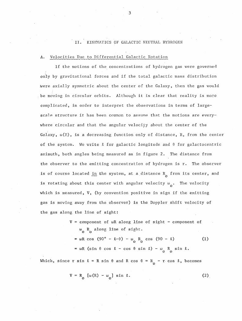
If the motions of the concentrations of hydrogen gas were governed

only by gravitational forces and if the total galactic mass distribution

were axially symmetric about the center of the Galaxy, then the gas would

be moving in circular orbits. Although it is clear that reality is more

complicated, in order to interpret the observations in terms of large-

scale structure it has been common to assume that the motions are every-

where circular and that the angular velocity about the center of the

Galaxy, w(R), is a decreasing function only of distance, R, from the center

of the system. We write E for galactic longitude and 0 for galactocentric

azimuth, both angles being measured as in figure 2. The distance from

the observer to the emitting concentration of hydrogen is r. The observer

is of course located in the system, at a distance R from its center, andO

is rotating about this center with angular velocity mo . The velocity0

which is measured, V, (by convention positive in sign if the emitting

gas is moving away from the observer) is the Doppler shift velocity of

the gas along the line of sight:

V = component of wR along line of sight - component of

a R along line of sight.O o

= wR cos (90 ° - E-6) - w R cos (90 - ) (1)O o

= wR (sin e cos k - cos 0 sin ) - w R sin 2.S0 0

Which, since r sin 2 = R sin 6 and R cos 0 = R - r cos 2, becomes0

V = Ro [w(R) - wo] sin R.0 0 (2)

This is the fundamental equation of 21-cm galactic structure analysis.

If the function R [o(R) - m ] is known, then in principle distances0 0

along the line of sight can be attributed to each measured V. It is worth

emphasizing that distances are not determined directly, but require ac-

curate knowledge of the velocity-field throughout the Galaxy.

Practical application of equation (2) raises a number of problems.

The first of these involves the accuracy with which the angular-velocity

rotation curve w(R) can be determined. Within the framework of the

assumptions of the preceding paragraph this can be determined from 21-cm

measurements for regions along the line of sight where R < RO, as follows.

For any reasonable rotation law V will vary as shown schematically in

figure 3. Consider a particular line of sight with k in the range

00 < ZI < 900. As the distance from the Sun, r, increases along this

line of sight, the distance to the galactic center at first decreases.

This corresponds to increasing w(R) and thus to increasing IVI . However,

as r increases further a point on the line of sight is reached which is

closest to the galactic center. At this "subcentral point", R = R . =mm

R sin I., and w(R) and thus IV I reach maximum values. For still larger

r, R increases so that V decreases from the value it reached at the sub-

central point. By measuring the cut-off value of IV! on a profile observed

at each longitude and attributing this "terminal velocity" to the distance

from the center, R sin JEf, corresponding to that longitude's subcentral0

point, one obtains o(R) provided R and a are known from other methods.o o

The terminal velocity, which is thus VT = R0 [w(R sin £1 ) - to] sin 2,

is in practice taken as a suitably defined point on the high velocity

edge of each profile. The linear-velocity rotation curve, giving the

circular velocity 0(R) = tR as a function of T, is then obtained using

5

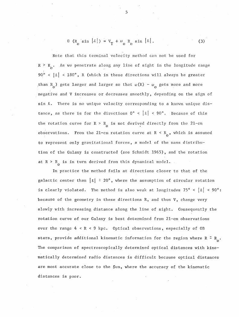
o (R sin &I) =VT + b R sin HI. (3)o T o o

Note that this terminal velocity method can not be used for

R > R . As we penetrate along any line of sight in the longitude range0

90° < [1 < 180 °, R (which in these directions will always be greater

than R ) gets larger and larger so that w(R) - w gets more and more

negative and V increases or decreases smoothly, depending on the sign of

sin Q. There is no unique velocity corresponding to a known unique dis-

tance, as there is for the directions 0 < IZ1 < 900. Because of this

the rotation curve for R > R is not derived directly from the 21-cm0

observations. From the 21-cm rotation curve at R < Ro, which is assumed

to represent only gravitational forces, a model of the mass distribu-

tion of the Galaxy is constructed (see Schmidt 1965), and the rotation

at R > R is in turn derived from this dynamical model.0

In practice the method fails at directions closer to that of the

galactic center than j1 Q 200, where the assumption of circular rotation

is clearly violated. The method is also weak at longitudes 750 < H < 90° .

because of the geometry in these directions R, and thus V, change very

slowly with increasing distance along the line of sight. Consequently the

rotation curve of our Galaxy is best determined from 21-cm observations

over the range 4< R < 9 kpc. Optical observations, especially of OB

stars, provide additional kinematic information for the region where R R .0

The comparison of spectroscopically determined optical distances with kine-

matically determined radio distances is difficult because optical distances

are most accurate close to the Sun, where the accuracy of the kinematic

distances is poor.

The rotation curve derived by Shane and Bieger-Smith (1966) from

observations in the first quadrant of galactic longitude is shown in

figure 4. We will see in the following section that the irregularities

in'. this rotation curve can be attributed to large-scale streaming motions.

Over much of the Galaxy the deviations from circular velocity are of the

order of 5% of the rotation velocities. In the central region where

R < 4 kpc the non-circular motions are on the same order as the rotation

velocities.

It is also clear from figure 4 that over much of the Galaxy 0

changes much more slowly with respect to R than would be the case for

solid body rotation. This strong differential rotation indicates a

strong increase in total mass towards the center of the galactic system.

It is sometimes useful to have available a simple analytic expres-

sion for the rotation curve freed of the perturbations of streaming

motions. The expression

20 (R) = R w(R) = 250.0 + 4.05 (10-R)-1.62 (10-R) (4a)

is a satisfactory fit to the apparent curve in figure 4. It is valid

for the region 4 < R < 10 kpc in the first quadrant of galactic longitude.

For the extrapolated region 10 < R < 14 kpc, a fit to the rotation

required by the Schmidt (1965) mass model is given by

0 (R) = R o(R) = 885.44 R-1/2 - 30000 R - 3 . (4b)

Velocities with respect to the local standard of rest, calculated

from equation (2) using the velocity-field described by equation (4),

are plotted as a function of distance from the Sun in figure 5. This

figure illustrates in more detail the points illustrated schematically

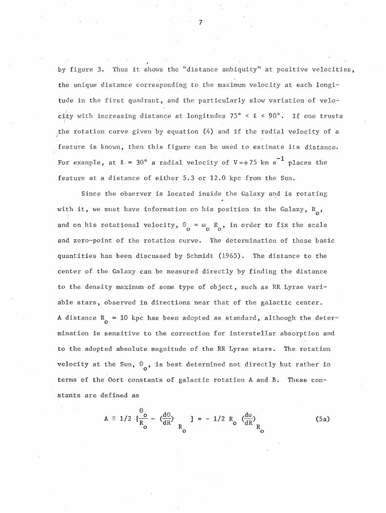
by figure 3. Thus it shows the "distance ambiquity" at positive velocities,

the unique distance corresponding to the maximum velocity at each longi-

tude in the first quadrant, and the particularly slow variation of velo-

city with increasing distance at longitudes 750 < k < 90 ° . If one trusts

/the rotation curve given by equation (4) and if the radial velocity of a

feature is known, then this figure can be used to estimate its distance.

-lFor example, at k = 30 ° a radial velocity of V=+75 km s places the

feature at a distance of either 5.3 or 12.0 kpc from the Sun.

Since the observer is located inside the Galaxy and is rotating

with it, we must have information on his position in the Galaxy, R,O0

and on his rotational velocity, 0 = c R , in order to fix the scaleS0 00

and zero-point of the rotation curve. The determination of these basic

quantities has been discussed by Schmidt (1965). The distance to the

center of the Galaxy can be measured directly by finding the distance

to the density maximum of some type of object, such as RR Lyrae vari-

able stars, observed in directions near that of the galactic center.

A distance R = 10 kpc has been adopted as standard, although the deter-0

mination is sensitive to the correction for interstellar absorption and

to the adopted absolute magnitude of the RR Lyrae stars. The rotation

velocity at the Sun, 00, is best determined not directly but rather ino

terms of the Oort constants of galactic rotation A and B. These con-

stants are defined as

0o dO d

A - 1/2 [--- ( - ) J = - 1/2 R (d) (5a)o R o dR(

0 0

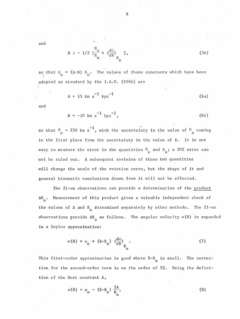
and6

B - 1/2 [0-o dO) '] (5b)o R

0

so that 0 = (A-B) R . The values of these constants which have beeno o

adopted as standard by the I.A.U. (1966) are

. - -

A = 15 km s kpc-1 (6a)

and

-1 -lB = -10 km s-1 kpc -1, (6b)

-1so that 0 = 250 km s , with the uncertainty in the value of 0 coming

o o

in the first place from the uncertainty in the value of B. It is not

easy to measure the error in the quantities 0 and R ; a 20% error cano o

not be ruled out. A subsequent revision of these two quantities

will change the scale of the rotation curve, but the shape of it and

general kinematic conclusions drawn from it will not be effected.

The 21-cm observations can provide a determination of the product

AR . Measurement of this product gives a valuable independent check ofo

the values of A and R determined separately by other methods. The 21-cmo

observations provide AR as follows. The angular velocity w(R) is expanded0

in a Taylor approximation:

dwW(R) = m + (R-R ) () . (7)

o o dRR

o

This first-order approximation is good where R-R is small. The correc-0

tion for the second-order term is on the order of 5%. Using the defini-

tion of the Oort constant A,

2Aw(R) = o - (R-Ro) 2 (8)

o o R0

so that substitution in equation (2) gives

V = -2A (R-Ro) sin 9. (9)0

Still assuming circular rotation, there is no distance ambiguity for the

terminal velocity, VT, since this velocity corresponds to R = R .= RT mmn o

sin I2. Consequently measurements of the terminal velocities give

ARo = VT [2 sin 9 (1 - sin Q )]-l. (10)

The product should be determined from observations at longitudes not too

much less than 900 in order for the assumption R R to remain valid.O

-iThe variations observed in VT, which are of the order of 5 km s and

attributed to systematic streaming motions, will introduce large errors

in AR since the denominator in equation (10) is less than 1. Neverthe-0

-1less, 21-cm determinations of AR lie in the range 135 to 150 km s ,0

consistent with the adopted values of A and Ro0

Using these values of R and 0 , the period of revolution of theo o8

local standard of rest around the galactic center is 27r R /0 = 2.5 x 10O O

years. This is only 1 or 2 per cent of the age of the galactic disk.

How structure in the disk is maintained against the shearing forces of

the strong differential rotation for times longer than one galactic

revolution has remained a puzzle.

B. Deviations from Circular Symmetry and Circular Motions

One assumption which is important in the rotation curve derivation

is the assumption that there is enough hydrogen present near the subcentral

point to actually determine the cut-off of the profile. Suppose there is

10

o0

not enough hydrogen there; then the measured terminal velocities would be

contributed by gas in a region with R > R sin I91 and thus w < w0

(R sin I9) so that the derived 0(R) would be less than the true velocity.0

In fact, the observed rotation curve plotted in figure 4 shows irregularities

in the velocities plotted against distance from the center. In the original

determination of the rotation curve by Kwee, Muller and Westerhout (1954),

this sort of irregularity was attributed to extended regions that did not

contain enough gas near the subcentral point to determine the profile cut-

off. The idea was that if there was not much gas at the subcentral point,

the observed cut-off velocity would be due to lower velocity gas at

R > R sin 94 . If this is the case, then the rotation curve should be0

drawn using the upper envelope of the observed terminal velocities. Cir-

cular motion could in this way be retained. However, Shane and Bieger-

Smith (1966) showed that the irregularities could better be attributed

to large-scale streaming motions, that is, to systematic deviations from

circular rotation. They rejected the possibility of large empty regions

because low-intensity extensions on the ends of profiles are not observed

at longitudes corresponding to the dips in the run of observed terminal

velocities. A model based on circular rotation and reproducing most

characteristics of the terminal velocities could only be constructed by

using an unacceptably artificial density distribution. In order for the

whole maximum velocity part of the profile to shift to lower velocities

there would have to be essentially no hydrogen (about a factor 100 less

than the average hydrogen density) along the whole region of the line of

-1sight within approximately 10 km s of the velocity corresponding to the

11

subcentral point. This means (as is clear from inspecting figure 5),

that regions of 4 or 5 kpc extent would have to be essentially empty of

gas, and that these regions would have to have a preferential orientation

with respect to the observer. This is implausible. The conclusion that

the observed irregularities in the run of the terminal velocities reflect

corresponding irregularities in the galactic velocity-field is an important

one.

There are other indications that the assumption of circular rotation

is less than satisfactory. Unambiguous proof of noncircular motions in

the Galaxy is given by profiles observed i the galactic plane in the

cardinal directions k = 0° , 90° and 1800. The velocities expected in

terms of circular rotation at these longitudes are illustrated in figure

5, while figure 6 shows the profiles observed. At longitudes 0 ° and

1800, all circular motions would be perpendicular to the line of sight,

and in the presence of only such motions the profiles would have one

peak symmetric with respect to zero velocity. Actually, strong radial

motions are observed. For = 900, circular motion would imply no posi-

tive velocity peak in the profile. Actually, there is a peak at V : +6

-1km s-.

Since there is no reason to expect these irregularities to be

axially symmetric, or even to have characteristic length scales of more

than a few kiloparsecs, the rotation curve illustrated by the wavy line

in figure 4 is an apparent one only, since it describes motions along one

particular locus, and not over the entire galactic plane. This locus is

not necessarily the locus of subcentral points since in the presence of

deviations from circular motion the terminal velocity does not necessarily

originate at the subcentral point. Thus it is not surprising that the

12

apparent rotation curve derived from observations of the terminal velo-

cities in the longitude quadrant - 900 < Q < 0 ° has irregularities some-

what differently placed, although of about the same amplitude. What is

more disturbing is that the unperturbed or basic rotation curve, obtained

by drawing a smooth curve through the irregular apparent one, is different

when determined for the fourth quandrant than when determined for the

first quandrant. A pair of apparent rotation curves obtained on the

two sides of the galactic center is shown in figure 7. The systematic

-1difference of about 10 km s between the two curves over the regions

30° < J1 < 530 is further evidence requiring us to accept kinematic

asymmetries on a very large scale.

Deviations from circular symmetry in our Galaxy can be demonstrated

in more detail by comparing the cut-offs on both the positive- and

negative-velocity wings of profiles observed at the corresponding longi-

tudes k and -Q. Such a comparison is shown in figure 8. The differences

in the cut-offs at corresponding longitudes are large and systematic.

The cut-offs plotted in figure 8 provide information from different

parts of the Galaxy. Although different explanations may have to be found

for each region, explanations in terms of kinematics seem more plausible

than explanations in terms of the density distribution.

These deviations from circular symmetry have important consequences

for the derivation of the galactic distribution of the neutral hydrogen.

These consequences are the subject of section III B.

C. Non-Circular Motions Predicted by the Linear Density-Wave Theory

The density-wave theory of galactic rotation has had some success

in explaining the observed velocity characteristics of the Galaxy. It

13

also provides a plausible mechanism for maintaining spiral structure against

the strong shearing forces of differential rotation. The theory is dis-

cussed in detail in a monograph by Lin and Shu (1973), but it is useful

to. briefly describe here the observable consequences of the theory.

Spiral arms are considered as waves in the theory. Stars and gas

move through the spiral arms, but since they stay longer in the arms,

the arms are density maxima. The theory provides for the maintenance of

such density waves, although it does not provide for the origin of them.

There is still little agreement on the origin of the spiral perturbation

in the first place. A density wave of spiral form is assumed to be super-

imposed as a perturbation on an axisymmetric background mass distribution.

The superimposed wave pattern moves relative to the material, with a con-

stant angular velocity Q , and thus does not follow differential rotation.~P

The resultant spiral gravitational field produces streaming motions and a

subsequent redistribution of densities which can maintain the imposed

perturbation. Although the imposed perturbation is only a few per cent

of the total mass density, the interstellar gas responds quite strongly

to it. In the linear theory, the effect of the wave on the gas and on

the stars is in phase; the effect differs only in the amplitude of the

perturbation. According to the theory the response of a particular popu-

lation of the galactic mass is determined by the population's velocity

dispersion. The interstellar hydrogen is characterized by velocity dis-

-1persions of about 5 km s whereas most of the mass is contributed by

older stars with dispersions characteristically almost an order of magni-

tude larger. Thus for the gas component the theory predicts both large

-1peculiar velocities, typically 7kin s , and a large ratio between the density

14

in the arm and interarm regions of about 3:1. Such streaming motions

or such density variations would, by themselves, have easily observable

consequences in the profiles. Since in fact such effects are superimposed

on. top of each other, separating the kinematic from the density charac-

teristics represented in the profiles is a challenging problem.

The density-wave theory relates the streaming motions and the den-

sities as follows. The deviations from circular motion are expressed

in terms of the peculiar motions, VR and V0 , taken, respectively, to be

positive in the directions of increasing radius and azimuth. These

peculiar motions are assumed to vary periodically:

VR = -aR cos (X(R, 6)),

(11)

V6 = ae sin (X(R, 6)),

where X(R, 0) = 20 - 4(R) is the phase of the superimposed spiral gravi-

tational potential, and p(R) is the radial phase function. The ampli-

tude functions of the peculiar motions are given by Lin et al. (1969) in

terms of the density contrast between the gas surface density in a unit

column perpendicular to the galactic plane through the center of a spiral

arm, a , and the gas surface density between arms, a .m:max mm

max min 2a (w(R) w- ) ,R + . p -k(R)max min

(12)

2K 1

a =a .0 4 2 R(w(R)) - w(R)w

P

15

Here m'(R) is the basic unperturbed rotation of the background mass,

such as given by equation (4). The superimposed pattern has the form

of a two-arm trailing logarithmic spiral rotating with constant angular

velocity, w , with respect to an inertial system. The epicyclic fre-P

quency, K, is defined by

2 2 R doK = (2 2(R)) (1 + R d (13)C C)) 2c,)(R) dR

The radial wavenumber of the spiral pattern is Ik(R)I where k(R) = -" dR"

The spacing between adjacent arms is I = 2y/ k(R)J.

The geometry of the spiral pattern, R (0) = R exp (-t(6-60)), is0 0

characterized by a tilt angle, t, defined as the acute angle between the

spiral and a galactocentric circle (positive in sign for trailing arms).

The tilt angle is related to the wave number by

kR 2 _= 2 . (14)k(R) -R dR -RX R tan t6 X

These equations determine the streaming motions predicted by the

first-order density-wave theory for certain assumed parameters, which

with certain restraints may be adjusted in accordance with the observa-

tions. The sense of the streaming is apparent from (12), since both

aR and ae are always positive for k(R)<0 (trailing arms) and for

w < 0(R). For our own Galaxy, the predicted radial velocity with respectp

to the local standard of rest becomes, in the presence of the density-

wave peculiar motions,

V(R,5 , 6) = V(R,) - VR cos (+6e) + V0 cos (900--6). (15)

16

Here V(r,Q) is the unperturbed basic rotation described by equation

(2). The density-wave streaming motions relative to the local standard

of rest, given by the two righthandmost terms in equation (15), are plotted

in figure 9. Indeed it is qualitatively understandable that a stretched-

out structural feature will, by its own gravitational forces, induce

streaming motions in the sense indicated. Material on the outer side

of the feature will be pulled towards it, increasing the material's

angular momentum and thus increasing its velocity in the direction of

rotation. The situation will be the other way around for material on

the inner side of such a feature.

The density-wave theory is valid over the range of the galactic

disk for which the conditions

w(R) - -< < w(R) K (16)~' 2< p2

are satisfied. The pattern speed w has been chosen by Lin et al. sop

that this range is as large as possible. At the borders of this range

are the locations of the so-called Lindblad resonances. According to

the theory the pattern ends here as a ring. Outside this range the

theory is no longer applicable, and so far it is not completely clear

what the observational consequences of these resonances would be. For

-l -l

our own Galaxy and a pattern speed of 13 km s-1 kpc -, the inner Lindblad

resonance occurs at R Z 3 kpc. It has been suggested that resonance phe-

nomena might be able to account for the large radial motions observed

in the 21-cm line near the "3-kpc arm" (Shane 1972, Simonson and Mader

1972).

17

The density-wave theory has been applied in some detail to the

interpretation of the velocity and density patterns observed in the

Milky Way. Streaming motions of the sort predicted by the theory and

illustrated by figure 6 have been observed in the gas (Burton 1966,

1971, 1972; Burton and Shane 1970; Shane 1972; Tuve and Lundsager 1972)

and in the youngest stars (Humphreys 1970, 1971, 1972). Deriving an

apparent rotation curve, using equation (15) and best-fit density-wave

parameters, results in the dashed curve labelled "model" in figure 4.

This calculated rotation curve is certainly a better fit to the one

derived from the first-quadrant observations than the one derived using

the circular rotation equation (2). The theory has also been used to

interprete observations of a few external galaxies (M101, Rogstad 1971;

M51, Mathewson et al. 1972).

III. DETERMINATION OF GALACTIC STRUCTURE

The standard overall picture of the neutral hydrogen distribution

in the Galaxy is still the one based early Dutch and Australian observa-

tions (Schmidt 1957, Westerhout 1957, Kerr 1962). This map, shown in

figure 10, was derived using the basic equation (2). We have seen that

the assumptions of axial symmetry and circular rotation inherent in this

equation are not generally valid. It now remains to be seen how this

should influence the interpretation of the standard map in figure 10,

and to discuss some of the problems involved in the derivation of

such a map.

18

A. Line Profile Characteristics Caused by Geometrical Effects

It is instructive to look in more detail at the change of V with

distance along the line of sight calculated for the simple circular rota-

tion described by equation (4). This velocity with respect to the local

standard of rest is plotted (using a full-drawn curve) against distance

from the Sun for two typical longitudes, Z=500 and £=750, in figure lla.

Two things are immediately evident from this figure. In the first

place, there are two regions on the line of sight which contribute to

each positive velocity, whereas only one region contributes to each

negative velocity. This distance ambiguity is expected in all directions

where JZJ < 90° . If the hydrogen gas is optically thin and generally

distributed throughout the Galaxy, the effect of this double-valuedness

at positive velocities (for 0 ° < Q < 90 ° ) should show up in the observa-

tions since the intensities at positive velocities should then typically

be about twice what they are at negative velocities. The actual exis-

tence of the intensity cut-off near zero velocity in the range 200 < 2 < 70°,

evident in the reference map in figure 1, indicates that on the largest

scale the hydrogen gas at these longitudes is indeed optically thin. In

the second place, figure lla shows that the velocity observed from re-

gions near the subcentral point changes relatively slowly along the line

of sight. Consequently the profiles contain, near the terminal velocity,

a contribution from an especially long path-length. This crowding in velo-

city results in the high-velocity ridge pattern, which is a striking

characteristic of the observations in the reference map.

2The number of hydrogen atoms in a column of 1 cm cross-section

dV -1per unit interval of velocity is nH (h-j) , where nHis the density

19

of hydrogen atoms per cubic centimeter. Assuming that the hydrogen is

more or less evenly distributed, the relative contribution to the pro-

files at each velocity is determined by the rate of change of the velo-

city with distance. This is illustrated by figure llb. Here the change

dVof velocity with distance from the Sun, d , summed at positive velocities

where there is the distance ambiquity between the near and the far side of

the subcentral point, is plotted against velocity. The vertical scale is

dV dVr , but, since intensities at velocities at which d is small will be

proportionately enhanced on the profiles, the vertical scale can be inter-

preted as an intensity scale. Thus the plots in figure lb can be con-

sidered schematic line profiles.

The full-drawn curves in figure 11 are calculated for simple cir-

cular rotation. The dashed curves in the figure, however, are calculated

for a rotation law in which large-scale streaming motions are present.

At this stage it is not important that the rotation law used is one de-

rived using density-wave theory kinematics and illustrated in figure 4.

What is important is that in the presence of deviations from circular

motion, the variation of V along the line of sight will not be as regular

as in the circular rotation case but will show the sort of structure

illustrated in figure lla. Irregularities in the plot of V against r

will show up as structure in the schematic profile constructed from the

dV$r against r relation.

Theoretical line profiles which represent the geometrical effects

in a more realistic way can be calculated assuming a rotation law and

a completely uniform hydrogen distribution. Such profiles are shown in

figure llc. The full-drawn profiles are calculated for the circular

rotation described by equation (4), for 1 = 500 and p = 750. These

20

calculated profiles illustrate that structure in the observed profiles

is to be expected even for a structureless distribution of hydrogen

throughout the Galaxy. The cut-off near zero velocity, due to the fact

that two regions contribute to positive velocities, and the enhanced

intensities near the maximum velocity, due to the crowding in velocity

near the subcentral point, are geometrical effects which are model

independent in the sense that structure of this sort would be present

in the profiles for any reasonable rotation law and density distribution.

Obviously, this sort of profile structure must be satisfactorily accounted

for in the subsequent analysis of profiles and not attributed to spurious

characteristics of the hydrogen distribution. Although there are numerous

cases in the literature where this has not been done, it should not be

too difficult to account for the model-independent effects.

Accounting for the effects of systematic streaming motions is a

different matter, however. The dashed-line profiles in figure llc were

calculated using the density-wave theory velocity-field illustrated

by figure lla and, again, a completely uniform hydrogen distribution.

The profiles show the model-independent effects, but these effects are

now superimposed on the geometrical effects attributable to deviations

from circular rotation. The dashed-line profiles illustrate the effic-

-liency with which systematic streaming motions of about 5 km s amplitude

will distort the observations; it would require large density differences

to achieve intensity differences equivalent to those obtained by syste-

-imatic streaming motions of only a few km s . The observed profiles are

included in figure llc, as dots, in order to show that the structure in

the observed profiles is of the same magnitude as the structure in the

calculated profiles.

21

B. The Kinematic Distribution of the Neutral Hydrogen

It is important to emphasize that profiles are more sensitive to

small variations in the streaming motions than to even substantial

variations in the hydrogen density (Burton 1971, 1972; Tuve and

Lundsager 1972). Line profiles are sensitive to the velocity-field be-

cause what is observed is the amount of hydrogen per unit velocity. In

the presence of streaming motions, there will be regions on the line of

sight where the radial velocity changes relatively slowly with increasing

distance from the Sun. The relative contribution to the observed profiles

from these regions where dV dr is small will be enhanced. Irregulari-

ties in the velocities are themselves sufficient to cause the appearance

in the profiles of structure which has generally been interpreted in

terms of density concentrations on galactic structure maps derived assum-

ing purely circular rotation.

In order to exploit the fact that line profiles are very sensitive

to velocity variations, we can assume for the sake of the argument that

all structure in the profiles has a kinematic origin. By adjusting the

line-of-sight streaming motions in a model, but maintaining a uniform

density and temperature distribution, any profile can be reproduced to

within a scale factor. This method of perturbing the line-of-sight velo-

city field, illustrated in figure 12, involves fitting model profiles to

observed profiles by perturbing the line-of-sight velocity field from the

basic circular-rotation velocity field described by equation (4). The

difference between the perturbed and the basic line-of-sight velocity

fields, V - V , gives information on the spatial distribution of thep o

22

streaming motions. Application of the method to profiles observed in

the galactic plane results in the distribution of the streaming parameter

V - V shown in figure 13. It is clear from this figure that thep o

observations are satisfactorily reproduced with line-of-sight streaming-1

amplitudes of the order of 7 km s . This amplitude is about 3% of the

velocity of rotation about the galactic center. The sense and magnitude

of the kinematic variations are consistent with gas motions observed in a

number of regions and with motions predicted by the density-wave theory.

The spatial distribution of V - V, provided by the procedure, is a mea-p o

sure which can be compared with optically derived velocity residuals, using

optical distances. Optical observations of HII regions, supergiants and

Cepheids show streaming motions similar in amplitude and spatial distri-

bution to those derived from the hydrogen observations.

The kinematic approach outlined here is discussed in more detail by

Burton (1972) and by Burton and Bania (1973). The detailed interpreta-

tion of a map such as the one in figure 13 requires the adoption of a

theory relating the velocity and density fields, since it is clear that

in fact fluctuations in velocity and in density will accompany each other.

In any case, the approach serves to emphasize the extreme sensitivity of

the observations to streaming motions.

C. The Model-Making Appraoch to the Derivation of the Large-ScaleStructure

Because streaming motions and density variations will generally be

associated, attempts to derive the spatial distribution of the gas should

be based on simultaneously derived solutions for the galactic velocity-

field. We have seen that even slight variations in local velocity condi-

tions can lead to substantial variations in the observed profiles. It

23

is necessary to account for the consequences of both the adopted velocity-

field and density distribution when deriving the large-scale structure.

A good way to do this is to calculate model line profiles whenever one

produces a map of the galactic structure*. These line profiles would of

course contain the effects discussed in section III A inherent in the

overall geometry and in the particular velocity-field adopted. It would

be very difficult to account for these effects otherwise. Once it is

established that the structure map is reasonable in the sense of the com-

parison of the model profiles with the observations, the map can furthe

be judged in terms of the reasonableness of the adopted velocity-field

and resultant density distribution.

Figures 14 and 15 show velocity-longitude contour maps constructed

from model line profiles. These maps can be compared with the observed

contour map in figure 1. The model in figure 14 was constructed using

a velocity-field of the type predicted by the density-wave theory and

described by equation (15). The parameters in the density-wave theory

formulation were adjusted so that the model contour map agrees as well

as possible with the map in figure 1. The resultant streaming amplitudes-l

in this model vary between 3 and 8 km s , the arm-interarm density

contrast is typically 3:1 and the tilt of the spiral pattern is about 70.

The map in figure 15 illustrates some of the failures of kinematic

models based on circular rotation. This map was constructed using the

same density distribution and the same spiral pattern as in the figure 14

model, but using only the basic rotation of equations (2) and (4), without

the density-wave theory perturbation. The different appearance between

* A procedure for calculating model line profiles has been outlined byBurton (1971).

24

the models in figures 14 and 15 is due entirely to the difference in the

velocity-fields. It is clear that the second model is a poorer fit to

the'observations.

Figure 16 illustrates the approach in more detail for the interior

portion of the Galaxy between 9 = 400 and k = 90 ° . The figure is a

composite consisting of the observed velocity-longitude contour map

(figure 16a), the model contour map which is a best fit to the observa-

tions (figure 16b) and the spatial map (figure 16c) illustrating the

density distribution used in deriving the model.

The model in figure 16, which is based on density-wave kinematics,

is similar to the one in figure 14 in most respects. The fit of the

model to the observations is judged by comparing the maps in figures

16a and 16b. The strong intensities near the terminal velocities, the

cut-off in intensities near zero velocity, and the enhanced intensities

between k Z 65 ° and 850 are interpreted in terms of the model-independent

effects discussed in section III A. The density-wave theory has been

able to account for the run of terminal velocities with longitude, as

well as the general appearance of the observations associated with the

Sagittarius spiral arm, which is seen tangentially at ~ 50 ° .

Figure 16c illustrates the space-density distribution which was

used as input in deriving the contour map in figure 16b. The shaded

part of figure 16c is the region where the density is above average; as

has been stressed, the exact density distribution is only important in

the model in that it determines the streaming amplitudes through the

equations of section II C. The borders of the shaded regions in figure 16c

are the loci of maximum 1V0 and the loci of VR = 0. In spite of the very

25

simple spatial distribution input, the resulting agreement with the

observations is rather detailed when viewed in the observed velocity

space.

D.' Some Remarks on the Spiral Structure of the Galaxy

It is clear from figure lic that any deviations from the adopted

-1rotation law of only 1 or 2 km s , which are systematic over a few

degrees on the sky, will probably cause serious errors in the interpre-

tation of the profiles. Since the kinematics dominate the appearance

of the profiles, interpretation of the structure observed in the pro-

files in terms of a map of the density distribution requires very

accurate knowledge of the velocity-field throughout the Galaxy. How-

ever, the velocity-field is only directly measured along a restricted

region near the locus of subcentral points. At the same time it is also

obvious that structure in the temperature distribution will also result

in structure in the observed profiles. Consequently it is necessary

to know the temperature distribution on a large scale. Maps of the

hydrogen distribution have generally been based on the further assump-

tions that the temperature of the gas is constant and that the optical

depth is low. Although there is abundant evidence that these assump-

tions are not generally valid, they have been necessary in order for

the analysis to proceed.

We saw in the preceding section that streaming motions of the sort

known to exist are themselves capable of producing structure in the pro-

files of the same sort which is observed. This implies that the inter-

pretation of 21-cm profiles in terms of a map of the density distribution

26

on a galactic scale is, at best, difficult. Even if the peaks in the

profiles are correlated with density concentrations, it will be difficult

to account for the profile distortions caused by streaming motions and

temperature variations in terms of the hydrogen density distribution.

Only in the special case of gas concentrations with no systematic

streaming, free from the shearing effects of differential rotation, with

constant temperature throughout, and isolated from the model-independent

geometrical effects can the relative heights or peaks and valleys in the

profiles be interpreted directly in terms of a cdensity contrast between

"cloud" and "intercloud" regions. Similarly only in such a situation will

the measured dispersion be a direct indication of the random cloud velo-

cities. Although such a situation may pertain locally at large distances

from the galactic plane, it certainly does not pertain in the plane itself.

In fact, it is not clear if a particular peak in a line pro-

file owes its characteristics to streaming motions, to a density concen-

tration, or to a variation in temperature. Although it is certain that

fluctuations in the velocity, density and temperature will accompany one

another, the interstellar hydrogen is embedded in such a complicated en-

vironment that it does not seem possible to determine, directly from

the observations, the relative importance of the variables for each

peak or valley in a profile. Near the galactic plane this very com-

plicated environment includes HII regions, supernovae and their expand-

ing shells, regions of star formation, gravitational effects from mass

concentrations, and the largly unknown effects of magnetic fields

which are probably coupled to the neutral gas by collisions between

27

the plasma component and the neutral one. Each of these mechanisms

can produce differences in the motions, densities and temperatures on

a scale large enough to effect the appearance of the profiles and thus

of. the subsequent map. This means that hydrogen density variations in

the galactic plane cannot be determined with any accuracy directly from

observations. Similarly it is not possible to determine the true velo-

city dispersion from observations in the plane.

Irregularities in the velocities are themselves sufficient to

cause the appearance of "spiral arms" on maps derived assuming circular

rotation. We saw that irregularities in the velocity-field are observed

along the locus of subcentral points. If distances are derived using

a mean rotation curve such as the curve described by equation (4), then

there will be some intensities observed at velocities higher than the

rotation velocities. In preparing the map in figure 10, hydrogen con-

tributing such intensities was distributed uniformly over 2 kpc (2.4

kpc if corrected from the old value R = 8.2 kpc to R = 10 kpc) of0 0

line of sight, situated symmetrically with respect to the subcentral

point distance (Schmidt 1957).

The region near the subcentral points in the classic map gets rela-

tively low weight also for the following reason. In preparing the map,

the distance ambiquity problem for R < R was approached by assuming0

that the hydrogen layer had a constant thickness. By measuring the

distribution in latitude at each velocity an attempt was made to separate

the material on the near side of the subcentral point, at a distance

rl from the Sun, from the material on the far side of the subcentral

point, at a distance r 2 where it would substend a smaller angle. For

r2the region < 1.8, which is defined on the map in figure 10 by heavy

rl

28

lines, the method was not considered accurate enough to allow a separa-

tion. For lack of any other information, the contributions at r and

r2 were taken equal. The resulting regularity in the region where

rl. < 1.8 is therefore probably fortuitous.

Hydrogen associated with small scale regions with peculiar kine-

matics, such as expanding associations, could also have influenced the

appearance of figure 10. Clube (1967) suggested that the unique kinematics

of the local system of luminous B stars within 400 pc of the Sun known

as Gould's Belt is sufficient to cause the appearance of a spurious

structure on a map of the large-scale structure drawn using a velocity-

field described by simple circular rotation.

The map of the large-scale hydrogen distribution in figure 10 has

to be considered in these terms. The apparent regularity near the locus

of subcentral points has low weight. Some other apparently regular

features of the map may be spurious. Most of the assumptions upon which

the validity of the fundamental equation depends are not strictly

correct; even small deviations from the assumed situation can result

in substantial errors in the map. However, it should be added that in

many cases, even if a peak in a profile owes its prominence to streaming

motions, this streaming motion can be seen as a perturbation on the

basic rotation described by equation (4). Consequently the distance

assigned to peaks using the basic rotation may be correct to the first

order.

Even with these reservations, it seems safe to conclude that 21-cm

observations do indicate structure on a large-scale in the galactic plane,

although it is not immediately clear whether this structure owes its

29

prominence to velocity, de nsity or temperature fluctuations. In some

cases the structure defines extended regions of some kiloparsecs length.

These extended regions are situated, roughly, along galactocentric arcs.

But, I wonder if we would call this structure s al structure if we had

no knowledge of other galaxies. This is not to imply that spiral struc-

ture does not exist in our Galaxy. After all, we do have knowledge of

other galaxies and spiral structure is present to some degree in almost

all galaxies with sufficient gas in a disk distribuiton. Although an

examination of a number of other galaxies in photographs such as those

in the Hubble Atlas of Galaxies shows that the structure is more often

than not very irregular, in a number of galaxies a general spiral

"grand design" emerges from a more or less tangled background structure.

Galaxies with such a grand design can be expected to provide much of the

information necessary for a confrontation with theories of spiral

structure. But it does not seem to me that the 21-cm observations have

demonstrated that our Galaxy does, or does not, belong to the galaxies

which display such a grand design.

The problem of the origin and maintenance of spiral structure in

galaxies is obviously of fundamental importance. To confront theories

of spiral structure, observations are necessary which w-ill provide answers

to questions which are so far not satisfactorily answered for our own

Galaxy. For our own Galaxy we do not have complete answers to the follow-

ing questions. Does our Galaxy exhibit a "grand design" of spiral struc-

ture? If our Galaxy does have more or less regular arms, are these arms

trailing or winding with respect to galactic rotation? What pitch angle

30

and what spacing between arms characterize the structure? What is the

density distribution across an arm? What are the motions of the gas

between arms? What are the motions and distribution of the gas relative

to the stars? Solutions to these spiral structure problems require that

distances be determined with an accuracy substantially better than the

characteristic width of a spiral feature. This might be 500 pc.

The weakness of our answers to these questions is due, more than

to anything else, to our vantage point within the Galaxy. Our vantage

point for observing other galaxies is better. It appears that many

of the problems which, according to the plans of a decade ago, were to

be solved for the Milky Way system using 21-cm methods, can now better

be approached through investigations of other galaxies. This requires

line receivers of great sensitivity and telescopes of high resolution.

At the same time the Milky Way problems should be investigated using

all the material which can be made available. The picture of the Galaxy

which will emerge will be a synthesis of information from a variety of

studies, which might inlcude: 0- and B-type stars and their associations,

M-type supergiants, long-period Cepheid variables, the distribution of

optical and radio polarization vectors, the distribution of the continuum

background radiation, the integrated properties of 21-cm profiles, the

information contained in the latitude variations of 21-cm parameters,

optical and radio studies of HII regions, and optical and radio studies

of absorption lines.

There is also much which can be, and has been, learned about the

neutral hydrogen distribution with less accurate distances. This is

discussed in the following sections.

31

IV. THE NEUTRAL HYDROGEN LAYER

Observations of the hydrogen distribution in the z-direction

(perpendicular to the galactic plane) have been a source of information

for which accurate distances are not necessary. These observations have

shown that the gas is confined to a thin and quite flat layer at dis-

tances R < R . In the outer parts of the Galaxy the layer is thicker0

than in the inner parts and is systematically distorted from the plane

defined by b = 0.

This layer can be studied at distances R < R by measuring at each0

longitude the distribution in latitude of the intensities observed near

the terminal velocity. At the terminal velocity there is no distance

ambiquity so the linear thickness of the layer can be measured. The

deviation of the center of mass from the galactic plane defined by b = 0°

can also be measured. Studies of this sort have shown that, although

structure is present, this structure is confined to a remarkably thin

and flat layer at distances from the center less than R ~ R . The average0

full thickness of the layer to half-density points is about 220 pc. This

thickness depends on the subcentral point distances which in turn depend

geometrically on the distance scale of the whole Galaxy. In the original

thickness determination by Schmidt (1957), R = 8.2 kpc was used. Al-0

though subsequent determinations of the layer thickness using telescopes

of higher resolution have shown the angular thickness to be somewhat smaller

than in the original determination, the revision of the distance scale

to R = 10 kpc allows the characteristic thickness of about 220 pc to be0

retained. Within the circle R = R the deviation of the center of masso

32

of this layer from the "galactic equator defined by b = 0 ° is less than

30 pc. These quantities can be compared with the diameter of the layer,

which is about 30 kpc.

From the general flatness of the central layer inside the solar

distance it is evident that systematic motions in the z-direction must

'-ibe smaller than a few km s . The random gas velocities in the z-direc-

tion must increase toward the galactic center in order to dynamically

maintain the constant layer thickness against the total mass density,

which increases strongly toward the center of the Galaxy. In order to

maintain constant thickness the velocity dispersion in the z-direction8Kz

should increase proportionally to a', the derivative near the galactic

plane of the gravitational force in the z--direction. This derivative

increases by a factor of about 3 between R = 10 kpc and R = 4 kpc. The

average random motion in the z--direction at R = 100 pc might be as high

-las 50 km s -. We saw in the preceding sections that the actual random

gas velocities are difficult to measure near the galactic plane; however

there is some evidence that the dispersion increases with decreasing

R. Observations of the dispersion will be easier in other galaxies when

adequate equipment is available.

The density of the neutral hydrogen gas remains roughly constant

over the entire galactic disk, again in contrast to the density of stars,

comprising the bulk of the mass of the Galaxy, which increases strongly

toward the center.

Although the average thickness of the layer does not vary much in

the part of the Galaxy with R < Ro, this is not to imply that the layer

33

is symmetric with respect to b = 00, either in temperature or velocity

characteristics. In particular, velocity shearing motions are commonly

observed, but not completely understood.

The characteristics of the central layer in the transition region

near R = R are difficult to measure because of the superposition ofo

local gas on the parts of all profiles near zero velocity, and because

of very poor distance determinations near R = R .0

At distances R > R the central gas layer is not centered at b = 0 ° .

In several cases features extend to a height of several kiloparsecs in

the direction perpendicular to the plane. These extensions seem to be

associated with the spiral structure in the plane. This association

with the structure in the plane is evident in the first place because

the extensions occur at the same velocity interval as the structure

near b = 00. There is presumably no ambiquity in this velocity associa-

tion because of the one-to-one correspondence of velocity to distance in

the outer regions. (Primarily because of this one-to-one correspondence

the parts of the profiles contributed by the outer regions of the Galaxy

are simpler in appearance than the parts contributed by the interior

regions, although this of course does not imply that the physical structure

is simpler.) The example ofa-high-z extension in figure 17 is at a height

of z = 3.5 kpc at b = 100. The derivation of this height requires that

the distance to the arm in the plane is known. However even an error

of 3 kpc in this distance will result in an error of only 0.5 kpc in the

z-height.

The high-z extensions remain poorly understood. It is natural

to ask how the material reached such large distances into the halo, and

34

once there how it is maintained in the rather narrow velocity slot cor-

responding to the spiral feature in the plane. It is also difficult to

understand how these extensions have preserved their small internal velo-

city dispersions and not evaporated into the halo. This is all the more

enigmatic since it is conceivable that a violent event or events led to

the large z-distances in the first place. Oort (1970) has suggested that

if the extensions are expelled from the central layer, explosions such

as those observed by Hindman (1967) in the Small Magellanic Cloud could be

a possible source of energy. It seems clear that the material would

return to the central layer under gravitational attraction on a short

time scale of about 107 years. The inference is that some replenishment

or maintenance mechanism is necessary, since it does not seem reasonable

to assume that this rather general phenomenon has come about so recently.

Although the observations of these extensions are still scanty, it

is known that the extensions show strong asymmetries with respect to the

central layer. In the first quadrant the extensions are primarily to

positive latitudes. The example in figure 17 shows no corresponding

feature on the negative latitude side of the galactic equator. This ex-

tension is consistent with a general warping of the central layer. This

warping is such that the centroid of maximum neutral hydrogen density is

located at positive latitudes in the first longitude quadrant, while it

is found at negative latitudes in the fourth quadrant. Figure 18 is a

relief map showing the position of the centroid of the hydrogen distribu-

tion with respect to the plane b = 00. It is not known to what extent,

if any, the total galactic mass participates in this warping. Figure 18

35

serves as a reminder that the structural properties derived from observa-

tions at one latitude, such as the kinematic properties represented in

figure 13, may not be representative of the properties at adjacent lati-

tudes.

There have been several theoretical attempts to explain the curious

warping of the hydrogen layer. These attempts are reviewed by Hunter

and Toomre (1969). Realizing that the Large Magellanic Cloud is at the

galactocentric longitude corresponding to the maximum downward bending.

Burke (1957) and Kerr (1957) suggested that the bending might be a tidal

distortion by the Magellanic Clouds. Although these authors doubted if

the Clouds could be massive enough to account for the distortion, others

recently reexamined the suggestion and concluded that resonance could build

up adequate effects if (and this is a stringent requirement) the Large

Magellanic Cloud has remained in a closed orbit around the Galaxy for

about 15 revolutions. Habing and Visser (1967) and Hunter and Toomre

(1969) also favor a tidal distortion, but one which arose from a single

close transit of the Large Cloud. Hunter and Toomre's model requires a

passage of the Large Cloud at a distance of about 20 kpc from the center

of the Galaxy. It has also been suggested that close passage of the Cloud

might be responsible for some spiral-like structure in the Galaxy. Alter-

native interpretations of the observed warping have been given by Kahn and

Woltjer (1959), who suggested that the distortion might be due to a flow

of intergalactic gas past the Galaxy, and by Lynden-Bell (1965), who con-

sidered a free oscillation mode of the spinning galactic disk.

Although most of the hydrogen is confined to the central layer, it

appears that there is a diffuse and structureless component of hydrogen

36

extending at least several hundred parsecs beyond the main concentra-

tions. The distribution of densities in the central layer in the direc-

tion perpendicular to the galactic plane is approximately Gaussian.

However, the distribution does deviate from Gaussian in the form of

low-intensity wings extending to higher z-distances. A decomposition

of individual line profiles into Gaussian components by Shane (see Oort,

1962) has shown evidence for a background envelope of hydrogen with a

-ilarger characteristic velocity dispersion ( 11 km s -1) and a larger

thickness in latitude to half-density points (N 700 pc) than exhibited

by the more intense structure in the central layer. Emission from this

diffuse background shows a much smoother distribution than that shown by

the main concentrations of hydrogen nearer the galactic equator. Shane

-3finds at R = 7 kpc a density of 0.01 atoms cm-3 at a height of z = 600 pc.

This density is about 4% of the density in the plane.

V. NEUTRAL HYDROGEN IN THE GALACTIC NUCLEUS

The nuclei of large galaxies commonly show signs of eruptive acti-

vity. A growing body of evidence suggests that an understanding of the

phenomena occurring in galactic nuclei is necessary for an understanding

of phenomena observed throughout galaxies. The neutral hydrogen in the

central region of our own Galaxy has been studied in detail, and although

so far no complete dynamical explanation of the observations has been

given, a rather clear picture of the kinematics of the central region has

emerged.

The reference map in figure 19 shows 21-cm observations made in

the galactic plane in the directions -60 3 _< 160. What has been called

37

the "nuclear disk" appears in this map as the narrow ridge of intensi-

ties between k = 0 ° and £ = 1?5, extending through negative velocities

to about -210 km s 1. There is a similar ridge on the other side of the

galactic center between k = 0 ° and 9 = +175, at positive velocities,

which although somewhat confused with other material is clearly symmet-

ric with the ridge at negative velocities. This symmetry both with

respect to the direction of the center and with respect to zero velocity

strongly suggests that the intensities originate in the central region.

The angular extent of the disk implies, adopting R = 10 kpc, a radius

of 'about 260 pc.

That the velocities in the disk are rotational velocities seems

certain in view of the fact that no sign of non-circular motions attri-

butable to the disk is evident at Z = 0o, either in emission or in

absorption. The rotational velocity increases very rapidly going out

from the center.

The outer boundary of the disk is quite sharp. The map in figure

19 illustrates the structureless appearance of the nuclear disk, especi-

ally for the negative velocities which are uncontaminated by foreground

or background emission. This smooth appearance, together with the lack

of radial motions, implies that the disk has not been disrupted by violent

events in the nucleus.

The nuclear disk extends to k Z + 175. Between £ = -325 and -425,

-lcentered at V -240 km s , there is another concentration which also

has a symmetric counterpart at positive longitudes and positive velocities.

This "nuclear ring" also has very sharp boundaries. In particular, the

intensities at the uncontaminated negative velocities show that the region

38

between the nuclear disk and the ring, at k -3 ° , contains relatively

little neutral hydrogen. As is the case with the disk, the asymmetry

-lwith respect to both k = 00 and V = 0 km s-1 imply that the ring is

concentric with the Galaxy. The radius of the ring is about 750 pc,

and there appear to be only rotational motions within it.

Rougoor and Oort (1960, see also Oort 1971) have derived the mass

density in the nuclear region of the Galaxy, assuming that the motions

in the disk and ring are governed by gravitation only. They showed that

the velocities observed are approximately the same as Lhe velocities which

on& would expect if the mass distribution in the nuclear region of our

Galaxy would be similar to that inferred for the Andromeda galaxy from

the distribution of light. Thus 21-cm observations have given information

on the galactic rotation curve not only for the region R > 4 kpc but

also for the region R < 750 pc.

From the angle it subtends in latitude, the linear thickness of

the disk between half-density surfaces is estimated to be less than

100 pc at distances closer to the center than about 300 pc but about

230 pc in the outer parts of the disk. The density of observed neutral

-3hydrogen averages about 0.3 atoms cm-3 and is remarkable constant over

the entire disk. Although the total amount of neutral hydrogen observed

6within 750 pc is roughly 4 x 10 , the total amount of hydrogen must be

much larger since much of it must be in the form of unobserved hydrogen

molecules. The total mass within 750 pc, presumably due for the most

part to old and well mixed population II objects, was estimated by

10Rougoor and 0ort to be 2 x 10 M . The ratio of neutral hydrogen mass

to total mass is thus much less in the nuclear region than elsewhere in

the Galaxy.

39

VI. RADIAL MOTIONS IN THE CENTRAL REGION

So far we have discussed regions where the deviations from cir-

cular motion are less than a few per cent of the rotational velocities.

The situation is fundamentally different in the region outside the nuclear

disk, but inside R - 1/3 R , where non-circular motions of the same order0

as the rotational velocities are observed.

One of the most regular 21-cm features observed is the expanding

"3-kpc arm" (Rougoor and Oort, 1960; Rougoor, 1964). This feature is

evident in the figure 19 reference map as the ridge of intensities ex-

-itending from k = -6 ° at V --80 km s -, across the Sun-center line

-1S= 0 ° at V - -53 kml s , and blending into other hydrogen at k 5 ° .

-lThere is strong absorption at Z = 00, V = -53 km s -, indicating that

this branch of the arm is located between the Sun and the central con-

tinuum source Sagittarius A. The negative radial velocity of the absorp-

tion dip indicates that the feature has a net expansion away from the

center. Because of this expansion motion, the distance scale of the arm

can not be measured by the kinematic procedure of section II A. Instead,

the distance scale of the feature has been determined geometrically.

The feature can be traced to k ~ -220, where it is seen tangentially.

Here R = R sin 220 = 3.0 kpc if R = 8.2 kpc (hence the feature's name)o o

or 3.7 kpc if R = 10 kpc. Admittedly, the longitude at which the feature0

becomes tangential to the line-of-sight is not very easy to determine.

This is nevertheless the only point on the arm at which a distance can

be estimated. Its distance from the center at 1 = 00 is therefore un-

certain except that it must pass between the Sun and the center.

40

Considering now the positive velocities, we see at k = 0 ° inten-

-lsities at velocities up to about +190 km s -1. There is no appreciable

absorption at the high velocities, implying that this gas is located on

the far side of the central source and expanding away from it. There

are a number of different features evident at positive velocities. The

distances to these features, and their interconnections, are highly

hypothetical because of the lack of distance criteria.

Besides the gas in the plane, there also appears to be considerable

gas both above and below the galactic plane which is also moving in a

manner forbidden in terms of circular motion (Shane, see Oort 1966; van

der Kruit 1970). Although there is no satisfactory way to measure the

distance of this gas, the observations suggest that it is moving away

from the galactic center in two roughly opposite directions. The mass

of the neutral hydrogen involved in these motions is of the order of 106

-1M . One of the most prominent concentrations has a velocity of -130 km s0

at k = 0 ° and a mean latitude of -2°5. One plausible interpretation of

these observations, suggested by Oort (1966) and worked out by van der

Kruit (1971), involves gas ejected from the galactic nucleus with a high

velocity and at an angle with respect to the galactic plane. The angle

under which the ejection took place, 250 to 300, would have allowed the

nuclear disk to survive. According to this model, the material, which

-lhas been ejected with velocities of about 600 km s 1, would return to

the galactic plane between 3 and 5 kpc from the center, where the expan-

sion would be braked by the central gas layer. In this way, one could

account for the velocity structure of the 3-kpc arm in terms of the low

angular momentum of this ejected gas.

41

Other models for .the motions will undoubtedly be considered in the

future. In particular, the roles of hydrodynamic and magnetic forces

in the nuclear region are unknown. It is also conceivable that gravita-

tional resonance mechanisms, predicted by the density--wave theory, could

produce effects similar to those observed (Shane 1972, Simonson and Mader

1972). In addition to the 21-cm data, interpretations of the central

region will have to also account for the abundance of molecules, such

as OH and H2CO , which is high relative to other regions of the Galaxy.

In particular, it is not clear how molecular formation can take place

efficiently in the presence of the observed violent motions.

To summarize, it is not clear what mechanism is responsible for

the motions observed in the central regions, nor whether only one

type of mechanism is responsible for all these motions. It is also not

clear if the motions we observe are transient and perhaps rare pehnomena,

or if on the other hand we are observing a permanent flow of gas. The

flux involved in the gas flow is of the order of 1 or 2 solar masses per

year. If the flow is a steady phenomenon a mechanism for a circulation

of gas through the center is necessary. What is clear, in view of rapidly

accumulating evidence, is that an understanding of the activity in the

nuclei of galaxies is of utmost importance.

42

Burke, B. F. 1957 Astr. J., 62, 90.

Burton, W. B. 1966, Bul. Astr. Inst. Netherl., 1 ,247.

Burton, W. B. 1970a, Astr. Astrophls. Suppl., 2, 261.

Burton, W. B. 1970b, Astr. Astro hys. Suppl., 2, 291.

Burton, W. B. 1971, Astr. Astrophys., 10, 76.

Burton, W. B. 1972, Astr. Astrophys., in press.

Burton, W. B., Bania, T. M. 1973, in preparation.

Burton, W. B., Shane, W. W. 1970, The Spiral Structure of our Galaxy,

397-414, (Becker, W., Contoporulos, G., eds., Dordrecht).

Clube, S. V. M. 1967, The Obscrvatory, 87, 140.

Dieter, N. H. 1972, Astr. Astrophys. Suppl-., 5, 21.

Gum, C. S., Kerr, F. J., Westerhout, G. 1960, Monthl y Notices Roy. Astr.

Soc., 121, 132.

Habing, H. J., Visser, H. C. D. 1967, Radio Astronomy and the Galactic

S ystem, 159-160, (van Woerden, H., ed., London).

Henderson, A. P. 1967, Thesis, University of Maryland.

Hindman, J. V. 1967, Aust. J. Phys., 20, 147.

Hindman, J. V., Kerr, F. J. 1970, Aust. J. Phys. Astrophys. Suppl.,

18, 43.

Humphreys, R. M. 1970, Astr. J., 75, 602.

Humphreys, R. M. 1971, Astrophys. J., 163, L111.

Humphreys, R. M. 1972,

Hunter, C., Toomre, A. 1969, Astrophys. J., 155, 747.

I.A.U. 1966, Trans. I.A.U., 12B, 314-316.

Kahn, F. D., and Woltjer, L. 1959, Astrophys. J., 130, 705.

Kerr, F. J. 1957, Astr. J., 62, 93.

Kerr, F. J. 1962, Mon. Not. Roy. A.str. Soc., 123, 327.

43

Kerr, F. J. 1968, Stars and Stellar Systems, 7, 575-622, (Middlehurst,

B. M., Aller, L. H., eds., Chicago).

Kerr, F. J. 1969a, Ann. Rev. Astr. Astrophys., 7, 39.

Kerr, F. J. 1969b, Aust. J. Phys. Astrophys. Suppl., 9, 1.

Kerr, F. J., Hindman, J. V. 1970, Aust. J. Phys. Astrophys. Suppl. 18, 1.

Kerr, F. J. and Vallak, R. 1967, Aust. J. Phys. Astrophys. Suppl., 3, 1.

Kruit, P. C. van der 1970, Astr. Astrophys., 4, 462.

Kruit, P. C. van der 1971, Astr. Astrophys., 13, 405.

Kwee, K. K., Muller, C. A., Westerhout, G. 1954, Bull. Astr. Inst. Netherl.,

12, 117.

Lin, C. C., Shu, F. H. 1973, Monograph on the Density-Wave Theory, in

preparation.

Lin, C. C., Yuan, C., Shu, F. H. 1969, Astrophys. J., 155, 721.

Lindblad, P. O. 1966, Bull. Astr. Inst. Netherl. Suppl., 1, 177.

Lynden-Bell, D. 1965, Monthly Notices Roy. Astr. Soc., 129, 299.

Mathewson, D. S., Kruit, P. C. van der, Brown, W. N. 1972, Astr.

Astrophys., 17, 468.

Oort, J. H. 1962, Interstellar Matter in Galaxies, 71-77, (Woltjer, L.,

ed., New York).

Oort, J. H. 1966, Non-stable Phenomena in Galaxies, 41-45, Arakeljan, M.,

ed., Yerevan).

Oort, J. H. 1970, Astr. Astrophys. 7, 381.

Oort, J. H. 1971, Nuclei of Galaxies, 321-344, (O'Connell, D. J. K., ed., Amsterdam).

Oort, J. H., Kerr, F. J., Westerhout, G. 1958, Monthly Notices Roy. Astr. Soc.,

118, 379.

Rogstad, D. S. 1971, Astr. Astrophys., 13, 108.

Rougoor, G. W. 1964, Bull. Astr. Inst. Netherl., 17, 381.

Rougoor, G. W., Oort, J. H. 1960, Proc. Nat. Acad. Sci., 46, 1.

Schmidt, M. 1957, Bull. Astr. Inst. Netherl., 13, 247.

44

Schmidt, 1. 1965, Stars and Stellar Systems, 5, 513-530 (Blaauw, A.,

Schmidt, M., eds., Chicago).

Shane, W. W. 1971a, Astr. Astrophys. Supp 1., 4, 1.

Shane, W. W. 1971b, Astr. Astrop hys. Suppl., 5, 21.

Shane, W. W. 1972, Astr. Astrophys., 16, 118.

Shane, W. W., Bieger-Smith, G. P. 1966, Bull. Astr. Inst. Netherl., 18,

263.

Simonson, S. C., Mader, G. L. 1972, Bull. Am. Astr. Soc., 4, No.2, Part

11, 2bb.

Simonson, S. C. and Sancisi, R. 1972, Astr. Astrophys. Suppl., in press.

Tuve, M. A., Lundsager, S. 1972, monograph, Department of Terrestial

Magnetism, Washington, in press.

Velden, L. 1970, Beitrage zur Radioastronomie, Max-Planck Institut fUr

Radioastronomie, Bonn, Bd. I, 7.

Westerhout, G. 1957, Bull. Astr. Inst. Netherl., 13, 201.

Westerhout, G. 1969, Maryland-Green Bank Galactic 21-cm Line Survey,

2nd Ed., University of Maryland.

Table 1. Surveys Of

Authors

P. O. Lindblad

A. P. Henderson

F. J. Kerr and

R. Vallak

F. J. Kerr

G. Westerhout

W. B. Burton

W. B. Burton

P. C. van der Kruit

J. V. Hindman and

F. J. Kerr

F. J. Kerr and

J. V. Hindman

..... . .

Hydrogen Emission From Near The Galactic Equator

Bandwidth

Av(kHz) Region Interval

10 t = 1730 to 2430 irregularb = -150 to 20 irregular

8 1 = 160 to 2300 AZ = 5 °

b = -100 to 10° scanned

38 2 = -l ° to l° AZ = 01b=-1 tol ° Ab = 1

38 = -64 ° to 6375 At = ?1

PublicationDate

1966

1967

1967

1969b

1969

1970a

1970b

1970

1970

1970

Beam

°6

10'

14!5

14:5

10'

!6

?6

?6

14:5

14'5

0 0o

-60 ° to 600-2 ° to 20

110 to 2350°

-i ° to +l°

-6 ° to 1200°

00

430 to 560

-4?5 to 4?5

80 to 10 °

-5 ° to 50°

-1700 to -61 °

-5° to 50

-175 ° to 630°

00

Al = 10 or 50Ab = °1

AS = 5'

At = ?5

Al = 05.

Ab =°5

AZ = 10

Ab - °5

A = 50

Ab = 1

Al = 10

.,_

Form of Publication

profiles*

(b, V) maps

(b, V) maps

( , V) maps

(b, V) maps

(c, V) maps

profiles and (Z, V) b maps

profiles*, (£, V)b and

(b, V)1 maps

(b, V) maps

(b, V) maps

(2, V) b maps

8

8

10

50

38

38

bI

b

2b

b

Q

b

.b

2b

bb

Table 1. Surveys Of Hydrogen Emission From Near The Galactic Equator

(Continued)

Bandwidth

Publication Av

Authors Date Beam (kHz) Region Interval Form of Public:ation

L. Velden

W. W. Shane

1970

1971a,1971b

N. H. Dieter

S. C. Simonson and

R. Sancisi

M. A. Tuve and

S. Lundsager

1972

1972

1972 29

12 1 = 1200 to 2400b

= -30° to 30°

20 2 = 2223 to 4223

b = -6 ° to 6 °

10 k = 100 to 2500

b = -150 to 150°

16 . = -60 to 240°b -50 to 50°

10 2. = -240 to 2700°

b = -160 to 160°

A0 = 100

Ab = 25

Al = 1Ab = °5

A. = 20

Ab = 20

Al = 05Ab = °5

A0

= 40

Ab = 2 °

profiles*

profiles*, (b, V) maps

(b, V) Imaps

andprofiles, (,, V)mb(b, V) maps

profiles*

* Gaussian decomposition of line profiles available

FIGURE CAPTIONS

Figure 1 Contours of neutral hydrogen brightness temperatures in the

galactic plane (Burton, 1970a). Broken-line contours enclose

regions of relatively low brightness temperatures. The

velocity is with respect to the local standard of rest. The

-lbandwidth (1.7 km s -1) and the half-power beamwidth (0'6)

of the observations are indicated by a cross in the upper

right-hand corner. Temperatures in the ranges

70 K < Tb < 90 K, 90 K < Tb < 110 K, and T b > 110 K are in-

dicated by successive degrees of shading. The dotted portion

• -1of the map near k = 00, V = 0 km s-1 is a region of absorp-

tion where contour lines would be overcrowded due to steep

temperature gradients. Observations are spaced at half-degree

intervals of longitude.

Figure 2 Diagram illustrating the construction used in the derivation

of equation (2).

Figure 3 Schematic run of velocities with respect to the local stan-

dard of rest as a function of distance from the Sun. For

the longitude range 0 ° < I4 < 90° , the diagram illustrates

the distance ambiguity, the terminal velocity and the sub-

central point distance.

Figure 4 Apparent galactic rotation curves. The irregular curve is

the one derived by Shane and Bieger-Smith (1966) from obser-

vations in the longitude range 220 < Z < 700. The smooth

curve is the basic rotation curve which represents the ob-

served one freed of the perturbations of streaming motions.

The dashed curve shows the basic rotation curve perturbed

by the density-wave theory streamings discussed in section

II C. In the presence of deviations from circular motion

the maximum velocity might not come from the subcentral

point; nevertheless the figure is drawn assuming that it

does.

Figure 5 Contours of velocity with respect to the local standard of

rest, expected for the circular rotation described by equa-

tion (4), plotted as a function of longitude and distance

from the Sun.

Figure 6 Line profiles observed in cardinal directions at b = 0°,

unambiguously showing systematic deviations from circular

motion. Because of very strong absorption at k = 0° , the

profile at k = 10 is substituted for it.

Figure 7 Apparent galactic rotation curves derived by Kerr (1969a)

from observations in the first longitude quadrant (dots)

and from observations in the fourth quadrant (crosses).

The differences between the two curves imply large-scale

deviations from circular rotation.

Figure 8 Comparison of cut-offs on positive- and negative-velocity

wings of profiles observed in the longitude range

00 < E < 1800 (dots, right-hand scale) with those in the

correspondiJng longitudes in the range 1800 < P < 3600

(crosses, left-hand scale). The systematic differences

in the cut-off velocities imply large-scale deviations

from axial symmetry. The data are taken from the surveys

of Westerhout (1969) and Kerr and Hindman (1970), as

indicated.

Figure 9 Streaming motions relative to the local standard of rest

predicted for the gas by the de'nity-wave theory. The

contours represent the two rigbthandmost terms in equation

(15).

Figure 10

Figure 11

Distribution of neutral hydrogen densities in the galactic

plane as determined from the Dutch and Australian surveys

(Oort et al. 1958). This map was drawn using equation (2)

(with R = 8.2 kpc) and depends for its validity on the0

validity of the assumptions inherent in that equation.

Because of this, the map is difficult to interprete and may

contain serious errors. Nevertheless, it seems that it

would be difficult to produce an improved version valid

over the whole galactic plane.

Diagram illustrating for two typical longitudes the impor-

tance of the geometrical velocity-crowding effects for the

case of purely circular rotation (full-drawn lines) and for

the density-wave velocity-field (dashed lines) which incor-

-lporates non-circular motions of about 5 km s -. (a) Velo-

city with respect to the l.s.r. as a function of distance

from the Sun. (b) Schematic line profiles each considered

as the sum, for the near and far side of the subcentraldV

point, of the slopes -r I of the corresponding curve in (a).

These profiles show the relative geometrical enhancement at

each velocity. (c) Theoretical line profiles calculated

with the velocity-fields illustrated in (a) and a completely

uniform distribution of hydrogen density, temperature and

dispersion. The structure in the profiles is attributed to

regions along the line of sight where the velocity changes

slowly with distance.

Diagram illustrating the kinematic profile-fitting approach

for two typical longitudes. (a) Comparison of the observed

profiles (dots) with model profiles. The zero-order profile

(full-drawn line) was calculated with the basic circular-

rotation velocity field Vo(Rsun) and a completely uniform

-3hydrogen distribution n = 0.4 cm -3. The heavy dashed-line

O

profile was calculated by perturbing only the velocity field,

giving V (Rsun ), leaving the density uniform. The profilep sun

illustrated by the light dashed line was fit to the observa-

tions by varying the density, giving nHp(R)sun, while retaining

the circular velocity field, V (Rsun ). (b) Perturbed line-O sun

of-sight velocity-field, V (R s ), which together with a uniformp sun

hydrogen distribution results in the heavy dashed-line profile

in (a). Note that the kinematic approach can account for the

"forbidden-velocity" peak at 1 = 900 in a natural manner and

that the required streaming amplitudes appear reasonable.

Figure l2

(c) Perturbed density distribution, n1 (Rs), which toget-

her with the circular-rotation velocity field results in the

light dashed-line profile in (a). Note that the density

approach fails to account for the "forbidden-velocity" hydrogen

and that extended, essentially empty, interarm regions are

necessary.

Line-of-sight streaming motions derived from observations in

the galactic plane using the kinematic procedure illustrated

in figure 12. The contour values express in km s1 the

difference between the perturbed velocity field and the cir-

cular rotation velocity field. These streaming motions alone

(thus retaining constant gas density) are sufficient to account

for the structure in the observed profiles. This figure was

derived from observations kindly provided by Prof. Westerhout.

Model velocity-longitude contour map for the galactic plane

based on the density-wave theory.

Model velocity-longitude contour map based on circular galac-

tic rotation and the same hydrogen distribution as derived

for the model in figure 14.

Composite diagram illustrating the model line-profile approach

for the hydrogen distribution near the galactic plane in the

region 400 < _ 900. (a) Observed V, 9 contour map. (b)

Model contour map based on self-consistent density-wave stream-

ing and hydrogen distribution, derived as a best-fit to the

Figure 13

Figure 14

Figure 15

Figure 16

observations. Although there is no detailed structure in

the input, a certain amount of detailed agreement with the

observations is evident after transformation to the observed

V, Q space. (c) Map of the hydrogen distribution correspond-

ing to the density distribution inherent in pact (b) of the

figure. The shaded regions are regions of above--average

hydrogen density. The emphasis in deriving the distribution

is on the agreement of figure 16b with figure 16a, since both

of these figures represent the same velocity space.

Contours of antenna temperature in the velocity-latitude plane

illustrating for k = 350 the deviation of the outer part (at

this longitude: negative velocities) of the hydrogen layer

from the galactic equator b = 0.

Relief map showing the deviation in parsecs of the position

of maximum hydrogen density from the galactic plane (Gum

et al. 1960). The indicated longitude is in the old I system

and the distance scale is determined by Ro = 8.2 kpc.

Contours of neutral hydrogen brightness temperatures in the

plane in directions near that of the galactic center (Burton,

1970a). Broken-line contours enclose regions of relatively-l

low brightness temperatures. The bandwidth (1.7 km s -1( and

the half-power beamwidth (0?6) are indicated by a cross in the

upper left-hand corner. The shaded portions of the map are

reigons of absorption where contour lines would be overcrowded

due to steep temperature gradients. Observations are spaced

at half-degree intervals of longitude.

Figure 17

Figure 18

Figure 19

0~~ rr{T

1{" .- -t) "

I ~ .IN-- - ~ ~ -j c i ' (1

a NIi

30*,

Figure 1.

SUN

R0

CENTER

SUBCENTRAL

Figure 2.

- -- - - I ~- '1 -- -- -~--~- - -C e~-c -~-~ r-4 --- --- -r _ I - ,,

I

IV

00

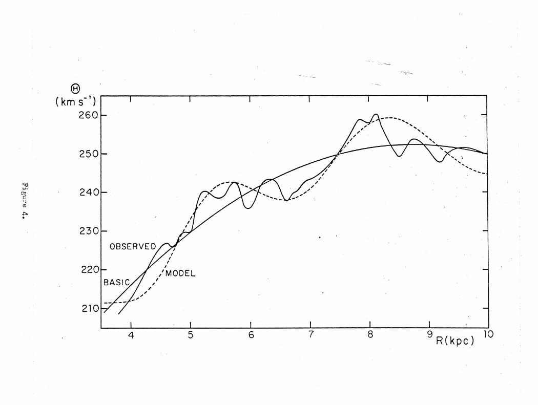
0(km s')

260

!-i"CL

4 5 6 7 8R(kpc)

10

800

600

5C ~ 65

10 15DISTANCE FROM SUN (kpc) DISTANCE FROM SUN (kpc)

Figure 5.

2520

80- 1800

T(K)

40-

0

80

T(K)

40

0

80

T(K)

40

0

I I I 1 I 1I

. "-*.* **.

0 *00. .* "*

*"

*"

S( I I

l 1 I I1 1 I i Ii I I 1

.°*

00000

L= 9Oo .. * *. . -- " 0

0.0

, 0 01

• "

. .. . . " . - . *

.- o0°"-00.

.,, °Oo oe" 18

."---o--- --'-

..I I!, ! I I, _ _ _ _ _ _ _ _ _ _ _ _

' ' * :

1 = l o . . .

r "o

- * *0 * '*L =10 **: . *.

* . .0

* :

0 0-* 0 0

"'**.- .. * **-'*--.. ...

- - ,** -I " I I

-120 -100 -80 -60 -40 -20V(km s-')

0 +20 +40

-1 I 1 -r r -r r r r . 7 --. -. ,-

""

1 I I I

I

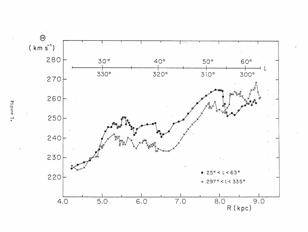
0(km s')

280

270

260

250

N"

300

3300

400 500

320 ° 3100

x

I

XX IX xxx

roc x-x'

* 25 ° < L < 630

x 297° <'L<335 0

[ __ !

6,0 7,0 8.0R (kpc)

r I ! f

600C

3000

240-

230

220

4.0 5,0. 9,0

1 -r -r - 1 . . - .. .

..

1_1 ,__. 1 - _ .. ! L

I-I

I ' I I I I ' I ' I ' I I I

- 150E-

Local

-H

- 100

E

- - 50H-

0

L

O 00LL_

0--

D

0+ 50

+ 150

+100

E

+ 50 >-I---

0-J

O0

LL0

5-0

- 50

- 100

2O 0 I.. . -150. .

- 200 r

i . -=

\' x

0.' **X, O: :*-*O -_ - "* **, - -

_..i ""\ "x "' i.=.=

-* ,*" ,<

xK x \ /x x

(x)-oxOx1xxxx x

- K- 18 < < 3600 . .. I0 < < 180

I I I I I t 1 1

0" x-x "

\x W . o . 01"00,-- ,""/-"" ""\\" i/.-"' , , .. -

-- x ( "\ (( X x )" "-x*~x"-

-- '- 1800 < < 360 °) x\xx_.x"-,,, ". x , %---- 0°< c < 180 °

+ 100

i 1 ,n ,

800 600 400 2001400 1200 1000

T~"

1800r

2000 220° 4° 20 2800 30 3200 340° 360°+2- -v

0-150

t v 10 1600

4110O

/""" -- \ 07 ' " " "- .. o\o"....

,\40

\\ 9

'**m.-.

70*

DENSITY-WAVE THEORY.

STREAMING MOTIONS\ \\

Vd~W.V0 6\

__60"

vs -9 \ \\o %\'

102

Iwoia 70

CENTER E - E / J $\| |

/ 4a 11 /,\' I ,'i\ it I , :

9 e " .- . -31/ 30 6 2-./I 70 7

Figure 9.

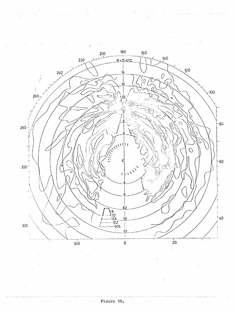
Figure 10.

0I ' I ' ' ' ' I ' ' '

(a) 1= 500 -4- 's -

1

r (kpc) -

8

12-

16-

i 1

(b)

INTENSITY(ARBITRARY SCALE) / I

I /

I \ /

1 20 -(c)

//

Tbc.(K) . , ,4-O - -\".

40 - *.*-''* :-

*. :,*

T b ( ) - , ,/.0•,0- \ 04 - **-*. ,* *. \ .-

0 --I , I I I I I I I

-60 -40 -20 0 +20 +40 +60 +80

V (km s-')-40 -20V (km s-')

T8 (K)9C

8C

7C

6C

5C

4C

3C

2CIC

C

(km s"1)

+ 20

0

- 20

- 40

- 60

- 80

-100

-120

(cm-3 )2.2

2.0

1.8

1.6

1.4

1.2

1.0

0.8

0.6

0.4

0.2

0.0

2 4 6r (kpc)

8 10 12

r (kpc)

' I ' I I I I

(a)

(b)

(c)

1 90°

/ "r',,i

r (kpc)

H

I i I I I I 1 I I l

1

1

1 I

1 I

1 I

V ,.: ,..i

.t

_ ~90'SUN --------

S :s -:Q

2.. \ ""80o"

70*

STREAMING MOTIONSVp - V o

6

8 0 60'

101o 1 ..,I2'

CENTERi

\ \50*

Fi s re 1 .

-100 -50 0 +50 +100 V(km/sec)

-100 -50 0 +50 +100

Fig re ! 4 .

100

90

80.

70.

60

50e

4so 0

30"

20

10

n

100

90O

80

70

60

50

40e

30

20

10

V(km/sec)

-100 -50 0 +50 +100 V(km/sec)

Model II

Circular rotation

100100

9 0O

800

7oe

60

50

30

2o"

10

-100 -50 0 +50 +100 V(km/sec)

Figure 15.

11

90

80

so"

7Co

60

50o

400

30e

2o

10

0 +50 V(km/s) +100r- -j , - T-- T - r-- - -- -- - - -T---- r-l

0 +50 V(krn/s) +100

Nw-

center r(kpc) 12

Figure 16.

90

80

70°

60*

50

10

.90°

80

70

60

50

40*

i

HIGMZ 7EXTENSION. 140' OW4i. LONGITUDE=35. LATITUDE--20 TO -20.

+20 0v

+18 6.D)11( 0 o

On 00,c

o f

+ 1

00

*6 *

-8 - .0

.+4 0 0

-012 -.

4- 0 0 ()V - -

- 2

* .

. cOI " 1\v

-6

-18 J1 o_ ,.

./ -i I - J .-2<

-16

I . , , I . i .LI,,1 ,, I .! , i , L , _ . . I

-160 -120 -80 -40 0 .40 +80 .120 +160

VELOCITY km/s (i.s.r.)

xc1.

-400

'

-600\

\\

800-/

N

\ 1

\

I II

1-800

/1

I-8600

Figure 18.

2000 14 0°.7 1000

-- 2400

I

\

II\

I \

I I

-400

20°

3000 327°.7i 0°0

/28

LI I r - -k} \ /'CAi If

y 100 1 f 4 1

CD~~j X1 -)Wl bIjo ' ?

/ j , I$I 0 VN 1

0-

r- ,-mc c-' -IJ Yf k

-250 -20-12-10-05050'0

V kms