the level 2 - esa earth observation dataearth.esa.int/smos07/pres/200_pres.pdf · p. waldteufel,...
TRANSCRIPT
YHK-PHW SMOS 7th Workshop Frascati
The SMOS Level 2
Y. H. Kerr, P. Waldteufel, P. Richaume, F. Cabot, A. Mialon, J-P. Wigneron, P. Ferrazzoli, A. Mahmoodi (and Array), MJ
Escorihuela, K. Saleh, S. Delwart …
and the SMOS team

YHK-PHW SMOS 7th Workshop Frascati
• Role of Soil moisture in surface atmosphere interactions:
storage of water (surface and root zone), water uptake by vegetation (root zone), fluxes at the interface (evaporation), influence on run-off
• Implies relevance forWeather ForecastsClimatic studiesWater resources crop managementForecast of extreme events
• Climate change predictions and rain event forecasts requires SST and SM
Science Objectives for SMOS: Soil Moisture
Houser, 2000
YHK-PHW SMOS 7th Workshop Frascati
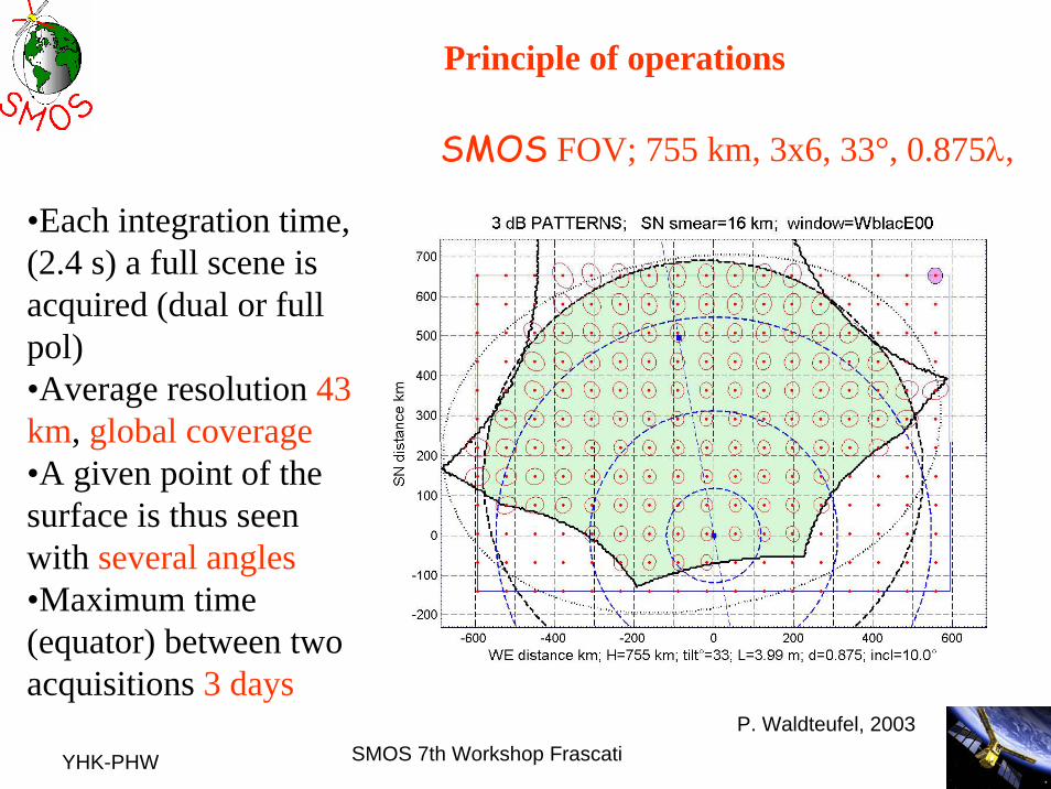
•Each integration time, (2.4 s) a full scene is acquired (dual or full pol)•Average resolution 43 km, global coverage•A given point of the surface is thus seen with several angles•Maximum time (equator) between two acquisitions 3 days
Principle of operations
SMOS FOV; 755 km, 3x6, 33°, 0.875λ,
P. Waldteufel, 2003

YHK-PHW SMOS 7th Workshop Frascati
The SMOSworld….And DGGs…
DFFG @ δkm
=300 km, for φ ∈ {−87,87} & λ ∈ {0,360}
Orthographic ProjectionP. Richaume 2006
YHK-PHW SMOS 7th Workshop Frascati
Level 2 algorithm rationale• To be ready at launch no statistical approaches at the
onset• Focussed on most common land surfaces with room for
extension has to work!• Physically based on validated models• Modular and upgradable as research progresses and
data is available / analysed• Relatively complex and to be simplified according to
actual measurements• Use of external data• We are bound to discover a few things• Described in ATBD +TGRD etc… most available• Small demo this evening

YHK-PHW SMOS 7th Workshop Frascati
Principle of SM retrievalFor each SMOS grid location, a vector of TBSMOS is provided for a list of incidence angles θm;Then the retrieval algorithm minimizes a cost function C:
( ) [ ] ( ) ∑ −+ΔΔ= −
ii
iim
tm
ppTBMCOVTBMC 2
201 ][
σ
where ..),..( imMODELSMOSm pTMTBTB θ−=Δ
pi are parameters of the model to be retrieved, with a priori values and standard deviations pi0 and σi. [COV] is the data covariance matrix

YHK-PHW SMOS 7th Workshop Frascati
Pre Processing filter SMOS views co-locate auxiliary data with DGG node compute aggregated mean cover fractions compute reference values
Iterative parameters retrievalfit the selected forward model to observations use other models for default contribution
Decision Tree select main fraction for retrieval select one model for retrieval select other models for default contributions
SMOS L1c Data products files Auxiliary files
SMOS L2 auxiliaryFixed reference Evolving reference User parameters file
TB models libraryforward models default models future models
Post Processing compute parameters posterior variances retrieval analysis and diagnostics compute modeled surface TB @ 42.5° generate flags
DGG node data iterator
Generate output data
User Data Productretrieved parameters parameters variances science & quality flags
Data Analysis Report
algorithms internal datafull flags
Do full retrieval again eliminate bad views decrease free number of parameters
Level 2:Soil moistureAlgorithm
layout
YHK-PHW SMOS 7th Workshop Frascati
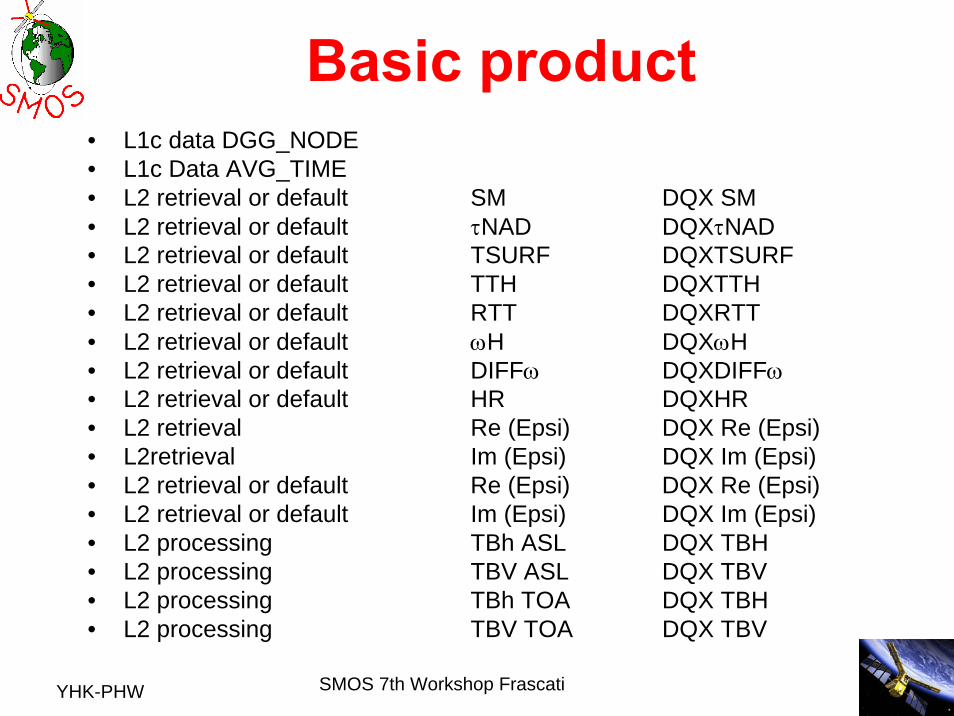
Basic product• L1c data DGG_NODE• L1c Data AVG_TIME• L2 retrieval or default SM DQX SM• L2 retrieval or default τNAD DQXτNAD• L2 retrieval or default TSURF DQXTSURF• L2 retrieval or default TTH DQXTTH• L2 retrieval or default RTT DQXRTT• L2 retrieval or default ωH DQXωH• L2 retrieval or default DIFFω DQXDIFFω• L2 retrieval or default HR DQXHR • L2 retrieval Re (Epsi) DQX Re (Epsi)• L2retrieval Im (Epsi) DQX Im (Epsi)• L2 retrieval or default Re (Epsi) DQX Re (Epsi)• L2 retrieval or default Im (Epsi) DQX Im (Epsi)• L2 processing TBh ASL DQX TBH• L2 processing TBV ASL DQX TBV• L2 processing TBh TOA DQX TBH• L2 processing TBV TOA DQX TBV

YHK-PHW SMOS 7th Workshop Frascati
Teodosio Lacava – IMAA-CNR
Projection: EASE Grid Global; Datum: WGS-84
0 5010 4020 30
Mean Soil Moisture (% volume): April 2003-2005 A
AMSR-E data
YHK-PHW SMOS 7th Workshop Frascati
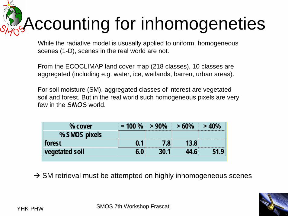
Accounting for inhomogenetiesWhile the radiative model is ususally applied to uniform, homogeneous scenes (1-D), scenes in the real world are not.
From the ECOCLIMAP land cover map (218 classes), 10 classes are aggregated (including e.g. water, ice, wetlands, barren, urban areas).
For soil moisture (SM), aggregated classes of interest are vegetated soil and forest. But in the real world such homogeneous pixels are very few in the SMOS world.
% cover = 100 % > 90% > 60% > 40% % SMOS pixels
forest 0.1 7.8 13.8 vegetated soil 6.0 30.1 44.6 51.9
SM retrieval must be attempted on highly inhomogeneous scenes
YHK-PHW SMOS 7th Workshop Frascati
Specific issues
• It is necessary to account for cover and surface inhomogeneities
• It is wished to make the best of SMOS data
This leads to
• Extensive use of auxiliary information
• Build several retrieval options organized according to a decision tree

YHK-PHW SMOS 7th Workshop Frascati
What is in a Pixel?!!!Working Area @ DGG ID #32002432 [φ = 44.42°, λ = −1.115°, 123 km x 123 km]
EEAP DFFG @ δkm
= 4 km, Zone #72
Albers Equal−Area 2oW 30’ 1oW 30’ 0o
40’
44oN
20’
40’
45oN
Working area contains all
the footprints and more
Nodes spatial sampling
Elementary surfaces (DFFG)
Richaume et al 2006
YHK-PHW SMOS 7th Workshop Frascati
Issues: What is inside a pixel?• Decision tree set of models
– Fixed features:• Low vegetation, forested, barren, water, permanent snow/ice,
urban– Variable features
• Snow, variable water bodies/ floods, frozen ground/ vegetation
– Overlapping perturbing factors• Topography, RFI
– Issues:• Knowledge• Temporal signatures

YHK-PHW SMOS 7th Workshop Frascati
Models and mixed pixels
global B T at S M O Santennas
S ynthetic antenna d irectional ga ind i
e1 e2 e3 e4 e5 e6 e7 e8 e9
G 2
G 5
type 1 em itter ⇒ C F 1
type 2 em itter ⇒ C F 2
type 3 em itter ⇒ C F 3
anten na footprin t
G 7
: Aggregated fractions FM0 and FM
FM0 class Aggregated land cover FM class Complementarity A B C D E
FNO Vegetated soil + sand FNO FFO Forest FFO FWL Wetlands FWL
Open fresh water FWP Open saline water FWS
FWO Open water FEB Barren FEB FTI Total Ice fraction
Ice & permanent snow FEI Sea Ice FSI
FUL Low urban coverage
FUM Moderate urban coverage
Comple-mentary
Sum of comple-mentary fractions equals unity
FTS Strong topography FTM Moderate topography FRZ Frost FRZ
Non permanent dry snow Non permanent wet snow FSN Non permanent mixed snow
FSN
Supple-mentary
Supple-mentary fractions are super-imposed
Set of models for each surface type

YHK-PHW SMOS 7th Workshop Frascati
Pure pixels?...
15oW 10oW 5oW 0o 5oE 10oE
42oN
45oN
48oN
51oN
54oN WA_DGG_exact
Colour code/ ● ocean, ● inland water body, ● rivers, ● All others, ● WA_DGG_nowater;
Richaume et al 2006
YHK-PHW SMOS 7th Workshop Frascati
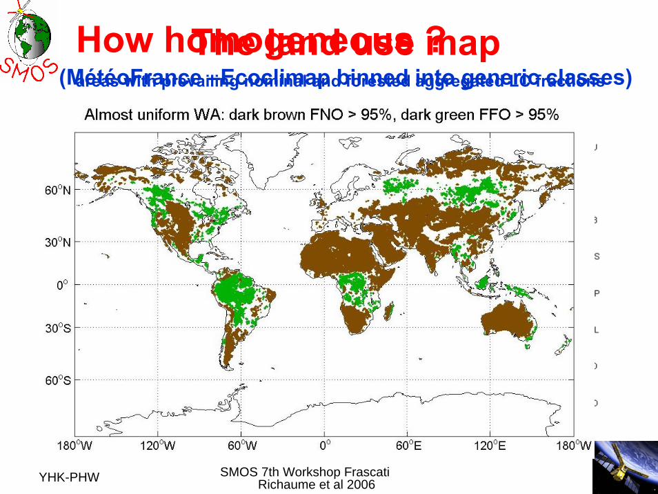
The land use map (MétéoFrance –Ecoclimap binned into generic classes)How homogeneous ?areas with prevailing nominal and forested aggregated LC fractions
Richaume et al 2006

YHK-PHW SMOS 7th Workshop Frascati
In conclusion: SM retrievals can be attempted in many areas with varying
expected accuracy
Richaume et al 2006

YHK-PHW SMOS 7th Workshop FrascatiRichaume et al 2007
YHK-PHW SMOS 7th Workshop Frascati
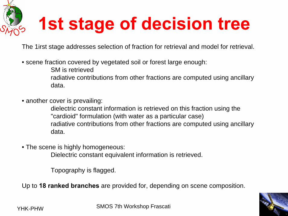
1st stage of decision treeThe 1irst stage addresses selection of fraction for retrieval and model for retrieval.
• scene fraction covered by vegetated soil or forest large enough:SM is retrievedradiative contributions from other fractions are computed using ancillarydata.
• another cover is prevailing:dielectric constant information is retrieved on this fraction using the "cardioid" formulation (with water as a particular case)radiative contributions from other fractions are computed using ancillarydata.
• The scene is highly homogeneous:Dielectric constant equivalent information is retrieved.
Topography is flagged.
Up to 18 ranked branches are provided for, depending on scene composition.
YHK-PHW SMOS 7th Workshop Frascati
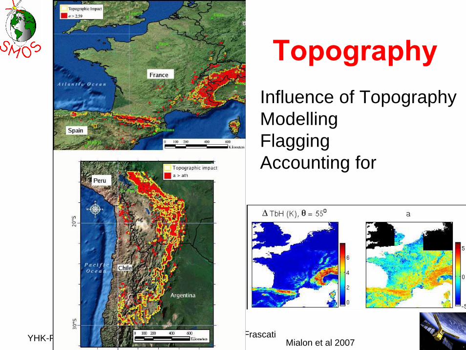
TopographyInfluence of TopographyModellingFlaggingAccounting for
Mialon et al 2007

YHK-PHW SMOS 7th Workshop Frascati
2nd stage of decision treeThe second stage of decision tree addresses the selection of additional parameters to be retrieved, and associated a priori constraints (while initial values are obtained from auxiliary information).
Retrieval potential for SM depends mainly on:• Incidence angle coverage ; decreases as swath abscissa increases away from track and spurious data are removed• Equivalent vegetation nadir optical thickness τ
9 branches are defined (3 for θ coverage, 3 for τ initial value)SM and τ are always retrieved. Selected additional parameters are • vegetation albedo and coefficient for variation of optical thickness with θ.• Coefficient in soil roughness modelling (although the retrieval potential is weak).

YHK-PHW SMOS 7th Workshop FrascatiWaldteufel et al., 2007
YHK-PHW SMOS 7th Workshop Frascati
Algorithm validation• Before launch
– Test pattern– Synthetic « realistic » orbit– Assembled ground data
• After launch– Cal Val exercises– Cofrontation with other measurements
Initiated (2005)– GEWEX soil moisture network
YHK-PHW SMOS 7th Workshop Frascati
Algorithm validation PlanDirect simulation Lo-
op Selection x / + N data set
Data options for DQX runs 792 TBL1Surface scene
Scene homogeneous nominal ; suggested code 166WEF none necessary
Input parameters for simulated dataSM SL 0.0 to 0.5 step 0.1 x 6TAU TL1 0, 0.01, 0.025, 0.05, 0.1, 0.2, 0.3, 0.4, 0.5, 0.6, 0.7, 0.8 x 12Sand, clay 0.4, 0.3Tsurf 288Tsky 3.7T0 atm, P0, WVC 288, 1013, 3ro_s, alpha, SAL, eps_pa From UPF LUTHR, NR_H, etc. from CLASS LUT for selected code
Input observation conditionsRadiometric uncertainty simulated based on L1c test scenarioX_SWATH (km) XL 0, 100, 200, 300, 350, 400, 425, 450, 475, 500, 525 x 11Incidence & rotation angles from L1c test scenarioFaraday angles from L1c test scenarioL1c flags from L1c test scenario
Additional data options for bias runs 726Radiometric uncertainty Zeronon uniform TAU Mixing 2 direct models with TAU=0 and 0.6 + 1 TBL3
non uniform SM TL2 Mixing 2 direct models with 2 SM TBD around loop value, for TAU=0 to 0.6 step 0.2 + 4 TBL4
Faraday angle TL2 Double L1_TS values; TAU=0 to 0.6 step 0.2 + 2 TBL5Rotation angle TL2 2° uniform; TAU=0 to 0.6 step 0.2 + 4 TBL6SM SL 0.0 to 0.5 step 0.1 x 6X_SWATH XL 0, 100, 200, 300, 350, 400, 425, 450, 475, 500, 525 x 11
Total 1518
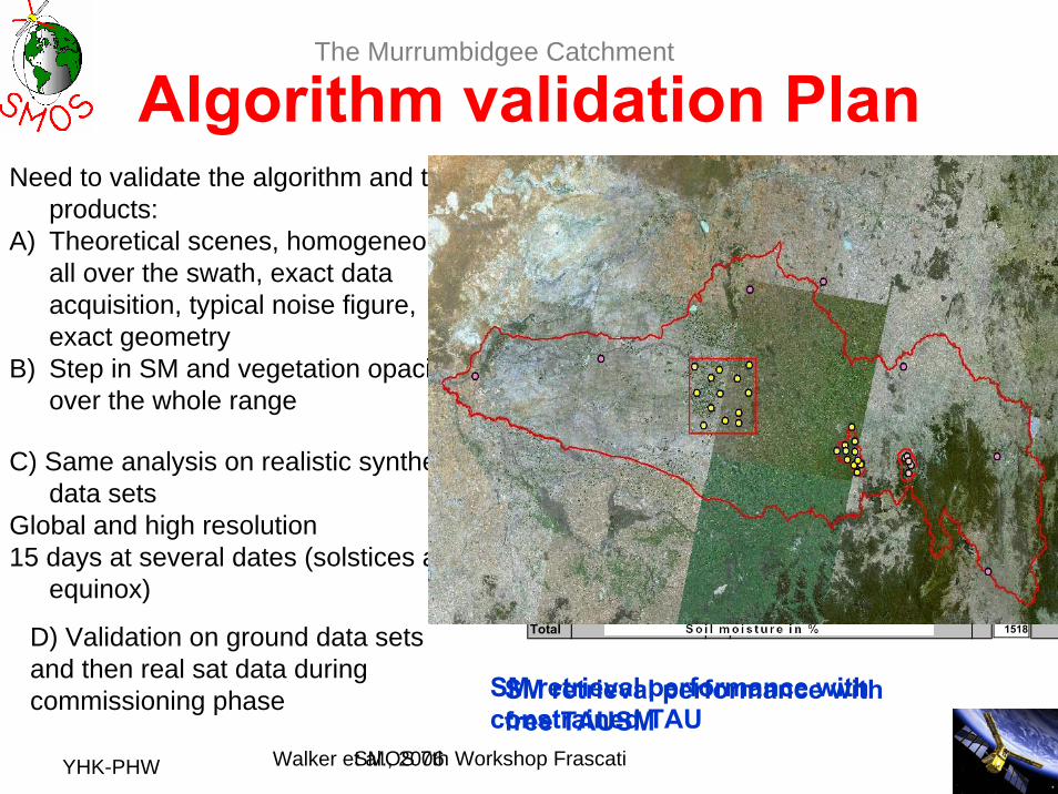
Need to validate the algorithm and the products:
A) Theoretical scenes, homogeneous, all over the swath, exact data acquisition, typical noise figure, exact geometry
B) Step in SM and vegetation opacity over the whole range
C) Same analysis on realistic synthetic data sets
Global and high resolution15 days at several dates (solstices and
equinox)
D) Validation on ground data sets
The Murrumbidgee Catchment
and then real sat data during commissioning phase SM retrieval performance with
free TAUSMSM retrieval performance with constrained TAU
Walker et al., 2006
YHK-PHW SMOS 7th Workshop Frascati
Issues• Dielectric constant models
– Near 0– For dry bare soils
• Litter effect• Surface roughness• Water bodies
• Varying features (Frozen, snow)• Perturbations (rain interception)• RFI• Unknown surfaces (urban, barren ….)• And things to discover….

YHK-PHW SMOS 7th Workshop Frascati
Steps: a recap• Homogeneous areas• Two to 4 cover types• Testing decision tree branches• Realistics scenes• Real scenes• And bugs/ issues to discover….

YHK-PHW SMOS 7th Workshop Frascati
Test pattern
Mialon et al 2007

YHK-PHW SMOS 7th Workshop Frascati
Algorithm outputWaldteufel et al., 2006
YHK-PHW SMOS 7th Workshop Frascati
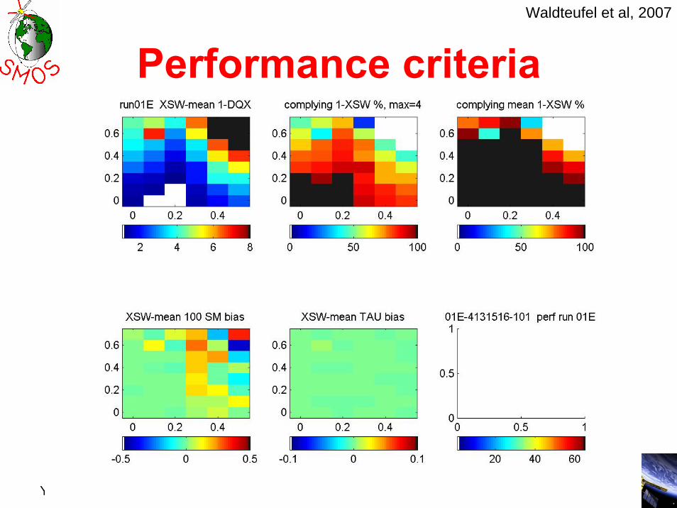
Performance criteriaWaldteufel et al, 2007
YHK-PHW SMOS 7th Workshop Frascati
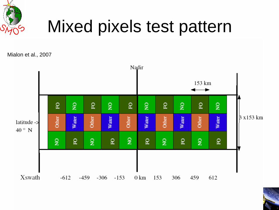
Mixed pixels test patternMialon et al., 2007
YHK-PHW SMOS 7th Workshop Frascati
Some results (CESBIO+Array)
• Latest out put from the L2 SMPPD– Surface high resolution data (ecoclimap) (1 4 km)– ISBA model outputs for forcings converted to ECMWF
grib– SEPSBIO simulations
• SEPS + GS + LMEB -> Algo BB
– L1c production– Inverse algorithm
• Africa• Europe

YHK-PHW SMOS 7th Workshop Frascati
The area

YHK-PHW SMOS 7th Workshop Frascati
Isba
Cabot et al., 2007

YHK-PHW SMOS 7th Workshop Frascati
Snapshots
Cabot et al., 2007

YHK-PHW SMOS 7th Workshop Frascati
Browse
Cabot et al., 2007
YHK-PHW SMOS 7th Workshop Frascati
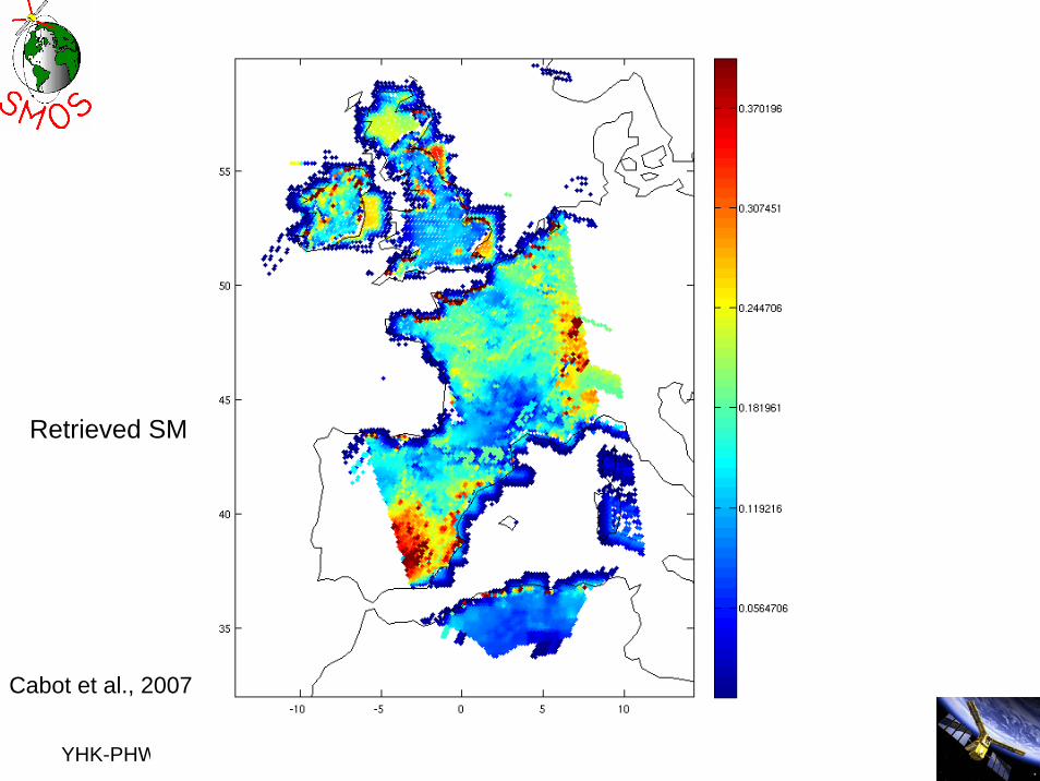
Retrieved SM
Cabot et al., 2007
YHK-PHW SMOS 7th Workshop Frascati
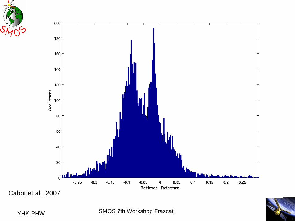
Cabot et al., 2007

YHK-PHW SMOS 7th Workshop Frascati
ISBA
Cabot et al., 2007

YHK-PHW SMOS 7th Workshop Frascati
Snapshots
Cabot et al., 2007

YHK-PHW SMOS 7th Workshop Frascati
Browse
Cabot et al., 2007
YHK-PHW SMOS 7th Workshop Frascati
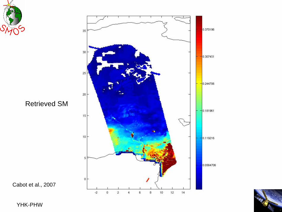
Retrieved SM
Cabot et al., 2007

YHK-PHW SMOS 7th Workshop FrascatiNB 87’ forcings and ’88’ initCabot et al., 2007
YHK-PHW SMOS 7th Workshop Frascati
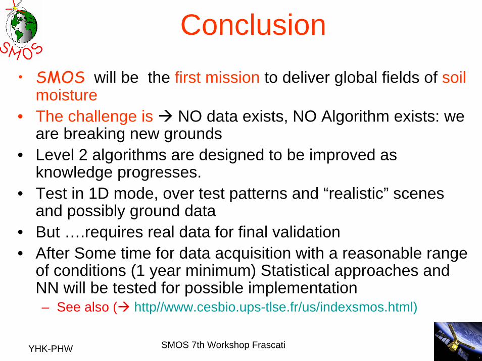
Conclusion• SMOS will be the first mission to deliver global fields of soil
moisture• The challenge is NO data exists, NO Algorithm exists: we
are breaking new grounds • Level 2 algorithms are designed to be improved as
knowledge progresses.• Test in 1D mode, over test patterns and “realistic” scenes
and possibly ground data• But ….requires real data for final validation• After Some time for data acquisition with a reasonable range
of conditions (1 year minimum) Statistical approaches and NN will be tested for possible implementation – See also ( http//www.cesbio.ups-tlse.fr/us/indexsmos.html)
YHK-PHW SMOS 7th Workshop Frascati
Thank you …..Any questions ? http//www.cesbio.ups-tlse.fr/us/indexsmos.html