the libor market model: from theory to calibration · sommario questa tesi `e incentrata su un...
TRANSCRIPT

Alma Mater Studiorum · Universita di
Bologna
FACOLTA DI SCIENZE MATEMATICHE, FISICHE E NATURALI
Corso di Laurea Magistrale in Matematica
- Curriculum Applicativo -
The Libor Market Model:
from theory to calibration
Tesi di Laurea in Equazioni Differenziali Stocastiche
in Finanza Matematica
Relatore:
Chiar.mo Prof.
Andrea Pascucci
Presentata da:
Candia Riga
I Sessione di Laurea: 24 Giugno 2011
Anno Accademico 2010/2011


Acknowledgements
I am heartily thankful to my supervisor, Andrea Pascucci, who gave
me the right directions for studying the subject and, above all, guided me
throughout my studies and my dissertation. Then, it is a pleasure to thank
the others who have played an important role by accompanying me in the
studies that are object of my thesis, in particular Paolo Foschi and Giacomo
Ricco. Thanks also to Unipol UGF Banca e Assicurazioni.
Furthermore, I would like to thank my university colleagues and my
friends, who shared with me these two years, and my partner, who has always
supported me. Last but not least, I will be forever grateful to my family,
that made all this possible.


Abstract
This thesis is focused on the financial model for interest rates called the
LIBOR Market Model, which belongs to the family of market models and
it has as main objects the forward LIBOR rates. We will see it from its
theoretical approach to its calibration to data provided by the market. In
the appendixes, we provide the theoretical tools needed to understand the
mathematical manipulations of the model, largely deriving from the theory of
stochastic differential equations. In the inner chapters, firstly, we define the
main interest rates and financial instruments concerning with the interest rate
models. Then, we set the LIBOR market model, demonstrate its existence,
derive the dynamics of forward LIBOR rates and justify the pricing of caps
according to the Black’s formula. Then, we also present the model acting as
a counterpart to the LIBOR market model, that is the Swap Market Model,
which models the forward swap rates instead of the LIBOR ones. Again,
even this model is justified by a theoretical demonstration and the resulting
formula to price the swaptions coincides with the one used by traders in the
market, i.e. the Black’s formula for swaptions. However, the two models are
not compatible from a theoretical point, because the dynamics that would
be obtained for the swap rate, by starting from the dynamics of the LIBOR
market model, is not log-normal as instead is in the swap market model.
Took note of this inconsistency, we select the LIBOR market model and
derive various analytical approximating formulae to price the swaptions. It
will also be explained how to perform a Monte Carlo algorithm to calculate
the expectation of any payoff involving such rates by a simulation. Finally, it
will be presented the calibration of the LIBOR market model to the markets
of both caps and swaptions, together with various examples of application to
the historical correlation matrix and the cascade calibration of the forward
volatilities to the matrix of implied swaption volatilities provided by the
market.


Sommario
Questa tesi e incentrata su un modello di mercato per i tassi d’intersse detto
LIBOR Market Model, il quale modellizza i tassi forward LIBOR, a par-
tire dalla sua impostazione teorica fino alla sua calibrazione ai dati forniti
dal mercato. Nelle appendici vengono forniti gli strumenti teorici necessari
per la gestione matematica del modello, derivanti in gran parte dalla teo-
ria delle equazioni differenziali stocastiche. Nei capitoli interni, innanzitutto
vengono definiti i principali tassi di interesse e gli strumenti finanziari alla
base dei modelli di mercato sui tassi d’interesse. Poi viene impostato il LI-
BOR market model, dimostrata la sua esistenza, ricavate le dinamiche dei
tassi forward LIBOR e i prezzi dei cap, fedeli alla formula di Black. Viene
poi presentato anche il modello che funge da controparte al LIBOR market
model, ovvero lo Swap Market Model, che modellizza i tassi forward swap
anziche i LIBOR. Anche in questo modello si giustifica, mediante una dimo-
strazione teorica, una formula usata dai traders sul mercato per prezzare le
swaption, ovvero la formula di Black per le swaption. Tuttavia, i due modelli
non sono compatibili dal punto di vista teorico, in quanto la dinamica che
si otterrebbe per il tasso swap a partire dalle dinamiche del LIBOR market
model non e log-normale come invece e nello swap market model. Preso at-
to di questa inconsistenza, viene scelto il LIBOR market model e vengono
derivate diverse formule analitiche approssimate per prezzare le swaption.
Inoltre e spiegato come realizzare l’algoritmo di Monte Carlo per calcolare
tali prezzi mediante una simulazione. Infine viene presentata la calibrazione
del suddetto modello al mercato dei cap e a quello delle swaption, con diversi
esempi di applicazione alla calibrazione della matrice di correlazione storica e
alla calibrazione a cascata delle volatilita forward alla matrice delle volatilita
implicite di mercato delle swaption.


Abbreviations and Notations
w.r.t. = with respect to
s.p. = stochastic process
s.t. = such that
a.s. = almost surely
SDE = stochastic differential equation
B.m. = Brownian motion
EMM = equivalent martingale measure
e.g. = exempli gratia ≡ example given
i.e. = id est ≡ that is
IRS = Interest Rate Swap
PFS = Payer Interest Rate Swap
RFS = Receiver Interest Rate Swap
PFS = Payer Interest Rate Swap
LMM = LIBOR Market Model
SMM = Swap Market Model
c.d.f. = cumulative distribution function
iii

iv
r.v. = random variable(s)
E = expectation
Std = standard deviation
i.i.d. = independent identically distributed

Contents
Abbreviations and Notations iv
Introduction 7
1 Interest rates and basic instruments 11
1.1 Forward Rates . . . . . . . . . . . . . . . . . . . . . . . . . . . 16
Interest Rate Swaps . . . . . . . . . . . . . . . . . . . . . . . . 19
1.2 Main derivatives . . . . . . . . . . . . . . . . . . . . . . . . . . 22
Interest rate Caps/Floors . . . . . . . . . . . . . . . . . . . . . 22
Swaptions . . . . . . . . . . . . . . . . . . . . . . . . . . . . . 23
2 The LIBOR Market Model (LMM) 25
2.1 Pricing Caps in the LMM . . . . . . . . . . . . . . . . . . . . 31
3 The Swap Market Model (SMM) 34
3.1 Pricing Swaptions in the SMM . . . . . . . . . . . . . . . . . . 36
3.2 Theoretical incompatibility between LMM and SMM . . . . . 37
4 Pricing of Swaptions in the LMM 39
4.1 Monte Carlo Pricing of Swaptions . . . . . . . . . . . . . . . . 39
4.2 Approximated Analytical Swaption Prices . . . . . . . . . . . 46
4.2.1 Rank-One analytical Swaption prices . . . . . . . . . . 46
4.2.2 Rank-r analytical Swaption prices . . . . . . . . . . . . 53
4.2.3 Rebonato’s approximation . . . . . . . . . . . . . . . . 55
4.2.4 Hull and White’s approximation . . . . . . . . . . . . . 58
1

2 CONTENTS
4.3 Example: computational results of the different methods of
swaption pricing . . . . . . . . . . . . . . . . . . . . . . . . . . 59
5 Instantaneous Correlation Modeling 62
5.1 Full-rank parameterizations . . . . . . . . . . . . . . . . . . . 64
5.1.1 Low-parametric structures by Schoenmakers and Coffey 69
5.1.2 Classical two-parameter structure . . . . . . . . . . . . 73
5.1.3 Rebonato’s three-parameter structure . . . . . . . . . . 73
5.2 Reduced rank parameterizations . . . . . . . . . . . . . . . . . 74
5.2.1 Rebonato’s angles method . . . . . . . . . . . . . . . . 75
5.2.2 Reduced rank approximations of exogenous correlation
matrices . . . . . . . . . . . . . . . . . . . . . . . . . . 75
6 Calibration of the LMM 78
6.1 Calibration of the LMM to Caplets . . . . . . . . . . . . . . . 78
6.1.1 Parameterizations of Volatility of Forward Rates . . . . 78
6.1.2 The Term Structure of Volatility . . . . . . . . . . . . 84
7 Calibration of the LMM to Swaptions 91
7.1 Historical instantaneous correlation . . . . . . . . . . . . . . . 93
7.1.1 Historical estimation . . . . . . . . . . . . . . . . . . . 93
7.2 Cascade Calibration . . . . . . . . . . . . . . . . . . . . . . . 105
7.2.1 Triangular Cascade Calibration Algorithm . . . . . . . 106
7.2.2 Rectangular Cascade Calibration Algorithm . . . . . . 110
7.2.3 Extended Triangular Cascade Calibration Algorithm . 113
A Preliminary theory 121
B Change of measure 125
C Change of Measure with Correlation in Arbitrage Theory 130
D Change of numeraire 135
Forward measure . . . . . . . . . . . . . . . . . . . . . . . . . . . . 138

CONTENTS 3
Bibliography 141

List of Figures
4.1 Zero-bond curve obtained from market data in April 26,2011. . 60
6.1 Term structure of volatility Tj 7→ vTj+1−capl from the Euro
market, on May 4, 2011; the resettlement dates T0, . . . , TM
are annualized and expressed in years. . . . . . . . . . . . . . 85
6.2 Evolution of the term structure of volatility of Figure 6.1.2
obtained by calibrating the parametrization (6.5). . . . . . . . 87
6.3 Evolution of the term structure of volatility of Figure 6.1.2
obtained with parametrization (6.7). . . . . . . . . . . . . . . 89
7.1 Implied volatilities obtained by inverting the Black’s formula
for swaption, with swaption prices from the Euro market, May
4, 2011. . . . . . . . . . . . . . . . . . . . . . . . . . . . . . . 92
7.2 Three-dimensional plot of correlations ρi,j from the estimated
matrix in Figure 7.3. . . . . . . . . . . . . . . . . . . . . . . . 95
7.3 Estimated correlation matrix ρ obtained by historical data
from the Euro market, March 29, 2011. . . . . . . . . . . . . . 97
7.4 Three-dimensional plot of correlations ρRebi,j (α, β, ρinf) with the
values above for the parameters. . . . . . . . . . . . . . . . . . 98
7.5 Rebonato’s three-parameter structure approximating the his-
torically estimation ρ found in Figure 7.3. . . . . . . . . . . . 99
7.6 Three-dimensional plot of correlations ρSCi,j . . . . . . . . . . . . 101
4

LIST OF FIGURES 5
7.7 Schoenmakers and Coffey’s semi-parametric correlation struc-
ture estimated by historical data from the Euro market, March
29, 2011. . . . . . . . . . . . . . . . . . . . . . . . . . . . . . . 102
7.8 Three-dimensional plot of correlations ρSCpari,j . . . . . . . . . . . 103
7.9 Schoenmakers and Coffey’s three-parameter structure approx-
imating the historically estimation ρ found in Figure 7.3. . . . 104
7.10 Implied Black swaption volatilities, from the Euro market,
April 26, 2011. . . . . . . . . . . . . . . . . . . . . . . . . . . 111
7.11 Forward volatilities calibrated to the 5 × 5 sub-matrix of the
swaption table in Figure 7.10. . . . . . . . . . . . . . . . . . . 111
7.12 Forward volatilities calibrated to the 5 × 5 sub-matrix of the
swaption table in Figure 7.10. . . . . . . . . . . . . . . . . . . 114
7.13 Forward volatilities calibrated with a 10-dimensional ExtCCA
to the swaption table in Figure 7.10. . . . . . . . . . . . . . . 117
7.14 Black swaption volatilities partially reconstructed after a 10-
dimensional ExtCCA to the market swaption table in Fig-
ure 7.10. . . . . . . . . . . . . . . . . . . . . . . . . . . . . . . 118
7.15 Forward volatilities calibrated with a 15-dimensional ExtCCA
to the swaption table in Figure 7.10. . . . . . . . . . . . . . . 119
7.16 Black swaption volatilities partially reconstructed after a 15-
dimensional ExtCCA to the market swaption table in Fig-
ure 7.10. . . . . . . . . . . . . . . . . . . . . . . . . . . . . . . 120

List of Tables
4.1 Approximated prices of three payer swaptions with different
maturities and tenors, respectively by Rebonato’s, Hull and
White’s, Brace’s rank-1 and Brace’s rank-3 formulae and Monte
Carlo simulation with 100000 scenarios and a time grid of step
dt = 1360
y. . . . . . . . . . . . . . . . . . . . . . . . . . . . . . 61
6.1 General Piecewise-Constant volatilities. . . . . . . . . . . . . . 79
6.2 Time-to-maturity-dependent volatilities. . . . . . . . . . . . . 80
6.3 Constant maturity-dependent volatilities. . . . . . . . . . . . . 81
6.4 ΦiΨβ(t) structure . . . . . . . . . . . . . . . . . . . . . . . . . 82
6.5 ΦiΨi−(β(t)−1) structure . . . . . . . . . . . . . . . . . . . . . . 83
7.1 Average relative errors, both simple and squared, between his-
torical estimation in Figures 7.3-7.2 and, respectively, the ones
in Figures 7.5-7.4, 7.7-7.6 and 7.9-7.8. . . . . . . . . . . . . . . 105
7.2 Table summarizing the swaption volatilities to which we cali-
brate the LMM through a triangular cascade calibration and
the dependence of the GPC forward volatilities on them, where
the blue ones are the new parameters determined at each step. 107
7.3 Table summarizing the swaption volatilities to which we cali-
brate the LMM through a rectangular cascade calibration and
the dependence of the GPC forward volatilities on them, where
the blue ones are the new parameters determined at each step. 112
6

Introduction
In this thesis we present the most promising family of interest rate models,
that are the market models. The two main representatives of this family are
the LIBOR Market Model (LMM), which models the forward LIBOR rates
as the primary objects in an arbitrage free way instead of deriving it from the
term structure of instantaneous rates, and the Swap Market Model (SMM),
which models the dynamics of the forward swap rates. The advantages of
them is that, by choosing a deterministic volatility structure for the dynamics
of the rates modeled, the first one prices caps according to the Black’s cap
formula, whereas the second one prices swaptions according to the Black’s
swaption formula. Indeed, these Black’s formulae are the standard ones
used respectively in the cap and swaption markets, which are the two main
markets in the interest-rate derivatives world. Despite the good premises, the
desirable compatibility between the two market formulae is not theoretically
confirmed.
The LIBOR Market Model came out at the end of the 90s, in particular
it was rigorously introduced in 1997 by Brace, Gatarek and Musiela, ”The
Market Model of Interest Rate Dynamics”, then other significant contributes
came by Jamshidian, ”LIBOR and swap market models and measures”, and
Miltersen, Sandmann and Sondermann, ”Closed Form Solutions for Term
Structure Derivates with Log-Normal Interest Rates”, all in 1997. At the
same time, Jamshidian introduced the Swap Market Model, in 1997.
The point of this work is to analyze in detail the LIBOR market model,
from its theoretical setting and mathematical results to its financial and prac-
7

8 LIST OF TABLES
tical use, together with some practical applications referring to the current
market data. This thesis is structured as follows.
Appendixes. We give a synthetic presentation of the mathematical defi-
nitions and the main theoretical results concerning the theory of the
stochastic processes and the stochastic differential equations. More-
over, we show the details of one of the most important tool in the
mathematical studying of financial markets, that is the change of nu-
meraire.
Chapter 1. We define the different types of interest rates and introduce
the basic financial instruments and the main derivatives we are dealing
with, i.e. caps and swaptions, together with their practically used
Black’s formulae.
Chapter 2. We introduce the LMM, derive the dynamics of the forward
LIBOR rate modeled and prove its existence. Then we introduce the
Black volatilities implied by the cap market and show that the risk-
neutral valuation formula of caps gives the same prices as the Black’s
cap formula.
Chapter 3. We introduce the SMM, prove that the pricing formula for
swaptions coincides with the Black’s swaption formula and show the
inconsistency of the dynamics assumed by the SMM with the ones
given by the LMM.
Chapter 4. We show in detail the different approaches to price swaptions
under the framework of the LMM, from the Monte Carlo simulation to
various analytical approximating formulae.
Chapter 5. We introduce the important and rich subject of the instanta-
neous correlation modeling, dealing with the modeling and parametriza-
tion of the correlations between the Brownian motions driving the dy-
namics of forward LIBOR rates.

LIST OF TABLES 9
Chapter 6. We introduce the calibration of the LMM to the cap market and
we present various plausible parameterizations for the forward volatility
structure. Then we consider, for each of them, the evolution in time of
the term structure of volatility.
Chapter 7. We introduce the calibration of the LMM to the swaption mar-
ket, in particular we show an exact cascade calibration. Moreover,
we introduce the use of a historical correlation matrix, along with its
computation and parametric calibration.


Chapter 1
Interest rates and basic
instruments
Definition 1.1. A zero-coupon bond (also known as pure discount bond)
with maturity date T , briefly called T -bond, is a contract which guarantees
the holder to be paid 1 unit of currency at time T , with no intermediate
payments. The contract value at time t < T is denoted by p(t, T ) .
We must make some assumptions:
- there exist a (frictionless) market for T -bond for every T > 0;
- p(T, T ) = 1 holds for all T > 0 (it avoids arbitrage);
- for all fixed t < T the application T 7→ p(t, T ) is differentiable w.r.t.
maturity time.
The graph of the function T 7→ p(t, T ) , T > t , called zero-bond curve,
is decreasing starting from p(t, t) = 1 and will be typically very smooth.
Whereas, for each fixed maturity T , p(t, T ) is a scalar stochastic process
whose trajectory will be typically very irregular (determined by a Brownian
motion).
The amount of time from the present date t and the maturity date T ,
called the time to maturity, is calculated in different ways, according to the
11

12 1. Interest rates and basic instruments
market convention (day-count convention). Once this last is made clear, the
measure of time to maturity, denoted by τ(t,T), is referred to as the year-
fraction between the dates t and T and it’s usually expressed in years. The
most frequently used day-count convention are:
- Actual/365 −→ a year is 365 days long and the year-fraction between
two dates is the actual number of days between them divided by 365;
- Actual/360 −→ a year is 360 days long and the year-fraction between
two dates is the actual number of days between them divided by 360;
- 30/360 −→ months are 30 days long, a year is 360 days long and the
year-fraction between two dates (d1, m1, y1) and (d2, m2, y2) is given by
the ratio
max(30− d1, 0) + min(d2, 30) + 360 · (y2 − y1) + 30 · (m2 −m1 − 1)
360.
In all the conventions adjustments may be included to leave out holidays.
Zero-coupon bonds are fundamental objects in the interest rate theory,
in fact all interest rates can be also defined in terms of zero-coupon bond
prices.
Talking about interest rates we need to distinguish the two main cate-
gories:
- government rates, related to bonds issued by governments;
- interbank rates, at which deposits are exchanged between banks and
swap transactions between them are.
We are considering the interbank sector of the market, however the mathe-
matical modeling of the resulting rates would be analogous in the two sectors.
Actually, interest rates are what is usually quoted in the (interbank)
financial markets, whereas zero-coupon bonds are theoretically instruments
not directly observable.

13
Definition 1.2. The continuously-compounded spot interest rate at time t
for the maturity T is the constant rate at which an investment of p(t, T ) unit
of currency at time t accrues continuously to yield 1 unit of currency at time
T .
It is denoted by R(t, T ) and is defined by:
R(t, T ) := − ln p(t, T )
τ(t, T ).
Equivalently:
eR(t,T )τ(t,T )p(t, T ) = 1 ,
from which we get the zero-coupon bond prices:
p(t, T ) = e−R(t,T )τ(t,T ) .
Definition 1.3. The simply-compounded spot interest rate at time t for the
maturity T is the constant rate at which an investment of p(t, T ) unit of
currency at time t accrues proportionally to the investment time to produce
1 unit of currency at time T .
It is denoted by L(t, T ) and is defined by:
L(t, T ) :=1− p(t, T )
τ(t, T )p(t, T ).
The most important interbank rate, as a reference for contracts, is the
LIBOR (London InterBank Offered Rate) rate, fixing daily at 12 o’ clock
in London. This is a simply-compounded spot interest rate, from which
derive the notation L for this last, and is typically linked to zero-coupon
bond prices by the ”Actual/360” day-count convention. Generally the term
”LIBOR” refers also to analogous rates fixing in other markets, e.g. the
EURIBOR rate (fixing in Bruxelles).
The bond prices in terms of LIBOR rate is:
p(t, T ) =1
1 + L(t, T )τ(t, T ).

14 1. Interest rates and basic instruments
Definition 1.4. The annually-compounded spot interest rate at time t for
the maturity T is the constant rate at which an investment of p(t, T ) unit
of currency at time t has to be reinvested once a year to produce 1 unit of
currency at time T .
It is denoted by Y (t, T ) and is defined by:
Y (t, T ) :=1
p(t, T )1
τ(t,T )
− 1 .
The day-count convention typically associated to the annual compound-
ing is the ”Actual/365”.
The bond prices in terms of these rates is:
p(t, T ) =1
(1 + Y (t, T ))τ(t,T ).
An extension of the annual compounding case is the following.
Definition 1.5. The k-times-per-year compounded spot interest rate at time
t for the maturity T is the constant rate at which an investment of p(t, T )
unit of currency at time t has to be reinvested k times a year to produce 1
unit of currency at time T .
It is denoted by Y k(t, T ) and is defined by:
Y k(t, T ) :=k
p(t, T )1
kτ(t,T )
− k .
All the above spot interest rates are equivalent in infinitesimal time in-
tervals. For this reason, we can define the short rate in the following way.
Definition 1.6. The instantaneous short interest rate at time t is the limit
of each of the different spot rates between times t and T with T → t+.
It is denoted by r(t) and is defined by:
r(t) = limT→t+
R(t, T )
= limT→t+
L(t, T )
= limT→t+
Y (t, T )
= limT→t+
Y k(t, T ) ∀k .

15
Based on this, we can define the mathematical representation of a bank
account, which accrues continuously according to the instantaneous rate.
Definition 1.7. The bank account (or money market account) at time t ≥ 0
is the value (the t-value) of a bank account with a unitary investment at
initial time 0.
It is denoted by B(t) and its dynamics is given by:
dB(t) = r(t)B(t)dt , B(0) = 1 ,
solved by:
B(t) = exp(
∫ t
0
r(s)ds) ,
as shown in (C.2). Notice that, according to the market setting (C.1)-
(C.2) and the theorem of change of drift with correlation, B is the only
asset in the market which is not modified when moving to a risk-adjusted
probability measure, in fact its instantaneous variation is not affected by a
change of measure.
The bank account is a stochastic process that provide us with a model of the
time value of money and allows us to build a discount factor of that value.
Definition 1.8. The (stochastic) discount factor between two time instants
t and T ≥ t is the amount of money at time t equivalent (according to the
dynamic of B(t)) at 1 unit of currency at time T .
It is denoted by D(t, T ) and is defined by:
D(t, T ) =B(t)
B(T )= exp
(−∫ T
t
r(s)ds
).
In some financial areas where the short rate r is considered a determin-
istic function of time (i.e. in markets where the variability of the rate is
negligible with respect to movements of the underlying assets of options to
be priced), both the bank account and the discount factor become determin-
istic processes and we have D(t, T ) = p(t, T ) for all (t, T ) . However, when
dealing with interest rate derivatives, the variability of primary importance

16 1. Interest rates and basic instruments
is just that of the rates themselves. In this case r is modeled as a stochastic
process and consequently D(t, T ) is a random value at time t which depends
on the future evolution of r up to T , whereas p(t, T ) is the t-value (known)
of a contract with maturity date T .
1.1 Forward Rates
Now we move to define the forward rates, that are characterized by three
time instants: the present time t, at which they are locked in, and two points
in future time, the expiry time T and the maturity time S, with t ≤ T ≤ S .
The forward rates can be defined in two different ways.
First approach to define forward rates
We start defining a contract at the current time t which allows us to make
an investment of 1 unit of currency at time T and to have a deterministic
rate of return (determined at t) over the period [T, S]. Then we compute the
relevant interest rate involved by solving an equation that avoids arbitrage.
The corresponding financial strategy is the following:
Time Operations Portfolio value
t sell one T -bond and use
the income p(t, T ) to buy p(t,T )p(t,S)
S-bonds 0
T pay out 1 −1
S receive the amount p(t,T )p(t,S)
−1 + p(t,T )p(t,S)
The net effect of all this, based on a contract made at time t, is that an
investment of 1 unit of currency at time T has yielded p(t,T )p(t,S)
at time S. Thus
it guarantees a riskless rate of interest over the future interval [T, S]. Such
an interest rate is what is called a forward rate and it can be characterized
depending on the compounding type, as follows.
Definition 1.9. The simply-compounded forward interest rate at time t for
the expiry T > t and maturity S > T is denoted by F (t;T, S) and is defined

1.1 Forward Rates 17
by:
F (t;T, S) :=1
τ(T, S)
(p(t, T )
p(t, S)− 1
). (1.1)
It is the solution to the equation
1 + τ(T, S)F =p(t, T )
p(t, S).
Definition 1.10. The continuously-compounded forward interest rate at time
t for the expiry T > t and maturity S > T is denoted by R(t;T, S) and is
defined by:
R(t;T, S) := − ln p(t, S)− ln p(t, T )
τ(T, S).
It is the solution to the equation
eRτ(T,S) =p(t, T )
p(t, S).
The simple rate notation is the one used in the market, whereas the contin-
uous one is used in theoretical contexts and does not regard the model we
are exposing.
Second approach to define forward rates
Definition 1.11. A forward rate agreement (FRA) is a contract stipulated
at the current time t that gives its holder an interest rate payment for the
period of time between the expiry T > t and the maturity S > T . Precisely,
at time S he receives a fixed payment based on a fixed rate K and pays a
floating amount based on the spot rate L(T, S) resetting in T .
Its S-payoff is thus:
Nτ(T, S)(K − L(T, S)) ,
where N is the contract nominal value.
This payoff can be rewritten by substituting the LIBOR rate with its
expression:
N
(τ(T, S)K − 1
p(T, S)+ 1
).

18 1. Interest rates and basic instruments
Now we use the principle of no arbitrage to calculate the value of the above
FRA at time t. The amount 1p(T,S)
at time S equals to have p(T, S) 1p(T,S)
= 1
unit of currency at time T , in turn this one equals to have p(t, T ) units of
currency at time t. Instead, the amount τ(T, S)K + 1 at time S equals to
have p(t, S)(τ(T, S)K+1) units of currency at time t. Therefore, the t-value
of the contract is
FRA(t, T, S, τ(T, S), N,K) = N [p(t, S)τ(T, S)K − p(t, T ) + p(t, S)]) .
(1.2)
Finally we can define the simply-compounded forward interest rate as the
unique value of the fixed rate K which renders the FRA with expiry T and
maturity S a fair contract at time t, i.e. such that the t-price (1.2) is 0, to
achieve the same Definition 1.9 again. Then, the value of the FRA can be
rewritten in terms of the forward rate as
FRA(t, T, S, τ(T, S), N,K) = N
[p(t, S)τ(T, S)K + p(t, S)
(1− p(t, T )
p(t, S)
)]
= N [p(t, S)τ(T, S)K+
+p(t, S)(−τ(T, S)F (t;T, S))]
= Nτ(T, S)p(t, S) (K − F (t;T, S)) . (1.3)
Comparing the payoff and the price of the above FRA, we can view the
forward rate F (t;T, S) as a kind of estimate of the future spot rate L(T, S),
which is random at time t.
The last type of interest rate worthy to be mentioned is the analogous of
the instantaneous short interest rate, in the future.
Definition 1.12. The instantaneous forward interest rate at time t for the
maturity T is the limit of the forward rates expiring in T when collapsing
towards their expiry.

1.1 Forward Rates 19
It is denoted by f(t) and is defined by:
f(t) = limS→T+
F (t;T, S)
= limS→T+
R(t;T, S)
= −∂ ln p(t, T )
∂T.
Interest Rate Swaps
Definition 1.13. Given the tenor structure T = Tα, . . . , Tβ with the corre-
sponding set of year fractions τ = τα, . . . , τβ, an Interest Rate Swap (IRS )
with tenor Tβ − Tα is a contract which, at every time Ti ∈ Tα+1, . . . , Tβexchanges the floating leg payment
NτiL(Ti−1, Ti)
with the fixed leg payment
NτiK ,
where N is the nominal value and K a fixed interest rate.
It can be of two types: the holder of a Payer IRS, denoted by PFS, re-
ceives the floating leg and pays the fixed leg, whereas the holder of a Receiver
IRS, denoted by RFS, the opposite. The discounted payoff at a time t < Tα
of a PFS is thus:
β∑
i=α+1
D(t, Ti)Nτi(L(Ti−1, Ti)−K) ,
whereas a RFS has the opposite payoff.

20 1. Interest rates and basic instruments
The arbitrage-free value at t < Tα of a PFS with a unit notional amount is:
PFS(t, T , K) = E
[β∑
i=α+1
D(t, Ti) τi (Fi(Ti−1)−K) | Ft
]
=
β∑
i=α+1
p(t, Ti) τi Ei [L(Ti−1, Ti)−K | Ft]
= p(t, Tα)− p(t, Tβ)−K
β∑
i=α+1
τi p(t, Ti) (1.4)
=
β∑
i=α+1
p(t, Ti) τi (Fi(t)−K) , (1.5)
where denoting Fj(t) := F (t;Tj−1, Tj) .
Proof. The formula (1.4) can be obtained analogously to the price of a FRA:
the floating payment set in Ti−1 and payed in Ti can be rewritten as
1
p(Ti−1, Ti)− 1 ,
that equals to have
p(t, Ti−1)− p(t, Ti) (1.6)
at time t < Tα, so that the arbitrage-free value at t of the whole floating side
isβ∑
i=α+1
(p(t, Ti−1)− p(t, Ti)) = p(t, Tα)− p(t, Tβ) ;
on the other hand the amount τiK at time Ti equals to have p(t, Ti)τiK units
of currency at time t, so that the arbitrage-free value at t of the whole fixed
side isβ∑
i=α+1
p(t, Ti)τiK = K
β∑
i=α+1
p(t, Ti)τi .
Equivalently we could have obtained (1.6) by the risk neutral pricing for-

1.1 Forward Rates 21
mula (D.6):
EQ
[D(t, Ti)
(1
p(Ti−1, Ti)− 1
)| FW
t
]=
= EQ
[e−
∫ Tit rsds
1
p(Ti−1, Ti)| FW
t
]− EQ
[D(t, Ti) | FW
t
]
= EQ
[e−
∫ Tit rsdsEQ
[e∫ TiTi−1
rsds | FWTi−1
]| FW
t
]− p(t, Ti)
= EQ[e−
∫ Ti−1t rsds | FW
t
]− p(t, Ti) = p(t, Ti−1)− p(t, Ti) .
Then, the formula (1.5) can be obtained by substituting the expression for
forward rates (1.1), as we made in (1.3).
From another point of view, a RFS can be view as a portfolio of FRAs,
valued through formulas (1.2) or (1.3), leading to a price opposite to that of
a PFS.
Definition 1.14. The forward swap rate (or par swap rate) of a Tα×(Tβ−Tα)
Interest Rate Swap is denoted by Sα,β(t) at time t and is defined as that value
of the fixed rate that makes the IRS a fair contract at the current time t. It
is obtained by equating to zero the t-value of the contract in (1.4):
Sα,β(t) :=p(t, Tα)− p(t, Tβ)
β∑i=α+1
τi p(t, Ti)
. (1.7)
Remark 1. It can be rewritten as a nonlinear function of the forward LIBOR
rates as
Sα,β(t) =
1−β∏
j=α+1
11+τjFj(t)
β∑i=α+1
τii∏
j=α+1
11+τjFj(t)
. (1.8)
Proof.
Sα,β(t) =p(t, Tα)− p(t, Tβ)
β∑i=α+1
τi p(t, Ti)
=
p(t,Tα)−p(t,Tβ)
p(t,Tα)
β∑i=α+1
τip(t,Ti)p(t,Tα)
,

22 1. Interest rates and basic instruments
then, from the definition (1.1) of forward rates and by a simple algebraic
relation, we have:
p(t, Ti)
p(t, Tα)=
i∏
j=α+1
p(t, Tj)
p(t, Tj−1)=
i∏
j=α+1
1
1 + τjFj(t)∀i > α .
1.2 Main derivatives
In this chapter we present the two main interest rate derivatives, that are
caps/floors and swaptions.
Interest rate Caps/Floors
Definition 1.15. An interest rate cap is a financial insurance contract equiv-
alent to a payer interest rate swap where each exchange payment is executed
if and only if it has positive value. The discounted payoff at time t of the cap
associated to the tenor structure T = Tα, . . . , Tβ, with the corresponding
set of year fractions τ = τα, . . . , τβ, and working on a principal amount of
money N , isβ∑
i=α+1
D(t, Ti)Nτi(L(Ti−1, Ti)−K)+ . (1.9)
Analogously, a floor is a contract equivalent to a receiver interest rate swap
where each exchange payment is executed if and only if it has positive value,
with t-discounted payoff
β∑
i=α+1
D(t, Ti)Nτi(K − L(Ti−1, Ti))+ .
A cap has the task of protecting the holder, indebted with a loan at a
floating rate of interest, from having to pay more than a prespecified rate K,
called the cap rate. On the other hand, a floor guarantees that the interest
paid on a floating rate loan will never be below a predetermined floor rate.

1.2 Main derivatives 23
A cap consists in a portfolio of a number of more basic contracts, named
caplets : the i-th caplet is determined at time Ti−1 but not paid out until
time Ti and has the t-discounted payoff
D(t, Ti)Nτi(L(Ti−1, Ti)−K)+ .
Analogously are defined the floorlet contracts.
The market practice is to price caps by using the Black’s formula for caps,
an extension of the Black and Scholes formula, dating back to 1976 when
Black had to price the payoff of commodity options. The price at time t of
the cap with tenor T and unit notional amount is
CapBlack(t, T , τ,K, v) =
β∑
i=α+1
τi p(t, Ti) Bl (K,F (t;Ti−1, Ti), vi)) , (1.10)
where
Bl(K,F (t;Ti−1, Ti), vi)) := F (t;Ti−1, Ti) Φ (d1(K,F (t;Ti−1, Ti), vi)) +
−KΦ (d2(K,F (t;Ti−1, Ti), vi)) ,
d1(K,F, u) :=ln( F
K )+u2
2
u,
d2(K,F, u) :=ln( F
K )−u2
2
u,
vi := v√Ti−1 ,
with the common volatility parameter v that is retrieved from market quotes.
Analogously, the Black’s formula for caplets is
CaplBlack(t, Ti−1, Ti, K, vi) = τi p(t, Ti) Bl (K,F (t;Ti−1, Ti), vi)) , (1.11)
for all i = α + 1, . . . , β.
Swaptions
Definition 1.16. A European Tα × (Tα − Tβ) Payer Swaption (PS ) with
swaption strike K is a contract that gives the right (but not the obligation)
to enter a PFS with tenor Tβ − Tα and fixed rate K at the future time Tα,
i.e. the swaption maturity.

24 1. Interest rates and basic instruments
Namely, a swaption is an option of an IRS. The payer swaption payoff at
its first reset date Tα, which is also the swaption maturity, is:
(PFS(Tα, T , K))+ =
(β∑
i=α+1
p(Tα, Ti) τi (F (Tα;Ti−1, Ti)−K)
)+
(1.12)
= (Sα,β(Tα)−K)+β∑
i=α+1
τi p(Tα, Ti) (1.13)
respectively in terms of forward rates and of the relevant forward swap rate.
Proof. The formula (1.12) is obtained simply by taking the positive part of
the Tα-price of a PFS in the form (1.5), whilst the formula (1.13) is obtained
from the other version (1.4) of the same price as follows:
(PFS(Tα, T , K))+ =
(p(Tα, Tα)− p(Tα, Tβ)−K
β∑
i=α+1
τi p(Tα, Ti)
)+
= (Sα,β(Tα)−K)+β∑
i=α+1
τi p(Tα, Ti) .
The market practice is to price swaptions by using the Black’s formula for
swaptions: the price at time t of the above Tα × (Tα − Tβ) payer swaption is
PSBlack(t, Tα, T , K, vα,β) =
β∑
i=α+1
τi p(t, Ti) Bl(K,Sα,β(t), vα,β
√Tα − t
).
(1.14)
A Receiver Swaption is defined analogously as an option on a RFS.

Chapter 2
The LIBOR Market Model
(LMM)
For a very long time, namely since the early ’80 to 1996, the market
practice has been to value caps, floors and swaptions by using a formal ex-
tension of the Black (1976) model. However, this formula was applied in a
completely heuristic way, under some simplifying and inexact assumptions.
Indeed, interest rate derivatives were priced by using short rate models, based
on modeling the instantaneous short interest rate; at one point this was as-
sumed to be deterministic, so that the discount factor was identified with the
corresponding bond price, that could be factorized out of the Q-expectation
in the risk-neutral pricing formula; then, inconsistently with the previous
assumption, the forward LIBOR rates were modeled as driftless geometric
Brownian motions under Q, hence stochastic; finally the expectation could be
view as the price of a call option in a market with zero risk-free rate, therefore
it was obtained through the Black’s formula. This is logically inconsistent.
Then, at the end of the ’90, after the coming of the theory of the change
of numeraire, a promising family of (arbitrage-free) interest rate models was
introduced: the Market Models. This breakthrough came at the hands of
Miltersen et al (1997), Brace et al (1997) and Jamshidian (1998). The prin-
cipal idea of these approaches is to choose a different numeraire than the
25

26 2. The LIBOR Market Model (LMM)
risk-free bank account.
The interest rate market is radically different from the others, e.g. commodi-
ties or equities, thus needs a own kind of modeling. There are three possible
choices in interest rate modeling: short rate models, that model one single
variable, instantaneous forward rate models, that model all infinite points of
the term structure and Market Models.
These recent ones have the following characteristics:
- instead of modeling instantaneous interest rates, they model a selection
of discrete real world rates (quoted in the market) spanning the term
structure;
- under a suitable change of numeraire these market rates can be modeled
log-normally;
- they produce pricing formulas for caps, floors and swaptions of the
Black-76 type;
- they are easy to calibrate to market data and are then used to price
more exotic products.
The model we are introducing is best known generally as ”LIBOR Mar-
ket Model” (LMM), or else ”Log-normal Forward LIBOR Model” or ”Brace-
Gatarek-Musiela 1997 Model” (BGM model), from the names of the authors
of the first published papers that rigorously described it.
Setting the model:
• t = 0 is the current time;
• the set T0, T1, . . . , TM of expiry-maturity dates (expressed in years) is
the tenor structure, with the corresponding year fractions τ0, τ1, . . . , τM,i.e. τi is the one associated with the expiry-maturity pair (Ti−1, Ti), for
all i > 0, and τ0 from now to T0;
• set T−1 := 0;

27
• the simply-compounded forward interest rate resetting at its expiry
date Ti−1 and with maturity Ti is denoted by Fi(t) := F (t;Ti−1, Ti)
and is alive up to time Ti−1, where it coincides with the spot LIBOR
rate Fi(Ti−1) = L(Ti−1, Ti), for i = 1, . . . ,M ;
• there exists an arbitrage-free market bond, where an EMM Q exists
and the bond prices p(·, Ti) are Q-prices, for i = 1, . . . ,M ;
• Qi is the EMM associated with the numeraire p(·, Ti), i.e. the Ti-
forward measure;
• Z i is the M-dimensional correlated Brownian motion under Qi, with
instantaneous correlation matrix ρ.
Lemma 2.0.1. For every i = 1, . . . ,M the forward LIBOR process Fi is
a martingale under the corresponding Ti-forward measure, on the interval
[0, Ti−1].
Proof. From the definition of forward rates we have
Fi(t)p(t, Ti) =p(t, Ti−1)− p(t, Ti)
τi.
Since p(t, Ti−1) and p(t, Ti) are tradable assets, hence Q-prices, Fi(t) is a Q-
price too. Thus, when normalizing it by the numeraire p(·, Ti), it has to be
a martingale under Qi on the interval [0, Ti−1].
Modeling the F ’s as diffusion processes, it follows that Fi has a driftless
dynamics under Qi.
Definition 2.1. A discrete tenor LIBOR market model assumes that the
forward rates have the following dynamics under their associated forward
measures:
dFi(t) = σi(t)Fi(t)dZii(t) , t ≤ Ti−1 , for i = 1, . . . ,M (2.1)
where the percentage instantaneous volatility process of Fi, σi, is assumed
to be deterministic and scalar, whereas dZ ii is the i-th component of the Qi-
Brownian motion, hence is a standard B.m. (Observation 13 in Appendix
C).

28 2. The LIBOR Market Model (LMM)
There exist also extensions of this model where the scalar volatility σi(t)
are positive stochastic processes.
Notice that, if σi is bounded, the SDE (2.1) has a unique strong solution,
since it describes a geometric Brownian motion. Indeed, by Ito’s formula,
d lnFi(t) = σi(t)dZii(t)− σi(t)
2
2dt
⇒ lnFi(T ) = lnFi(t) +∫ T
tσi(s)dZ
ii(s)−
∫ T
t
σi(s)2
2ds
⇒ Fi(T ) = Fi(t) e∫ T
tσi(s)dZi
i (s)− 12
∫ T
tσi(s)2ds , 0 ≤ t ≤ T ≤ Ti−1 .
Proposition 2.0.2 (Forward measure dynamics in the LMM). Under the
assumptions of the LIBOR market model, the dynamics of each Fk, for k =
1, . . . ,M , under the forward measure Qi with i ∈ 1, . . . ,M , is:
k < i : dFk(t) = −σk(t)Fk(t)i∑
j=k+1
ρk,jτjσj(t)Fj(t)
1+τjFj(t)dt+ σk(t)Fk(t)dZ
ik(t) ,
k = i : dFk(t) = σk(t)Fk(t)dZik(t) ,
k > i : dFk(t) = σk(t)Fk(t)k∑
j=i+1
ρk,jτjσj(t)Fj(t)
1+τjFj(t)dt + σk(t)Fk(t)dZ
ik(t) ,
(2.2)
for t ≤ minTk−1, Ti.
Proof. By assumption, there exist a LIBOR market model satisfying (2.1).
We try to determine the deterministic functions µik(t, F (t)), where:
F (t) = (F1(t), . . . , FM(t))′, that satisfies
dFk(t) = µik(t, F (t))Fk(t)dt+ σk(t)Fk(t)dZ
ik(t) , k 6= i . (2.3)
In order to find µik(t, F (t)), i.e. the percentage drift of dFk under Qi, we’re
going to apply the change of measure fromQi to Qk, then impose that theQk-
resulting drift is null. From Corollary D.0.14, the Radon-Nikodym derivative
of Qi−1 w.r.t. Qi at time t is
dQi−1
dQi|FW
t =p(t, Ti−1)p(0, Ti)
p(0, Ti−1)p(t, Ti)=: γi
t

29
and, by (1.9),
γit =
p(0, Ti)
p(0, Ti−1)(1 + Fi(t)τi) .
Therefore, assuming (2.1), the dynamics of γi under Qi is
dγit =
p(0, Ti)
p(0, Ti−1)dFi(t)τi =
p(0, Ti)
p(0, Ti−1)τiσi(t)Fi(t)dZ
ii(t)
=γit
1 + Fi(t)τiτiσi(t)Fi(t)dZ
ii(t) .
Thus, the density γi is in the form of an exponential martingale with asso-
ciated process λ that is the d-dimensional null vector apart from the i-th
component,
λ =(
0 · · · − τiσiFi
1+Fiτi· · · 0
)′, (2.4)
so that we can apply the formula (C.3) of the change of drift with correlation:
dZ i(t) = dZ i−1(t)− ρλdt ,
namely with components
dZ ij(t) = dZ i−1
j (t) + ρjiτiσi(t)Fi(t)
1 + Fi(t)τidt .
Applying this inductively we obtain:
k < i : dZ ij(t) = dZk
j (t) +i∑
h=k+1
ρjhτhσh(t)Fh(t)1+Fh(t)τh
dt ;
k > i : dZ ij(t) = dZk
j (t)−k∑
h=i+1
ρjhτhσh(t)Fh(t)1+Fh(t)τh
dt .
Then, inserting these into (2.3) and equating the Qk-drift to zero, we have:
k < i : Fk(t)
(µik(t, F (t)) + σi(t)
i∑h=k+1
ρjhτhσh(t)Fh(t)1+Fh(t)τh
)dt = 0
⇒ µik(t, F (t)) = −σi(t)
i∑h=k+1
ρjhτhσh(t)Fh(t)1+Fh(t)τh
;
k > i : Fk(t)
(µik(t, F (t))− σi(t)
k∑h=i+1
ρjhτhσh(t)Fh(t)1+Fh(t)τh
)dt = 0
⇒ µik(t, F (t)) = σi(t)
k∑h=i+1
ρjhτhσh(t)Fh(t)1+Fh(t)τh
.

30 2. The LIBOR Market Model (LMM)
At this point, we can turn around the argument to have the following
existence result.
Proposition 2.0.3. Consider a given volatility structure σ1, . . . , σM , where
each σi is bounded, and the terminal measure QM with associated d-dimensional
correlated B.m. WM . If we define the processes F1, . . . , FM by
dFi(t) = −σi(t)Fi(t)
M∑
j=i+1
ρi,jτjσj(t)Fj(t)
1 + τjFj(t)dt+ σi(t)Fi(t)dZ
Mi (t) , (2.5)
for i = 1, . . . ,M , then the Qi-dynamics of Fi is given by (2.1), i.e. there
exists a LIBOR model with the given volatility structure.
Proof. First, we have to prove the existence of a solution of (2.5). For i = M
we simply have
dFM = σM (t)FM(t)dZMM (t) ,
which is just an exponential martingale, where σM is bounded, thus a solution
does exist. Now we proceed by induction: assume that (2.5) admits a solution
for i+ 1, . . . ,M , then we write the i-th dynamics as
dFi(t) = µi(t, Fi+1(t), . . . , FM(t))Fidt+ σi(t)Fi(t)dZMi (t) ,
where the crucial fact is that µi depends only on FK for k = i + 1, . . . ,M .
Thus, denoting FMi+1 := (Fi+1, . . . , FM)′, we can solve explicitly the above
SDE by applying the Ito formula:
d lnFi(t) =dFi(t)
Fi(t)− 1
2Fi(t)2σi(t)
2Fi(t)2dt
= µi(t, FMi+1(t))dt+ σi(t)dZ
Mi (t)− 1
2σi(t)
2dt
⇒ lnFi(t) = lnFi(0) +∫ t
0
(µi(s, F
Mi+1(s))− σi(s)2
2
)ds+
∫ t
0σi(s)dZ
ii(s)
⇒ Fi(t) = Fi(t) exp[∫ t
0
(µi(s, F
Mi+1(s))− σi(s)2
2
)ds]exp
[∫ t
0σi(s)dZ
ii(s)],
for 0 ≤ t ≤ Ti−1 . This proves existence.
Then, we have to prove that the process λ defined in (2.4) satisfies the

2.1 Pricing Caps in the LMM 31
Novikov condition (B.1), in which case the density process γi is aQi-martingale
and consequently we can apply the Girsanov Theorem, retracing the same
steps as in the proof of Proposition 2.0.2. In this regard, given an initial
positive LIBOR term structure, as it is F (0) = (F1(0), . . . , FM(0))′, notice
that all LIBOR rate processes will be always positive, thus the process λ
in (2.4) is bounded and consequently satisfies the Novikov condition.
The ”log-normal forward LIBOR model” takes his name from the log-
normal distribution of each forward rate under the related forward measure
and we find it in the literature with several names. Anyway, the most com-
mon terminology remains that of ”LIBOR Market Model”.
2.1 Pricing Caps in the LMM
In the market, cap prices are not quoted in monetary terms, but rather
in terms of the so-called implied Black volatilities. Typically, caps whose
implied volatilities are quoted have resettlement dates Tα, . . . , Tβ with either
α = 0, T0 = 3 months and all other Ti’s equally three-months spaced, or
α = 0, T0 = 6 months and all other Ti’s equally six-months spaced.
Definition 2.2. Given market price data for caps with tenor structure as
above mentioned, denoted by Capm(t, Tj , K) where Tj = T0, . . . , Tj, theimplied Black volatilities are defined as follows:
• the implied flat volatilities are the solutions vT1−cap, . . . , vTM−cap of the
equations
Capm(t, Tj , K) =
j∑
i=1
CaplBlack(t, Ti−1, Ti, K, vTj−cap) ,
j = 1, . . . ,M ;
• the implied spot volatilities are the solutions vT1−capl, . . . , vTM−capl of
the equations
Caplm(t, Ti−1, Ti, K) = CaplBlack(t, Ti−1, Ti, K, vTi−capl) ,

32 2. The LIBOR Market Model (LMM)
i = 1, . . . ,M , where
Caplm(t, Ti−1, Ti, K) = Capm(t, Ti, K)− Capm(t, Ti−1, K) .
Notice that the flat volatility vTj−cap is that implied by the Black formula
by putting the same average volatility in all caplets up to Tj , whereas the
spot volatility vTi−capl is just the implied average volatility from caplet over
[Ti−1, Ti].
Remark 2. There seems to be one kind of inconsistency in the cap volatility
system. Indeed, when considering a set of caplets all concurring to different
caps, their average volatilities change moving from a cap to another, if com-
puted as implied flat volatilities. Therefore, to recover correctly cap prices
according to the LMM dynamics, we need to have
j∑i=1
τi p(t, Ti) Bl(K,F (t;Ti−1, Ti),
√Ti−1vTj−cap)
)=
=j∑
i=1
τi p(t, Ti) Bl(K,F (t;Ti−1, Ti),
√Ti−1vTi−capl)
),
(2.6)
for all j = 1, . . . ,M .
Recalling the t-discounted payoff (1.9) for a cap with tenor T = Tα, . . . , Tβ,year fractions τ , cap rate K and unit notional amount, we have that its price,
given by the risk neutral valuation formula, is
EQ
[β∑
i=α+1
D(t, Ti)τi(L(Ti−1, Ti)−K)+ | Ft
]=
=β∑
i=α+1
τiEQ [D(t, Ti)(L(Ti−1, Ti)−K)+ | Ft] ,
(2.7)
but moving from the probability measure Q with numeraire B to the Ti-
forward measure in each i-th summand, as in (D.7), we have
β∑
i=α+1
τip(t, Ti)Ei[(L(Ti−1, Ti)−K)+ | Ft
].
Notice that the joint dynamics of forward rates is not involved in the pricing
of a cap, because its payoff is reduced to a sum of payoffs of the caplets

2.1 Pricing Caps in the LMM 33
involved. Consequently, marginal distributions of forward rates are enough
to compute the expectation and the correlation between them does not mat-
ter. The above expectation in computed easily, remembering the log-normal
distribution of the Fi’s under the related Qi’s.
Proposition 2.1.1 (Equivalence between LMM and Black’s caplet prices).
The price of the i-th caplet implied by the LIBOR market model coincides
with that given by the corresponding Black caplet formula:
CaplLMM(0, Ti−1, Ti, K) = CaplBlack(0, Ti−1, Ti, K, vi)
= τi p(0, Ti) Bl(K,F (0;Ti−1, Ti), vi
√Ti−1)
),
where
(vi)2 =
1
Ti−1
∫ Ti−1
0
σi(t)2dt . (2.8)
Proof.
CaplLMM(t, Ti−1, Ti, K) = τip(t, Ti)Ei[(L(Ti−1, Ti)−K)+ | Ft
],
where L(Ti−1, Ti) = F (Ti−1;Ti−1, Ti) = Fi(Ti−1) and, for T < Ti−1, Fi(T ) is
log-normal distributed under the forward measure Qi, indeed
Fi(T ) = Fi(t)e∫ Tt
σi(s)dZii (s)− 1
2
∫ Tt
σi(s)2ds , 0 ≤ t ≤ T ≤ Ti−1 ,
with σi assumed to be deterministic. Let
Yi(t, T ) :=
∫ T
t
σi(s)dZii(s)−
1
2
∫ T
t
σi(s)2ds ,
we have
Fi(T ) = Fi(t)eYi(t,T ) , Yi(t, T ) ∼ N (mi(t, T ),Σ
2i (t, T )) ,
where
mi(t, T ) = −1
2
∫ T
t
σi(s)2ds , Σ2
i (t, T ) =
∫ T
t
σi(s)2ds
and Fi(t) ∈ R at time t. Thus the proof follows from (A.5).
The quantity vi in (2.8), denote the average (standardized with respect
to time) instantaneous percentage variance of the forward rate Fi(t) for
t ∈ [0, Ti−1], that is its average volatility.

Chapter 3
The Swap Market Model
(SMM)
We are going to illustrate the counterpart of the LIBOR market model
among the market models, i.e. the ”Swap Market Model” (SMM), which
models the evolution of the forward swap rates instead of the one of the
forward LIBOR rates, these two kind of rates being the bases of the two main
markets in the interest rate derivatives world. The SMM is also referred to
as ”Log-Normal Forward Swap Model” or ”Jamshidian 1997 Market Model”.
The settings of this model are still the same of the LMM.
From the formula (1.13) for the Tα-price of a Tα×(Tβ−Tα) payer swaption,
it comes clearly that the natural choice of numeraire to model the dynamics
of the forward swap rate is the process
Cα,β(t) :=
β∑
i=α+1
τi p(t, Ti) ,
which is referred to as the accrual factor or the present value of a basis
point, given α, β ∈ 0, . . . ,M , α < β . Moreover the accrual factor has the
representation of the value at a time t of a traded asset that is a buy-and-hold
portfolio consisting, for each i, of τi units of the zero coupon bond maturing
at Ti, thus it is a plausible numeraire.
34

35
Lemma 3.0.2. Denoted by Qα,β the EMM associated with the numeraire
Cα,β, the forward swap rate process Sα,β is a martingale under Qα,β, on the
interval [0, Tα].
Proof. This follows immediately from the definition (1.7) of the forward swap
rate, in fact the product
Cα,β(t)Sα,β(t) = p(t, Tα)− p(t, Tβ)
gives the t-price of a tradable asset, whose discounted process by the nu-
meraire Cα,β has to be a Qα,β-martingale, by Theorem D.0.13 and the prop-
erties of an EMM.
The probability measureQα,β is called the (forward) swap measure related
to α, β. We may note that the accrual factors play for the swap rate the same
role as the the zero coupon bond prices did for the forward rates in the LIBOR
market model. The model we are defining is founded on this basis.
Definition 3.1. Consider a fixed a subset T pairs of all pairs (α, β) of integer
indexes such that 0 ≤ α < β ≤ M of the resettlement dates in the tenor
structure T0, T1, . . . , TM and consider for each pair a deterministic function
of time t 7→ σα,β(t) . A swap market model (SMM ) with volatilities σα,β
assumes that the forward swap rates have the following dynamics under their
associated swap measures:
dSα,β(t) = σα,β(t)Sα,β(t)dWα,β(t) , t ≤ Tα , (3.1)
for (α, β) ∈ T pairs, where W α,β is a scalar standard Qα,β-Brownian motion.
We can also allows for correlation between the different Brownian mo-
tions, however, this will not affect the swaption prices but only the pricing
of more complicated products.
Remark 3. In a model with M + 1 resettlement dates it is possible to model
only M swap rates as independent. The two typical choices of possible T pairs
identify the following substructures:

36 3. The Swap Market Model (SMM)
• the regular SMM, which models the swap rates S0,M , S1,M , . . . , SM−1,M ,
i.e.
T pairs = (0,M), (1,M), . . . , (M − 1,M) ;
• the reverse SMM, which models the swap rates S0,1, S0,2, . . . , S0,M , i.e.
T pairs = (0, 1), (0, 2), . . . , (0,M) .
3.1 Pricing Swaptions in the SMM
In a swap market model, the pricing of swaptions result trivial and exactly
analogous to the pricing of caplets in the LMM.
Proposition 3.1.1 (Equivalence between SMM and Black’s swaption prices).
The price of a Tα×(Tβ−Tα) payer swaption implied by the swap market model
coincides with that given by the corresponding Black swaptions formula:
PSSMM(0, Tα, Tα, . . . , Tβ, K) = PSBlack(0, Tα, Tα, . . . , Tβ, K, vα,β(Tα))
= Cα,β(0) Bl(K,Sα,β(0),
√Tαvα,β(Tα))
),
where
vα,β(T )2 =
1
Tα
∫ T
0
σα,β(t)2dt . (3.2)
Proof. From (1.13), the risk neutral valuation formula at time t for the price
of the above swaption is
PSSMM(t, Tα, Tα, . . . , Tβ, K) =
= EQ[D(t, Tα) (Sα,β(Tα)−K)+Cα,β(Tα) | Ft
]
= EQα,β[
Cα,β(t)
Cα,β(Tα)(Sα,β(Tα)−K)+ Cα,β(Tα) | Ft
]
= Cα,β(t)EQα,β [
(Sα,β(Tα)−K)+ | Ft
],
by moving from the probability measure Q with numeraire B to the forward
swap measure Qα,β, as in (D.7). Since Sα,β is log-normal distributed under
the swap measure Qα,β, precisely
Sα,β(T ) = Sα,β(t)e∫ Tt
σα,β(s)dWα,β(s)− 1
2
∫ Tt
σα,β(s)2ds , 0 ≤ t ≤ T ≤ Tα ,

3.2 Theoretical incompatibility between LMM and SMM 37
where σα,β is assumed to be deterministic, we can rewrite it consistently with
the assumptions of Corollary A.0.4:
Sα,β(T ) = Sα,β(t)eYα,β(t,T ) ,
where
Yα,β(t, T ) :=
∫ T
t
σα,β(s)dWα,β(s)− 1
2
∫ T
t
σα,β(s)2ds .
Hence
Yα,β(t, T ) ∼ N (mα,β(t, T ),Σ2α,β(t, T )) , where
mα,β(t, T ) = −1
2
∫ T
t
σα,β(s)2ds , Σ2
α,β(t, T ) =
∫ T
t
σα,β(s)2ds
and Sα,β(t) ∈ R at time t.
Thus, considering the actual price of the swaption, i.e. t = 0, the proof
follows directly from (A.5).
3.2 Theoretical incompatibility between LMM
and SMM
At this point, a crucial question rises: Are the two main market models,
the LMM and the SMM, theoretically consistent? That is, can the assump-
tions of log-normality of both LIBOR forward rates and forward swap rates
coexist? In order to give an answer we can proceed as follows:
1. assume the hypothesis of the LMM, namely that each forward rate Fi
is log-normal under its related forward measure Qi, i = 1, . . . ,M , as
in (2.1);
2. apply the change of measure to obtain their dynamics under the swap
measure Qα,β, for a choice of (α, β) ∈ T pairs;
3. apply the Ito’s formula to obtain the resulting dynamics for the swap
rate Sα,β under Qα,β ;

38 3. The Swap Market Model (SMM)
4. check if this distribution is log-normal, as it is under the hypothesis of
the SMM.
Unfortunately, the answer is negative. However, from a practical point of
view, this incompatibility seems to weaken considerably. Indeed, simulating
a large number of realizations of Sα,β(Tα) with the dynamics induced by
the LMM one can compute its empirical (numerical) density and compare it
with the log-normal density. Consequently, it has been argued (Brace-Dun-
Burton 1998 and Morini 2001-2006) that, in normal market conditions, the
two distributions are hardly distinguishable.
Once ascertained the mathematical inconsistency of these two models, we
must admit that the SMM is particularly convenient when pricing a swaption,
because it yields the practice Black’s formula for swaptions. However, for
different products, even those involving the swap rate, there is no analytical
formula in general. The problem left is choosing either of the two models
for the whole market. After that choice, the half market consistent with the
model is calibrated almost automatically, thanks to Black’s formulae, but
the remaining half is more intricate to calibrate.
Since the LIBOR forward rates, rather than swap rates, are more natural
and representative coordinates of the yield curve usually considered, besides
being mathematically more manageable, the better choice of modeling may
be to assume as framework the LIBOR market model. Thus, hereafter, we
are working under the hypothesis of the LMM.

Chapter 4
Pricing of Swaptions in the
LMM
The LMM, unfortunately, does not feature a known distribution for the
joint dynamics of forward rates, hence to evaluate swaptions, as well as other
payoffs involving that joint dynamics, we have to resort to Monte Carlo
simulation, under a chosen numeraire among the T1, . . . , TM -zero coupon
bonds, or to some analytical approximation.
4.1 Monte Carlo Pricing of Swaptions
The Monte Carlo method is a numerical and probabilistic method which
consists in a computational algorithm relying on repeated independent ran-
dom sampling to compute approximations of theoretical results, especially
when it is infeasible to compute an exact result with a deterministic algo-
rithm.
In general, Monte Carlo intends to estimate an expectation value through
an arithmetic mean of realizations of i.i.d. random variables and it proceed as
follows: let X be the r.v., with known distribution, on which the expectation
we need to estimate depends; a pseudorandom number generator provides
a sequence of realizations X(k) of theoretical independent r.v. X1, X2, . . .
39

40 4. Pricing of Swaptions in the LMM
distributed as X ; then, the desired expectation is approximated by
E [ϕ(X)] ∼= 1
m
m∑
k=1
ϕ(X(k)) .
Indeed, by the ”Law of large numbers”, the sample average converges to the
expected value, under the hypothesis that X1, X2, . . . is an infinite sequence
of i.i.d. random variables with finite expected value.
The most general way to price a swaption, as well as any other option with
underlying forward rates, is through the Monte Carlo simulation. In order
to simulate all the processes involved in the payoff, their joint dynamics is
discretized with a numerical scheme for SDEs, e.g. the Euler scheme.
Recall the price of a Tα × (Tβ − Tα) payer swaption:
EQ
[D(0, Tα) (Sα,β(Tα)−K)+
β∑i=α+1
τi p(Tα, Ti)
]=
= p(0, Tα)Eα
[(Sα,β(Tα)−K)+
β∑i=α+1
τi p(Tα, Ti)
],
by considering this time the Tα-bond p(·, Tα) as numeraire.
Then, by keeping in mind that Sα,β has an expression in terms of the relevant
spanning forward rates, given by (1.8), notice that the expectation above
depends on the joint distribution of the same F ’s.
The dynamics of the k-th forward rate, for each k = α + 1, . . . , β, under
Qα is
dFk(t) = σk(t)Fk(t)k∑
j=α+1
ρk,jτjσj(t)Fj(t)
1 + τjFj(t)dt+ σk(t)Fk(t)dZ
αk (t) , t < Tα ,
(4.1)
and, in order to evaluate the payoff
(Sα,β(Tα)−K)+β∑
i=α+1
τi p(Tα, Ti) , (4.2)
we have to generate a number of realization, say m, of
Fα+1(Tα), . . . , Fβ(Tα) ,

4.1 Monte Carlo Pricing of Swaptions 41
according to the dynamics (4.1). Finally the Monte Carlo price of the swap-
tion is given by the mean of the m evaluations of the payoff (4.2).
To simulate the dynamics in the SDE (4.1), which has neither analytical
solution nor known distribution, we discretize it by using the Euler scheme
applied to the natural logarithm-version of the same equation. The choice to
discretize the ln-version of (4.1) is based on the advantage of having both a
deterministic diffusion coefficients and a better numerical stability. We have,
by the Ito’s formula, the ln-dynamics
d lnFk(t) =
(σk(t)
k∑
j=α+1
ρk,jτjσj(t)Fj(t)
1 + τjFj(t)− σk(t)
2
2
)dt+ σk(t)dZ
αk (t) . (4.3)
We introduce a time grid with a sufficiently (but not too) small step ∆t = Tα
N
and consider the discrete scheme
lnFk(ti+1) = lnFk(ti)
(σk(ti) +
k∑j=α+1
ρk,jτjσj(ti)Fj(ti)
1+τjFj(ti)− σk(ti)
2
2
)∆t+
+σk(ti)(Zαk (ti+1)− Zα
k (ti)) ,
(4.4)
with ti = i∆t, i = 0, . . . , N − 1. This provides us with m approximated
realizations F(1)k (Tα), . . . , F
(m)k (Tα) of the true process Fk(Tα), such that
∃δ0 > 0 : Eα[|F (i)
k (Tα)− Fk(Tα)|]≤ c(Tα)∆t for ∆t ≤ δ0 ,
where c(Tα) is a positive constant. Hence the convergence is of order 1.
Remark 4. We may consider a more refined scheme coming from (4.4) by the
following substitution, in the vector version:
Σ(ti)(Zα(ti+1)− Zα(ti)) 7−→ ∆ζ(ti) ,
where
Σ(t) :=
σα+1 0 · · · 0
0 σα+2 0 · · · 0... 0
. . . 0
0 · · · 0 σβ
, Zα =
Zαα+1
Zαα+2...
Zαβ
.

42 4. Pricing of Swaptions in the LMM
∆ζ(t) :=
∫ t+∆t
t
Σ(s)dZα(s) ∼ N (0, Cov(t)) ,
with the covariance n× n matrix, n := β − α, having the elements
Covi,j(t) :=
∫ t+∆t
t
(ΣρΣ′)i,j ds .
Indeed, integrating the ln-dynamics (4.3) in the vector version between t
and t + ∆t, the resulting stochastic integral in it is just ∆ζ(ti). By means
of this substitution, we can simulate more accurate random shocks with
gaussian distribution
N (0, Cov(t))
instead of
N (0,∆tΣρΣ′) .
Monte Carlo Variance Reduction
Before introducing the variance reduction technique for Monte Carlo sim-
ulation, we need to give some general notions and results.
Consider a general payoff at time T , Π(T ), depending on a vector of
spanning forward LIBOR rates F (t), for t ∈ [0, T ], where typically T is
smaller than or equal to the expiry of the first forward rate. For instance (4.2)
is a particular case of Π(T ) = Π(Tα). We simulate various scenarios of Π(T )
through a scheme as (4.4) under the T -forward measure. Let m be the
number of simulated paths, the Monte Carlo price of the payoff is
EQ [D(0, T )Π(T )] = p(0, T )ET [Π(T )] ≈ p(0, T )
m∑j=1
Π(j)(T )
m.
Since Π(1)(T ),Π(2)(T ), . . . constitute a sequence of realizations of indepen-
dent identically distributed random variables distributed as Π(T ), under the
hypothesis that the r.v. are summable, i.e. Π(T ) ∈ L1(Ω), we can apply the
Central Limit Theorem to have the convergence
m∑j=1
(Π(j)(T )−ET [Π(T )]
√mStd(Π(T ))
in law−→ N (0, 1)

4.1 Monte Carlo Pricing of Swaptions 43
for m → +∞. Thus, for large m, the following approximation yields:
m∑j=1
Π(j)(T )
m− ET [Π(T )]
QT
∼ Std(Π(T ))√m
Z , ZQT
∼ N (0, 1) .
It follows that the probability that the Monte Carlo estimate is not farther
than ǫ from the true price is
QT
∣∣∣∣∣∣
m∑
j=1Π(j)(T )
m− ET [Π(T )]
∣∣∣∣∣∣< ǫ
= QT
|Z| < ǫ
√m
Std(Π(T ))
= 2Φ(ǫ
√m
Std(Π(T ))
)− 1 ,
where as usual Φ denotes the c.d.f. of the standard gaussian distribution.
Once we have chosen a desired value for such a probability, we find the
corresponding value for ǫ. For a typical choice of accuracy of 98%, we solve
in ǫ the equation
2Φ
(ǫ
√m
Std(Π(T ))
)− 1 = 0.98
by
2Φ(z)− 1 = 0.98 ⇔ Φ(z) = 0.99 ⇔ z ≈ 2.33 ⇔ ǫ ≈ 2.33Std(Π(T ))√
m.
The resulting confidence interval at level 98% for the true value E[Π(T )] is
m∑j=1
Π(j)(T )
m− 2.33
Std(Π(T ))√m
,
m∑j=1
Π(j)(T )
m+ 2.33
Std(Π(T ))√m
.
As m increases, the window shrinks as 1√m.
Moreover, the standard deviation of the payoff is usually unknown, thus it is
typically replaced by the sample standard deviation, with square
Std(Π;m)2 :=
m∑j=1
(Π(j)(T ))2
m−
m∑j=1
Π(j)(T )
m
2

44 4. Pricing of Swaptions in the LMM
and the actual Monte Carlo window is
m∑j=1
Π(j)(T )
m− 2.33
Std(Π;m)√m
,
m∑j=1
Π(j)(T )
m+ 2.33
Std(Π;m)√m
. (4.5)
In some cases, to have a small enough window, we need to simulate a
huge number of scenarios, being thus too time-consuming. A way to tackle
this problem is given by the control variate technique, which allows to reduce
the sample variance, so as to narrow the window in (4.5), without increasing
m. Omitting for simplicity the time T in the notations, the method is to
proceed as follows:
I. Consider another payoff Πan which we can evaluate analytically, whose
expectation is denoted by
E[Πan] = πan ,
and simulate it together with Π under the same scenarios for F .
II. Define an unbiased control-variate estimator Πc(γ;m) for E[Π] as
Πc(γ;m) :=
m∑j=1
Π(j)
m+ γ
m∑j=1
Π(j)an
m− πan
,
which is also the sample mean of the r.v.
Πc(γ) := Π + γ(Πan − πan) .
Hence Πc(γ) has expectation E[Π] and variance
V ar(Πc(γ)) = V ar(Π) + γ2V ar(Πan) + 2γCov(Π,Πan) ,
this last minimized by
argminV ar(Πc(γ)) =: γ∗ = −Cov(Π,Πan)
V ar(Πan)= −Corr(Π,Πan)Std(Π)
Std(Πan).

4.1 Monte Carlo Pricing of Swaptions 45
III. The minimum variance of Πc(γ) is computed as
V ar(Πc(γ∗)) = V ar(Π) + Corr(Π,Πan)
2 V ar(Π)V ar(Πan)
V ar(Πan)+
−2Corr(Π,Πan)2V ar(Π)
= V ar(Π) (1− Corr(Π,Πan)2) ,
that is smaller than the variance of Π; moreover, the larger the distance
between the two variances the larger (in absolute value) the correlation
between the two r.v.
IV. Moving to simulated quantities, we have
Std(Πc(γ∗);m) = Std(Π;m)
√(1− Corr(Π,Πan;m)2
),
where the sample correlation is
Corr(Π,Πan;m) :=Cov(Π,Πan;m)
Std(Π;m)Std(Πan;m)
and the sample covariance is
Cov(Π,Πan;m) :=
m∑j=1
Π(j)Π(j)an
m− 1
m2
(m∑
j=1
Π(j)
)(m∑
j=1
Π(j)an
).
V. Concording with the observation at point III., the variance reduction
will be relevant if Π and Πan are as correlated as possible. Now the
window (4.5) can be substituted by[Πc(γ;m)− 2.33
Std(Πc(γ∗);m)√
m, Πc(γ;m) + 2.33
Std(Πc(γ∗);m)√
m
],
(4.6)
which is narrower than (4.5) by a factor
√(1− Corr(Π,Πan;m)2
).
This technique is quite general and the choice of Πan is theoretically free.
In the case of the pricing of swaptions in the LMM, we select as Πan
one of the simplest payoff with underlying rates Fα+1, . . . , Fβ, as may be a

46 4. Pricing of Swaptions in the LMM
portfolio of FRA contracts at time Tα on each single time interval (Ti−1, Ti],
such that are all fair contracts at time 0. By recalling the price in (1.3) and
reversing the two roles involved, we consider the Tα-price
β∑
i=α+1
p(Tα, Ti)τi(Fi(Tα)−K) ,
where the fair value at time 0 of K is equal to Fi(0). We take such contract
as our Tα-payoff and rewrite it by a change of measure under its expectation
as follows:
EQ
[D(0, Tα)
β∑i=α+1
p(Tα, Ti)τi(Fi(Tα)− Fi(0))
]=
= Ej
[p(0,Tj)
p(Tα,Tj)
β∑i=α+1
p(Tα, Ti)τi(Fi(Tα)− Fi(0))
]=
= p(0, Tj)Ej
β∑
i=α+1p(Tα,Ti)τi(Fi(Tα)−Fi(0))
p(Tα,Tj)
.
(4.7)
Thus we can set
Πan(Tα) =
β∑i=α+1
p(Tα, Ti)τi(Fi(Tα)− Fi(0))
p(Tα, Tj),
whose price at time 0 is
πan = 0 .
Indeed, the payoff Πan(·) is a sum of traded assets divided by p(·, Tj), hence
it is a martingale under the Tj- forward measure Qj , which implies that
Ej [Πan(Tα)] = Ej [Πan(0)] = Ej [0] = 0 .
4.2 Approximated Analytical Swaption Prices
4.2.1 Rank-One analytical Swaption prices
This approximation is due to Brace (1996).

4.2 Approximated Analytical Swaption Prices 47
By assuming the tenor structure T = Tα, . . . , Tβ and the year fractions
τ = τα, . . . , τβ, the swaption price can be also written as follows:
PS(0, Tα, T , K) = E
D(0, Tα)
(β∑
i=α+1
p(Tα, Ti) τi (Fi(Tα)−K)
)+
= p(0, Tα)Eα
(
β∑
i=α+1
p(Tα, Ti) τi (Fi(Tα)−K)
)+
=
β∑
i=α+1
p(0, Ti) τi Ei [(Fi(Tα)−K)1A] ,
where
A :=
(β∑
i=α+1
p(Tα, Ti) τi (Fi(Tα)−K)
)> 0
= Sα,β(Tα) > K .
The problem is to find approximated analytical formulae for the amount
Ei [(Fi(Tα)−K)1A] . (4.8)
Steps
• Choose a forward measure Qγ , with γ ∈ α, . . . , β, under which con-
sider the LMM forward rate dynamics given by Proposition 2.0.2.
• As first approximation replace the stochastic percentage drift with a
deterministic one:
k < γ : −γ∑
j=k+1
ρk,jτjσj(t)Fj (t)
1+τjFj(t)≈ −
γ∑j=k+1
ρk,jτjσj(t)Fj(0)
1+τjFj(0)=: µγ,k(t)
k = γ : 0 =: µγ,γ(t)
k > γ :k∑
j=γ+1
ρk,jτjσj(t)Fj(t)
1+τjFj(t)≈
k∑j=γ+1
ρk,jτjσj(t)Fj(0)
1+τjFj(0)=: µγ,k(t)
so that each dynamics follows now a geometric Brownian motion:
dFk(t) = σk(t)µγ,k(t)Fk(t)dt+ σk(t)Fk(t)dZγk (t) , k = α + 1, . . . , β .

48 4. Pricing of Swaptions in the LMM
Thus:
Fk(Tα) = F (0) exp
(∫ Tα
0
(σk(t)µγ,k(t)−
1
2σk(t)
2
)dt+
∫ Tα
0
σk(t)dZγk (t)
),
or equivalently, in the vector form:
F (Tα) = F (0) exp
(∫ Tα
0
σ(t)µγ(t)dt−1
2
∫ Tα
0
σ(t)2dt
)exp (Xγ) ,
(4.9)
where
σ(t) :=
σα+1(t)...
σβ(t)
, µγ(t) =
µγ,α+1(t)...
µγ,β(t)
, Xγ :=
∫ Tα
0σ(t)dZγ(t)
and all the products act componentwise.
Notice that
Xγ Qγ
∼ N (0, V ) , Vi,j :=
∫ Tα
0
σi(t)σj(t)ρi,jdt .
Remark 5.
Xγ = Xα −∫ Tα
0
σ(t)(µγ(t)− µα(t))dt .
Proof. Choosing as forward measure Qα, we analogously obtain the
forward rate dynamics in (4.9) as long as you replace µγ(t) with µα(t)
and dZγ(t) with dZα(t). Then we equal this with (4.9) and we get Xγ
in terms of Xα .
• Since ρi,j > 0 ∀i, j, we have Vi,j > 0 ∀i, j and V is irreducible.
Thus, by the Perron-Frobenius Theorem, V admits a unique dominant
eigenvalue λ1(V ) > 0 whose associated eigenvector is e1(V ) > 0 .
Approximate V with a rank-one matrix:
V ≈ V 1 := ΓΓ′ , where Γ :=√
λ1(V ) e1(V ) .
The previous Xγ is then substituted by the one with components
Xγi = ΓiU
γ , where Uγ Qγ
∼ N (0, 1) ,

4.2 Approximated Analytical Swaption Prices 49
and
k < γ :∫ Tα
0σk(t)µγ,k(t)dt = −Γk
γ∑j=k+1
τjΓj(t)Fj(0)
1+τjFj(0)=: Γkqγ,k ,
k = γ :∫ Tα
0σk(t)µγ,γ(t)dt = −Γγ0 =: Γγqγ,γ ,
k > γ :∫ Tα
0σk(t)µγ,k(t)dt = Γk
k∑j=γ+1
τjΓjFj(0)
1+τjFj(0)=: Γkqγ,k .
(4.10)
Proof of (4.10).
k < γ :∫ Tα
0σk(t)µγ,k(t)dt = −
∫ Tα
0σk(t)
γ∑j=k+1
ρk,jτjσj(t)Fj (0)
1+τjFj(0)dt
= −γ∑
j=k+1
τjFj(0)
1+τjFj(0)
∫ Tα
0σk(t)σj(t)ρk,jdt ,
where ∫ Tα
0
σk(t)σj(t)ρk,jdt ≈ ΓkΓj .
Analogously the other cases.
The forward-rate dynamics becomes
F (Tα) = F (0) exp
(Γqγ,· −
1
2Diag(ΓΓ′)dt
)exp(Xγ) ,
where the product Γqγ,· acts componentwise.
• Set
p := qα,· and U := Uα ,
then express
Xγ = Xα − Γ(qγ,· − qα,·) = Γ(U + p− qγ,·)
and notice that
qγ,k = pk − pγ .
Indeed, in the case k < γ :
qγ,k = −γ∑
j=k+1
τjΓj(t)Fj(0)
1 + τjFj(0)=
k∑
j=α+1
τjΓj(t)Fj(0)
1 + τjFj(0)−
γ∑
j=α+1
τjΓj(t)Fj(0)
1 + τjFj(0)

50 4. Pricing of Swaptions in the LMM
and analogously in the other cases.
Thanks to the fact that qγ,γ = 0, we obtain the following expression for
the γth forward-rate dynamics:
Fγ(Tα;Uγ) := Fγ(0) exp
(−1
2Γ2γ
)exp(ΓγU
γ) =
= Fγ(0) exp(−1
2Γ2γ
)exp(Γγ(U + pγ)) =: Fγ(Tα;U) ,
from which: Uγ = U + pγ , γ = α, . . . , β .
• Denote
p(Tα, Ti) =
i∏
k=α+1
p(Tα, Tk)
p(Tα, Tk−1)=
i∏
k=α+1
1
1 + τkFk(Tα;U)=: p(Tα, Ti;U)
and rewrite
A =
(β∑
i=α+1
p(Tα, Ti;U) τi (Fi(Tα;U)−K)
)> 0
(4.11)
=
(β∑
i=α+1
p(Tα, Ti;U)
(p(Tα, Ti−1;U)
p(Tα, Ti;U)− 1− τi K
))> 0
=
(1− p(Tα, Tβ;U)−
β∑
i=α+1
τi K p(Tα, Ti;U)
)> 0
.
Remark 6. The equation
β∑
i=α+1
i∏
k=α+1
1
1 + τkFk(Tα;U)τi (Fi(Tα;U)−K) = 0 (4.12)
has a unique solution U = U∗ .
Proof. We aim to prove the monotony of the function in the left-hand
side of (4.12) and we do that by proving the positivity of its derivative,
i.e.
∂∂U
(β∑
i=α+1
i∏k=α+1
11+τkFk(Tα;U)
τi (Fi(Tα;U)−K)
)=
from (4.11)= ∂∂U
(1− p(Tα, Tβ;U)−
β∑i=α+1
τi K p(Tα, Ti;U)
)> 0
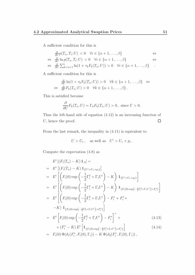
4.2 Approximated Analytical Swaption Prices 51
A sufficient condition for this is
∂∂U
p(Tα, Ti;U) < 0 ∀i ∈ α+ 1, . . . , β ⇔⇔ ∂
∂Uln p(Tα, Ti;U) < 0 ∀i ∈ α + 1, . . . , β ⇔
⇔ ∂∂U
∑ik=α+1 ln(1 + τkFk(Tα;U)) > 0 ∀i ∈ α + 1, . . . , β .
A sufficient condition for this is
∂∂U
ln(1 + τkFk(Tα;U)) > 0 ∀k ∈ α + 1, . . . , β ⇔⇔ ∂
∂UFk(Tα;U) > 0 ∀k ∈ α+ 1, . . . , β .
This is satisfied because
∂
∂UFk(Tα;U) = ΓkFk(Tα;U) > 0 , since Γ > 0 .
Thus the left-hand side of equation (4.12) is an increasing function of
U , hence the proof.
From the last remark, the inequality in (4.11) is equivalent to
U > U∗ , as well as U i > U∗ + pi .
Compute the expectation (4.8) as
Ei [(Fi(Tα)−K)1A] =
= Ei[(Fi(Tα)−K)1U i>U∗+pi
]
= Ei
[(Fi(0) exp
(−1
2Γ2i + ΓiU
i
)−K
)1U i>U∗+pi
]
= Ei
[(Fi(0) exp
(−1
2Γ2i + ΓiU
i
)−K
)1Fi(0) exp(− 1
2Γ2i+ΓiU i)>F ∗
i
]
= Ei
[(Fi(0) exp
(−1
2Γ2i + ΓiU
i
)− F ∗
i + F ∗i +
−K) 1Fi(0) exp(− 12Γ2γ+ΓiU i)>F ∗
i
]
= Ei
[Fi(0) exp
(−1
2Γ2i + ΓiU
i
)− F ∗
i
]++ (4.13)
+ (F ∗i −K)Ei
[1Fi(0) exp(− 1
2Γ2i+ΓiU i)>F ∗
i
](4.14)
= Fi(0) Φ(d1(F∗i , Fi(0),Γi))−K Φ(d2(F
∗i , Fi(0),Γi)) ,

52 4. Pricing of Swaptions in the LMM
where
F ∗i := Fi(0) exp
(−1
2Γ2i + ΓiU∗ + pi
)
and the last formula is obtained from the previous as:
(4.13) =
∫
D
(Fi(0) exp
(−1
2Γ2i + Γix
)− F ∗
i
) exp(−x2
2
)
√2π
dx
=
∫
D
(Fi(0) exp
(−(x− Γi)
2
2
)− F ∗
i exp
(−x2
2
))1√2π
dx ,
with D := Fi(0) exp(−1
2Γ2i + Γix
)> F ∗
i
= lnFi(0)− 12Γ2i + Γix > lnF ∗
i
= x >ln
F∗
iFi(0)
+ 12Γ2i
Γi = z >
lnF∗
iFi(0)
− 12Γ2i
Γi
⇒ (4.13) = Fi(0) Φ
ln Fi(0)
F ∗
i+ 1
2Γ2i
Γi
− F ∗
i Φ
ln Fi(0)
F ∗
i− 1
2Γ2i
Γi
;
(4.14) = (F ∗i −K)
∫
D
exp
(−x2
2
)1√2π
dx
= (F ∗i −K)Φ
ln Fi(0)
F ∗
i− 1
2Γ2i
Γi
.
Eventually we have an analytical formula that requires only a root-searching
procedure to find U∗ .
Proposition 4.2.1 (Brace’s rank-one formula). The approximated price of
a Tα × (Tβ − Tα) payer swaption is given by
β∑
i=α+1
τi p(0, Ti) [Fi(0) Φ(Γi − U∗ − pi)−K Φ(−U∗ − pi)] . (4.15)
Proof.
d1(F∗i , Fi(0),Γi) =
lnFi(0)
F∗
i+ 1
2Γ2i
Γi=
− ln(exp(− 12Γ2i+Γi(U∗+pi)))+ 1
2Γ2i
Γi
=12Γ2i−Γi(U∗+pi)+
12Γ2i
Γi= Γi − U∗ − pi .

4.2 Approximated Analytical Swaption Prices 53
Analogously
d2(F∗i , Fi(0),Γi) = U∗ − pi .
4.2.2 Rank-r analytical Swaption prices
The approach is the same as in the rank-one case and the first two steps
still hold in the extended rank-r case.
Then define a rank-r approximation of V as follows: V ≈ V r := ΓΓ′ ,
where Γ :=[√
λ1(V )e1(V )√
λ2(V )e2(V ) · · ·√λr(V )er(V )
].
Thus
Xγ Qγ
∼ N (0, V r)
with components given by
Xγi = Γ(i)U
γ , where Uγ Qγ
∼ N (0, Ir)
and Γ(i) is the ith row of Γ .
Typically it suffices r << β − α .
Formulae and definitions in (4.10) still hold by replacing ΓkΓj with Γ(k)Γ(j)′.
Under the same adjustments, the following formulae still hold up to the
observation (4.12), but here U , the qγ,k’s and the pγ’s are r-vectors.
Now the equation (4.12) was found (Brace,1997) to describe with a fair
approximation a hyperplane:
U1 = s1 +
r∑
k=2
skUk .
Remark 7. The set A can be rewritten as follows:
A =
U ∈ R
r : U1 > s1 +r∑
k=2
skUk
. (4.16)
Indeed, exactly as in the rank-one case, the partial derivative with respect
to U1 of the left-hand side of the equation corresponding to (4.12) is shown
to be positive.

54 4. Pricing of Swaptions in the LMM
Remark 8. The set A can be expressed in terms of U i as follows:
A =U i ∈ R
r : wU i > s∗i, (4.17)
where
w :=[1 −s2 · · · −sr
], s∗i := s1 + (pi)1 −
r∑
k=2
sk(pi)k .
Proof of (4.17). From (4.16) and U i = U + pi, we have
A =
U i ∈ R
r : U i1 −
r∑
k=2
skUik > s1 + (pi)1 −
r∑
k=2
sk(pi)k
.
Eventually, compute the expectation (4.8) as:
Ei [(Fi(Tα)−K)1A] =
= Ei[(Fi(Tα)−K)1wU i>s∗i
]
= Ei
[(Fi(0) exp
(Γ(i)U
i − 1
2|Γ(i)|2
)−K
)1wU i>s∗i
]
= Fi(0)Ei
[exp
(Γ(i)U
i − 1
2|Γ(i)|2
)1wU i>s∗i
]+KEi
[1wU i>s∗i
]
= Fi(0)Ei
[1w
(
U i+Γ∗
(i)
)
>s∗i
]−K Φ
(− s∗i|w|
)(4.18)
= Fi(0) Φ
(−s∗i − wΓ∗
(i)
|w|
)−K Φ
(− s∗i|w|
). (4.19)
Here, (4.18) follows from the first piece of the previous sum by applying the
property
Ei
[exp
(b′U i − 1
2b′b
)g(U i)
]= Ei
[g(U i + b)
],
which holds because
Ei[exp
(b′U i − 1
2b′b)g(U i)
]=
∫Rr e
b′u− 12b′bg(u)e−
12u′u 1√
(2π)rdu
=∫Rr e
− 12(u−b)′(u−b) g(u)√
(2π)rdu
(c.o.v. z = u− b) =∫Rr e
z′zg(z + b) 1√(2π)r
dz
= Ei [g(U i + b)] .

4.2 Approximated Analytical Swaption Prices 55
Instead, (4.19) follows from the second summand by exploiting the fact that
U i Qi
∼ N (0, Ir) ⇔ (U i)jQi
∼ N (0, 1) ∀j ∈ 1, . . . , r and (U i)j=1,...,r
are stochastically independent,
thus Z =wU i
|w| =
r∑j=1
wj(Ui)j
√r∑
j=1
w2j
=⇒ ZQi
∼ N (0, 1) .
Proposition 4.2.2 (Brace’s rank-r formula). The approximated price of a
Tα × (Tβ − Tα) payer swaption is given by
β∑
i=α+1
τi p(0, Ti)
[Fi(0) Φ
(−s∗i − wΓ(i)′
|w|
)−K Φ
(− s∗i|w|
)]. (4.20)
This analytical formula requires only 2r− 1 root-searching procedures to
find s1, . . . , sr, that can proceed according to the following:
• Solve numerically eq. (4.12) with U = [α1 0 · · ·0]′ , then s1 = α1 .
• Solve eq. (4.12) with U = [α−2 − 1
20 · · ·0]′ and with U = [α+
2120 · · ·0]′ ,
then s2 = α+2 − α−
2 .
• For k = 3, . . . , r solve eq. (4.12) with U = [α−k 0 · · ·
k
−12
0 · · ·0]′ and
with U = [α+k 0 · · ·
k120 · · ·0]′ , then sk = α+
k − α−k .
4.2.3 Rebonato’s approximation
In the LSM, the forward swap rate, which is always a martingal under
the measure Qα,β, has the dynamics
dSα,β(t) = σα,β(t)Sα,β(t)dWα,β(t) ,
where the volatility process σα,β is a deterministic function of time.
Instead, in the LMM, σα,β is a stochastic process, thus we can’t use this to

56 4. Pricing of Swaptions in the LMM
determine the Black swaption volatility vBα,β as
(vBα,β)2 =
1
Tα
∫ Tα
0
σ2α,β(t)dt , .
The goal is to find an approximated quantity vLMMα,β of vBα,β in the LMM.
Steps
• The forward swap rate can be obtained also by equating to zero the
expression of the swap price in the form of (1.5):
Sα,β(t) =
β∑
i=α+1
wi(t)Fi(t) , (4.21)
that looks like a weighted sum with weights
wi(t) :=τi p(t, Ti)
β∑k=α+1
τk p(t, Tk)
=
τii∏
j=α+1
11+τjFj(t)
β∑k=α+1
τkk∏
j=α+1
11+τjFj(t)
. (4.22)
However these ones are not really weights, because they depend on the
stochastic F’s.
According to empirical studies (both historically and through Monte
Carlo simulations), the variability of the wi’s is small compared to the
one of LIBOR rates, so that it makes sense to freeze the wi’s at their
initial values wi(0) .
• Thus approximate
Sα,β(t) ≈β∑
i=α+1
wi(0)Fi(t) .
Under any forward measure Qγ , γ ∈ 1, . . . ,M , its dynamics is
dSα,β(t) ≈β∑
i=α+1
wi(0)dFi(t) = (· · · )dt+β∑
i=α+1
wi(0)σi(t)Fi(t)dZγi (t)

4.2 Approximated Analytical Swaption Prices 57
and its quadratic variation process is
d < Sα,β, Sα,β >t = dSα,β(t)dSα,β(t)
≈β∑
i,j=α+1
wi(0)wj(0)σi(t)σj(t)Fi(t)Fj(t)ρi,jdt .
The approximated forward swap volatility is then given by
σ2α,β(t) =
d < lnSα,β, lnSα,β >t
dt=
1
dt
(dSα,β(t)
Sα,β(t)
)(dSα,β(t)
Sα,β(t)
)
≈
β∑i,j=α+1
wi(0)wj(0)σi(t)σj(t)Fi(t)Fj(t)ρi,j
S2α,β(t)
.
• A further approximation makes the quadratic variation of lnSα,β deter-
ministic, by freezing all the remained random variables, the F ’s (even
inside Sα,β), at time 0:
σ2α,β(t) ≈
β∑i,j=α+1
wi(0)wj(0)σi(t)σj(t)Fi(0)Fj(0)ρi,j
S2α,β(0)
.
The forward swap rate, that isn’t log-normal in the LMM, can thus be
approximated with a log-normal process:
dSα,β(t) ≈ σα,β(t)Sα,β(t)dWα,β(t) ,
where
σα,β(t) :=
√√√√√√
β∑i,j=α+1
wi(0)wj(0)σi(t)σj(t)Fi(0)Fj(0)ρi,j
S2α,β(0)
.
• Finally compute the swaption price through the Black’s formula.
Proposition 4.2.3 (Rebonato’s formula). The LMM Black-like swap-
tion volatility can be approximated by vLMMα,β , with
(vLMMα,β )2 :=
β∑
i,j=α+1
wi(0)wj(0)Fi(0)Fj(0)ρi,jTα S
2α,β(0)
∫ Tα
0
σi(t)σj(t)dt .

58 4. Pricing of Swaptions in the LMM
4.2.4 Hull and White’s approximation
The above procedure can be slightly improved by computing the dynamics
of the swap rate Sα,β(t) before freezing the w’s:
dSα,β(t) =
β∑
i=α+1
(wi(t)dFi(t) + Fi(t)dwi(t)) + (· · · )dt (4.23)
=
β∑
i,h=α+1
(wh(t)δi,h(t) + Fi(t)∂wi(t)
∂Fh
)dFh(t) + (· · · )dt ,(4.24)
where (4.23) is obtained by applying the Ito’s formula to Sα,β = Sα,β(t, F, w)
and (4.24) applying the Ito’s formula to wi = wi(t, F ).
Then, from (4.22), compute
∂wi(t)
∂Fh
=
wiτh
(β∑
k=h
τkk∏
j=α+1
11+τjFj(t)
− 1i≥h
)
(1 + τhFh(t))β∑
k=α+1
τkk∏
j=α+1
11+τjFj(t)
.
Proof.
∂wi(t)
∂Fh
=
♣, if i < h
♠, if i ≥ h ,
where
♣ =
−τii∏
r=α+1
11+τrFr(t)
·β∑
k=h
τkk∏
j=α+1
j 6=h
11+τjFj(t)
−τh(1+τhFh(t))2
(β∑
k=α+1
τkk∏
j=α+1
11+τjFj(t)
)2
=wiτh
(1 + τhFh(t))2β∑
k=α+1
τkk∏
j=α+1
11+τjFj(t)
·β∑
k=h
τk
k∏
j=α+1
j 6=h
1
1 + τjFj(t)
=wiτh
(1 + τhFh(t))β∑
k=α+1
τkk∏
j=α+1
11+τjFj(t)
·β∑
k=h
τk
k∏
j=α+1
1
1 + τjFj(t),

4.3 Example: computational results of the different methods ofswaption pricing 59
♠ =
τii∏
r=α+1r 6=h
11+τrFr(t)
−τh(1+τhFh(t))2
·β∑
k=α+1
τkk∏
j=α+1
11+τjFj(t)
(β∑
k=α+1
τkk∏
j=α+1
11+τjFj(t)
)2 +♣
= ♣− wiτh
(1 + τhFh(t))β∑
k=α+1
τkk∏
j=α+1
11+τjFj(t)
.
Hence the proof.
By denote
wh(t) := wh(t) +
β∑
i=α+1
Fi(t)∂wi(t)
∂Fh
,
the swap rate dynamics can be rewritten as
dSα,β(t) =
β∑
h=α+1
wh(t)dFh(t) + (· · · )dt .
Now, freeze all F ’s at their initial values in order to approximate
dSα,β(t) ≈β∑
h=α+1
wh(0)dFh(t) .
Finally, as in the Rebonato’s procedure, derive the volatility-like quantity
vLLMα,β to be entered in the Black’s formula for swaptions.
Proposition 4.2.4 (Hull and White’s formula). The LMM Black-like swap-
tion volatility can be better approximated by vLMMα,β , with
(vLMMα,β )2 :=
β∑
i,j=α+1
wi(0)wj(0)Fi(0)Fj(0)ρi,jTα S
2α,β(0)
∫ Tα
0
σi(t)σj(t)dt .
4.3 Example: computational results of the
different methods of swaption pricing
We now show the results we obtain by implementing in Mathematica all
the different methods we presented above to price the swaptions in the LMM.

60 4. Pricing of Swaptions in the LMM
We started from an annual tenor structure
T0 = 1y, . . . , T49 = 50y
and with the market quotes for the spot-starting swap rates (i.e. where the
first reset date is the day of valuation, i.e. the 26th. of April, 2011)
S−1,0(0), S−1,1(0), . . . , S−1,49(0) ,
from which we recover through a bootstrapping procedure and a log-linear
interpolation, the zero-bond curve shown in Figure 4.1.
Out[126]=
10 20 30 40 50T
0.2
0.4
0.6
0.8
1.0
pH0,TL
Figure 4.1: Zero-bond curve obtained from market data in April 26,2011.
Furthermore, as other inputs to our functions, we have:
- an historical correlation matrix obtained by market data spanning the
year before March 29, 2001, and calibrated in the Schoenmakers and
Coffey’s three-parameter structure, shown later on in Figure 7.8 (we will
describe the topics of correlation modeling and historical correlation
respectively in Chapter 5 and in Section 7.1);
- the current quotes of LIBOR forward rates modeled, F1(0), . . . , F49(0),
obtained by their definition in terms of zero-coupon bond prices from
the curve in Figure 4.1;

4.3 Example: computational results of the different methods ofswaption pricing 61
- the forward volatilities obtained by calibrating the model to swaption
data with an extended triangular cascade calibration, which we will see
in Subsection 7.2.3.
We priced for example three payer swaptions with different maturities and
tenors and we display the results in Table 4.1.
Swaption with tenor Tα × Tβ − Tα and fixed rate K = 0.03
α = 5, β = 8 α = 5, β = 14 α = 13, β = 18
PSReb 0.0339696 0.100866 0.0467792
PSHW 0.0339599 0.100712 0.0468129
PSBr1 0.0339502 0.100645 0.0468045
PSBr3 0.0339492 0.100643 0.0468043
PSMC 0.0330096 0.100043 0.0467224
99% [0.0326904, 0.0333288] [0.099198, 0.100888] [0.0462018, 0.047243]
Table 4.1: Approximated prices of three payer swaptions with different ma-
turities and tenors, respectively by Rebonato’s, Hull and White’s, Brace’s
rank-1 and Brace’s rank-3 formulae and Monte Carlo simulation with 100000
scenarios and a time grid of step dt = 1360
y.
We can notice that, often, the four approximated analytical prices fall
all into the 99%-confidence interval provided by the Monte Carlo simulation.
Moreover, sometimes they seem to be grouped into two classes, one with the
Rebonato’s and Hull and White’s prices and another with the Braces’ prices,
among which we cannot state what is in general more accurate with respect
to the Monte Carlo result.

Chapter 5
Instantaneous Correlation
Modeling
In the LMM setting, it remains to define the instantaneous correlation
between all the forward LIBOR rates modeled. In fact, we derived the dy-
namics of the Fk’s as each dependent on a different random source Zk, that
is instantaneously correlated with the others.
Not all interest rate derivatives have the same dependence on correlations.
In the pricing of caps we have already observed that the payoff does not
depend on the joint dynamics of F ’s, unlike as the pricing of swaptions does,
depending on more than a single rate in a non-linear relation.
An appropriate correlation modeling can be important in the following step
of calibration to swaption prices and becomes definitely relevant when the
number of contracts to which the model has to be calibrated is large. The
challenge is to choose a structure both flexible enough to express a large
number of swaption prices and, at a same time, parsimonious enough to be
tractable.
The M-dimensional correlated Brownian motion Z is assumed to have an
associated constant correlation matrix ρ, which, recalling the Remark (14)
in Appendix C, is defined as
ρi,j := Corr(Zi(t), Zj(t)) =Cov(Zi(t), Zj(t))
Std(Zi(t))Std(Zj(t))=
< Zi, Zj >t
t
62

63
and it also holds that
ρ dt = d < Z >t= dZ(t)(dZ(t))′ ,
from which we call ρ the instantaneous correlation.
As far as the LMM is concerned, if we assume the volatilities of forward
rates constant on small time intervals of length ∆t, then we can consider
ρi,j a quantity roughly summarizing the ”degree of dependence” between
instantaneous changes of lnFi and lnFj:
< lnFi, lnFj >t=
∫ t
0
σi(s)σj(s)ρi,jds
⇒ ∆ < lnFi, lnFj >t=
∫ t+∆t
t
σi(s)σj(s)ρi,jds = σi(t)σj(t)ρi,j∆t
and
∆ < lnFi, lnFj >t√∆ < lnFi, lnFi >t ∆ < lnFj , lnFj >t
=σi(t)σj(t)ρi,j∆t√σ2i (t)σ
2j (t)(∆t)2
= ρi,j ,
so that the correlation between different forward rates is completely deter-
mined by the correlation between different scalar Brownian motions, as far
as the dynamics of the F ’s are given by the solutions of the SDEs in (2.2).
In the setting of the LMM, we stated that ρ is a square M-dimensional
matrix. There exist also low-factor models, i.e. driven by a d-dimensional
B.m. with d < M , which nevertheless have intrinsic problems to match
correlations between forward LIBOR rates realistically, therefore we consider
only M-dimensional structures.
Now, we recall the properties of a generic correlation matrix:
1. ρi,j = ρj,i ∀i, j (symmetry);
2. |ρi,j| ≤ 1 ∀i, j (normalization);
3. ρi,i = 1 ∀i (maximum correlation for maximum dependence);
4. x′ρx ≥ 0 ∀x (positive semidefinite matrix).

64 5. Instantaneous Correlation Modeling
Then, we describe the additional qualities that an instantaneous correlation
matrix associated with a LIBOR market model would have:
I. ρi,j ≥ 0 ∀i, j (positive correlations);
II. i 7→ ρi,j is decreasing ∀i ≥ j (joint movements of far away rates are
less correlated than ones of rates with close maturities);
III. i 7→ ρi+p,i is increasing ∀i , ∀ fixed p ∈ N (the larger the tenor, the
more correlated changes in equally spaced forward rates become).
A full-rank correlation matrix ρ has M(M−12
entries, thanks to the symmetry
and the 1’s in the diagonal. The high number of parameters can be a prob-
lem for practical purposes, e.g. it makes correlations to be irregular when
obtained by fitting swaption prices. There are two possible approaches to
this problem: to use parameterizations of a full-rank matrix or to reduce the
rank.
5.1 Full-rank parameterizations
A general full-rank semi-parametric structure, suggested by
Schoenmakers and Coffey (2000) is:
ρSC(c)i,j :=minci, cjmaxci, cj
, i, j = 1, . . . ,M , (5.1)
where c ∈ (RM)+ with components such that
1 = c1 < c2 < . . . < cM andc1
c2<
c2
c3< . . . <
cM−1
cM. (5.2)
Remark 9. ρSC(c) is determined by M − 1 parameters and satisfies all nec-
essary properties.
Proof. 1. follows directly from the definition;
2. , 3. , I. are obviously derived;

5.1 Full-rank parameterizations 65
4. is hard to prove;
II. ∀ fixed j , the map
i 7→ ρi,j =cj
ci, i ≥ j
is decreasing, because the ci’s are increasing;
III. For all i ∈ 1, . . . ,M − p :
ρSC(c)i+p,i =ci
ci+p=
p−1∏k=0
ci+kci+k+1
= cici+1
· A
where A :=p−1∏k=1
ci+kci+k+1
,
ρSC(c)i+1+p,i+1 =ci+1
ci+1+p=
p−1∏k=0
ci+1+kci+1+k+1
=p∏
k=1
ci+kci+k+1
= A · ci+p
ci+p+1,
but cici+1
< ci+p
ci+p+1from definition .
For this reason this form is called semi-parametric, in the sense that it
depends on M − 1 parameters, i.e. O(M), rather than O(M2) in case of a
non-parametric M ×M matrix, and consequently the parameter dimension
increase proportionally to the model dimension.
Let’s give an idea of the practical meaning of this structure, by showing
that there exists a class of random vectors which have a correlation matrix
satisfying the conditions (5.1)-(5.2).
Let c1 < c2 < . . . < cM be an arbitrary positive increasing sequence
with c1 = 1 and let Wi , i = 1, . . . ,M , be standard normally distributed
independent real r.v., then consider the random vector Y with components
Yi :=i∑
k=1
akWk ∼ N(0,
i∑
k=1
a2k
),
where
a1 = c1 = 1 and ai :=√c2i − c2i−1 for i = 2, . . . ,M .

66 5. Instantaneous Correlation Modeling
We rewrite Y as
Y = A ·W ∼ N (0, AA′) , (5.3)
where
A =
a1 0 · · · 0
a1 a2 0 · · · 0
......
. . .
...0
a1 a2 · · · aM
.
Then the covariance between Yi and Yj, for i ≤ j, is
Cov(Yi, Yj) = (AA′)i,j =
i∑
k=1
a2k = c2i ,
becausei∑
k=1
a2k = c21 +i∑
k=2
(c2k − c2k−1) = c2i .
Thus the correlation between them is
ρYi,Yj=
Cov(Yi, Yj)√i∑
k=1
a2k
√j∑
k=1
a2k
=c2ici cj
=ci
cj.
Hence it follows that the correlation matrix of Y is given by a structure of
kind (5.1)-(5.2), which consequently defines a real correlation matrix.
Theorem 5.1.1. Every correlation structure of type (5.1)-(5.2) can be equiv-
alently characterized in terms of a sequence of non-negative numbers,
∆2, . . . ,∆M , in the following representation:
ci = exp
(M∑
l=2
mini− 1, l− 1∆l
). (5.4)
Proof. We now prove the direction (5.1)-(5.2) ⇒ (5.4), whereas the converse
follows straightforwardly by checking (5.1)-(5.2) for the sequence (ci)i=1,...,M
defined by (5.4).
Define ξi := ln ci , 1 ≤ i ≤ M . Then ξ1 = 0, since c1 = 1, and for the
sequence (ξi) the following constraints yield:
ξi < ξi+1 , 1 ≤ i ≤ M − 1 ; (5.5)
ξi−1 + ξi+1 < 2ξi , 2 ≤ i ≤ M − 1 . (5.6)

5.1 Full-rank parameterizations 67
Indeed: (5.5) follows from the increasing monotony of both the sequence
(ci) and the function ln; (5.6) follows from the increasing monotony of the
function i 7→ cici+1
and consequently we have ln ci−1 − ln ci < ln ci − ln ci+1,
with again ln ր .
Now, introduce the new variables
∆i := 2ξi − ξi−1 − ξi+1 = (ξi − ξi−1)− (ξi+1 − ξi) ≥ 0 , (5.7)
for 2 ≤ i ≤ M − 1 ,
∆M := ξ2 −M−1∑
j=2
∆j . (5.8)
Hence, for 2 ≤ i ≤ M,
ξi = ξi − ξ1 =i∑
k=2
(ξk − ξk−1) =i∑
k=2
(ξk − ξk−1 − (ξ2 − ξ1) + ξ2 − ξ1)
= ξ2 +
i∑
k=3
(k−1∑
l=2
(ξl+1 − ξl − (ξl − ξl−1)) + ξ2
)
= (i− 1)ξ2 +
i∑
k=3
k−1∑
l=2
(ξl+1 − ξl − (ξl − ξl−1))
= (i− 1)ξ2 −i∑
k=3
k−1∑
l=2
∆l = (i− 1)ξ2 −i−1∑
l=2
i∑
k=l+1
∆l
= (i− 1)ξ2 −i−1∑
l=2
(i− l)∆l . (5.9)
It follows that
ξi+1 − ξi = ξ2 −i∑
l=2
(i+ 1− l)∆l +i−1∑
l=2
(i− l)∆l
= ξ2 −i∑
l=2
∆l − (l − l)∆l (5.10)
= ξ2 −i∑
l=2
∆l (5.11)
and the constraints (5.5)-(5.6) transform into
∆i ≥ 0 , 2 ≤ i ≤ M .

68 5. Instantaneous Correlation Modeling
Indeed:
(5.5), (5.11) ⇔ ξ2 >i∑
l=2
∆l , for 2 ≤ i ≤ M ;
(5.6), (5.11) ⇔i∑
l=2
∆l − ξ2 = ξi − ξi+1 > ξi−1 − ξi =i−1∑l=2
∆l − ξ2 for
2 ≤ i ≤ M − 1 ⇔ ∆i > 0 for 2 ≤ i ≤ M − 1 .
Then, by (5.8) and (5.9), we may express the ξ’s in terms of the new coordi-
nates ∆’s:
ξi = (i− 1)
M∑
l=2
∆l −i−1∑
l=2
(i− l)∆l
= i
(M∑
l=2
∆l −i−1∑
l=2
∆l
)−
M∑
l=2
∆l +i−1∑
l=2
l∆l
= (i− 1)
M∑
l=i
∆l −i−1∑
l=2
∆l −M∑
l=i
∆l +
i−1∑
l=2
l∆l
= (i− 1)M∑
l=i
∆l +i−1∑
l=2
(l − 1)∆l
=
M∑
l=2
min(i− 1), (l − 1)∆l .
Finally substitute the last equation in ci = exp(ξ) .
Remark 10. A correlation structure (5.1)-(5.2), by representation (5.4), yields
ρSCi,j = exp
(−
M∑
j=i+1
minl − i, j − i∆l
), i < j . (5.12)
Proof.
lnci
cj=
M∑
l=2
mini− 1, l − 1∆l −M∑
l=2
minj − 1, l − 1∆l ,
from which we have three cases:
mini− 1, l − 1 −minj − 1, l − 1 =
i− l, i ≤ l < j ;
i− j, i < j ≤ l ;
0, l ≤ i < j .

5.1 Full-rank parameterizations 69
Hence the proof.
From representation (5.4), particularly in the form (5.12), we can derive
conveniently various low parametric structures, presented below.
5.1.1 Low-parametric structures by Schoenmakers and
Coffey
By taking ∆2, . . . ,∆M−1 =: α ≥ 0 , and ∆M =: β ≥ 0 , we obtain the
following two-parameters form:
ρi,j = exp
[−|i− j|
(β + α
(M − i+ j + 1
2
))], i, j = 1, . . . ,M. (5.13)
Proof. For j < M :
ρi,j = exp
[−α
j∑
l=i+1
(l − i)− α
M−1∑
l=j+1
(j − i)− β(j − i)
]
= exp
[αi(M − 1− i)− α
j∑
l=i+1
l − αj(M − 1− j)− β(j − i)
]
= exp
[αi(M − 1− i)− α
(j(j + 1)
2− i(i+ 1)
2
)+
−α j(M − 1− j)− β(j − i)]
= exp
[αi
(M − 1
2− i
2
)− α
ij
2+ α
ij
2+
−α j
(M − 1
2− j
2
)− β(j − i)
]
= exp
[−(j − i)
(β + α
(M − i+ j + 1
2
))].

70 5. Instantaneous Correlation Modeling
For j = M :
ρi,M = exp
[−α
M−1∑
l=i+1
(l − i)− β(M − i)
]
= exp
[αi(M − 1− i)− α
((M − 1)M
2− i(i+ 1)
2
)− β(M − i)
]
= exp
[αi
(M − 1
2− i
2
)− αM
M − 1
2− β(M − i)
]
= exp
[(i−M)
(β + α
M − i− 1
2
)].
Notice that for α = 0 we get the simple correlation structure
ρi,j = e−β|i−j| , (5.14)
which is frequently used in practice in spite of the unrealistic fact that prop-
erty III. is not satisfied, as the sub-diagonals are constant rather than in-
creasing, i.e. the correlation between forward rates that are equally spaced
is constant in time.
Now introduce two new parameters:
ρ∞ := ρ1,M , and η :=α
2(M − 1)(M − 2) ,
where ρ∞ is the correlation between the farthest forward rates in the family
considered. Hence, by computing ln ρ∞ in terms of α, β and inverting the
definition of η , we obtain the old parameters in terms of the new ones as
β = −α
2(M − 2)− ln ρ∞
M − 1, α =
2η
(M − 1)(M − 2),
from which the form (5.13) transform into
ρi,j = exp
[− |i− j|M − 1
(− ln ρ∞ + η
M + 1− i− j
M − 2
)]. (5.15)
This re-parametrization improves the parameter stability: relatively small
movements in the c-sequence associated with (5.15), and consequently in the
correlations themselves, cause relatively small movements in the parameters
ρ∞ , η .

5.1 Full-rank parameterizations 71
Suppose M > 2 and take the ∆i following a straight line for i =
2, . . . ,M − 1 and choose one parameter for i = M . Precisely:
∆2 = α1 ≥ 0 , ∆M−1 = α2 ≥ 0 , ∆M = β ≥ 0 ,
and for i = 2, . . . ,M − 1 we have
∆i = α1M − i− 1
M − 3+ α2
i− 2
M − 3.
Indeed, the equation representing the line, neither vertical nor horizontal,
through the two distinct points (2, α1) and (M − 1, α2) is
∆i =α2 − α1
M − 1− 2(i− 2) + α1 ,
where the coordinates of the points are (i,∆i) for each i.
Then we get the following three-parameter form:
ρi,j = exp[−|i− j|
(β − α2
6M−18(i2 + j2 + ij − 6i− 6j − 3M2 + 15M − 7)+
+ α1
6M−18(i2 + j2 + ij − 3Mi− 3Mj + 3i+ 3j + 3M2 − 6M + 2)
)].
(5.16)
Notice that (5.16) collapses to (5.13) if α1 = α2 = α, in which case we would
have an horizontal line for the first M − 2 points.
In order to gain stability, as above, re-parameterize (5.16) by introducing
ρ∞ := ρ1,M , which yields
β = − ln ρ∞M − 1
− α1
6(M − 2)− α2
3(M − 2) ,
and by setting
α1 =6η1 − 2η2
(M − 1)(M − 2), α2 =
4η2(M − 1)(M − 2)
.
Then (5.16) becomes
ρi,j = exp[− |i−j|
M−1
(− ln ρ∞ + η1
i2+j2+ij−3Mi−3Mj+3i+3j+2M2−M−4(M−2)(M−3)
+
−η2i2+j2+ij−Mi−Mj−3i−3j+3M+2
(M−2)(M−3)
)].
(5.17)
Notice that for η1 = η2 =η
2the structure (5.17) collapses to (5.15) again, as
it is obvious.

72 5. Instantaneous Correlation Modeling
The calibration experiments of Schoenmakers and Coffey pointed out
that correlation structure (5.17) suits very well in practice. However, cali-
brating a three-parameter matrix takes longer than a two-parameter one.
Furthermore, the experiments reveal that η2 ≈ 0 in (5.17), i.e. the final
point of the straight line in the ∆’s is practically always close to 0. Thus we
may adopt the following computationally improved correlation structure:
ρi,j = exp[− |i−j|
M−1(− ln ρ∞+
+η i2+j2+ij−3Mi−3Mj+3i+3j+2M2−M−4(M−2)(M−3)
)],
(5.18)
where the characteristics are the same of (5.17) apart from setting
η2 = 0 , η := η1 .
Consider the sequence (ci) defined by
ci := eβ(i−1)α , 1 ≤ i ≤ M , β > 0 , 0 < α < 1 .
The associated ρ satisfies the assumptions of a correlation structure (5.1)-
(5.2). Indeed:
ln
(ci
ci+1
)= ln ci − ln ci+1 = β ((i− 1)α − iα) < β (iα − (i− 1)α)
because i 7→ iα is an increasing function but with decreasing slope.
Then, by the definitions (5.7)-(5.8) in the proof of Theorem 5.1.1, we get the
coordinates
∆i = 2β(i− 1)α − β(i− 2)α − βiα , 2 ≤ i ≤ 2M − 1 ,
∆M = β −M−1∑
l=2
∆l = β − β
M−1∑
l=2
(2(l − 1)α − (l − 2)α − lα)
= β (1 + (M − 1)α − 2(M − 2)α + (M − 2)α + 1− 2)
= β ((M − 1)α − (M − 2)α) ,
where ∆i > 0 for 2 ≤ i ≤ M , as it must be.
Then, by introducing ρ∞ := ρ1,M = 1cM
, we get the correlations
ρi,j = exp
[ln ρ∞
∣∣∣∣(
i− 1
m− 1
)α
−(
j − 1
m− 1
)α∣∣∣∣]. (5.19)

5.1 Full-rank parameterizations 73
The correlation structures (5.18) and (5.19) have similar properties, but cal-
ibration experiments of Schoenmakers and Coffey pointed out that (5.18)
performs a little better.
5.1.2 Classical two-parameter structure
ρi,j = ρ∞ + (1− ρ∞) exp (−β|i− j|) , β ≥ 0 , (5.20)
where ρ∞ represents only asymptotically the correlation between the farthest
forward rates in the family.
This formulation guarantees all the desirable properties apart from III., in
the sense that sub-diagonals are flat. Notice that for ρ∞ = 0 we get the
simple structure (5.14), again.
5.1.3 Rebonato’s three-parameter structure
Rebonato suggested the following perturbation of the classical structure:
ρi,j = ρ∞ + (1− ρ∞) exp [−|i− j| (β − αmaxi, j)] . (5.21)
This structure recovers the property III., in fact
i 7→ ρi,j = ρ∞ + (1− ρ∞) exp [−p (β − α(i+ p))]
is increasing for α > 0 . Thus it may produce realistic market correlations for
properly chosen ρ∞, β > 0 and small α > 0 . However, (5.21) does not fit in
the general form (5.1)-(5.2) and its (α, ρ∞, β) domain of positivity is not ex-
plicitly specified, hence it is not guaranteed to be a correlation structure. To
avoid this problem, at every step of a hypothetical calibration/optimization,
it must be verified that the resulting matrix is positive semi-definite, for ex-
ample through a constrained optimization. Furthermore for inappropriate
values of ρ∞, β and not small enough α , it may also happen that ρi,j > 1,
thus the (5.21) is a weak characterization as correlation’s parametrization.

74 5. Instantaneous Correlation Modeling
5.2 Reduced rank parameterizations
Given ρ a positive definite symmetric matrix, it can be rewritten as
ρ = P∆P ′ , (5.22)
where ∆ is the diagonal matrix of (positive) eigenvalues of ρ in decreasing
order and P the orthogonal matrix whose columns are the corresponding
eigenvectors. Indeed:
ρP = P∆ , and P−1 = P ′ .
Let Λ be the diagonal matrix whose entries are the square roots of the cor-
responding ones of ∆, i.e. ∆ = ΛΛ .
Then define C := PΛ in order to have
ρ = CC ′ , C ′C = ∆ .
The correlated M-dimensional Brownian motion is distributed as
dZ ∼ N (0, ρdt) ,
whereas the standard M-dimensional Brownian motion is
dW ∼ N (0, Idt) ,
but we can replace dZ with CdW , where ρ = CC ′ .
If rank ρ = r < M , there exist a r-rank M × r matrix B such that
ρ = BB′ , and dZ = BdW .
The advantage in this replacement is that now we have a r-dimensional ran-
dom shock, given by the r-dimensional standard B.m. W .
Even when ρ is a full rank matrix, we may try and mimic the decompo-
sition ρ = CC ′ with a r-rank M × r correlation matrix B, by introducing a
new noise correlation matrix ρB = BB′, with typically r << M .

5.2 Reduced rank parameterizations 75
5.2.1 Rebonato’s angles method
Consider the M × r matrix
B = (bi,j)i=1,...,Mj=1,...,r
,
where for i = 1, . . . ,M the i-th row of B is
bi,1 = cos θi,1
bi,k = cos θi,k sin θi,1 · · · sin θi,k−1 , 1 < k < r
bi,r = sin θi,1 · · · sin θi,r−1
(5.23)
Notice that
ρB := BB′
results a positive semi-definite matrix and all its diagonal terms are equal to
1, thus it is a possible correlation matrix.
The number of parameters of this r-factor structure is M(r − 1), thus
the angles parametrization is not necessarily reducing the dimension of the
problem. In fact keeping for instance full-rank ρ, i.e. r = M , the number
of parameters is then M(M − 1), that is twice the number of entries of a
generic correlation matrix. To avoid a such inconvenient we have to ask not
only r < M , but rather
r <<M + 1
2.
5.2.2 Reduced rank approximations of exogenous cor-
relation matrices
When the correlation matrix is given exogenously as an historical estima-
tion, instead of being a fitting parameter in the calibration to the swaption
market, it has full rank M . The following two methods deal only with this
kind of situation.
The target is to obtain an approximated r-rank correlation matrix ρ(r),
with r < M :
M-rank historical ρ −→ r-rank ρ(r) .
Two different approaches are presented below.

76 5. Instantaneous Correlation Modeling
Eigenvalues zeroing with normalization
Consider the decomposition (5.22) and define Λ(r) as the r × r diagonal
matrix obtained from Λ by taking away theM−r smallest diagonal elements,
together with the corresponding dimensions, and P (r) as the M × r matrix
obtained from P by taking away the M − r corresponding columns.
Thus define B(r) := P (r)Λ(r), getting the matrix
ρ(r) := B(r)(B(r))′ ,
which is the best reduced rank approximation of ρ according to Frobenius
norm.
Remark 11. ρ(r) results positive semi-definite, but it does not features ones
in the diagonal.
The solution is to interpret ρ(r) as a covariance matrix and derive the
associated correlation matrix:
ρ(r)i,j :=
ρ(r)i,j√
ρ(r)i,i ρ
(r)j,j
.
Indeed, given a generic M-dimensional random variable X with covariance
matrix Σ = (σi,j) , which is a M × M positive semi-definite matrix, the
associated correlation matrix is
ρ = Λ−1ΣΛ−1 ,
where
Λ =
√σ1,1
. . .√σM,M
,
and σ2i = σi,i is the variance of the i-th component Xi, i = 1, . . . ,M .
Optimization on angles parametrization (Rebonato and Jakel, 1999)
Given the full rank correlation matrix ρ in input, we can find its r-rank
better approximation ρ(θ) = B(θ)B(θ)′ in terms of angles as in (5.23). Pre-

5.2 Reduced rank parameterizations 77
cisely, once defined the i-th row of B(θ) as
bi,1(θ) = cos θi,1
bi,k(θ) = cos θi,k sin θi,1 · · · sin θi,k−1 , 1 < k < r
bi,r(θ) = sin θi,1 · · · sin θi,k−1 ,
minimize with respect to (θ) the quantity
M∑
i,j=1
(|ρi,j − ρi,j(θ)|2) .
This method gives the optimal solution through an unconstrained optimiza-
tion.
Comparing the methods of eigenvalues zeroing and angles optimization,
we may see a noticeable better fit with the last one, despite a few seconds
of computation, with a low rank. This difference is going to attenuate by
increasing the rank.
In most situations a rank-4 approximation is satisfactory with both methods,
whereas in extreme cases we have to resort to a rank up the 7-th.

Chapter 6
Calibration of the LMM
6.1 Calibration of the LMM to Caplets
The LIBOR market model is calibrated to the most traded derivatives
among the liquid ones, namely the caplets, in an almost automatic way.
Indeed, the transition from caps to caplets is made by traders, then the
calibration of the LMM parameters to caps and floors results trivial, thanks
to the Proposition 2.1.1 and using market quoted volatilities.
Let assume that we are standing at time t = 0. Given an empirical term
structure of implied spot volatilities, from Proposition 2.1.1 it follows that
calibrating the model to caplets amounts to choose the deterministic LIBOR
volatilities of forward rates σ1, . . . , σM such that
v2Ti−capl =1
Ti−1
∫ Ti−1
0
σi(t)2dt , i = 1, . . . ,M . (6.1)
6.1.1 Parameterizations of Volatility of Forward Rates
The system (6.1) is highly undetermined, thus it needs structural assump-
tions about the shape of volatility functions. The most popular specifications
fall into two main categories: piecewise-constant functions, in which case the
σ’s are constant in each expiry-maturity time interval in which the corre-
sponding forward rates are alive, and functional parameterized forms, as
78

6.1 Calibration of the LMM to Caplets 79
shown below.
• General Piecewise-Constant volatilities (GPC):
σi(t) = σi,β(t) , 0 < t ≤ Ti−1 , (6.2)
where
β(t) = m if Tm−2 < t ≤ Tm−1 , m ≥ 1 . (6.3)
The index β(t) indicates the maturity of the first forward rate that has
not expired yet by time t. These σ’s can be organized in Table 6.1,
where we have the time intervals in the columns and the relative rates
in the rows.
t ∈ (0, T0] (T0, T1] (T1, T2] · · · (TM−2, TM−1]
F1(t) σ1,1 dead dead · · · dead
F2(t) σ2,1 σ2,2 dead · · · dead... · · · · · · · · · · · · · · ·
FM (t) σM,1 σM,2 σM,3 · · · σM,M
Table 6.1: General Piecewise-Constant volatilities.
To perform calibration, by inserting the expression (6.2) in the equa-
tion (6.1), we impose:
Ti−1v2Ti−capl =
∫ Ti−1
0
σ2i,β(t)dt =
1
Ti−1
i∑
j=1
τj−2,j−1σ2i,j , (6.4)
for i = 1, . . . ,M .
There exists multiple configurations that can fit caplets perfectly. In
fact:
√T0vT1−capl =
√(T0 − 0)σ1,1 ⇔ σ1,1 = vT1−capl
√T0σ
22,1 + (T1 − T0)σ2
2,2 =√T1vT2−capl
√T0σ
23,1 + (T1 − T0)σ2
3,2 + (T2 − T1)σ23,3 =
√T2vT3−capl
...

80 6. Calibration of the LMM
Then we can make some assumptions on this structure in order to
reduce the number of parameters.
• Piecewise-constant volatilities dependent only on the time to maturity
Ti − Tβ(t)−1 of corresponding forward rates:
σi(t) = σi,β(t) = ηi−(β(t)−1) , 0 < t ≤ Ti−1 . (6.5)
They are organized in Table 6.2.
t ∈ (0, T0] (T0, T1] (T1, T2] · · · (TM−2, TM−1]
F1(t) η1 dead dead · · · dead
F2(t) η2 η1 dead · · · dead... · · · · · · · · · · · · · · ·
FM (t) ηM ηM−1 ηM−2 · · · η1
Table 6.2: Time-to-maturity-dependent volatilities.
To perform calibration, by inserting the expression (6.5) in the equa-
tion (6.1), we impose:
Ti−1v2Ti−capl =
i∑
j=1
τj−2,j−1η2i−j+1 , (6.6)
for i = 1, . . . ,M .
In this case we can find the parameters η’s that exactly fit the mar-
ket caplets volatilities, being each of those obtained in terms of the
previous. In fact:
√(T0 − 0)η1 =
√T0vT1−capl ⇔ η1,1 = vT1−capl
√T0η
22 + (T1 − T0)η21 =
√T1vT2−capl ⇔
⇔ η2 =1√T0
√T1v
2T2−capl − (T1 − T0)η21

6.1 Calibration of the LMM to Caplets 81
√T0η
23 + (T1 − T0)η22 + (T2 − T1)η21 =
√T2vT3−capl ⇔
⇔ η3 =1√T0
√T2v
2T3−capl − (T1 − T0)η
22 − (T2 − T1)η
21
...
• Constant maturity-dependent volatilities:
σi(t) = σi,β(t) = si , 0 < t ≤ Ti−1 , (6.7)
as shown in Table 6.3.
t ∈ (0, T0] (T0, T1] (T1, T2] · · · (TM−2, TM−1]
F1(t) s1 dead dead · · · dead
F2(t) s2 s2 dead · · · dead... · · · · · · · · · · · · · · ·
FM (t) sM sM sM · · · sM
Table 6.3: Constant maturity-dependent volatilities.
To perform calibration, by inserting the expression (6.7) in the equa-
tion (6.1), we impose:
Ti−1v2Ti−capl = Ti−1s
2i ⇔ v2Ti−capl = s2i , (6.8)
for i = 1, . . . ,M .
Again, the parameters s’s can exactly fit the market caplets volatilities.
• Separable piecewise-constant volatilities, factorized as follows:
σi(t) = σi,β(t) = ΦiΨβ(t) , 0 < t ≤ Ti−1 , (6.9)
leading to Table 6.4.
This structure includes the one in (6.7) as a special case when all Ψ’s

82 6. Calibration of the LMM
t ∈ (0, T0] (T0, T1] (T1, T2] · · · (TM−2, TM−1]
F1(t) Φ1Ψ1 dead dead · · · dead
F2(t) Φ2Ψ1 Φ2Ψ2 dead · · · dead... · · · · · · · · · · · · · · ·
FM (t) ΦMΨ1 ΦMΨ2 ΦMΨ3 · · · ΦMΨM
Table 6.4: ΦiΨβ(t) structure
are equal to one. To perform calibration, by inserting (6.9) in (6.1), we
impose:
Ti−1v2Ti−capl = Φ2
i
i∑
j=1
τj−2,j−1Ψ2j , (6.10)
for i = 1, . . . ,M .
In this case, having read from the market the caplet volatilities vTi−capl =
vMKTi , the parameters Φ’s can be given in terms of the parameters Ψ’s
as
Φ2i =
Ti−1(vMKTi )2
i∑j=1
τj−2,j−1Ψ2j
.
• Separable piecewise-constant volatilities, factorized as follows:
σi(t) = σi,β(t) = ΦiΨi−(β(t)−1) , 0 < t ≤ Ti−1 , (6.11)
leading to Table 6.5.
This structure includes the one in (6.5) as a special case when all Φ’s
are equal to one. It concludes the piecewise-constant volatility models.
To perform calibration, by inserting (6.11) in (6.1), we impose:
Ti−1v2Ti−capl = Φ2
i
i∑
j=1
τj−2,j−1Ψ2i−j+1 , (6.12)
for i = 1, . . . ,M .
Similarly to the previous case, the parameters Φ’s can be given in terms

6.1 Calibration of the LMM to Caplets 83
t ∈ (0, T0] (T0, T1] (T1, T2] · · · (TM−2, TM−1]
F1(t) Φ1Ψ1 dead dead · · · dead
F2(t) Φ2Ψ2 Φ2Ψ1 dead · · · dead... · · · · · · · · · · · · · · ·
FM(t) ΦMΨM ΦMΨM−1 ΦMΨM−2 · · · ΦMΨ1
Table 6.5: ΦiΨi−(β(t)−1) structure
of the parameters Ψ’s as
Φ2i =
Ti−1(vMKTi )2
i∑j=1
τj−2,j−1Ψ2i−j+1
.
Even the continuous parameterizations have always been very popular.
The main examples are the following.
• Parametric linear exponential volatilities, analogue to form (6.5) :
σi(t) = Ψ(Ti−1 − t; a, b, c, d) := (a(Ti−1 − t) + d)e−b(Ti−1−t) + c . (6.13)
This time, in order to perform calibration, by inserting (6.13) in (6.1)
we obtain a continuous expression:
Ti−1v2Ti−capl = I2(Ti−1; a, b, c, d) , (6.14)
where
I2(Ti−1; a, b, c, d) :=
∫ Ti−1
0
([a(Ti−1 − t) + d]e−b(Ti−1−t) + c
)2dt .
The parameters a, b, c, d can be used to fit the market the caplet volatil-
ities through an optimization algorithm. This formulation can be per-
fected into the following richer parametric form.
• Parametric linear exponential volatilities, analogue to form (6.11) :
σi(t) = ΦiΨ(Ti−1 − t; a, b, c, d) = Φi
((a(Ti−1 − t) + d)e−b(Ti−1−t) + c
).
(6.15)

84 6. Calibration of the LMM
This form reduces to the previous by setting all the Φ’s to one.
In order to perform calibration, by inserting (6.15) in (6.1) we obtain:
Ti−1v2Ti−capl = ΦiI
2(Ti−1; a, b, c, d) . (6.16)
Now, having read from the market the caplet volatilities vTi−capl =
vMKTi , the parameters Φ’s can be given in terms of the parameters
a, b, c, d as:
Φ2i =
Ti−1(vMKTi )2
I2(Ti−1; a, b, c, d).
Notice that formulation (6.5) and (6.7) allow the complete determination
of the parameters in Tables 6.2 and 6.3 respectively, whereas with formu-
lations (6.2), (6.9) and (6.11) we cannot recover the whole tables of such
parameters, respectively Tables 6.1, 6.4 and 6.5, since we have more un-
known than equations. However, having parameters in excess can be helpful
when we have to calibrate the model, either to the swaptions together with
the caplets or only to the swaptions.
6.1.2 The Term Structure of Volatility
At each time Tj of the set of expiry-maturity dates of the LMM, the term
structure of volatility is the graph of the average volatilities V (Tj , Th−1) of
the forward rates Fh with fixing times Th−1 and maturities Th, in function of
expiry times Th−1. Namely, at time t = Tj , it is plotted the set of points
(Tj+1, V (Tj, Tj+1)), (Tj+2, V (Tj, Tj+2)), . . . , (TM−1, V (Tj, TM−1))
where, for h > j + 1,
V 2(Tj, Th−1) =1
τj,h−1
∫ Th−1
Tj
dFh(t)dFh(t)
Fh(t)Fh(t)=
1
τj,h−1
∫ Th−1
Tj
σ2h(t)dt .
In particular, the term structure of volatility at time t = 0 is
(T0, V (0, T0)), (T1, V (0, T1)), . . . , (TM−1, V (0, TM−1)) =
= (T0, vT1−capl), (T1, vT2−capl), . . . , (TM−1, vTM−capl) ,

6.1 Calibration of the LMM to Caplets 85
that is the market caplet volatility curve. A typical example of this curve
for annualized caplet volatilities from the Euro market, on May 4, 2011, is
shown in Figure 6.1.2.
In about the 80 percent of cases, the caplet volatility structure occurred
5 10 15 20 25expiry T j-1
0.05
0.10
0.15
0.20
0.25
0.30
vT j-capl
caplet volatilities
Figure 6.1: Term structure of volatility Tj 7→ vTj+1−capl from the Euro mar-
ket, on May 4, 2011; the resettlement dates T0, . . . , TM are annualized and
expressed in years.
with this initially humped shape. The short-term forward LIBOR rates (with
maturity maximum in a year) depends largely on the choices of the monetary
institutions and a bit on everything that happens on the market, e.g. even
when you read a news on a newspaper this can influence the rates’ trend,
therefore they have a high volatility. The long-term forward LIBOR rates
does not depend anymore neither on the expectations about the choices of
institutions like the BCE nor on minor news, therefore they have a lower
volatility. The little hump that is usually located between six months and
two or three years is due to the fact that the institutions of central banks
try to provide information in advance about their future actions, so that in
a very short time the volatility is relatively low, while the peak remains in
that period of time that is still influenced by actions and news but is out of
the near future in which we have the forecasts.

86 6. Calibration of the LMM
Up to July 2007 the very-short-term volatilities was very low, but from the
half of the same month, coinciding with the beginning of the crisis, these
volatilities have abruptly risen. As a consequence, in August 2007, mainly
in the USA and in GB, several banks registered big losses. Hence the central
banks inverted the way of working, by flooding the market with liquidity.
There are a few problems related to the choice of a parametrization for the
instantaneous volatilities of forward rates: different assumptions about those
imply different evolutions for the term structure of volatility. Moreover, dif-
ferent evolutions can change dramatically the price of some exotic products,
nevertheless they fit the whole structure of caplets today.
Let’s see the impact of different formulations by starting from the term struc-
ture of volatility today and getting its evolution in time.
• Formulation (6.5) gives
V 2(Tj, Th−1) =1
τj,h−1
h−1∑
k=j+1
τk−1,kη2h−k .
Assuming for simplicity that the year fractions are all equal to τ , we
have that τj,h−1 = (h − 1 − j)τ and another τ factorize out of the
summation, thus
V 2(Tj, Th−1) =1
(h− 1− j)
h−1∑
k=j+1
η2h−k ,
which implies that
V (Tj , Th−1) = V (Tj+1, Th) .
Therefore, the term structure of volatility simply shifts in time, i.e.
when moving from time Tj to time Tj+1 it moves from
(Tj+1, V (Tj, Tj+1)), (Tj+2, V (Tj, Tj+2)), . . . , (TM−1, V (Tj, TM−1))
to
(Tj+2, V (Tj, Tj+1)), (Tj+3, V (Tj, Tj+2)), . . . , (TM−1, V (Tj, TM−1)) .

6.1 Calibration of the LMM to Caplets 87
The shape of volatility structure remains exactly the same, except that
is shifted of one date in the future, consequently becomes shorter, in
the sense that the tail of the graph is cut away. An example of this kind
of evolution is shown in Figure 6.2, starting from the initial structure
of Figure 6.1.2.
5 10 15 20 25
0.05
0.10
0.15
0.20
0.25
0.30
Figure 6.2: Evolution of the term structure of volatility of Figure 6.1.2 ob-
tained by calibrating the parametrization (6.5).
Qualitatively, this is a desirable feature, since the actual shape of the
market term structure does not change too much over time. Anyway,
there remains the question of whether this formulation allows for a
humped structure to be fitted at the initial time. We note that the
map
Th−1 7→√
Th−1V (0, Th−1) =
√√√√τ
h−1∑
k=j+1
η2h−k
is increasing. On the other hand, we know that the market volatility
structure is decreasing following the hump, namely
V (0, Th−1) ≥ V (0, Th)
typically for Th larger that three or four years. Putting these two

88 6. Calibration of the LMM
constraints together we obtain:√Th−1V (0, Th−1) ≤
√ThV (0, Th)
V (0, Th−1) ≥ V (0, Th)⇒ 1 ≤ V (0,Th−1)
V (0,Th)≤√
Th
Th−1=√
hh−1
.
This means that for large h the obtained term structure gets almost
flat at the end, i.e.
V (0, Th−1) ≈ V (0, Th) for large h .
Thus we can use the formulation (6.5) unless the market term structure
is steeply decreasing also for large maturity.
• Formulation (6.7) gives
V 2(Tj , Th−1) = s2h .
Since this equality holds for all j = −1, 0, 1, . . . , h and the right member
is independent of j, the volatility term structure evolves simply by
cutting off the head. In particular, we move from the term structure
(Tj+1, sj+2)), (Tj+2, sj+3), . . . , (TM−1, sM) at time Tj
to
(Tj+2, sj+3)), (Tj+3, sj+4), . . . , (TM−1, sM) at time Tj+1 .
An example of this kind of evolution is shown in Figure 6.3, starting
from the initial structure of Figure 6.1.2.
This behaviour is not desirable, because even if the term structure
today features a hump around two years, this hump is disappearing in
the structure in three years.
• Formulation (6.9) gives
V 2(Tj , Th−1) =Φ2
h
τj,h−1
h∑
k=j+2
τk−2,k−1Ψ2k .
In this case it is hard to control the qualitative behaviour of the fu-
ture term structure of volatilities, because it depends on the particular
specification of both the Φ’s and the Ψ’s.

6.1 Calibration of the LMM to Caplets 89
5 10 15 20 25
0.05
0.10
0.15
0.20
0.25
0.30
Figure 6.3: Evolution of the term structure of volatility of Figure 6.1.2 ob-
tained with parametrization (6.7).
• Formulation (6.11) gives
V 2(Tj, Th−1) =Φ2
h
τj,h−1
h−1∑
k=j+1
τk−1,kΨ2h−k .
By assuming again τh−1,h = τ for all h = 0, . . . ,M − 1, it reduces to
V 2(Tj , Th−1) =Φ2
h
(h− 1− j)
h−1∑
k=j+1
Ψ2h−k .
Then, if the Φ’s are all equal, this formulation is analogous to the (6.5).
Therefore, keeping the Φ’s sufficiently close to each other, the quali-
tative behaviour of the future term structure of volatilities will not
be affected and the hump remains unchanged. This formulation is
considered the best among the piecewise-constant ones thanks to the
abundance of parameters together with the controllability of the future
evolution of the volatility structure.
• Formulation (6.13) gives
V 2(Tj, Th−1) =1
τj,h−1
∫ Th−1
Tj
Ψ(Th−1 − t; a, b, c, d)2dt . .

90 6. Calibration of the LMM
Being the analogous continuous version of the parametrization (6.5),
it maintains the shape of volatility structure as time passes, in par-
ticular its hump if initially present. Nevertheless, once again, it can’t
be used in the calibration if the initial structure is decreasing for large
maturities.
• Formulation (6.13) gives
V 2(Tj, Th−1) =Φh
τj,h−1
∫ Th−1
Tj
Ψ(Th−1 − t; a, b, c, d)2dt . .
Being the analogous continuous version of the parametrization (6.11),
if all the Φ’s are all close to each other the term structure maintains
its humped as time passes, if initially humped.

Chapter 7
Calibration of the LMM to
Swaptions
Since swaption prices are quoted in the market, calibrating the LIBOR
market model to swaptions means reducing the distance between the mar-
ket quotes and the prices obtained in the LMM, by working on the model
parameters. But it is not all. Indeed, there are two points of interest: the
computational cost and the financial plausibility. On the one hand, the step
of calibration comes before anything else, hence it cannot be a slow proce-
dure. On the other hand, in case we have to price other products that are
very distant from those to which we have calibrated the model, we may find
quite different values depending on which model’s parametrization we have
chosen.
In the LMM framework, the free parameters are those deriving from the
instantaneous correlation and the volatility parameterizations.
Generally, traders translate swaption prices into implied Black’s swaption
volatilities and organize them in a table where the rows are indexed by the
maturity time and the columns are indexed by the length of the underlying
swap. An example of such a table of swaption volatilities is shown in Fig-
ure 7.1.
We must be careful to the shift of indexes of the resettlement dates of the
91

92 7. Calibration of the LMM to Swaptions
1y 2y 3y 4y 5y 7y 10y1y 0.327 0.291 0.273 0.26 0.251 0.236 0.2212y 0.313 0.272 0.256 0.247 0.241 0.23 0.2163y 0.284 0.253 0.24 0.232 0.227 0.219 0.2074y 0.259 0.234 0.225 0.218 0.213 0.206 0.1985y 0.238 0.22 0.212 0.206 0.201 0.195 0.197y 0.207 0.197 0.191 0.187 0.183 0.178 0.17810y 0.175 0.171 0.167 0.165 0.164 0.164 0.16815y 0.16 0.164 0.165 0.167 0.168 0.172 0.17820y 0.18 0.186 0.188 0.191 0.193 0.198 0.201
Figure 7.1: Implied volatilities obtained by inverting the Black’s formula for
swaption, with swaption prices from the Euro market, May 4, 2011.
model T0, . . . , TM with respect to the corresponding times in years. For in-
stance, the first row in the above figure is related to 1 year = T0 , the second
row to 2 years = T1 , and so on.
Furthermore, a thing to be extremely careful is the problem of ”temporal
misalignments” in the swaption matrix, in the sense that it is not necessarily
uniformly updated. Indeed, although it is not stated, generally the most
liquid swaptions are updated regularly, whereas other entries of the matrix
refer to older market situations. This fact, together with the problem coming
from the missing data, can cause troubles in the calibration.
A calibration of the LMM exclusively to swaptions aims to incorporate
as much information as possible from the table of implied volatilities in the
model parameters. In this case we can choose any of the methods we have
seen in Chapter 4 to compute approximated swaption prices, then apply it to
price all the swaptions present in the market table and finally find the param-
eters that minimize the distance between the corresponding prices. Instead,
if we are going to calibrate the LMM both to caplets and to swaptions, we
will proceed analogously but carrying out an optimization on less (or nei-
ther) parameters, because we can recover one of them in terms of the others
from each implied caplet volatility, as we have seen in the different cases of
Subsection 6.1.1. Anyway, we would get a good compromise between fitting
(low errors) and gumption.

7.1 Historical instantaneous correlation 93
At this point, we have two possible ways of acting: to consider the instan-
taneous correlation either as input, estimated exogenously and introduced in
the calibration leaving free only the volatility parameters, or output, also
considered as fitting parameter, of the calibration.
7.1 Historical instantaneous correlation
The opportunity to introduce in the calibration a correlation matrix given
exogenously allows us to incorporate the behaviour of the real market rates in
our model and to unburden the optimization procedure. On the other hand,
however, historical estimations reflect some problems deriving from the data
sampling, e.g. outliers and non synchronous data. A way to tackle this unde-
sirable feature is to use parameterized correlation matrices approximating the
one estimated and preserving by construction the desired characteristics al-
ready described at the beginning of Chapter 5. In support of this, European
swaption prices are relatively insensitive to correlation details and a more
regular correlation structure can lead, through calibration, to more regular
volatilities and to a more stable evolution of the volatility term structure.
7.1.1 Historical estimation
Initially, we have to recover market quotations for interest rates, gener-
ally forward LIBOR or forward swap rates, over time. They are characterized
by a fixed time to maturity, contrarily to the forward rates modeled in the
LMM, which have a fixed maturity date.
Therefore, we must compute first the zero coupon bond prices from the mar-
ket rates, that will be in the form
p(t1, t1 + si) , p(t2, t2 + si) , . . . , p(tl, tl + si) (7.1)
for every time to maturity si and time tj of quotations, always expressed in
years. In particular, we consider daily quotations and, since the first forward
rate modeled expires in T0, i.e. in one year from today, we go back only one

94 7. Calibration of the LMM to Swaptions
year with the data. Then, we carry out a linear interpolation between the
logarithms of the bond prices in (7.1) as functions of the maturity for each
fixed evaluation time, in order to compute then the bond prices related to
the fixed maturities T0, . . . , TM , constituting the tenor structure of our LMM,
and valued on the dates of the quotations, i.e. sequences
p(t1, Ti) , p(t2, Ti) , . . . , p(tl, Ti) (7.2)
for every i = 0, . . . ,M − 1 . From these, we get the annual forward rates
F0, . . . , FM−1 valued daily from one year to date.
Notice that we loss the last forward rate FM in the historical estimation.
At this point, based on the Gaussian approximation
(ln(
F1(ti+1)F1(ti)
). . . ln
(FM−1(ti+1)FM−1(ti)
) )∼ N (µ, V ) ,
we use the following estimators for the mean and variance,
µi := 1l−1
l−1∑k=1
ln(
Fi(tk+1)
Fi(tk)
),
Vi,j := 1l−1
l−1∑k=1
(ln(
Fi(tk+1)
Fi(tk)
)− µi
)(ln(
Fj(tk+1)
Fj(tk)
)− µj
),
(7.3)
where l is the number of past evaluation times, so that our estimation of the
historical correlation matrix ρ has elements
ρi,j =Vi,j√Vi
√Vj
.
Example of Historical estimation
Below, are shown the results obtained by historical data spanning the
year before March 29, 2001. In particular, we start with a table of rates
quoted at times t1 = −1y, . . . , tl = 0 , l = 260 (daily quotations apart
from holidays), specifically the EURIBOR rates for expires in one year and
the forward swap rates for tenors of 2, . . . , 20 years from t = 0. Then, we

7.1 Historical instantaneous correlation 95
compute the bond prices by performing a bootstrap and, through a log-
linear interpolation, recover the same prices in the form of (7.1), with the
annualized tenor structure T0 = 1y, . . . , T19 = 20y . From these, we recover
the forward rates F ∗1 (ti), . . . , F
∗18(ti) for i = 1, . . . , l , and get the estimate,
following (7.3)-(7.3), for the correlations between them, shown in Figures 7.2
and 7.3.
Figure 7.2: Three-dimensional plot of correlations ρi,j from the estimated
matrix in Figure 7.3.
We must notice that the resulting ρ has the characteristics of a correlation
matrix but it does not satisfy the financial expected properties I, II and III.
As mentioned above, once we get the historical estimate, we could con-
sider a parametric correlation matrix that well approximates that estimate.
To do this, we have two possibilities:
• choose any of the parameterizations in Chapter 5 and minimize some
loss function of the distance between the parametric form and the es-
timate ρ;

96 7. Calibration of the LMM to Swaptions
• directly estimate the correlations in the Schoenmakers and Coffey’s
semi-parametric structure (5.1)-(5.2).

7.1
Histo
ricalinsta
ntaneouscorre
latio
n97
F1 F2 F3 F4 F5 F6 F7 F8 F9 F10 F11 F12 F13 F14 F15 F16 F17 F18F1 1.00 0.88 0.70 0.66 0.60 0.51 0.50 0.49 0.55 0.60 0.59 0.61 0.60 0.58 0.57 0.56 0.55 0.56F2 0.88 1.00 0.93 0.88 0.81 0.75 0.73 0.71 0.77 0.79 0.78 0.78 0.77 0.74 0.73 0.72 0.70 0.70F3 0.70 0.93 1.0 0.96 0.87 0.82 0.81 0.79 0.84 0.84 0.82 0.82 0.81 0.79 0.78 0.77 0.75 0.74F4 0.66 0.88 0.96 1.00 0.94 0.91 0.90 0.89 0.91 0.90 0.88 0.87 0.86 0.84 0.83 0.81 0.79 0.78F5 0.60 0.81 0.87 0.94 1.00 0.98 0.98 0.97 0.96 0.92 0.91 0.89 0.89 0.87 0.85 0.82 0.80 0.79F6 0.51 0.75 0.82 0.91 0.98 1.00 0.99 0.98 0.96 0.91 0.89 0.87 0.87 0.85 0.82 0.80 0.78 0.76F7 0.50 0.73 0.81 0.90 0.98 0.99 1.0 0.98 0.97 0.91 0.90 0.88 0.88 0.86 0.83 0.80 0.78 0.77F8 0.49 0.71 0.79 0.89 0.97 0.98 0.98 1.0 0.97 0.91 0.90 0.88 0.87 0.86 0.83 0.80 0.78 0.76F9 0.55 0.77 0.84 0.91 0.96 0.96 0.97 0.97 1.00 0.95 0.94 0.93 0.92 0.91 0.89 0.86 0.84 0.84F10 0.60 0.79 0.84 0.90 0.92 0.91 0.91 0.91 0.95 1.00 0.98 0.96 0.95 0.95 0.94 0.93 0.91 0.90F11 0.59 0.78 0.82 0.88 0.91 0.89 0.90 0.90 0.94 0.98 1.0 0.97 0.96 0.95 0.95 0.92 0.91 0.90F12 0.61 0.78 0.82 0.87 0.89 0.87 0.88 0.88 0.93 0.96 0.97 1.00 0.97 0.95 0.95 0.92 0.90 0.88F13 0.60 0.77 0.81 0.86 0.89 0.87 0.88 0.87 0.92 0.95 0.96 0.97 1.00 0.98 0.96 0.93 0.91 0.90F14 0.58 0.74 0.79 0.84 0.87 0.85 0.86 0.86 0.91 0.95 0.95 0.95 0.98 1.0 0.97 0.95 0.93 0.93F15 0.57 0.73 0.78 0.83 0.85 0.82 0.83 0.83 0.89 0.94 0.95 0.95 0.96 0.97 1.0 0.96 0.96 0.95F16 0.56 0.72 0.77 0.81 0.82 0.80 0.80 0.80 0.86 0.93 0.92 0.92 0.93 0.95 0.96 1.00 0.96 0.97F17 0.55 0.70 0.75 0.79 0.80 0.78 0.78 0.78 0.84 0.91 0.91 0.90 0.91 0.93 0.96 0.96 1.00 0.96F18 0.56 0.70 0.74 0.78 0.79 0.76 0.77 0.76 0.84 0.90 0.90 0.88 0.90 0.93 0.95 0.97 0.96 1.00
Figu
re7.3:
Estim
atedcorrelation
matrix
ρob
tained
byhistorical
data
from
theEuro
market,
March
29,2011.

98 7. Calibration of the LMM to Swaptions
Example of Historically Optimized Rebonato’s correlation
For example, by performing in Matlab an optimization on the fitting
parameters of Rebonato’s form in (5.21), i.e.
ρRebi,j = ρ∞ + (1− ρ∞) exp [−|i− j| (β − αmaxi, j)] ,
wanting to approximate the historical estimate, we have obtained the follow-
ing values:
α = 2.249 ∗ 10−14 , β = 0.0068 , ρ∞ = 0.146 ,
which give the Rebonato’s correlations in Figures 7.4 and 7.5, respectively
plotted in the three-dimensional space and in the matrix form.
Figure 7.4: Three-dimensional plot of correlations ρRebi,j (α, β, ρinf) with the
values above for the parameters.

7.1
Histo
ricalinsta
ntaneouscorre
latio
n99
F1 F2 F3 F4 F5 F6 F7 F8 F9 F10 F11 F12 F13 F14 F15 F16 F17 F18F1 1.00 0.99 0.99 0.98 0.98 0.97 0.97 0.96 0.95 0.95 0.94 0.94 0.93 0.93 0.92 0.92 0.91 0.91F2 0.99 1.00 0.99 0.99 0.98 0.98 0.97 0.97 0.96 0.95 0.95 0.94 0.94 0.93 0.93 0.92 0.92 0.91F3 0.99 0.99 1.00 0.99 0.99 0.98 0.98 0.97 0.97 0.96 0.95 0.95 0.94 0.94 0.93 0.93 0.92 0.92F4 0.98 0.99 0.99 1.00 0.99 0.99 0.98 0.98 0.97 0.97 0.96 0.95 0.95 0.94 0.94 0.93 0.93 0.92F5 0.98 0.98 0.99 0.99 1.00 0.99 0.99 0.98 0.98 0.97 0.97 0.96 0.95 0.95 0.94 0.94 0.93 0.93F6 0.97 0.98 0.98 0.99 0.99 1.00 0.99 0.99 0.98 0.98 0.97 0.97 0.96 0.95 0.95 0.94 0.94 0.93F7 0.97 0.97 0.98 0.98 0.99 0.99 1.00 0.99 0.99 0.98 0.98 0.97 0.97 0.96 0.95 0.95 0.94 0.94F8 0.96 0.97 0.97 0.98 0.98 0.99 0.99 1.00 0.99 0.99 0.98 0.98 0.97 0.97 0.96 0.95 0.95 0.94F9 0.95 0.96 0.97 0.97 0.98 0.98 0.99 0.99 1.00 0.99 0.99 0.98 0.98 0.97 0.97 0.96 0.95 0.95F10 0.95 0.95 0.96 0.97 0.97 0.98 0.98 0.99 0.99 1.00 0.99 0.99 0.98 0.98 0.97 0.97 0.96 0.95F11 0.94 0.95 0.95 0.96 0.97 0.97 0.98 0.98 0.99 0.99 1.00 0.99 0.99 0.98 0.98 0.97 0.97 0.96F12 0.94 0.94 0.95 0.95 0.96 0.97 0.97 0.98 0.98 0.99 0.99 1.00 0.99 0.99 0.98 0.98 0.97 0.97F13 0.93 0.94 0.94 0.95 0.95 0.96 0.97 0.97 0.98 0.98 0.99 0.99 1.00 0.99 0.99 0.98 0.98 0.97F14 0.93 0.93 0.94 0.94 0.95 0.95 0.96 0.97 0.97 0.98 0.98 0.99 0.99 1.00 0.99 0.99 0.98 0.98F15 0.92 0.93 0.93 0.94 0.94 0.95 0.95 0.96 0.97 0.97 0.98 0.98 0.99 0.99 1.00 0.99 0.99 0.98F16 0.92 0.92 0.93 0.93 0.94 0.94 0.95 0.95 0.96 0.97 0.97 0.98 0.98 0.99 0.99 1.00 0.99 0.99F17 0.91 0.92 0.92 0.93 0.93 0.94 0.94 0.95 0.95 0.96 0.97 0.97 0.98 0.98 0.99 0.99 1.00 0.99F18 0.91 0.91 0.92 0.92 0.93 0.93 0.94 0.94 0.95 0.95 0.96 0.97 0.97 0.98 0.98 0.99 0.99 1.00
Figu
re7.5:
Reb
onato’s
three-p
arameter
structu
reap
prox
imatin
gthehistor-
icallyestim
ationρfou
ndin
Figu
re7.3.

100 7. Calibration of the LMM to Swaptions
Example of Historically Estimated S. & C.’s semi-parametric cor-
relation
We start again from historical data spanning the past year before March
29, 2011, and we consider the table, obtained before, of historical forward
rates F ∗1 (ti), . . . , F
∗18(ti) for i = 1, . . . , l .
Now, for each time ti, i = 1, . . . , l , we consider the r.v. defined by
y∗j (ti) := lnF ∗j (ti+1)
F ∗j (ti)
, for j = 1, . . . , m , m = 18 .
Then, we assume the vector y∗(ti), having values in Rm, following the model
(5.3), that we rewrite in the following form:
y = A ·W = L · diag(a) ·W ∼ N (0, AA′) ,
where
A =
a1 0 · · · 0
a1 a2 0 · · · 0
......
. . .
...0
a1 a2 · · · am
, L =
1 0 · · · 0
1 1 0 · · · 0
......
. . .
...0
1 1 · · · 1
, a =
a1
a2...
am
.
By defining an auxiliary vector
w = diag(a) ·W ∼ N(0, diag
(a2))
,
where the square acts componentwise, we have
w = L−1 · y .
Since we have an historical set of vectors y∗(ti), for i = 1, . . . , l , which we
consider a sample of realizations of y, we obtain a consequent sample of
realizations of w. Then, we compute the sample covariance matrix of the
vector w, say C, being an estimate of the actual one diag (a2), thus we
estimate the vector a2 by extracting the diagonal from C, say a2. Finally,
we get the vector
c =
√L · a2 ,
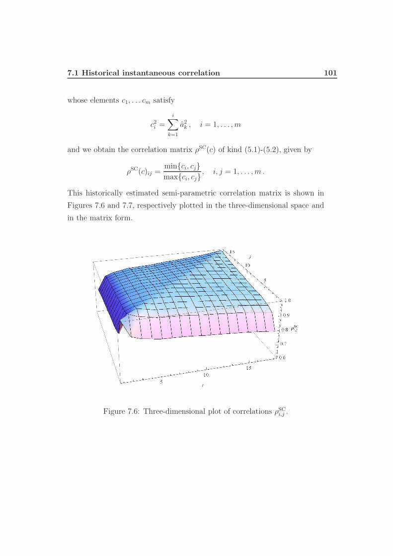
7.1 Historical instantaneous correlation 101
whose elements c1, . . . cm satisfy
c2i =
i∑
k=1
a2k , i = 1, . . . , m
and we obtain the correlation matrix ρSC(c) of kind (5.1)-(5.2), given by
ρSC(c)ij =minci, cjmaxci, cj
, i, j = 1, . . . , m .
This historically estimated semi-parametric correlation matrix is shown in
Figures 7.6 and 7.7, respectively plotted in the three-dimensional space and
in the matrix form.
Figure 7.6: Three-dimensional plot of correlations ρSCi,j .

102
7.Calib
ratio
nofth
eLM
Mto
Swaptio
ns
F1 F2 F3 F4 F5 F6 F7 F8 F9 F10 F11 F12 F13 F14 F15 F16 F17 F18F1 1.00 0.89 0.87 0.86 0.85 0.84 0.84 0.84 0.83 0.83 0.82 0.82 0.82 0.81 0.81 0.80 0.79 0.79F2 0.89 1.00 0.98 0.97 0.95 0.95 0.95 0.95 0.94 0.93 0.93 0.92 0.92 0.92 0.91 0.90 0.90 0.89F3 0.87 0.98 1.00 0.99 0.98 0.97 0.97 0.97 0.96 0.95 0.95 0.95 0.94 0.94 0.93 0.93 0.92 0.91F4 0.86 0.97 0.99 1.00 0.99 0.98 0.98 0.98 0.97 0.97 0.96 0.96 0.95 0.95 0.94 0.94 0.93 0.92F5 0.85 0.95 0.98 0.99 1.00 1.0 0.99 0.99 0.98 0.98 0.97 0.97 0.96 0.96 0.95 0.95 0.94 0.93F6 0.84 0.95 0.97 0.98 1.0 1.00 1.0 0.99 0.99 0.98 0.98 0.97 0.97 0.96 0.96 0.95 0.94 0.93F7 0.84 0.95 0.97 0.98 0.99 1.0 1.00 1.0 0.99 0.98 0.98 0.98 0.97 0.97 0.96 0.95 0.94 0.94F8 0.84 0.95 0.97 0.98 0.99 0.99 1.0 1.00 0.99 0.99 0.98 0.98 0.97 0.97 0.96 0.96 0.95 0.94F9 0.83 0.94 0.96 0.97 0.98 0.99 0.99 0.99 1.00 0.99 0.99 0.98 0.98 0.97 0.97 0.96 0.95 0.94F10 0.83 0.93 0.95 0.97 0.98 0.98 0.98 0.99 0.99 1.00 1.0 0.99 0.99 0.98 0.98 0.97 0.96 0.95F11 0.82 0.93 0.95 0.96 0.97 0.98 0.98 0.98 0.99 1.0 1.00 0.99 0.99 0.98 0.98 0.97 0.96 0.95F12 0.82 0.92 0.95 0.96 0.97 0.97 0.98 0.98 0.98 0.99 0.99 1.00 0.99 0.99 0.98 0.98 0.97 0.96F13 0.82 0.92 0.94 0.95 0.96 0.97 0.97 0.97 0.98 0.99 0.99 0.99 1.00 1.0 0.99 0.98 0.97 0.96F14 0.81 0.92 0.94 0.95 0.96 0.96 0.97 0.97 0.97 0.98 0.98 0.99 1.0 1.0 0.99 0.99 0.98 0.97F15 0.81 0.91 0.93 0.94 0.95 0.96 0.96 0.96 0.97 0.98 0.98 0.98 0.99 0.99 1.00 0.99 0.98 0.97F16 0.80 0.90 0.93 0.94 0.95 0.95 0.95 0.96 0.96 0.97 0.97 0.98 0.98 0.99 0.99 1.00 0.99 0.98F17 0.79 0.90 0.92 0.93 0.94 0.94 0.94 0.95 0.95 0.96 0.96 0.97 0.97 0.98 0.98 0.99 1.0 0.99F18 0.79 0.89 0.91 0.92 0.93 0.93 0.94 0.94 0.94 0.95 0.95 0.96 0.96 0.97 0.97 0.98 0.99 1.00
Figu
re7.7:
Schoenmakers
andCoff
ey’ssem
i-param
etriccorrelation
structu
re
estimated
byhistorical
data
fromtheEuro
market,
March
29,2011.
7.1 Historical instantaneous correlation 103
Example of Historically Optimized S. & C.’s three-parameter cor-
relation
By performing in Matlab an optimization on the fitting parameters of
Schoenmakers and Coffey’s three-parameter form in (5.17), i.e.
ρSCpari,j = exp
[− |i−j|
m−1
(− ln ρ∞ + η1
i2+j2+ij−3mi−3mj+3i+3j+2m2−m−4(m−2)(m−3)
+
−η2i2+j2+ij−mi−mj−3i−3j+3m+2
(m−2)(m−3)
)],
wanting to approximate the historical estimate ρ, we have obtained the fol-
lowing values:
η1 = 0.4856 , η2 = 0.00 , ln ρ∞ = −0.5395 ,
which give the correlations in Figures 7.4 and 7.5, respectively plotted in the
three-dimensional space and in the matrix form.
Figure 7.8: Three-dimensional plot of correlations ρSCpari,j .

104
7.Calib
ratio
nofth
eLM
Mto
Swaptio
ns
F1 F2 F3 F4 F5 F6 F7 F8 F9 F10 F11 F12 F13 F14 F15 F16 F17 F18F1 1.00 0.91 0.85 0.79 0.75 0.71 0.68 0.66 0.64 0.62 0.61 0.60 0.60 0.59 0.59 0.59 0.58 0.58F2 0.91 1.00 0.92 0.86 0.81 0.77 0.74 0.72 0.70 0.68 0.67 0.66 0.65 0.65 0.64 0.64 0.64 0.64F3 0.85 0.92 1.00 0.93 0.88 0.84 0.80 0.77 0.75 0.74 0.72 0.71 0.71 0.70 0.70 0.69 0.69 0.69F4 0.79 0.86 0.93 1.00 0.94 0.90 0.86 0.83 0.81 0.79 0.77 0.76 0.75 0.75 0.75 0.74 0.74 0.74F5 0.75 0.81 0.88 0.94 1.00 0.95 0.91 0.88 0.85 0.84 0.82 0.81 0.80 0.79 0.79 0.79 0.78 0.78F6 0.71 0.77 0.84 0.90 0.95 1.00 0.96 0.93 0.90 0.88 0.86 0.85 0.84 0.84 0.83 0.83 0.83 0.82F7 0.68 0.74 0.80 0.86 0.91 0.96 1.00 0.97 0.94 0.92 0.90 0.89 0.88 0.87 0.87 0.86 0.86 0.86F8 0.66 0.72 0.77 0.83 0.88 0.93 0.97 1.00 0.97 0.95 0.93 0.92 0.91 0.90 0.90 0.89 0.89 0.89F9 0.64 0.70 0.75 0.81 0.85 0.90 0.94 0.97 1.00 0.98 0.96 0.95 0.94 0.93 0.92 0.92 0.92 0.92F10 0.62 0.68 0.74 0.79 0.84 0.88 0.92 0.95 0.98 1.00 0.98 0.97 0.96 0.95 0.95 0.94 0.94 0.94F11 0.61 0.67 0.72 0.77 0.82 0.86 0.90 0.93 0.96 0.98 1.00 0.99 0.98 0.97 0.96 0.96 0.96 0.95F12 0.60 0.66 0.71 0.76 0.81 0.85 0.89 0.92 0.95 0.97 0.99 1.00 0.99 0.98 0.98 0.97 0.97 0.97F13 0.60 0.65 0.71 0.75 0.80 0.84 0.88 0.91 0.94 0.96 0.98 0.99 1.00 0.99 0.99 0.98 0.98 0.98F14 0.59 0.65 0.70 0.75 0.79 0.84 0.87 0.90 0.93 0.95 0.97 0.98 0.99 1.00 0.99 0.99 0.99 0.98F15 0.59 0.64 0.70 0.75 0.79 0.83 0.87 0.90 0.92 0.95 0.96 0.98 0.99 0.99 1.00 1.0 0.99 0.99F16 0.59 0.64 0.69 0.74 0.79 0.83 0.86 0.89 0.92 0.94 0.96 0.97 0.98 0.99 1.0 1.00 1.0 0.99F17 0.58 0.64 0.69 0.74 0.78 0.83 0.86 0.89 0.92 0.94 0.96 0.97 0.98 0.99 0.99 1.0 1.00 1.0F18 0.58 0.64 0.69 0.74 0.78 0.82 0.86 0.89 0.92 0.94 0.95 0.97 0.98 0.98 0.99 0.99 1.0 1.00
Figu
re7.9:
Schoenmakers
andCoff
ey’s
three-p
arameter
structu
reap
prox
i-
matin
gthehistorically
estimation
ρfou
ndin
Figu
re7.3.

7.2 Cascade Calibration 105
We denote the average squared relative error by MSE% and the average
simple relative error by ME%. In Table 7.1 we compare the errors charac-
terizing the three correlation get above, the Rebonato’s and Schoenmakers
and Coffey’s optimized three-parameter and the estimated Schoenmakers and
Coffey’s semi-parametric structure, in terms of the historical estimation.
ME% MSE%
Reb. three-par. 0.159833 0.246294
S. & C. semi-par. 0.136001 0.189073
S. & C. three-par. 0.0622644 0.0887776
Table 7.1: Average relative errors, both simple and squared, between histori-
cal estimation in Figures 7.3-7.2 and, respectively, the ones in Figures 7.5-7.4,
7.7-7.6 and 7.9-7.8.
7.2 Cascade Calibration
In Subsection 6.1.1 we presented some possible parameterizations of the
forward volatilities, that largely refer to the most general one, the GPC
formulation (6.2) shown in Table 6.1. This structure has a high number of
parameters, thus we then made some assumptions on it in order to reduce
the number of free parameters to be involved in an optimization algorithm of
the calibration. However, there exists an alternative method such that, given
exogenously the correlations, the calibration of the LMM to the swaptions
can be carried out through closed-form formulae. Substantially, we would
like to have a calibration that is:
- univocal, i.e. without all the indeterminacies seen in the calibration to
the caplets;
- exact, i.e. that avoids the problem of significant errors with respect to
the table of the market swaption volatilities;

106 7. Calibration of the LMM to Swaptions
- computationally efficient.
This method meets in a large part our expectations.
We assume the GPC volatility structure and we start from an historical
correlation matrix ρ and with the table of the swaption volatilities from the
market, denoting by Vα,β the Black volatility for the swaption with underlying
swap rate Sα,β.
By recalling the Rebonato’s formula for swaptions, the approximated
Black volatility in the LMM is
(vLMMα,β )2 :=
β∑
i,j=α+1
wi(0)wj(0)Fi(0)Fj(0)ρi,jTα Sα,β(0)2
∫ Tα
0
σi(t)σj(t)dt .
We apply this to the GPC formulation and equate it to the market swaption
volatility:
(Vα,β)2 ≈
β∑
i,j=α+1
wi(0)wj(0)Fi(0)Fj(0)ρi,jTα Sα,β(0)2
α∑
h=0
τhσi,h+1σ,j,h+1 , (7.4)
where we must remember that the w’s depend on the specific α, β considered.
The cascade calibration moves along the swaption table from left to right
and from top to down and we apply, at each step, the approximating for-
mula (7.4) to compute a new unknown volatility.
First, we analyze the simplest case of the calibration to the upper-left
triangular part of a swaption matrix providing all the market data involved,
which leads to sensible results, then the calibration to a rectangular sub-
matrix, again providing all the market volatilities involved. Finally, we con-
sider the extended triangular case in which we calibrate again to the upper-
left triangular part of a swaption matrix, where, however there are missing
data.
7.2.1 Triangular Cascade Calibration Algorithm
In this case we calibrate the GPC volatility formulation to the upper-left
triangular part of a swaption matrix where there are no missing data from

7.2 Cascade Calibration 107
the market. To give an overview of this procedure, in the Table 7.2 we show
the outcomes obtained by applying it to an example of just six swaptions.
Let’s see in detail how to proceed in this example. We start from the entry
Length 1year 2years 3years
Maturity
T0 = 1year V0,1 V0,2 V0,3
σ1,1 σ1,1 σ1,1
σ2,1 σ2,1
σ3,1
T1 = 2years V1,2 V1,3 –
σ2,1, σ2,2 σ2,1, σ2,2
σ3,1, σ3,2
T2 = 3years V2,3 – –
σ3,1, σ3,2, σ3,3
Table 7.2: Table summarizing the swaption volatilities to which we calibrate
the LMM through a triangular cascade calibration and the dependence of
the GPC forward volatilities on them, where the blue ones are the new pa-
rameters determined at each step.
V0,1 in position (1, 1), i.e. the swaption maturing in T0 e living up to T1, that
is an option on a single forward LIBOR rate collapsing to a spot LIBOR
rate, and the equation to solve has as unique unknown the volatility of F1
from now to T0 = 1year. Indeed:
S0,1(0) = w1(0)F1(0) ⇒ (V0,1)2 ≈ σ2
1,1 .
Hence the parameter σ1,1 is calibrated exactly.
Then we move to the entry (1, 2), V0,2, which involves the rates F1, F2
over the time from now to a year:
S0,2(0)2(V0,2)
2 ≈ w1(0)2F1(0)
2σ21,1 + w2(0)
2F2(0)2σ2
2,1 +
+2ρ1,2w1(0)F1(0)w2(0)F2(0)σ1,1σ2,1 ,

108 7. Calibration of the LMM to Swaptions
where the only unknown is σ2,1, which solves an algebraic second-order equa-
tion assuming existence and uniqueness of a positive solution.
Moving to the entry (1, 3), V0,3, the rate F3 is added among others, still
over [0, T0], and we have
S0,3(0)2(V0,3)
2 ≈ w1(0)2F1(0)
2σ21,1 + w2(0)
2F2(0)2σ2
2,1 + w3(0)2F3(0)2σ2
3,1 +
+2ρ1,2w1(0)F1(0)w2(0)F2(0)σ1,1σ2,1 +
+2ρ1,3w1(0)F1(0)w3(0)F3(0)σ1,1σ3,1 +
+2ρ2,3w2(0)F2(0)w3(0)F3(0)σ2,1σ3,1 ,
where the only unknown is σ3,1, which solves again a second-order equation,
by the same assumption of existence and uniqueness.
Now we move on the second row to the entry (2, 1), V1,2, where only F2 is
at stake but over the two time subintervals [0, T0], [T0, T1]. The formula (7.4)
gives
T1(V1,2)2 ≈ τ0σ
22,1 + τ1σ
22,2 ,
with the only unknown σ2,2.
Moving on the right to the entry (2, 2), V1,3, the formula (7.4) gives
T1S1,3(0)2(V1,3)
2 ≈ w2(0)2F2(0)
2(τ0σ22,1 + τ1σ
22,2) +
+w3(0)2F3(0)
2(τ0σ23,1 + τ1σ
23,2) +
+2ρ2,3w2(0)F2(0)w3(0)F3(0)(τ0σ2,1σ3,1 + τ1σ2,2σ3,2) ,
where the only unknown is σ3,2.
Finally, we move to the only entry (3, 1) on the third row, V2,3, where our
formula gives
T2(V2,3)2 ≈ τ0σ
23,1 + τ1σ
23,2 + τ2σ
23,3 ,
with the only unknown σ3,3.
Notice that each time we compute an only new parameter as a function
of a market swaption volatility and of the parameters previously found.
The procedure illustrated in the example above can be generalized in the
following scheme.

7.2 Cascade Calibration 109
Cascade Calibration Algorithm (CCA)
Brigo and Mercurio (2001,2002)
1. Select the dimension s of the swaption matrix that is of interest for the
calibration.
2. Set α = 0 .
3. Set β = α+ 1 .
4. Solve the following equation in σβ,α+1 :
Aα,βσ2β,α+1 +Bα,βσβ,α+1 + Cα,β = 0 , (7.5)
where
Aα,β = wβ(0)2Fβ(0)
2τα ,
Bα,β = 2
β−1∑
j=α+1
wβ(0)Fβ(0)wj(0)Fj(0) ρβ,j τα σj,α+1 ,
Cα,β =
β−1∑
i,j=α+1
wi(0)Fi(0)wj(0)Fj(0) ρi,j
α∑
h=0
τh σi,h+1 σj,h+1 +
+2
β−1∑
j=α+1
wβ(0)Fβ(0)wj(0)Fj(0) ρβ,j
α−1∑
h=0
τh σβ,h+1 σj,h+1 +
+wβ(0)2Fβ(0)
2α−1∑
h=0
τh σ2β,h+1 − Tα Sα,β(0)
2(Vα,β)2 .
Since Aα,β, Bα,β > 0, the equation (7.5) admits a unique positive solu-
tion, namely
σβ,α+1 =−Bα,β +
√B2
α,β − 4Aα,βCα,β
2Aα,β
,
if and only if Cα,β < 0.
5. Set β = α+ 1 ; if β ≤ s , go back to point 4, else set α = α + 1 .
6. If α < s , go back to point 3, else stop.

110 7. Calibration of the LMM to Swaptions
Practical experiences confirm that for non-pathological swaption data the
condition Cα,β < 0 is generally verified. Instead, in problematic situations, we
shall make some adjustments to this method, for example as in the extended
case. Notice that, in a triangular CCA of dimension s, the entries of the
swaption matrix involved are
(i, j) s.t. (i+ j) ≤ (s+ 1) ,
hence we calibrate the model to Black swaption volatilities
Vα,β s.t. 0 ≤ α ≤ s− 1, α + 1 ≤ β ≤ s .
Indeed: α = i− 1
β = α + j = i+ j − 1⇐⇒
i = α + 1
j = β − α .
This kind of calibration does not need further assumptions and it is indepen-
dent of the dimension s, provided all the market data involved, in the sense
that the output of the calibration to a sub-matrix of a swaption table V will
be a subset of the output of the calibration to V.
Example of a 5-dimensional Cascade Calibration
We applied the CCA to the 5 × 5 triangular sub-matrix of the implied
Black swaption volatilities shown in Figure 7.10, where we highlight the fact
that there are maturities with missing data by showing the corresponding
rows and columns empty. We chose s = 5, as it is the larger maturity with
no missing data before.
Again, we have to pay attention to the shift of the indexes of the resettlement
dates of the model with respect to the corresponding times in years.
The resulting calibrated forward volatilities are shown in Figure 7.11.
7.2.2 Rectangular Cascade Calibration Algorithm
If we want to calibrate the LMM to a whole rectangular swaption ma-
trix with all the entries provided by the market, we need to make some

7.2 Cascade Calibration 111
1 y 2 y 3 y 4 y 5 y 6 y 7 y 8 y 9 y 10 y
1 y 0.34 0.30 0.28 0.27 0.26 0.24 0.222 y 0.32 0.28 0.26 0.25 0.24 0.23 0.223 y 0.29 0.26 0.24 0.23 0.23 0.22 0.214 y 0.26 0.24 0.23 0.22 0.21 0.21 0.205 y 0.24 0.22 0.21 0.21 0.20 0.20 0.206 y7 y 0.21 0.20 0.19 0.19 0.18 0.18 0.188 y9 y10 y 0.18 0.17 0.17 0.17 0.17 0.17 0.1711 y12 y13 y14 y15 y 0.16 0.16 0.17 0.17 0.17 0.17 0.1816 y17 y18 y19 y20 y 0.18 0.18 0.19 0.19 0.19 0.20 0.21
Figure 7.10: Implied Black swaption volatilities, from the Euro market, April
26, 2011.
Σ =
0.342 0 0 0 00.274301 0.36172 0 0 00.264304 0.245348 0.344644 0 00.252787 0.24233 0.220029 0.311907 00.247875 0.231487 0.20753 0.191782 0.293202
Figure 7.11: Forward volatilities calibrated to the 5 × 5 sub-matrix of the
swaption table in Figure 7.10.
adjustments to the CCA algorithm, because, in general, there are no market
swaption tables large enough to contain our rectangular one in its upper-
triangular part.
By recalling the initial example of dimension s = 3, in the Table 7.3
we show the outcomes of the rectangular cascade calibration, involving nine
swaptions.
We can see how, in each entry of the last column except from the first, we

112 7. Calibration of the LMM to Swaptions
Length 1year 2years 3years
Maturity
T0 = 1year V0,1 V0,2 V0,3
σ1,1 σ1,1 σ1,1
σ2,1 σ2,1
σ3,1
T1 = 2years V1,2 V1,3 V1,4
σ2,1, σ2,2 σ2,1, σ2,2 σ2,1, σ2,2
σ3,1, σ3,2 σ3,1, σ3,2
σ4,1, σ4,2
T2 = 3years V2,3 V2,4 V2,5
σ3,1, σ3,2, σ3,3 σ3,1, σ3,2, σ3,3 σ3,1, σ3,2, σ3,3
σ4,1, σ4,2, σ4,3 σ4,1, σ4,2, σ4,3
σ5,1, σ5,2, σ5,3
Table 7.3: Table summarizing the swaption volatilities to which we calibrate
the LMM through a rectangular cascade calibration and the dependence
of the GPC forward volatilities on them, where the blue ones are the new
parameters determined at each step.
have multiple unknown forward volatilities. The easiest way to interrelate
them is to assume they are all equal and this assumption makes sense, because
the multiple unknowns are always volatilities of a single forward LIBOR rate
over a few adjacent intervals of time.
This method is described in detail in the following scheme.
Rectangular Cascade Calibration Algorithm (RCCA)
Brigo and Morini (2002), Morini (2002) The RCCA algorithm recovers the
first three points of the CCA algorithm, unchanged. At point 5 the new
condition for β becomes
β − α ≤ s .

7.2 Cascade Calibration 113
Moreover, in the case
β = s+ α ,
at point 4 we have to assume all the unknowns to be equal, i.e.
σβ,1 = σβ,2 = . . . σβ,α+1 .
Hence, instead of (7.5), the new equation to solve is
A∗α,βσ
2β,α+1 +B∗
α,βσβ,α+1 + C∗α,β = 0 , (7.6)
where
A∗α,β = wβ(0)
2Fβ(0)2
α∑
h=0
τh ,
B∗α,β = 2
β−1∑
j=α+1
wβ(0)Fβ(0)wj(0)Fj(0) ρβ,j τα σj,α+1 +
+2
β−1∑
j=α+1
wβ(0)Fβ(0)wj(0)Fj(0) ρβ,j
α−1∑
h=0
τh σj,h+1 ,
C∗α,β =
β−1∑
i,j=α+1
wi(0)Fi(0)wj(0)Fj(0) ρi,j
α∑
h=0
τh σi,h+1 σj,h+1 +
−Tα Sα,β(0)2(Vα,β)
2 .
Example of a 5-dimensional Rectangular Cascade Calibration
We applied the RCCA to the whole 5 × 5 sub-matrix of the implied
Black swaption volatilities shown in Figure 7.10 and the resulting calibrated
forward volatilities are shown in Figure 7.12.
7.2.3 Extended Triangular Cascade Calibration Algo-
rithm
In case we want to calibrate the model to a larger dimension of the swap-
tion table, we have to tackle the problem of missing data. We refer to the

114 7. Calibration of the LMM to Swaptions
Σ =
0.342 0 0 0 00.274301 0.36172 0 0 00.264304 0.245348 0.344644 0 00.252787 0.24233 0.220029 0.311907 00.247875 0.231487 0.20753 0.191782 0.2932020.233045 0.233045 0.199793 0.204828 0.1771520.220006 0.220006 0.220006 0.177201 0.1786260.206154 0.206154 0.206154 0.206154 0.179950.190429 0.190429 0.190429 0.190429 0.190429
Figure 7.12: Forward volatilities calibrated to the 5 × 5 sub-matrix of the
swaption table in Figure 7.10.
algorithm we are describing as to the ”ExtCCA Algorithm”.
It is essential to observe that the swaption volatility Vα,β, which is located
in the (α− 1, β − α) entry of the table, involves the forward volatilities
σi,j i=α+1,...,βj=1,...,α+1
.
Among these, as we are in the triangular case, the new unknown is always
σβ,α+1 .
Whenever the data Vα,β is not quoted by the market, we compute the
unknown forward volatility by means of the following devices:
σβ,α+1 = σβ−1,α+1, if α = 0;
σβ,α+1 =σβ,α+σβ−1,α
2, if α > 0.
Then, we create a fictitious data Vα,β, by the approximating formula (7.4),
using the σ’s already calibrated and the one defined above, in order to fill in
the incomplete market table.
Example of a 10 and a 15-dimensional ExtCCA
Firstly, we applied the ExtCCA to the 10 × 10 triangular sub-matrix of
the implied Black swaption volatilities shown in Figure 7.10 and the resulting
calibrated forward volatilities are shown in Figure 7.13.

7.2 Cascade Calibration 115
We exploit the calibrated σ’s to reconstruct the missing swaption volatil-
ities falling inside our triangular part of interest. Thus, the new obtained
swaption table is shown in Figure 7.14.
Then, we applied the ExtCCA to the largest 15 × 15 triangular matrix
deriving from the implied Black swaption volatilities shown in Figure 7.10
and the resulting calibrated forward volatilities are shown in Figure 7.15.
As above, we exploit the calibrated σ’s to reconstruct the missing swap-
tion volatilities falling inside our triangular part of interest, thus obtaining
the swaption table shown in Figure 7.16.
Conclusions about the Cascade Calibration
We may conclude by pointing out the main features of the cascade cali-
bration. Its positive aspects are:
• it makes use of the correlation matrix in input from a historical esti-
mation;
• it is a fast method, thanks to the analytical closed-form formulae;
• it is exact, i.e. if Rebonato’s approximation for the Black implied
volatility of swaptions is used, the swaption market prices are fitted
exactly;
• given correlation, it has a unique solution, under some homogeneity
assumptions;
• it induces a one-to-one relation between the model σ’s and the market
swaption volatilities.
However, on the other hand, we have encountered a few numerical problems,
for example the condition Cα,β < 0 is not always satisfied and some negative

116 7. Calibration of the LMM to Swaptions
or imaginary σ’s may come out. In particular, we came up against this
facts only in the last example of calibration, by carrying out an ExtCCA
with dimension s = 15, whereas is a too large because of the considerable
amount of missing data. Moreover, the temporal misalignments in the market
data provided by a single broker and the correlation coming from a different
calibration need more attention.

7.2
CascadeCalib
ratio
n117
Σ =
0.342 0 0 0 0 0 0 0 0 00.271535 0.363801 0 0 0 0 0 0 0 00.260861 0.244808 0.347639 0 0 0 0 0 0 00.249284 0.240942 0.221234 0.314935 0 0 0 0 0 00.244662 0.230049 0.208129 0.193539 0.295445 0 0 0 0 00.244662 0.217784 0.199226 0.205704 0.178541 0.236993 0 0 0 00.196503 0.220583 0.241022 0.180193 0.179805 0.179173 0.240164 0 0 00.196503 0.273879 0.247231 0.098049 0.168667 0.174236 0.139744 0.189954 0 00.196503 0.196503 0.207105 0.227168 0.133219 0.150943 0.201287 0.170515 0.180234 00.23603 0.216267 0.206385 0.163969 0.195569 0.164394 0.0756796 0.138483 0.154499 0.142269
Figu
re7.13:
Forw
ardvolatilities
calibrated
with
a10-d
imension
alExtC
CA
tothesw
aption
table
inFigu
re7.10.

118 7. Calibration of the LMM to Swaptions
1 y 2 y 3 y 4 y 5 y 6 y 7 y 8 y 9 y 10 y
1 y 0.34 0.30 0.28 0.27 0.26 0.25 0.24 0.23 0.22 0.222 y 0.32 0.28 0.26 0.25 0.24 0.23 0.23 0.23 0.22 0.223 y 0.29 0.26 0.24 0.23 0.23 0.23 0.22 0.22 0.214 y 0.26 0.24 0.23 0.22 0.21 0.21 0.21 0.205 y 0.24 0.22 0.21 0.21 0.20 0.20 0.20 0.206 y 0.21 0.21 0.20 0.20 0.197 y 0.21 0.20 0.19 0.19 0.18 0.18 0.188 y 0.19 0.19 0.189 y 0.19 0.1810 y 0.18 0.17 0.17 0.17 0.17 0.17 0.1711 y12 y13 y14 y15 y 0.16 0.16 0.17 0.17 0.17 0.17 0.1816 y17 y18 y19 y20 y 0.18 0.18 0.19 0.19 0.19 0.20 0.21
Figure 7.14: Black swaption volatilities partially reconstructed after a 10-
dimensional ExtCCA to the market swaption table in Figure 7.10.

7.2
CascadeCalib
ratio
n119
Σ =
0.342 0 0 0 0 0 0 0 0 0 0 0 0 0 00.271535 0.363801 0 0 0 0 0 0 0 0 0 0 0 0 00.260861 0.244808 0.347639 0 0 0 0 0 0 0 0 0 0 0 00.249284 0.240942 0.221234 0.314935 0 0 0 0 0 0 0 0 0 0 00.244662 0.230049 0.208129 0.193539 0.295445 0 0 0 0 0 0 0 0 0 00.244662 0.217784 0.199226 0.205704 0.178541 0.236993 0 0 0 0 0 0 0 0 00.196503 0.220583 0.241022 0.180193 0.179805 0.179173 0.240164 0 0 0 0 0 0 0 00.196503 0.273879 0.247231 0.098049 0.168667 0.174236 0.139744 0.189954 0 0 0 0 0 0 00.196503 0.196503 0.207105 0.227168 0.133219 0.150943 0.201287 0.170515 0.180234 0 0 0 0 0 00.23603 0.216267 0.206385 0.163969 0.195569 0.164394 0.0756796 0.138483 0.154499 0.142269 0 0 0 0 00.23603 0.166229 0.191248 0.198816 0.175855 0.185712 0.0453731 0.0605264 0.0995048 0.236383 0.189326 0 0 0 00.23603 0.23603 0.0946263 0.142937 0.170877 0.173366 0.179539 0.112456 0.0864912 0.191997 0.21419 0.201758 0 0 00.23603 0.23603 0.23603 0.190344 0.166641 0.168759 -0.0114842 0.0840273 0.0982416 0.0947651 0.143381 0.178785 0.190272 0 00.23603 0.23603 0.23603 0.23603 0.0610866 0.113864 0.141311 0.0649134 0.0744704 0.210479 0.152622 0.148002 0.163394 0.176833 0
0.23603 0.23603 0.23603 0.23603 0.23603 0.148558 0.131211 0.136261 0.100587 0.0875288 0.149004 0.150813 0.149407 0.1564 0. + 0.248824 ä
Figu
re7.15:
Forw
ardvolatilities
calibrated
with
a15-d
imension
alExtC
CA
tothesw
aption
table
inFigu
re7.10.

120
7.Calib
ratio
nofth
eLM
Mto
Swaptio
ns
1 y 2 y 3 y 4 y 5 y 6 y 7 y 8 y 9 y 10 y 11 y 12 y 13 y 14 y 15 y
1 y 0.34 0.30 0.28 0.27 0.26 0.25 0.24 0.23 0.22 0.22 0.22 0.22 0.22 0.22 0.222 y 0.32 0.28 0.26 0.25 0.24 0.23 0.23 0.23 0.22 0.22 0.22 0.22 0.22 0.223 y 0.29 0.26 0.24 0.23 0.23 0.23 0.22 0.22 0.21 0.21 0.21 0.21 0.214 y 0.26 0.24 0.23 0.22 0.21 0.21 0.21 0.21 0.20 0.20 0.20 0.205 y 0.24 0.22 0.21 0.21 0.20 0.20 0.20 0.19 0.20 0.20 0.206 y 0.21 0.21 0.20 0.20 0.19 0.19 0.19 0.19 0.19 0.197 y 0.21 0.20 0.19 0.19 0.18 0.18 0.18 0.18 0.18 0.188 y 0.19 0.19 0.18 0.18 0.17 0.17 0.17 0.189 y 0.19 0.18 0.17 0.17 0.17 0.17 0.1710 y 0.18 0.17 0.17 0.17 0.17 0.17 0.17 0.1711 y 0.17 0.17 0.17 0.17 0.1712 y 0.18 0.17 0.17 0.1713 y 0.17 0.17 0.1714 y 0.17 0.1715 y 0.16 0.16 0.17 0.17 0.17 0.17 0.1816 y17 y18 y19 y20 y 0.18 0.18 0.19 0.19 0.19 0.20 0.21
Figu
re7.16:
Black
swap
tionvolatilities
partially
reconstru
ctedafter
a15-
dim
ension
alExtC
CA
tothemarket
swap
tiontab
lein
Figu
re7.10.

Appendix A
Preliminary theory
Definition A.1. We define an N -dimensional Ito process any stochastic
process X = (Xt)t∈[0,T ] whose dynamics is given by
dXt = µtdt+ σtdWt
where W is a d-dimensional standard Brownian motion on (Ω,F , P, (Ft)),
µ, σ ∈ L2loc(Ω× [0, T ]) , µ having values in R
N and σ having values in RN×d .
Equivalently, in the integrated form, for i = 1, . . . , N the i-th component of
X follows:
X it = X i
0 +
∫ t
0
µisds+
d∑
j=1
∫ t
0
σi,js dW j
s .
Definition A.2. Given an N -dimensional Ito process X , the associated co-
variation process is the s.p. (< X,X >t)t∈[0,T ] with values in RN×d defined
by
< X i, Xj >t:= lim|Σ|→0
n∑
k=1
(X itk−X i
tk−1)(Xjtk−X
jtk−1) ,
where Σ = (0 = t0, . . . , tn = T ) | t0 < . . . < tn , n ∈ N .
Lemma A.0.1. With the notations above, let Ct = σtσ∗t , we have
< X i, Xj >t=
∫ t
0
C i,js ds , or equivalently d < X i, Xj >t= C
i,jt dt .
We use also the notation d < X i, Xj >t≡ (dX i) (dXj) .
121

122 A. Preliminary theory
Lemma A.0.2 (Ito’s formula). Given an N-dimensional Ito process with
dynamics
dXt = µtdt+ σtdWt
and a function F = F (t, x) ∈ C1,2([0, T ] × RN ) , then the s.p. Y defined by
Yt = F (t, Xt) is an Ito process with dynamics
dYt = ∂tF dt+∇F · dXt +1
2
N∑
i,j=1
∂xixjF d < X i, Xj >t , F ≡ F (t, Xt) .
Definition A.3. Given a d-dimensional B.m. W on (Ω,F , P, (Ft)), Z ∈ RN ,
µ : [0, T ] × RN → R
N , σ : [0, T ] × RN → R
N×d , the s.p. (Xt)t∈[0,T ] solves
the SDE with coefficients Z, µ, σ with respect to W if:
i) µ(t, Xt), σ(t, Xt) ∈ L2loc(Ω× [0, T ]) ;
ii) Xt = Z +∫ t
0µ(s,Xs)ds+
∫ t
0σ(s,Xs)dWs .
A statistical tool
Here, we give a basic and simple result that will be very useful as com-
monplace in pricing.
Lemma A.0.3. Let S be a random variable Log-Normally distributed with
mean m and variance Σ2, i.e. S = C eX with X ∼ N (m,Σ2) and C ∈ R,
and K be a real positive constant, K ∈ R+. Then:
E[(S −K)+
]= C e
Σ2
2+mΦ
(ln C
K+m+ Σ2
Σ
)−K Φ
(ln C
K+m
Σ
), (A.1)
where Φ is the cumulative distribution function for the N (0, 1) distribution.

123
Proof.
E[(S −K)+
]=
∫
R
maxC ex −K, 0 1√2πΣ
e−(x−m)2
2Σ2 dx
=1√2πΣ
∫
C ex>K(C ex −K) e−
(x−m)2
2Σ2 dx
=1√2πΣ
(∫
x>ln KCC ex e−
(x−m)2
2Σ2 dx−K
∫
x>ln KCe−
(x−m)2
2Σ2 dx
)
=1√2πΣ
(∫ +∞
ln KC
C e−1
2Σ2 (x2+m2−2xm−2xΣ2
dx+
−K
∫ +∞
ln KC
e−(x−m)2
2Σ2 dx
)
=1√2πΣ
(∫ +∞
ln KC
−m−Σ2
Σ
C e−z2
2 eΣ2
2+mΣ dz+ (A.2)
−K
∫ +∞
ln KC
−m
Σ
e−u2
2 Σ dx
)(A.3)
=1√2π
(C e
Σ2
2+m
∫ +∞
ln KC
−m−Σ2
Σ
e−z2
2 dz −K
∫ +∞
ln KC
−m
Σ
e−u2
2 dx
)
= C eΣ2
2+mΦ
(ln C
K+m+ Σ2
Σ
)−K Φ
(ln C
K+m
Σ
),
(A.4)
where the two summands in (A.2)-(A.3) are obtained respectively with the
two following changes of variable:
z =x−m− Σ2
Σ, u =
x−m
Σ.
Corollary A.0.4. If S is a random variable Log-Normally distributed with
mean −12Σ2 and variance Σ2, i.e. S = C eX with X ∼ N (−1
2Σ2,Σ2) and
C ∈ R, and K is a real positive constant, K ∈ R+, then:
E[(S −K)+
]= CΦ(d1(K,C,Σ2))−KΦ(d2(K,C,Σ2)) , (A.5)

124 A. Preliminary theory
where
d1(K,S,Σ2) :=ln(SK
)+ Σ2
2
Σ, (A.6)
d2(K,S,Σ2) := d1(K,C,Σ2)− Σ . (A.7)
Proof. It follows immediately from (A.1) by substituting m with −12Σ2.

Appendix B
Change of measure
The change of probability measure will be essential to deal with the con-
cept of martingale measure, which plays a central role in discrete as well as
continuous market modeling.
For mathematical reasons, financial prices are expressed in terms of ex-
pectation values, but if we use the probability measure of the real world we’ll
be in wrong, because the market would not be free of arbitrage opportunities.
Here comes the martingale measure, which leads to the risk-neutral price for
derivatives in an arbitrage-free market.
In the following, we are assuming to have a probability space (Ω,F , P, (Ft))
and, on this, a d-dimensional standard Brownian motion (Wt)t∈[0,T ].
Definition B.1. Let λ ∈ L2loc(Ω × [0, T ]) be a d-dimensional process, the
exponential martingale associated to λ is the s.p. Zλ defined by
Zλt = exp
(−∫ t
0
λs · dWs −1
2
∫ t
0
|λs|2ds)
, t ∈ [0, T ] .
Its dynamics is
dZλt = −Zλ
t λt · dWt .
Indeed, by Ito’s formula:
dZλt = Zλ
t
(−λt · dWt −
1
2|λt|2dt
)+
1
2Zλ
t |λt|2dt = −Zλt λt · dWt .
125

126 B. Change of measure
Since λ ∈ L2loc and Zλ is a continuous adapted process, than Zλλ ∈ L
2loc , so
that Zλ is a continuous local martingale. Moreover, being positive, it is also
a super-martingale, i.e.
E[Zλt ] ≤ [Zλ
0 ] = 1 , t ∈ [0, T ] .
There are some situations in which Zλ becomes a strict martingale.
Lemma B.0.5. If there exists a constant C such that
∫ T
0
|λt|2dt ≤ C a.s. ,
then the exponential martingale associated to λ, Zλ, is a strict martingale
such that
E
[sup
0≤t≤T
(Zλt )
p
]< ∞ , p ≥ 1 .
In particular Zλ ∈ Lp(Ω, P ) for every p ≥ 1 .
Theorem B.0.6 (Novikov condition). If λ ∈ L2loc(Ω× [0, T ]) is such that
E
[exp
(1
2
∫ T
0
|λs|2ds)]
< ∞ , (B.1)
then the the exponential martingale associated to λ, Zλ, is a strict martingale.
Let us endow the space (Ω,F , P ) with the Brownian filtration
FW = (FWt )t∈[0,T ] .
Theorem B.0.7 (Martingal representation). Let M = (Mt)t∈[0,T ] be
a FW -local martingale, then there exists a unique (just up to (m ⊗ P )-
equivalence) process u ∈ L2loc(FW ) such that
Mt = M0 +
∫ t
0
us · dWs , t ∈ [0, T ] .
The following basic theorem is used in the main topic of this chapter.

127
Theorem B.0.8 (Bayes’ Formula). Let P,Q be probability measures on (Ω,F),
with Q ≪F P , X ∈ L1(Ω, Q) , and G a sub-σ-algebra of F . Let L be the
Radon-Nikodym derivative of Q with respect to P , i.e.
Q(F ) =
∫
F
LdP , F ∈ F ,
denoted by L = dQ
dP= dQ
dP|F . Then we have
EQ[X | G] = EP [XL | G]EP [L | G] .
Proof. First denote B := EP [L|G] and prove that Q(B > 0) = 1 :
B = 0 ∈ G ⇒ Q(B = 0) =∫
B=0LdP =
∫
B=0BdP = 0 .
Then denote A := EQ[X|G] and prove that AB = EP [XL|G] : for all G ∈ G∫
G
AB dP =
∫
G
EP [AL|G] dP =
∫
G
AB dP =
∫
G
AdQ =
=
∫
G
EQ[X|G] dQ =
∫
G
X dQ =
∫
G
XLdP .
Thus, if Q is a probability measure on (Ω,F) defined by
ZλT =
dQ
dP, (B.2)
then, for every X ∈ L1(Ω, Q) we have
EQ[X | Ft] =EP [XZλ
T | Ft]
EP [ZλT | Ft]
, t ∈ [0, T ] .
Consequently we have the following lemma.
Lemma B.0.9. Let Zλ be a P -martingale and Q the probability measure on (Ω,F)
defined by (B.2). Then a process (Mt)t∈[0,T ] is a Q-martingale if and only if
(MtZλt )t∈[0,T ] is a P -martingale.

128 B. Change of measure
Theorem B.0.10 (Girsanov’s Theorem). Let Zλ be a P -martingale and
Q the probability measure on (Ω,F) defined by (B.2). Then the process W λ
defined by
W λt = Wt +
∫ t
0
λs · ds , t ∈ [0, T ] ,
is a Brownian motion on (Ω,F , Q, (Ft)) .
In financial applications, the processes playing the role of λ are often
bounded, so that the martingale property of Zλ follows from Lemma B.0.5.
Theorem B.0.11 (Change of drift). Let Q be a probability measure on (Ω,F)
equivalent to P , i.e. Q ∼ P . Then, the Radon-Nikodym derivative of Q with
respect to P is an exponential martingale:
dQ
dP|FW
t= Zλ
t , dZλt = −Zλ
t λt · dWt ,
with associated process λ ∈ L2loc(Ω× [0, T ]) , and the process W λ defined by
dWt = dW λt − λtdt (B.3)
is a Brownian motion on (Ω,F , Q, (Ft)) .
Proof. By denoting Zt :=dQ
dP|FW
t, we have
Zt = EP
[dQ
dP| FW
t
], t ∈ [0, T ] .
Indeed, for all A ∈ FWt ,
∫
A
ZtdP =
∫
A
dQ =
∫
A
dQ
dPdP .
Thus Z is a positive P -martingale, in fact Zt ≥ 0 ∀t ∈ [0, T ] and, ∀s < t ,
EP[Zt | FW
s
]= EP
[EP
[dQ
dP| FW
t
]| FW
s
]= EP
[dQ
dP| FW
s
]= Zs .
Then, by the martingale representation theorem B.0.7, there exists a unique
(P -a.s.) d-dimensional process u ∈ L2loc(FW ) such that
dZt = ut · dWt , or equivalently dZt = −Ztλt · dWt ,

129
having defined λ as the process
λt =ut
Zt
, t ∈ [0, T ] .
Since u ∈ L2loc and Z is a continuous adapted process, than λ ∈ L
2loc .
Hence Z is the exponential martingale associated with λ.
Finally, the Girsanov theorem states thatW λ in (B.3) is a B.m. on (Ω,F , Q, (Ft)) .
Remark 12. Let X be an N -dimensional Ito process of the form
dXt = µtdt+ σtdWt ,
µ having values in RN and σ having values in R
N×d .
Given Q ∼ P , then the Q-dynamics of X is
dXt = (µt − σtλt)dt+ σtdWλt .

Appendix C
Change of Measure with
Correlation in Arbitrage
Theory
In a continuous-time market model, where considering a probability space
(Ω,F , P ), the sources of risk are usually represented by a d-dimensional
correlated Brownian motion W = (W 1, . . . ,W d) on (Ω,F , P ), endowed with
the Brownian filtration (FWt )t∈[0,T ]. We consider the correlation constant in
time, thus define
Wt = A · Wt ,
where W is a standard d-dimensional Brownian motion and A = (Aij)i,j=1,...,d
is a non-singular d× d constant matrix.
We denote ρ := AA∗ and assume that, for i = 1, . . . , d ,
ρii =
d∑
j=1
(Aij)2 = 1 a.s.
Remark 13. For i = 1, . . . , d , W i is a standard 1-dimensional Brownian
motion.
Proof. All the properties of a real standard B.m. are verified:
130

131
1.
W i0 =
d∑
j=1
AijWj0 = 0 ;
2. W is a continuous adapted process on (Ω,F , P ) ;
3.
W it+h −W
jt =
d∑
j=1
Aij(W
jt+h − W
jt
)∼ N
(0, h
d∑
j=1
(Aij)2
)= N (0, h)
and(W i
t+h −Wjt
)does not depend on Ft.
The co-variation process of W has components given by
d < W i,W j >t= ρijdt , i, j = 1, . . . , d .
Notice that for all t it coincides with the covariance matrix of W . Indeed:
Wt ∼ N (0, t Idd) ⇒ Wt ∼ N (0, t AA′)
⇒ Cov(W it ,W
jt ) = ρij t =< W i,W j >t .
Remark 14. ρ is the correlation matrix of W (t) for each fixed time t.
Indeed,
Corr(W it ,W
jt ) =
Cov(W it ,W
jt )
Std(W it )Std(W
jt )
=ρij t√t√t= ρij ,
where we denote by Std(W it ) the standard deviation of W i
t , i.e.
Std(W it ) :=
√Cov(W i
t ,Wit ) .
When modeling a financial market, we assume the following hypothesis.

132 C. Change of Measure with Correlation in Arbitrage Theory
• There are N risky assets whose price process is S = (S1, . . . , SN) and
one locally no-risky asset B, that satisfy respectively the following dy-
namics:
dSit = µi
tSitdt+ σi
tSitdW
it , µi = bi +
(σi)2
2, i = 1, . . . , N (C.1)
and
dBt = rtBtdt , B0 = 1 , (C.2)
where b, r ∈ L1loc(Ω× [0, T ]) , σi positive ∈ L
2loc(Ω× [0, T ]) ∀i .
The dynamics in (C.1) derives from supposing
Sit = eX
it , dX i
t = bitdt+ σitdW
it , i = 1, . . . , N .
In fact, by Ito’s formula,
dSit = ∂xS
itdX
it+
1
2∂xxS
itd < X i, X i >t= Si
t(bitdt+σi
tdWit )+
1
2Sit(σ
i)2dt .
The integrated form of the solution of the SDE (C.1) is:
Sit = Si
0 exp
(∫ t
0
σisdW
is +
∫ t
0
(µis −
(σi)2
2
)ds
),
obtained by searching the two processes A,B such that
Sit = Si
0 exp(∫ t
0AsdW
is +
∫ t
0Bsds
), then by applying the Ito’s formula
and equating it to (C.1).
Notice that B, although representing a locally no-risky asset, is a
stochastic process, because r is a FW -progressively measurable pro-
cess. Anyway it has a smaller degree of randomness with respect to the
other assets, because it has bounded variation and consequently null
co-variation process. Indeed:
r ∈ L1loc ⇒ r(w) ∈ L1
[0,t] a.s. for w ∈ Ω
⇒∫ t
0rsds ∈ BV ⇒ exp
(∫ t
0rsds
)∈ BV .
• r and σ satisfy Lemma B.0.5.

133
• W is a d-dimensional Brownian motion with constant correlation ma-
trix ρ and d ≥ N .
Theorem C.0.12 (Change of drift with correlation). Let Q be a prob-
ability measure on (Ω,F) equivalent to P , i.e. Q ∼ P . Then, the Radon-
Nikodym derivative of Q with respect to P is an exponential martingale:
dQ
dP|FW
t= Zλ
t , dZλt = −Zλ
t λt · dWt ,
with associated process λ ∈ L2loc(Ω× [0, T ]) , and the s.p. W λ defined by
dWt = dW λt − ρλtdt (C.3)
is a Brownian motion on (Ω,F , Q, (FWt )) with correlation matrix ρ.
Proof. Let Zt = dQ
dP|FW
t, by the martingale representation theorem for the
standard B.m., there exists a unique (P -a.s.) d-dimensional process
λ ∈ L2loc(FW ) such that
dZt = −Ztλt · dW t = −Ztλt · (A−1dWt) = −Ztλt · dWt ,
where λt := (A−1)′λt . Notice that, by Ito’s formula,
Zt = exp
(−∫ t
0
λs · dW s −1
2
∫ t
0
|λs|2ds)
= exp
(−∫ t
0
< A∗λs, A−1dWs > −1
2
∫ t
0
< A∗λs, A∗λs > ds
)
= exp
(−∫ t
0
λs · dWs −1
2
∫ t
0
< ρλs, λs > ds
).
Then, by the Girsanov theorem, we have a standard Q-B.m. Wλ,
dWλ
t = dW t + λtdt , t ∈ [0, T ] . Multiplying by A this equation,
dW λt := AdW
λ
t = dWt + ρλtdt
is a correlated Q-B.m. with correlation matrix ρ.

134 C. Change of Measure with Correlation in Arbitrage Theory
Remark 15. Analogously to the standard case, let X be an N -dimensional
Ito process of the form
dXt = µtdt+ σtdWt ,
µ having values in RN and σ having values in R
N×d .
Given Q ∼ P , then the Q-dynamics of X is
dXt = (µt − σtρλt)dt+ σtdWλt .

Appendix D
Change of numeraire
Now we characterize the arbitrage-free financial markets by introducing
the previously mentioned equivalent martingale measure.
Definition D.1. An equivalent martingale measure (EMM ) Q with nu-
meraire B is a probability measure on (Ω,F) such that:
i) Q is equivalent to P ;
ii) the process of the discounted prices S = (St)t∈[0,T ] defined by
St =St
Bt
= e−∫ t0 rsdsSt , t ∈ [0, T ] ,
is a strict Q-martingale. In particular, the risk-neutral pricing formula
St = EQ[e−
∫ T
trsdsST | FW
t
], t ∈ [0, T ] ,
holds.
We consider a market model (S,B) of the form (C.1)-(C.2) and assume
that the class Q of the EMMs is not empty.
Definition D.2. Let Q ∈ Q be an EMM with numeraire B. A s.p. U is
called a Q-price process if:
i) U is strictly positive;
135

136 D. Change of numeraire
ii) the process of its discounted price U , Ut =Ut
Bt, t ∈ [0, T ] , is a strict
Q-martingale.
Practically, a Q-price process has all the features of a true price. The
martingale property leads to the risk-neutral pricing formula under Q:
Ut = EQ[D(t, T )UT | FW
t
], t ∈ [0, T ] ,
where D(t, T ) = Bt
BT= e−
∫ T
trsds is the standard discount factor.
Notice that any risky asset Si is a Q-price process.
The so called numeraire is a s.p. that represents a basic standard by
which the prices of all other assets are measured.
Definition D.3. Let U be a Q-price process, a probability measure QU on
(Ω,F) is called an EMM with numeraire U if:
i) QU is equivalent to P ;
ii) the processes of U -discounted prices St
Ut, Bt
Utare strict QU -martingales.
In particular, the risk-neutral pricing formulae
St = EQU [DU(t, T )ST | FW
t
], (D.1)
Bt = EQU [DU(t, T )BT | FW
t
], t ∈ [0, T ] (D.2)
hold, where DU(t, T ) = Ut
UTis the U -discount factor.
Theorem D.0.13. Let Q ∈ Q be an EMM with numeraire B and let U be a
Q-price process. Consider the probability measure QU on (Ω,F) defined by
dQU
dQ=
D(0, T )
DU(0, T )=
UTB0
BTU0
.
Then, for any X ∈ L1(Ω, Q), we have
EQ[D(t, T )X | FW
t
]= EQU [
DU(t, T )X | FWt
], t ∈ [0, T ] . (D.3)
In particular QU is an EMM with numeraire U and the risk-neutral price of
a European derivative X is equal to
EQU [DU(t, T )X | FW
t
], t ∈ [0, T ] .

137
Proof. Denote
Zt :=D(0, t)
DU(0, t)=
UtB0
BtU0, t ∈ [0, T ] .
Since U is a Q- price process,
Zt =B0
U0EQ
[UT
BT
| FWt
]= EQ
[D(0, T )
DU(0, T )| FW
t
]= EQ
[ZT | FW
t
],
hence Z is a strictly positive Q-martingale. Then, by the Bayes’ formula,
EQU [X | FW
t
]=
EQ[XZT | FWt ]
EQ[ZT | FWt ]
= EQ[X ZT
Zt| FW
t
]
= EQ[X
D(0,T )DU (0,T )
| FWt
],
(D.4)
becauseZT
Zt
=UTB0
BTU0
BtU0
UtB0=
UTB0
BTU0=
D(0, T )
DU(0, T ).
Now, taking (DU(t, T )X) in place of simply X in (D.4), we obtain
EQ[D(t, T )X | FW
t
]= EQ
[D(t, T )
DU(t, T )(DU(t, T )X) | FW
t
]
= EQU [DU(t, T )X | FW
t
].
Moreover QU ∼ Q, indeed ∃dQU
dQ, dQ
dQU > 0 , dQU
dQ, dQ
dQU ∈ L1, therefore QU ∼ P .
Finally, (D.3) prove (D.1) and (D.2).
Corollary D.0.14. Let U, V be Q-price processes with corresponding EMMs
QU , QV , respectively. Then, we have
dQV
dQU|FW
t =VtU0
UtV0
. (D.5)
Proof.
dQV
dQU|FW
t = EQU
[dQV
dQ
dQ
dQU| FW
t
]= EQU
[VTU0
UTV0
| FWt
]
=U0
V0EQU
[VT
UT
| FWt
]=
U0
V0
Vt
Ut
.
The last equality follows from Theorem D.0.13, since V is a Q-price process.

138 D. Change of numeraire
Forward measure
Let p(t, T ) be the price at time t, under a fixed EMM Q with numeraire
B, of the zero coupon bond with maturity T :
p(t, T ) = EQ[e−
∫ T
trsds | FW
t
], t ≤ T . (D.6)
Clearly p(t, T ) is a Q-price, because it is just defined through the risk neu-
tral pricing formula under the selected EMM Q. Thus there exist an EMM
associated with it, that is QT , called T -forward measure.
By Theorem D.0.13, the risk neutral price H of a European derivative X , at
time t, is equal to
Ht = EQT
[p(t, T )
p(T, T )X | FW
t
]= p(t, T )EQT [
X | FWt
]. (D.7)
This pricing formula in terms of a QT -expectation does not involve the
stochastic discount factor e−∫ T
trsds , as instead the Q-expectation does. On
the other hand, it needs to know the distribution ofX underQT , which can be
deduced by a change of drift (Theorem B.3) in terms of the Radon-Nikodym
derivative dQT
dQ= B0
p(0,T )BT(from (D.0.14)).
Now we move towards the cardinal theorem of the change of measure
induced by numeraires that are Ito processes.
Lemma D.0.15. Let U, V be two positive Ito processes of the form
dUt = (· · · )dt+ σUt · dWt ,
dVt = (· · · )dt+ σVt · dWt ,
where W is a correlated d-dimensional Brownian motion and
σU , σV ∈ L2loc(Ω× [0, T ];Rd) are the diffusion coefficients.
Then, Vt
Utis an Ito process of the form
dVt
Ut
= (· · · )dt+ Vt
Ut
(σVt
Vt
− σUt
Ut
)· dWt . (D.8)

139
Proof. Apply the Ito formula to the function F of the 2-dimensional Ito
process (U, V ), F (U, V ) = VU:
dVt
Ut
= − Vt
(Ut)2dUt +
dVt
Ut
+Vt
(Ut)3d < U, U >t −
1
(Ut)2d < U, V >t
= (· · · )dt− Vt
(Ut)2σUt · dWt +
1
Ut
σVt · dWt .
Theorem D.0.16 (Change of numeraire). Let U, V be two Q-price pro-
cesses of the form
dUt = (· · · )dt+ σUt · dWt ,
dVt = (· · · )dt+ σVt · dWt ,
where W is a correlated d-dimensional Brownian motion with correlation
matrix ρ and σU , σV ∈ L2loc(Ω× [0, T ];Rd) . Let QU , QV be the EMMs related
to U, V respectively and WU ,W V be the corresponding Brownian motions.
Then:
dWUt = dW V
t + ρ
(σVt
Vt
− σUt
Ut
)· dt . (D.9)
Proof. Apply the formula (D.5) from Corollary D.0.14:
dQV
dQU|FW
t =VtU0
UtV0=: Zt .
From Lemma D.0.15 the dynamics of Z under Q is
dZt =U0
V0
[(· · · )dt+ Vt
Ut
(σVt
Vt
− σUt
Ut
)· dWt
]
= (· · · )dt+ Zt
(σVt
Vt
− σUt
Ut
)· dWt ,
but we know from the theorem of Change of drift with correlation that Z is
an exponential martingale under QU , with dynamics given by
dZt = −Ztλt · dWUt .
As we see in the formula (C.3), the diffusion coefficient is never involved in
the change of measure, so that the percentage diffusion process under QU

140 D. Change of numeraire
equals the one under Q, i.e.
λt = −σVt
Vt
+σUt
Ut
.
Therefore, by applying (C.3), we have
dWUt = dW V
t − ρλtdt = dW Vt + ρ
(σVt
Vt
− σUt
Ut
)dt .

Bibliography
[1] Andrea Pascucci. Calcolo stocastico per la finanza. Springer-Verlag
Italia, Via Decembrio 28, 20137, Milano, 2008.
[2] Andrea Pascucci. PDE and Martingale methods in option pricing, chap-
ter 10. Springer-Verlag Italia, Via Decembrio 28, 20137, Milano, 2011.
[3] Tomas Bjork. Arbitrage Theory in Continuous Time. Oxford University
Press Inc., New York, United States, third edition, 2009.
[4] Damiano Brigo and Fabio Mercurio. Interest Rate Models, Theory and
Practice. Springer-Verlag Berlin Heidelberg, Germany, second edition,
2006.
[5] Paolo Foschi. Tools for interest rate derivatives. February, 2011.
[6] Massimo Morini. Interest rate and the credit crunch, March, 2011.
[7] Schoenmakers John and Coffey Brian. Stable implied calibration of a
multi-factor LIBOR model via a semi-parametric correlation structure.
Weierstraß-Institute fur Analysis und Stochastik, October, 2000.
[8] Schoenmakers John and Coffey Brian. LIBOR rate models, related
derivatives and model calibration.Weierstraß-Institute fur Analysis und
Stochastik, April, 1999
[9] Riccardo Rebonato. On the simultaneous calibration of multi-factor log-
normal interest-rate models to Black volatilities and to the correlation
matrix. 1999.
141

142 BIBLIOGRAPHY
[10] Damir Filipovic. Term-Structure Models, A Graduate Course, chapter
7,11, pages 105–107,197–211. Springer-Verlag Berlin Heidelberg, 2009.