THE LIMITATIONS OF EQUILIBRIUM CONCEPTS IN

EVOLUTIONARY GAMES

AYDIN MOHSENI

Abstract. In evolutionary games, equilibrium concepts adapted from classical game

theory—typically, refinements of the Nash equilibrium—are employed to identify the

probable outcomes of evolutionary processes. Over the years, various negative results

have been produced demonstrating limitations to each proposed refinement. These

negative results rely on an undefined notion of evolutionary significance. We propose

an explicit and novel definition of the notion of evolutionary significance in line with

what is assumed in these results. This definition enables a comprehensive analysis of

the limitations of the proposed equilibrium concepts. Taken together, the results show

that even under favorable assumptions as to the underlying dynamics and stability

concept—the replicator dynamics and asymptotic stability—all equilibrium concept

makes errors of either omission or commission; typically both.

1. Introduction

The search for an equilibrium concept in the theory of evolutionary games has been

driven by the hopes for a simple, effective, and general method of analysis. Forty years

since the introduction of evolutionarily stable strategy (ESS) concept by Maynard Smith

and Price (1973), it appears as if no such equilibrium concept is to be had, and this

absence has become a part of the folk knowledge of the community of evolutionary game

theorists. Yet, in parts of ecology and evolutionary biology, it is not uncommon to find

the exclusive use of the equilibrium concepts, the leading candidate among which is the

still the ESS.

A search for “Ecology” and “ESS” in Google Scholar reveals that 12 of the 20 top

articles since 2015 that used the method of ESS analysis used it exclusively. That is,

they followed what Huttegger and Zollman (2010) have termed “ESS methodology.”

These articles describe an evolutionary phenomenon in terms of a game, find the ESS

or ESSs of that game, and equate these with the possible outcomes of evolution. This

can be problematic. As we will discuss, there is a breadth of conditions under which

each of the primary equilibrium concepts make serious errors of both omission and

commission. Indeed, there are in-principle reasons why we should expect equilibrium

concepts to come up short. This paper provides an analysis of how and why this is

so and proposes an explicit and novel characterization of evolutionary significance for

evolutionary games.

Date: August 28, 2019.

aydin mohseni

Regarding the scope of our argument, we take aim at biological applications of equi-

librium concept in areas such as the evolution of animal behavior, ecology, prebiotic

evolution, and population genetics. Separate and interesting questions exist regarding

the success of equilibrium concepts in providing normative recommendations and de-

scriptive predictions in economic theory.1 We have no truck with such questions here.

Instead, we focus on the success of equilibrium concepts in predicting the behavior of

classically evolutionary processes.2

In §2, we introduce the concepts of evolutionary games and dynamics. In §3, we

propose a novel definition of “evolutionary significance” aimed at guiding our efforts.

In §4, we present stability concepts to formalize this definition. In §5, we introduce

equilibrium concepts.

In §6, we present the assumptions and methodology underlying our analysis. We

argue for the use of the replicator dynamics (RD) and asymptotic stability (AS) as our

models of evolution, and condition for evolutionarily significance, respectively. We argue

that the RD and AS constitute assumptions favorable to the success of the equilibrium

concepts, and so their failure with respect to these assumptions provides a practical

upper bound to their efficacy.

In §7, we circumscribe the limitations of the main equilibrium concepts used to ana-

lyze evolutionary games. We consider the Nash equilibrium (NE), strict Nash equilib-

rium (strict NE), evolutionarily stable strategy (ESS), neutrally stable strategy (NSS),

and evolutionarily stable set (ES set) concepts. We demonstrate how each equilibrium

concept predicts outcomes we should not consider evolutionarily significant, and how

each fails to predict what are clearly evolutionarily significant outcomes. Moreover,

we provide a distinct in-principle argument for expecting that any point- or set-valued

equilibrium concept will fail in capturing all and only significant outcomes.

In §8, we discuss our results with an eye to their implications for the challenges faced

by any viable method of analysis for evolutionary games. In §9, we conclude.

2. Evolutionary Games and Dynamics

An evolutionary game can be thought of as composed of two parts: a game, and

a dynamics. The game describes the interaction structure of a population in conflict,

cooperation, signaling, mating, and so on. The dynamics provides our hypothesis as

to the nature of evolution. The dynamics will specify the character of transmission,

selection, mutation, and drift, along with population size and structure.3

1Cf. Holt and Roth (2004), Binmore (2005, 2007), and Samuelson (2005) for treatments of these topics.2Whether and to what extent our arguments might apply in the context of gene-culture co-evolutionand dual-inheritance theories will be discussed in §6.

3That is, how traits are transmitted through time (e.g., imitation, or sexual or asexual reproduction.),what determines the differential success of these traits, how new traits are introduced to the population(e.g., via error, innovation, or genetic mutation.), whether interactions are random or correlated, andso on.

limitations of equilibrium concepts

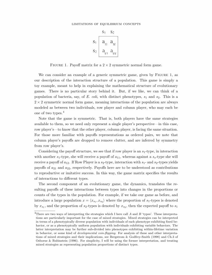
Figure 1. Payoff matrix for a 2× 2 symmetric normal form game.

We can consider an example of a generic symmetric game, given by Figure 1, as

our description of the interaction structure of a population. This game is simply a

toy example, meant to help in explaining the mathematical structure of evolutionary

games. There is no particular story behind it. But, if we like, we can think of a

population of bacteria, say, of E. coli, with distinct phenotypes, s1 and s2. This is a

2× 2 symmetric normal form game, meaning interactions of the population are always

modeled as between two individuals, row player and column player, who may each be

one of two types.4

Note that the game is symmetric. That is, both players have the same strategies

available to them, so we need only represent a single player’s perspective—in this case,

row player’s—to know that the other player, column player, is facing the same situation.

For those more familiar with payoffs representations as ordered pairs, we note that

column player’s payoffs are dropped to remove clutter, and are inferred by symmetry

from row player’s.

Considering the payoff structure, we see that if row player is an s1-type, in interaction

with another s1-type, she will receive a payoff of a11, whereas against a ss-type she will

receive a payoff of a12. If Row Player is a s2-type, interaction with s1- and s2-types yields

payoffs of a21 and a22, respectively. Payoffs here are to be understood as contributions

to reproductive or imitative success. In this way, the game matrix specifies the results

of interactions to different types.

The second component of an evolutionary game, the dynamics, translates the re-

sulting payoffs of these interactions between types into changes in the proportions or

counts of the types in the population. For example, if we take our game as before, and

introduce a large population x = 〈xs1 , xs2〉 where the proportion of s1-types is denoted

by xs1 , and the proportion of s2-types is denoted by xs2 , then the expected payoff to s1

4There are two ways of interpreting the strategies which I here call A and B ‘types’. These interpreta-tions are particularly important for the case of mixed strategies. Mixed strategies can be interpretedin terms of a phenotypically diverse population with individuals of each phenotype exhibiting fixed be-havior, or as a phenotypically uniform population with individuals exhibiting variable behaviors. Thelatter interpretation may be further sub-divided into phenotypes exhibiting within-lifetime variationin behavior, or some kind of developmental coin-flipping. For analysis of these and other interpreta-tions of mixed strategies and their implications, see Bergstrom & Godfrey-Smith (1998) and Ch.3 ofOsborne & Rubinstein (1996). For simplicity, I will be using the former interpretation, and treatingmixed strategies as representing population proportions of distinct types.

aydin mohseni

and s2 types will be given by u(s1, x) = a11xs1 + a12xs2 and u(s2, x) = a21xs1 + a22xs2 ,

respectively. These may be read as the expected reproductive success of the types,5 and

determine their representation in the population in the next generation. With the intro-

duction of a dynamics, the relative proportions of the types in the population affect the

payoffs to each strategy, and so fitness becomes dependent on the relative frequencies

of types.

The negative results in this paper hold for finite games generally. For our results, we

will use the simplest games in which they may be produced: two- and three-strategy

symmetric normal form games. For our dynamics, we consider the replicator dynamics

(RD), the “first and most important model of evolutionary game theory” (Cressman

and Tao 2014, 1081). The leading idea behind the replicator dynamics is that types

that are more fit than the population average fitness grow in relative proportion, and

types that are less fit than average shrink in proportion. This can be described by a

system of differential equations.6

xi = xi [u(i, x)− u(x, x)] , i = 1, 2, . . .

where x denotes the rate of change of the population proportion of strategy i, xi denotes

the proportion of strategy i, u(i, x) denotes the expected fitness of type i from interaction

with the population, u(x, x) denotes the population mean fitness, and x denotes the

composition of the population as a whole.

An equilibrium, then, is just a fixed or stationary point of the dynamics. In the

continuous time replicator dynamics, a state x is a fixed point of the dynamics if xi =

0 for all i. Not all equilibria are made equal. Some sets of equilibria will, either

individually or collectively, constitute plausible outcomes of a dynamics, while others

will not. As we will see, the measure of a successful equilibrium concept is in making

just such a distinction, and selecting the right subset of possible outcomes. For reasons

we will discuss, the challenge is nontrivial.

3. Capturing Evolutionary Significance

To present our central argument, we need a clear understanding of how to evaluate

the success and failure of equilibrium concepts in the context of evolutionary games.

This is typically explained in terms of “capturing evolutionary significance.” That is,

it is assumed that for an equilibrium concept to be successful it must capture all and

only the states of an evolutionary process that are probable outcomes of that process.

5In the simple case where the game determines each type’s fitness completely.6The Replicator dynamics admits a discrete time formulation—the Maynard-Smith dynamics (1982)—,which, under some conditions, yield subtly different results from their continuous time counterpart(Cressman 2003). For discussion of discrete and continuous time formulations of RD see (Schuster andSigmund 1983)

limitations of equilibrium concepts

Figure 2. Payoff matrix and phase portrait of a dynamics with a singleprobable outcome.

The notion of evolutionary significance has been used a number of times in the EGT

literature (Skyrms 2000; Huttegger and Zollman 2010, 2013). When Hutteger and

Zollman state ”Many non-ESS states are evolutionarily significant” (2010, 13), this is

the notion they are employing. But evolutionary significance has yet to be explicitly

defined—to-date, it has been an essentially informal desideratum for determining the

explanatory important of predictions derived from evolutionary models. We attempt to

provide such a definition in the context of evolutionary games, and in doing so, arrive

at a novel probabilistic account of evolutionary significance. Our definition proposes a

clear connection between the heretofore informal notion of evolutionary significance and

the formal definitions of equilibrium concepts from game theory and stability concepts

from the study of dynamical systems.

To begin, what we want to say is something to the following effect: that the significant

outcomes of an evolutionary dynamic are just those that are the probable outcomes of

that dynamic. At first pass, this yields the characterization:

Characterization 1 (Evolutionarily Significant Outcome). Given an evolutionary game

and its dynamics, an outcome is evolutionarily significant if it is a probable outcome of

that dynamics.

But this definition needs be unpacked and sharpened in turn, and we must continue

unpacking and sharpening the assumptions implicit in evolutionary significance until

we arrive at those amenable to precise formulation. The result of this process will be

to provide us with the criteria needed to evaluate the success of equilibrium concepts.

First, we unpack the notion of probable outcome.

To illustrate the concepts involved, we can proceed by use of the example of an

evolutionary game which exhibits a single probable outcome. Let the simplex in Figure

2 be the state space of a simple 3-strategy symmetric evolutionary game. Each point in

the simplex represents a possible population state—a vector x = 〈xa, xb, xc〉 specifying

the population proportions of the strategies a, b, and c. The three vertices represent the

monomorphic states where the population is composed entirely of a single strategy, so

the a-vertex corresponds to the state vector 〈1, 0, 0〉, and so on. Distance from a vertex

aydin mohseni

corresponds inversely to the population proportion of the strategy represented by the

vertex.

Given a game, the dynamics specify how the state vector changes over time, moving it

through the state space of possible population proportions. The path that a population

moves along in the state space as it evolves is called its trajectory. Which trajectory

a population takes depends on its initial conditions. We visualize the “flow” induced

on the state space by the replicator dynamics by drawing representative trajectories

where the directions of flow are designated by using arrows as in Figure 2. Diagrams

such as Simplex II in Figure 2 may be used to represent our game dynamics and are

called phase portraits. Here, dotted lines represent sets of fixed points, opaque circles

represent sinks, and empty circles represent sources.

In this game, we would clearly want to say that the state in which strategy c dominates

the population is the sole probable outcome of evolution. Our reasoning is as follows.

We begin by assuming that it is there is some positive probability that population will

start in any open interval of the state space.7 (For example, in the simplest case, this

can be a uniform distribution.) It follows from this stipulation that we must assign a

continuous probability distribution over every point in the state space with respect to

the initial conditions of the dynamic.

Next, we observe that the dynamics indicate that from most any starting point, the

population will evolve toward the all-c vertex of our simplex, where the population is

composed entirely of individuals using strategy c. We further observe that, from any

state where the proportion of strategy c is nonzero, the dynamics will converge, in the

limit of time, to the state where the population proportion of strategy c is one. Thus,

it appears that the state x∗ = 〈0, 0, 1〉 where only strategy c is present is a probable

outcome of the game.

We can further develop our concept of a probable outcome by considering what may

constitute an improbable outcome. Consider the dotted edge ab at the bottom of the

simplex: this line corresponds to the population mixtures of a and b where strategy

c is wholly absent. At all population states along this line, excepting its endpoints,

strategies a and b receive the same fitness. There is no selective pressure in either

direction since

ua = x ·A(a, a) + (1− x) ·A(a, b) = 1 = x ·A(b, a) + (1− x) ·A(b, b) = ub,

where x and (1 − x) denote the proportions of strategies a and b, respectively. Given

that the fitness of both strategies is equal, it seems that a population starting at this

edge would have no reason to leave, and so would remain here for all time.

Given a continuous distribution over initial conditions, however, the chances of ac-

tually starting on this edge are negligible, since any one-dimensional edge composes a

7To do so, we assume the Lebesgue measure on the n-dimensional volume of the state space ∆n ={〈x1, . . . , xn〉 |xi ≥ 0,

∑xi = 1}, where n ≡ |S| denotes the cardinality of the strategy set of the game.

limitations of equilibrium concepts

measure-zero subset of our two-dimensional space.8 By this reasoning, the set of states

composing ab constitute improbable initial conditions of the population, and so, are not

a probable outcome of our dynamic.

But what if our priors are not continuously distributed on the whole state space?

Imagine that we know that the population will start at one of the population states

represented by the edge ab. In this case, we may ask again: does any portion of the edge

ab compose a probable outcome of our evolutionary dynamics? Perhaps surprisingly, our

conclusion must remain that no subset of the edge is a probable outcome of evolution.

The reason for this is a “hidden mutation assumption.” That is, while it is not explicitly

represented in the replicator dynamics, we assume that there is some possibility of

invasion by mutant. Small numbers of any alternative strategy may be produced by

mutation and lead to small but persistent fluctuations in the population proportions.

Here, any small perturbations of the population state from the edge would cause the

population to head off toward the top of the state space, never to return. The inevitable

presence of mutant strategies and natural fluctuations means that an outcome cannot

be a probable one unless it is stable under small perturbations.

We now have a definition of probable outcome in terms of convergence from a signif-

icant set of initial conditions, and resistance to small perturbations.

Characterization 2 (Probable Outcome). An outcome is probable if, given a con-

tinuous probability distribution on initial conditions of the state space, a set of initial

conditions of positive measure converge to the outcome, and, upon convergence, are

stable in the face of small perturbations.

But we must also be precise about what constitutes an outcome? In order to provide

a principled and unifying formulation of what constitutes an outcome of a nonterminal

process, we must lean on the notion of limits. An outcome, then, becomes a possible

behavior of the system in the limit of time. Thus we have

Characterization 3 (Outcome). An outcome is a possible behavior of an evolutionary

game in the long run, as time goes to infinity.

But there is still something more we want to say. Outcomes should not be limited to

convex sets of states. Outcomes should include (sets of) closed orbits. For example, in

the rock paper scissors (RPS) game in Figure 3, the limit behavior of the dynamics is

a continuum of cycles around the center point of the state space, and any point on the

interior of the simplex is a part of some cycle for some initial conditions of the system.

So while no single orbit is a probable outcome, the continuum of orbits is. What we

have is that sets of closed orbits, and not only sets of states, may be outcomes of a

dynamics.

8More generally, any (n − 1)-dimensional subspace of an n-dimensional state space will be assignedmeasure zero.

aydin mohseni

Figure 3. Rock-paper-scissors game exhibiting cycles.

This allows us to capture key disequilibrium behavior such as limit cycles and strange

attractors that may constitute persistent long run outcomes of dynamics (Skyrms 1992b;

Wagner 2012). With this, we have arrived at formal conditions by which to evaluate

equilibrium concepts. We combine characterizations 2, and 3 to get:

Characterization 4 (Evolutionary Significance). A set of states or closed orbits is a

evolutionarily significant if, given a continuous probability distribution on initial condi-

tions of the state space, a set of initial conditions of positive measure converge to the

set in the limit of time, where they are stable in the face of small perturbations.9

We have characterized evolutionary significance in terms of probable outcomes under

some evolutionary dynamics, and probable outcomes as states (or closed orbits) that

induce convergence from a significant set of initial conditions, and exhibit stability under

perturbations. This is what we want, as we can mathematically formalize the concepts

of attraction and stability in the form of our stability concept, and we can then use the

stability concept to evaluate the success and failure of equilibrium concepts. For our

results, this will end up being asymptotic stability.10

Having arrived at a sharper definition of evolutionary significance for this context,

we can return to the simple evolutionary game in Figure 2 to conclude that the sin-

gle probable outcome of this evolutionary game is the monomorphic population state

x∗ = 〈0, 0, 1〉 where strategy c has come to fixation. The state x∗ is evolutionarily

significant because it commands convergence from a probabilistically significant set of

initial conditions composed of the interior of the simplex, and any population already

at x∗ is stable. There are no other evolutionarily significant (sets of) states, as any

points not on in the interior of the simplex is on its edges, and the edges of the simplex

compose a measure-zero subset of the state space, and so do no constitute probable

initial conditions.

9We should note that this allows for evolutionary significance to be relativized to known initial condi-tions that may compose strict subsets of the state space. In practice, if we have an informed probabilitydistribution over initial conditions (e.g., inferred from the biological record or determined by exper-imental controls), we can speak of probable outcomes relative to these initial conditions. It can beshown that restricting the set of initial conditions with positive probability can eliminate, but not add,to the set of evolutionarily significant outcomes of a game.

10Though as we will see, this will not quite suffice to capture (sets of) closed orbits.

limitations of equilibrium concepts

4. Stability Concepts

We have provided a sharper definition of evolutionary significance so that we can have

clarity about the connection between our intuitive notion of evolutionary significance

and mathematical precise formulations of this notion. These formulations are stability

concepts.

First, we note that a basic fact about stability concepts is that they are dynamics-

specific. Stability concepts are defined in relation to dynamics, or classes of dynamics.

For our results, we will define the stability concepts for the replicator dynamics. The

main candidate stability concepts are asymptotic stability, and Lyapunov stability.

Definition 1 (Lyapunov Stable). A stationary state is stable if points near it remain

near it.

Definition 2 (Attracting). A stationary state is attracting if nearby points tend toward

it.

Definition 3 (Asymptotically Stable). A stationary state is asymptotically stable if it

is both stable, and attracting.11

The stability concept provides criteria for evolutionary significance in relation to

the game dynamics. By being defined in terms of the dynamics, the stability concept

provides a richer, more reliable but less general notion than that which can be provided

by an equilibrium concept.12 It becomes clear then, that if the underlying dynamics is

taken seriously, the goal of the equilibrium concept should be to pick out essentially the

same (sets of) states as the stability concept.

5. Equilibrium Concepts

Equilibrium concepts were imported into evolutionary game theory from classical,

rational choice game theory. An essential insight that has motivated the adaptation of

equilibrium concepts into evolutionary game theory is that evolutionary processes can

be thought of as solving optimization problems in a way not entirely dissimilar to the

recommendations made to rational agents in classical game theory. Where strategies

maximizing individual expected utilities may deliver a group of rational agents to an

equilibrium, evolutionary dynamics driven by differentials in reproductive or imitative

success may deliver populations of non-rational, or bounded rationality, agents to stable

states.

The candidate equilibrium concepts are: Nash equilibrium (NE), strict Nash equi-

librium, evolutionary stable strategies (ESS), neutrally stable strategies (NSS), and

11For precise definitions of the stability concepts see (Cressman [2003], pp.18-19).12Note that these stability concepts also omit some of the outcomes we want to deem as evolutionarily

significant, such as cycles and strange attractors. However, for now, asymptotic stability gives us asufficient and precise characterization of significant outcomes. We will return to exceptional cases inlater sections.

aydin mohseni

Figure 4. A diagram of the interrelationship of evolutionary signifi-cance, equilibrium concepts, and stability concepts.

evolutionarily stable sets (ESSets).13 Each equilibrium concept is a refinement of the

Nash equilibrium. That is, each starts with the set of Nash equilibria of a game and

trims down the set by eliminating those equilibria it deems implausible (Huttegger et al.

2014). The exception to this is the ESSet concept. Rather than assessing individual

equilibrium states, the ESSet picks out sets of states that, when considered collectively,

exhibit equilibrium properties.

Formally, an equilibrium concept is a mapping F : Γ→ ∪G∈Γ2∆G from the set of all

games Γ to the union of the states spaces of all possible strategy profiles. That is, F

takes as arguments a game G, and the set of the possible states ∆G for that game (its

state space, as previously defined), and outputs a subset F (G,∆G) of those states. For

our applications to evolutionary games, the aim is that one of these subsets turns out

to be just the evolutionarily significant outcomes of that game.

What is crucial to observe is that, whereas stability concepts are defined in relation

to the evolutionary dynamics, equilibrium concepts are defined exclusively in relation

to the interaction structure of the strategies. That is, equilibrium concepts are defined

exclusively in terms of the game. That equilibrium concepts can be used to attempt

to infer the plausible outcomes of evolution by considering only the game matrix—and

without deferring to any specific underlying model of the evolutionary dynamics—is

essential to both their theoretical simplicity and generality, and, ultimately, to their

limitations and unreliability.

In Figure 4, the interrelationship of evolutionary significance, equilibrium concepts,

and stability concepts is visualized. In (1), our informal notion of evolutionary signif-

icance must be made mathematically precise in the form of a stability concept, which

must be defined with respect to some (class of) evolutionary dynamics. In (2), we can

now evaluate the equilibrium concept, defined at the level of the game matrix, in terms

13One may consider other equilibrium concepts from game theory, such as the subgame perfecti equi-librium, trembling hand equilibrium, sequential equilibrium, and so on. However, for various reasons,they are not typically seen as candidates for evolutionary games, and so are not considered here.

limitations of equilibrium concepts

of its agreement with the stability concept. This gives us, in (3), a way to indirectly

assess the success of a given equilibrium concept in capturing evolutionary significance

under a given class of matrices and dynamics. For us, these are finite games under the

replicator dynamics.

In this way, equilibrium concepts explain evolutionary significance in so far as they

are in agreement with the stability concept; we assess each equilibrium concept by its

success in capturing the set of states that are asymptotically stable.

We have presented a novel, and more precise formulation of evolutionary significance

that we argue captures what implicitly underpins determination of the success of equi-

librium concepts. We have formalized this definition as a stability concept—asymptotic

stability— that is defined in relation to a hypothesis as to the behavior of evolution—the

replicator dynamics. With this, we have established a framework in which we can as-

sess the viability of an equilibrium concept—in terms of its agreement with the stability

concept, and hence with our conditions for evolutionary significance.

6. Methodology of Analysis

The results gathered in this paper collectively demonstrate that even under favorable

assumptions regarding the underlying dynamics and standards of stability—replicator

dynamics and asymptotic stability—all candidate equilibrium concepts fall short. The

approach taken here, and in much of the literature, is to test the equilibrium concepts

under assumptions constituting a “best-case scenario.” The idea is that, if the equilib-

rium solution concepts fail under such assumptions, a sort of informal “upper bound” for

the domain of their reliable application has been established. For these results to carry

weight, we must justify why replicator dynamics and asymptotic stability constitute

such a best case for our equilibrium solution concepts.

Among evolutionary dynamics, the replicator dynamics are commonly regarded as the

simplest member of the class of deterministic dynamics (Sandholm 2010). Our claim is

that if an equilibrium concept fails to capture evolutionary significance for the replicator

dynamics, then it has little hope to do so for other more complicated dynamics. The

reason for this is that RD make largely the same assumptions about the population as

the ESS concept does (Apaloo et al. 2009). This should not come as a surprise, as the

RD were formulated by Taylor and Jonker (Taylor and Jonker 1978) specifically for the

purpose of providing an explicit evolutionary dynamic for the ESS concept. And as all

of our candidate equilibrium concepts are refinements of the Nash equilibrium concept,

just as ESS is, they carry largely the same assumptions as to the nature of evolutionary

populations involved. Specifically, each of the equilibrium concepts can be thought of

as implicitly assuming infinite populations, no drift, no population structure, and a

uniform environment.

aydin mohseni

To see how these assumptions make the replicator dynamics congenial to our equilib-

rium concepts, consider two somewhat more complex dynamics—the replicator-mutator

dynamics, and the Moran process. The replicator-mutator dynamics differ from RD only

in that they make mutation explicit (Bomze and Burger 1995), while the Moran process

provides a stochastic analogue to RD, allowing for the modeling of finite populations

and the concomitant effects of drift (Moran 1962). In the former dynamics, sufficiently

high mutation rates can obviate any equilibrium prediction by changing the position of

equilibria, and potentially collapsing fixed points of the dynamics (Hofbauer and Hut-

tegger 2007). In the latter, small population sizes can select even for strictly dominated

strategies (Fudenberg and Imhof 2004), defying a basic assumption of the equilibrium

concepts.14 In both cases, for the same game, parameters not represented at the level

of the game matrix—mutation rate and population size—can be changed so as to lead

to qualitatively distinct outcomes. Equilibrium concepts take as input only the payoff

matrix and state space of game, and so cannot be sensitive to parameters not reflected

in these two objects. In contrast to the replicator-mutator dynamics and Moran process,

the replicator dynamics, given any game, will output a qualitatively unique evolution-

ary process (Weibull 1997). The RD are, by design, highly congenial to our equilibrium

concepts.

Similarly, asymptotic stability is the most common stability concept used in tan-

dem with deterministic dynamics, generally, and the replicator dynamics, specifically

(Hofbauer and Sigmund 1998; Cressman 2003; Sandholm 2010). Stronger stability con-

ditions—those that pick out fewer (sets of) states as stable—will cause the equilibrium

concepts to perform worse, as the equilibrium concepts are already too weak with respect

to asymptotic stability, and pick out many states it deems as unstable. Similarly, under

the weaker assumption of Lyapunov stability it is known that the RD’s performance is

even worse (Bomze 1983, 1995). These results suggest that asymptotic stability may

provide something in the neighborhood of locally optimal stability conditions for the

replicator dynamics.

7. The Limitations of Equilibrium Concepts

We can now present an overview of the existing results on the limitations of equilib-

rium concepts in light of a unifying definition of evolutionary significance. We provide

citations of original results where appropriate. A natural place to begin our overview

and analysis is at the Nash equilibrium (NE) concept. This is because, in their logical

structure, all of the equilibrium concepts we will be considering here are refinements of

the NE concept. That is, each equilibrium concept can be thought of as beginning with

the full set of Nash equilibria, and proceeding to eliminate those equilibria it deems are

14That is, a strictly dominated strategy can never be a best response, and so cannot be a part of aNash equilibrium.

limitations of equilibrium concepts

Figure 5. The flow of the implication relations between equilibriumconcepts and stability concepts.15

unviable. The exception to this narrowing is the ESSet concept as it also expands the

range of equilibrium states to allow for sets of states that are collectively (though not

necessarily individually) asymptotically stable.

Each of these Nash refinements—the strict NE, ESS, NSS, and ESSet—will be shown

to be, in one or more ways, too weak, in that they pick out (sets of) states that are not

evolutionarily significant. Some equilibrium concepts will also be shown to be too strong

in that they fail to pick out evolutionarily significant (sets of) states. Additionally, we

will find that all equilibrium concepts share a way in which they are uniformly too

strong: they all fail to capture intuitively significant outcomes, such as limit cycles and

strange attractors, that are not expressible in terms of sets of states.

7.1. Limits of the Nash Equilibrium and Strict Nash Equilibrium. The Nash

refinements project is bounded by the following two observations: the Nash equilibrium

is far too weak, and the strict Nash equilibrium far too strong. The former includes

in its predictions states which are neither stable nor attracting, and the latter omits

states which are both. Given these bounds, one might hope that an equilibrium concept

intermediate in strength may pick out all and only evolutionary significant outcomes.

This turns out not to be so.

The Nash equilibrium is the fundamental equilibrium concept of classical, rational

choice game theory. A state is a NE in which no individual stands to gain by unilaterally

switching her strategy—i.e., by switching her strategy when all the strategies of all the

other players remain fixed. For a population in such a state, no individual has positive

incentive to deviate, and so it will be a fixed point. In other words, if there are no

perturbations, a population starting at that state will remain at that state. Formally,

we define the NE as follows:16

Definition 4 (Nash Equilibrium). A state x ∈ X is a Nash equilibrium if, for all y ∈ ∆

where y 6= x, u(x, x) ≥ u(y, x).

16For simplicity, we provide definitions for the case of symmetric pairwise interactions. For the mathe-matically inclined, extensions to more general games should be clear.

aydin mohseni

Figure 6. The all-a state 〈1, 0〉 is a Nash equilibrium of the game, butis unstable under the replicator dynamics.

where u(x, x) can be thought of as the fitness of a incumbent population x in inter-

acting with itself, and u(y, x) as the fitness of an alternative (mixture of) type(s) y in

interacting with a population composed of the incumbents.

What is important to note about the Nash equilibrium concept is that all NE are

fixed points under RD. The converse, however, is not true. Not all fixed points are

NE. This is because, under RD, every unused strategy remains unused, and every pure

strategy corresponds to a state of the population in which all but one strategy is unused.

Hence, that single strategy will be the only strategy present for all future times as its

population proportion will remain constantly at one. Thus, every pure strategy is a

fixed point of the dynamics. However, all interior fixed points are indeed NE (Weibull

1997).

To demonstrate that the Nash equilibrium provides conditions too weak for evolu-

tionary significance, we need only observe how fixed points that are neither stable nor

attracting (these are known as sources) may be NE. Consider the simple symmetric

2× 2 game in Figure 6. Both the monomorphic populations—those composed entirely

of strategies a or b, corresponding to the state vectors 〈1, 0〉 and 〈0, 1〉—are Nash equi-

libria. In each monomorphic state, no single individual stands to gain by unilaterally

changing her strategy. Yet, the monomorphic population state 〈1, 0〉 composed of only

a-types is not stable: it is a source, and the phase portrait reveals that the slightest

perturbation will send the population straight off toward strategy b corresponding to

the population state 〈0, 1〉.Sources represent an extreme case of instability. No source can be asymptotically

stable, and so, by our criteria, we can conclude that no source can be evolutionarily

significant. Yet, NE may well be sources. This fact suffices to demonstrate that the

Nash equilibrium is too weak a concept. This line of thinking provides the motivation

for the following refinements of the NE concept that strengthen its requirements with

the aim of narrowing in on the subset of viable equilibria by eliminating implausible

fixed points.

We may strengthen the Nash equilibrium concept to the strict Nash equilibrium. The

strict NE has the virtue of eliminating all the unstable states captured by the plain NE.

Sources cannot be strict NE. However, the strict NE is clearly too strong, and eliminates

limitations of equilibrium concepts

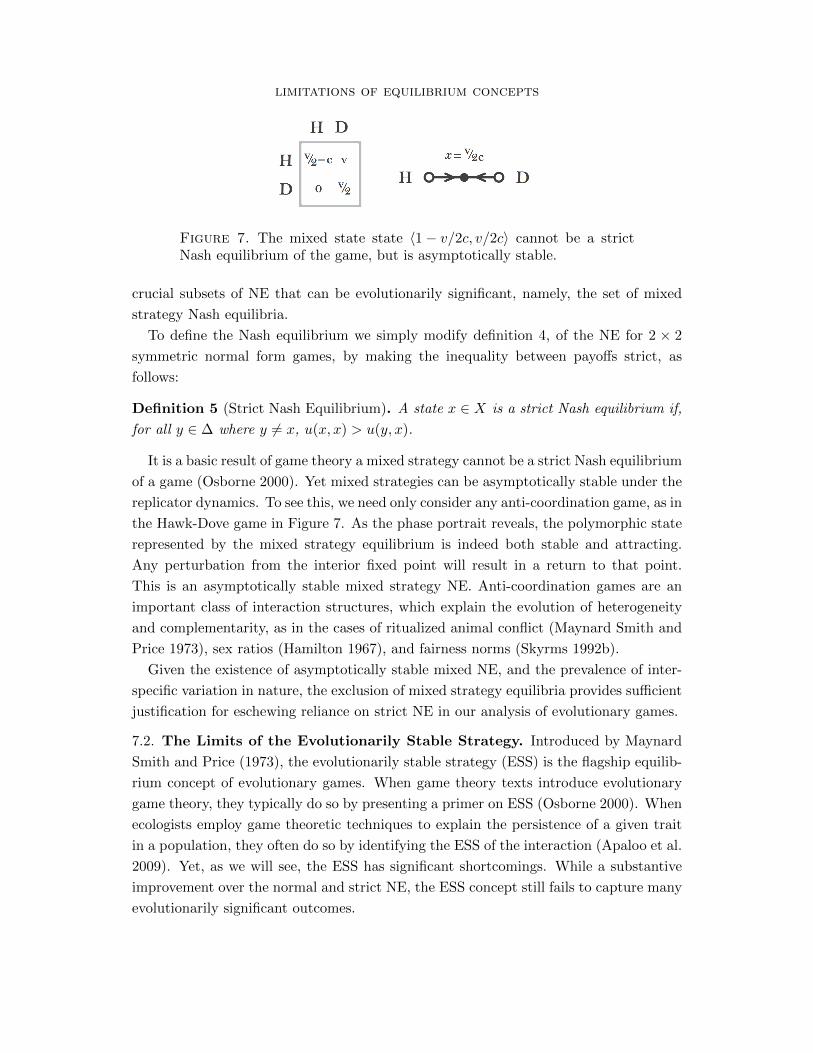
Figure 7. The mixed state state 〈1− v/2c, v/2c〉 cannot be a strictNash equilibrium of the game, but is asymptotically stable.

crucial subsets of NE that can be evolutionarily significant, namely, the set of mixed

strategy Nash equilibria.

To define the Nash equilibrium we simply modify definition 4, of the NE for 2 × 2

symmetric normal form games, by making the inequality between payoffs strict, as

follows:

Definition 5 (Strict Nash Equilibrium). A state x ∈ X is a strict Nash equilibrium if,

for all y ∈ ∆ where y 6= x, u(x, x) > u(y, x).

It is a basic result of game theory a mixed strategy cannot be a strict Nash equilibrium

of a game (Osborne 2000). Yet mixed strategies can be asymptotically stable under the

replicator dynamics. To see this, we need only consider any anti-coordination game, as in

the Hawk-Dove game in Figure 7. As the phase portrait reveals, the polymorphic state

represented by the mixed strategy equilibrium is indeed both stable and attracting.

Any perturbation from the interior fixed point will result in a return to that point.

This is an asymptotically stable mixed strategy NE. Anti-coordination games are an

important class of interaction structures, which explain the evolution of heterogeneity

and complementarity, as in the cases of ritualized animal conflict (Maynard Smith and

Price 1973), sex ratios (Hamilton 1967), and fairness norms (Skyrms 1992b).

Given the existence of asymptotically stable mixed NE, and the prevalence of inter-

specific variation in nature, the exclusion of mixed strategy equilibria provides sufficient

justification for eschewing reliance on strict NE in our analysis of evolutionary games.

7.2. The Limits of the Evolutionarily Stable Strategy. Introduced by Maynard

Smith and Price (1973), the evolutionarily stable strategy (ESS) is the flagship equilib-

rium concept of evolutionary games. When game theory texts introduce evolutionary

game theory, they typically do so by presenting a primer on ESS (Osborne 2000). When

ecologists employ game theoretic techniques to explain the persistence of a given trait

in a population, they often do so by identifying the ESS of the interaction (Apaloo et al.

2009). Yet, as we will see, the ESS has significant shortcomings. While a substantive

improvement over the normal and strict NE, the ESS concept still fails to capture many

evolutionarily significant outcomes.

aydin mohseni

Figure 8. A globally attracting non-ESS.

In a symmetric normal form game, an ESS is a strategy with the following property:

a population in which nearly all individuals play this strategy is resistant to invasions

by small groups of mutants playing any alternative strategy. Formally,

Definition 6 (Evolutionarily Stable Strategy). A state x is evolutionarily stable if, for

all y ∈ ∆ where y 6= x, there exists an ε(y) > 0 such that (1 − ε) · (x, x) + ε · (x, y) >

(1− ε) · (y, x) + ε · (y, y) for 0 < ε < ε(y).

In an ESS, the expected payoffs to the incumbent strategy x is strictly greater than

that of any alternate strategy y, used by a sufficiently small proportion ε of mutants in

the population. Equivalently, in a way that makes its relation to the NE clear, the ESS

may be formulated in terms of the combination of two conditions:

Definition 7 (Evolutionarily Stable Strategy). A state x is evolutionarily stable if, for

all y ∈ ∆ where y 6= x,

(1) u(x, x) ≥ u(y, x), and

(2) if u(x, x) = u(y, x), then u(x, y) > u(y, y).

The first condition states that the incumbent strategy x composes a (weak) NE with

itself, and the second condition says that if there is a mutant y who fairs as well against

x as it does against itself, then x must do better against that mutant that it does against

itself. That is, any mutant strategy must not be able to invade, and moreover must also

be driven to extinction.

When compared to the strict NE, the ESS represents a clear move in the right direc-

tion. As with strict NE, with ESS we retain the guarantee of asymptotic stability, but

unlike the strict NE, the ESS doesn’t automatically disqualify mixed strategy equilibria.

In one direction, we have that if a state is an ESS, then it is indeed asymptotically

stable. In the other direction, however, the implication does not hold. There are

attracting states, and attracting sets of states that are not ESS. There are stable states

and stable sets of states that are not ESS. And there are AS states, and collectively AS

sets of states that are not ESS (Bomze 1983, 1995).

We consider examples of non-ES states and sets of states, as these are both attracting

and stable. The reason that a stable attractor may not be an ESS is that the dynamics

limitations of equilibrium concepts

Figure 9. The set of states in {〈a, b, c〉 | a = b, c ∈ [0, 1]} are collectively,but not individually, asymptotically stable.

may spiral in elliptically towards the attractor. This cannot be covered by the notion

of ESS due to the linearity inherent in its definition. To see this, we consider the

game in Figure 8, where we have a global attractor that is not an ESS. Here, the point

x = 〈1/3, 1/3, 1/3〉 is no ESS, but globally attracting. It is readily observed that any

interior state will converge to x, and we can confirm that x is not an ESS by working

through Definition 7 of ESS. First we observe that if one individual uses x then the

other player gets an expected payoff of 1 no matter what strategy they use. That is, for

any alternate strategy y, u(x, x) = 1 = u(y, x). So condition (1) of ESS is satisfied, and

no strategy does better against x than it does against itself. But this payoff tie means

that we need to check the condition (2), which is indeed not satisfied.

To see this, consider a perturbed state such as y = 〈3/8, 1/4, 3/8〉. Here, we get

u(x, y) ≈ 1.031 > 0.96 ≈ u(y, y) and so the mutant strategy y fares better against itself

than x does against it. But the mutant’s advantage is temporary as y is unstable and

gives way to the invasion of another mutant strain, which gives way to another, and so

on, with an orbit which spirals in towards x. A similar example of an attractor with

a large basin of attraction is provided by Zeeman’s 1981 counterexample depicted in

Figure ??.

What these examples show is that, from the point of view of RD, an attractor is a

more general notion than an ESS, and better characterization of resistance to mutation.

Moreover, we have from (Zeeman 1981) that if an ESS lies in the interior of the state

space, then its basin of attraction is the whole interior, and so it is the only attractor.

But if an attractor is in the interior of the states space, it may have a smaller basin of

attraction, and the game may still admit other attractors on the boundary of the state

space (see Figure ??).

A defining limitation of the ESS concept is that it captures only single population

states, and so cannot capture non-singleton sets of states, whatever their basins of at-

traction or stability properties; sets of states that are collectively asymptotically stable

are beyond its reach. Consider the evolutionary game and dynamics in Figure 9. Ex-

amining the phase portrait, it is clear that interior trajectories will converge to the set

E = {〈a, b, c〉 | a = b, c ∈ [0, 1]}. But no member of E is an ESS. This is because every

aydin mohseni

distinct strategy in this set is in a payoff tie against any other, and so the second con-

dition of the ESS, that of strict inequality, will not be satisfied. Yet, when considered

collectively, this set is both globally attracting and stable—we will see that it is an

ESSet.

Why should we worry about sets of states qua sets? In normal form games, sets of

fixed points tend not to be robust under small perturbations in the payoff structure of

the game. Sets containing continua of equilibria can often be made to collapse to a single

state. In extensive form games, however, this is not so. It is a well-known property of

extensive form games with nontrivial structure that they produce non-singleton Nash

sets (Cressman 2003). Importantly, it has been shown that in many extensive form

games these sets are indeed robust under perturbations of payoffs (Huttegger 2010).

Moreover, as in Figure 9, no single state in the attracting set is evolutionarily signifi-

cant, since the set of initial conditions that will converge to any point in E is a measure

zero set. It is only the set as a whole that commands convergence from a non-measure

zero set of initial conditions, and so only the set as a whole qualifies as evolutionarily sig-

nificant. Sets of states that are significant only as sets should be expected, particularly

in extensive form games, and should be accounted for.

In short, the conditions provided by the ESS are clearly too strong in that they fail

to capture (globally) attracting states, as well as some asymptotically stable states, and

all collectively asymptotically stable sets of states.17

7.3. The Limits of the Neutrally Stable Strategy. The neutrally stable strategy

(NSS) relaxes the ESS concept to weak inequality so as to include more evolutionarily

significant outcomes. Particularly, it redeems some, though not all, of the Lyapunov

stable states excluded by the ESS. An advantage of the NSS over the ESS is that it can

account for members of significant Nash components, as well as portions of some limit

cycles. In the latter case, the hubs of cycles can be NSS (e.g., in the RPS game), while

the orbits themselves will go uncaptured. A basic property of an NSS under RD is that

it is Lyapunov stable (Weibull 1997). The converse is not generally true, and we will

see that there can be Lyapunov stable states that are not NSS. A NSS is not necessarily

attracting, and so it is not necessarily asymptotically stable. There are evolutionarily

insignificant NSS, as demonstrated by n > 1-player degenerate games A = [0], where

every point in the state space is an NSS with a measure-zero basin of attraction. The

NSS captures some evolutionarily significant states neglected by the ESS at the expense

of including other insignificant states.

Intuitively, at an NSS, mutant strategies will not be able to invade, but neither will

they be driven out. Formally, the NSS is a weakening of the ESS to weak inequality in

condition (2).

17For an analysis on asymptotically stable sets see (D’Aniello and Steele 2006).

limitations of equilibrium concepts

Figure 10. The set of states {〈a, b, c〉 | a = b > 0} are Lyapunov stable,but not NSS.

Definition 8 (Neutrally Stable Strategy). A state x is neutrally stable if, for all y ∈ ∆

where y 6= x,

(1) u(x, x) ≥ u(y, x), and

(2) if u(x, x) = u(y, x), then u(x, y) ≥ u(y, y).

To see what significant states the NSS captures that the ESS does not, we revisit the

game in Figure 9 with an asymptotically stable set, none of the members of which are

ESS. Because of the relaxing of condition (2) to non-strict inequality in the NSS, all of

the states that are eliminated by the ESS remain; the NSS captures each of the states

belonging to the set. Again, however, NSS is defined for individual states and cannot

account for the set qua set. This is unfortunate, since it is the set that is asymptotically

stable, whereas any one of its members is only Lyapunov stable.

Let us consider an example demonstrating that the converse to the essential property

of NSS does not hold—that not all Lyapunov stable states are NSS. Consider the game

and state space in Figure 10. Here, all population states x = 〈a, b, c〉 with a = b > 0

are Lyapunov stable, but only those with 1/3 ≤ a ≤ 1/2 are also NSS. Define the set

of Laypunov stable states as ∆LS = {〈a, b, c〉 | a = b > 0, c ∈ [0, 1]} and the set of NSS

∆NS = {〈a, b, c〉 | a = b > 0, a ∈ [1/3, 1/2], c ∈ [0, 1]}. Let x belong to ∆LS , say x =

〈1/4, 1/4, 1/2〉. Then u(x, x) = 3/4, and x is a NE with itself, however, it is not the case

that u(x, y) ≥ u(y, y) for all y. Consider y = 〈1, 0, 0〉, then u(y, y) = 1 > 3/4 = u(x, y).

Thus x is Lyapunov stable but no NSS.18

7.4. The Limits of the Evolutionarily Stable Set. The Evolutionarily stable set

(ESSets) was introduced by Bernard Thomas in (1985), and is the set-valued gener-

alization of the ESS. In many senses, ESSets represents the best option on the table.

The ESSet contains the ESS as a special case—the singleton ESSet—and so it captures

all of the evolutionarily significant outcomes that the ESS does. On top of this, all

non-singleton ESSets are also asymptotically stable, and so it captures evolutionarily

significant outcomes excluded by the ESS. An ESSet can be a global attractor in a

18Such an example was first put forward by Bomze and Weibull (1995).

aydin mohseni

broader range of cases than the ESS. Specifically, if an ESSet set contains an interior

NE, then it is globally asymptotically stable (Cressman 2003). Moreover, by construc-

tion, the ESSet fares no worse than the ESS in capturing evolutionarily insignificant

outcomes.

Definition 9 (Evolutionarily Stable Set). A closed non-empty set of strategies E is an

ESSet if and only if for each x ∈ E there exists a neighborhood B around x such that,

for all y ∈ B,

(1) If y ∈ S, then u(x, y) ≥ u(y, y), and

(2) If y /∈ S, then u(x, y) > u(y, y).

All members of an ESSet are NSS (Weibull 1997), though there are NSS that will not

belong to ESSets (Bomze 1983). From this it follows directly that there are Lyapunov

stable states that are not in ESSets. But there are also non-NSS Lyapunov stable states

that do not belong to an ESSet. Unfortunately, many of the asymptotically stable states

that are not ESS are also not ESSets.

Now, we can account for the central outcome of the games like that in Figure 10.

Recall that the set E = {〈a, b, c〉 | a = b, c ∈ [0, 1]} could not be captured by the ESS,

and was only captured by the NSS in terms of its members, which are not themselves

individually asymptotically stable. But E is an ESSet. To see this, let x ∈ E and y /∈ E.

So x and y are of the form 〈a, b, c〉 and where a = b and a 6= b respectively. By looking

at the game matrix, we see that by fixing the value of c, the game reduces to the upper

left 2 × 2 subgame where the only symmetric Nash equilibrium is where a = b. Thus

for any such y /∈ E, there is an x ∈ E such that u(x, y) > u(y, y) as required by (1). On

the other hand, if y ∈ S, by simple algebra it can be shown that u(x, y) = u(y, y).

The games in Figures 8, ??—the globally attracting non-ES state, and Zeeman’s 1981

counterexample—both also work as counterexamples for the ESSet. This follows from

the fact that they are both singleton sets of equilibria which are not ESS. Nothing in

the ESSet concept is added that can deal with them, and the same arguments as those

provided in the case of ESS carry through. Thus we still have asymptotically stable

states that are not ESSets.

Moreover, we can also find non-singleton sets which are evolutionarily significant but

not ESSets. In Figure 11 we see an of attracting set of NSS that does not belong to

an ESSet. To see how this is so, consider the set E = {〈a, b, 0〉 | b ≥ 1/2}. This is

not an ESSet, because of the boundary point x = 〈1/2, 1/2, 0〉. This can be observed

in how the state y = 〈1/2− ε, 1/2− ε, 2ε〉 fares. We find that the payoff to x against

y is u(x, y) = −ε, while the payoff to y against itself is u(y, y) = −ε/2 − ε2. For

sufficiently small values of ε we get that u(y, y) > u(x, y) violating condition (2), and

making it so that E is no ESSet. Because a single boundary point of the set is not

attracting, the set is as a whole technically not attracting. Yet we can anticipate that

all interior trajectories will end up at the set of stable states comprising E. The set

limitations of equilibrium concepts

Figure 11. The set of states in E = {〈a, b, 0〉 | b > 1/2} are all NSS,but do not belong to any ESSet.

E then constitutes an evolutionarily significant outcome by our definition, but is not

captured by the ESSet concept.19

8. Discussion

In sum, we have seen that every equilibrium concept comes up short (cf. Table 1).

The Nash equilibrium concept is far too weak. NE captures all interior fixed points,

but these include unstable states (Figure 6). Its natural modification, the strict Nash

equilibrium, is far too strong. Strict NE eliminates the unstable states captured by

the NE, but fails to capture any AS state that happens to be polymorphic (Figure 7).

The flagship ESS concept is also too strong. While the ESS captures many of the AS

polymorphic states excluded in the strict NE, it fails to collectively AS sets (Figure 9),

or AS states where the dynamic flows elliptically towards the attractor (Figure 8). The

NSS is more inclusive than the ESS, but still fails to capture some stable states (Figure

10), in addition to set-valued outcomes. The most sophisticated equilibrium concept,

the ESSet, does indeed capture many sets of collectively asymptotically stable states,

but fails to captures still others (Figure 11), and falls prey to the elliptically attracting

AS state (Figure 8) just as with the ESS.

Over and above these shortcomings, there is also a distinct in-principle argument

that these Nash refinements are all too strong. The argument is as follows. Equilibrium

concepts are formulated exclusively in terms of states or sets of states. But there

exist outcomes, such as cycles (Figure 3), which cannot be effectively expressed in such

terms. While not asymptotically stable, these are dependable regularities that can

command convergence from a significant set of initial conditions of a system, hence we

are compelled to say that they constitute evolutionarily significant outcomes. Thus,

such cycles and attractors constitute evolutionarily significant outcomes not predicted

by the equilibrium concepts. On this count equilibrium concepts are formulated in the

wrong way to begin with. This problem has no hope of being resolved by strengthening

19Apaloo et al. (2009, 510) describe this in terms of the ESSet lacking a ‘stable convergence’ property.

aydin mohseni

Equilibriumconcepts

Includes non-ES outcomes Excludes ES outcomes

Unstablestates

Non-attractingstates

Sets ofstates (quasets)

Asymptoti-cally stablestates

Limitcycles

Nashequilibrium

Yes(fig.6)

Yes(fig.6)

Yes(fig.9)

No Yes(fig.3)

Strict Nashequilibrium

No No Yes(fig.9)

Yes(fig.7,8,??)

Yes(fig.3)

Evolutionarilystable strategy

No No Yes(fig.9)

Yes(fig.8,??)

Yes(fig.3)

Neutrallystable strategy

No Yes(fig.6,10)

Yes(fig.9)

Yes(fig.8,??)

Yes(fig.3)

Evolutionarilystable set

No No No Yes(fig.8,??)

Yes(fig.3)

Table 1. Limitations of the equilibrium concepts in capturing all andonly evolutionarily significant (ES) outcomes of the replicator dynamics.

or weakening the Nash concept in just the right way. Any solution would necessarily

involve reformulating an equilibrium concept in quite different terms. How to go about

this appears to us an open question.

The challenge here is that the behavior given by limit cycles and strange attractors is

best-described in qualitatively different terms than the point-valued predictions of the

Nash refinements. Limit cycles are best described by procuring the equations that detail

their orbits (Cressman 2003), while describing the behavior of strange attractors, or even

inferring their existence, can demand the use of numerical methods (Skyrms 1992a,b).

Given this, we should not expect equilibrium concepts to provide such predictions.20

We should, however, take the presence of such evolutionarily significant disequilibrium

behavior as one more reason to avoid exclusive reliance on equilibrium concepts, and to

engage in practice of examining nontrivial dynamics on a game-by-game basis.

9. Conclusion

Our analysis of the negative results circumscribing the limitations of equilibrium con-

cepts leaves us in an interesting place. We provided a novel formulation of evolutionary

significance which makes explicits the interrelationship between evolutionary signifi-

cance, stability concepts, and equilibrium concepts. In assessing equilibrium concepts,

20We note that one promising possibility as to a more general stability concepts may lie in the notionof orbital stability.

limitations of equilibrium concepts

we have shown how stability concepts attempt to stand in for evolutionary significance,

so that a determination of the agreement between the predictions of an equilibrium con-

cept and a stability concept is a proxy for the determination of the agreement between

the equilibrium concept and evolutionary significance. This has the further virtue of

enabling the comparison of predictions between different dynamics.

In addition, we distinguish two distinct arguments against the exclusive use of equi-

librium concepts. The first is consists in the demonstration that, even under favorable

assumptions, each equilibrium concept is either too strong or too weak. The second

is an in-principle argument that observes that there are evolutionarily significant out-

comes, such as limit cycles, which cannot be effectively formulated in terms of states or

sets of states, and so cannot be predicted by equilibrium concepts.

We have not demonstrated that an equilibrium concept must fail in capturing all and

only evolutionarily significant outcomes, but we have provided arguments that we should

not expect a member of the family of Nash refinements can do the job. Our moral is

that extant equilibrium concepts on their own are typically going to be unreliable tools

for the analysis of dynamical processes, and that a more complicated, but also more

interesting picture emerges from explicit investigation of the underlying dynamics.

References

Apaloo, J., J. S. Brown, and T. L. Vincent (2009). Evolutionary game theory: ESS, convergence

stability, and NIS. Evolutionary Ecology Research 11 (4), 489–515.

Bergstrom, C. T. and P. Godfrey-Smith (1998). On the Evolution of Behavioral Heterogeneity in

Individuals and Populations. Biology and Philosophy 13, 205–231.

Binmore, K. (2005). Economic man - Or straw man?

Binmore, K. (2007). Does game theory work? The bargaining challenge, Volume 11.

Bomze, I. M. (1983). Lotka-Volterra equation and replicator dynamics: A two-dimensional classification.

Biological Cybernetics 48 (3), 201–211.

Bomze, I. M. (1995, apr). Lotka-Volterra equation and replicator dynamics: new issues in classification.

Biological Cybernetics 72 (5), 447–453.

Bomze, I. M. and R. Burger (1995). Stability by mutation in evolutionary games. Games and Economic

Behavior 11 (2), 146–172.

Bomze, I. M. and J. W. Weibull (1995). Does neutral stability imply lyapunov stability? Games and

Economic Behavior 11 (2), 173–192.

Cressman, R. (2003). Evolutionary Dynamics and Extensive Form Games. MIT Press.

Cressman, R. and Y. Tao (2014). The replicator equation and other game dynamics. Proceedings of the

National Academy of Sciences 111 (Supplement 3), 10810–10817.

D’Aniello, E. and T. H. Steele (2006). Asymptotically stable sets and the stability of ω-limit sets.

Journal of Mathematical Analysis and Applications 321 (2), 867–879.

Fudenberg, D. and L. Imhof (2004). Stochastic Evolution as a Generalized Moran Process. Unpublished

. . . , 1–26.

Hamilton, W. D. (1967). Extraordinary Sex Ratios. Science 156 (3774), 477–488.

aydin mohseni

Hofbauer, J. and S. M. Huttegger (2007). Selection-mutation dynamics of signaling games with two

signals. Language (949), 0–3.

Hofbauer, J. and K. Sigmund (1998). Evolutionary Games and Population Dynamics.

Holt, C. A. and A. E. Roth (2004). The Nash equilibrium: A perspective. Proceedings of the National

Academy of Sciences 101 (12), 3999–4002.

Huttegger, S. (2010). Generic properties of evolutionary games and adaptationism. The Journal of

Philosophy 107 (2), 80–102.

Huttegger, S., B. Skyrms, P. Tarres, and E. Wagner (2014). Some dynamics of signaling games. Pro-

ceedings of the National Academy of Sciences 111 (Supplement 3), 10873–10880.

Huttegger, S. M. and K. J. Zollman (2010). The Limits of ESS Methodology. In Evolution and

Rationality: Decisions, Co-operation and Strategic Behaviour, pp. 67–83.

Huttegger, S. M. and K. J. Zollman (2013). Methodology in biological game theory. British Journal

for the Philosophy of Science 64 (3), 637–658.

Maynard Smith, J. and G. R. Price (1973). The logic of animal conflict. Nature 246 (5427), 15–18.

Moran, P. A. (1962). The Statistical Processes of Evolutionary Theory. Clarendon Press, Oxford.

Muthoo, A., M. J. Osborne, and A. Rubinstein (1996). A Course in Game Theory. Economica.

Osborne, M. J. (2000). An Introduction to Game Theory.

Samuelson, L. (2005). Economic Theory and Experimental Economics. Journal of Economic Litera-

ture 43 (1), 65–107.

Sandholm, W. H. (2010). Population Games and Evolutionary Dynamics. The Mit Press.

Schuster, P. and K. Sigmund (1983). Replicator dynamics. Journal of Theoretical Biology 100 (3),

533–538.

Skyrms, B. (1992a). Chaos and the Explanatory Significance of Equilibrium. Proceedings of the Biennial

Meeting of the Philosophy of Science Association, 374–394.

Skyrms, B. (1992b). Chaos in game dynamics. Journal of Logic, Language and Information 1 (2),

111–130.

Skyrms, B. (2000). Stability and Explanatory Significance of Some Simple Evolutionary Models. Phi-

losophy of Science 67 (1), 94–113.

Taylor, P. D. and L. B. Jonker (1978). Evolutionarily stable strategies and game dynamics. Mathematical

Biosciences 40 (1-2), 145–156.

Thomas, B. (1985). On evolutionarily stable sets. Journal of Mathematical Biology 22 (1), 105–115.

Wagner, E. O. (2012). Deterministic chaos and the evolution of meaning. British Journal for the

Philosophy of Science 63 (3), 547–575.

Weibull, J. W. (1997). Evolutionary Game Theory. Evolutionary Game Theory. MIT Press.

Zeeman, E. C. (1981). Dynamics of the evolution of animal conflicts. Journal of Theoretical Biol-

ogy 89 (2), 249–270.

UC Irvine, Irvine, CA 92697, USA

E-mail address: amohseni@uci.edu