The Link between Default and Recovery Rates:Implications for Credit Risk Models and Procyclicality

Edward I. Altman*, Brooks Brady**, Andrea Resti*** and Andrea Sironi****

April 2002

AbstractThis paper analyzes the impact of various assumptions about the association between aggregate defaultprobabilities and the loss given default on bank loans and corporate bonds, and seeks to empiricallyexplain this critical relationship. Moreover, it simulates the effects on mandatory capital requirements likethose proposed in 2001 by the Basel Committee on Banking Supervision. We present the analysis andresults in four distinct sections. The first section examines the literature of the last three decades of thevarious structural-form, closed-form and other credit risk and portfolio credit value-at-risk (VaR) modelsand the way they explicitly or implicitly treat the recovery rate variable. Section 2 presents simulationresults under three different recovery rate scenarios and examines the impact of these scenarios on theresulting risk measures: our results show a significant increase in both expected and unexpected losseswhen recovery rates are stochastic and negatively correlated with default probabilities. In Section 3, weempirically examine the recovery rates on corporate bond defaults, over the period 1982-2000. Weattempt to explain recovery rates by specifying a rather straightforward statistical least squares regressionmodel. The central thesis is that aggregate recovery rates are basically a function of supply and demandfor the securities. Our econometric univariate and multivariate time series models explain a significantportion of the variance in bond recovery rates aggregated across all seniority and collateral levels. Finally,in Section 4 we analyze how the link between default probability and recovery risk would affect theprocyclicality effects of the New Basel Capital Accord, due to be released in 2002. We see that, if banksuse their own estimates of LGD (as in the “advanced” IRB approach), an increase in the sensitivity ofbanks’ LGD due to the variation in PD over economic cycles is likely to follow. Our results haveimportant implications for just about all portfolio credit risk models, for markets which depend onrecovery rates as a key variable (e.g., securitizations, credit derivatives, etc.), for the current debate on therevised BIS guidelines for capital requirements on bank credit assets, and for investors in corporate bondsof all credit qualities.

Keywords: credit rating, capital requirements, credit risk, recovery rate, default, procyclicality

JEL Classification Numbers: G15, G21, G28

This paper is a synthesis and analysis from the Report prepared for the International Swaps and Derivatives’ DealersAssociation. The authors wish to thank ISDA for their financial and intellectual support.*Max L. Heine Professor of Finance and Vice Director of the NYU Salomon Center, Stern School of Business, NewYork, U.S.A.** Associate Director, Standard & Poor’s Risk Solutions. Mr. Brady was a Ph.D. student at Stern when this workwas completed.*** Associate Professor of Finance, Department of Mathematics and Statistics, Bergamo University, Italy.**** Associate Professor of Financial Markets and Institutions and Director of the Research Division of SDABusiness School, Bocconi University, Milan, ItalyThe authors wish to thank Richard Herring, Hiroshi Nakaso and the other participants to the BIS conference (March6, 2002) on “Changes in risk through time: measurement and policy options” for their useful comments. The paperalso profited by the comments from participants in the CEMFI (Madrid, Spain) Workshop on April 2, 2002,especially Rafael Repullo, Enrique Sentana, and Jose Campa.

* 2 *

Introduction

Credit risk affects virtually every financial contract. Therefore the measurement, pricing

and management of credit risk has received much attention from financial economists, bank

supervisors and regulators, and from financial market practitioners. Following the recent

attempts of the Basel Committee on Banking Supervision (1999, 2001a) to reform the capital

adequacy framework by introducing risk-sensitive capital requirements, significant additional

attention has been devoted to the subject of credit risk measurement by the international

regulatory, academic and banking communities.

This paper analyzes the impact of various assumptions on which most credit risk

measurement models are presently based: namely, it analyses the association between aggregate

default probabilities and the loss given default on bank loans and corporate bonds, and seeks to

empirically explain this critical relationship. Moreover, it simulates the effects of this

relationship on credit VaR models, as well as on the procyclicality effects of the new capital

requirements proposed in 2001 by the Basel Committee. Before we proceed with empirical and

simulated results, however, the following section is dedicated to a brief review of the theoretical

literature on credit risk modeling of the last three decades.

1. The Relationship Between Default Rates and Recovery Rates in Credit Risk Modeling: a

Review of the Theoretical and Empirical Literature

Credit risk models can be divided into two main categories: (a) credit pricing models, and

(b) portfolio credit value-at-risk (VaR) models. Credit pricing models can in turn be divided into

three main approaches: (i) “first generation” structural-form models, (ii) “second generation”

structural-form models, and (iii) reduced-form models. These three different approaches,

together with their basic assumptions, advantages, drawbacks and empirical performance, are

briefly outlined in the following paragraphs. Credit VaR models are then examined. Finally, the

more recent studies explicitly modeling and empirically investigating the relationship between

the probability of default (PD) and recovery rates (RR) are briefly analyzed.

1.1. First generation structural-form models: the Merton approach

The first category of credit risk models are the ones based on the original framework

developed by Merton (1974), using the principles of option pricing (Black and Scholes, 1973). In

such a framework, the default process of a company is driven by the value of the company’s

* 3 *

assets and the risk of a firm’s default is explicitly linked to the variability in the firm’s asset

value. The basic intuition behind this model is relatively simple: default occurs when the value

of a firm’s assets (the market value of the firm) is lower than that of its liabilities. The payment

to the debtholders at the maturity of the debt is therefore the smaller of two quantities: the face

value of the debt or the market value of the firm’s assets. Assuming that the company’s debt is

entirely represented by a zero-coupon bond, if the value of the firm at maturity is greater than the

face value of the bond, then the bondholder gets back the face value of the bond. However, if the

value of the firm is less than the face value of the bond, the equityholders get nothing and the

bondholder gets back the market value of the firm. The payoff at maturity to the bondholder is

therefore equivalent to the face value of the bond minus a put option on the value of the firm,

with a strike price equal to the face value of the bond and a maturity equal to that of the bond.

Following this basic intuition, Merton derived an explicit formula for default risky bonds which

can be used both to estimate the PD of a firm and to estimate the yield differential between a

risky bond and a default-free bond 1.

Under these models all the relevant credit risk elements, including default and recovery at

default, are a function of the structural characteristics of the firm: asset volatility (business risk)

and leverage (financial risk). The RR, although not treated explicitly in these models, is therefore

an endogenous variable, as the creditors’ payoff is a function of the residual value of the

defaulted company’s assets. More precisely, under Merton’s theoretical framework, PD and RR

are inversely related. If, for example, the firm’s value increases, then its PD tends to decrease

while the expected RR at default increases (ceteris paribus). On the other side, if the firm’s debt

increases, its PD increases while the expected RR at default decreases. Finally, if the firm’s asset

volatility increases, its PD increases while the expected RR at default decreases2.

1 In addition to Merton (1974), first generation structural-form models include Black and Cox (1976), Geske (1977),and Vasicek (1984). Each of these models tries to refine the original Merton framework by removing one or more ofthe unrealistic assumptions. Black and Cox (1976) introduce the possibility of more complex capital structures, withsubordinated debt; Geske (1977) introduces interest paying debt; Vasicek (1984) introduces the distinction betweenshort and long term liabilities, which now represents a distinctive feature of the KMV model.

2 One might point out that in the Merton model, since asset values evolve as a continuous process and a firm defaultsas soon as its assets fall below its liabilities, then the firm will be liquidated for almost the value of its debt and theloss rate will be intrinsically negligible (ie. recovery rates will always be close to 100%). However, in Merton’sframework, debt becomes due at a fixed future date, and by that date the asset value can be much lower than that ofliabilities, so high loss rates are also possible. Moreover, the negative link between PD and RR is clear when onethinks of the expected recovery rates for performing firms: a sudden decrease in the assets, a rise in debt, an increasein volatility may leave a firm solvent, yet they will increase its PD and, at the same time, reduce its expected RR.See Altman Resti and Sironi, 2001, for a formal analysis of this relationship.

* 4 *

1.2. Second generation structural-form models

Although the line of research that followed the Merton approach has proven very useful

in addressing the qualitatively important aspects of pricing credit risks, it has been less

successful in practical pricing applications 3. In response to such difficulties, an alternative

approach has been developed which still adopts the original framework as far as the default

process is concerned but, at the same time, removes one of the unrealistic assumptions of the

Merton model, namely, that default can occur only at maturity of the debt when the firm’s assets

are no longer sufficient to cover debt obligations. Instead, it is assumed that default may occur at

any time between the issuance and maturity of the debt, when the value of the firm’s assets

reaches a lower threshold level4. These models include Kim, Ramaswamy and Sundaresan

(1993), Hull and White (1995), Nielsen, Saà-Requejo and Santa Clara (1993), Longstaff and

Schwartz (1995) and others.

Under these models, the RR in the event of default is exogenous and independent from

the firm’s asset value. It is generally defined as a fixed ratio of the outstanding debt value and is

therefore independent from the PD. This approach simplifies the first class of models by both

exogenously specifying the cash flows to risky debt in the event of bankruptcy and simplifying

the bankruptcy process. This occurs when the value of the firm’s underlying assets hits some

exogenously specified boundary.

Despite these improvements, second generation structural-form models still suffer from

three main drawbacks, which represent the main reasons behind their relatively poor empirical

performance5. First, they still require estimates for the parameters of the firm’s asset value,

which is nonobservable. Second, they cannot incorporate credit-rating changes that occur quite

frequently for default-risky corporate debts. Finally, most structural-form models assume that the

value of the firm is continuous in time. As a result, the time of default can be predicted just

before it happens and hence, as argued by Duffie and Lando (2000), there are no “sudden

surprises”.

3 The standard reference is Jones, Mason and Rosenfeld (1984), who find that, even for firms with very simplecapital structures, a Merton-type model is unable to price investment-grade corporate bonds better than a naivemodel that assumes no risk of default.4 One of the earliest studies based on this framework is Black and Cox (1976). However, this is not included in thesecond generation models in terms of the treatment of the recovery rate.5 See Eom, Helwege and Huang (2001) for an empirical analysis of structural-form models.

* 5 *

1.3. Reduced-form models

The attempt to overcome the above mentioned shortcomings of structural-form models

gave rise to reduced-form models. These include Litterman and Iben (1991), Madan and Unal

(1995), Jarrow and Turnbull (1995), Jarrow, Lando and Turnbull (1997), Lando (1998), Duffie

and Singleton (1999), and Duffie (1998). Unlike structural-form models, reduced-form models

do not condition default on the value of the firm, and parameters related to the firm’s value need

not be estimated to implement them. In addition, reduced-form models introduce separate,

explicit assumptions on the dynamics of both PD and RR. These variables are modeled

independently from the structural features of the firm, its asset volatility and leverage. Generally,

reduced-form models assume an exogenous RR that is independent from the PD. More

specifically, they take as given the behavior of default-free interest rates, the RR of defaultable

bonds at default, as well as a stochastic intensity process for default. At each instant there is

some probability that a firm defaults on its obligations. Both this probability and the RR in the

event of default may vary stochastically through time, although they are not formally linked to

each other. The stochastic processes determine the price of credit risk. Although these processes

are not formally linked to the firm’s asset value, there is presumably some underlying relation,

thus Duffie and Singleton (1999) describe these alternative approaches as reduced-form models.

Reduced-form models fundamentally differ from typical structural-form models in the

degree of predictability of the default. A typical reduced-form model assumes that an exogenous

random variable drives default and that the probability of default over any time interval is

nonzero. Default occurs when the random variable undergoes a discrete shift in its level. These

models treat defaults as unpredictable Poisson events. The time at which the discrete shift will

occur cannot be foretold on the basis of information available today6.

Empirical evidence concerning reduced-form models is rather limited. Using the Duffie

and Singleton (1999) framework, Duffee (1999) finds that these models have difficulty in

explaining the observed term structure of credit spreads across firms of different qualities. In

particular, such models have difficulty generating both relatively flat yield spreads when firms

have low credit risk and steeper yield spreads when firms have higher credit risk.

6 A recent attempt to combine the advantages of structural-form models – a clear economic mechanism behind thedefault process - and the ones of reduced-form models – unpredictability of default - can be found in Zhou (2001).This is done by modeling the evolution of firm value as a jump-diffusion process. This model links RRs to the firm

* 6 *

1.4. Credit Value-at-Risk Models

During the second part of the nineties, both banks and consultants started developing

credit risk models aimed at measuring the potential loss, with a predetermined confidence level,

that a portfolio of credit exposures could suffer within a specified time horizon (generally one

year). These vaue-at-risk (VaR) models include J.P. Morgan’s CreditMetrics (Gupton, Finger

and Bhatia [1997]), Credit Risk Financial Products’ CreditRisk+ (1997), McKinsey’s

CreditPortfolioView (Wilson [1997a, 1997b, 1998]), and KMV’s CreditPortfolioManager

(McQuown, [1993] and Crosbie [1999]). These models can largely be seen as reduced-form

models, where the RR is typically taken as an exogenous constant parameter or a stochastic

variable independent from PD. Some of these models, such as CreditMetrics,

CreditPortfolioView and CreditManager, treat the RR in the event of default as a stochastic

variable – generally modeled through a beta distribution - independent from the PD. Others, such

as CreditRisk+, treat it as a constant parameter that must be specified as an input for each

single credit exposure. While a comprehensive analysis of these models goes beyond the aim of

this literature review7, it is important to highlight that all credit VaR models treat RR and PD as

two independent variables.

1.5. Some recent contributions on the PD-RR relationship

During the last two years, new approaches explicitly modeling and empirically

investigating the relationship between PD and RR have been developed. These models include

Frye (2000a and 2000b), Jokivuolle and Peura (2000), Jarrow (2001), and Carey and Gordy

(2001). Section 3 of this paper provides, we believe, the clearest evidence of a strong negative

correlation between PD and RR, at the macro level.

The model proposed by Frye (2000a and 2000b) draws from the conditional approach

suggested by Finger (1999) and Gordy (2000b). In these models, defaults are driven by a single

systematic factor – the state of the economy - rather than by a multitude of correlation

parameters. These models are based on the assumption that the same economic conditions that

cause default to rise might cause RRs to decline, i.e. that the distribution of recovery is different

value at default so that the variation in RRs is endogenously generated and the correlation between RRs and creditratings before default, reported in Altman (1989) and Gupton, Gates and Carty (2000), is justified.7 For a comprehensive analysis of these models, see Crouhy, Galai and Mark (2000), Gordy (2000a) Saunders(1999) and Saunders and Allen (2002).

* 7 *

in high-default time periods from low-default ones. In Frye’s model, both PD and RR depend on

the state of the systematic factor. The correlation between these two variables therefore derives

from their mutual dependence on the systematic factor.

The intuition behind Frye’s theoretical model is relatively simple: if a borrower defaults

on a loan, a bank’s recovery may depend on the value of the loan collateral. The value of the

collateral, like the value of other assets, depends on economic conditions. If the economy

experiences a recession, RRs may decrease just as default rates tend to increase. This gives rise

to a negative correlation between default rates and RRs.

While the model originally developed by Frye (2000a) implied recovery from an equation

that determines collateral, Frye (2000b) modeled recovery directly. This allowed him to

empirically test his model using data on defaults and recoveries from the U.S. corporate bond

market. More precisely, data from Moody’s Default Risk Service database for the 1982-1997

period have been used for the empirical analysis. Results show a strong negative correlation

between default rates and RRs for corporate bonds. This evidence is consistent with the most

recent U.S. bond market data, indicating a simultaneous increase in default rates and LGDs for

both 1999 and 20008. Frye’s (2000b and 2000c) empirical analysis allows him to conclude that

in a severe economic downturn, bond recoveries might decline 20-25 percentage points from

their normal-year average. Loan recoveries may decline by a similar amount, but from a higher

level.

Jarrow (2001) presents a new methodology for estimating RRs and PDs implicit in both

debt and equity prices. As in Frye (2000a and 2000b), RRs and PDs are correlated and depend on

the state of the macroeconomy. However, Jarrow’s methodology explicitly incorporates equity

prices in the estimation procedure, allowing the separate identification of RRs and PDs and the

use of an expanded and relevant dataset. In addition, the methodology explicitly incorporates a

liquidity premium in the estimation procedure, which is considered essential in light of the high

variability in the yield spreads between risky debt and U.S. Treasury securities.

Using four different datasets, Carey and Gordy (2001) analyze LGD measures and their

correlation with default rates. Their preliminary results contrast with the findings of Frye

(2000b): estimates of simple default rate-LGD correlation are close to zero. They also find that

8Hamilton, Gupton and Berthault (2001) and Altman and Brady (2002) provide clear empirical evidence of thisphenomenon.

* 8 *

limiting the sample period to 1988-1998, estimated correlations are more in line with Frye’s

results (0.45 for senior debt and 0.8 for subordinated debt). The authors note that, during this

short period, the correlation rises, not so much because LGDs are low during the low-default

years 1993-1996, but rather because LGDs are relatively high during the high-default years 1990

and 1991. They therefore conclude that the basic intuition behind the Frye’s model may not

adequately characterize the relationship between default rates and LGDs. Indeed, a weak or

asymmetric relationship suggests that default rates and LGDs may be influenced by different

components of the economic cycle 9.

A rather different approach is the one proposed by Jokivuolle and Peura (2000). The

authors present a model for bank loans in which collateral value is correlated with the PD. They

use the option pricing framework for modeling risky debt: the borrowing firm’s total asset value

determines the event of default. However, the firm’s asset value does not determine the RR.

Rather, the collateral value is in turn assumed to be the only stochastic element determining

recovery. Because of this assumption, the model can be implemented using an exogenous PD,

so that the firm asset value parameters need not be estimated. In this respect, the model combines

features of both structural-form and reduced-form models. A counterintuitive result of the

Jokivuolle and Peura theoretical model is that the expected RR increases as PD increases. This

result is obtained assuming a positive correlation between firm’s asset value and collateral value

under a structural-form type of framework. A low PD therefore implies that the firm’s asset

value has to strongly decline in the future before default can occur. Therefore, a positive

correlation between asset value and collateral value implies that the latter is likely to be

relatively low, too, in the case of default. For high PDs the firm asset value does not have to

decline equally substantially before default can occur. Hence, the collateral value in default is on

average also higher relative to its original value than in the case of low PD.

Using Moody’s historical bond market data, Hu and Perraudin (2002) examine the

dependence between recovery rates and default rates. They first standardize the quarterly

recovery data in order to filter out the volatility of recovery rates given by the variation over time

in the pool of borrowers rated by Moody’s. They find that typical correlations between quarterly

9 Using defaulted bonds’ data for the sample period 1982-2000, which include the relatively high default period of1999 and 2000, we show empirical results that appear consistent with Frye’s intuition: a negative correlationbetween default rates and RRs. However, we find that the single systematic risk factor – i.e. the performance of theeconomy - is less predictive than Frye’s model would suggest. We devote section 3 of this paper to the empiricalanalysis.

* 9 *

recovery rates and default rates for bonds issued by US-domiciled obligors are –22% for post

1982 data (1983-2000) and –19% for the 1971-2000 period. Using extreme value theory and

other non-parametric techniques, they also examine the impact of this negative correlation on

credit VaR measures and find that the increase is statistically significant when confidence levels

exceed 99%.

1.6. Concluding remarks

Table 1 summarizes the way RR and its relationship with PD are dealt with in the

different credit models described in this literature review. While in the original Merton (1974)

framework an inverse relationship between PD and RR exists, the credit risk models developed

during the nineties treat these two variables as independent. This assumption strongly contrasts

with the growing empirical evidence showing a negative correlation between default and

recovery rates (Frye [2000b and 2000c], Altman [2001], Carey and Gordy [2001], and Hamilton,

Gupton and Berthault [2001]). This evidence indicates that recovery risk is a systematic risk

component. As such, it should attract risk premia and should adequately be considered in credit

risk management applications. In the next section we relax the assumption of independence

between PD and RR and simulate the impact on VaR models when these two variables are

negatively correlated.

Table 1 – The Treatment of LGD and Default Rates within Different Credit Risk ModelsMAIN MODELS & RELATED EMPIRICAL STUDIES TREATMENT OF LGD RELATIONSHIP BETWEEN RR AND PD

Credit Pricing ModelsFirst generationstructural-formmodels

Merton (1974), Black and Cox (1976), Geske(1977), Vasicek (1984), Crouhy and Galai(1994), Mason and Rosenfeld (1984).

PD and RR are a function of thestructural characteristics of thefirm. RR is therefore anendogenous variable.

PD and RR are inversely related (seeAppendix I.A).

Second generationstructural-formmodels

Kim, Ramaswamy e Sundaresan (1993),Nielsen, Saà-Requejo, Santa Clara (1993), Hulland White (1995), Longstaff and Schwartz(1995).

RR is exogenous andindependent from the firm’sasset value.

RR is generally defined as a fixedratio of the outstanding debt valueand is therefore independent from PD.

Reduced-form models Litterman and Iben (1991), Madan and Unal(1995), Jarrow and Turnbull (1995), Jarrow,Lando and Turnbull (1997), Lando (1998),Duffie and Singleton (1999), Duffie (1998) andDuffee (1999).

Reduced-form models assumean exogenous RR that is either aconstant or a stochastic variableindependent from PD.

Reduced-form models introduceseparate assumptions on the dynamicof PD and RR, which are modeledindependently from the structuralfeatures of the firm.

Latest contributionson the PD-RRrelationship

Frye (2000a and 2000b), Jarrow (2001), Careyand Gordy (2001), Hu and Perraudin (2002),Altman and Brady (2002).

Both PD and RR are stochasticvariables which depend on acommon systematic risk factor(the state of the economy).

PD and RR are negatively correlated.In the “macroeconomic approach”this derives from the commondependence on one single systematicfactor. In the “microeconomicapproach” it derives from the supplyand demand of defaulted securities.

Credit Value at Risk ModelsCreditMetrics Gupton, Finger and Bhatia (1997). Stochastic variable (beta distr.) RR independent from PDCreditPortfolioView Wilson (1997a and 1997b). Stochastic variable RR independent from PD

CreditRisk+ Credit Suisse Financial Products (1997). Constant RR independent from PD

KMV CreditManager McQuown (1997), Crosbie (1999). Stochastic variable RR independent from PD

2. The Effects of the Probability of Default-Loss Given Default Correlation on Credit Risk

Measures: Simulation Results

This section of the paper is dedicated to an analysis of the effects that the correlation

between default and recovery risk would imply for the risk measures derived from the most

common credit VaR models. For example, as discussed earlier, the basic version of the

Creditrisk+® model treats recovery as a deterministic component; in other words, a credit

exposure of 100 dollars with an estimated recovery rate after default of 30% is dealt with the

same as an exposure of 70 dollars with a fixed loss given default (LGD) of 100%. The

Creditmetrics® model allows for individual LGDs to be stochastic (the actual recovery rate on a

defaulted loan is drawn from a beta distribution, through a Montecarlo simulation); however, the

recovery rate is drawn independently of default probabilities, and an increase in default risk

leaves the distribution of recovery rates unchanged.

To test the effects of such assumptions, we run Montecarlo experiments on a sample

portfolio and compare the risk measures obtained under three different approaches. Recovery

rates will be alternatively treated as:

a. deterministic (like in the Creditrisk+ approach);

b. stochastic, yet uncorrelated with the probabilities of default (PDs - like in the

Creditmetrics framework);

c. stochastic, and partially correlated with default risk (as might happen in real life).

By doing so, we are able to assess whether the computations of risk are different among the

three approaches. In other words, if we eventually find that default and recovery rates are

significantly and negatively correlated, as we suspect, then our simulations would show by how

much the first and second approaches underestimate risk, compared to the third one. The results

obtained depend on the actual portfolio considered in the simulation. However, since we use a

large portfolio (with a high number of assets of different credit quality), we believe that the final

outcome is general enough to apply to a wide array of real-life situations.

2.1. Experimental setup

Figure 1 presents the benchmark portfolio used in our experiment. It includes 250 loans,

generating a total exposure of 7.5 million Euros belonging to seven different rating grades.

* 12 *

Individual exposures are shown on the x-axis, while the y-axis reports the PD levels associated

with the rating classes10 (ranging from 0.5% to 5%). As can be seen, the array of borrowers

included in the benchmark portfolio looks widely diversified, as regards both credit quality and

size; it should therefore be general enough to represent real-life loan portfolios.

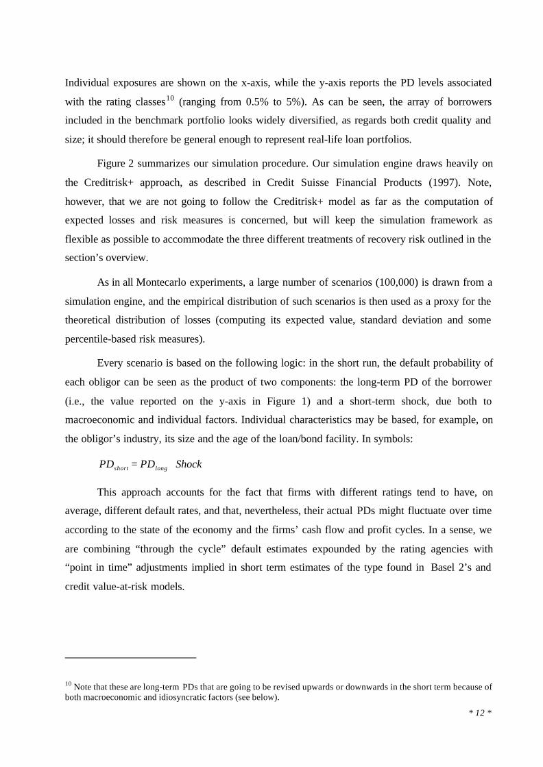
Figure 2 summarizes our simulation procedure. Our simulation engine draws heavily on

the Creditrisk+ approach, as described in Credit Suisse Financial Products (1997). Note,

however, that we are not going to follow the Creditrisk+ model as far as the computation of

expected losses and risk measures is concerned, but will keep the simulation framework as

flexible as possible to accommodate the three different treatments of recovery risk outlined in the

section’s overview.

As in all Montecarlo experiments, a large number of scenarios (100,000) is drawn from a

simulation engine, and the empirical distribution of such scenarios is then used as a proxy for the

theoretical distribution of losses (computing its expected value, standard deviation and some

percentile-based risk measures).

Every scenario is based on the following logic: in the short run, the default probability of

each obligor can be seen as the product of two components: the long-term PD of the borrower

(i.e., the value reported on the y-axis in Figure 1) and a short-term shock, due both to

macroeconomic and individual factors. Individual characteristics may be based, for example, on

the obligor’s industry, its size and the age of the loan/bond facility. In symbols:

ShockPDPD longshort ⋅=

This approach accounts for the fact that firms with different ratings tend to have, on

average, different default rates, and that, nevertheless, their actual PDs might fluctuate over time

according to the state of the economy and the firms’ cash flow and profit cycles. In a sense, we

are combining “through the cycle” default estimates expounded by the rating agencies with

“point in time” adjustments implied in short term estimates of the type found in Basel 2’s and

credit value-at-risk models.

10 Note that these are long-term PDs that are going to be revised upwards or downwards in the short term because ofboth macroeconomic and idiosyncratic factors (see below).

* 13 *

0%

1%

2%

3%

4%

5%

6%

0 5 10 15

EXPOSURE (thousand euros)

PR

OB

AB

ILIT

Y O

F D

EF

AU

LT

Figure 1: PD and exposure of the 250 loans included in the benchmark portfolio

* 14 *

Gamma distributionfor idiosincratic

noise

Gamma distributionfor background factor

)( 2211 xwxw �x2

x1

=x

1.0%2.0%0.5%2.0%1.0%1.0%1.0%2.0%…2.0%0.5%2.0%1.0%

1.3%2.6%0.7%2.6%1.3%1.3%1.3%2.6%…2.6%0.7%2.6%1.3%

$

5. Loop 100,000 times

3. Based on the adjusted PDs, draw the borrowers

defaulting in this scenario

1. Draw a backgroundfactor and some noise from 2

gamma distributions

2. Use macro factor and noise to adjust the 250 long term PDs to their

conditional values

4. Based on recovery ratescompute lossesand file them

Figure 2: the simulation engine used in our experiment

More specifically, the short-term shock can be thought of as the weighted sum of two

random components, both drawn from independent gamma distributions with mean equal to

one11: x1 represents a background factor that is common to all the borrowers in the portfolio (the

risk of an economic downturn affecting all bank customers), while x2 is different for every

obligor, and represents idiosyncratic risk:

2211 xwxwShock +=

Note that, according to this framework, a recession would bring about a very high value

for x1 which, after being combined with the individual components (the x2s), would significantly

increase the short term PDs of most borrowers, bringing them above their average long-term

values. This would make the bank’s portfolio more vulnerable to default risk, since the actual

number of defaults experienced over the following year would be higher. Indeed, if we were

11 In this way, the expected short-term PD will be the long-term value associated with each rating class.

* 15 *

simulating all rating changes, the number of downgrades vs. no change or upgrades would

increase as well. This is related to the “procyclicality” effect that may be an important issue

inherent in any rating-based capital requirement standards.

The weights w1 and w2, through which the macroeconomic and individual shocks are

combined, must be set carefully, since they play an important role in the final results. If too

much emphasis is attributed to systemic risk x1, then the short-term PDs of all borrowers would

mechanically respond to the macroeconomic cycle, and defaults would take place in thick

clusters (increasing the variance of bank losses, i.e., the risk that must be faced by bank

shareholders and regulators). Conversely, if a significant weight is given to the idiosyncratic risk

x2, then the defaults by different borrowers would be entirely uncorrelated and the stream of

bank losses over time could appear quite smooth (since individual risks could be diversified

away).

In order to keep things as simple and transparent as possible, we use a simple fifty-fifty

weighting scheme in our simulation. Note that – although it represents an arbitrary choice - this

is not dramatically different from the 33%-66% scheme underlying the new regulatory

framework proposed by the Basel committee in its January 2001 document 12.

We now return to Figure 2, to see how this logic was implemented in our simulation. For

each scenario:

1. A value for the background factor x1 is drawn from a gamma distribution13; this value,

which is common to all borrowers in the portfolio, is combined with an idiosyncratic

noise term (x2, also taken from a gamma), which is different for every obligor.

2. The combination of x1 and x2 is used to shock the long term values of the obligors’ PDs

in order to obtain the short term probabilities that will be used in the following steps.

Note that when x1 is low, most PDs will be revised downwards (as it happens when a

12 In the January 2001 Basel document, default occurs because of changes in a firm’s asset value; these, in turn,follow a standard normal distribution which combines a macro factor (with a weight of about .45) and anidiosyncratic term (with a weight of .89); hence the 33%-66% proportion quoted in the text. However, as noted bymany observers who discussed the Basel proposals, the idiosyncratic component should probably be given moreimportance for small borrowers, while the systematic component should be more relevant for large firms, the creditquality of which tends to depend more heavily on the overall economic cycle. This remark sounds quite correct, yetusing different weights for each borrower, depending on her size, would have made our simulation longer and lesstransparent. Therefore, we decided to stick to the simplest rule, the “fifty-fifty” weighting.13 We use gamma distributions because they are highly skewed to the right, accounting for the fact that defaultprobabilities tend to stay low most of the time, but can increase dramatically in some (rare) extreme scenarios.

* 16 *

healthy economy makes default risk smaller for most borrowers); on the other hand,

when x1 is high, default probabilities will be adjusted according to a more risky economic

environment (see again Figure 2).

3. Based on the adjusted PDs, the computer draws which borrowers will actually default in

this scenario. A loan with a 10% PD is more likely to default than one with a 2% PD.

However, due to the random error, the latter might go bust while the former survives.

This step of the simulation provides us with a list of defaulted borrowers.

4. For each defaulted loan in the list, the amount of losses is computed. This step can be

performed in three different ways, depending on the assumptions concerning LGD. More

details will be given in the following paragraph.

5. The loss amount generated by this scenario is filed, and a new scenario is started.

2.2. The computation of LGDs

The Montecarlo simulation described above was repeated three times, changing the way in

which LGDs were handled. We tested the three different approaches highlighted at the beginning

of this section:

a) First, LGD is deterministic. In this case we simply multiply the exposure of each

defaulted asset by an “average” loss given default. To keep things simple, we use a 30%

LGD for all borrowers, which is also the mean of the beta distribution utilized in

approach (b).

b) Secondly, LGD is stochastic but uncorrelated with default probabilities. In this case,

LGD is separately drawn for each borrower from a beta distribution limited between 10%

and 50%, with mean 30% and with a variance such that 5/9 of all values are bound

between 20% and 40%.

c) Finally, LGD is stochastic and correlated with default probabilities. In this case, we are

still using the same beta distribution as above, but we impose a perfect rank correlation

between the LGD and the background factor x114. For example, when the background

factor x1 takes a very high value (thereby signalling that the economy is facing a

14 In other words, for every possible value x1* of the background factor x1, such that p(x1<x1*)=P, we choose theLGD as the Pth percentile of its (beta) distribution.

* 17 *

recession), the LGDs increase up to 50%; on the other hand, when the economy

improves, LGDs can become as low as 10%.

2.3 Main Results

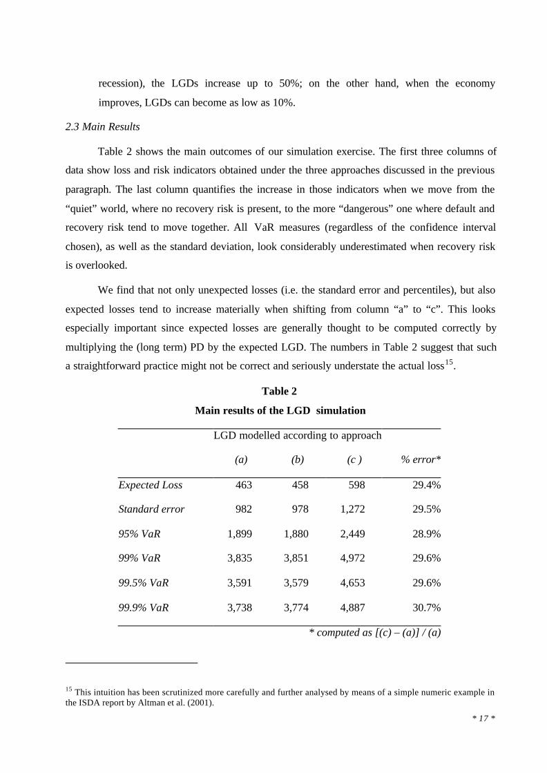
Table 2 shows the main outcomes of our simulation exercise. The first three columns of

data show loss and risk indicators obtained under the three approaches discussed in the previous

paragraph. The last column quantifies the increase in those indicators when we move from the

“quiet” world, where no recovery risk is present, to the more “dangerous” one where default and

recovery risk tend to move together. All VaR measures (regardless of the confidence interval

chosen), as well as the standard deviation, look considerably underestimated when recovery risk

is overlooked.

We find that not only unexpected losses (i.e. the standard error and percentiles), but also

expected losses tend to increase materially when shifting from column “a” to “c”. This looks

especially important since expected losses are generally thought to be computed correctly by

multiplying the (long term) PD by the expected LGD. The numbers in Table 2 suggest that such

a straightforward practice might not be correct and seriously understate the actual loss15.

Table 2

Main results of the LGD simulation

LGD modelled according to approach

(a) (b) (c ) % error*

Expected Loss 463 458 598 29.4%

Standard error 982 978 1,272 29.5%

95% VaR 1,899 1,880 2,449 28.9%

99% VaR 3,835 3,851 4,972 29.6%

99.5% VaR 3,591 3,579 4,653 29.6%

99.9% VaR 3,738 3,774 4,887 30.7%

* computed as [(c) – (a)] / (a)

15 This intuition has been scrutinized more carefully and further analysed by means of a simple numeric example inthe ISDA report by Altman et al. (2001).

* 18 *

Another noteworthy result is that no significant differences arise when we move from

column (a) to (b): in other words, when recovery rates are considered stochastic, but independent

on each other, the law of large numbers ensures that all uncorrelated risks can be effectively

disposed of. A portfolio of 250 loans already looks large enough to exploit this diversification

effect, since its risk measures are not significantly different from the deterministic case. In other

words, it is not uncertainty in recovery rates, but positive correlation, that brings about an

increase in credit risk. Among all possible kinds of correlation, the link between recovery and

default looks to be the most significant and, possibly, dangerous one, since it increases both

unexpected and expected losses. Moreover, the percent error found when moving from (a), or

(b), to (c) is approximately the same (about 30%) for all risk and loss measures (expected and

unexpected losses, percentile-based indices).

Summing up, if PD and LGD were driven by some common causes, then not only the risk

measures based on standard errors and percentiles (i.e., the unexpected losses usually covered

with bank capital), but even the amount of “normal” losses to be expected on a given loan (and

to be shielded through charge-offs and reserves) could be seriously underestimated by most

credit risk models. This reinforces the theoretical relevance of the empirical tests presented in the

following Section.

3. Explaining Aggregate Recovery Rates on Corporate Bond Defaults: Empirical Results

The average loss experience on credit assets is well documented in studies by the various

rating agencies (Moody’s, S&P, and Fitch) as well as by academics16. Recovery rates have been

released for bonds, stratified by seniority, as well as for bank loans. The latter asset class can be

further stratified by capital structure and collateral type. While quite informative, these studies

say nothing about the recovery vs. default correlation. The purpose of this section is to

empirically test this relationship with actual default data from the U.S. corporate bond market

over the last two decades. As Frye (2000a), Altman (2001), Carey and Gordy (2001) and others

point out (see Section 1), there is strong intuition suggesting that default and recovery rates

16 See e.g. Altman and Kishore (1996), Altman and Arman (2002), FITCH (1997, 2001), Moody’s (2000), Standard& Poor’s (2000).

* 19 *

might be correlated. Accordingly, this third Section of our study attempts to explain the link

between the two variables, by specifying rather straightforward statistical models17.

We measure aggregate annual bond recovery rates (henceforth: BRR) by the weighted

average recovery of all corporate bond defaults, primarily in the United States, over the periods

1982-2000 and also for the shorter period, 1987-2000. The weights are based on the market

value of defaulting debt issues of publicly traded corporate bonds18. The logarithm of BRR

(BLRR) is also analysed.

The sample includes annual averages from about 1000 defaulted bonds for which we

were able to get reliable quotes on the price of these securities just after default. We utilize the

database constructed and maintained by the NYU Salomon Center, under the direction of one of

the authors. Our models are both univariate and multivariate, least squares regressions. The

former can explain up to 60% of the variation of average annual recovery rates, while the latter

explain as much as 90%.

The rest of this Section will proceed as follows. We begin our analysis by describing the

independent variables used to explain the annual variation in recovery rates. These include

supply-side aggregate variables that are specific to the market for corporate bonds, as well as

macroeconomic factors (some demand side factors are also discussed). Next, we describe the

results of the univariate analysis. We then describe our multivariate models.

3.1. Explanatory Variables

We proceed by listing several variables we reasoned could be correlated with aggregate

recovery rates. The expected effects of these variables on recovery rates will be indicated by a

+/- sign in parentheses. The exact definitions of the variables we use are:

17 We will concentrate on average annual recovery rates but not on the factors that contribute to understanding andexplaining recovery rates on individual firm and issue defaults. Van de Castle and Keisman (1999) indicate thatfactors like capital structure, as well as collateral and seniority, are important determinants of recovery rates andMadan and Unal (2001) propose a model for estimating risk-neutral expected recovery rate distributions - - notempirically observable rates. The latter can be particularly useful in determining prices on credit derivativeinstruments, such as credit default swaps.18 Prices of defaulted bonds are based on the closing levels on or as close to the default date as possible. Precise-datepricing was only possible in the last ten years, or so, since market maker quotes were not available from the NYUSalomon Center database prior to 1990 and all prior date prices were acquired from secondary sources, primarily theS&P Bond Guides. Those latter prices were based on end-of-month closing bid prices only. We feel that moreexact pricing is a virtue since we are trying to capture supply and demand dynamics which may impact pricesnegatively if some bondholders decide to sell their defaulted securities as fast as possible. In reality, we do notbelieve this is an important factor since many investors will have sold their holdings prior to default or are moredeliberate in their “dumping” of defaulting issues.

* 20 *

BDR (-) The weighted average default rate on bonds in the high yield bond market and its

logarithm (BLDR, -). Weights are based on the face value of all high yield bonds

outstanding each year19.

BDRC (-) One Year Change in BDR.

BOA (-) This is the total amount of high yield bonds outstanding for a particular year (measured

at mid-year in trillions of dollars) and represents the potential supply of defaulted

securities. Since the size of the high yield market has grown in most years over the

sample period, the BOA variable is picking up a time-series trend as well as representing

a potential supply factor.

BDA (-) We also examined the more directly related bond defaulted amount as an alternative for

BOA (also measured in trillions of dollars).

BIR (+) This is the one year return on the Altman-NYU Salomon Center Index of Defaulted

Bonds, a monthly indicator of the market weighted average performance of a sample of

defaulted publicly traded bonds20. This is a measure of the price changes of existing

defaulted issues as well as the “entry value” of new defaults and, as such, is impacted by

supply and demand conditions in this “niche” market.21

GDP (+) The annual GDP growth rate.

GDPC (+) The change in the annual GDP growth rate from the previous year.

GDPI (-) Takes the value of 1 when GDP growth was less than 1.5% and 0 when GDP growth

was greater than 1.5%.

SR (+) The annual return on the S&P 500 stock index.

19 We did not include a variable that measures the distressed, but not defaulted, proportion of the high yield marketsince we do not know of a time series measure that goes back to 1987. We define distressed issues as yielding morethan 1000 basis points over the risk-free 10-year Treasury Bond Rate. We did utilize the average yield spread in themarket and found it was highly correlated (0.67) to the subsequent one year’s default rate and hence did not addvalue (see discussion below). The high yield bond yield spread, however, can be quite helpful in forecasting thefollowing year’s BDR, a critical variable in our model.20 More details can be found in Altman (1991) and Altman and Pompeii (2002). Note that we use two different timeframes in our analyses, 1982-2000 and 1987-2000, because the defaulted bond index return (BIR) has only beencalculated since 1987. We go no earlier than 1982 because there are so few default observations before that year.21 We are aware of the fact that the average recovery rate on newly defaulted bond issues could influence the level ofthe defaulted bond index and vice-versa. The vast majority of issues in the index, however, are usually comprised ofbonds that have defaulted in prior periods. And, as we will see, while this variable is significant on an univariatebasis and does improve the overall explanatory power of the model, it is not an important contributor. We couldonly introduce this variable in the 1987-2000 regression.

* 21 *

SRC (+) The change in the annual return on the S&P 500 stock index from the previous year.

3.2. The Basic Explanatory Variable: Default Rates

It is clear that the supply of defaulted bonds is most vividly depicted by the aggregate

amount of defaults and the rate of default. Since virtually all public defaults most immediately

migrate to default from the non-investment grade or “junk” bond segment of the market, we use

that market as our population base. The default rate is the par value of defaulting bonds divided

by the total amount outstanding, measured at face values. Table 3 shows default rate data from

1978-2001 as well as the weighted average annual recovery rates (our dependent variable) and

the default loss rate (last column). Note that the average annual recovery is 41% and the

weighted average annual loss rate to investors is 3.16%22.

Table 3

22 The loss rate is impacted by the lost coupon at default as well as the more important lost principal.

DEFAULT RATES AND LOSSES (1978 - 2001)

PAR VALUE PAR VALUEOUTSTANDING (a) OF DEFAULT DEFAULT WEIGHTED PRICE WEIGHTED

YEAR ($ MMs) ($ MMs) RATE (%) AFTER DEFAULT COUPON (%)2001 $649,000 $63,609 9.80% $25.5 9.18%2000 $597,200 $30,295 5.07% $26.4 8.54%1999 $567,400 $23,532 4.15% $27.9 10.55%1998 $465,500 $7,464 1.60% $35.9 9.46%1997 $335,400 $4,200 1.25% $54.2 11.87%1996 $271,000 $3,336 1.23% $51.9 8.92%1995 $240,000 $4,551 1.90% $40.6 11.83%1994 $235,000 $3,418 1.45% $39.4 10.25%1993 $206,907 $2,287 1.11% $56.6 12.98%1992 $163,000 $5,545 3.40% $50.1 12.32%1991 $183,600 $18,862 10.27% $36.0 11.59%1990 $181,000 $18,354 10.14% $23.4 12.94%1989 $189,258 $8,110 4.29% $38.3 13.40%1988 $148,187 $3,944 2.66% $43.6 11.91%1987b $129,557 $7,486 5.78% $75.9 12.07%1986 $90,243 $3,156 3.50% $34.5 10.61%1985 $58,088 $992 1.71% $45.9 13.69%1984 $40,939 $344 0.84% $48.6 12.23%1983 $27,492 $301 1.09% $55.7 10.11%1982 $18,109 $577 3.19% $38.6 9.61%1981 $17,115 $27 0.16% $12.0 15.75%1980 $14,935 $224 1.50% $21.1 8.43%1979 $10,356 $20 0.19% $31.0 10.63%1978 $8,946 $119 1.33% $60.0 8.38%

ARITHMETIC AVERAGE 1978-2001: 3.23% $40.54 11.14%WEIGHTED AVERAGE 1978-2001: 4.35%

Notes(a) Excludes defaulted issues.Source: Authors' Compilations and various dealer price quotes.(b) Includes Texaco Inc., which was a unique Chapter 11 bankruptcy, with a face value of over $ 3 billion and an outlierrecovery rate of over 80%. Our models do not include this one firm's influe. Without Texaco the default rate is 1.34%and the recovery rate is 62%.

* 22 *

3.3. The Demand and Supply of Distressed Securities

The principal purchasers of defaulted securities, primarily bonds and bank loans, are

niche investors called distressed asset or alternative investment managers - also called

“vultures.” Prior to 1990, there was little or no analytic interest in these investors, indeed in the

distressed debt market, except for the occasional anecdotal evidence of performance in such

securities. Altman (1991) was the first to attempt an analysis of the size and performance of the

distressed debt market and estimated, based on a fairly inclusive survey, that the amount of funds

under management by these so-called vultures was at least $7.0 billion in 1990 and if you

include those investors who did not respond to the survey and non-dedicated investors, the total

was probably in the $10-12 billion range. Cambridge Associates (2001) estimated that the

amount of distressed assets under management in 1991 was $6.3 billion. Estimates since 1990

indicate that the demand did not rise materially until 2000-2001, when our latest estimate is a

total demand for distressed securities of $40-45 billion as of December 31, 2001 (see Altman and

Pompeii, 2002).

On the supply side, the last decade has seen the amounts of distressed and defaulted

public and private bonds and bank loans grow dramatically in 1990-1991 to as much as $300

billion (face value) and $200 billion (market value), then recede to much lower levels in the

1993-1998 period and grow enormously again in 2000-2001 to the unprecedented levels of $650

billion (face value) and almost $400 billion market value. These estimates are based on

calculations in Altman and Pompeii (2002) from periodic, not continuous, market calculations

and estimates.23

On a relative scale, the ratio of supply to demand of distressed and defaulted securities

was something like ten to one in both 1990-1991 and also in 2000-2001. Dollarwise, of course,

the amount of supply side money dwarfed the demand in both periods. And, as we will show, the

price levels of new defaulting securities was relatively very low in both periods - at the start of

the 1990’s and again at the start of the 2000 decade.

23 Defaulted bonds and bank loans are relatively easy to define and are carefully documented by the rating agenciesand others. Distressed securities are defined here as bonds selling at least 1000 basis points over comparablematurity Treasury Bonds (we use the 10-year T-Bond rate as our benchmark). Privately owned securities, primarilybank loans, are estimated as 1.5-1.8 x the level of publicly owned distressed and defaulted securities based onstudies of a large sample of bankrupt companies (Altman and Pompeii, 2002).

* 23 *

3.4. Univariate Models

We begin the discussion of our results with the univariate relationships between recovery

rates and the explanatory variables described in the previous section. Table 4 displays the results

of the univariate regressions carried out using these variables.

Table 4: Univariate Regressions, 1982-2000

Variables Explaining Annual Recovery Rates on Defaulted Corporate BondsCoefficients and T-Ratios (in parentheses)Regression # (1) (2) (3) (4) (5) (6) (7) (8) (9) (10)R-Squared 0.45 0.49 0.58 0.60 0.51 0.52 0.20 0.23 0.46 0.54Adj. R-Squared 0.42 0.46 0.56 0.58 0.48 0.49 0.15 0.18 0.43 0.51Dependent Variable:BRR X X X X X BLRR X X X X X Explanatory Variables:Constant 0.51 -0.67 0.01 -1.94 0.43 -0.87 0.49 -0.72 0.49 -0.71

(17.40) (-9.55) (0.10) (-9.12) (24.01) (-19.39) (12.83) (-7.70) (19.16) (-12.01)

BDR -2.62 -6.82(-3.73) (-4.04)

BLDR -0.11 -0.28(-4.86) (-5.05)

BDRC -2.99 -7.51(-4.19) (-4.25)

BOA -0.29 -0.76(-2.06) (-2.23)

BDA -8.53 -23.16-3.78 -4.48

GDP

GDPC

GDPI

SR

SRC

Spread

* 24 *

Table 4: Univariate Regressions, 1982-2000 - continued

Variables Explaining Annual Recovery Rates on Defaulted Corporate BondsCoefficients and T-Ratios (in parentheses)Regression # (11) (12) (13) (14) (15) (16) (17) (18) (19) (20) (21) (22)R-Squared 0.03 0.03 0.16 0.14 0.16 0.17 0.02 0.04 0.02 0.05 0.10 0.12Adj. R-Squared -0.02 -0.03 0.11 0.09 0.11 0.12 -0.04 -0.01 -0.04 0.00 0.04 0.06Dependent Variable:BRR X X X X X X BLRR X X X X X X Explanatory Variables:Constant 0.39 -0.96 0.42 -0.89 0.46 -0.80 0.41 -0.95 0.43 -0.89 0.52 -0.63

(7.81) (-7.66) (18.00) (-15.02) (15.48) (-10.96) (10.88) (-10.19) (16.82) (-14.27) (7.12) (-3.52)

BDR

BLDR

BDRC

BOA

BDA

GDP 1.00 2.30(0.77) (0.70)

GDPC 1.76 4.11(1.78) (1.65)

GDPI -0.09 -0.22(-1.78) (-1.84)

SR 0.11 0.43(0.56) (0.88)

SRC 0.08 0.31(0.62) (0.99)

Spread -1.94 -5.27(-1.35) (-1.49)

These univariate regressions, and the multivariate regressions discussed in the following

section, were calculated using both the recovery rate (BRR) and the natural log (BLRR) of the

recovery rate as the dependent variables. Both results are displayed in Table 4, as signified by an

“x” in the corresponding row.

We examine the simple relationship between bond recovery rates and bond default rates

for the period 1982-2000 (there simply are too few default observations in the 1978-1981

period). Table 4 and Figure 3 show several regressions between the two fundamental variables

and we find that one can explain about 45% of the variation in the annual recovery rate with the

level of default rates (this is the linear model, regression 1) and as much as 60%, or more, with

* 25 *

the quadratic and power24 relationships (regressions 3 and 4). Hence, our basic thesis that the rate

of default is a massive indicator of the likely average recovery rate amongst corporate bonds

appears to be substantiated25.

The other univariate results show the correct sign for each coefficient, but not all of the

relationships are significant. BDRC is highly negatively correlated with recovery rates, as

shown by the very significant t-ratios, although the t-ratios and R-squared values are not as

significant as those for BLDR. BOA and BDA are, as expected, both negatively correlated with

recovery rates with BDA being more highly negatively correlated than BOA on a univariate

basis. Macroeconomic variables did not explain as much of the variation in recovery rates as the

corporate bond market variables explained; we will come back to these relationships in the next

paragraphs.

24 The power relationship (BRR = exp[b0]×BDRb1) can be estimated using the following equivalent equation: BLRR= b0 + b1×BLDR (“power model”).25 Such an impression is strongly supported by a -80% rank correlation coefficient between BDR and BRR(computed over the 1982-2001 period; however, the same value holds for the reduced 1987-2000 window used inthe following paragraphs). Note that rank correlations represent quite a robust indicator, since they do not dependupon any specific functional form (e.g., log, quadratic, power, etc.).

Figure 3

Recovery Rate/Default Rate AssociationAltman Defaulted Bonds Data Set (1982-2000)

Dollar Weighted Average Recovery Rates to Dollar Weighted Average Default Rates

1997

1984

1996

19931983

1987

1994

1998

1985

1995

1988

1982

1992

1986

1989

19992000

1990

1991

y = -2.617x + 50.9R2 = 0.4498

y = -11.181Ln(x) + 52.332R2 = 0.5815

y = 0.5609x2 - 8.7564x + 60.61R2 = 0.6091

y = 52.739x-0.2834

R2 = 0.6004

20

25

30

35

40

45

50

55

60

65

0 2 4 6 8 10 12

Default Rate (%)

Rec

over

y R

ate

(%)

* 29 *

3.5. Multivariate Models

We now specify models to explain recovery rates that are somewhat more complex by

including several additional variables to the important default rate measure. The basic structure

of our most successful models is:

BRR = f(BDR, BDRC, BOA or BDA, BIR)

Some macroeconomic variables will be added to this basic structure, to test their effect on

recovery rates.

We have constructed two simple regression structures in order to explain recovery rate

results and to predict 2001 rates. One set is for the longer 1982-2000 period and the other is for

the 1987-2000 period26. Both sets involve linear and log-linear structures for the two key

variables – recovery rates (dependent) and default rates (explanatory) with the log-linear

relationships somewhat more significant. These results appear in Table 5 and 6; regressions 1

through 4 build the “basic models”, while macro variables are added in the following rows.

3.6. The Results for 1987-2000

Table 5 regressions 1-4 present our results for the “basic” models. Note that most, but

not all, of the variables are quite significant based on their t-ratios. The overall accuracy of the fit

goes from 84% (76% adjusted R-square) for the strictly absolute value of all variables

(regression 1) to 88% (83% adjusted) when the dependent variable (regression 2) is specified in

natural logs, to the same 88% (regression 3) when only the primary independent variable (default

rates – BLDR) is specified in natural logs to as much as 91% (unadjusted) and 87% (adjusted) R-

squares where both the primary dependent (BLRR) and explanatory variable (BLDR) are

expressed in natural logs (regression 4).

26 As concerns the BIR variable, univariate regressions were carried out over the 1987-2000 period, as this index isnot available in previous years: we found positive coefficients both for BRR and its log, with t-test values of about2.3.

* 30 *

Table 5: Multivariate Regressions 1987 –2000

Variables Explaining Annual Recovery Rates on Defaulted Corporate BondsCoefficients and T-Ratios (in parentheses)Regression # (1) (2) (3) (4) (5) (6) (7) (8) (9) (10)R-Squared 0.84 0.88 0.88 0.91 0.81 0.89 0.84 0.91 0.76 0.78Adj. R-Squared 0.76 0.83 0.83 0.87 0.73 0.84 0.74 0.86 0.65 0.68Dependent Variable:BRR X X X X X BLRR X X X X X Explanatory Variables:Constant 0.56 -0.55 0.16 -1.55 0.49 -1.29 0.58 -1.54 0.37 -1.02

(11.65) (-5.33) (2.12) (-9.27) (16.43) (-4.51) (4.89) (-8.41) (5.52) (-6.36)

BDR -2.02 -5.28 -1.04 -2.20(-3.40) (-4.15) (-1.29) (-2.01)

BLDR -0.09 -0.22 -0.13 -0.21(-4.41) (-5.18) (-1.96) (-3.51)

BDRC -1.17 -3.06 -1.31 -3.51 -1.26 -3.45 -1.13 -3.51 -1.82 -4.85(-1.64) (-2.01) (-2.26) (-2.82) (-1.65) (-2.45) (-1.48) (-2.66) (-2.29) (-2.55)

BOA -0.26 -0.67 -0.23 -0.59 -0.25 -0.60 -0.33 -0.85(-2.08) (-2.52) (-2.16) (-2.60) (-1.66) (-2.23) (-2.04) (-2.18)

BDA -4.37 -10.60-1.56 -1.84

BIR 0.11 0.26 0.08 0.20 0.15 0.33 0.10 0.21 0.18 0.43(1.29) (1.44) (1.18) (1.28) (1.81) (2.14) (0.94) (1.10) (1.61) (1.63)

GDP -0.56 0.41 3.95 9.81(-0.20) (0.11) (2.17) (2.26)

GDPC

GDPI

SR

SRC

Spread

* 31 *

Table 5: Multivariate Regressions 1987 –2000 – ContinuedFigure 7 – Multivariate Regressions 1987-2000 (Continued)Variables Explaining Annual Recovery Rates on Defaulted Corporate BondsCoefficients and T-Ratios (in parentheses)Regression # (11) (12) (13) (14) (15) (16) (17) (18) (19) (20)R-Squared 0.85 0.92 0.84 0.91 0.84 0.93 0.84 0.92 0.85 0.92Adj. R-Squared 0.75 0.86 0.74 0.86 0.74 0.88 0.74 0.87 0.75 0.87Dependent Variable:BRR X X X X X BLRR X X X X X Explanatory Variables:Constant 0.56 -1.56 0.56 -1.56 0.55 -1.54 0.56 -1.53 0.49 -2.15

(11.29) (-8.91) (10.60) (-7.17) (10.23) (-9.54) (11.03) (-8.93) (4.50) (-3.28)

BDR -2.16 -2.06 -1.98 -2.05 -3.71(-3.39) (-2.88) (-3.07) (-3.22) (-1.39)

BLDR -0.22 -0.22 -0.21 -0.21 -0.32(-5.00) (-4.44) (-4.98) (-4.95) (-2.73)

BDRC -1.64 -4.23 -1.17 -3.52 -1.20 -3.73 -1.12 -3.74 -0.79 -3.27(-1.70) (-2.36) (-1.55) (-2.65) (-1.58) (-3.08) (-1.44) (-2.87) (-0.85) (-2.56)

BOA -0.25 -0.58 -0.26 -0.58 -0.26 -0.61 -0.26 -0.58 -0.29 -0.58(-1.98) (-2.44) (-1.90) (-2.37) (-1.98) (-2.78) (-1.98) (-2.48) (-2.11) (-2.57)

BDA

BIR 0.08 0.16 0.11 0.20 0.10 0.17 0.12 0.15 0.02 0.02(0.87) (0.91) (1.21) (1.20) (1.16) (1.14) (1.23) (0.89) (0.16) (0.10)

GDP

GDPC -1.33 -1.87(-0.75) (-0.58)

GDPI 0.01 0.01(0.13) (0.09)

SR 0.03 0.26(0.29) (1.31)

SRC -0.02 0.13(-0.27) (0.80)

Spread 2.70 4.55(0.65) (0.95)

* 32 *

Table 6: Multivariate Regressions 1982 -2000

Variables Explaining Annual Recovery Rates on Defaulted Corporate BondsCoefficients and T-Ratios (in parentheses)Regression # (1) (2) (3) (4) (5) (6) (7) (8) (9) (10)R-Squared 0.77 0.82 0.83 0.87 0.74 0.84 0.78 0.88 0.66 0.68Adj. R-Squared 0.73 0.79 0.80 0.84 0.69 0.81 0.71 0.85 0.59 0.62Dependent Variable:BRR X X X X X BLRR X X X X X Explanatory Variables:Constant 0.53 -0.61 0.20 -1.46 0.49 -1.20 0.54 -1.55 0.46 -0.79

(20.03) (-10.46) (2.75) (-9.17) (21.99) (-5.01) (12.89) (-9.45) (13.06) (-9.29)

BDR -1.62 -4.36 -0.69 -1.75(-3.02) (-3.69) (-0.94) (-2.71)

BLDR -0.07 -0.19 -0.11 -0.23(-4.16) (-4.74) (-1.96) (-4.92)

BDRC -2.02 -4.92 -1.88 -4.67 -2.12 -4.81 -2.03 -4.64 -2.63 -6.60(-3.49) (-3.87) (-3.75) (-4.20) (-3.46) (-3.96) (-3.40) (-4.34) (-3.98) (-4.17)

BOA -0.22 -0.58 -0.19 -0.51 -0.20 -0.40 -0.26 -0.69(-2.72) (-3.33) (-2.67) (-3.27) (-2.31) (-2.42) (-2.56) (-2.83)

BDA -4.94 -11.73(-2.20) (-2.55)

GDP -0.32 -2.42 0.87 2.06(-0.37) (-1.50) (0.98) (0.97)

GDPC

GDPI

SR

SRC

Spread

* 33 *

Table 6: Multivariate Regressions 1982 –2000 - continuedFigure 8 – Multivariate Regressions 1982-2000 (Continued)Variables Explaining Annual Recovery Rates on Defaulted Corporate BondsCoefficients and T-Ratios (in parentheses)Regression # (11) (12) (13) (14) (15) (16) (17) (18) (19) (20)R-Squared 0.78 0.88 0.77 0.87 0.78 0.89 0.78 0.89 0.71 0.79Adj. R-Squared 0.71 0.85 0.71 0.83 0.72 0.86 0.71 0.86 0.66 0.75Dependent Variable:BRR X X X X X BLRR X X X X X Explanatory Variables:Constant 0.53 -1.51 0.53 -1.51 0.52 -1.47 0.53 -1.47 0.39 -2.11

(19.38) (-9.54) (19.25) (-7.79) (15.95) (-9.88) (18.81) (-9.93) (6.29) (-5.32)

BDR -1.66 -1.68 -0.20 -1.56 -1.60 -3.80(-2.95) (-2.66) (-4.30) (-2.79) (-2.88) (-2.69)

BLDR -0.20 -0.18 -0.18 -0.28(-5.10) (-4.76) (-5.03) (-3.78)

BDRC -2.15 -5.53 -2.04 -4.74 -2.06 -4.83 -2.07 -4.89 -1.32 -4.03(-3.10) (-4.48) (-3.38) (-4.11) (-3.47) (-4.63) (-3.44) (-4.70) (-1.60) (-2.69)

BOA -0.21 -0.48 -0.22 -0.50 -0.22 -0.51 -0.20 -0.43(-2.58) (-3.14) (-2.63) (-3.15) (-2.66) (-3.52) (-2.39) (-2.85)

BDA

GDP

GDPC -0.24 -1.84(-0.35) (-1.43)

GDPI 0.01 0.03(0.19) (0.46)

SR 0.06 0.33(0.61) (1.79)

SRC 0.04 0.23(0.50) (1.85)

Spread 3.30 3.77(1.63) (1.33)

* 34 *

Figure 4 - Actual vs. Estimated Recovery Rates on Defaulted Corporate Bonds

1987

1988

1989

1990

1991

1992

1993

19941995

19961997

1998

19992000

1987

1988

1989

1990

1991

1992

1993

1994

1995

1996

1997

1998

1999

2000

2001 (22%)2001 (23%)

20%

25%

30%

35%

40%

45%

50%

55%

60%

65%

0% 2% 4% 6% 8% 10% 12%

Default Rate

Rec

ove

ry R

ate

Observed Estimated

* 35 *

The actual model with the highest explanatory power and lowest “error” rates is the

power model27 in regression 4 of Table 5. We see that all of the four explanatory variables have

the expected sign (negative for BLDR, BDRC, and BOA and positive for BIR) and are

significant at the 5% or 1% level, except for the Defaulted Bond Index (BIR) which has the

appropriate sign (+) but a less meaningful t-ratio28. BLDR and BDRC are extremely significant,

showing that the level and change in the default rate are highly important explanatory variables

for recovery rates. Indeed the variables BDR (and BLDR) explain up to 57% (unadjusted) and

53% (adjusted) of the variation in BRR simply based on a linear or log-linear association. The

size of the high yield market also performs very well and adds about 8% to the explanatory

power of the model. When we substitute BDA for BOA, the explanatory power of multivariate

model drops somewhat to 0.89 (unadjusted) and 0.84 (adjusted) R-squared. Still, the sign of

BDA is correct (+) and the t-ratio is quite high (1.84 – see regression 6 of Table 5). Indeed, on a

univariate basis, BDA is actually far more significant than BOA (see Table 4).

Figure 4 shows, graphically, the results for the Table 5 regression 4 structure, by

comparing the actual Recovery Rate vs. the estimated rates (designated by a “+” sign) for 1987-

2000. Note the extremely close accuracy in almost every year between the actual and estimated

rates. Figure 4 also shows how our multivariate regressions can be used to estimate the 2001

expected recovery rate, given certain assumptions about the independent variables and the time

frame for the regressions. Specifically, assuming default rates for 2001 of 8.5% (or 10%)29, a

change in default rates compared to 2000’s 5.1% of 3.44% (or 4.94%), a BIR of 18.0% (the rate

of return as of August, 2001), a BOA of $630 billion (midyear 2001) or a BDA of 8.5%-10% of

the high yield bond market, this results in an estimated recovery rate of 22-23% When we

substitute BDA for BOA, the estimates for 2001 recovery rates are 20% assuming an 8.5%

default rate and 18% assuming a 10% default rate. The actual recovery rate in 2001 was 25%

(including one large unique bankruptcy – FINOVA – or 21% - without FINOVA – see Altman

and Arman, 2002); so our estimates were very close to the actual.

27 Like its univariate cousin, the multivariate power model can be written using logs. E.g., BLRR = b0 + b1×BLDR +b2×BDRC + b3×BIR + b4×BOA becomes BRR = exp[b0] × BDRb1 × exp[b2×BDRC + b3×BIR + b4×BOA]and takes its name from BDR being raised to the power of its coefficient.28 BIRs t-ratio is only significant at the 0.25 level. Without the BIR variable, the R-squared measures are slightlylower at 90% (unadjusted ) and 87% (adjusted). On a univariate basis, the BIR is significant with a t-ratio of 2.34and explains 25% of the variation in BRR.29 These were Altman’s (8.5%) and Moody’s (10.0%) default rates estimates for 2001 made at the beginning of theyear. More recent estimates are higher given the impact from the September 11, 2001 tragedy, and the final defaultrate in 2001 was 9.8%.

* 36 *

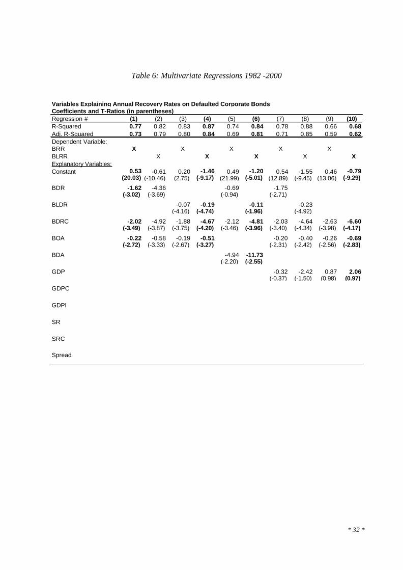
3.7. The Results for 1982-2000 and Autocorrelation Tests

Table 6 regressions 1-4 show the same regression structures as Table 5 regressions 1-4,

only the sample period is for 1982-2000 and the models do not include the BIR variable.

Regression 1 of Table 6 shows that all three explanatory variables are significant at the 1% or

5% level with high t-ratios. All have the correct sign, indicating that recovery rates are

negatively correlated with default rates, the change in default rates and the size of the high yield

bond market. The R-squared of this straightforward, linear regression is 0.77 (0.73 adjusted).

Finally, as with the shorter time period, the highest R-squared explanatory model for the longer

time period uses the log specification for both BLRR and BLDR, which raises the unadjusted R-

squared to 0.87 (Table 6, regression 4). These results are slightly lower than for the longer time

frame (1982-2000), but still very meaningful. Hence, we are quite optimistic that the variable

set, while probably not optimal, can be used to explain and predict recovery rates in the

corporate defaulted bond market.

We do observe a few clusters of recovery rates in such years as 1994-1995,1996-1997

and 1999-2000 (see Figures 3 and 4) so we test for autocorrelation of the residuals. The resulting

Durbin-Watson statistics did not show any autocorrelation problems and either reject the

assumption or find the tests inconclusive.

3.8. Macroeconomic Variables

While we are pleased with the accuracy and explanatory power of the regressions

described above, we were not very successful in our attempts to include several fundamental

macroeconomic factors. We assessed these factors both on a univariate as well as a value-added

basis for our multivariate structures. We are somewhat surprised by the low contributions of

these variables since there are several models that have been constructed that utilize macro-

variables, apparently significantly, in explaining annual default rates30.

Despite the fact that the growth rate in annual GDP is significantly negatively correlated

with the bond default rate, i.e., -0.67 for the period 1987-2000 and -0.50 for 1982-2000, the

univariate correlation between recovery rates (BRR) and GDP growth is relatively low (see

Table 4); the sign (+) is appropriate, however. Note that the GDP growth variable has a -0.02

30 See e.g. Fons (1991), Jonsson and Fridson (1996), Moody’s (1999), Fridson, Garman, and Wu (1997), Helwegeand Kleiman (1997).

* 37 *

and -0.03 adjusted R-squared with BRR and BLRR (regressions 11 and 12), and a positive but

not very significant relationship with recovery rates (R-squared 0.14 - 0.16 unadjusted) when we

utilize the change in GDP growth (GDPC, regressions 13 and 14).

Furthermore, when we introduce GDP and GDPC to our existing multivariate structures

(Tables 5 and 6), not only are they not significant, but they have a counterintuitive sign

(negative). The news is not all bad with respect to the multivariate contribution of the GDP

variable. When we substitute GDP for BDR in our most successful regressions (see Tables 5

and 6, regressions 9 and 10), we do observe that GDP is significant at .05 level and the sign (+)

is correct.

BRR = f (GDP, BDRC, BIR, BOA)

explains 0.76 of BRR and 0.78 of BLRR. This compares to 0.84 and 0.88 when we use BDR

instead of GDP. No doubt, the high negative correlation (-0.67) between GDP and BDR

eliminates the possibility of using both in the same multivariate structure.

To try and circumvent this problem, we used a technique similar to Helwege and Kleiman

(1997): they postulate that, while a change in GDP of say 1% or 2% was not very meaningful in

explaining default rates when the base year was in a strong economic growth period, the same

change was meaningful when the new level was in a weak economy. Following their approach,

we built a dummy variable (GDPI) which takes the value of 1 when GDP grows at less than

1.5% and 0 otherwise.

Table 4 shows the univariate GDPI results, while Table 5 and Table 6 (regression 14) add

the “dummy” variable GDPI to the “power” models discussed earlier. Note that the univariate

results show a somewhat significant relationship with the appropriate sign (negative). When the

economy grows less than 1.5%, we find that this macroeconomic indicator explains about 0.16 to

0.17 (unadjusted) and 0.11 and 0.12 (adjusted) of the change in recovery rates. The multivariate

model with GDPI, however, does not add any value to our already very high explanatory power

and the sign (+) now is not appropriate. No doubt, the fact that GDP growth is highly correlated

with default rates, our primary explanatory variable, impacts the significance and sign of the

GDP indicator (GDPI) in our multivariate model.

We also postulated that the return of the stock market could impact prices of defaulting

bonds in that the stock market represented investor expectations about the future. Table 5 and 6

regressions 15-18 show the association between the annual S&P 500 Index stock return (SR)

* 38 *

(and its change, SRC) and recovery rates. Note the extremely low univariate R-squared

measures and the insignificant t-ratios in the multivariate model, despite the appropriate signs.

4. The LGD/PD link and the procyclicality effects

Our findings also have implications for the issue of procyclicality. Procyclicality involves

the regulatory capital impact for expected and unexpected losses based on the rating distribution

of bank portfolios. Since average ratings and default rates are sensitive to business cycle effects,

this makes the new internal ratings-based approach to regulatory capital more dependent on the

cycle, increasing capital charges, and limiting credit supply, right when the economy is slowing.

Since we found a significant correlation between macroeconomic measures and bond

rates/defaults, we might expect that low recovery rates when defaults are high would exacerbate

bank loan losses (LGD) in those periods31.

When banks adopting the so-called “advanced” IRB approach are free to estimate their

own severity rates, with some constraints, they might tend to adjust these estimates according to

the economic cycle. As default rates increase, and ratings worsen, LGDs would be revised

upwards, making Basel capital even more procyclical than expected.

To assess the impact of such a mechanism, we carry out a simulation based on the

evolution over a 20-year period of a standard portfolio of bank loans 32. The initial composition

was chosen arbitrarily, based upon some estimates carried out by the Bank of Italy on a sample

of Italian banks33 (Marullo-Reedtz, 2000). All loans are assumed to have a 3-year maturity.

From 1981 until 2000, the bank’s portfolio mix changes accordingly to S&P transition

matrices34 (based on static pools); rates on new loans are revised to compensate for their changes

in riskiness, yet margins earned on “old loans” remain unchanged (since the loans have a three-

year maturity, this means that only 1/3 of the loans can be re-priced). Losses emerge according

31 Note that we do not find much of a relationship between GDP growth and recovery rates. However, when wesubstitute GDP growth for our primary bond default rate variable, the multivariate results are quite meaningful,albeit with a lower explanatory power than the one obtained with the BDR variable.32 These results are based upon the simulation engine presented in detail in Resti (2002).33 Based on Standard & Poor’s rating classes, the composition can be summarized as follows: AAA: 8.0%; AA:8.0%; A: 9.0% ; BBB: 23.0% , BB: 40.0%; B 9.0%; CCC 3.0% . The use of data on rated bonds would probablyhave introduced a severe bias, as the average credit quality of bonds, in the aggregate, tends to be better than that ofbank loans.34 Standard & Poor’s (2001). We are aware that bond data and through-the-cycle ratings are not fully apt to representthe behaviour of bank loans; yet, we believe that such limitations are outweighed by the benefits of using public,certified, long-term data as those supplied by S&P.

* 39 *

to the empirical default rates recorded by S&P and the loans’ LGD (given a 50% LGD, a 100€

default means a 50€ loss).

Capital requirements are measured according to the “corporate exposures” curve

presented in Basel Committee on Bank Supervision (2001a, the so-called “consultative package

two”); the new curve for corporate exposures, circulated in November 2001 (Basel Committee

on Bank Supervision, 2001b), is used as well.

Figure 5: a simulation exercise on the pro-cyclical effects of the PD/LGD correlation

Our simulation contrasts two different scenarios. In the former, a standard 50% LGD is

used for all loans (as in the “foundation” approach, where severities on unsecured, senior loans

are fixed by regulators). In the latter, LGDs fluctuate between 60% (in high default years) and

(b) Simulation results for corporate loans: change in portfolio size

-30%

-20%

-10%

0%

10%

20%

30%

40%

1981 1984 1987 1990 1993 1996 1999

CP2, fixed LGD

CP2, 40-60% LGD

Nov01, fixed LGD

Nov01, 40-60% LGD

(a) Background: indicators of the credit quality cycle

0.0%

2.0%

4.0%

1981 1984 1987 1990 1993 1996 1999

-2%

0%

2%4%

6%

8%

Default rate(%) on S&Pdata (lhs)

default rateon portfolio(rhs)

S&P: down-minus up-grades (rhs)

* 40 *

40% (in low default years)35. Note that, as mentioned above, a similar setting may become

realistic when banks move to the advanced IRB approach and start using their own LGD

estimates.

We now turn to Figure 5, where simulation results are summarized:

1. The first panel (a) reports three indicators of the credit quality cycle: the default rate

measured by Standard and Poor’s on US bonds, the default rate experienced by the bank

(given its portfolio mix) and the “net downgrade rate” (downgrades minus upgrades, over

total outstanding issues). Note that scales are inverted, since an increase in these variables

means that the cycle is getting worse. As can be seen, default and downgrade risks fluctuate

up and down in the Eighties, hit a low in the early Nineties, then keep improving in the

following years, although they worsen again towards the end of the decade.

2. The second panel (b) reports a measure of credit availability: the percent change in the loan

portfolio made possible (or necessary) by the evolution of the capital ratios. When the margin

income exceeds credit losses, and/or capital requirements decrease because of a favourable

evolution in the quality mix of the loans, the bank’s capital grows beyond the minimum

requirements: we then compute by how much the loan portfolio could be enlarged; similarly,

when capital charges increase more than net profits would allow, we estimate the reduction

in loans needed to comply with Basel ratios.

Two results are worth mentioning. First, the procyclicality effect is driven more by up-

and downgrades, rather than by default rates; in other words, adjustments in credit supply needed

to comply with capital requirements seem to respond mainly to changes in the structure of

weighted assets, and only to a minor extent to actual credit losses. However this is not true in

1991 when the default rate is exceptionally high. Second, when we let LGDs free to fluctuate

with default rates, the procyclicality effect increases significantly, both for the CP2 curve and

November 2001 curve 36. Moreover, one could also show that bank spreads, too, would become

more volatile (since revisions in short-term LGD estimates would be factored into loan prices)37.

35 We used a second-degree polynomial to model the link between LGDs and empirical default rates, so that LGD is50% when default rates are at their 20-year average (2%), LGD is 60% when default rates hit their 20-yearmaximum (5%) and LGD is 40% when default rates hit their 20-year low (0%).36 Surprisingly enough, the new weight curve for corporate loans proposed in Basel Committee on BankingSupervision (2001b), although it considerably reduces capital requirements in a static sense, would not ease theprocyclicality effect, at least for loan portfolios like our simulated one. The reason for this rather counter-intuitivebehaviour is that under the November 2001 curve, although the increase in weights when moving to an AAA to a

* 41 *

Thus, if a positive correlation between default and recovery risk (like that in Section 3 for

US bonds), were to be confirmed by bank data, the procyclicality effects might be even more

severe than expected. Of course, one might object that the bank in our simulation behaves in a

somewhat myopic way, and that regulation should encourage “advanced” IRB systems to use

long-term average recovery rates (instead of revising them yearly, according to short-term

signals like the current default rate). However, while the use of long-term LGDs would make

procyclicality effects less marked, it would also force banks to maintain a less updated picture of

their risks, thereby trading stability for precision.

5. Concluding remarks

This paper analyzed the link between aggregate default probabilities and the loss given

default on bank loans and corporate bonds, both from a theoretical and an empirical standpoint,

and tried to spot its implications for various credit VaR models as well as for bank regulation and

procyclicality effects. As far as the theoretical aspects are concerned, most of the literature on

credit risk management models and tools treats the recovery rate variable as a function of historic

average default recovery rates (conditioned perhaps on seniority and collateral factors), but in

almost all cases as independent of expected or actual default rates. To us, this appears to be a

rather simplistic and perhaps unrealistic approach: empirical evidence as well as simulations

results suggest more care in dealing with this fundamental aspect of credit risk modeling.

We saw in Section II how simulation results for expected and unexpected losses may

change under three different recovery rate scenarios. We first assumed that recovery is

deterministic (fixed), then that recovery rates are stochastic yet uncorrelated with the probability

of default, and finally that they are stochastic and negatively correlated with default probabilities.

Introducing this third hypothesis prompts a significant increase (30%) both in risk measures

(unexpected losses) and in the expected cost of defaults. The assessment and measurement of

the PD/LGD correlation (if any) therefore turns out to be a pivotal empirical issue.

To this aim, in Section III we examined the recovery rates on corporate bond defaults,

over the period 1982-2000, by means of rather straightforward statistical models. These models

CCC rated loan is lower, smaller quality changes can bring about a sharper rise in capital requirements than theydid under the CP2 function. This would slightly enhance procyclicality in “normal times” (when most ratingchanges affect the middle part of the rating scale); however, the new curve would probably smooth cyclical effectsunder extreme scenarios, when a large part of bank borrowers moves to the bottom grades of the rating scale.37 See Resti (2002) for details.

* 42 *

assign a key role to the supply of defaulted paper (default rates) and explain a substantial

proportion of the variance in bond recovery rates aggregated across all seniority and collateral

levels.

Our results have important implications for just about all portfolio credit risk models, for

markets which depend on recovery rates as a key variable (e.g., securitizations, credit

derivatives, etc.), and for the current debate on the revised BIS guidelines for capital

requirements on bank credit assets. Namely, in Section IV, we have shown that the link between

LGD and PD will possibly bring about a sharp increase in the “procyclicality” effects of the new

Basel Accord, when individual banks are free to use their own severity estimates; actually, if

banks tend to revise such estimates upwards in “bad” times, bank capital and credit supply might

behave even more pro-cyclically than expected.

* 43 *

References

Altman, Edward I., 1989, “Measuring Corporate Bond Mortality and Performance”, Journal ofFinance 44, 909-922.

Altman, Edward I., 2001, “Altman High Yield Bond and Default Study”, Salomon SmithBarney, U.S. Fixed Income High Yield Report, July.

Altman, Edward I., 1991, Distressed Securities, Irwin Publishing (reprinted by Beard Books,1999).

Altman Edward I., and P. Arman, 2002, “Defaults and Returns in the High Yield Bond Market:Analysis Through 2001,” NYU Salomon Center Working Paper, January.

Altman, Edward I. and Brooks Brady, 2002, “Explaining Aggregate Recovery Rates onCorporate Bond Defaults”, NYU Salomon Center, Working Paper Series, January.

Altman, Edward I. and Jason Pompeii, 2002, “The Performance of Defaulted Bonds and BankLoans: 1987-2001”, NYU Salomon Center Working Paper Series, January.

Altman, Edward I. and Vellore M. Kishore, 1996, “Almost Everything You Wanted to KnowAbout Recoveries on Defaulted Bonds”, Financial Analysts Journal,November/December.

Altman, Edward I., Andrea Resti, and Andrea Sironi, 2001, Analyzing and Explaining DefaultRecovery Rates, a Report submitted to ISDA, London, January.

Basel Committee on Banking Supervision, 1999, Credit Risk Modeling: Current Practices andApplications,. Bank for International Settlements, June.

Basel Committee on Banking Supervision, 2001a, “The Basel Capital Accord”, ConsultativePaper, Bank for International Settlements, January.

Basel Committee on Banking Supervision, 2001b, “Potential Modifications to the Committee’sProposals”, Bank for International Settlements, Basel, November.

Black, Fischer and John C. Cox, 1976, “Valuing Corporate Securities: Some Effects of BondIndenture Provisions”, Journal of Finance, 31, 351-367.

Cambridge Associates, LLC, 2001, U.S. Distressed Company Investing, Cambridge, MA.

Carey, Mark and Michael Gordy, 2001, “Systematic Risk in Recoveries on Defaulted Debt,”Unpublished Working Paper presented at the 2001, Financial Management AssociationMeetings, Toronto, October 20.

Credit Suisse Financial Products, 1997, CreditRisk+. A Credit Risk Management Framework ,Technical Document.

Crouhy, Michel, Dan Galai and Robert Mark, 2000, “A Comparative Analysis of Current CreditRisk Models”, Journal of Banking & Finance, 24, 59-117.

Duffie, Darrell and Kenneth J. Singleton, 1999, “Modeling the Term Structures of DefaultableBonds”, Review of Financial Studies, 12, 687-720.

Duffie, Darrell, 1998, “Defaultable Term Structure Models with Fractional Recovery of Par”,Graduate School of Business, Stanford University.

Duffee, Gregory R., 1999, "Estimating the Price of Default Risk", Review of Financial Studies,Spring, 12(1), 197-225.

* 44 *

Eom, Young Ho, Jean Helwege and Jing-zhi Huang, 2001, “Structural Models of CorporateBond Pricing: An Empirical Analysis”, mimeo.

Finger, Chris, 1999, “Conditional Approaches for CreditMetrics Portfolio Distributions”,CreditMetrics Monitor, April.

FITCH, 1997, “Syndicated Bank Loan Recovery Study,” R. Grossman, M. Brennan and Vento,October 22.

FITCH, 2001, “Bank Loan and Bond Recovery Study: 1997-2001,” S. O’Shea, S. Bonelli and R.Grossman, March 19.

Fons, Jerome, 1987, “The Default Premium and Corporate Bond Experience,” Journal ofFinance, vol. 42, No. 1.

Fridson, Martin, Christopher Garman and Chen Wu, “Real Interest Rates and Default Rates onHigh Yield Bonds,” Journal of Fixed Income, September 1977.

Frye, John, 2000a, “Collateral Damage”, Risk, April, 91-94.

Frye, John, 2000b, “Collateral Damage Detected”, Federal Reserve Bank of Chicago, WorkingPaper, Emerging Issues Series, October, 1-14.

Frye, John, 2000c, “Depressing Recoveries”, Risk, November.

Geske, Robert, 1977, “The Valuation of Corporate Liabilities as Compound Options”, Journal ofFinancial and Quantitative Analysis, 12, 541-552.

Gordy, Michael, 2000a, “A Comparative Anatomy of Credit Risk Models”, Journal of Bankingand Finance, January, 119-149.

Gordy, Michael B., 2000b, “Credit VaR Models and Risk-Bucket Capital Rules: AReconciliation,” Working Paper, Federal Reserve Board, March.

Gupton, Greg M., Christopher C. Finger and Mickey Bhatia, 1997, “CreditMetrics - TechnicalDocument”, (New York, J.P.Morgan).

Gupton, Greg M., Daniel Gates and Lea V. Carty, 2000, “Bank Loan Loss Given Default”,Moody’s Investors Service, Global Credit Research, November.

Hamilton, David T., Greg M. Gupton and Alexandra Berthault, 2001, “Default and RecoveryRates of Corporate Bond Issuers: 2000”, Moody’s Investors Service, February.

Hu, Yen-Ting, and William Perraudin, 2002, “The Dependence of Recovery Rates andDefaults”, BirkBeck College, mimeo, February.

Hull, John and Alan White, 1995, “The Impact of Default Risk on the Prices of Options andOther Derivative Securities”, Journal of Banking and Finance, 19, 299-322.

Jarrow, Robert A. and Stuart M. Turnbull, 1995, “Pricing Derivatives on Financial SecuritiesSubject to Credit Risk”, Journal of Finance 50, 53-86.

Jarrow, Robert A., 2001, “Default Parameter Estimation Using Market Prices”, FinancialAnalysts Journal, Vol. 57, No. 5, pp. 75-92.

Jarrow, Robert A., David Lando, and Stuart M. Turnbull, 1997, “A Markov Model for the TermStructure of Credit Risk Spreads”, Review of Financial Studies, 10, 481-523.

Jarrow, Robert, 2000, “Estimating Recovery Rates and (Pseudo) Default Probabilities Implicit inDebt and Equity Prices,” Working Paper , Cornell.

* 45 *

Jokivuolle, Esa and Samu Peura, 2000, “A Model for Estimating Recovery Rates and CollateralHaircuts for Bank Loans”, Bank of Finland Discussion Papers February.

Jones, E., S. Mason and E. Rosenfeld, 1984, “Contingent Claims Analysis of Corporate CapitalStructures: An Empirical Investigation”, Journal of Finance, 39, 611-627.

Kim I.J., K. Ramaswamy, S. Sundaresan, 1993, “Does Default Risk in Coupons Affect theValuation of Corporate Bonds? A Contingent Claims Model”, Financial Management,22, No. 3, 117-131.

Lando, David, 1998, “On Cox Processes and Credit Risky Securities”, Review of DerivativesResearch, 2, 99-120.

Litterman, Robert and T. Iben, 1991, “Corporate Bond Valuation and the Term Structure ofCredit Spreads”, Financial Analysts Journal, Spring, 52-64.

Longstaff, Francis A., and Eduardo S. Schwartz, 1995, “A Simple Approach to Valuing RiskyFixed and Floating Rate Debt”, Journal of Finance, 50, 789-819.

Madan, Dileep and Haluk Unal, 2001, “Pricing the Risk of Recovery in Default with APRValuation,” Journal of Banking and Finance, forthcoming.

Madan, Dileep, and Haluk Unal, 1995, “Pricing the Risks of Default”, University of MarylandWorking Paper, forthcoming in the Journal of Banking and Finance, 2002.

Marullo-Reedtz Paolo, 2000, Misurazione e gestione del rischio di credito: la risposta dellebanche italiane alle innovazioni normative, mimeo, Associazione per lo sviluppo deglistudi di Banca e Borsa, Milano.

McQuown J. (1993) A Comment On Market vs. Accounting Based Measures of Default Risk,mimeo, KMV Corporation.

Merton, Robert C., 1974, “On the Pricing of Corporate Debt: The Risk Structure of InterestRates”, Journal of Finance, 2, 449-471.

Moody’s, 2001, “Default and Recovery Rates of Corporate Bond Issuers: 2000”, D. Hamilton,G. Gupta and A. Berthault, February.

Nielsen, Lars T., Jesus Saà-Requejo, and Pedro Santa-Clara, 1993, “Default Risk and InterestRate Risk: The Term Structure of Default Spreads”, Working Paper, INSEAD.

Resti, Andrea, 2002, The New Basel Capital Accord: Structure, possible Changes, micro- andmacroeconomic Effects, Centre for European Policy Studies, Brussels.

Saikat, Nandi, 1998, “Valuation Models for Default-Risky Securities: An Overview”, FederalReserve Bank of Atlanta, Economic Review, Fourth Quarter.

Saunders, Anthony, and Linda Allen, 2002, Credit Risk Measurement: New Approaches to Valueat Risk and other Paradigms, 2nd edition, John Wiley & Sons, New York.

Saunders, Anthony, 1999, Credit Risk Measurement: New Approaches to Value at Risk andother Paradigms, John Wiley & Sons, New York.

Standard & Poor’s, 2000, “Recoveries on Defaulted Bonds Tied to Seniority Ratings,” L. Brandand R. Behar, CreditWeek, February.

Standard & Poor’s, 2001, Rating Performance 2000. Default, Transitions, Recovery and Spreads,Standard & Poor’s, January.

* 46 *

Van de Castle, Karen and David Keisman, 2000, “Suddenly Structure Mattered: Insights intoRecoveries of Defaulted Loans”, Standard & Poor’s Corporate Ratings, May 24.

Vasicek, Oldrich A., 1984, Credit Valuation, KMV Corporation, March.

Wilson, Thomas C., 1997a, “Portfolio Credit Risk (I)”, Risk, Vol. 10, No. 9, 111-117.

Wilson, Thomas C., 1997b, “Portfolio Credit Risk (II)”, Risk, Vol. 10, No. 10, 56-61.

Wilson, Thomas C., 1998, “Portfolio Credit Risk”, Federal Reserve Board of New York,Economic Policy Review, October, 71-82.

Zhou, Chunsheng, 2001, “The Term Structure of Credit Spreads with Jump Risk”, Journal ofBanking & Finance 25, 2015-204.