RED: Regularization by Denoising

The Little Engine that Could

Yaniv Romano Technion - Israel Institute of Technology

SIAM Annual Meeting 2017

Joint work with:

Michael Elad Peyman Milanfar

The research leading to these results has been received funding from the European union's Seventh Framework Program (FP/2007-2013) ERC grant Agreement ERC-SPARSE- 320649

Google Research

Background and Main Objective

This is the “simplest” inverse problem

Noise (AWGN) Clean Measured

Image Denoising: Definition

y x e

Filter

An output as close as possible to y x

Image Denoising – Can we do More?

Instead of improving image denoising algorithms lets seek ways to leverage

these “engines” in order to solve OTHER (INVERSE) PROBLEMS

Laplacian Regularization

Prior-Art 1:

[Elmoataz, Lezoray, & Bougleux 2008] [Szlam, Maggioni, & Coifman 2008] [Peyre, Bougleux & Cohen 2011] [Milanfar 2013] [Kheradmand & Milanfar 2014]

[Liu, Zhai, Zhao, Zhai, & Gao 2014] [Haque, Pai, & Govindu 2014] [Romano & Elad 2015]…

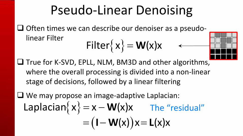
Often times we can describe our denoiser as a pseudo- linear Filter

True for K-SVD, EPLL, NLM, BM3D and other algorithms,

where the overall processing is divided into a non-linear stage of decisions, followed by a linear filtering

We may propose an image-adaptive Laplacian:

Pseudo-Linear Denoising

Filter x (x)xW

The “residual”

(x) x (x)xI W L

Laplacian x x (x)xW

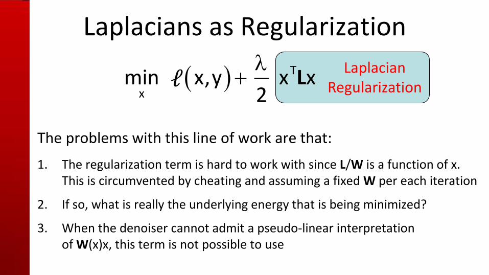
Laplacian Regularization

Laplacians as Regularization

The problems with this line of work are that:

1. The regularization term is hard to work with since L/W is a function of x. This is circumvented by cheating and assuming a fixed W per each iteration

2. If so, what is really the underlying energy that is being minimized?

3. When the denoiser cannot admit a pseudo-linear interpretation of W(x)x, this term is not possible to use

T

xmin x,y x x

2Lℓ

The Plug-and-Play-Prior (P3) Scheme

Prior-Art 2:

[Venkatakrishnan, Wohlberg & Bouman, 2013]

The P3 Scheme Use a denoiser to solve general inverse problems

Main idea: Use ADMM to minimize the MAP energy

The ADMM translates this problem (difficult to solve)

into 2 simple sub-problems:

1. Solve a linear system of equations, followed by

2. A denoising step

MAPx

x̂ min x,y x2

ℓ

P3 Shortcomings The P3 scheme is an excellent idea, as one can use ANY

denoiser, even if (⋅) is not known, but…

Parameter tuning is TOUGH when using a general denoiser This method is tightly tied to ADMM without an option for

changing this scheme CONVERGENCE ? Unclear (steady-state at best) For an arbitrarily denoiser, no underlying & consistent

COST FUNCTION

In this work we propose an alternative which is closely related to the above ideas (both Laplacian regularization and P3) which overcomes the mentioned problems: RED

RED: First Steps

Regularization by Denoising [RED]

T1x x x x

2 W

Regularization by Denoising [RED]

[Romano, Elad & Milanfar, 2016]

We suggest:

… for an arbitrary denoiser f(x)

x 0

1. x 0

2. x f x

3. Orthogonality

T1x x x f x

2

Which f(x) to Use ?

Almost any algorithm you want may be used here, from the simplest Median (see later), all the

way to the state-of-the-art CNN-like methods

We shall require f(x) to satisfy several properties as follows …

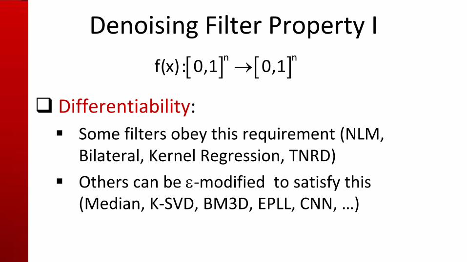
Denoising Filter Property I

Differentiability:

Some filters obey this requirement (NLM, Bilateral, Kernel Regression, TNRD)

Others can be -modified to satisfy this (Median, K-SVD, BM3D, EPLL, CNN, …)

n n

f(x): 0,1 0,1

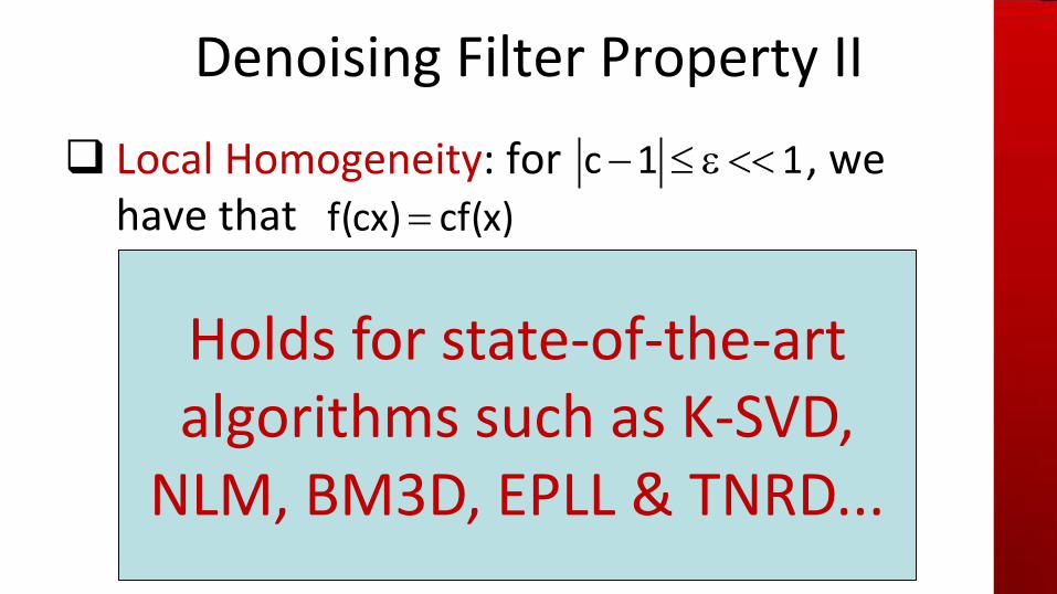
Denoising Filter Property II

Local Homogeneity: for , we have that

Filter

Filter

=

c 1 1

f(cx) cf(x)

c

c

Denoising Filter Property II

Local Homogeneity: for , we have that

Filter

Filter

=

c 1 1

f(cx) cf(x)

c

c

Holds for state-of-the-art algorithms such as K-SVD,

NLM, BM3D, EPLL & TNRD...

Implication (1)

Directional Derivative:

Homogeneity

x

0

f(x d) f(x)f x d lim

x

0

f(x x) f(x)f x x lim

0

(1 )f(x) f(x)lim f(x)

d x

Looks Familiar ?

n×n Matrix

This is much more general than and applies to any denoiser satisfying the above conditions

We got the property xf x x f(x)

f(x) (x)xW

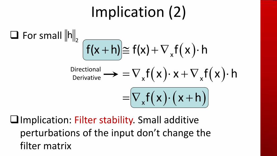
Implication (2)

For small

Implication: Filter stability. Small additive

perturbations of the input don’t change the filter matrix

Directional Derivative

xf(x h) f(x) f x h

x xf x x f x h

xf x x h

2h

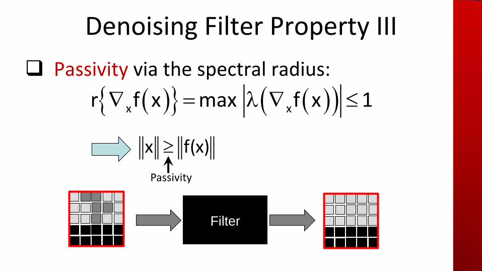
Denoising Filter Property III

Passivity via the spectral radius:

Filter

x xr f x max f x 1

Passivity

x f(x)

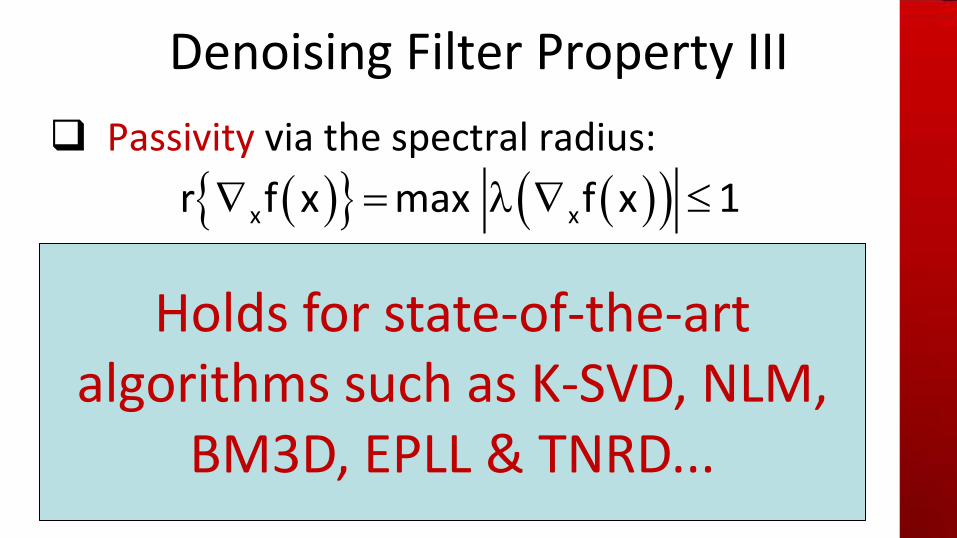
Denoising Filter Property III

Passivity via the spectral radius:

Filter

x xr f x max f x 1

x xx r f x x f x x f(x)Holds for state-of-the-art

algorithms such as K-SVD, NLM, BM3D, EPLL & TNRD...

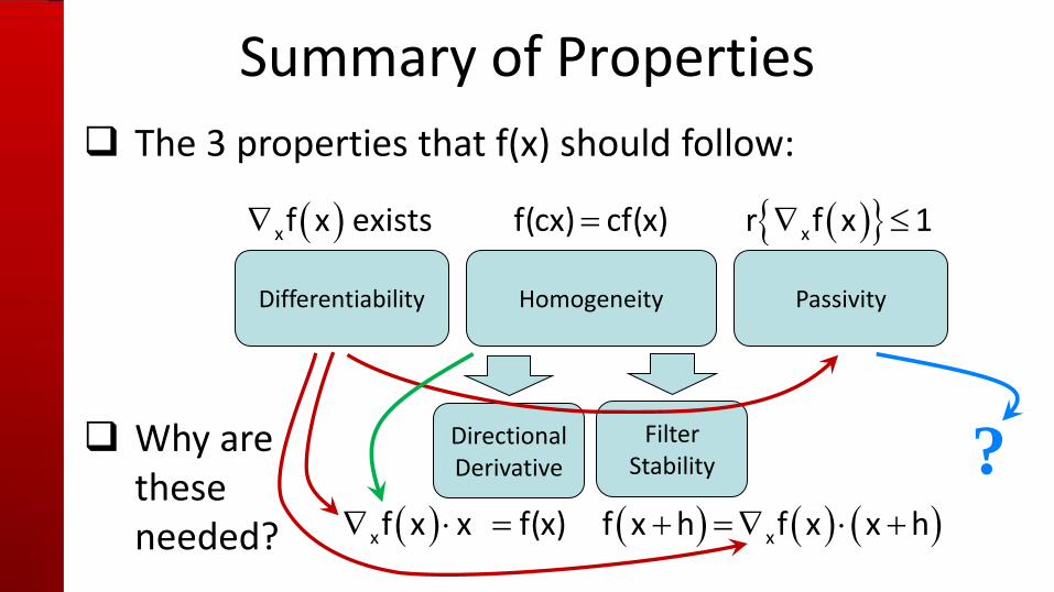
Summary of Properties

The 3 properties that f(x) should follow:

Why are these needed?

Differentiability Homogeneity Passivity

xf x exists f(cx) cf(x) xr f x 1

Directional Derivative

Filter Stability

xf x h f x x h xf x x f(x)

?

RED: Advancing

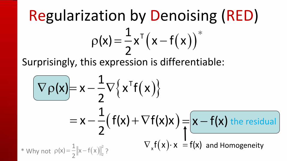
Regularization by Denoising (RED)

Surprisingly, this expression is differentiable:

T1(x) x x f x

2

T1(x) x x f x

2

1

x f(x) f(x)x2

x f(x)

xf x x f(x)

the residual

*

2

2

1(x) x f x

2* Why not ?

and Homogeneity

Passivity guarantees positive definiteness of the Hessian and hence convexity

Regularization by Denoising (RED)

T1(x) x x f x

2

(x) x f x

x(x) f xI

xr f x 1

Relying on the differentiability

≽ 0

Regularization L2-based Data Fidelity

This energy-function is convex

Any reasonable optimization algorithm will get to the global minimum if applied correctly

RED for Linear Inverse Problems

2 T

2x

1min x y x x f x

2 2

H

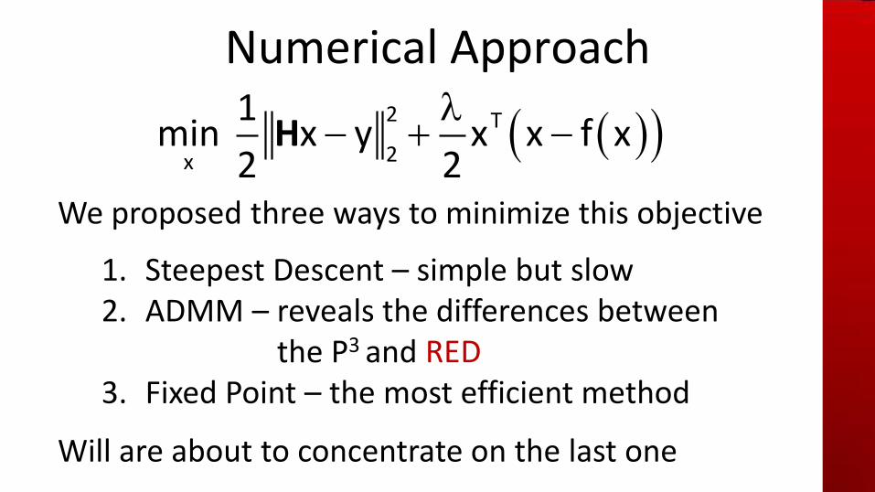
Numerical Approach

We proposed three ways to minimize this objective

1. Steepest Descent – simple but slow 2. ADMM – reveals the differences between

the P3 and RED 3. Fixed Point – the most efficient method

Will are about to concentrate on the last one

2 T

2x

1min x y x x f x

2 2

H

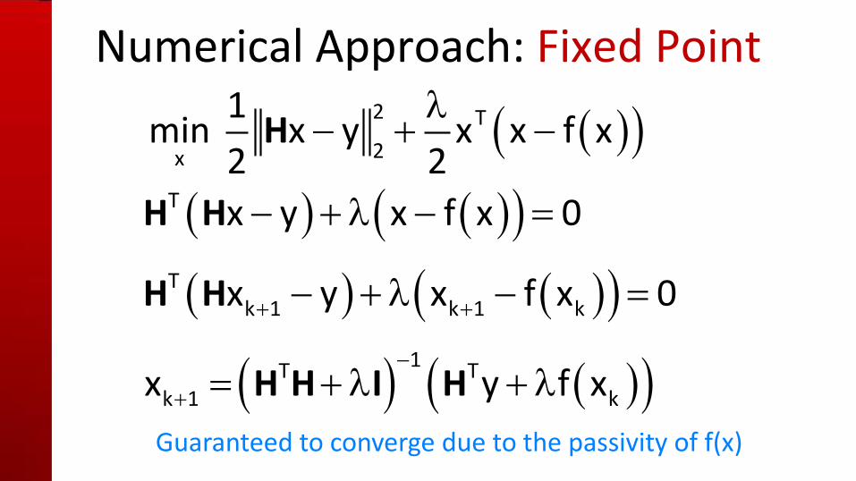
Numerical Approach: Fixed Point

Guaranteed to converge due to the passivity of f(x)

2 T

2x

1min x y x x f x

2 2

H

T x y x f x 0 H H

Tk 1 k 1 kx y x f x 0 H H

1T T

k 1 kx y f x

H H I H

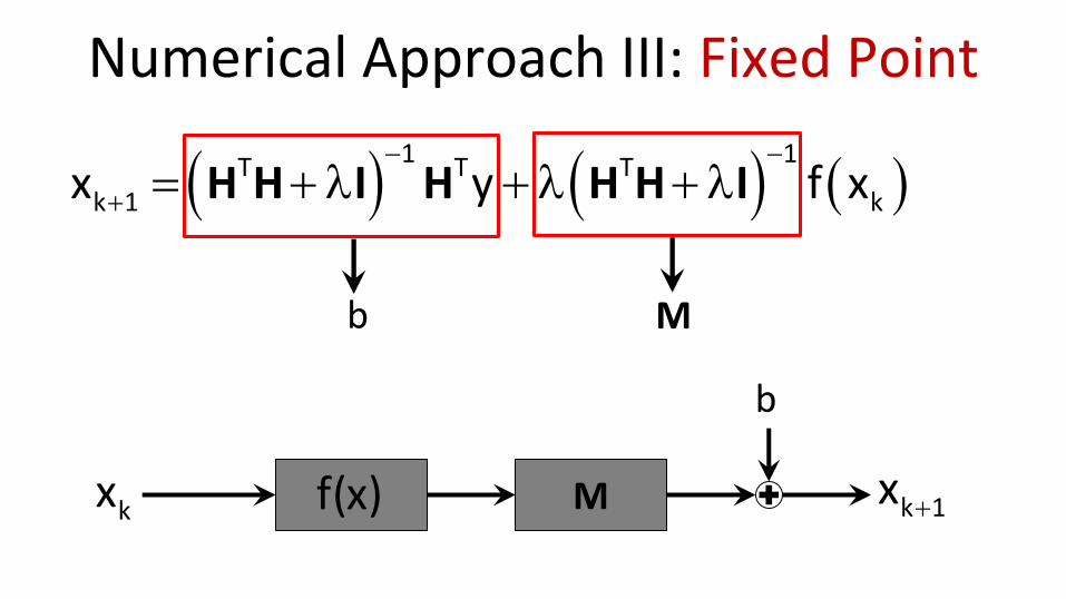
Numerical Approach III: Fixed Point

1 1T T T

k 1 kx y f x

H H I H H H I

M b

b

f(x) k 1x kx M

A connection to CNN

While CNN use a trivial and weak non-linearity f(●), we propose a very aggressive and image-aware denoiser

Our scheme is guaranteed to minimize a clear and relevant objective function

f(x) M f(x) M k 1x kxk 1x

M f(x)k 1z kz

M f(x)k 1z

k 1 kz f z b M

k 1z kz

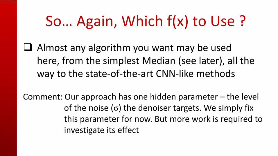
So… Again, Which f(x) to Use ?

Almost any algorithm you want may be used here, from the simplest Median (see later), all the way to the state-of-the-art CNN-like methods

Comment: Our approach has one hidden parameter – the level

of the noise (σ) the denoiser targets. We simply fix this parameter for now. But more work is required to investigate its effect

RED in Practice

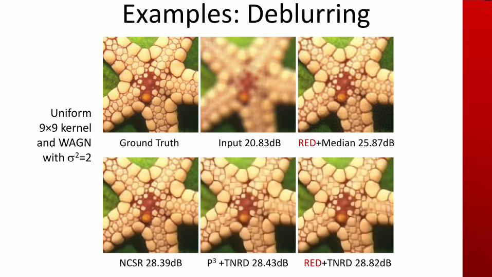
Examples: Deblurring

Uniform 9×9 kernel and WAGN

with 2=2

Ground Truth Input 20.83dB RED+Median 25.87dB

NCSR 28.39dB P3 +TNRD 28.43dB RED+TNRD 28.82dB

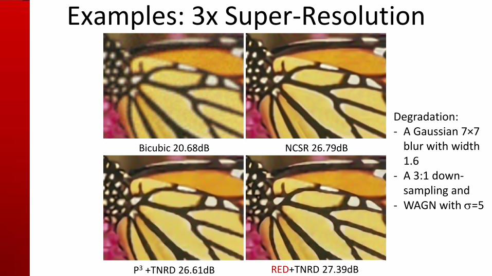
Examples: 3x Super-Resolution

Degradation: - A Gaussian 7×7

blur with width 1.6

- A 3:1 down-sampling and

- WAGN with =5

Bicubic 20.68dB NCSR 26.79dB

P3 +TNRD 26.61dB RED+TNRD 27.39dB

Sensitivity to Parameters

RED versus P3 P3: Sensitivity to parameter changes in the ADMM

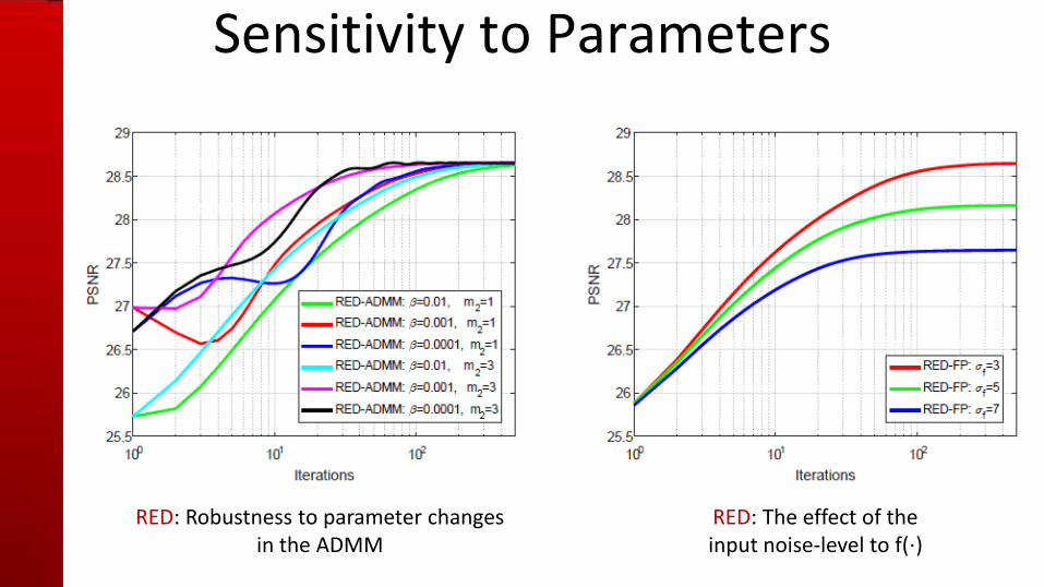
Sensitivity to Parameters

RED: Robustness to parameter changes in the ADMM

RED: The effect of the input noise-level to f(⋅)

Conclusions

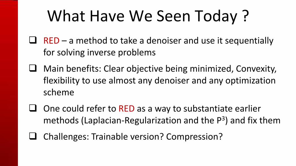
What Have We Seen Today ?

RED – a method to take a denoiser and use it sequentially for solving inverse problems

Main benefits: Clear objective being minimized, Convexity, flexibility to use almost any denoiser and any optimization scheme

One could refer to RED as a way to substantiate earlier methods (Laplacian-Regularization and the P3) and fix them

Challenges: Trainable version? Compression?

1. “Regularization by Denoising”, Y. Romano, M. Elad, and P. Milanfar, To appear, SIAM J. on Imaging Science.

2. “A Tour of Modern Image Filtering”, P. Milanfar, IEEE Signal Processing Magazine, no. 30, pp. 106–128, Jan. 2013

3. “A General Framework for Regularized, Similarity-based Image Restoration”, A. Kheradmand, and P. Milanfar, IEEE Trans on Image Processing, vol. 23, no. 12, Dec. 2014

4. “Boosting of Image Denoising Algorithms”, Y. Romano, M. Elad, SIAM J. on Image Science, vol. 8, no. 2, 2015

5. “How to SAIF-ly Improve Denoising Performance”, H. Talebi , X. Zhu, P. Milanfar, IEEE Trans. On Image Proc., vol. 22, no. 4, 2013

6. “Plug-and-Play Priors for Model-Based Reconstruction”, S.V. Venkatakakrishnan, C.A. Bouman, B. Wohlberg, GlobalSIP, 2013

7. “BM3D-AMP: A New Image Recovery Algorithm Based on BM3D Denoising”, C.A. Metzler, A. Maleki, and R.G. Baraniuk, ICIP 2015

8. “Is Denoising Dead?”, P. Chatterjee, P. Milanfar, IEEE Trans. On Image Proc., vol. 19, no. 4, 2010

10. “Symmetrizing Smoothing Filters”, P. Milanfar, SIAM Journal on Imaging Sciences, Vol. 6, No. 1, pp. 263–284

11. “What Regularized Auto-Encoders Learn from The Data-Generating Distribution”, G. Alain, and Y. Bengio, JMLR, vol.15, 2014,

12. “Representation Learning: A Review and New Perspectives”, Y. Bengio, A. Courville, and P. Vincent, IEEE Trans. on Pattern Analysis and Machine Intelligence, vol. 35, no. 8, Aug. 2013

Relevant Reading

Thank You