the local environmental consequences of coal …economics.ucdavis.edu/events/papers/112jha.pdfthe...

The Local Environmental Consequences of Coal

Procurement at U.S. Power Plants

Akshaya Jha and Nick Muller∗

October 3, 2016

Abstract

There are known to be significant environmental costs associated with burningcoal in order to generate electricity. However, there are also sizable local envi-ronmental health costs associated with power plants’ coal purchase and storagebehavior. We find that a 10% increase in coal stockpiles (number of deliveries) isassociated with a 0.02% (0.07%) increase in the concentration of fine particulateson average. Local populations exposed to these fine particulates (PM2.5) haveincreased risk of lung and heart conditions. Translating the increase in PM2.5 as-sociated with plants’ coal procurement behavior into mortality risk and monetizingthis mortality risk, we calculate local environmental costs between $0.004-$0.02 perKWh. Finally, we show that the average increase in mortality rates associated withan increase in PM2.5 are substantially higher when we instrument using coal stock-piles and number of deliveries relative to OLS specifications; this result providesboth a new identification strategy for the link between mortality rates and PM2.5

as well as further empirical evidence of the link between PM2.5 and plants’ coalprocurement behavior.

∗Akshaya Jha: H. John Heinz III College, Carnegie Mellon University, 4800 Forbes Avenue,Pittsburgh, PA 15213. Email: [email protected]. Nicholas Muller: Department ofEconomics, Middlebury College and NBER, 303 College Street, Middlebury, VT 05753. Email:[email protected].

1

1 Introduction

There is significant concern regarding the environmental costs associated with coal-fired

electricity generation in the United States. The vast majority of this concern focuses

on the global and local pollutants emitted when coal is burned to produce electricity.1

Our paper instead examines the environmental consequences of the input coal purchase

and storage behavior of U.S. power plants. The paper has three components. First, we

estimate the extent to which increases in coal stockpiles and coal deliveries are associ-

ated with increases in the locally-monitored concentration of fine particulates (termed

PM2.5).2 Local populations exposed to higher PM2.5 concentration levels have increased

risk of lung and heart conditions; we map increases in PM2.5 associated with increases

in coal stockpiles (coal deliveries) into mortality risk and ultimately a dollar-per-KWh

social cost of coal stored (delivered). Finally, we test whether mortality rates are caused

by exposure to PM2.5 using the level of coal stockpiles held and the number of coal

deliveries received by nearby power plants as instruments.

We consider monthly average PM2.5 concentration levels at roughly 1,000 monitored

sites across the United States from 2002-2012. These data are collected from the Air

Quality System (AQS) database maintained by the Environmental Protection Agency

(EPA). Our primary variables of interest (coal stockpiles and number of deliveries) come

from monthly, plant-level data on coal purchases and stockpiles provided by the Energy

Information Administration (EIA). We report results considering all coal-fired power

plants within 100 miles of each air quality monitor unless otherwise specified; we also

consider specifications with 25, 50, and 200 mile bandwidths between air quality monitor

and plants. We additionally merge in monthly, meteorological data collected by roughly

1,600 monitors across the United States given that wind speed and direction, as well as

temperature and precipitation, are important determinants of the extent to which coal

stockpiles and deliveries generate PM2.5. These data are maintained by the National

Climatic Data Center (NCDC). We find that a 10% increase in coal stockpiles (number of

deliveries) is associated with a 0.02% (0.07%) increase in PM2.5 concentration on average,

1See NRC (2010) for a comprehensive report on the environmental externalities associated with energyuse.

2Jaffe et al. (2015) studies the emissions of diesel particulate matter (DPM) and coal dust from trainsin the Columbia River Gorge in Washington State; they find that passage of a diesel powered open-topcoal train result in nearly twice as much respirable PM2.5 compared to passage of a diesel-poweredfreight train.

2

controlling for a wide array of other potential determinants of PM2.5 concentration levels

(described in Section 3).

We use a peer-reviewed concentration-response function (Krewski et al., 2009) to map

increases in PM2.5 to mortality risk; we consider the Value of a Statistical Life (VSL)

measure to monetize this mortality risk in 2013 dollars.3 We estimate that health costs are

roughly $12.54 ($7.52) per ton of coal stockpiled (delivered). These local environmental

costs are sizable given that U.S. coal-fired power plants pay roughly $48 per ton for coal

on average. However, if we translate tons of coal to KWh of electricity, our health costs

amount to roughly $0.004-$0.02 per KWh; our environmental health cost estimates for

coal purchased and stored are an order of magnitude lower than the local environmental

health costs typically estimated for coal burned. Summarizing, our empirical estimates of

the local environmental damages associated with purchasing and storing coal are sizable,

but not unreasonably so when compared to estimates of the local environmental damages

associated with burning coal.

Finally, we estimate the effect of PM2.5 concentration levels on mortality rates using

both ordinary least squares (OLS) and instrumental variables (IV) frameworks. We

consider separate regressions for mortality rates associated with different causes of death:

deaths due to the cardiovascular system, deaths due to the respiratory system, and

deaths due to the nervous system. We also consider total number of deaths of any

type and deaths due to external causes such as accidents (as a placebo test). These

county/month specific mortality rates come from the Centers for Disease Control and

Prevention (CDC Wonder, 2016). We include a range of controls in both OLS and

IV specifications as well as county/year fixed effects. We find an economically small

(and sometimes negative) association between PM2.5 and any of these mortality rates

when examining the OLS results. However, the effect of PM2.5 on mortality rates is

positive, statistically significant, and economically significant when we instrument using

the monthly level of coal stockpiles and monthly number of coal deliveries from nearby

power plants.

Previous empirical literature has found that the damages from air pollution are sig-

nificant in magnitude and that these damages are mostly due to the increased mortality

3Viscusi and Aldy (2003) reviews more than 60 studies of mortality risk premiums from ten countriesand approximately 40 studies that present estimates of injury risk premiums.

3

risk from exposure to PM2.5.4 However, recent work in economics has challenged the

causal basis for the link between exposure to PM and the adverse effects on mortality

risk reported in the epidemiological literature.5 Observational studies relating PM2.5 and

mortality rate can be confounded by increases in economic activity, changes in weather,

etc.; we demonstrate that the coal procurement behavior of U.S. power plants aids in

empirically identifying the impact of PM2.5 exposure on mortality rates. We thus provide

empirical evidence on the link between PM2.5 exposure and mortality rates using a novel

identification strategy as well as provide further empirical evidence that there’s a link

between PM2.5 concentration levels and plants’ coal procurement behavior.

The remainder of the paper proceeds as follows. In Section 2, we elaborate on the

physical process underlying how plants’ coal purchase and storage behavior can result

in higher PM2.5 concentration levels. Section 3 lists the data sources as well as the

methodology used to estimate the relationship between plants’ coal procurement behavior

and PM2.5 concentration levels, while Section 4 presents the empirical results showing

that increases in coal purchase and storage behavior correspond to increases in PM2.5

concentration levels. In Section 5, we quantify the local environmental health costs due to

the PM2.5 increases associated with plants’ coal procurement behavior. We describe our

instrumental variables approach for identifying the effect of PM2.5 concentration levels

on mortality rates in Section 6. Finally, we conclude in Section 7.

2 Economic and Environmental Background

2.1 Input Coal Procurement

Coal-fired power plants burn coal in order to heat water into steam that drives the

turbines used to generate electricity.6 These plants purchase the majority of their input

coal from long-term contracts with coal suppliers, purchasing the remainder from spot

markets. They also store large quantities of coal on-site to hedge against coal price

4This empirical literature includes NRC (2010), of Air and Radiation: Office of Policy in Washington(2010), Muller, Mendelsohn and Nordhaus (2011), and Muller (2014).

5This work includes (among others) Currie, Neidell et al. (2005), Currie, Neidell and Schmieder(2009), and Chay and Greenstone (2003).

6See http://www.duke-energy.com/about-energy/generating-electricity/coal-fired-how.asp for a shortdescription of this process.

4

http://www.duke-energy.com/about-energy/generating-electricity/coal-fired-how.asp

and supply risks; these coal inventories are very rarely resold in practice.7 Coal is not

homogeneous; coal mined from different regions of the United States differs in heat

content, sulfur content, ash content, distance from mine to plant, etc. Coal-fired power

plants primarily value the heat content of coal; burning a ton of coal with a higher

heat content generates a larger amount of output electricity. Sulfur and ash content are

important mainly for their environmental impacts. Finally, roughly 67 percent of coal is

transported via rail. The remaining coal is shipped via barge (12%), trucks (10%) and

various other modes used primarily for short distances (ex: conveyors, pipelines, etc.).8

The local environmental costs of coal delivered from the mine to the power plant can

differ significantly based on the mode of transportation utilized.

2.2 Environmental Impacts of U.S Coal-fired Generation

It is well-known that direct emissions of NOx, SO2, and PM2.5 are associated with

elevated mortality risk among exposed populations. Earlier work has shown that U.S.

coal-fired power plants emit significant levels of NOx, SO2, and PM2.5 when burning

coal; these emissions caused approximately 27,000 deaths in the U.S. in 1999. Emissions-

induced deaths resulting from power plants burning coal fell to roughly 9,500 in 2011 due

to differences in plants’ fuel choice and the increased prevalence of scrubbing technology

(Muller, 2014).

While the environmental costs associated with burning coal are well-documented

(NRC and NAS, 2010), this paper explores the local environmental costs associated

with emissions from coal stockpiles and coal deliveries. We posit two mechanisms for

emissions from coal stockpiles. The first is wind erosion. Wind blowing over uncovered

coal stockpiles entrains fine particulates; these passive, or fugitive, dust emissions become

a constituent of ambient PM2.5. Second, coal stockpiles emit volatile gases. Specifically,

coal in open stockpiles undergoes oxidation, which releases a set of pollutants including

hydrocarbons and sulphuric gases (Zhang, 2013). The gases result in the formation of

secondary organic PM2.5 that is a constituent of the ambient PM2.5 collected at monitor-

7This lack of resale is due primarily to the fact that the coal transportation infrastructure is designedto bring coal to power plants rather than away from them; therefore, coal becomes very costly to resellonce it’s in the stockpile.

8These statistics are for the year 2013 and come from EIA’s “Today In Energy”http://www.eia.gov/todayinenergy/detail.cfm?id=16651.

5

http://www.eia.gov/todayinenergy/detail.cfm?id=16651

ing stations. Coal deliveries typically arrive by train; the coal carried by these trains are

typically in uncovered freight cars. Thus, we expect coal deliveries to result in increased

PM2.5 levels both due to wind erosion (dust entrainment) and gaseous discharge. Ad-

ditionally, coal trains run on diesel fuel; burning diesel is also associated with increased

PM2.5 concentration levels. Thus, the burning of diesel is another factor determining the

local environmental costs from coal deliveries.

Our empirical strategy does not distinguish between the two types of passive emissions

(dust entrainment and gaseous discharges); PM2.5 emissions resulting from both of these

mechanisms increase mortality rates in local populations and thus contribute to local

environmental health costs. Similarly, we do not disentangle how much of the PM2.5

increase from coal deliveries comes from passive emissions from coal versus emissions

from burning diesel, as both of the factors contribute to the local environmental costs

associated with transporting coal. However, our empirical strategy does control for the

direct emissions which result from burning coal, as we focus in this paper on the local

environmental costs associated with purchasing and storing coal.

3 Local Environmental Impacts of Coal Procure-

ment: Data and Methodology

This section describes the data used to estimate the association between plant-level coal

procurement behavior (coal stockpiles and number of deliveries) and PM2.5 concentra-

tions at nearby air quality monitors. We also present the empirical framework used to

measure this association, which includes specifying our set of controls for alternative

sources of PM2.5 (ex: burning coal) as well as other factors that increase or decrease

PM2.5 for a given set of sources (ex: wind speed, wind direction, and precipitation).

3.1 Data Sources

We utilize monthly, plant-level data from 2002-2012 on end-of-month fuel inventories and

fuel purchases from the Energy Information Administration (EIA).9 For plants’ coal pur-

9The data regarding fuel inventories for 2002-2012 are confidential; we obtained a research contractfrom the EIA in order to use these restricted-access data.

6

chases, we have order-level data on the month of purchase, quantity purchased, delivered

price, heat content, sulfur content, ash content, origin of coal, and whether the order

came from a long-term contract or the spot market. Finally, we only consider electricity

generation plants whose “primary business purpose is the sale of electricity to the pub-

lic”10; this excludes plants that also sell significant quantities of heat (“combined heat

and power plants”) as well as commercial and industrial plants that generate electricity

for their own use.

We also use the Air Quality System (AQS) data provided by the Environmental

Protection Agency (EPA). This publicly available database includes hourly readings of

ambient PM2.5 concentrations at roughly 1,000 monitored sites across the contiguous U.S.

We aggregate these data to monthly average PM2.5 levels for each air quality monitor

for the sample period 2002-2012.

Our meteorological controls come from the quality controlled local climatological

data (QCLCD) collected by the National Climatic Data Center (NCDC); these data

include hourly wind speed and direction, dry bulb temperature, wet bulb temperature,

dew-point temperature, relative humidity, station pressure, and precipitation at approx-

imately 1,600 U.S. locations. Wind speed is of primary importance to quantifying the

local environmental costs associated with coal procurement as wind blowing over coal

stockpiles and coal deliveries generates PM2.5. We aggregate these data to the meteoro-

logical monitor/month-of-sample level by taking wind speed weighted averages of wind

direction, dry bulb temperature, wet bulb temperature, dew-point temperature, relative

humidity, and station pressure; the results presented below differ very little if we instead

take un-weighted averages. We also control for the (5, 10, 20, 30, 40, 50, 60, 70, 80,

90, 95) hourly percentiles of wind speed, calculated over all hours-of-sample for each

meteorological monitor/month-of-sample.

Finally, we control for a variety of other factors that can affect the PM2.5 concen-

tration reading at an air quality monitor in each month. First, the EPA’s Continuous

Monitoring Emissions System (CEMS) collects hourly data for each plant on SO2, CO2,

and NOx emissions (in tons) resulting from coal burned; we sum these hourly data to

the monthly level and control for total SO2, CO2, and NOx emissions for each plant in

each month-of-sample. We also control for the total monthly quantity of coal purchased

10This quotation is from the EIA Form 923 data dictionary.

7

by each plant as well as the total monthly electricity generation produced by each plant;

both variables come from EIA data.

The AQS database provides the latitude and longitude for each air quality monitor,

the NCDC database provides the latitude and longitude (as well as wind direction in each

month-of-sample) for each meteorological monitor, and the EPA eGrid database provides

the latitude and longitude for each coal-fired power plant. We use these variables in order

to merge air quality monitors to coal-fired power plants and meteorological monitors.

3.2 Data Merge

We merge each air quality monitor i to meteorological monitors and coal-fired power

plants as follows:

1. For each month-of-sample, we find all meteorological monitors within M miles of

the air quality monitor i. We take a weighted average of the meteorological data

(ex: wind speed, wind direction, etc.) across these meteorological monitors for each

air quality monitor i, where we weight by the inverse of the distance between the

air quality monitor and the meteorological monitor.11

2. We consider all coal-fired power plants within M miles of air quality monitor i.

Thus, our unit of observation is an air quality monitor/power plant for each month-of-

sample, emphasizing that each air quality monitor can be associated with multiple power

plants for a given month-of-sample. We examine how the effect of coal stockpiles and

number of deliveries on PM2.5 concentration levels varies by distance between air quality

monitor and power plant (i.e: considering M = (25, 50, 100, 200) miles), the relative wind

direction between air quality monitor and power plants, as well as other factors such as

wind speed, temperature, humidity, etc. For example, we hypothesize that an air quality

monitor downwind of coal-fired power plants picks up higher levels of PM2.5 relative to

an air quality monitor upwind of these coal-fired power plants. We provide further detail

on our data sources as well as data construction in Appendix Section B.

11Our empirical results do not differ substantially if we instead take an un-weighted average of themeteorological data.

8

3.3 Empirical Framework

We are interested in estimating the effect of coal stockpiles held by coal-fired power

plants on local PM2.5 concentration levels. We consider two specifications: “Log-Log”

and “Levels-Levels”. Our Log-Log specification for how coal stockpiles impact PM2.5

levels is:

log(PM2.5i,t + 1) = αc,t + θi,p + log(CSp,t)γi,p + log(

Pi,t∑k=1,k 6=p

CSk,t)ψ +Xi,p,tβ + εi,p,t (1)

where a unit of observation is an air quality monitor i and coal-fired power plant p

in month-of-sample t. Pi,t is the number of coal-fired power plants merged with each

air quality monitor i in each month t. We control for the total level of coal stockpiles

across all plants k 6= p so that the log(CSp,t) term doesn’t capture positive correlations

in stockpile increases across plants; for example, if a one ton increase in coal stockpiles

at plant p is typically associated with a 0.5 ton increase in coal stockpiles at plant q,

we do not want to include the effects of the 0.5 ton increase at plant q on PM2.5 in

our estimate of γi,p. We also control for a wide variety of alternative factors that affect

local PM2.5 levels, such as annual sulfur and ash content of coal purchased by the plant,

monthly quantity of coal received by the plant, monthly number of coal deliveries to the

plant, the plant’s monthly total electricity generation, the plant’s monthly total SO2,

CO2, and NOx emissions from coal burned (in tons), wind speed, dry bulb temperature,

wet bulb temperature, dew-point temperature, relative humidity, station pressure, and

precipitation. Finally, we include fixed effects for county-of-air-quality-monitor/month-

of-sample (αc,t) and air quality monitor/power plant (θi,p). We report a specification

considering one overall coefficient (γi,p ≡ γ), as well as specifications allowing γi,p to vary

by wind direction, wind speed, temperature, precipitation, etc.12

Our goal is to estimate how the level of PM2.5 measured by a given air quality monitor

is affected by a one ton increase in coal stockpiles, controlling for all of the other factors

listed above. The Log-Log specification in Equation 1 implies that this partial effect is:

E[PM2.5i,t|αc,t, θp,i, Xi,p,t]

dCSp,t

= γi,pexp( ˆlog(PM2.5i,t))exp(0.5σ2)CS−1i,t

12Coal-fired power plants only stock-out in roughly 0-5% of the months-of-sample for which we observethem; thus, we drop observations with zero stockpiles. The empirical results are similar if we keep thesezero stockpile observations in the sample; for these specifications, we include log(CSp,t + 1) as well as adummy variable for coal stockpile levels greater than zero 1(CSp,t > 0) instead of log(CSp,t).

9

if we assume that εi,p,t|(X,α, θ) is independently and identically distributed

Normal(0, σ2). Unfortunately, this functional form for the partial effect is highly sen-

sitive to small levels of coal stockpiles (CSp,t); the partial effects resulting from this

calculation are highly right-skewed.

Due to this, we also estimate a Levels-Levels specification:

PM2.5i,t = αc,t + θi,p + CSp,tγi,p + (

Pi,t∑k=1,k 6=p

CSk,t)ψ +Xi,p,tβ + εi,p,t

This specification includes the same set of controls as listed above; the partial effect

associated with coal stockpiles is simply γi,p in the Levels-Levels case.

Finally, we also estimate both the Log-Log and Levels-Levels specifications replacing

coal stockpiles (CSp,t) with the number of coal deliveries (NDp,t) arriving at plant p in

month-of-sample t.13 We control for the same factors as described above, with the obvious

exception of the number of deliveries (our dependent variable). We interpret the effect

of deliveries on PM2.5i,t (γi,p) as stemming primarily from the diesel fuel being burned

by the trains rather than from the coal itself as we control for the monthly quantity of

coal delivered to the plant. For both coal stockpiles and number of deliveries, we use

the partial effects generated from the Levels-Levels specification in order to quantify the

local environmental health costs associated with coal purchase and storage behavior.

4 Local Environmental Impacts of Coal Procure-

ment: Empirical Findings

In this section, we present our regression results regarding the link between coal pur-

chase/stockpiling behavior and PM2.5 concentration levels. We estimate both Levels-

Levels and Log-Log specifications, finding from the Log-Log specifications that a 10%

increase in coal stockpiles (number of deliveries) is associated with a 0.02% (0.07%) in-

crease in PM2.5 concentration on average. As discussed in Section 2.2, PM2.5 particulates

are generated both by wind blowing over coal piles and from the volatile gases emitted

13We consider log(NDp,t + 1) for the Log-Log specifications given that there are a non-trivial numberof plant/month-of-sample observations where there are zero deliveries (i.e.: the plant did not purchasecoal in that month-of-sample).

10

by coal piles; PM2.5 particulates are also created when diesel is burned by the trains

delivering coal. We thus expect more severe increases in PM2.5 concentrations for local

populations downwind from coal piles and train deliveries (i.e.: the wind is blowing from

the coal pile to the local population). Consistent with this intuition, we estimate that

the average PM2.5 increase associated with coal purchase and storage behavior is larger

for air quality monitors that are downwind of nearby coal-fired power plants. We also

find that the average PM2.5 increase associated with coal stockpiles is lower for higher

levels of precipitation. Finally, we examine air quality monitors near coal mines, simi-

larly finding that a higher number of deliveries coming from coal mines corresponds to

an increase in average local PM2.5 concentration levels.

4.1 Overall Effect of Coal Stockpiles and Number of Deliveries

on PM2.5 Concentrations

The top panel of Table 1 displays the results of the Levels-Levels specification with the

number of coal deliveries arriving at each plant in each month-of-sample as the covariate

of interest. With the sample restricted to plants within 25 miles of each air quality

monitor, we find that an additional delivery is associated with an increase in monthly

average PM2.5 levels of 0.016 micrograms per cubic meter (ug/m3). This regression model

explains nearly 85% of the variation in ambient PM2.5 readings. When we include plants

within 50 miles of each monitor in the estimation sample, the magnitude of the effect

falls by roughly 63% to 0.006 ug/m3. Further expanding the bandwidth to 100 miles or

200 miles reduces the partial effect of the number of coal deliveries to roughly 0.004 ug/m3.

The summary statistics corresponding to all regressions discussed in this section are in

Appendix Table A.1 (25 mile bandwidth), Table A.2 (50 mile bandwidth), Table A.3

(100 mile bandwidth), and Table A.4 (200 mile bandwidth). The bottom panel of Table

1 displays the results of the Log-Log models. Across each bandwidth (25, 50, 100, and

200 miles), the estimated elasticity ranges from 0.007-0.013. The partial effect of coal

deliveries on ambient PM2.5 is significant at the 5% level for all four bandwidths.

The top panel of Table 2 reports the results from the Levels-Levels specification where

the size (in tons) of the coal stockpiles held at each power plant in each month-of-sample

is the covariate of interest. A one-ton increase in coal stockpiles increases ambient PM2.5

levels by about 1.02e-06 ug/m3 when only plants within 25 miles of a monitor are included.

11

Table 1: Overall Effect of Number of Deliveries on PM2.5 Concentration

Dependent Variable: PM2.5i,t

Dist. Bandwidth (25 Miles) (50 Miles) (100 Miles) (200 Miles)NDp,t 0.0161** 0.0061 0.0043 0.0039**

(0.0073) (0.0039) (0.0027) (0.0016)

Observations 49,543 167,627 471,410 1,418,815R-squared 0.846 0.810 0.790 0.777

Dependent Variable: log(PM2.5i,t) + 1Dist. Bandwidth (25 Miles) (50 Miles) (100 Miles) (200 Miles)log(NDp,t + 1) 0.0128*** 0.0093*** 0.0080*** 0.0072***

(0.0048) (0.0027) (0.0017) (0.0011)


Standard errors clustered by air quality monitor in parentheses

Facility Code/AQ Monitor Fixed Effects Included

AQ County/Month-of-Sample Fixed Effects Included

Sum of Deliveries from Other Plants Included

Meteorological and EPA Emissions Controls Included

Coal Quality, Quantity Received, and Thermal Generation Controls Included

*** p<0.01, ** p<0.05, * p<0.1

Our estimated partial effects for the 50, 100, and 200 mile bandwidths are roughly 15%-

32% the size of the effect for the 25 mile bandwidth. The association between coal

stockpiles and PM2.5 is statistically significant and positive for all four distance bins. The

bottom panel of Table 2 shows the estimated elasticities from the Log-Log specification

of the coal stockpile models. The elasticities range from 0.0014 (for plants within 200

miles of a monitor) up to 0.0061 (for plants within 25 miles of a monitor). As with

the Levels-Levels specification, the effect size is declining as expected for larger distance

bandwidths; the effects are precisely estimated for all four distance bins.

4.2 Coal Stockpiles and Number of Deliveries on PM2.5 Con-

centrations: By Wind Direction

In this subsection, we interact the covariate of interest (the number of deliveries in Table

3 and coal stockpiles in Table 4) with the bearing from coal-fired power plant to air

quality monitor. For example, a monitor directly downwind from a plant would have a

12

Table 2: Overall Effect of Coal Stockpiles on PM2.5 Concentration


Dist. Bandwidth (25 Miles) (50 Miles) (100 Miles) (200 Miles)CSp,t 1.02e-06*** 3.29e-07*** 1.79e-07*** 1.51e-07***

(2.06e-07) (9.26e-08) (5.48e-08) (3.84e-08)


Dependent Variable: log(PM2.5i,t) + 1Dist. Bandwidth (25 Miles) (50 Miles) (100 Miles) (200 Miles)

log(CSp,t) 0.0061** 0.0031** 0.0021** 0.0014**(0.0029) (0.0016) (0.0010) (0.0007)





Sum of Stockpiles from Other Plants Included



*** p<0.01, ** p<0.05, * p<0.1

bearing of 0◦ while a monitor directly upwind from a plant would have a bearing of 180◦.

For each plant/air quality (AQ) monitor pair, we code the AQ monitor as “downwind”

from the plant if their relative bearing is less than 90◦ and code the AQ monitor as

“upwind” from the plant if their relative bearing is greater than 90◦.

The top panel of Table 3 shows that, for the sample restricted only to plants within 25

miles of each PM2.5 monitor, the partial effect of deliveries is only statistically significant

for monitors downwind from plants. This is intuitive since coal piles generate PM2.5

particulates both by wind blowing over coal piles as well as from the volatile gases emitted

by coal piles; coal deliveries (typically by train) additionally generate PM2.5 particulates

from the fuel (typically diesel) burned to transport the coal. Thus, we should expect

more severe increases in PM2.5 concentrations for local populations downwind from coal

piles and coal deliveries. In addition, the magnitude of the effect for downwind monitors

is larger than the effect for upwind monitors for all four distance bandwidths (25, 50,

100, and 200 miles). Finally, as expected, the effect for downwind monitors is larger than

the corresponding effect reported in the top panel of Table 1 (which does not specifically

13

control for the orientation between plants and monitors) for all four distance bandwidths.

Table 3: Effect of Number of Deliveries on PM2.5 Concentration: Upwind vs.Downwind


Distance Bandwidth (25 Miles) (50 Miles) (100 Miles) (200 Miles)NDp,t×

Monitor Downwind from Plant 0.0217*** 0.0063 0.0050* 0.0050***(0.0084) (0.0044) (0.0030) (0.0019)

Monitor Upwind from Plant 0.0098 0.0059 0.0033 0.0024(0.0089) (0.0047) (0.0033) (0.0019)


Dependent Variable: log(PM2.5i,t) + 1Dist. Bandwidth (25 Miles) (50 Miles) (100 Miles) (200 Miles)log(NDp,t + 1)×

Monitor Downwind from Plant 0.0163*** 0.0106*** 0.0089*** 0.0083***(0.0049) (0.0029) (0.0019) (0.0012)

Monitor Upwind from Plant 0.0094* 0.0078*** 0.0070*** 0.0059***(0.0051) (0.0030) (0.0019) (0.0012)








*** p<0.01, ** p<0.05, * p<0.1

The bottom panel of Table 3 shows the results for the directional models expressed in

terms of elasticities. Across all bandwidths, the coefficients for deliveries to plants upwind

of the air quality monitor are significant at the 0.01 level. The elasticities range between

0.008 and 0.016, with the magnitude descending as we increase the distance bandwidth.

As with the Levels-Levels specification, we see that the PM2.5 elasticities with respect to

number of deliveries are smaller for upwind monitors relative to downwind monitors for

all four distance bandwidths. As expected, the downwind effects for number of deliveries

14

reported in Table 3 are larger than the corresponding overall estimates reported in the

bottom panel of Table 1 for all four distance bandwidths.

Table 4 displays the results for the directional models in which the size (in tonnage)

of coal stockpiles is the independent variable of interest. The interaction terms between

the (level of) coal stockpiles and the dummy variable for (relative) angles between the 0◦

to 90◦ are statistically significant across all four bandwidths. We see the same pattern

as with the number of deliveries regressions: 1) the estimated coefficients for downwind

monitors are larger than the corresponding estimates for upwind monitors across all four

distance bins, and 2) the estimated coefficients for downwind monitors are larger than

the corresponding overall estimates reported in the top panel of Table 2. These same

two findings (downwind larger than upwind and downwind larger than overall) also hold

when examining the Log-Log specifications presented in the bottom panel of Table 4.

4.3 Coal Stockpiles and Number of Deliveries on PM2.5 Con-

centrations: Interacted with Precipitation

In this subsection, we interact the covariate of interest (the number of deliveries in Table

5 and coal stockpiles in Table 6) with the logarithm of monthly average precipitation

as measured by the set of meteorological monitors within M miles of the air quality

monitor. For example, if there are four meteorological monitors within 100 miles of a

given air quality monitor (for the 100 mile bandwidth), we use the wind-speed weighted

average over both the hourly data on precipitation and over all four of these monitors

for each month-of-sample.

The top panel of Table 5 shows that an increased number of coal deliveries generates

less additional PM2.5 for higher levels of precipitation. This is intuitive, given that local

pollution levels are known to decrease with rainfall due to “wet deposition” (i.e.: PM2.5

particulates are brought from the atmosphere to the ground by rain). Thus, if burning

diesel in order to transport coal via train generates a given amount of PM2.5, less PM2.5

remains in the atmosphere for higher levels of monthly average precipitation. We interact

the logarithm of number of deliveries with monthly average precipitation in the bottom

panel of Table 5; we draw exactly the same conclusions as above using the Log-Log

specification.

15

Table 4: Effect of Coal Stockpiles on PM2.5 Concentration: Upwind vs. Downwind


Distance Bandwidth (25 Miles) (50 Miles) (100 Miles) (200 Miles)CSp,t×

Monitor Downwind from Plant 1.14e-06*** 3.58e-07*** 1.83e-07*** 1.64e-07***(2.19e-07) (1.01e-07) (5.83e-08) (4.23e-08)

Monitor Upwind from Plant 9.18e-07*** 3.05e-07*** 1.75e-07*** 1.37e-07***(2.33e-07) (1.09e-07) (6.54e-08) (4.41e-08)


Dependent Variable: log(PM2.5i,t) + 1Dist. Bandwidth (25 Miles) (50 Miles) (100 Miles) (200 Miles)log(CSp,t)×

Monitor Downwind from Plant 0.0067** 0.0033** 0.0022** 0.0016**(0.0029) (0.0016) (0.0010) (0.0007)

Monitor Upwind from Plant 0.0056* 0.0029* 0.0020* 0.0012*(0.0028) (0.0016) (0.0010) (0.0007)








*** p<0.01, ** p<0.05, * p<0.1

Table 6 displays the results interacting monthly average precipitation with coal stock-

piles. As with the number of deliveries, if a given level of coal stockpiles translates into a

given level of PM2.5, we should expect less of this PM2.5 to remain in the atmosphere for

higher levels of precipitation due to wet deposition. We find that this intuition holds for

both the top panel (Levels-Levels specification) and bottom panel (Log-Log specification)

of Table 6. Namely, we see from Table 6 that the interaction term between coal stockpiles

and monthly precipitation is statistically significant and negative across all four distance

bandwidths.

16

Table 5: Effect of Number of Deliveries on PM2.5 Concentration: Interacted withPrecipitation



Constant 0.0550*** 0.0417*** 0.0465*** 0.0388***(0.0141) (0.0074) (0.0066) (0.0046)

log(Precipitation+ 1) -0.0285*** -0.0261*** -0.0322*** -0.0262***(0.0086) (0.0048) (0.0043) (0.0030)



Constant 0.0279*** 0.0289*** 0.0316*** 0.0300***(0.0065) (0.0040) (0.0033) (0.0027)









*** p<0.01, ** p<0.05, * p<0.1

4.4 Effect of the Number of Deliveries on PM2.5 Concentrations

at Coal Mines

We also know the originating coal mine county for each coal delivery in our data-set; we

re-run our analysis by counting up the number of deliveries originating from each coal

mine county in each month-of-sample, merging each air quality monitor with coal mine

counties using the latitude and longitude of the centroid of the coal mine county.14 The

14We unfortunately do not have data on the level of coal stockpiles held at coal mines.

17

Table 6: Effect of Coal Stockpiles on PM2.5 Concentration: Interacted withPrecipitation



Constant 1.65e-06*** 6.59e-07*** 6.95e-07*** 7.02e-07***(2.59e-07) (1.27e-07) (1.04e-07) (7.74e-08)

log(Precipitation+ 1) -4.67e-07*** -2.34e-07*** -3.48e-07*** -3.61e-07***(1.29e-07) (6.75e-08) (6.18e-08) (4.62e-08)



Constant 0.0116*** 0.0100*** 0.0107*** 0.0113***(0.0030) (0.0017) (0.0012) (0.0009)









*** p<0.01, ** p<0.05, * p<0.1

bottom panel of Table 7 presents the results of this exercise for the Log-Log specification.

We find a positive and statistically significant coefficient on the logarithm of number of

deliveries for the 50, 100, and 200 mile bandwidths; however, we cannot interpret the

magnitude of the coefficients across different distance bins as we use the latitude and

longitude of the centroid of the originating coal mine county rather than the location of

the mine itself. Overall, these results indicate that coal deliveries (typically by rail) are

associated with increased PM2.5 concentrations whether coming from the mine or arriving

at the coal-fired power plant, though we see from comparing Table 7 with Table 1 that

18

the overall average effect of deliveries coming from mine counties is smaller in magnitude

relative to the overall effect of deliveries arriving at coal-fired power plants. We draw the

same qualitative conclusions when examining the Levels-Levels results displayed in the

top panel of Table 7.

Table 7: Effect of Number of Deliveries on PM2.5 Concentration: At the Coal Mine

Dependent Variable: PM2.5i,t)Dist. Bandwidth (25 Miles) (50 Miles) (100 Miles) (200 Miles)

NDp,t 0.0146 0.0013 0.0065*** 0.0084***(0.0098) (0.0062) (0.0025) (0.0023)


Dependent Variable: log(PM2.5i,t) + 1Dist. Bandwidth (25 Miles) (50 Miles) (100 Miles) (200 Miles)log(NDp,t + 1) 0.0061 0.0073*** 0.0039*** 0.0034***

(0.0079) (0.0023) (0.0009) (0.0007)





Quantity Sent Control Included

Meteorological Controls Included

*** p<0.01, ** p<0.05, * p<0.1

5 Local Environmental Health Costs of Coal Pro-

curement: Quantification

The previous section measures the effect of increases in coal stockpiles and number of coal

deliveries on local PM2.5 concentration levels. This section provides details on both the

methodology and empirical results mapping these coal procurement induced increases in

PM2.5 to mortality risk and ultimately social costs (in both dollars per ton and dollars

per KWh). Summarizing our findings, we calculate that a one ton (KWh) increase in

coal stockpiles or quantity delivered is associated with local environmental costs between

$7.50-$27 ($0.004-$0.02).

19

5.1 Mapping Partial Effects into Local Environmental Costs:

Methodology

In the previous section, we discussed how to measure the extent to which fugitive and

gaseous emissions from coal stockpiles, as well as the emissions from burning diesel as-

sociated with coal deliveries, have an effect on ambient PM2.5 levels. We estimate the

impact that such emissions have on human health in this section. We focus exclusively

on mortality risk because prior research has shown that the majority of damage from

PM2.5 exposure (and air pollution exposure, more generally) is due to elevated mortality

risk (EPA (1999); Muller, Mendelsohn and Nordhaus (2011)). This aspect of the anal-

ysis relies on the partial effects from the Levels-Levels specification (which we denote

∆PM2.5). We use the following concentration-response relationship from Krewski et al.

(2009) in order to map these partial effects into the total number of deaths stemming

from coal procurement induced changes in PM2.5:

Mc,t = Popc,tMRc,t(1−1

exp(ρ∆PM2.5i)) (2)

where Popc,t is the population in county of monitor i, denoted c in month-of-sample

t, MRc,t is the county/month-of-sample specific mortality rate, and ρ is a statistically

estimated parameter reported by Krewski et al. (2009); The result of these calculations

is an estimate of the county/month-of-sample specific deaths due to increased PM2.5

exposure stemming from coal stockpiles (or deliveries).

In Equation 2 above, ∆PM2.5 denotes the partial effect of either coal stockpiles or

number of deliveries on ambient PM2.5 concentrations using the Levels-Levels specifica-

tion. However, we divide the partial effect from an additional delivery by the number of

tons delivered to plant p in month-of-sample t in order to derive a comparable marginal

damage figure for coal stockpiles versus quantity of coal delivered. We then average this

marginal effect over plants and months-of-sample for each air quality monitor i.

The next step is quantifying the costs (in dollars) of these deaths. We employ the

Value of a Statistical Life (VSL) methodology (Viscusi and Aldy, 2003) for this conver-

sion. We use a VSL of roughly $9.8 million based on the Regulatory Impact Analyses

(RIAs) for air pollution conducted by the USEPA. The monetary marginal damage from

emissions resulting from an additional ton stored in a coal stockpile in county of monitor

20

i, denoted c, at time t, is given by:

MDCSc,t = MCS

c,t V SL

5.2 Mapping PM2.5 Concentrations to Local Environmental

Costs: Empirical Results

We calculate the local environmental health costs associated with the partial effects re-

lating coal stockpiles/number of deliveries to PM2.5 emissions using the methodology

discussed above. We use the Levels-Levels specifications that account for the wind direc-

tion between air quality monitor and coal-fired power plant (i.e: the top panel of Table

3 for number of deliveries or the top panel of Table 4 for coal stockpiles).15 Table 8

shows the results from these social cost calculations for the median air quality monitor;

we present the median social cost rather than the average social cost as the air quality

monitor level distribution of these social costs is right-skewed. We see from this table

that the monetary damage per ton of coal delivered due to increased mortality rates is

roughly $41 when using the partial effects from the Levels-Levels regression model re-

stricting the sample to plants within 25 miles of monitors. The impact rises to $114 per

ton of coal stored when the partial effect estimated from the stockpile model (25 mile

bandwidth) is used. As a point of comparison, the average delivered price of coal is $48

per ton, demonstrating that these per-ton local environmental damages are quite large.

However, the social cost estimates are sensitive to the bandwidth; this is expected

given that the effects of coal procurement on PM2.5 differ significantly across radii. We

see that the median local environmental damage associated with a one ton increase in coal

stockpiled (delivered) drops precipitously to $27.17 ($13.09) if we consider the 50 mile

bandwidth instead of the 25 mile bandwidth. Our damage estimates drop even further

to $12.54 ($7.52) per ton stockpiled (delivered) if we consider the 100 mile bandwidth.

The cost estimates do not change appreciably when using the 200 mile models; thus, we

report the 100 mile models as our primary specification.

We see that the local environmental damages associated with storing coal are either

15Appendix Table A.7 and Table A.8 repeat this analysis using the models that do not explicitlycontrol for the direction between plants and PM monitors. The basic message from comparing TableA.7 with Table 8 as well as Table A.8 with Table 9 is that controlling for direction does not have a verylarge effect on the social cost estimates for coal stockpiles or coal deliveries.

21

larger or roughly similar to the local environmental costs of delivering coal. This may

be because coal deliveries occur roughly once a week while coal stockpiles are sitting

at the power plant throughout the month. Moreover, our estimated partial effects for

the number of deliveries are based on specifications controlling for the quantity of coal

delivered; thus, we are primarily capturing the effects of emissions from the diesel burned

by the trains delivering the coal. The overall local environmental impact of coal deliveries

including both the diesel burned as well as the passive and fugitive emissions associated

with coal are likely larger than the numbers we report in Table 8. In fact, one can add

our costs per ton from coal stockpiles and number of deliveries in order to get a back-

of-the-envelope number for the overall per-ton local costs of delivering coal; this number

for the 100 mile bandwidth is roughly $20 per ton delivered.

Our per-ton local environmental damage estimates are large given that the average

price of coal is roughly $48. However, Table 9 demonstrates that our estimates are not

unreasonably large when compared to estimates in the literature of the local environ-

mental costs associated with burning coal. Converting tons of coal burned to KWh of

electricity generated, our estimates of the per-KWh social costs associated with storing

(delivering) coal range from roughly $0.005 to $0.055 ($0.005 to $0.021). These local

environmental health cost estimates for coal purchased and stored are roughly an order

of magnitude lower than the local environmental health costs typically estimated for coal

burned. We should expect this given that burning coal emits significantly more PM2.5

relative to storing or transporting coal.

Table 8: Per-ton Social Cost Estimates from the Models that do control for Direction

(25 Miles) (50 Miles) (100 Miles) (200 Miles)CSp,t 113.80 27.17 12.54 9.41

numdelivp,t 41.38 13.09 7.52 10.36

Table 9: Per-KWh Social Cost Estimates from the Models that do control for Direction


numdelivp,t 0.0213 0.0058 0.0037 0.0048

Figure 1 is a U.S. map displaying the geographic dispersion of our air quality monitor

specific estimates of the local environmental damages from increased PM2.5 exposure

22

associated with increases in coal stockpiles. This figure indicates that local environmental

damages are higher in areas with higher populations; for example, we see particularly

high local environmental health costs associated with coal stockpiles in the Northeastern

region of the U.S. Figure 2 demonstrates directly that our estimates of the per-KWh local

environmental costs from coal stockpiling increase with total population; interestingly,

this figure also suggests a roughly linear relationship between local environmental health

costs and total population.

Figure 1: Damages Per Ton (Stockpiles) across the U.S.

6 IV Regression of PM2.5 on Mortality Rates

The previous section maps PM2.5 concentration increases associated with coal procure-

ment to mortality risk based on the concentration-response relationship reported by

Krewski et al. (2009) (an epidemiological study). This section directly quantifies the

impact of PM2.5 concentration levels on various type of mortality rates (such as deaths

related to the cardiovascular system, deaths related to the respiratory system, etc.) using

23

Figure 2: Damages Per Ton (Stockpiles) versus Total Population

0.5

11.

5St

ockp

ile D

amag

e ($

/kw

h)

0 1000000 2000000 3000000 4000000 5000000County Population

coal stockpiles and number of deliveries as an instrument for PM2.5 concentration lev-

els. We first describe the data on mortality rates used for this section. We next specify

the ordinary least squares (OLS) and instrumental variables (IV) regression frameworks

measuring the impact of PM2.5 on mortality rates due to different causes. Finally, we

present our empirical results for both OLS and IV specifications.

6.1 Data Sources For Mortality Rate Regressions

We collect monthly, county-level total number of deaths by type from the Center for

Disease Control and Prevention (CDC); these categories are deaths related to the car-

diovascular, respiratory, or nervous systems, deaths due to external causes, and total

number of deaths. We present results considering only people who are 30 years old or

older, as this is the sub-population considered in epidemiological studies such as Krewski

et al. (2009). We also provide the empirical results counting deaths of people of all ages

24

in Appendix A; these all-age results are very similar to those presented below for the

over-30 subpopulation.

We also use annual, county-level population data from the Survey of Epidemiology

and End Results (SEER) collected from the National Bureau of Economic Research

(NBER) website. We consider the annual, county-level population of people at or above

30 years old for the empirical results presented below; we use the annual, county-level

population counting people of all ages for the “all-age” mortality rate regression results

provided in Appendix A.

6.2 Empirical Framework

We estimate the following ordinary least squares (OLS) specification relating mortality

rates to local PM2.5 concentrations:

log(deathsc,tpopc,y

) = αc,y + log(PM2.5i,t + 1)γ +Xi,p,tβ + εi,p,t

where c indexes the county where air quality monitor i is located, p indexes a coal-

fired power plant, t indexes the month-of-sample, and y indexes the year-of-sample. We

include the same set of controls Xi,p,t as described in Section 3. Finally, we control for

county-year fixed effects αc,y. We estimate this OLS specification separately for each

type of mortality rate (cardiovascular, respiratory, nervous, external, and total).

In our instrumental variables (IV) specifications, we instrument for log(PM2.5i,t + 1)

with both log(CSp,t) and log(NDp,t + 1); our first-stage regression is:

log(PM2.5i,t + 1) = δc,y + log(CSp,t + 1)θ1 + log(NDp,t + 1)θ2

+Xi,p,tη + εi,p,t

As with the OLS framework, we estimate this IV specification separately for each type

of mortality rate (cardiovascular, respiratory, nervous, external, and total). We cluster

standard errors by air quality monitor. We weight both OLS and IV specifications

by county-year level population; our empirical results are qualitatively similar if we do

not weight by population. We also present IV results using only coal stockpiles as an

instrument for PM2.5 concentration levels, including the number of coal deliveries as

25

a control in both the first and second stages; our empirical findings using only coal

stockpiles as an instrument are quite similar to those presented below.

6.3 Empirical Results

We relegate the summary statistics for the empirical results in this subsection to Ap-

pendix Section A. This Appendix section also contains the empirical results from the

mortality rate regressions for the full population rather than the sub-population over 30

(see Appendix Tables A.19 through A.26); the empirical results for the full population

are quite similar to the results for the over-30 subpopulation described below. We also

obtain similar results if we only use coal stockpiles as an instrument rather than both

coal stockpiles and number of coal deliveries (see Appendix Tables A.27 through A.34).

Finally, we focus for expositional ease on the results using plants within 100 miles of the

air quality monitor; we would draw similar conclusions based on the results using the 25,

50, and 200 mile distance bandwidths instead (these results are provided in Appendix

Section A).

The top panel of Table 10 lists the empirical results when regressing mortality rate

(separately for deaths associated with the cardiovascular system, the respiratory system,

the nervous system, all people, and external causes such as accidents) on PM2.5 concen-

trations within the OLS framework described in the previous subsection. Interpreting

the first column, we find that a 10% increase in PM2.5 concentration levels corresponds

to a 0.1% increase on average in the cardiovascular mortality rate (i.e: the fraction of

the population that dies due to issues related to the cardiovascular system). We find

from Column 2 that a 10% increase in PM2.5 is associated with a 0.2% average increase

in the rate of deaths related to the respiratory system. The OLS coefficient estimates

in Columns 1 and 2 are statistically significant. However, Column 3 shows a negative

(and statistically significant) association between PM2.5 exposure and the nervous system

death rate, while the total death rate coefficient estimate (Column 4) is not statistically

significant. The death rate due to external causes (such as accidents) should not be

related to PM2.5 concentration levels; however, the OLS results in Column 6 show a

negative (and statistically significant) association between the external death rate and

PM2.5.

26

Table 10: PM2.5 on Mortality Rate: 100 Mile Bandwidth for Ages 30+

OLS SpecificationVARIABLES Cardio MR Resp. MR Nervous MR Total MR External MR

log(PM2.5 + 1) 0.0102*** 0.0226*** -0.0202*** 0.0005 -0.0169***(0.0024) (0.0037) (0.0059) (0.0018) (0.0047)

Observations 381,277 295,534 221,833 403,183 226,132R2 0.901 0.758 0.823 0.922 0.734

IV SpecificationVARIABLES Cardio MR Resp. MR Nervous MR Total MR External MR

log(PM2.5 + 1) 0.202*** 0.184** 0.261*** 0.184*** -0.0373(0.0390) (0.0826) (0.0664) (0.0328) (0.0609)

Observations 366,338 283,632 212,573 386,973 217,146R2 0.880 0.746 0.798 0.890 0.736


County of AQ Monitor/Year-of-Sample Fixed Effects Included



*** p<0.01, ** p<0.05, * p<0.1

In contrast, the bottom panel of Table 10 provides the empirical results relating PM2.5

concentration levels to mortality rates for the IV specification. As with the OLS results,

we find a positive (and statistically significant) link between PM2.5 concentration levels

and both the cardiovascular and respiratory death rates (Columns 1 and 2 of the bottom

panel of Table 10). However, the estimated coefficients in Columns 1 and 2 are much

larger for the IV specification relative to the OLS specification; the IV findings indicate

that a 10% increase in PM2.5 concentration levels results in a roughly 2% (1.8%) average

increase in the cardiovascular (respiratory) mortality rate. Moreover, the IV coefficient

estimates in Columns 3 and 4 are positive and statistically significant as expected; we

find a positive link between PM2.5 exposure and both nervous system mortality rates

as well as total mortality rates. Using the IV framework, we do not see a statistically

significant relationship between the external death rate and PM2.5 exposure in Column 5;

this finding is consistent with the intuition that the probability of death due to external

causes such as accidents should not change appreciably with PM2.5 concentration levels.

27

Thus, this lack of a relationship between PM2.5 and the external death rate provides

evidence that we are not capturing some other source of variation that simultaneously

induces increases in PM2.5 concentration levels and mortality rates.

We compare our mortality estimates to those in the literature by focusing on the

overall total mortality rate for the subsample of people over 30 years old because these

estimates are directly comparable to the numbers utilized by the USEPA in its regulatory

impact analyses for PM2.5. In particular, the USEPA typically uses the association

between PM2.5 levels and overall, post-30 mortality rates reported by Lepeule et al.

(2012) and Krewski et al. (2009). However, these studies report semi-elasticities so we

perform some back-of-the-envelope calculations to compare our numbers to the numbers

found in their studies.

Lepeule et al. (2012) report that a 1 ug/m3 increase in PM2.5 is associated with a

1.4% increase in overall, post-30 mortality rates. The annual mean PM2.5 reading in

2014 was 8.4 ug/m3. At this mean PM2.5 level, a 1 ug/m3 increase in PM2.5, amounts to

a 11.9% increase in PM2.5 levels. According to the coefficient reported by Lepeule et al.

(2012) this suggests an elasticity of 0.0140.119

= 0.12. Our estimated elasticities for the total

mortality rates of people over 30 years old from the IV specifications range between 0.09

and 0.20 depending on the distance bandwidth considered. Thus, the estimate of the

all-cause, post-30 mortality elasticity with respect to PM2.5 implied by Lepeule et al.

(2012) (which is 0.12) falls into our range of estimated elasticities (which is 0.11-0.20),

though our elasticity estimates are slightly larger than 0.12 for the 50, 100 and 200 mile

bandwidth specifications.

Importantly, PM2.5 levels have fallen since the Lepeule et al. (2012) study was pub-

lished. For example, the annual average PM2.5 level was 12.47 ug/m3 in 2008. Thus, a

1 unit change in PM2.5 from the 2008 annual average level implies an elasticity of 0.18;

this lies squarely in our estimated range of elasticities. If we instead do the same calcula-

tion using the results from Krewski et al. (2009), we obtain an elasticity of 0.0060.119

= 0.05.

Summarizing, our IV estimate of the elasticity all-cause, post-30 mortality elasticity with

respect to PM2.5 is quite similar to the Lepeule et al. (2012) estimate but larger than

the Krewski et al. (2009) estimate.

28

7 Conclusion

The environmental impacts of burning coal to generate electricity are well-documented;

in this paper, we demonstrate that there are additional local environmental health costs

associated with the PM2.5 particulates generated both by wind blowing over (unburned)

coal piles, volatile gases emitted by coal piles, as well as the diesel burned when trains

deliver coal. We find that a 10% increase in coal stockpiles (number of deliveries) is

associated with a 0.02% (0.07%) increase in PM2.5 concentration on average; these PM2.5

concentration increases are most severe for local populations downwind from coal-fired

power plants. We next use a peer-reviewed concentration-response function to map

increases in PM2.5 to mortality risk and the Value of a Statistical Life (VSL) approach

to monetize these risks. Our results indicate that health costs are roughly $12.54 ($7.52)

per ton of coal stockpiled (delivered). Given that U.S. coal-fired power plants on average

pay roughly $48 per ton for coal, these local environmental costs are sizable. However,

they are not unreasonably large, given that our estimates of the per-KWh local damages

(between $0.004-$0.02 per KWh) associated with delivering and storing coal are roughly

an order of magnitude smaller than the local environmental damages of burning coal

found in the literature.

Finally, we directly estimate the effect of PM2.5 on mortality rates by type (i.e.:

cardiovascular deaths, respiratory deaths, nervous system deaths, etc.). We find that

ordinary least squares (OLS) regressions of PM2.5 exposure on mortality rates yield eco-

nomically small, sometimes negative, coefficient estimates; in contrast, if we instrument

for PM2.5 with coal stockpiles and number of coal deliveries, we see sizable positive (and

statistically significant) effects of PM2.5 exposure on mortality rates. Our estimates using

this new identification strategy are roughly in line with those found in the epidemiolog-

ical literature. The USEPA, among others, uses the mortality effects estimated in this

epidemiological literature in order to assess the environmental costs of PM2.5 exposure;

our IV estimates provide evidence that studies using this epidemiological literature are

not significantly over-estimating or under-estimating the effects of PM2.5 on mortality

rates.

Though there are economic costs associated with covering coal stockpiles or rail cars

containing coal, these costs are almost certainly small when compared to the environ-

mental costs incurred by populations local to coal-fired power plants. Moreover, a policy

29

requiring that coal stored or delivered is covered does not require significant co-ordination

across jurisdictions as these environmental costs are incurred local to the jurisdiction

where the activity is taking place (i.e.: they are incurred near coal-fired power plants).

This stands in direct contrast to proposed policy interventions for global pollutants such

as the CO2 emissions generated when coal is burned. Finally, the local environmental

health costs associated with coal piles applies more broadly than our examination of

U.S. coal-fired power plants; for example, terminals exporting U.S. coal, railroads used

to transport coal, and coal mines may also be associated with increased PM2.5 exposure.

We plan to explore in future research whether local populations near these coal terminals,

mines, etc. are similarly affected by increased PM2.5 exposure, especially those working

closely with coal (for example, coal miners).

References

Chay, Kenneth Y, and Michael Greenstone. 2003. “The Impact of Air Pollution

on Infant Mortality: Evidence from Geographic Variation in Pollution Shocks Induced

by a Recession.” The Quarterly Journal of Economics, 1121–1167.

Currie, Janet, Matthew Neidell, and Johannes F Schmieder. 2009. “Air pollution

and infant health: Lessons from New Jersey.” Journal of health economics, 28(3): 688–

703.

Currie, Janet, Matthew Neidell, et al. 2005. “Air Pollution and Infant Health:

What Can We Learn from California’s Recent Experience?” The Quarterly Journal of

Economics, 120(3): 1003–1030.

EPA, S. 1999. “The Benefits and Costs of the Clean Air Act: 1990 to 2010.” EPA-410-

R99-001. Washington, DC: US Environmental Protection Agency, Office of Air and

Radiation.

Jaffe, Daniel, Justin Putz, Greg Hof, Gordon Hof, Jonathan Hee, Dee Ann

Lommers-Johnson, Francisco Gabela, Juliane L Fry, Benjamin Ayres,

Makoto Kelp, et al. 2015. “Diesel particulate matter and coal dust from trains in

the Columbia River Gorge, Washington State, USA.” Atmospheric Pollution Research,

6(6): 946–952.

30

Krewski, Daniel, Michael Jerrett, Richard T Burnett, Renjun Ma, Ed-

ward Hughes, Yuanli Shi, Michelle C Turner, C Arden Pope III, George

Thurston, Eugenia E Calle, et al. 2009. Extended follow-up and spatial analysis

of the American Cancer Society study linking particulate air pollution and mortality.

Health Effects Institute Boston, MA.

Lepeule, Johanna, Francine Laden, Douglas Dockery, and Joel Schwartz. 2012.

“Chronic exposure to fine particles and mortality: an extended follow-up of the Harvard

Six Cities study from 1974 to 2009.” Environmental health perspectives, 120(7): 965.

Muller, Nicholas Z. 2014. “Boosting GDP growth by accounting for the environment.”

Science, 345(6199): 873–874.

Muller, Nicholas Z, Robert Mendelsohn, and William Nordhaus. 2011. “En-

vironmental accounting for pollution in the United States economy.” The American

Economic Review, 101(5): 1649–1675.

NRC and NAS. 2010. “Hidden Costs of Energy: Unpriced Consequences of En-

ergy Production and Use.” National Research Council (US). Committee on Health·Environmental· and Other External Costs and Benefits of Energy Production and

Consumption. National Academies Press.

NRC, NAS. 2010. Hidden Costs of Energy: unpriced consequences of energy production

and use. National Academy of Sciences, National Research Council. National Academy

Press, Washington, D.C., USA.

of Air, Office, and DC. Radiation: Office of Policy in Washington. 2010. “The

Benefits and Costs of the Clean Air Act 1990 to 2020: EPA Report to Congress.”

United States Environmental Protection Agency.

Viscusi, W Kip, and Joseph E Aldy. 2003. “The value of a statistical life: a critical

review of market estimates throughout the world.” Journal of risk and uncertainty,

27(1): 5–76.

Zhang, Xing. 2013. “Gaseous Emissions from Coal Stockpiles.” IEA Clean Coal Centre

Working Paper CCC/213.

31

List of Tables

1 Overall Effect of Number of Deliveries on PM2.5 Concentration . . . . . . 12

2 Overall Effect of Coal Stockpiles on PM2.5 Concentration . . . . . . . . . 13

3 Effect of Number of Deliveries on PM2.5 Concentration: Upwind vs.

Downwind . . . . . . . . . . . . . . . . . . . . . . . . . . . . . . . . . . . 14

4 Effect of Coal Stockpiles on PM2.5 Concentration: Upwind vs. Downwind 16

5 Effect of Number of Deliveries on PM2.5 Concentration: Interacted with

Precipitation . . . . . . . . . . . . . . . . . . . . . . . . . . . . . . . . . 17

6 Effect of Coal Stockpiles on PM2.5 Concentration: Interacted with Pre-

cipitation . . . . . . . . . . . . . . . . . . . . . . . . . . . . . . . . . . . 18

7 Effect of Number of Deliveries on PM2.5 Concentration: At the Coal Mine 19

8 Per-ton Social Cost Estimates from the Models that do control for Direction 22

9 Per-KWh Social Cost Estimates from the Models that do control for Di-

rection . . . . . . . . . . . . . . . . . . . . . . . . . . . . . . . . . . . . . 22

10 PM2.5 on Mortality Rate: 100 Mile Bandwidth for Ages 30+ . . . . . . . 27

List of Figures

1 Damages Per Ton (Stockpiles) across the U.S. . . . . . . . . . . . . . . . 23

2 Damages Per Ton (Stockpiles) versus Total Population . . . . . . . . . . 24

32

List of Appendix Tables

A.1 Summary Statistics: PM2.5 with 25 Mile Radius . . . . . . . . . . . . . . 35

A.2 Summary Statistics: PM2.5 with 50 Mile Radius . . . . . . . . . . . . . . 35

A.3 Summary Statistics: PM2.5 with 100 Mile Radius . . . . . . . . . . . . . 36

A.4 Summary Statistics: PM2.5 with 200 Mile Radius . . . . . . . . . . . . . 36

A.5 Effect of Number of Deliveries on PM2.5 Concentration: Interacted with

Wind Speed . . . . . . . . . . . . . . . . . . . . . . . . . . . . . . . . . . 38

A.6 Effect of Coal Stockpiles on PM2.5 Concentration: Interacted with Wind

Speed . . . . . . . . . . . . . . . . . . . . . . . . . . . . . . . . . . . . . 39

A.7 Per-ton Social Cost Estimates from the Models that do not control for

Direction . . . . . . . . . . . . . . . . . . . . . . . . . . . . . . . . . . . . 40

A.8 Per-KWh Social Cost Estimates from the Models that do not control for

Direction . . . . . . . . . . . . . . . . . . . . . . . . . . . . . . . . . . . . 40

A.9 Mortality Rate Summary Statistics: 25 Mile/Over-30 . . . . . . . . . . . 41

A.10 Mortality Rate Summary Statistics: 50 Mile/Over-30 . . . . . . . . . . . 41

A.11 Mortality Rate Summary Statistics: 100 Mile/Over-30 . . . . . . . . . . 41

A.12 Mortality Rate Summary Statistics: 200 Mile/Over-30 . . . . . . . . . . 42

A.13 PM2.5 on Mortality Rate: OLS/25 mile/Ages 30+ . . . . . . . . . . . . . 42

A.14 PM2.5 on Mortality Rate: OLS/50 mile/Ages 30+ . . . . . . . . . . . . . 42

A.15 PM2.5 on Mortality Rate: OLS/200 mile/Ages 30+ . . . . . . . . . . . . 43

A.16 PM2.5 on Mortality Rate: IV/25 mile/Ages 30+ . . . . . . . . . . . . . . 43

A.17 PM2.5 on Mortality Rate: IV/50 mile/Ages 30+ . . . . . . . . . . . . . . 44

A.18 PM2.5 on Mortality Rate: IV/200 mile/Ages 30+ . . . . . . . . . . . . . 44

A.19 PM2.5 on Mortality Rate: OLS/25 mile/All Ages . . . . . . . . . . . . . 45




A.23 PM2.5 on Mortality Rate: IV/25 mile/All Ages . . . . . . . . . . . . . . 47




A.27 PM2.5 on Mortality Rate: OLS/25 mile/30+/Only CSp,t . . . . . . . . . 49

33




A.31 PM2.5 on Mortality Rate: IV/25 mile/30+/Only CSp,t . . . . . . . . . . 51




List of Appendix Figures

A.1 Wind Rose Plot . . . . . . . . . . . . . . . . . . . . . . . . . . . . . . . . 37

34

A Additional Tables and Figures

A.1 Additional Tables and Figures: Coal Procurement and

PM2.5

Table A.1: Summary Statistics: PM2.5 with 25 Mile Radius

Variable Obs Mean Std. Dev.PM2.5 (in ug/m3) 47169 11.760 3.934

Stockpiles (in Tons) 47169 212784 244683Number of Deliveries 47169 2.899 3.628

Quantity Received (in Tons) 47169 106236 123240Distance (in Miles) 47169 8.678 6.953

Relative Angle 47169 87.915 55.813Dry Bulb Temp. 47169 53.334 17.491Dew Point Temp. 47169 42.612 16.773Wet Bulb Temp. 47169 48.036 15.874

Relative Humidity 47169 70.448 7.780Station Pressure 47169 29.256 1.012

Precipitation 47169 3.442 3.8385% Wind Speed 47169 0.328 0.84295% Wind Speed 47169 15.874 3.541

Number of Plants per AQ Monitor 47169 2.012 0.974









35

















36

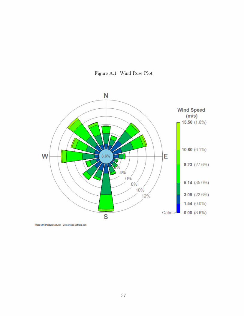
Figure A.1: Wind Rose Plot

37

Table A.5: Effect of Number of Deliveries on PM2.5 Concentration: Interacted withWind Speed



Constant 0.115*** 0.119*** 0.113*** 0.125***(0.0247) (0.0154) (0.0122) (0.00932)

5% Quantile of Wind Speed -0.00704*** -0.00832*** -0.00813*** -0.00880***(0.00169) (0.00108) (0.000896) (0.000684)



Constant 0.0498*** 0.0489*** 0.0433*** 0.0454***(0.0118) (0.00683) (0.00545) (0.00430)

5% Quantile of Wind Speed -0.00242*** -0.00273*** -0.00249*** -0.00269***(0.000696) (0.000438) (0.000374) (0.000292)








*** p<0.01, ** p<0.05, * p<0.1

38

Table A.6: Effect of Coal Stockpiles on PM2.5 Concentration: Interacted with WindSpeed



Constant -1.38e-07 -1.77e-07 -5.54e-07*** -5.31e-07***(4.64e-07) (2.75e-07) (1.62e-07) (1.17e-07)

5% Quantile of Wind Speed 7.28e-08*** 3.33e-08** 5.07e-08*** 4.66e-08***(2.73e-08) (1.69e-08) (1.11e-08) (8.43e-09)



Constant -0.0125* -0.00379 -0.0104*** -0.0125***(0.00736) (0.00538) (0.00374) (0.00264)

5% Quantile of Wind Speed 0.00115*** 0.000459 0.000847*** 0.000950***(0.000429) (0.000326) (0.000240) (0.000176)








*** p<0.01, ** p<0.05, * p<0.1

39

A.2 Additional Results: Quantification of Local Environmental

Damages

Table A.7: Per-ton Social Cost Estimates from the Models that do not control forDirection


numdelivp,t 43.21 13.21 8.04 10.68

Table A.8: Per-KWh Social Cost Estimates from the Models that do not control forDirection


numdelivp,t 0.0231 0.0059 0.0038 0.0053

40

A.3 Additional Figures/Tables: Mortality Rate Regressions

Table A.9: Mortality Rate Summary Statistics: 25 Mile/Over-30

Variable Obs Mean Std. Dev.Mortality Rate: Cardio (Per 1000 People) 47853 0.411 0.104

Mortality Rate: Respiratory (Per 1000 People) 41273 0.105 0.030Mortality Rate: Nervous (Per 1000 People) 32703 0.054 0.018

Mortality Rate: Total (Per 1000 People) 48888 1.162 0.219Mortality Rate: External (Per 1000 People) 33902 0.062 0.020

Population 48888 1328125 1137439PM2.5 (in ug/m3) 48888 12.631 3.912














41







Table A.13: PM2.5 on Mortality Rate: OLS/25 mile/Ages 30+

VARIABLES Cardio MR Resp. MR Nervous MR Total MR External MR

log(PM2.5 + 1) 0.00846** 0.0156*** -0.0177** 0.00267 -0.0235***(0.00355) (0.00551) (0.00882) (0.00273) (0.00703)

Observations 42,988 36,961 29,122 44,021 30,255R2 0.911 0.717 0.790 0.919 0.753





*** p<0.01, ** p<0.05, * p<0.1



log(PM2.5 + 1) 0.0073*** 0.0142*** -0.0229*** -0.0011 -0.0163***(0.0025) (0.0045) (0.0062) (0.0020) (0.0050)

Observations 138,259 112,267 86,815 144,162 89,064R2 0.903 0.737 0.780 0.918 0.729





*** p<0.01, ** p<0.05, * p<0.1

42



log(PM2.5 + 1) 0.0121*** 0.0344*** -0.0187*** 0.0042*** -0.0112***(0.0022) (0.0033) (0.0049) (0.0015) (0.0041)

Observations 1,123,404 839,531 612,645 1,196,452 619,998R2 0.898 0.767 0.830 0.921 0.736





*** p<0.01, ** p<0.05, * p<0.1

Table A.16: PM2.5 on Mortality Rate: IV/25 mile/Ages 30+


log(PM2.5 + 1) 0.134*** 0.469*** 0.239** 0.109*** -0.104(0.0386) (0.0942) (0.0969) (0.0296) (0.0856)

Observations 42,093 36,203 28,558 42,965 29,741R2 0.903 0.609 0.769 0.908 0.752





*** p<0.01, ** p<0.05, * p<0.1

43



log(PM2.5 + 1) 0.237*** 0.443*** 0.292*** 0.200*** -0.128(0.0420) (0.0874) (0.0745) (0.0357) (0.0776)

Observations 134,023 109,051 84,565 139,454 86,894R2 0.871 0.642 0.743 0.877 0.727





*** p<0.01, ** p<0.05, * p<0.1



log(PM2.5 + 1) 0.168*** 0.272*** 0.126*** 0.141*** -0.0236(0.0183) (0.0373) (0.0324) (0.0155) (0.0376)

Observations 1,074,948 803,198 586,163 1,144,422 593,549R2 0.885 0.745 0.823 0.906 0.739





*** p<0.01, ** p<0.05, * p<0.1

44

Table A.19: PM2.5 on Mortality Rate: OLS/25 mile/All Ages


log(PM2.5 + 1) 0.0088** 0.0138** -0.0163* 0.0023 -0.0257***(0.0036) (0.0055) (0.0086) (0.0028) (0.0065)

Observations 42,996 37,054 29,489 44,027 33,708R2 0.916 0.735 0.800 0.926 0.773





*** p<0.01, ** p<0.05, * p<0.1



log(PM2.5 + 1) 0.0073*** 0.0136*** -0.0201*** -0.0012 -0.0213***(0.0025) (0.0045) (0.0060) (0.0020) (0.0046)

Observations 138,259 112,267 86,815 144,162 89,064R2 0.903 0.737 0.780 0.918 0.729





*** p<0.01, ** p<0.05, * p<0.1

45



log(PM2.5 + 1) 0.0100*** 0.0219*** -0.0181*** 0.0003 -0.0208***(0.0024) (0.0036) (0.0057) (0.0019) (0.0043)

Observations 381,425 296,463 224,652 403,410 258,221R2 0.911 0.779 0.834 0.932 0.760





*** p<0.01, ** p<0.05, * p<0.1



log(PM2.5 + 1) 0.0117*** 0.0340*** -0.0180*** 0.0040*** -0.0139***(0.0021) (0.0033) (0.0048) (0.0015) (0.0038)

Observations 1,123,923 842,528 620,522 1,197,302 716,960R2 0.910 0.788 0.839 0.933 0.760





*** p<0.01, ** p<0.05, * p<0.1

46

Table A.23: PM2.5 on Mortality Rate: IV/25 mile/All Ages


log(PM2.5 + 1) 0.134*** 0.461*** 0.196** 0.117*** -0.0739(0.0377) (0.0887) (0.0850) (0.0286) (0.0648)

Observations 42,101 36,293 28,921 42,965 33,079R2 0.908 0.636 0.787 0.914 0.773





*** p<0.01, ** p<0.05, * p<0.1



log(PM2.5 + 1) 0.235*** 0.417*** 0.256*** 0.197*** -0.120**(0.0409) (0.0826) (0.0672) (0.0346) (0.0518)

Observations 134,068 109,352 85,597 139,520 97,630R2 0.881 0.679 0.766 0.890 0.752





*** p<0.01, ** p<0.05, * p<0.1

47



log(PM2.5 + 1) 0.193*** 0.159** 0.218*** 0.170*** -0.0951**(0.0378) (0.0788) (0.0607) (0.0308) (0.0452)

Observations 366,480 284,522 215,326 387,165 247,878R2 0.893 0.771 0.816 0.908 0.758





*** p<0.01, ** p<0.05, * p<0.1



log(PM2.5 + 1) 0.165*** 0.260*** 0.109*** 0.134*** -0.0467(0.0182) (0.0367) (0.0332) (0.0149) (0.0293)

Observations 1,075,444 806,053 593,727 1,145,183 686,196R2 0.900 0.770 0.834 0.921 0.760





*** p<0.01, ** p<0.05, * p<0.1

48

Table A.27: PM2.5 on Mortality Rate: OLS/25 mile/30+/Only CSp,t


log(PM2.5 + 1) 0.0086** 0.0156*** -0.0179** 0.0027 -0.0234***(0.0036) (0.0055) (0.0088) (0.0027) (0.0070)

Observations 42,988 36,961 29,122 44,021 30,255R2 0.911 0.717 0.790 0.919 0.753





*** p<0.01, ** p<0.05, * p<0.1



log(PM2.5 + 1) 0.0073*** 0.0142*** -0.0229*** -0.0011 -0.0163***(0.0025) (0.0045) (0.0062) (0.0020) (0.0050)

Observations 138,259 112,267 86,815 144,162 89,064R2 0.903 0.737 0.780 0.918 0.729





*** p<0.01, ** p<0.05, * p<0.1

49



log(PM2.5 + 1) 0.0101*** 0.0226*** -0.0202*** 0.0005 -0.0170***(0.0024) (0.0037) (0.0059) (0.0019) (0.0047)

Observations 381,277 295,534 221,833 403,183 226,132R2 0.901 0.758 0.823 0.922 0.734





*** p<0.01, ** p<0.05, * p<0.1



log(PM2.5 + 1) 0.0121*** 0.0344*** -0.0187*** 0.0042*** -0.0112***(0.0022) (0.0033) (0.0049) (0.0015) (0.0041)

Observations 1,123,404 839,531 612,645 1,196,452 619,998R2 0.898 0.767 0.830 0.921 0.736





*** p<0.01, ** p<0.05, * p<0.1

50

Table A.31: PM2.5 on Mortality Rate: IV/25 mile/30+/Only CSp,t


log(PM2.5 + 1) 0.230*** 0.473*** 0.0721 0.182*** 0.00875(0.0465) (0.0984) (0.0875) (0.0359) (0.0811)

Observations 42,093 36,203 28,558 42,965 29,741R2 0.885 0.607 0.788 0.886 0.754





*** p<0.01, ** p<0.05, * p<0.1



log(PM2.5 + 1) 0.251*** 0.424*** 0.282*** 0.210*** -0.114(0.0454) (0.0852) (0.0732) (0.0380) (0.0758)

Observations 134,023 109,051 84,565 139,454 86,894R2 0.867 0.650 0.745 0.873 0.728





*** p<0.01, ** p<0.05, * p<0.1

51



log(PM2.5 + 1) 0.216*** 0.228*** 0.277*** 0.190*** -0.0757(0.0404) (0.0832) (0.0716) (0.0335) (0.0741)

Observations 366,338 283,632 212,573 386,973 217,146R2 0.876 0.739 0.795 0.888 0.735





*** p<0.01, ** p<0.05, * p<0.1



log(PM2.5 + 1) 0.170*** 0.275*** 0.112*** 0.142*** -0.0200(0.0187) (0.0377) (0.0324) (0.0158) (0.0392)

Observations 1,074,948 803,198 586,163 1,144,422 593,549R2 0.885 0.744 0.824 0.906 0.739





*** p<0.01, ** p<0.05, * p<0.1

52

B Data Appendix

B.1 Data Sources: Coal Procurement

For coal inventories and consumption, we use Forms EIA-906 (for 2002-2007) and EIA-

923 (for 2008-2012). Data on coal stocks for 2002-2012 are considered proprietary; we

obtained a research contract with the Energy Information Administration (EIA) in order

to use these data for our analysis.

For coal purchases and prices, we use Forms EIA-423 (2002-2007) and EIA-923 (2008-

2012). These data are at the “order level”; an “order” as defined by these forms is based

on the following criteria:

“Data on coal received under each purchase order or contract with a supplier should be

reported separately. Aggregation of coal receipt data into a single line item is allowed if

the coal is received under the same purchase order or contract and the purchase type,

fuel, mine type, State of origin, county of origin, and supplier are identical for each

delivery.”

In some specifications, we consider the “number of deliveries” to a plant in each month,

as measured by the number of orders each plant reports on the form for each month-of-

sample. This measure for the number of deliveries may be under-estimated to the extent

that deliveries under the same purchase order are aggregated as described in the above

quotation.

The variables included in this purchase dataset include month of purchase, quantity

purchased, delivered price, heat content, sulfur content, ash content, origin of coal, and

whether the delivery came from a long-term contract or the spot market.

53

the local environmental consequences of coal …economics.ucdavis.edu/events/papers/112jha.pdfthe...

Documents