the locomotive assignment problem with distributed power … · 2019-11-28 · the locomotive...

CIRRELT-2019-55

The Locomotive Assignment Problem with Distributed Power at the Canadian National Railway Company Camilo Ortiz-Astorquiza Jean-François Cordeau Emma Frejinger

November 2019

The Locomotive Assignment Problem with Distributed Power at the Canadian National Railway Company

Camilo Ortiz-Astorquiza1,2, *, Jean-François Cordeau1,3, Emma Frejinger1,4

1 Interuniversity Research Centre on Enterprise Networks, Logistics and Transportation (CIRRELT) 2 Departamento de Matemáticas, Pontificia Universidad Javeriana, Bogotá, Colombia 3 Department of Logistics and Operations Management, HEC Montréal, 3000 Côte-Sainte-

Catherine, Montréal, Canada H3T 2A7 4 Department of Computer Science and Operations Research, Université de Montréal, P.O. Box

6128, Station Centre-Ville, Montréal, Canada H3C 3J7

Abstract. Some of the most important optimization problems faced by railway operators arise from the management of their locomotive fleet. In this paper, we study a general version of the locomotive assignment problem encountered at the tactical level by one of the largest railroads in North America: the Canadian National Railway Company (CN). We present a modeling framework with two integer linear programming formulations and contribute to the state of the art by allowing to decide each train's operating mode (distributed power or not) over the whole (weekly) planning horizon without partitioning it into smaller time windows. Given the difficulty to solve the problem, one of the formulations is enhanced through various refinements such as constraint relaxations, preprocessing and fixed cost approximations. We thus achieve a significant reduction in the required computational time to solve instances of realistic size. We also present two versions of a Benders decomposition-based algorithm to obtain feasible solutions. On average, it allows to reduce the associated computational time by two hours. Results from an extensive computational study and a case study with data provided by CN confirm the potential benefits of the model and solution approach. Keywords. Locomotive planning, network optimization, railway transportation, integer programming. Acknowledgments: The authors gratefully acknowledge the close collaboration with personnel from the Canadian National Railway Company (CN) and the funding received through the CN Chair in Optimization of Railway Operations. This research is also funded by the Natural Sciences and Engineering Research Council of Canada (NSERC) Collaborative Research Grant. Computations were made on the supercomputer beluga, managed by Calcul Québec and Compute Canada. The operation of this supercomputer is funded by the Canada Foundation for Innovation (CFI), the Ministère de l'économie, de la science et de l'innovation du Québec (MESI) and the Fonds de recherche du Québec - Nature et technologies (FRQ-NT).

Results and views expressed in this publication are the sole responsibility of the authors and do not necessarily reflect those of CIRRELT.

Les résultats et opinions contenus dans cette publication ne reflètent pas nécessairement la position du CIRRELT et n'engagent pas sa responsabilité. _____________________________ * Corresponding author: [email protected]

Dépôt légal – Bibliothèque et Archives nationales du Québec Bibliothèque et Archives Canada, 2019

© Ortiz Astorquiza, Cordeau, Frejinger and CIRRELT, 2019

1 Introduction

Locomotive planning plays a crucial role in the overall performance of railway compa-nies. The high cost of locomotives and the large number of them required to satisfytrain schedules make of the locomotive fleet one of their most valuable assets, generallyrepresenting an investment in the order of billions of dollars. Therefore, optimizationtools that help in the locomotive planning process are potentially highly valuable. Al-though previous studies have shown significant potential savings, many railway com-panies still rely on human experience to solve the complex decision-making problemsrelated to locomotive planning. Moreover, proper management can have significantsocial and environmental impacts. For example, the railway industry represents one ofthe most important means of transportation in North America. In Canada only, over900,000 tons of freight were transported on a daily basis in 2017 [19]. In this paperwe focus on a tactical locomotive planning problem faced by one of the largest railwaycompanies in North America, the Canadian National Railway Company (CN).

The Operations Research (OR) literature on locomotive fleet management distin-guishes two main problem types that match the decision process of most railways,namely, a tactical and an operational optimization problem. The need to resort to asequential planning approach is a consequence of both the complexity of the problemsand the types of decisions to be made. At the tactical stage, it has been referred toas the Locomotive Assignment Problem (LAP) [21] whereas at the operational level itis usually known as the Locomotive Routing Problem (LRP) [22]. In brief, the LAPconsists of determining the number and types of locomotives assigned to each train of agiven schedule so that power requirements and flow balance of locomotives at stationsare met while minimizing an objective function. The typical train schedule is a weeklyplan to be repeated over a three or four-month period. The goal in the LAP is toobtain a guideline on how to assign locomotive types to trains and reposition them inthe network so that the plan is repeated every week. Then, the LRP is solved weeklyto determine the actual sequence of trains to be operated by each specific locomotivewhile honoring other constraints and minimizing the cost.

In railway transportation, especially for freight in North America, typically thereis more than one locomotive assigned to operate each train either because the demandfor horse power (HP) cannot be satisfied otherwise or because operating main-line(ML) trains that are usually long and heavy on long distances or specific corridorswith difficult geographic conditions require reliable consists. A consist is defined as agroup of locomotives traveling together. More importantly, in recent years, CN andmany other railway operators have started moving from the conventional mode whereall the active locomotives travel together at the head of the train to distributed power(DP), where locomotives can be interspersed throughout the length of the train. DPis a relatively recent technology [10] which has yielded several patents in the last twodecades. However, it also brings an extra level of complexity to the planning problem.On the one hand, DP reduces the in-train forces permitting an increase in the lengthand weight of the train. It also reduces fuel consumption, wear on various componentsand the possibility of derailment. On the other hand, setting up and separating thelocomotives that travel on DP mode is more time consuming and not all locomotivespossess the right equipment to be used in this mode. Thus, in this article, we study ageneral version of a tactical LAP denoted LAP-DP. We continue this section with anoverview of related work followed by a statement of our contributions.


CIRRELT-2019-55 1

1.1 Literature Review

Several articles in the broader context of locomotive scheduling have been publisheddating back to the mid 1970’s. Here we mention those that we consider the mostrelevant ones for this paper mainly based on the level of planning but we refer thereader to the survey papers [9] and [17] for a more complete review of the literature.We note that the problem names and their definitions may vary in related articles, notnecessarily following the classification discussed here.

One of the first works addressing the LAP with a locomotive fleet composed ofdifferent locomotive types was that of Florian et al. [12]. In this case, consists canbe formed of one or more locomotive types to meet HP requirements. The authorsproposed a multicommodity network flow-based model and a Benders decompositionalgorithm to solve the problem. Their model was later generalized by Ziarati et al.[23] to include other operational constraints in what they denoted as an LAP at theoperational strategic level requiring no repetitiveness of the solution. [23] proposed asolution method for full size instances on CN data from 1995 (approx. 2,000 trains perweek and 1,200 locomotives) based on dividing the time horizon into a set of rollingand overlapping 1-day time windows. Every time slice is optimized using a branch-and-bound procedure in which the Linear Programing (LP) relaxations are solved witha Dantzig-Wolfe decomposition. The authors also considered maintenance constraintsfalling into the category of what we denote as the LRP. In a subsequent paper, [24]presented an improved solution methodology denoted branch-first, cut-second whichsignificantly reduces the LP relaxation gap and the overall computing time.

Cordeau et al. [7, 8] presented exact algorithms based on Benders decomposition tohandle the simultaneous assignment of locomotives and cars of passenger transporta-tion for Via Rail Canada. Ahuja et al. [2] and Vaidyanathan et al. [21] proposedILP formulations for a tactical version of the LAP considering several realistic char-acteristics in collaboration with CSX Transportation. Their formulations are basedon a space-time network representation and can be described under the umbrella ofmulticommodity network design problems with integer flows. [2] proved that the LAPis an NP-hard problem which in turn implies that the LAP-DP also belongs to thisclass of problems. The authors also present heuristic methods to solve the modelsmainly by removing fixed-charge variables and solving the 1-day version repeatedlyover the full week. Their full size instances contain approximately 3,300 trains and3,300 locomotives among five locomotive types.

Vaidyanathan et al. [21] included additional operational constraints and proposedan improved ILP formulation based on assigning only predefined consists. This ideafollowed from the important observation that since an integral number of locomotivesmust be assigned, it is very unlikely that there is a consist satisfying exactly the trainHP [24]. In reality, the function of HP over the set of consists is not continuous buta stepwise function. More importantly, these steps are typically of a few hundreds ofHP which in turn implies a significant gap between the LP relaxation and the ILPsolution. Moreover, several side constraints can be implicitly handled in the predefinedconsists. Vaidyanathan et al. [21] discuss the benefits of having a pure consist-basedformulation for the LAP where both active and non-active locomotives travel in thenetwork as consists. Later, Piu et al. [16] proposed an optimization model to definethe initial set of consists and Jaumard and Tian [13] proposed a column generationapproach for a similar variant of the LAP.


2 CIRRELT-2019-55

More recently, Powel et al. [18] and Bouzaiene-Ayari et al. [6] presented anapproach based on Approximate Dynamic Programming (ADP) to solve locomotivescheduling problems for Norfolk Southern. The authors proposed three optimizationmodels distinguished mainly by the level of detail that define the set of locomotiveswhich is tightly related with the level of planning. They refer to this family of models asPLASMA (Princeton Locomotive and Shop MAnagement system). First, they considera strategic variant denoted as single commodity formulation (PLASMA/SC) where alllocomotives are assumed to be of the same type. Then, they consider a multicommodityformulation with four locomotive types (PLASMA/MC) and finally a multi-attributeversion in which each locomotive is identified individually (PLASMA/MA). Note thatthe PLAMA/MC and PLASMA/MA versions are similar to what we denote the LAPand LRP, respectively. One of the important contributions of Bouzaiene-Ayari et al.[6] was to include and efficiently handle several sources of uncertainty, especially thoserelating to time delays. However, as the authors point out, ADP seems to be well suitedto handle high levels of detail, including uncertainty, but is less skilled at managing aglobal vision of flows around the network over time. This means that ADP is possiblynot the best approach to deal with repeatable solutions, i.e., matching ending withbeginning inventories, which is our focus.

1.2 Contributions

To the best of our knowledge, deciding of the operating mode (DP or conventional) hasnot been included in the optimization models proposed in the literature nor any benefit(e.g., reduction in the HP required) that depends on the type of consist. Also, we notethat there is no solution methodology of a general and realistic version of an LAPin which one considers repetitiveness in the solution without partitioning the trainschedule into smaller time windows. This cyclic behavior is an important modelingaspect when following a sequential planning approach to facilitate the implementationof the subsequent problem solution. Furthermore, depending on the train schedule,trains may operate only a few days per week which can yield suboptimal solutionswhen solving a daily problem. Thus, the main contributions of this article are thefollowing.

– We introduce a general version of an LAP denoted as LAP-DP in which the modeof operation of the trains is part of the decision process. Under this umbrellawe consider the benefits in the HP required depending on consist configurationand we show how it greatly impacts the objective function value. Additionally,we incorporate other real-life considerations in the model such as repositioningof inactive locomotives at intermediate stations and consist busting which areexplained in detail in the following sections.

– We present two Integer Linear Programming (ILP) formulations to model theLAP-DP and we develop various enhancements on one of them to improve thecomputational performance when solved with a general-purpose solver. Amongother ideas, we propose constraint relaxations, approximation of fixed costs andcriteria to select predefined consists available to be assigned. With the enhancedformulation we obtain good solutions, compared to actual operations, for real-sizeinstances of the problem within a time limit of 6 hours. Without these refinements


CIRRELT-2019-55 3

and proper implementation of the modeling framework it is not possible to evenobtain feasible solutions within this computing time limit.

– We also develop two versions of an algorithm based on Benders decomposition [4]to obtain feasible solutions in reasonable time and test different variants of thesealgorithms to assess their performance. On average, there is a time improvementof almost two hours to find the first feasible solution in comparison with theenhanced formulation for the full-size instances. Moreover, the results indicatethat the Benders-based algorithms are less dependent on the number of threadsused in the experiments.

– We present results and insights from a case study based on real data and guidanceprovided by CN for ML freight trains as well as local and yard services requiringplanned locomotive power. All the solutions obtained with the model indicatesignificant potential savings in comparison with the actual operations.

– We perform an extensive computational study to assess the performance of theformulations on realistic instances. Through a sensitivity analysis on variousparameters of the models, we assess the characteristics of the solutions as well asthe performance of the algorithms. The results show that there is an importantimpact on both solutions and algorithmic performance when emphasizing certainparameters of the objective function and some constraints.

1.3 Paper Structure

The remainder of the paper is organized as follows. In Section 2 we describe theLAP-DP in detail and in Section 3 we present the modeling framework along with twoILP formulations. In Section 4 we describe the algorithmic refinements on one of theformulations and two algorithms based on Benders decomposition for the LAP-DP. InSection 5 we present the computational experiments and the case study and conclusionsfollow in Section 6.

2 Problem Description

At the tactical level, the goal is to obtain a cyclic solution that provides a guidelinefor the subsequent levels of planning. Thus, it becomes unnecessary and rather coun-terproductive to determine the routes of individual locomotives at this stage becausetheir operational conditions and initial positions in the network will vary from week toweek. In addition, the train schedule may suffer small changes every week and, moreimportantly, there are decisions associated with individual locomotives that would bedifficult or impossible to comply with when planning three months in advance. Instead,the problem is modeled by aggregating locomotives into significant types, i.e., assumingthat locomotives with similar specifications and costs are actually indistinguishable. Inthis context, it is important to emphasize that the LAP can only be implemented inpractice jointly with an LRP solution.

In particular, the LAP-DP consists of determining the optimal assignment of lo-comotive types to trains and the choice of operating mode while satisfying power re-quirements and flow balance for a given 7-day train schedule. The force required topull a train is often expressed in terms of HP which can be met by selecting a set of


4 CIRRELT-2019-55

locomotives, possibly of different types. Hence, the main output of the LAP-DP is anassignment of consists to trains.

2.1 Problem Data

The input of the LAP-DP mainly consists of a weekly train schedule with the corre-sponding HP demand values and a set of available locomotives partitioned into types.Let K be a set of locomotive types and AT the set of train legs indexed by l ∈ AT .

Trains legs: Each train leg l ∈ AT is defined by a type, origin and destination sta-tions, a length, a tonnage tl, times of departure and arrival, and a parameterβl called Horse Power to Tonnage (HPT). The train type determines whether atrain operates in the mainline network, which typically implies heavy, long dis-tance trains, or if it is a local or yard service. The HPT is based on geographicaland operational conditions and it allows to approximate how much HP is neededto pull the tonnage of the train.

Locomotives: Associated with each locomotive type k ∈ K are the number of avail-able locomotives fk, the HP hk, the weight of a locomotive wk, a binary parameterdpk indicating whether it is DP equipped, the number of axles λk and an indicatorthat determines whether it generates DC or AC power. Let B and D be the setsof locomotive types that generate AC and DC power, respectively.

Network: Information on the rail network is assumed to be available such as eachtrain route Rl, the railroad distance r(i, j) between stations i and j and powerchange stations, which are predefined points in the network where some trainsmay stop for a consist change.

Costs: We consider fuel consumption costs which depend on the locomotive type, thetrain and the diesel cost. Also, we consider a track maintenance cost associatedwith the usage of the railroad. There is an ownership cost gk that correspondsto the weekly cost of using a locomotive of type k. Finally, there are crew coststhat depend on the duration of the train as well as the train type.

2.2 Power Requirements

One of the main constraints of any LAP is to assign sufficient locomotives of theright types so that one ensures the HP required to pull each train. The typical HPapproximation for a given train leg l is done using βltl. However, an important aspectthat may yield significant savings and is not being considered using this approximationis that the HPT changes when a train is operated under DP or when the assignedconsist is formed of AC locomotives only. Therefore, a more precise approximation ofthe HP required is

HPl =

βltl if conventional mode

βAl tl if conventional mode and all AC locomotives

(βl − θl)tl if DP mode

(βAl − θl)tl if DP mode and all AC locomotives,

(1)


CIRRELT-2019-55 5

where βAl and θl model the values of HPT if only AC locomotives are assigned and thediscount on HPT for using DP, respectively.

Another aspect to consider is the power change stations where trains may modifyconsists. These are well-defined stations in the schedule since it is known where theHPT varies considerably from one part of the route to the next. One way to includethis feature is by splitting the original train by modifying the origin-destination (OD)into the corresponding parts at power change stations as if they were separate trainsin a preprocessing stage.

2.3 Consist Busting and Train-to-Train Connections

Consist busting is an important decision in locomotive scheduling which plays a majorrole in the objective function of existing models, especially for those at the operationallevel. We say that a consist is busted if, after arriving at its destination station, thelocomotives are separated and become available individually. Otherwise, when thearriving consist is assigned without changes to a departing train, we refer to it as atrain-to-train connection. In Section 5.2 we describe in detail how we handle train-to-train connections.

2.4 Flow Balance and Power Availability

An important aspect in locomotive planning is ensuring that there are sufficient loco-motives of each desired type at each station to satisfy the train schedule. However,the network is usually unbalanced because some stations require more HP than theyreceive through the arriving trains or vice-versa. Stations are called sources when thetotal HP of departing trains exceeds that of arriving trains and sinks in the oppositesituation. Therefore, locomotives must be repositioned by other means than as activepower on scheduled trains. This can be done in two ways: (i) deadheading (DH), whichindicates that locomotives travel using the scheduled trains but are not pulling, and (ii)light traveling, which consists of sending groups of locomotives where only the leadingone is active and they do not have additional railcars attached. Note that DH is lesscostly but in many cases the only or most rapid way of repositioning locomotives isthrough light traveling.

An additional feature included in the LAP-DP, that to the best of our knowledgehas not been addressed before, is to allow extra DH. What we denote as “extra” DHis common in practice and is formed of two parts. First, when there is an active train-to-train connection the non-active locomotives are allowed to stop or be added at theconnecting station. Second, DH of locomotives that occurs between pairs of stationsother than the origin and destination pair of each scheduled train, i.e., intermediatestations in the train route. Allowing DH locomotives to be dropped off and picked upin the middle of the train route at predefined stations has a significant impact in thesolution and computing time.

2.5 Additional Constraints

Several side constraints and preferences are considered in the LAP-DP to better capturethe requirements that arise in practice. For example, limiting the number of (active)locomotives and the number of active axles per train (al) as well as avoiding mixes of AC


6 CIRRELT-2019-55

with DC locomotives. Some of these requirements are desirable but not mandatory. Wecan also impose that certain trains operate under DP or conventional mode dependingon the length and weight of the train and we promote certain characteristics in thesolution by means of weights in the objective function. Other common features inlocomotive planning such as the use of foreign power (leasing locomotives from otherrailways), train delays and maintenance constraints are treated at the operational level.

3 Modeling Framework

We model the LAP-DP via a space-time network that represents the physical railroadand the train schedule simultaneously. Time units are in minutes and each locomotivetype is considered a commodity to be routed on the network. LetG = (N,A) be a graphwith N the set of nodes and A the set of arcs. Each node i ∈ N is associated with threeattributes, namely, station number, time and type, whereas each arc a ∈ A representsan activity such as a train leg, a waiting period, or repositioning of locomotives, amongothers. As in a network flow problem [3], the flow of a particular commodity on an arcrepresents the assignment of this locomotive type to the corresponding activity. Wenote that most of the notation used throughout this article is inherited from airlineplanning problems and from previous work on the LAP.Note that we refer indistinctlyto a train arc and a train leg. Tables 1 and 2 summarize the main notation forparameters and sets used throughout the paper.

Table 1: Summary of main parameters

hk, λk, wk Horsepower, number of axles and weight of locomotives of type k

dpk Binary parameter indicating if locomotives of type k are DP equipped

fk Number of available locomotives of type k

tl Tonnage of train l ∈ AT

βl, βAl Standard and AC-only HPT for train l ∈ AT

mA,mT ,mD,mDH Maximum number of locomotives (active, total, DP, DH) per train

r(i, j) Railroad distance between stations i and j

gk Weekly ownership cost for a locomotive of type k

ckl Per unit cost of assigning an active locomotive of type k to train l

dkl Per unit cost of assigning a non-active locomotive of type k on arc l

θl Discount on the train HPT for operating on DP

al Maximum number of active axles for train l ∈ AT

ρck Number of locomotives of type k in consist c

3.1 Space-time Network

Figure 1 depicts an example of a space-time network with four trains represented withthe bold arcs and four different stations. The dashed and bold-dotted arcs correspondto the cyclic behavior of the solution, light travel and extra DH arcs, respectively. Wealso show examples of train-to-train arcs in the figure but we omit the representationof all extra DH arcs to simplify the diagram.The set of nodes is partitioned into arrival (NA), departure (ND) and ground nodes


CIRRELT-2019-55 7

Table 2: Summary of sets

K Set of locomotive types or commodities

N , A Sets of nodes and arcs in the space-time network

NA, ND Sets of arrival and departure nodes

NG = NI ∪NR ∪NE ∪NDP Set of ground nodes (initial, grd-arr, grd-dept and DP)

AT Set of train arcs

AG, ADP and AL Sets of inter-ground, DP and light-travel arcs

AC = AR ∪ AE ∪ AQ Sets of arrival-ground, ground-departure, and train-to-train arcs

ADH Set of extra deadheading arcs

I[i], O[i] Sets of inbound and outbound arcs for each i ∈ NS Set of arcs that cross the checkpoint

B, D Sets of locomotive types that have AC (or DC) power

Rl Set of stations in the route followed by train l

E(l, i, j) ⊆ ADH Extra DH arcs available between stations i and j in Rl

Cl Set of predefined feasible consists for train l

CDP Set of predefined consists using DP mode

DP node

grd-dept node grd-arrival node

departure node arrival node

initial node

Station 1

Station 2

Station 3

Station 4

Train 1

Train 2

Train 3 Train 4

tr-to-tr

tr-to-tr

Extra DH arc

Figure 1: Example of space-time network on four trains and four stations


8 CIRRELT-2019-55

(NG). A train arc goes from a departure to an arrival node and the correspondingtrain information defines the station numbers and times for these nodes. Groundnodes are used to represent the events of locomotives when they are not assigned toa train, i.e., they are at a station. The set of ground nodes is further partitioned intoground-arrival NR, ground-departure NE , ground-initial NI and DP NDP nodes. Foreach arrival node there is an arrival-ground node and for each departure node thereis a ground-departure node. Each one of them has the same station number as itscorresponding arrival or departure node. Each arrival-ground node has the time asits associated arrival node plus an input parameter that models the time for consistbusting. For ground-departure nodes a value is subtracted from the departure timeto model the time of creating a consist. A similar procedure is followed to create DPnodes. However, we should note that not every train will be allowed to operate on DPmode. Finally, we have one initial ground node at time zero for each station.

In the set of arcs we consider train arcs AT , DP arcs ADP , arrival-ground AR,ground-departure (AE) and train-to-train (AQ) connection arcs (AC = AR∪AE ∪AQ).Moreover, for each station we sort by time the ground nodes and create an inter-ground arc between each sequential ground node forming the set AG of inter-groundarcs. After sorting the nodes, the last ground node of each station is connected withthe corresponding initial ground node to model the cyclic behavior of the LAP-DP.

The set of extra DH arcs ADH consists of two types of arcs: first, those that are nottrain arcs and outbound a departure node and arrive in an appropriate ground nodeof an intermediate station of the train route satisfying the travel time. Second, thosethat depart from an appropriate ground node of an intermediate station and finishat the arrival node. Note that using this construction we do not permit all possiblecases of partial DH, only those that depart from or arrive to the associated origin ordestination station of the train. We also limit the number of extra DH arcs by creatingonly those to or from intermediate stations with few in or out scheduled trains sincethey are more likely to need extra DH.

Finally, when an arc crosses the checkpoint, e.g., the arrival time is greater thanthe time horizon limit, we modify its destination and define the time attribute of thenode such that it becomes the extra minutes after the checkpoint that is initially past.The set S is formed by all the arcs crossing the checkpoint as well as the cycle arcs.

3.2 Generating Light Traveling Arcs

Light travel arcs play a major role in the network representation when solving theLAP-DP. Including all possibilities of light travel arcs is not desired because the sizeof the network would increase considerably. The goal is then to select a suitable subsetof light travel arcs for which we follow a similar approach as that of [2]. In particular,we determine origin and destination stations of light travel arcs and their frequency byestablishing the flow of HP in the network without considering the time component.We thus solve a minimum cost flow problem [3] where the supply or demand of eachnode is given by an approximation of the total inbound HP minus the total outboundHP. Nodes with positive supply values represent power sinks and stations with negativesupply values are power sources. We define the objective value coefficient for arc (i, j)


CIRRELT-2019-55 9

as

eij =

r(i, j) if nOpij ≤ 2

r(i, j)α if nOpij ∈ (2, α)

r(i, j)α2 otherwise,

where α is an input parameter and nOpij is the number of scheduled trains to operatefrom station i to station j. With this definition we discourage the flow on arcs in thespace network when there are more than a given number of trains that operate an ODpair assuming that those locomotives can be deadheaded. This partly accounts for notsaturating OD pairs using light travel arcs. Note that if long distance light travel isnot desirable, as in our case study, arcs with a distance above a threshold value can beremoved.

Finally, we create light travel arcs between a pair of stations if the correspondingsolution flow is above a given minimum threshold value. We also have an input param-eter to establish how many light travel arcs are created for such pairs. To avoid thecreation of extra nodes in the space-time network, we generate light travel arcs con-veniently using the current set of ground nodes. In particular, we use ground-arrivalnodes as origins without affecting the representation of the model because it is thenwhen locomotives become available to be sent elsewhere. In practice, it is possible thatthe locomotives are not sent exactly at that time as long as it is ensured that theyarrive to their destination at the required time. Similarly, for destination nodes wechoose the first ground node that is available after the corresponding travel time. Atthat time it is when the locomotives are possibly needed and can be made available.

3.3 A Consist-and-Locomotive Flow-Based Formulation

A common way of modeling an LAP is through integer flows traveling in the space-timenetwork that represent the number of locomotives of each type on each arc. Previousworks [e.g., 2] have shown that the performance of this type of formulation is very poorin terms of computing time. We present a new Locomotive-Based Formulation (LBF)for the particular case of the LAP-DP in the Online Appendix. However, preliminarycomputational experiments confirmed the slow performance of this type of formulationwhen solved with a general-purpose solver.

Another approach to model the problem is to consider a predefined set of feasibleconsists C and to decide through binary variables whether a consist is assigned to atrain or not [21]. In addition, we must also incorporate the operating mode in thedecision. Let Cl ⊆ C be the subset of feasible consists for train leg l, including DP andconventional consists, and ρck be the number of locomotives of type k in consist c ∈ Cl.

Also, consider the subset CDP of consists that operate on DP and its complement CDP ,the set of consists on conventional mode. As mentioned before, there are numerousbenefits to using a formulation based on consists instead of locomotive flows. Forexample, we use the sets Cl to implicitly take into account the HP requirements foreach train and the benefits of using AC-only or DP mode, equivalently to equation(1). Moreover, several side constraints that appear in the LBF can be handled in thedefinition of Cl.

Let xcl be a binary variable taking value 1 if consist c is assigned to arc l ∈ AT ∪AC ∪ ADP and 0 otherwise, and let ykl be the number of non-active locomotives oftype k assigned to arc l ∈ A. Note that since DP consists have to be busted at arrival


10 CIRRELT-2019-55

stations, we still need to define the y variables as locomotive flows instead of consists ofnon-active locomotives. Therefore, we propose a Consist-and-Locomotive Flow-basedformulation (CLF) that is more flexible than a pure consist-based approach in dealingwith the repositioning of locomotives and therefore likely to benefit more from extraDH arcs. Also, let zl = 1 if arc l ∈ AC ∪ AL is used and 0 otherwise. Finally, ul arevariables to control a soft constraint that determines the total number of active axlesper train.

We denote by ckl the operational cost of assigning an active locomotive of type kto train l, which is a function of the track maintenance and fuel consumption costs.The costs dkl vary depending on the arc l, e.g., if l ∈ AT ∪ADH , dkl corresponds to thecost of deadheading a locomotive of type k using arc l whereas if l ∈ AL, dkl representsthe unit cost of light traveling a locomotive of type k on arc l. Fixed costs p and blrepresent the cost of activating an arc in the network, which in this case model thefixed costs of busting and light travel, respectively. In the case of light travel arcs itcorresponds to the associated crew and fuel costs that depend on l. The fixed cost pof busting a consist as well as the penalties and preferences are more subjective anddepend on how much weight the user wants to place on certain characteristics of thesolution. Then, let x be the vector of decision variables, the total cost TotCLF (x) canbe written as

TotCLF(x) =∑k∈K

∑l∈AT

ckl∑c∈Cl

ρckxcl +

∑k∈K

∑l∈AC∪ADP

dkl (ykl +∑c∈Cl

ρckxcl )

+∑k∈K

∑l∈AT∪ADH∪AG∪AL

dkl ykl +

∑k∈K

∑l∈S

gk(ykl +∑c∈Cl

ρckxcl ) +

∑l∈AR

pzl +∑l∈AL

blzl

+∑l∈AT

ul + PCLF (x),

where PCLF (x) is a function associated with weights for penalties and preferences ofsolution features such as mix AC-DC consists and DP, among others. Then, giventhe sets I[i] and O[i] of inbound and outbound arcs of node i ∈ N , respectively, andE(l, i, j) the set of extra DH arcs between stations i and j associated with train routeRl, the CLF can be stated as


CIRRELT-2019-55 11

minimize TotCLF(x) (2)

subject to∑c∈Cl

xcl = 1 ∀ l ∈ AT (3)

∑l∈I[i]

xcl =∑l∈O[i]

xcl ∀ i ∈ NA ∪ND, c ∈ Cl (4a)

∑l∈I[i]

ykl =∑l∈O[i]

ykl ∀ i ∈ NA ∪ND ∪NI , k ∈ K (4b)

∑l∈I[i]

(ykl +∑c∈Cl

ρckxcl ) =

∑l∈O[i]

ykl ∀ i ∈ NR, k ∈ K (4c)

∑l∈I[i]

ykl =∑l∈O[i]

(ykl +∑c∈Cl

ρckxcl ) ∀ i ∈ NE ∪NDP , k ∈ K (4d)

∑k∈K

∑l∗∈E(l,i,j)

ykl∗ +∑k∈K

∑c∈Cl

ρckxcl ≤ mT ∀ l ∈ AT , i, j ∈ Rl (5)


12 CIRRELT-2019-55

∑k∈K

(ykl +∑c∈Cl

ρckxcl ) ≤ mT zl ∀ l ∈ AC (6)

∑k∈K

(ykl +∑c∈Cl

ρckxcl ) ≤ mT

∑c∈Cl∗∩CDP

xcl∗ ∀ l = (i, j) ∈ ADP , l∗ ∈ AT ∩O[j] (7)

∑k∈K

ykl ≤ mT zl ∀ l ∈ AL (8)∑l∈O[i]:l∈AQ

zl ≤ 1 ∀ i ∈ NA (9)

∑l∈I[i]:l∈AQ

zl ≤ 1 ∀ i ∈ ND (10)

∑k∈K

∑c∈Cl

ρckxcl ≥ 2zl ∀ l = (i, j) ∈ AQ, j ∈ ND (11)

zl ≤ 1−∑

c∈Cl∩CDP

xcl∗ ∀ l ∈ AQ ∩O[j], l∗ = (i, j) ∈ AT (12)

∑c∈Cl∩CDP

xcl ≤ 1−∑

l∗∈AQ∩I[j]

zl∗ ∀ l = (i, j) ∈ AE (13)

∑l∈I[i]:l /∈AE

(zl +∑

c∈Cl∩CDP

xcl ) ≤ 1 ∀ i ∈ ND (14)

zl∗ ≤ 1−∑

c∈Cl∩CDP

xcl ∀ l∗ = (i, j) ∈ AE , l ∈ ADP ∩ I[j] (15)

∑c∈Cl

∑k∈K

λkρckxcl − ul ≤ al ∀l ∈ AT (16)

∑l∈S

(ykl +∑c∈Cl

ρckxcl ) ≤ fk ∀ k ∈ K (17)

xcl ∈ Z+ ∀ l ∈ AT ∪AC ∪ADP , c ∈ Cl (18)

ul ∈ Z+ ∀ l ∈ AT (19)

zl ∈ {0, 1} ∀l ∈ AC ∪AL. (20)

ykl ∈ Z+ ∀ l ∈ A, k ∈ K, (21)

where mT is the maximum number of locomotives allowed on any train. Constraints (3)ensure that the horsepower requirement for every train is met. Note that dependingon the selection of DP mode or AC-only consists, the HPT of the train may vary,thus affecting the overall HP required handled with Cl. Equations (4a)–(4d) are flowconservation constraints and take into account when locomotives become inactive atstations. Constraints (5) limit the maximum number of locomotives per train. Notethat when the set E(l, i, j) = {l} we are in the particular case of no extra DH atintermediate stations. The sets of constraints (6)–(8) link the flow variables withthe binary variables and limit the maximum number of locomotives on AC , AL andADP , respectively. Constraints (9) and (10) establish that at most one train-to-trainconnection is allowed at each train arrival or train departure node while (11) guaranteethat a train-to-train connection can only be used for consists of size greater than one.Constraints (12) consider that when a train operates on DP mode, a train-to-train


CIRRELT-2019-55 13

connection at the arrival station is not possible. Similarly, constraints (13) ensure thatif a train-to-train connection occurs at a train-departure node, the DP mode cannotbe used on that train and vice-versa. Note that in (13) we do not include the variableassociated with ground-departure arcs, this means that both a ground-departure anda train-to-train arc could be active which allows to add DH locomotives in a train-to-train connection. Constraints (14) guarantee that each train either operates on DP orconventional mode. The set of constraints (15) ensures that if there is a train-to-trainconnection, no new active locomotives can be added to the consist. Constraints (16)control the maximum number of active axles per train and constraints (17) impose thenumber of available locomotives by type. In addition, other operational requirementsare included by fixing variables or through the preprocessing of sets Cl.

Note that if we include all possible consists in C, the optimal solution value obtainedwith the CLF would be the same as that of the LBF. Moreover, some terms of theLBF can be transformed into those of the CLF by using a simple transformation ofthe x variables and the appropriate use of the sets Cl, B, D and CDP . Also, note thatalthough the xcl variables model the assigned active consist on a train, they are definedon a larger set which becomes useful when modeling extra DH through train-to-trainconnections.

4 Solution Methodology

As mentioned before, we rely on the CLF which significantly reduces the computationalburden in comparison with the LBF. Nevertheless, the difficulty of solving the modelwithout partitioning the problem into daily subproblems remains very high. Hence,we now discuss several enhancements to the CLF that exploit the problem definitionand its structure. We also present two Benders-based algorithms to obtain feasiblesolutions.

4.1 Algorithmic Refinements of the CLF Formulation

In addition to the considerations for creating the space-time network we propose sev-eral refinements on the CLF that have an important impact on the overall modelperformance.

4.1.1 Dominated Consists

The idea of a dominated consist takes into account that the operator uses as fewlocomotives as possible satisfying the train requirements. For instance, if we have fivelocomotive types and consists c1 = (2, 0, 0, 0, 0) and c2 = (3, 0, 0, 0, 0), assuming thatboth are capable of providing the HP required (i.e., c1, c2 ∈ Cl), there is no reason forchoosing c2 over c1 for train l ∈ AT unless that is the only feasible consist or possiblyby other operational exceptions. For example, in an enforced train-to-train connection,one of the connecting trains may appear to be overpowered since the HP required basedon tonnage and HPT typically does not match the one of the other connecting train.However, apart from these types of exceptions there is no reason for overpoweringa train since we may reposition locomotives by DH. This is also an implicit rule ofoperations that we can exploit in the modeling process. Another example occurs when


14 CIRRELT-2019-55

we have c1 = (0, 1, 1, 0, 0) and c2 = (0, 2, 2, 0, 0). In those cases we say that consist c2

is dominated by c1. In general we have the following definition.

Definition 1 Let l ∈ AT and c1 = (c11, . . . , c

1|K|), c

2 = (c21, . . . , c

2|K|) ∈ Cl with the

sets of indices S1 = {j ∈ K : c1j 6= 0} and S2 = {j ∈ K : c2

j 6= 0} representing the

locomotive types in the consists. We say that c1 dominates c2 if

a) c1 and c2 are formed by the same locomotive types (S1 = S2) and c1j = c1

i for all

i, j ∈ S1 and c2j = c2

i for all i, j ∈ S2 and

b) c1j < c2

j for all j ∈ S1.

Thus, we can reduce the size of the sets Cl by removing dominated consists whenl ∈ AT is not part of a forced train-to-train connection (or possibly other exceptions)without affecting the optimal solution. More importantly, we can introduce the conceptof a consist type which takes one step further the transition from the LBF to the CLFinto a consist-type assignment. This means that in the set of consists C we can defineall possible variations of a consist type without increasing the number of variables.This facilitates the search for feasible and better solutions.

4.1.2 Deadheading Constraints

As explained in Section 3.1, we select some extra DH arcs. In particular, we determinewhich stations are more likely to need repositioning of locomotives using a thresholdvalue on the number of trains that arrive and depart from each station. If a station hasfew trains arriving, we allow extra DH arcs to that station and similarly with departingtrains.

Now, since DH is being minimized in the objective function, and because of loco-motive availability over time in the network, we noticed that in most cases constraints(5) are not tight. Moreover, since the number of active locomotives is determined inthe consist definition, these constraints are actually limiting the number of DH locomo-tives, which could be handled in a post-processing step. For instance, we could inspectthe solution and determine if the number of DH locomotives can exceptionally exceedthe limit for a specific train or if some of those locomotives should be sent in anothertrain or as light travel. Nevertheless, we do not remove all DH constraints but rewritethem as ∑

k∈K

∑l∗∈E(l,o[l],j)

ykl∗ ≤ mDH ∀ l ∈ AT , j ∈ Rl (22)

∑k∈K

∑l∗∈E(l,i,d[l])

ykl∗ ≤ mDH ∀ l ∈ AT , i ∈ Rl, (23)

where o[l] and d[l] are the origin and destination stations of train l ∈ AT and mDH

is the maximum number of DH locomotives allowed on each train. We proceed in a


CIRRELT-2019-55 15

similar way with constraints (6) and (7) and rewrite them as∑c∈Cl

xcl ≤ zl ∀ l ∈ AC (24)

∑k∈K

ykl ≤ mDHzl ∀ l ∈ AC (25)

xcl ≤ xcl∗ ∀c ∈ Cl ∩ CDP , l = (i, j) ∈ AT , l∗ ∈ ADP ∩ I[i]

(26)

xcl = 0 ∀c ∈ Cl ∩ CDP , l ∈ ADP (27)∑k∈K

ykl ≤ mDH∑

c∈Cl∗∩CDP

xcl∗ ∀ l = (i, j) ∈ ADP , l∗ ∈ AT ∩O[j]. (28)

4.1.3 Approximating Light Travel Fixed Costs

In both formulations proposed there are binary variables that represent the activationof arcs. In particular, the fixed cost associated with zl for l ∈ AL corresponds to thecrew cost plus the fuel cost, both of which depend on the duration and distance of thelight travel train. However, it is well-known that having fixed-charged variables, i.e.,a network design version, makes the problem harder to solve than the associated purenetwork flow variant.

Preliminary computational experiments show that when using these costs the so-lutions present a large number of active light travel arcs. This behavior is undesirablebut can be explained by the fact that ownership and operational costs represent mostof the objective function value as shown in Section 5. Therefore, the model choosesto open several light travel arcs if that means using fewer locomotives. One way ofpartly mitigating this without including more capacity constraints is to consider a fakepenalty cost on light travel arcs.

We therefore propose to substitute fixed costs associated with light travel arcs byadding an approximate value of crew and fuel costs in the variable costs d. In practicethis would represent paying the approximate crew and fuel costs for each locomotivethat is sent in a light travel train. For our purpose this also serves as a penalty cost todiscourage the usage of light travel trains. However, once we remove these fixed-chargecosts it is possible that the model yields more than one light travel train between apair of stations, which could be merged in a post processing step. Yet another way oflimiting the total number of light travel arcs is by adding the constraint∑

l∈AL

zl ≤ mli,

where mli is the maximum number of light travel trains allowed in the network.

4.1.4 Removing Variables and Constraints

In this case, we remove variables from the model either by substitution or by fixingthem to certain values given the problem structure or specific operational requirements.Initially, we could replace the binary variables zl since

zl =∑c∈C

xcl ∀ l ∈ AC .


16 CIRRELT-2019-55

However, preliminary computational experiments showed that the most beneficial sub-stitution occurs when we only consider l ∈ AR. Moreover, we add the redundantconstraints ∑

l∈O[i]

∑c∈Cl

xcl = 1 ∀i ∈ NA. (29)

We also remove variables that were initially defined for all consists in the set ofconnecting arcs. For example, xcl = 0 for l ∈ AC and c ∈ CDP or for l ∈ ADP we

set xcl = 0 for c ∈ Cl ∩ CDP . Another case occurs for the DH variables in outpoststrains. An outpost is a local train that departs from and arrives at the same station.Therefore, we can set ykl = 0 for all k ∈ K if o[l] = d[l] for l ∈ AT . Note that we canstill allow for partial DH to intermediate stations and when we approximate costs forlight travel arcs we can set zl = 1 for all l ∈ AL.

4.2 Benders Decomposition

Benders decomposition is a well-known partitioning method applicable to mixed integerprograms [4]. It decomposes the original formulation into two simpler ones: an integermaster problem and a linear subproblem. The main idea is to reformulate the problemby projecting out the set of complicating variables to obtain a formulation with fewervariables but with a large number of constraints called Benders cuts. Usually only asmall subset of these constraints are active in an optimal solution, a natural approachis therefore to generate them on the fly. A modern implementation of the algorithmconsiders the Benders reformulation within a standard branch-and-cut framework, inwhich Benders cuts are separated not only at integer solutions but also at fractionalones at the nodes of a single enumeration tree. The increased attention that thismethod has attracted in the last few years is noteworthy yielding numerous successfulimplementations in various fields of OR [e.g., 1, 11, 20, 15].

Our motivation for applying Benders decomposition to the CLF lies mainly in theproblem structure. Indeed, in the formulation we can distinguish two types of variables:those that correspond to the activation of arcs and assignment of consists (z and x), andthose that represent the repositioning of non-active locomotives (y). In other words, wecan think of the master problem as an assignment generator whose solution is validatedwith the subproblem where we determine through repositioning of locomotives if thegiven assignment is feasible and optimal.

Once we fix the x, z and u variables, the formulation becomes a multi-commoditynetwork flow problem on the y variables which are required to be integer. Thus, forfixed values x, z and u, using the sets of capacity constraints (22)–(28), the CLFreduces to


CIRRELT-2019-55 17

minimize∑

l∈AC∪ADP

∑k∈K

dkl ykl +

∑l∈AT∪AG∪AL

dkl ykl +

∑k∈K

∑l∈S

gkykl (30)

subject to∑l∈I[i]

ykl =∑l∈O[i]

ykl ∀ i ∈ NA ∪ND ∪NI , k ∈ K (31a)

∑l∈O[i]

ykl −∑l∈I[i]

ykl =∑k∈K

∑c∈Cl

ρckxcl ∀ i ∈ NR, k ∈ K (31b)

∑l∈I[i]

ykl −∑l∈O[i]

ykl =∑k∈K

∑c∈Cl

ρckxcl ∀ i ∈ NE ∪NDP , k ∈ K (31c)

∑k∈K

ykl ≤ mDH zl ∀ l ∈ AE ∪AQ (32)∑k∈K

ykl ≤ mT zl ∀ l ∈ AL (33)∑k∈K

ykl ≤ mDH∑

c∈Cl∗∩CDP

xcl∗ ∀ l = (i, j) ∈ ADP , l∗ ∈ AT ∩O[j] (34)

∑l∈S

ykl ≤ fk −∑l∈S

∑c∈Cl

xcl ∀ k ∈ K (35)

∑k∈K

∑l∗∈E(l,o[l],j)

ykl∗ ≤ mDH ∀ l ∈ AT , j ∈ Rl (36)

∑k∈K

∑l∗∈E(l,i,d[l])

ykl∗ ≤ mDH ∀ l ∈ AT , i ∈ Rl (37)

ykl ∈ Z+ ∀ l ∈ A, k ∈ K. (38)

However, the decomposition procedure requires finding the values of the dual vari-ables of constraints (31a)–(37) to generate Benders cuts. We relax the integralityrequirement of constraints (38) to define the primal subproblem (SP) but in general, itdoes not have the integrality property. Moreover, the integer version of the SP may beinfeasible even when its LP relaxation is feasible. In this case the generated Benderscut might fail to remove the infeasible integer programming solution. One way to dealwith this would be to use ad-hoc combinatorial feasibility cuts. However, we presenta different approach in the next section. For the moment, let ∆ be the set of feasiblepoints of the dual subproblem, and P∆ and R∆ be the sets of extreme points and


18 CIRRELT-2019-55

extreme rays of ∆, respectively. The Benders reformulation master problem (MP) is

minimize η +∑k∈K

∑l∈AT

ckl∑c∈Cl

ρckxcl +

∑k∈K

∑l∈AC∪ADP

dkl∑c∈Cl

ρckxcl +

∑k∈K

∑l∈S

gk∑c∈Cl

ρckxcl+∑

l∈AR

pzl +∑l∈AL

blzl +∑l∈AT

ul + PCLF (x) (39)

subject to (3), (4a), (9)− (16), (18)− (20)

0 ≥∑k∈K

∑i∈NE∪NDP

∑l∈O[i]

∑cinCl

ρckxclπ

ki −

∑i∈NR

∑l∈I[i]

∑c∈Cl

ρckxclπ

ki

−∑

l∈AE∪AQ

mDHzl −∑k∈K

∑c∈Cl

ρckxcl

ωl −∑l∈AL

mT zlωl −∑

l∈ADP

mDH∑

c∈Cl∗∩CDP

xcl∗ωl−

∑k∈K

fk −∑l∈S

∑c∈Cl

xclβk

− ∑l∈AT

∑j∈Rl

mDHβjl +∑i∈Rl

mDHβil

∀ δ ∈ R∆

(40)

η ≥∑k∈K

∑i∈NE∪NDP

∑l∈O[i]

∑cinCl

ρckxclπ

ki −

∑i∈NR

∑l∈I[i]

∑c∈Cl

ρckxclπ

ki

−∑

l∈AE∪AQ

mDHzl −∑k∈K

∑c∈Cl

ρckxcl

ωl −∑l∈AL

mT zlωl −∑

l∈ADP

mDH∑

c∈Cl∗∩CDP

xcl∗ωl−

∑k∈K

fk −∑l∈S

∑c∈Cl

xclβk

− ∑l∈AT

∑j∈Rl

mDHβjl +∑i∈Rl

mDHβil

∀δ ∈ P∆,

(41)

where δ = (π, β, ω) is a vector of dual variables in ∆ and η is an additional decisionvariable representing a lower bound on the cost of the subproblem. Constraints (40)and (41) are the Benders feasibility and optimality cuts, respectively.

4.3 Finding Feasible Solutions

Despite all the model enhancements it remains challenging to find feasible solutionsfor full-size instances of the LAP-DP. Therefore, we exploit the Benders decompositionstructure to develop an algorithm that reduces the computing time to find feasiblesolutions of the CLF. This may have an impact on the branch-and-bound procedureby providing an upper bound to prune nodes but also serve as an alternative approachfor solving the model.

First, note that using a similar flow of argumentation as in Section 4.1.2 we canrelax constraints (32)–(34), (36) and (37) and replace each set of these capacity con-straints by |K| of them, one per locomotive type. We are thus limiting the numberof DH locomotives by type and not the total number of them on each arc. The re-sulting problem is then decomposable into |K| independent problems. Moreover, inthe particular case where E(l, i, j) = {l} for all l ∈ AT and i = o[l] and j = d[l], the


CIRRELT-2019-55 19

feasibility of the resulting LP subproblem implies the feasibility of the integer counter-part [see Proposition 1 in 7]. For the general case in which extra DH is permitted atintermediate stations, we check the feasibility of the ILP when the solution of the LPis not integral. In the computational experiments, only in very rare occasions do wehave to validate the feasibility of the ILP. Another approach is to completely ignorethe extra DH capacity constraints so that the resulting LP has the feasibility propertyand reintroduce them at a postprocessing stage.

4.3.1 Surrogate Constraints

The large number of feasibility cuts is caused by the lack of information in the re-stricted MP which no longer has all the constraints. The restricted MP is in a sensemyopic because constraints (17) that limit the number of available locomotives are notconsidered. Therefore, each assignment that does not satisfy the locomotive availabil-ity constraints in the SP needs a feasibility cut. This issue can be partly managedby using surrogate constraints in the restricted MP. In addition to constraints (29) wepropose the following families of valid inequalities:

xcl = 0 ∀ c ∈ Cl ∩ CDP , l ∈ AE ∪AQ (42)∑l∈Γq

∑c∈Cl

ρkcxcl ≤ fk ∀k ∈ K, q ∈ NE , (43)

where Γq = {(i, j) ∈ A : time of i < time of q < time of j} ∪ Sq, with Sq ⊆ S the setof arcs in S that cross the time of node q ∈ NE . Constraints (43) impose a boundon the maximum number of locomotives per type that can be used simultaneously atevery moment at which a ground-departure node is defined. Since we want to focus onfinding feasible solutions we can make these constraints tighter by subtracting a numberγ from the right hand side at the expense of possibly losing the optimal solution. Todetermine the largest value of γ that keeps the set of feasible solutions not empty, wesolve the auxiliary problem (AXP):

maximize γ (44)

subject to (3)− (21)∑l∈Γq

∑c∈Cl

ρkcxcl ≤ fk − γ ∀ q ∈ NE , k ∈ K (45)

γ ∈ Z+. (46)

The computational difficulty of solving this ILP is comparable to that of the originalmodel. Therefore, we approximate the value of γ by solving the corresponding LPrelaxation. With the solution at hand we can further tighten the value of γ by makingit dependent on k ∈ K, e.g., γk and we solve a similar problem for each k with γk ≥ γ.

4.3.2 Two-step Approach (T-SA)

We build up a solution in two steps for full-size instances. In the first step we find afeasible solution for ML trains only. In the second step we fix the consist assignmentfound in the first step and solve for the remaining set of trains. More generally, we firstfind a feasible solution for larger trains only and then fix that and solve for the entire


20 CIRRELT-2019-55

schedule. In both steps we solve the corresponding AXP to approximate the valuesof γ and include the associated inequalities. However, since the space-time networkis different if we isolate ML trains, we construct the space-time network based on thecomplete instance and modify constraints (3) so that active consists are only assignedto ML trains in the first step. In addition, we incorporate those light travel arcs thatwould be generated for ML trains but are not yet in the network.

4.3.3 Extra Light Travel Approach (ELT)

One of the most notorious benefits of using a Benders decomposition approach is thereduction in memory requirements given that Benders cuts are generated on the fly.We also note that in practice several locomotives are shared or repositioned betweenstations that are near by depending on the requirements of the train schedule. Weexploit these two observations and incorporate all possible light travel arcs betweenpairs of stations that are within a given distance. Then, we change the objectivefunction of the SP to minimize the total number of locomotives that travel in thesenew light travel arcs. Furthermore, we include a threshold on the optimal solutionvalue of the new SP which deems when an assignment is feasible or not. In otherwords, if there are too many locomotives being repositioned using the new light travelarcs, we cut off that assignment as in the standard form. Otherwise, if there are a fewlocomotives using those arcs we consider the assignment feasible.

5 Computational Experiments

We have conducted an extensive computational study based on real instances to assessthe empirical performance of the ILP formulations, the algorithmic refinements andthe variants of the Benders decomposition described in Section 4. We also presenta sensitivity analysis that exposes significant variations in the solutions obtained aswell as in the algorithmic performance when different parameters of the models aremodified. All versions of the algorithms were coded in C and run on an Intel Gold6148 Skylake processor at 2.4 GHz with 20 threads and 48 GB of memory under a Linuxenvironment on the Compute Canada servers. The algorithms were implemented usingthe CPLEX 12.9 callable library in multi-thread version unless otherwise stated. Forsolving the optimization problem on the space (only) network to generate light travelarcs we use the network optimizer of CPLEX, which takes less than two seconds tosolve to optimality for a full size instance of approximately 350 stations and 4,000trains.

The results of the LBF formulation are omitted since the solver was not able to findfeasible solutions for any full-size instance within the time limit of six hours. Also, forpresentation purposes, we show summarized results of the experiments.

5.1 Benchmark Instances

We have performed our experiments based on 20 instances that mimic historical dataprovided by CN. It is important to mention that, given the size of the network aswell as the real-life factor involved in the data, there was a challenge in going fromthe raw data to a cleaner version that allows to work with the optimization models.


CIRRELT-2019-55 21

Nonetheless, the solutions obtained have been validated by CN to ensure that afterthis data cleaning process they remain valid.

In particular, the rail network has over 1,400 stations out of which roughly 350appear as an origin or destination of a train in the schedule. A typical weekly trainschedule has approximately 1,600 ML trains and 4,000 in total. CN operates the largestrail network in Canada and the only transcontinental network in North America withover 20,000 miles of railroads. Moreover, there are 2,127 available locomotives of 23models that are merged into five locomotive types as described in Table 3. For theexperiments we reduce the number of available locomotives by 3% to partly accountfor those that are not available because of maintenance or that appear in the fleetinventory as being in long-term storage.

Table 3: Composition of Locomotive Fleet

Type DC-AC HP DP eq. Axles fk

1 AC 4400 yes 6 309

2 DC 4300 yes 6 460

3 DC 4300 no 6 530

4 DC 3200 no 4 323

5 DC 2000 no 4 505

Moreover, we consider 10 different scenarios (weeks) and for each one we create twoinstances, one corresponding to ML trains only and another for the full set of trains.For each scenario, the former is a subset of the latter which in addition contains localand yard services that require locomotive planning. Moreover, we take the maximumvalues of HPT and tonnage operated on the train route as the defining HPT βl andtonnage requirement tl, respectively. In this way we obtain more robust solutionssince we are solving pessimistic scenarios. It is important to note that there weresignificant challenges in the processing of the data as well as in the generation of validscenarios. Finally, we note that the typical space-time network on a full-size instancehas approximately 20, 000 nodes and 45, 000 arcs while the number of variables andconstraints is usually in the few hundreds of thousands.

5.2 Computational Considerations

We now briefly describe some refinements on the space-time network and the formu-lation that improve the computational performance which are more specific to CN’srequirements. However, most of these features can be translated into a more generalframework.

For example, we do not allow every train to operate on DP mode as mentionedin Section 3.1. Indeed, certain trains are set by default on conventional mode unlessthe train is longer or heavier than some threshold values given by the user. Therefore,only for trains that are allowed to operate on DP, we create an associated DP node.Moreover, when a train is heavier or longer than these threshold values to be operatingon conventional mode, we enforce those trains on DP mode by choosing CDP = ∅.Also, low HP locomotive types are not allowed to operate ML trains mainly becauseof reliability.


22 CIRRELT-2019-55

Another important refinement when solving the model is to judiciously generatepossible train-to-train connection arcs instead of generating all possibilities in the space-time network. First, since in reality in most cases the locomotives arrive at theirdestination and are kept together until one or more of them are needed elsewhere, thedecision of having a train-to-train connection is more valuable when the time betweenthe arriving and departing trains is relatively short. Second, since we are solvingthe planning problem at the tactical level, deciding which consists are busted or kepttogether is only meaningful and likely to be followed by the LRP only for certain pairsof trains. In particular, we consider the following types of train-to-train connections.

– Connections that must be enforced because the connecting trains appear as twotrains in the schedule when physically they are the same one operating on differentcodes. This usually happens between a ML train and a transfer or local service.These connections are given as an input to the model by setting zl = 1 for thecorresponding l ∈ AQ.

– Trains that go back-and-forth between two stations having to decide whether toleave the consist unchanged (and attached to the wagons) or to use the locomo-tives elsewhere. We allow a time window of 8 hours between the arriving trainand the departing one for creating the possible connection.

– A more general case that only requires a minimum and a maximum time be-tween the arriving and departing trains. However, recall that trains operatingon DP mode cannot follow train-to-train connections since the locomotives areinterspersed through the train.

Finally, we note that after several efforts on developing an exact algorithm basedon Benders decomposition such as using Pareto-optimal cuts [14], separating fractionalsolutions [7], lifting Benders cuts [5], among others, it appeared to converge slower thansolving the enhanced model. The two main apparent reasons for this performance arethe need to include a huge number of feasibility cuts before finding an initial solutionand the weakness of most optimality cuts which implies a large number of them requiredto improve marginally the optimality gap. In Section 4.3, we show how to partly handlethe first case but, in our opinion, this method remains to be further investigated forthe LAP-DP, especially for extensions of the problem such as a stochastic version.

5.3 Analysis of Algorithmic Refinements

We now present computational results obtained when assessing the performance of theproposed strategies to enhance the CLF formulation as well as that of the Benders-based algorithms for finding feasible solutions. First, we test the algorithmic enhance-ments on the CLF formulation using two instances which correspond to one scenario.We selected one representative scenario for these tests given the computational timerequired to solve each instance. Then, we select the best variant of the various imple-mentations of the CLF formulation and test its performance on the full set of instances.This version, on the full set, is also compared with the Benders-based algorithms.

We impose a time limit of 21,600 seconds (6 hours) and consider the default config-uration of CPLEX. Although several variants on the CPLEX parameters were testedon a larger set of instances, such as branching priorities, probing and feasibility em-phasis, it appears that on average the default configuration is best suited for the ILP


CIRRELT-2019-55 23

formulations. In the following tables we report upper bound (UB), the number ofbranch-and-bound nodes explored in the enumeration tree (BB), number of locomo-tives used in the solution (Locos), the percentage of optimality gap at the end of thetime limit (Gap), the number of solutions found (N.Sols) and the time in seconds whenthe first solution is found (1stSol).

We first evaluate the benefit of using consist types in the set C. In particular, wetest the performance of the CLF formulation using four different sets C with 12, 20, 40and 55 predefined consists, respectively. The results are presented in Table 4. The setsCons12 and Cons20 are formed by consists that are relevant for feasibility purposesand that are commonly found in practice. In both of these cases half of the consists aredefined to be on DP mode. Cons40 has 12 consists that are DP and 28 conventional.Ten DP consists belong to two consist types, namely (a, 0, 0, 0, 0) and (0, a, 0, 0, 0) with2 ≤ a ≤ 6. Of the remaining 28 conventional consists, 24 belong to 6 different consisttypes and 4 are a combination of the others. Cons55 is built in a similar way and thusCons40 and Cons55 are formed of dominated consists. This means that although thereare more consists in the initial set C, those that are made available for each train Cl

are only a few but closer to the actual HP requirement. We also highlight the fact thatin practice at CN in a typical week they use a few hundreds of different consists.

We observe that for the full-size instance, it takes more than one hour more to findthe first solution of Cons12 compared to Cons40. Moreover, with Cons20 it was notpossible to find a feasible solution within the time limit. Also, although the optimalitygap of the Cons40 version is 2.5% more than that of the Cons12 version, the upperbound of the Cons40 version is improved by 19%. This is reflected in the significantreduction in the number of locomotives used from one version to the other and theimpact is similar in the ML trains instance. However, in the ML case the optimalitygap is also reduced from Cons12 to Cons40. In addition, for ML trains the solutionobtained with Cons20 appears to be in between the other two versions. This confirmsthe importance of considering consist types and consist selection in C. Moreover, thishighlights the relevance of proper consist definition so that the solution can be easilyrepeated with fewer consists compared with the current practice which uses more thanone hundred different consists in one week. In what follows Cons40 is the default setof consists used for the experiments.

Table 4: Comparison of Model Performance Under Different Sets of Consists

All ML

Set UB BB Locos DH Gap(%) N.Sols 1stSol UB BB Locos DH Gap(%) N.Sols 1stSol

Cons12 18163357 11643 1750 2147 2.05 11 12028 13926580 123733 1115 880 2.98 180 3349

Cons20 - 9612 - - - 0 - 11984968 130298 953 770 4.26 159 3191

Cons40 14684483 4871 1329 1769 4.59 6 8101 11126320 121150 881 706 1.52 116 3337

Cons55 14570585 13887934 1346 1865 4.69 15 4196 11086444 10936623 880 677 1.35 214 3676

Another variant that we have computationally assessed is solving the CLF underdifferent configurations of DH constraints. In Table 5 we present the summary of theresults. Observe that not including extra DH arcs in the full-size instance yields nofeasible solution within the time limit. Moreover, we can see from the ML instancethat including extra DH arcs has a major impact on the solution quality by reducingby more than 9% the total number of used locomotives. Also, the substitution of theoriginal DH constraints by (22) – (28) appears to be benefitial for the solver to find


24 CIRRELT-2019-55

Table 5: Comparison of Model Performance with Modifications on DH Constraints

All ML

Extra DH Constraints BB Locos DH Gap(%) N. Sols 1stSol BB Locos DH Gap(%) N. Sols 1stSol

No(2) – (21) 21009 - - - 0 - 205183 936 421 2.56 221 2510

(22) – (28) 23993 - - - 0 - 175704 973 453 6.22 255 2230

yes(2) – (21) 4933 1353 1816 5.29 6 7820 99983 882 699 1.32 202 4605

(22) – (28) 4871 1329 1769 4.59 6 8101 121150 881 706 1.52 116 3337

better solutions in the same computing time, improving by 0.8% the optimality gap inthe full-size instance which translates into using 14 locomotives less. Thus, we considerextra DH as the default configuration.

We also assess the effect of approximating fixed costs for light travel arcs and thatof the size of the set of train-to-train connection arcs. Table 6 shows the results ofour experiments. We can see that with fixed costs on light travel arcs, even withthe refinements above, it is not possible to obtain feasible solutions within the timelimit. Also, observe that when a small number of train-to-train connections is allowedthe quality of the solutions improves and the time to find the first feasible solution isreduced. In this case, we change the number of train-to-train connections by increasingthe time window of the general type of connections as explained in Section 5.2. Inthe rows denoted “Small” we take a time window of one hour, whereas in the rowsdenoted “Large” we create connection arcs that are within 8 hours between arrival anddeparture trains. Thus, our default version includes approximate costs for light traveland a small set AQ.

Table 6: Comparison of Model Performance with Modifications on AL costs and AQ

All ML

Costs AL AQ BB Locos DH Gap(%) N. Sols 1stSol BB Locos DH Gap(%) N. Sols 1stSol

Fixedcosts

Large 1376 - - - 0 - 106109 879 570 2.10 182 6751

Small 6525 - - - 0 - 127057 882 549 2.17 230 4384

ApproximateLarge 3348 1353 1789 5.59 2 9799 92349 882 736 1.50 176 5738

Small 4871 1329 1769 4.59 6 8101 121150 881 706 1.52 116 3337

We now present the results obtained on the full set of instances using the enhancedversion of the CLF formulation. In addition, we evaluate the impact of using fewerthreads with the general purpose-solver. The results are presented in Table 7 where weindicate the number of instances for which at least one feasible solution was found in therow denoted “Sol. Found”. We use the notation n/m to indicate that for n instancesout of m a feasible solution was found. Similarly, we count the number of instancesin which the solver runs out of memory denoted with MEM. The remaining valuescorrespond to the average values which are computed on the instances with feasiblesolutions found for each column. Observe that for the case of all trains, the model onlyfinds feasible solutions for three out of ten instances and five out of ten when executedon four threads. Moreover, when executed using one thread, a feasible solution wasfound for only one instance. We therefore omit this case from the table. When executedon 20 threads we have 9/10 and 10/10 depending on whether constraints (22) – (28)


CIRRELT-2019-55 25

are considered or not. Also, note that for all ML instances on 20 threads the solverruns out of memory after exploring a large number of nodes in the enumeration tree.

Table 7: Summary of Results for the enhanced CLF on 20 Instances

All Trains ML Trains

CLF CLF with (22)-(28) CLF CLF with (22)-(28)

4 threads 20 threads 4 threads 20 threads 4 threads 20 threads 4 threads 20 threads

Sol. Found 3/10 9/10 5/10 10/10 10/10 10/10 10/10 10/10

MEM 0/10 0/10 0/10 0/10 0/10 6/10 0/10 10/10

BB 2350 4456 2485 4285 44499 103330 42405 104146

GAP 6.55 5.70 5.51 5.22 7.77 1.79 3.03 1.76

Locos 1457 1386 1397 1384 1013 936 949 935

N.Sols 3 5 3 8 104 174 80 136

DH 1936 1830 1925 1857 1062 801 855.5 810

DP 924 907 907 910 916 955 941 949

Table 8: Summary of Results for the Benders-based Algorithms on 20 Instances

All Trains ML Trains

T-SA ELT ELT

1 thread 20 threads 1 thread 20 threads 1 thread 20 threads

Sol.Found 9/10 6/10 4/10 5/10 10/10 10/10

MEM 0/10 0/10 0/10 0/10 0/10 6/10

BB 2524 3597 3399 3664 105973 96331

GAP 5.26 5.02 4.98 3.92 1.33 1.40

Locos 1328 1319 1342 1280 897 872

N.Sols 6 11 9 13 190 180

DH 1686 1678 1790 1575 739 669

DP 912 910 889 909 964 981

Finally, in Table 8 we present the summary of results obtained for the Benders-based algorithms. Observe that the performance of the T-SA using the single-threadmode is similar to that of the CLF using 20 threads. Moreover, comparing both single-thread versions, the T-SA obtained feasible solutions for nine out of ten instanceswhereas the CLF was only able to obtain feasible solutions for one instance. Also,the solution obtained with T-SA in single-thread mode uses 58 fewer locomotives thanthe one obtained with the CLF with 20 threads. However, when using the T-SA inmulti-thread mode there is a reduction in the number of instances for which a feasiblesolution is found. This can be explained by the fact that the overall decompositionalgorithm is dependent on the order in which optimality and feasibility cuts are addedto the master problem. A more careful parallel implementation of the algorithm couldprovide even better results.


26 CIRRELT-2019-55

Furthermore, in both the T-SA and the ELT, the first feasible solution found occurswithin two hours of CPU time for the full-size instances and within three minutes forthe ML instances, whenever a solution is found. Contrary to this, in the CLF the timeto find a first solution is within 4 hours and 30 minutes for full size and ML instances,respectively.

5.4 Analysis of Solutions and Case Study

We now analyze the model sensitivity and provide insights on the solutions of onescenario when certain input parameters are modified. In this section we only considerthe best version of the CLF defined as in the previous section, i.e., the best variant ofthe enhanced CLF. In some cases, we also compare the solutions obtained with thoseof the railway company. However, we must be careful when comparing these solutionsbecause the LAP-DP solution is at the tactical level while the historical data usedfor comparison corresponds to actual operations. A more fair comparison would bedone between a combined solution of the LAP-DP with the corresponding LRP-DPand the actual operations. But even then, some characteristics such as repetitivenessof the LAP-DP solution or the implicit handling of preferences are difficult to comparewith the historical data. Nevertheless, for assessing the quality of solutions obtainedin terms of main costs and given the scope of this paper we use certain statistics fromactual operations as benchmark.

In particular, we consider the following values from actual operations. For the all-trains scenario in discussion, the total number of locomotives used was 1,850 including200 foreign power locomotives. The numbers of DH locomotives and light travel trainsas well as the percentages of trains operated on DP, AC-DC and AC-only consistswere roughly 950, 25, 7%, 10% and 9%, respectively. It is important to highlightthat the solutions obtained with the model are expected to have more repositioning oflocomotives in comparison with actual operations for two main reasons. First, in theactual operations there is no enforcement of the cyclic behavior of the solution whichmeans that the assignment cannot be repeated every week during a season. Second,since we handle foreign power at the operational level depending on the informationavailable at the beginning of the week, it is likely that the LRP-DP yields a solutionwith fewer locomotives being repositioned. In other words, some light travel trains orDH locomotives would be replaced by foreign power at the operational solution if thetrade-off is cost-beneficial.

We first show the impact on the solutions when considering DP in the modelingprocess. As explained before, in certain cases DP is mandatory because the train istoo long or too heavy to be operated on conventional mode but we will assume for thiscomparison that we can omit this requirement. Table 9 summarizes the results obtainedfor one scenario under four different configurations: not considering any benefit forusing DP or AC-only consists in the HPT, considering AC-only consist benefits, bothbenefits with the default set-up time for DP, and both benefits with a large time forsetting up a DP consist. Observe that solving the model with DP appears to be moredifficult but it can provide a significant reduction in the number of locomotives usedand deadheaded. In particular, even when we consider a large time to set up DP, thereis a potential reduction of 6% on the number of used locomotives when including DPand AC-only benefits versus a conventional approach. Moreover, note that the increasein the percentages of DP trains and AC-only consists in comparison with the actual


CIRRELT-2019-55 27

operations is more than 15% in both cases.

Table 9: Comparison of Solutions for one Scenario Under DP Configurations

DP βAl DP tm BB UB Locos DH Gap(%) N.Sols Used AL TrtoTr(%) AC-only (%) DP(%)

All

no no default 4880 16134418 1450 2034 3.81 10 258 29.5 23.9 0.0

no yes default 4811 15492700 1399 1946 4.17 10 273 29.4 22.3 0.0

yes yes double 4923 14901091 1364 1719 4.73 13 272 21.6 24.8 22.3

yes yes default 4871 14684483 1329 1769 4.59 6 295 22.4 24.6 23.2

ML

no no default 88938 12750905 1013 876 1.76 208 220 25.6 36.5 0.0

no yes default 92469 11987380 948 840 1.68 197 220 25.2 37.6 0.0

yes yes double 88176 11342541 901 730 2.03 187 228 8.9 39.6 58.0

yes yes default 121150 11126320 881 706 1.52 116 201 10.0 40.8 59.6

Depending on the willingness of the decision maker to emphasize on certain featuresof the locomotive plan, the cost composition of the objective function value may bemodified. In this study, we have assumed a cost configuration in which most of theweight is given to the total number of used locomotives. All the previous solutionsdescribed above considered such configuration. Figure 2 shows two different configu-rations. The right hand side graphic depicts this default version (V0). Observe that66% of the solution value corresponds to ownership costs and 23% is associated withthe operations of active locomotives. The left hand side graphic of Figure 2 depicts thecost composition of the solution value obtained when the ownership cost is modified tobe 1/10 of its original value. Then, the highest weight lies on the operations of activelocomotives with 60% of the total cost while the ownership cost is reduced to accountfor 19%. This shows an example of how railroads can use the model to quantify costtrade-offs.

23%

2%

4%

3%66%

2%

Op. Active

Op. Dh

Busting

LiArc

Ownership

Penalties andIdle

60%

4%

10%

1%

19%

6%

1/10 Ownership Cost (V2) Regular Ownership Cost (V0)

Figure 2: Composition of Costs in the Objective Function Value


28 CIRRELT-2019-55

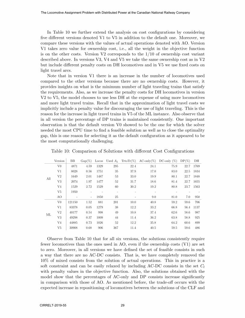
In Table 10 we further extend the analysis on cost configurations by consideringfive different versions denoted V1 to V5 in addition to the default one. Moreover, wecompare these versions with the values of actual operations denoted with AO. VersionV1 takes zero value for ownership cost, i.e., all the weight in the objective functionis on the other costs. Version V2 corresponds to the 1/10 of ownership cost variantdescribed above. In versions V3, V4 and V5 we take the same ownership cost as in V2but include different penalty costs on DH locomotives and in V5 we use fixed costs onlight travel arcs.

Note that in version V1 there is an increase in the number of locomotives usedcompared to the other versions because there are no ownership costs. However, itprovides insights on what is the minimum number of light traveling trains that satisfythe requirements. Also, as we increase the penalty costs for DH locomotives in versionV2 to V5, the model chooses to use less DH at the expense of using more locomotivesand more light travel trains. Recall that in the approximation of light travel costs weimplicitly include a penalty value for discouraging the use of light traveling. This is thereason for the increase in light travel trains in V5 of the ML instance. Also observe thatin all version the percentage of DP trains is maintained consistently. One importantobservation is that the default version V0 showed to be the one for which the solverneeded the most CPU time to find a feasible solution as well as to close the optimalitygap, this is one reason for selecting it as the default configuration as it appeared to bethe most computationally challenging.

Table 10: Comparison of Solutions with different Cost Configurations

Version BB Gap(%) Locos Used AL TrtoTr(%) AC-only(%) DC-only (%) DP(%) DH

All

V0 4871 4.59 1329 295 22.4 24.1 75.9 22.7 1769

V1 8028 0.56 1751 35 37.9 17.0 83.0 22.5 1834

V2 1649 2.01 1487 53 33.0 19.9 80.1 22.7 1848

V3 2074 1.97 1477 52 31.7 18.6 81.4 22.7 1655

V4 1529 2.72 1529 60 30.2 19.2 80.8 23.7 1563

V5 1950 - - - - - - - -

AO - - 1850 25 - 9.0 81.0 7.0 950

ML

V0 121150 1.52 881 201 10.0 40.8 59.2 59.6 706

V1 83378 0.05 1279 38 12.2 33.2 66.8 56.4 1137

V2 40177 0.54 998 49 10.8 37.4 62.6 58.6 987

V3 49298 0.37 1009 44 11.4 36.2 63.8 58.8 925

V4 44885 0.73 1026 52 12.2 35.8 64.2 60.6 899

V5 30908 0.68 906 367 11.4 40.5 59.5 59.6 486

Observe from Table 10 that for all six versions, the solutions consistently requirefewer locomotives than the ones used in AO, even if the ownership costs (V1) are setto zero. Moreover, in all versions we have defined the set of feasible consists in sucha way that there are no AC-DC consists. That is, we have completely removed the10% of mixed consists from the solution of actual operations. This in practice is asoft constraint and can be easily relaxed by including AC-DC consists in the set Cl

with penalty values in the objective function. Also, the solutions obtained with themodel show that the percentages of AC-only and DP consists increase significantlyin comparison with those of AO. As mentioned before, the trade-off occurs with theexpected increase in repositioning of locomotives between the solutions of the CLF and


CIRRELT-2019-55 29

the actual operations. This can be explained with the cyclic behavior requirements ofthe model and the foreign power modeling part that will be treated at the LRP-DPlevel.

Table 11: Comparison of Solutions with different Configurations for Extra DH

Extra DH Thr BB Gap(%) Locos Used AL Used AQ(%) AC-only (%) DC-only (%) DP(%) DH

All

no NA 23993 - - - - - - - -

yes 10 4871 4.59 1329 295 22.4 24.1 75.9 22.7 1769

yes 30 4025 4.70 1296 228 21.3 24.1 75.9 22.7 1995

yes 200 4806 4.25 1272 212 20.0 25.2 74.8 23.2 2231

ML

no NA 175704 6.22 973 328 8.7 36.5 63.5 54.6 453

yes 10 121150 1.52 881 201 10.0 40.8 59.2 59.6 706

yes 30 111197 1.09 859 190 8.7 42.3 57.7 59.9 796

yes 200 104781 0.95 856 179 8.3 41.2 58.8 60.3 797

Another parameter that we evaluate is the number of extra DH arcs. Recall that wecontrol how extra DH arcs are created depending on a threshold value on the numberof inbound or outbound trains at each intermediate station of a train route. This valueis denoted as Thr in Table 11. Thus, given the cost configuration of the model as weincrease the possibility of DH, the solution tends to have more DH locomotives in orderto reduce the number of locomotives used. However, this can be modified according tothe planning preferences and requirements.

Finally, the model can also be used to identify trade-offs when modifying the sizeof the locomotive fleet. For example, managers can receive insights on which types oflocomotives should be bought. In Table 12 we show two examples when +/- 20% oflocomotives are available. On the one hand, as the locomotive fleet becomes larger theenhanced model is easier to solve which can be exploited in a solution method basedon Lagrangean Relaxation. On the other hand, when the locomotive fleet is tightto satisfy train requirements the proposed Benders approach can be used to obtainfeasible solutions faster.

Table 12: Comparison of Solutions Considering Different Fleet Size

Fleet Size BB UB Locos DH Gap(%) N.Sols Used AL DP(%)

All

default 4871 14684483 1329 1769 4.59 6 295 23.23

-20% 7950 NA NA NA NA 0 NA NA

+20% 5129 14439899 1308 1735 3.52 18 250 24.98

ML

default 121150 11126320 881 706 1.52 116 201 59.58

-20% 96300 11333270 898 718 2.10 135 214 53.07

+20% 115418 11028619 872 697 1.15 144 202 60.07

6 Conclusions

The purpose of this study was to introduce, model and solve a general tactical-levelversion of the LAP in which the operation mode of the trains is part of the decision


30 CIRRELT-2019-55

process. In the problem definition we also incorporated several real-life aspects basedon the requirements and discussions with the Canadian National Railway Company,one of the largest railway companies in North America. To model the problem wepresented two ILP formulations that were computationally tested on realistic instances.The results of extensive computational experiments confirm the efficiency of variousenhancements on the CLF model when solved with a general-purpose solver yieldinggood solutions in reasonable time. Moreover the two versions of the Benders-basedalgorithm showed to significantly reduce the CPU time to obtain a first solution. Also,the decomposition structure seems well-suited for problem extensions, in particularthose including uncertainty in the parameters.

We also discussed the results obtained with the model and solution approach usingdifferent input parameters. Notoriously, even with an optimality gap of over 4%, theenhanced model provided solutions, under certain costs configurations, where approxi-mately 25% fewer locomotives are required than those used in actual operations. Thismajor reduction is a trade-off with the increase in repositioning locomotives in the net-work but also is partly explained by the fact that we are comparing at different levelsof decision. Thus, care should be taken to avoid misleading conclusions on solutionsthat could be more difficult to comply with at the operational level, especially afterwhen studying other extensions of the problem that will be the object of subsequentresearch, for example, concerning uncertainty. Nevertheless, given the results presentedin this article, we believe that the proposed model is well-suited to provide insights onlocomotive planning and that the potential for cost reduction is very significant.

References

[1] Y. Adulyasak, J.-F. Cordeau, and R. Jans. Benders decomposition for productionrouting under demand uncertainty. Operations Research, 63(4):851–867, 2015.

[2] R. K. Ahuja, J. Liu, J. B. Orlin, D. Sharma, and L. A. Shughart. Solving real-lifelocomotive-scheduling problems. Transportation Science, 39(4):503–517, 2005.

[3] R. K. Ahuja, T. L. Magnanti, and J. B. Orlin. Network Flows: Theory, Algorithms,and Applications. Prentice Hall, Englewood Cliffs, New Jersey, 1993.

[4] J. F. Benders. Partitioning procedures for solving mixed-variables programmingproblems. Numerische Mathematik, 4(1):238–252, 1962.

[5] M. Bodur and J. R. Luedtke. Mixed-integer rounding enhanced Benders decom-position for multiclass service-system staffing and scheduling with arrival rateuncertainty. Management Science, 63(7):2073–2091, 2016.

[6] B. Bouzaiene-Ayari, C. Cheng, S. Das, R. Fiorillo, and W. B. Powell. From singlecommodity to multiattribute models for locomotive optimization: A comparisonof optimal integer programming and approximate dynamic programming. Trans-portation Science, 50(2):366–389, 2016.

[7] J.-F. Cordeau, F. Soumis, and J. Desrosiers. A Benders decomposition ap-proach for the locomotive and car assignment problem. Transportation Science,34(2):133–149, 2000.


CIRRELT-2019-55 31

[8] J.-F. Cordeau, F. Soumis, and J. Desrosiers. Simultaneous assignment of locomo-tives and cars to passenger trains. Operations Research, 49(4):531–548, 2001.

[9] J.-F. Cordeau, P. Toth, and D. Vigo. A survey of optimization models for trainrouting and scheduling. Transportation Science, 32(4):380–404, 1998.

[10] S. Deveau. How long can trains go? National Post, 2011.

[11] M. Fischetti, I. Ljubic, and M. Sinnl. Redesigning Benders decomposition forlarge-scale facility location. Management Science, 63(7):2146–2162, 2017.

[12] M. Florian, G. Bushell, J. Ferland, G. Guerin, and L. Nastansky. The enginescheduling problem in a railway network. INFOR, 14:121–138, 1976.

[13] B. Jaumard and H. Tian. Multi-column generation model for the locomotive as-signment problem. In M. Goerigk and R. Werneck, editors, OpenAccess Series inInformatics (OASIcs). 16th Workshop on Algorithmic Approaches for Transporta-tion Modelling, Optimization, and Systems (ATMOS 2016). Schloss Dagstuhl–Leibniz-Zentrum fuer Informatik. Dagstuhl, Germany, 2016.

[14] T. L. Magnanti and R. T. Wong. Accelerating Benders decomposition: Algorith-mic enhancement and model selection criteria. Operations Research, 29(3):464–484, 1981.

[15] C. Ortiz-Astorquiza, I. Contreras, and G. Laporte. An exact algorithm for multi-level uncapacitated facility location. Transportation Science, 53:1085–1106, 2019.

[16] F. Piu, V. Kumar, and M. G. Speranza. Introducing a preliminary consists se-lection in the locomotive assignment problem. Transportation Research Part E:Logistics and Transportation Review, 82:217–237, 2015.

[17] F. Piu and M. G. Speranza. The locomotive assignment problem: A survey on op-timization models. International Transactions in Operational Research, 21(3):327–352, 2014.

[18] W. B. Powell, B. Bouzaiene-Ayari, C. Lawrence, C. Cheng, S. Das, and R. Fio-rillo. Locomotive planning at norfolk southern: An optimizing simulator usingapproximate dynamic programming. Interfaces, 44(6):567–578, 2014.

[19] RAC. Railway association of Canada, 2018.https://www.railcan.ca/101/delivering-canadas-amazing-products-to-the-world/.

[20] R. Rahmaniani, T. G. Crainic, M. Gendreau, and W. Rei. The Benders decompo-sition algorithm: A literature review. European Journal of Operational Research,259(3):801–817, 2017.

[21] B. Vaidyanathan, R. K. Ahuja, J. Liu, and L. A. Shughart. Real-life locomotiveplanning: New formulations and computational results. Transportation ResearchPart B: Methodological, 42(2):147–168, 2008.

[22] B. Vaidyanathan, R. K. Ahuja, and J. B. Orlin. The locomotive routing problem.Transportation Science, 42(4):492–507, 2008.


32 CIRRELT-2019-55

[23] K. Ziarati, F. F. Soumis, J. Desrosiers, S. Gelinas, and A. Saintonge. Locomotiveassignment with heterogeneous consists at CN north america. European Journalof Operational Research, 97(2):281–292, 1997.

[24] K. Ziarati, F. F. Soumis, J. Desrosiers, and M. M. Solomon. A branch-first, cut-second approach for locomotive assignment. Management Science, 8(45):1156–1168, 1999.

A Appendix: A Locomotive Flow-Based For-

mulation

Let xkl be the number of active locomotives of type k assigned to arc l ∈ AT ∪AC∪ADP

and ykl be the number of non-active locomotives of type k assigned to arc l ∈ A. Also,let zl = 1 if arc l ∈ AC ∪ AL is used and 0 otherwise. Similarly, vl = 1 if train loperates on DP mode or equivalently if the associated DP arc l ∈ ADP is used in thesolution. Binary variables acl and dcl take value 1 if train l ∈ AT is operated with aconsist formed of only AC or DC locomotives, respectively. Finally, ul are variablesto control a soft constraint that determines the total number of active axles per train.Note that although the xkl variables model the active locomotives on a train, theyare defined on a larger set. This definition becomes useful when modeling extra DHthrough train-to-train connections.

Now, let x be the vector of decision variables, the total cost Tot(x) can be writtenas

Tot(x) =∑k∈K

∑l∈AT

ckl xkl +

∑k∈K

∑l∈AC∪ADP

dkl (xkl + ykl ) +∑k∈K

∑l∈S

gk(xkl + ykl )

+∑k∈K

∑l∈AT∪ADH∪AG∪AL

dkl ykl +

∑l∈AR

pzl +∑l∈AL

blzl +∑l∈AT

ul + P (x),

where P (x) is a function associated with weights for penalties and preferences of solu-tion features such as mix AC-DC consists and DP among others. The operational costof assigning an active locomotive of type k to train l is denoted ckl and is modeled asa function of the track maintenance and fuel consumption costs. On the other hand,dkl varies depending on the arc l. For example, if l ∈ AT ∪ ADH , dkl corresponds tothe cost of DH a locomotive of type k using arc l whereas if l ∈ AL, dkl represents theunitary cost of light traveling a locomotive of type k on arc l. Fixed costs p and blrepresent the cost of activating an arc in the network. In the case of light travel arcs itcorresponds to the associated crew and fuel costs. The fixed cost p of busting a consistas well as the penalties and preferences are more subjective and depend on how muchweight the user wants to place on certain characteristics of the solution. Given the setsI[i] and O[i] of inbound and outbound arcs of node i ∈ N , respectively and E(l, i, j)the set of extra DH arcs between stations i and j associated with train route Rl, theLocomotive Flow-Based Formulation (LBF) can be expressed as


CIRRELT-2019-55 33

minimize Tot(x) (47)

subject to∑k∈K

hkxkl ≥ βltl(1− acl)+βAl tlacl − tlθlvl ∀ l ∈ AT (48)∑l∈I[i]

xkl =∑l∈O[i]

xkl ∀ i ∈ NA ∪ND, k ∈ K (49a)

∑l∈I[i]

ykl =∑l∈O[i]

ykl ∀ i ∈ NA ∪ND ∪NI , k ∈ K (49b)

∑l∈I[i]

(xkl + ykl ) =∑l∈O[i]

ykl ∀ i ∈ NR, k ∈ K (49c)

∑l∈I[i]

ykl =∑l∈O[i]

(xkl + ykl ) ∀ i ∈ NE ∪NDP , k ∈ K (49d)

∑k∈K

xkl∗ ≤ mDvl +mA(1− vl) ∀ l∗ = (i, j) ∈ AT , l ∈ ADP ∩ I[i] (50)∑k∈K

xkl +∑k∈K

∑l∗∈E(l,i,j)

ykl∗ ≤ mT ∀ l ∈ AT , i, j ∈ Rl (51)

∑k∈K

(xkl + ykl ) ≤ mT zl ∀ l ∈ AC (52)∑k∈K

ykl ≤ mT zl ∀ l ∈ AL (53)∑k∈K

(xkl + ykl ) ≤ mT vl ∀ l ∈ ADP (54)∑l∈O[i]:l∈AQ

zl ≤ 1 ∀ i ∈ NA (55)

∑l∈I[i]:l∈AQ

zl ≤ 1 ∀ i ∈ ND (56)

∑k∈K

xkl ≥ 2zl ∀ k ∈ K, l ∈ AQ (57)

zl ≤ 1− vl∗ ∀ (i, j) ∈ AT , l ∈ AQ ∩O[j], l∗ ∈ ADP ∩ I[i](58)∑

l∈I[i]:l /∈AE

vl + zl ≤ 1 ∀ i ∈ ND (59)

zl∗ ≤ 1− vl ∀ l∗ = (i, j) ∈ AE , l ∈ ADP ∩ I[j] (60)∑k∈K

xkl ≤ mA(1−∑

l∗∈AQ:l∗∈I[j]

zl∗) ∀ l = (i, j) ∈ AE (61)


34 CIRRELT-2019-55

∑k∈K

λkxkl − ul ≤ al ∀ l ∈ AT (62)∑l∈S

(xkl + ykl ) ≤ fk ∀ k ∈ K (63)∑k∈K:dpk=1

xkl ≥ 2vl ∀ k ∈ K, l ∈ ADP (64)

dcl ≤ 1− (1/mA)∑k∈AC

xkl ∀ l ∈ AT (65)

acl ≤ 1− (1/mA)∑

k∈DC

xkl ∀ l ∈ AT (66)

acl + dcl ≤ 1 ∀ l ∈ AT (67)

xkl ∈ Z+ ∀ l ∈ AT ∪AC ∪ADP , k ∈ K (68)

ykl ∈ Z+ ∀ l ∈ A, k ∈ K (69)

zl ∈ {0, 1} ∀ l ∈ AC ∪AL (70)

vl ∈ {0, 1} ∀ l ∈ ADP , (71)

acl, dcl ∈ {0, 1} ∀ l ∈ AT , (72)

where mA, mT and mD are the maximum number of active, total and DP locomo-tives allowed on each train. Constraints (48) ensure that the horsepower requirementfor every train is met. Note that depending on the selection of DP mode or AC-onlyconsists the HPT of the train may vary affecting the overall HP required and thusthe number of locomotives assigned. Equations (49a)–(49d) are flow conservation con-straints. Constraints (50) limit the maximum number of pulling locomotives allowedper train for both DP and conventional modes while constraints (51) limit the max-imum number of total locomotives per train. Note that when the set E(l, i, j) = {l}we are in the particular case of no extra DH at intermediate stations. The sets ofconstraints (52), (53) and (54) link the flow variables with the binary variables andlimit the maximum number of locomotives on AC , AL and ADP , respectively. Con-straints (55) and (56) establish that at most one train-to-train connection is allowedat each train arrival or train departure node while (57) guarantee that a train-to-trainconnection is only used for reusing consists i.e. only for consists of size greater thanone. Constraints (58) consider that when a train operates on DP mode, a train-to-trainconnection at the arrival station is not possible. Similarly, constraints (59) ensure thatif a train-to-train connection occurs at a train-departure node, the DP mode cannotbe used on that train and vice-versa. Note that in (59) we do not include the variableassociated with ground-departure arcs. This means that both a ground-departure anda train-to-train arc could be active, which allows to add DH locomotives in a train-to-train connection. On the other hand, constraints (60) guarantee that each traineither operates on DP or conventional mode. The set of constraints (61) ensures thatif there is a train-to-train connection no new active locomotives can be added to theconsist. Constraints (62) control the maximum number of active axles per train andconstraints (63) impose the number of available locomotives by type. Constraints (64)ensure that at least two DP equipped locomotives are assigned if the train runs on DPmode and finally, constraints (65) to (67) describe the use of AC-only, DC-only and


CIRRELT-2019-55 35

mixed DC-AC consists.In addition, other operational requirements are included by fixing variables. For

example, we set xkl = 0 if train l is a mainline train (l ∈ ML) and locomotive typek belongs to the set of low HP locomotives. That is, low HP types are not allowedto operate mainline trains mainly because of reliability. Also, as mentioned before weforce some train-to-train connections given by a set of rules provided by the railway.This is accomplished by setting zl = 1 for the corresponding l ∈ AQ. Finally, when atrain is heavier or longer than threshold values to be operating on conventional mode,we enforce those trains on DP mode by setting vl = 1.


36 CIRRELT-2019-55

the locomotive assignment problem with distributed power … · 2019-11-28 · the locomotive...

Documents