the log-gamma-logistic regression model: estimation

The Log-gamma-logistic Regression Model:Estimation, Sensibility and Residual Analysis

Elizabeth M. Hashimoto

Departamento Academico de Matematica,Universidade Tecnologica Federal do Parana

Londrina, [email protected]

Edwin M.M. Ortega∗

Departamento de Ciencias Exatas,Universidade de Sao Paulo

Piracicaba, [email protected]

Gauss M. Cordeiro

Departamento de Estatıstica,Universidade Federal de Pernambuco,

Recife, [email protected]

G.G. Hamedani

Department of Mathematics, Statistics and Computer Science,Marquette University, Milwaukee, [email protected]

In this paper, we formulate and develop a log-linear model using a new distribution called the log-gamma-logistic. We show that the new regression model can be applied to censored data since it represents a para-metric family of models that includes as sub-models several widely-known regression models and thereforecan be used more effectively in the analysis of survival data. We obtain maximum likelihood estimates of themodel parameters by considering censored data and evaluate local influence on the estimates of the parametersby taking different perturbation schemes. Some global-influence measurements are also investigated. Further,for different parameter settings, sample sizes and censoring percentages, various simulations are performed.In addition, the empirical distributions of some modified residuals are displayed and compared with the stan-dard normal distribution. These studies suggest that the residual analysis usually performed in normal linearregression models can be extended to modified deviance residuals in the proposed regression model applied tocensored data. We demonstrate that our extended regression model is very useful to the analysis of real dataand may give more realistic fits than other special regression models.

Keywords: Censored data; gamma-log-logistic distribution; regression model; residual analysis; sensitivityanalysis.

∗Corresponding author.

Journal of Statistical Theory and Applications, Vol. 16, No. 4 (December 2017) 547–564___________________________________________________________________________________________________________

547

Received 27 February 2016

Accepted 18 February 2017

Copyright © 2017, the Authors. Published by Atlantis Press.This is an open access article under the CC BY-NC license (http://creativecommons.org/licenses/by-nc/4.0/).

1. Introduction

The log-logistic distribution is widely used in survival analysis and it is an alternative to the Weibulland lognormal distributions since it presents a hazard rate function (hrf) that increases, reaches apeak after some finite period and then declines gradually. The properties of the log-logistic distri-bution make it an attractive alternative to the log-normal and Weibull distributions in the analysisof survival data (Collet, 2003). Recently, for any continuous baseline G distribution, Zografos andBalakrishnan (2009) proposed a generalized gamma-generated distribution with an extra positiveparameter. A three-parameter continuous model called the gamma-log-logistic (GLL) distribution,which extends the log-logistic model, investigated by Ramos et al. (2013).

One way to study the effects of the explanatory variables on the lifetime or survival time isthrough a regression location-scale model, also known as the accelerated lifetime model. Thesemodels consider that the response variable belongs to a family of distributions characterized by aparameter location and scale parameter. However, for the case of parametric models, it is consideredthat the lifetime follows a continuous distribution. Regression models can be proposed in differentforms in survival analysis. Among them, the location-scale regression model (Lawless, 2003) isdistinguished and it is frequently used in clinical trials. So, in the context of survival analysis, somedistributions have been used as an alternative to analyze censored data.

In this paper, we define a location-scale regression model using the GLL distribuition called thelog-gamma-logistic (LGL) regression model. We consider a classic analysis for the LGL regres-sion model. The inferential part was carried out using the asymptotic distribution of the maximumlikelihood estimators (MLEs), which in situations when the sample size is small, may present dif-ficult results to be justified. As an alternative to classic analysis, we explore the use of bootstrapmethod for survival time analysis as a feasible alternative. After modeling, it is important to checksome model assumptions as well as to conduct a robustness study in order to detect influential orextreme observations that can cause distortions in the results of the analysis. We develops a similarmethodology to detect influential subjects in LGL regression models with censored data.

We compare two residuals to assess departures from the error assumptions and to detect outlyingobservations in LGL regression models with censored observations. For different parameter settings,sample sizes and censoring percentages, various simulation studies are performed and the empiricaldistribution of each residual is displayed and compared with the standard normal distribution.

The rest of the paper is outlined as follows. In Section 2, we consider a brief study on the GLLdistribution and present certain the characterizations of LGL distribution. In Section 3, we define aLGL regression model of location-scale form, in addition to the MLEs, bootstrap method and theresults from various simulation studies are explored. In Section 4, we use several diagnostic mea-sures considering three perturbation schemes, case-deletion and the generalized leverage in LGLregression models with censored observations. Section 5 deals with the definition and discussion ofthe residuals and presents and comments the results from various simulation studies. In Section 6,a real data set is analyzed and some conclusion are addressed in Section 7.

2. The log-gamma-logistic distribution

Many papers have been published on the log-logistic (LL) distribution, such as: Shoukri et al.(1988), who studied this distribution to describe phenomena involving precipitation in Canada;Shayan et al. (2011), who proposed LL regression with four parameters that allows description offailure rate data with bathtub distribution; Santana et al. (2012), who presented a generalization of


548

the LL distribution and its properties; and Zare et al. (2012), who used the LL distribution to analyzedata on breast cancer patients in the southern region of Iran. The probability density function (pdf)and cumulative distribution function (cdf) of the LL distribution are given by

g(t) =α

λ α tα−1[

1+( t

λ

)α]−2

and G(t) = 1−[

1+( t

λ

)α]−1

, (2.1)

respectively, where λ > 0 is the scale parameter and α > 0 is the shape parameter. From the workscited above, it can be noted that the LL distribution has been widely used in data analysis to describenatural phenomena and to predict future events, as is the case of water movement in the oceans.However, in some situations, the observed data have uncommon behavior, so the LL distributionis not suitable to describe and predict the phenomenon of interest. Recent developments have beenmade to define new generated families to control skewness and kurtosis through the tail weights andprovide great flexibility in modeling skewed data in practice, the generators pioneered by Eugeneet al. (2002), Cordeiro and de Castro (2011) and Alexander et al. (2012).

Recently, Zografos and Balakrishnan (2009) and Ristic and Balakrishnan (2012) proposed afamily of univariate distributions generated by gamma random variables. For any baseline cdf G(t),they defined the gamma-G distribution with pdf f (t) and cdf F(t) by

f (t) =1

Γ(ϕ)− log[1−G(t)]ϕ−1 g(t) (2.2)

and

F(t) =γ (ϕ ,− log [1−G(t)])

Γ(ϕ)=

1Γ(ϕ)

∫ − log[1−G(t)]

0uϕ−1e−udu,

respectively, for ϕ > 0, where g(t) = dG(t)/dt, Γ(a) =∫ ∞

0 ua−1 e−udu is the gamma function, andγ(a,z) =

∫ z0 ua−1 e−udu is the incomplete gamma function. The gamma-G distribution has the same

parameters of the G distribution plus an additional shape parameter ϕ > 0. Each new gamma-Gdistribution can be obtained from a specified G distribution. For ϕ = 1, the G distribution is a basicexemplar of the gamma-G distribution with a continuous crossover towards cases with differentshapes (for example, a particular combination of skewness and kurtosis).

Thus, the GLL distribution, proposed by Ramos et al. (2013) is obtained by inserting (2.1) inequation (2.2). So, we have

f (t) =α

λ αΓ(ϕ)tα−1

[1+( t

λ

)α]−2log[

1+( t

λ

)α]ϕ−1

, t > 0,

where ϕ > 0 and α > 0 are shape parameters and λ > 0 is a scale parameter.For ϕ = 1, we obtain the LL distribution. Like the LL and GLL distributions can be employed

in engineering and can be used to model reliability in survival problems. Plots of the GLL densityfunction for selected parameter values are displayed in Figure 1a. Plots of the GLL hrf for someparameter values are displayed in Figure 1b. The new hrf can have four types of shapes: increasing,decreasing, bathtub and unimodal.

To obtain a distribution that belongs to the location-scale class of models, we consider the trans-formation of the random variable Y = log(T ). Thus, setting α = 1/σ and λ = exp(µ), the pdf of Y


549

(a) (b)

0 1 2 3 4

0.0

0.5

1.0

1.5

2.0

t

f(t)

GLL(φ = 1, λ = 0.6, α = 3)GLL(φ = 0.5, λ = 1, α = 0.5)GLL(φ = 1.5, λ = 2.5, α = 9)GLL(φ = 2, λ = 0.3, α = 1)GLL(φ = 3, λ = 1.5, α = 4)GLL(φ = 0.5, λ = 2, α = 2.5)

0 1 2 3 4 5

01

23

4

t

h(t)

GLL(φ = 0.5, λ = 1, α = 3)GLL(φ = 0.4, λ = 2, α = 0.6)GLL(φ = 3, λ = 1, α = 6.5)GLL(φ = 0.3, λ = 0.8, α = 2.9)

Fig. 1. (a) Plots of the GLL pdf for some parameter values. (b) Plots of the GLL hrf for some parameter values.

is given by

f (y) =1

σΓ(ϕ)exp(

y−µσ

)[1+ exp

(y−µ

σ

)]−2log[

1+ exp(

y−µσ

)]ϕ−1

, −∞ < y < ∞,(2.3)

where ϕ > 0, σ > 0 and −∞ < µ < ∞. Therefore, Y is a random variable having the log-gammalogistic (LGL) distribution. Plots of the pdf (2.3) for selected parameter values are given in Figure2. These plots show great flexibility for different values of the shape parameter ϕ with µ = 0 andσ = 1. Thus,

if T ∼ GLL(ϕ ,λ ,α) then Y = log(T )∼ LGL(ϕ ,µ,σ).

Moreover, the survival function corresponding to (2.3) is

S(y) = 1− 1Γ(ϕ)

γ(

log[

1+ exp(

y−µσ

)],ϕ).

On the other hand, we define the standardized random variable Z = (Y − µ)/σ with densityfunction

−10 −5 0 5 10

0.00

0.05

0.10

0.15

0.20

0.25

0.30

y

f(y)

φ = 0.2φ = 0.5φ = 1φ = 1.5φ = 2φ = 3

Fig. 2. Some shapes of the pdf of the LGL distribution.


550

π(z;ϕ) =1

Γ(ϕ)exp(z) [1+ exp(z)]−2 log [1+ exp(z)]ϕ−1 , −∞ < z < ∞. (2.4)

The case ϕ = 1 refers to the logistic distribution.The rth moment of the LGL distribution is given by

µ ′r =

1Γ(ϕ)

r

∑i=0

(ri

)σ i µr−i

∫ 1

0

[log(

1−uu

)]i[log(

1u

)]ϕ−1

du, (2.5)

where u =[1+ exp

( y−µσ)]−1

.From equation (2.5) it is possible to determine the mean and variance of the LGL distribution.

2.1. Characterizations of LGL Distribution

We emphasize the importance of characterizing the new model LGL. Characterizations of the dis-tributions provide conditions under which the underlying distribution is indeed that particular dis-tribution of interest.

2.1.1. Characterizations based on truncated moments

In this subsection we present characterizations of LGL distribution in terms of a simple relationshipbetween two truncated moments.

Proposition 2.1. Let Y : Ω → R be a continuous random variable and let

h(y) = g(y)[

1+ exp(

y−µσ

)]−1

and g(y) =

log[

1+ exp(

y−µσ

)]1−ϕ, for y ∈ R.

Then, pdf of Y is (3) if and only if the function η defined in Theorem A.1 (see Appendix) has theform

η (y) = 2[

1+ exp(

y−µσ

)], y ∈ R. (2.6)

Proof. Let Y have pdf (2.6), then

[1−F (y)]E [h(Y ) | Y ≥ y] =1

2Γ(ϕ)

[1+ exp

(y−µ

σ

)]−2

, y ∈ R ,

and

[1−F (y)]E [g(Y ) | Y ≥ y] =1

Γ(ϕ)

[1+ exp

(y−µ

σ

)]−1

, y ∈ R ,

and finally,


551

η (y)h(y)−g(y) = g(y)> 0 for y ∈ R.

Conversely, if η (y) is given by (2.6), then

s′ (y) =η ′ (y)h(y)

η (y)h(y)−g(y)=

2σ

exp(

y−µσ

)[1+ exp

(y−µ

σ

)]−1

,

from which we obtain

s(y) = 2log[

1+ exp(

y−µσ

)], y ∈ R .

Now, in view of Theorem A.1 , Y has pdf (3).

Corollary 2.1. Let Y : Ω → R be a continuous random variable and let h be as in Proposition 1.1.Then, pdf of Y is (3) if and only if there exist functions g and η defined in Theorem A.1 satisfyingthe following differential equation

s′ (y) =η ′ (y)h(y)

η (y)h(y)−g(y)=

2σ

exp(

y−µσ

)[1+ exp

(y−µ

σ

)]−1

, y ∈ R. (2.7)

Remarks. (a) The general solution of the differential equation (2.7) is

η (y) =[

1+ exp(

y−µσ

)]2[−∫ 2

σexp(

y−µσ

)[1+ exp

(y−µ

σ

)]−3

(h(y))−1 g(y)dx+D

],

for y ∈R, where D is a constant. One set of function (h,g,η) satisfying the above equation is givenin Proposition 1.1 for D = 0.

(b) Clearly there are other triple of functions (h,g,η) satisfying the conditions of Theorem A.1.We presented one such pair in Proposition 1.1.

2.1.2. Characterization based on hazard function

The hazard function, ζF , of a twice differentiable distribution function, F , satisfies the first orderdifferential equation

ζ ′F (y)

ζF (y)−ζF (y) = q(y) ,

where q(y) is an appropriate integrable function. Although this differential equation has an obviousform since


552

ζ ′F (y)

ζF (y)−ζF (y) =

f ′ (y)f (y)

, (2.8)

for many univariate continuous distributions (2.8) seems to be the only differential equation in termsof the hazard function. The goal of the characterization based on hazard function is to establish adifferential equation in terms of hazard function, which has as simple form as possible and is not ofthe trivial form (2.8). Here, we present a characterization of the of LGL model based on a nontrivialdifferential equation in terms of the hazard function.

Proposition 2.2. Let Y : Ω → R be a continuous random variable. Then, Y has pdf (3) if and onlyif its hazard function ζF satisfies the differential equation

ζ ′F (y)−

1σ

ζF (y) = exp(

y−µσ

)ddx

B(y) , y ∈ R (2.9)

where

B(y) =

[1+ exp

( y−µσ)]−2

log[1+ exp

( y−µσ)]ϕ−1

Γ(ϕ)− γ(log[1+ exp

( y−µσ)],ϕ) .

Proof. If Y has pdf (3), then clearly (2.9) holds. Now, if (2.9) holds, then after multiplying bothsides of (2.9) by exp

−( y−µ

σ)

, we arrive at

ddy

exp−(

y−µσ

)ζF (y)

=

ddy

B(y) ,

from which we have

ζF (y) =f (y)

1−F (y)= exp

(y−µ

σ

)B(y) , y ∈ R. (2.10)

Integrating both sides of (2.10) from −∞ to y, we have

F (x) =1

Γ(ϕ)γ(

log[

1+ exp(

y−µσ

)],ϕ), y ∈ R.

3. The LGL regression models with censored data

In practice there are many situations where the response variable yi is influenced by one or moreexplanatory variables or covariates, and can be related to treatments, intrinsic traits of sample units,exogenous variables, interactions or time-dependent variables, among others. Let xi =(xi1, . . . ,xip)

⊤

be the explanatory variable vector associated with the ith response variable yi for i = 1, . . . ,n.


553

For the first time, we construct a linear regression model for the response variable yi based onthe LGL distribution given by

yi = x⊤i β +σzi, i = 1, . . . ,n, (3.1)

where the random error zi has the density function (2.4), β = (β1, . . . ,βp)⊤, σ > 0 and ϕ > 0

are unknown scale parameters and xi is the vector of explanatory variables modeling the locationparameter µi = x⊤i β . Hence, the location parameter vector µ = (µ1, . . . ,µn)

⊤ of the LGL model hasa linear structure µ = xβ , where x = (x1, . . . ,xn)

⊤ is a known model matrix. The logistic regressionmodel is defined by (3.1) with ϕ = 1.

Consider a sample (y1,x1), . . . ,(yn,xn) of n independent observations, where each randomresponse is defined by yi = minlog(ti), log(ci). We consider non-informative censoring suchthat the observed lifetimes and censoring times are independent. The log-likelihood function forθ reduces to

l(θ) =−r log(σ)− r log[Γ(ϕ)]+1σ

n

∑i=1

δi(yi −x⊤i β )−2n

∑i=1

δi log [1+

exp(

yi −x⊤i βσ

)]+(ϕ −1)

n

∑i=1

δi log

log[

1+ exp(

yi −x⊤i βσ

)]+

n

∑i=1

(1−δi) log

1− 1Γ(ϕ)

γ(

log[

1+ exp(

yi −x⊤i βσ

)],ϕ)

, (3.2)

where θ = (ϕ ,σ ,β⊤)⊤ is the vector of unknown parameters, r is the number of non-censoredobservations.

The MLE θ of θ can be obtained by maximizing the log-likelihood function (3.2). We use thematrix programming language Ox (MaxBFGS function) (see Doornik, 2007) to calculate θ . Initialvalues for β and σ are taken from the fit of the logistic regression model with ϕ = 1.

From the fitted model (3.1), the survival function for yi can be estimated by

S(y; ϕ , σ , β⊤) = 1− 1

Γ(ϕ)γ

(log

[1+ exp

(y−x⊤β

σ

)], ϕ

).

Under general regularity conditions, the asymptotic distribution of (θ −θ) is multivariate nor-mal Np+2(0,K(θ)−1), where K(θ) is the expected information matrix. The asymptotic covariancematrix K(θ)−1 of θ can be approximated by the inverse of the (p+ 2)× (p+ 2) observed infor-mation matrix J(θ) and then the inference on the parameter vector θ can be based on the normalapproximation Np+2(0,J(θ)−1) for θ . The multivariate normal Np+2(0,J(θ)−1) distribution can beused to construct approximate confidence regions for some parameters in θ and for the hazard andsurvival functions. In fact, a 100(1−α∗)% asymptotic confidence interval for each parameter θq isgiven by

ACIq =

(θq − zα∗/2

√−Jq,q, θq + zα∗/2

√−Jq,q

),

where −Jq,q represents the qth diagonal element of the inverse of the estimated observed infor-mation matrix J(θ)−1 and zα∗/2 is the quantile 1−α∗/2 of the standard normal distribution. The


554

likelihood ratio (LR) statistic can be used to discriminate between the LGL and logistic regressionmodels since they are nested models. In this case, the hypotheses to be tested are H0 : ϕ = 1 versusH1 : H0 is not true, and the LR statistic reduces to w = 2l(θ)− l(θ), where θ is the MLE of θunder H0. The null hypothesis is rejected if w > χ2

1−α∗(1), where χ21−α∗(1) is the quantile of the

chi-square distribution with two degrees of freedom.

3.1. Bootstrap re-sampling method

The bootstrap re-sampling method was proposed by Efron (1979). The method considers theobserved sample as if it represents the population. From the information obtained from the sam-ple, B bootstrap samples of similar size to that of the observed sample are generated, from which itis possible to estimate various characteristics of the population, such as mean, variance, percentilesand so on.

According to the literature, the re-sampling method may be non-parametric or parametric. Inthis study, the non-parametric bootstrap method is addressed, according to which the distributionfunction F can be estimated by the empirical distribution F (Hashimoto et al., 2013).

Let T=(T1, . . . ,Tn) be an observed random sample and F be the empirical distribution of T. Thus,a bootstrap sample T∗ is constructed by re-sampling with replacement of n elements of the sampleT. For the B bootstrap samples generated, T ∗

1 , . . . ,T∗

B , the bootstrap replication of the parameter ofinterest for the bth sample is

θ ∗b = s(T ∗

b ),

i.e., the value of θ for sample T ∗b , b = 1, . . . ,B.

The bootstrap estimator of the standard error (Efron and Tibshirani, 1993) is the standard devi-ation of these bootstrap samples given by

EPB =

[1

(B−1)

B

∑b=1

(θ ∗

b − θB)2]1/2

,

where θB = 1B ∑B

b=1 θ ∗b . Note that B is the number of bootstrap generated samples. According to

Efron and Tibshirani (1993), assuming B ≥ 200, it is generally sufficient to present good results todetermine the bootstrap estimates. However, to achieve greater accuracy, a reasonably high B valuemust be considered. We describe the bias corrected and accelerated (BCa) method for constructingapproximated confidence intervals based on the bootstrap re-sampling method.

4. Sensitivity analysis

4.1. Global influence

A first tool to perform sensitivity analysis, as stated before, is by means of global influence startingfrom case-deletion. Case-deletion is a common approach to study the effect of dropping the ith casefrom the data set. A global influence measure considered by Xie and Wei (2007) is a generalizationof Cook distance, which is defined as a standardized norm of θ (i)− θ , and it is given by

GDi(θ) = (θ (i)− θ)⊤[L(θ)

](θ (i)− θ), (4.1)

where L(θ) is the observed information matrix.


555

Another measure to evaluate the influence of a case is presented by Cook and Weisberg (1982).This measure is called the likelihood distance and considers the difference between θ (i) and θ . Thus,the likelihood distance is given by

LDi(θ) = 2[l(θ)− l(θ (i))

], (4.2)

where l(θ) is the value of the logarithm of the likelihood function for the full sample and l(θ (i)) isthe value of the logarithm of the likelihood function for the sample excluding the ith observation.

4.2. Local influence

This approach is suggested by Cook (1986), where instead of removing observations, weights aregiven to them. Local influence calculation can be carried out for model (3.1). If likelihood displace-ment LD(ω) = 2l(θ)− l(θω ) is used, where θω denotes the MLE under the perturbed model,the normal curvature for θ at the direction d,∥ d ∥= 1, is given by Cd(θ) = 2|d⊤∆⊤[L(θ)]−1∆d|,where ∆ is a (p+2)n matrix that depends on the perturbation scheme, whose elements are given by∆vi = ∂ 2l(θ |ω)/∂θv∂ωi, i = 1,2, . . . ,n and v = 1,2, . . . , p+2, evaluated at θ and ω0, where ω0 isthe no perturbation vector.

We can also calculate normal curvatures Cd(ϕ), Cd(σ) and Cd(β ) to perform various index plots,for instance, the index plot of dmax, the eigenvector corresponding to Cdmax , the largest eigenvalue ofthe matrix B =−∆⊤[L(θ)]−1∆ and the index plots of Cdi(ϕ), Cdi(σ) and Cdi(β ), named total localinfluence (see, for example, Lesaffre and Verbeke, 1998), where di denotes an n×1 vector of zeroswith one at the ith position. Thus, the curvature at direction di takes the form Ci = 2|∆⊤

i[L(θ)

]−1∆i|,where ∆⊤

i denotes the ith row of ∆. It is customary to point out those cases such that Ci ≥ 2C, whereC = 1

n ∑ni=1Ci.

Next, we calculate, for three perturbation schemes (case-weight perturbation, response pertur-bation, explanatory variable perturbation), the matrix

∆ =(

∆vi

)[(p+2)×n

] =(∂ 2l(θ |ω)

∂θv∂ωi

)[(p+2)×n

],where v = 1,2, . . . , p+ 2 and i = 1,2, . . . ,n, considering the model defined in (3.1) and its log-likelihood function given by (3.2).

5. Residual analysis

In this section, we compare two residuals to assess departures from the error assumptions and todetect outliers in the LGL regression model with censored observations. In the literature, variousresiduals, were investigated, for example, Collett (2003), Weisberg (2005) and Colosimo and Giolo(2006). In the context of survival analysis, the deviance residuals have been more widely usedbecause they take into account the information of censored times (Silva et al., 2011). These residualscan also be used for the log-logistic regression model, which is a special case of the LGL regressionmodel. Thus, the plot of the deviance residuals versus the observed times provides a way to verifythe adequacy of the fitted model and to detect atypical observations.


556

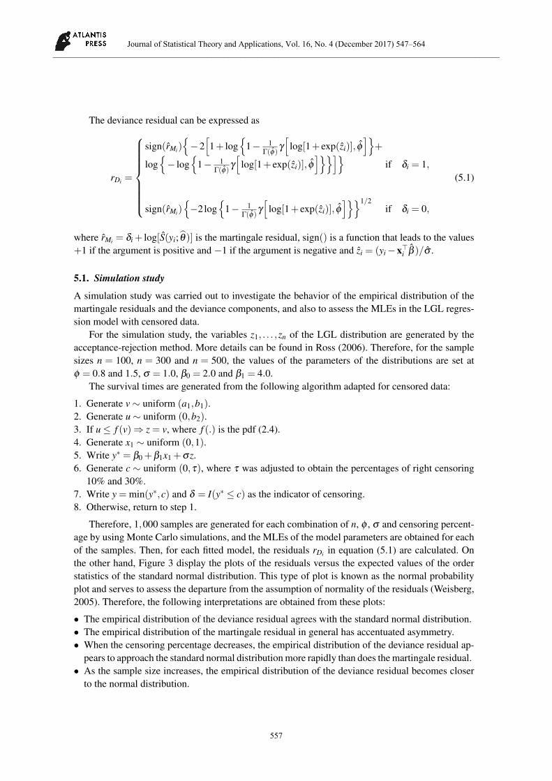
The deviance residual can be expressed as

rDi =

sign(rMi)−2[1+ log

1− 1

Γ(ϕ)γ[

log[1+ exp(zi)], ϕ]

+

log− log

1− 1

Γ(ϕ)γ[

log[1+ exp(zi)], ϕ]]

if δi = 1,

sign(rMi)−2log

1− 1

Γ(ϕ)γ[

log[1+ exp(zi)], ϕ]1/2

if δi = 0,

(5.1)

where rMi = δi + log[S(yi; θ)] is the martingale residual, sign() is a function that leads to the values+1 if the argument is positive and −1 if the argument is negative and zi = (yi −x⊤i β )/σ .

5.1. Simulation study

A simulation study was carried out to investigate the behavior of the empirical distribution of themartingale residuals and the deviance components, and also to assess the MLEs in the LGL regres-sion model with censored data.

For the simulation study, the variables z1, . . . ,zn of the LGL distribution are generated by theacceptance-rejection method. More details can be found in Ross (2006). Therefore, for the samplesizes n = 100, n = 300 and n = 500, the values of the parameters of the distributions are set atϕ = 0.8 and 1.5, σ = 1.0, β0 = 2.0 and β1 = 4.0.

The survival times are generated from the following algorithm adapted for censored data:

1. Generate v ∼ uniform (a1,b1).2. Generate u ∼ uniform (0,b2).3. If u ≤ f (v)⇒ z = v, where f (.) is the pdf (2.4).4. Generate x1 ∼ uniform (0,1).5. Write y∗ = β0 +β1x1 +σz.6. Generate c ∼ uniform (0,τ), where τ was adjusted to obtain the percentages of right censoring

10% and 30%.7. Write y = min(y∗,c) and δ = I(y∗ ≤ c) as the indicator of censoring.8. Otherwise, return to step 1.

Therefore, 1,000 samples are generated for each combination of n, ϕ , σ and censoring percent-age by using Monte Carlo simulations, and the MLEs of the model parameters are obtained for eachof the samples. Then, for each fitted model, the residuals rDi in equation (5.1) are calculated. Onthe other hand, Figure 3 display the plots of the residuals versus the expected values of the orderstatistics of the standard normal distribution. This type of plot is known as the normal probabilityplot and serves to assess the departure from the assumption of normality of the residuals (Weisberg,2005). Therefore, the following interpretations are obtained from these plots:

• The empirical distribution of the deviance residual agrees with the standard normal distribution.• The empirical distribution of the martingale residual in general has accentuated asymmetry.• When the censoring percentage decreases, the empirical distribution of the deviance residual ap-

pears to approach the standard normal distribution more rapidly than does the martingale residual.• As the sample size increases, the empirical distribution of the deviance residual becomes closer

to the normal distribution.


557

−2 −1 0 1 2

−20

12

3

Censored 0% Sample n=100

Standard normal quantiles

r Di

−2 −1 0 1 2

−20

12

3



r Di

−2 −1 0 1 2

−20

12

3



r Di

−2 −1 0 1 2

−20

12

3

Sample n=300


r Di

−2 −1 0 1 2

−20

12

3

Sample n=300


r Di

−2 −1 0 1 2

−20

12

3

Sample n=300


r Di

−3 −2 −1 0 1 2 3

−20

12

3

Sample n=500


r Di

−3 −2 −1 0 1 2 3

−20

12

3

Sample n=500


r Di

−3 −2 −1 0 1 2 3

−20

12

3

Sample n=500


r Di

Fig. 3. QQ-plot for the deviance residual (rDi) of the LGL regression model with ϕ = 0.8.

6. Application

To illustrate the application of the LGL regression model, we use a data set of Lee and Wang(2003). The data set refers to a study of patients diagnosed with acute myeloid leukemia (AML),where the objective was to determine factors associated with the lifetime of these patients. Thus, itwas observed that 30 patient lifetimes and possible prognostic factors:

• x1: Age (0= age of the patient < 50 years, 1= age of the patient ≥ 50 years);• x2: Cellularity (0= cellularity of marrow clot section is 100%, 1=otherwise).

First, to verify the behavior of the AML data, we construct the Kaplan-Meier and the TTT curve(Aarset, 1987) displayed in Figure 4. From these plots, we note that the TTT-plot indicates thatthe lifetime of patients has a unimodal failure rate (Figure 4a), which justifies the LL distribution.

(a) (b) (c)

0.0 0.2 0.4 0.6 0.8 1.0

0.0

0.2

0.4

0.6

0.8

1.0

i/n

TT

T

0 10 20 30 40

0.0

0.2

0.4

0.6

0.8

1.0

Time

Sur

viva

l fun

ctio

n es

timat

ed

0 10 20 30 40

0.0

0.4

0.8

Time

Sur

viva

l fun

ctio

n es

timat

ed

Age less than 50 yearsAge than equal to 50 years

0 10 20 30 40

0.0

0.4

0.8

Time

Sur

viva

l fun

ctio

n es

timat

ed

Cellularity 100%Cellurity less than 100%

Fig. 4. (a) TTT-plot. Survival curve estimate by Kaplan-Meier method for the: (b) lifetime. (c) explanatory variable (ageand cellularity).


558

Table 1. MLEs and non-parametric bootstrap estimates for the parameters of the regression model fitted to the AML data.

MLEs Non-parametric bootstrapParameter Estimate S.E. p-value Estimate S.E. 95% C.I. BCa

ϕ 5.918 4.529 – 5.069 0.910 (4.591, 7.940)σ 0.397 0.172 – 0.389 0.041 (0.333, 0.465)β0 1.053 0.992 0.288 1.195 0.388 (0.431, 1.597)β1 -1.092 0.338 0.001 -1.071 0.330 (-1.582, -0.494)β2 -0.315 0.338 0.351 -0.315 0.336 (-0.810, 0.283)

Moreover, the time does not present a level above zero, as shown in Figure 4b. On the other hand,we have evidence that only the age of the patients have an influence on lifetime (Figure 4c). Thus,accordance whit is observed in Figure 4, we consider the following model

yi = β0 +β1x1i +β2x2i +σzi, i = 1, . . . ,30,

where yi = log(ti) denotes the logarithm of lifetime.To maximize the log-likelihood function (3.2) and thus obtain the MLEs of the parameters of the

proposed model, we use the subroutine MaxBGFS of the matrix programming language Ox version(7.00) with initial values ϕ = 1.0, σ = 0.760, β0 = 4.880, β1 = -0.153 and β2 = 0.026. Thesevalues are obtained from the fit of the logistic regression model with censored data using the R

software version (2.15.1).Thus, in Table 1 we provide the parameter estimates, standard errors and significance of the

MLEs and non-parametric bootstrap estimates. The figures in this table indicate that the estimatesby the two methods are very similar, and then there is evidence that the presence of the only covariatex1 (age) is significant at 5% level of significance.

Further, we calculate the maximum unrestricted and restricted log-likelihoods and the likeli-hood ratio (LR) statistics for testing a special model. For example, the LR statistic for testing thehypotheses H0: ϕ = 1 versus H1: H0 is not true, i.e., to compare the LGL and logistic regressionmodels, is w = 2(−35.548+37.540) = 3.924 (p-value=0.048), which yields favorable indicationstoward to the LGL regression model.

The next step is to detect possible influential points in the LGL regression model. The mea-surements of global and local influence are calculated using the matrix programming language Ox

version 7.00.The generalized Cook’s distance (4.1) and likelihood distance (4.2) are given in Figure 5. These

plots indicate that the points ♯8, ♯17, ♯18 and ♯30 are possible influential observations.As for the plots of local influence, considering perturbations of cases (Cdmax = 1.1291) and the

logarithm of lifetime perturbation (Cdmax = 0.7453), it is noted that the cases ♯5, ♯7, ♯8, ♯17, ♯18 and♯30 can be considered as possible influential observations, as illustrated in Figure 6.

Also, Figure 7a indicates the deviance residuals. It can be noted that these residuals are random-ized around zero, indicating the suitability of the model for analyzing the lifespan data of patientswith AML.

Therefore, the sensitivity analysis (global influence and local influence) and the residual analysisdetected that the influential observations are ♯17, ♯18 and ♯30, which appeared more frequently.


559

(a) (b)

0 5 10 15 20 25 30

0.00.2

0.40.6

Index

|Gen

eralize

d Coo

k dist

ance

|

8

17

0 5 10 15 20 25 30

01

23

45

Index

|Like

lihoo

d dist

ance

|

18

30

Fig. 5. Index plot of global influence from the LGL regression model fitted to the AML data. (a) Generalized Cookdistance. (b) Likelihood distance.

(a) (b)

0 5 10 15 20 25 30

0.00.1

0.20.3

0.4

Index

C i(θ)

8

17

30

0 5 10 15 20 25 30

0.00.2

0.40.6

0.81.0

Index

C i(θ)

5

7

17

Fig. 6. Index plot of total local influence Ci from the LGL regression model fitted to the AML data. (a) Case-weightperturbation. (b) Response variable perturbation.

(a) (b)

0 5 10 15 20 25 30

−3−2

−10

12

3

Index

Devia

nce r

esidu

al

30

−2 −1 0 1 2

−3−2

−10

12

3


Devia

nce r

esidu

al

Fig. 7. (a) Deviance residual analysis for the LGL regression model fitted to the AML data. (b) Normal probability plotfor the deviance residuals with envelopes.

These observations are identified as potential influential points, and correspond to patients whohave the following descriptions:

• The observation ♯17 corresponds to the patient in the group of individuals with more than 50years with the lowest lifetime.

• The observation ♯18 corresponds to the patient in the group of individuals with more than 50years remained alive until the time 26.

• The observation ♯30 corresponds to the patient in the group of individuals with more than 50 whoremained alive until the time 35.


560

Table 2. Relative changes [-RC-in %], estimates and corresponding p-values in parentheses for the regression coefficientsto explain the log-survival times.

Set ϕ σ β0 β1 β2A - - - - -

5.918 0.397 1.053 -1.092 -0.315(-) (-) (0.288) (0.001) (0.351)

A-♯17 [-2] [4] [15] [18] [63]6.063 0.383 0.899 -0.894 -0.117

(-) (-) (0.376) (0.012) (0.741)A-♯18 [-5] [8] [1] [-2] [19]

6.190 0.367 1.040 -1.116 -0.255(-) (-) (0.303) (0.001) (0.438)

A-♯30 [-10] [12] [5] [-2] [21]6.529 0.351 1.001 -1.116 -0.249

(-) (-) (0.342) (0.001) (0.444)A-♯17, ♯18 [-9] [12] [17] [16] [81]

6.460 0.349 0.871 -0.913 -0.058(-) (-) (0.399) (0.007) (0.865)

A-♯17, ♯30 [-17] [17] [23] [16] [83]6.946 0.330 0.815 -0.914 -0.053

(-) (-) (0.457) (0.006) (0.875)A-♯18, ♯30 [98] [70] [-258] [-14] [206]

0.139 0.120 3.769 -1.243 0.334(-) (-) (0.000) (0.000) (0.077)

A-♯17, ♯18, ♯30 [70] [-254] [-11] [51] [211]0.146 0.117 3.731 -1.213 0.351

(-) (-) (0.000) (0.000) (0.057)

Thus, to analyze the impact of these observations on the parameter estimates, we fit the modelby eliminating individually each observation, and then removing two observations. Thus, in Table2, we present the relative changes (in percentages) of each estimated parameter defined by RCθ j =[(θ j − θ j(i))/θ j

]×100, where θ j(i)is the MLE without the ith observation.

In view of the results of Table 2, it is noted that the MLEs of the parameters of the LGL regres-sion model are not robust to the deletion of influential observations. Moreover, the significance ofestimated parameters change (at the 5% significance level) after removal of the cases, that is, nochanges inferential after removal of observations considered influential in diagnostics plots.

Finally, we verify the quality of the adjustment range of the LGL regression model by construct-ing the normal probability plot for the component of the waste diversion with simulated envelope(Atkinson, 1985). From this plot, we note that there is evidence of a good fit of the LGL regressionmodel, as illustrated in Figure 7b.

Finally, the model fitted to the data is given by

yi = 0.719−0.972x1i, i = 1, . . . ,30. (6.1)

Based on the final model (6.1), one can note that the variability in the lifetime of patients withAML can be explained by means of their age. In other words, patients aged 50 and older have a 38%lower chance of surviving than patients younger than 50 years. However, for sensitivity analysis, itis necessary to have two patients older than 50 who remained alive until the end of the study. In this


561

(a) (b)

0 10 20 30 40

0.00.2

0.40.6

0.81.0

Time

Survi

val fu

nctio

n esti

mated

Gamma−log−logisticLog−logisticKaplan−MeierLower and upper 95% C.L.

0 10 20 30 40

0.00.2

0.40.6

0.81.0

Time

Survi

val fu

nctio

n esti

mated

Less than 50 years

More than 50 years

S(t)S(t)

for age less than 50 years

for age more than 50 years

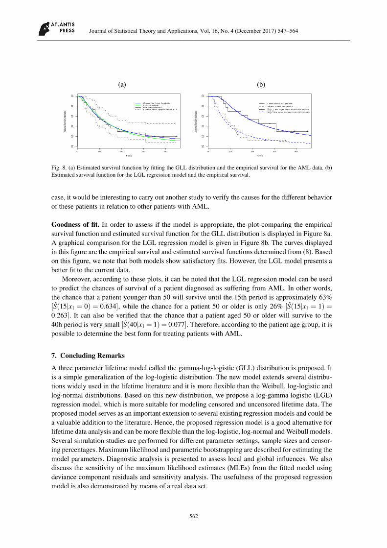
Fig. 8. (a) Estimated survival function by fitting the GLL distribution and the empirical survival for the AML data. (b)Estimated survival function for the LGL regression model and the empirical survival.

case, it would be interesting to carry out another study to verify the causes for the different behaviorof these patients in relation to other patients with AML.

Goodness of fit. In order to assess if the model is appropriate, the plot comparing the empiricalsurvival function and estimated survival function for the GLL distribution is displayed in Figure 8a.A graphical comparison for the LGL regression model is given in Figure 8b. The curves displayedin this figure are the empirical survival and estimated survival functions determined from (8). Basedon this figure, we note that both models show satisfactory fits. However, the LGL model presents abetter fit to the current data.

Moreover, according to these plots, it can be noted that the LGL regression model can be usedto predict the chances of survival of a patient diagnosed as suffering from AML. In other words,the chance that a patient younger than 50 will survive until the 15th period is approximately 63%[S(15|x1 = 0) = 0.634], while the chance for a patient 50 or older is only 26% [S(15|x1 = 1) =0.263]. It can also be verified that the chance that a patient aged 50 or older will survive to the40h period is very small [S(40|x1 = 1) = 0.077]. Therefore, according to the patient age group, it ispossible to determine the best form for treating patients with AML.

7. Concluding Remarks

A three parameter lifetime model called the gamma-log-logistic (GLL) distribution is proposed. Itis a simple generalization of the log-logistic distribution. The new model extends several distribu-tions widely used in the lifetime literature and it is more flexible than the Weibull, log-logistic andlog-normal distributions. Based on this new distribution, we propose a log-gamma logistic (LGL)regression model, which is more suitable for modeling censored and uncensored lifetime data. Theproposed model serves as an important extension to several existing regression models and could bea valuable addition to the literature. Hence, the proposed regression model is a good alternative forlifetime data analysis and can be more flexible than the log-logistic, log-normal and Weibull models.Several simulation studies are performed for different parameter settings, sample sizes and censor-ing percentages. Maximum likelihood and parametric bootstrapping are described for estimating themodel parameters. Diagnostic analysis is presented to assess local and global influences. We alsodiscuss the sensitivity of the maximum likelihood estimates (MLEs) from the fitted model usingdeviance component residuals and sensitivity analysis. The usefulness of the proposed regressionmodel is also demonstrated by means of a real data set.


562

Acknowledgments

This work was supported by FAPESP grant 2010/04496-2, Brazil.

Appendix

Theorem A.1. Let (Ω,F ,P) be a given probability space and let H = [a,b] be an interval for somea < b (a =−∞ , b = ∞might as well be allowed) . Let Y : Ω → H be a continuous random variablewith the distribution function F and let h and g be two real functions defined on H such that

E [g(Y ) | Y ≥ y]E [h(Y ) | Y ≥ y]

= η (y) , y ∈ H

is defined with some real function η . Assume that h,g ∈C1 (H), η ∈C2 (H) and F is twice contin-uously differentiable and strictly monotone function on the set H. Finally, assume that the equationηh = g has no real solution in the interior of H. Then F is uniquely determined by the functions h,gand η , particularly

F (y) =∫ y

aC∣∣∣∣ η ′ (u)η (u)h(u)−g(u)

∣∣∣∣exp(−s(u)) du ,

where the function s is a solution of the differential equation s′ = η ′hηh − g and C is a constant, chosen

to make∫

H dF = 1.

References[1] C. Alexander, G.M. Cordeiro, E.M.M. Ortega and J.M. Sarabia, Generalized beta-generated distribu-

tion, Computational Statistics and Data Analysis 56 (2012) 1880–1897.[2] A.C. Atkinson, Plots, transformations and regression: an introduction to graphical methods of diag-

nostic regression analysis, (University Press, Oxford, 1985).[3] M.V. Aarset, How to identify bathtub hazard rate, IEEE Transactions on Reliability 36 (1987) 106–108.[4] D. Collett, Modelling survival data in medical research, (Chapman & Hall, Boca Raton, London, New

York, 2003).[5] E.A. Colosimo and S.R. Giolo, Anlise de sobrevivłncia aplicada, (Edgard Blcher, So Paulo, 2006).[6] R.D. Cook, Assessment of local influence (with discussion), Journal of the Royal Statistical Society B

48 (1986) 133–169.[7] R.D. Cook and S. Weisberg, Residuals and influence in regression, (Chapman & Hall, Boca Raton,

London, New York, 1982).[8] G.M. Cordeiro and M. de Castro, A new family of generalized distributions, Journal of Statistical

Computation and Simulation 81 (2011) 883–898.[9] J.A. Doornik, An Object-Oriented Matrix Language Ox 5, (Timberlake Consultants Press, London,

2007).[10] B. Efron, Bootstrap methods: another look at the jackknife, The Annals of Statistics 7 (1979) 1–26.[11] B. Efron and R. Tibshirani, An introduction to the bootstrap, (Chapman & Hall, Boca Raton, London,

New York, 1993).[12] N. Eugene, C. Lee and F. Famoye, Beta-normal distribution and its applications, Communications in

Statistics - Theory and Methods 31 (2002) 497–512.[13] E.M. Hashimoto, G.M. Cordeiro and E.M.M. Ortega, The new Neyman type A beta Weibull model

with long-term survivors, Computational Statistics 28 (2013) 933–954.[14] J.F. Lawless, Statistical models and methods for lifetime data. (John Wiley & Sons, New York, 2003).[15] E.T. Lee and J.W. Wang, Statistical methods for survival data analysis, 3rd Edition, (John Wiley &

Sons, New Jersey, 2003).


563

[16] M.W.A. Ramos, G.M. Cordeiro, P.R.D. Marinho, C.R.B. Dias and G.G. Hamedani, The Zografos-Balakrishnan log-logistic distribution: properties and applications, Journal of Statistical Theory andApplications 12 (2013) 225–244.

[17] M.M. Ristic and N. Balakrishnan, The Gamma Exponentiated Exponential Distribution, Journal ofStatistical Computation and Simulation 82 (2012) 1191–1206.

[18] S.M. Ross, Simulation, (Elsevier Academic Press, Boston, 2006).[19] T.V.F. Santana, E.M.M. Ortega, G.M. Cordeiro and G.O. Silva, The Kumaraswamy-log-logistic distri-

bution, Journal of Statistical Theory and Applications 11 (2012) 265–291.[20] Z. Shayan, S.M.T. Ayatollahi and N. Zare, A parametric method for cumulative incidence modeling

with a new four-parameter log-logistic distribution, Theoretical Biology and Medical Modeling 8 (2011)1–11.

[21] M.M. Shoukri, I.U.M. Mian and D.S. Tracy, Sampling properties of estimators of the log-logistic dis-tribution with application to Canadian precipitation data, The Canadian Journal of Statistics 16 (1988)223–236.

[22] G.O. Silva, E.M.M. Ortega and G.A. Paula, Residuals for log-Burr XII regression models in survivalanalysis, Journal of Applied Statistics 38 (2011) 1435–1445.

[23] S. Weisberg, Applied linear regression, (John Wiley & Sons, New York, 2005).[24] F.C. Xie and B.C. Wei, Diagnostics analysis in censored generalized Poisson regression model, Journal

of Statistical Computation and Simulation 77 (2007) 695–708.[25] N. Zare, M. Doostfatemeh and A. Rezaianzadeh, Modeling of breast cancer prognostic factors using a

parametric log-logistic model in Fars Province, Southern Iran, Asian Pacific Journal of Cancer Preven-tion 13 (2012) 533–1537.

[26] K. Zografos and N. Balakrishnan, On families of beta-and generalized gama-generated distributionsand associated inference, Statistical Methodology 6 (2009) 344–362.


564

the log-gamma-logistic regression model: estimation

Documents