the long-range economic assumptions for the … · the long-range economic assumptions . for the...
TRANSCRIPT
THE LONG-RANGE ECONOMIC ASSUMPTIONS FOR THE 2018 TRUSTEES REPORT
OFFICE OF THE CHIEF ACTUARY SOCIAL SECURITY ADMINISTRATION
June 5, 2018

Page 2
PRINCIPAL ECONOMIC ASSUMPTIONS OVERVIEW Sections 1 PRODUCTIVITY 2 PRICE INFLATION 3 AVERAGE REAL WAGE DIFFERENTIAL 4 UNEMPLOYMENT RATE 5 ANNUAL TRUST FUND REAL INTEREST RATE 6 RATIO OF OASDI TAXABLE PAYROLL TO COVERED EARNINGS
Overview, Page 1
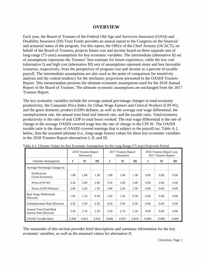
OVERVIEW Each year, the Board of Trustees of the Federal Old-Age and Survivors Insurance (OASI) and Disability Insurance (DI) Trust Funds provides an annual report to the Congress on the financial and actuarial status of the program. For this report, the Office of the Chief Actuary (OCACT), on behalf of the Board of Trustees, projects future cost and income based on three separate sets of long-range (75-year) assumptions for key economic variables. The intermediate (alternative II) set of assumptions represents the Trustees’ best estimate for future experience, while the low cost (alternative I) and high cost (alternative III) sets of assumptions represent more and less favorable scenarios, respectively, from the perspective of program cost and income as a percent of taxable payroll. The intermediate assumptions are also used as the point of comparison for sensitivity analysis and the central tendency for the stochastic projections presented in the OASDI Trustees Report. This memorandum presents the ultimate economic assumptions used for the 2018 Annual Report of the Board of Trustees. The ultimate economic assumptions are unchanged from the 2017 Trustees Report. The key economic variables include the average annual percentage changes in total-economy productivity, the Consumer Price Index for Urban Wage Earners and Clerical Workers (CPI-W), and the gross domestic product (GDP) deflator, as well as the average real wage differential, the unemployment rate, the annual trust fund real interest rate, and the taxable ratio. Total-economy productivity is the ratio of real GDP to total hours worked. The real wage differential is the rate of change in the average OASDI covered wage less the rate of change in the CPI-W. The OASDI taxable ratio is the share of OASDI covered earnings that is subject to the payroll tax. Table A.1, below, lists the assumed ultimate (i.e., long-range future) values for these key economic variables in the 2018 Trustees Report alternatives I, II, and III. Table A.1: Ultimate Values for Key Economic Assumptions for the Long-Range (75-year) Projection Period
2018 Trustees Report Alternative
2017 Trustees Report Alternative
2018 Trustees Report Less 2017 Trustees Report
Ultimate Assumptions I II III I II III I II III
Average Percentage Change In:
Productivity (Total-Economy) 1.98 1.68 1.38 1.98 1.68 1.38 0.00 0.00 0.00
Prices (CPI-W) 3.20 2.60 2.00 3.20 2.60 2.00 0.00 0.00 0.00
Prices (GDP Deflator) 2.90 2.20 1.50 2.90 2.20 1.50 0.00 0.00 0.00
Real Wage Differential (Percent) 1.82 1.20 0.58 1.82 1.20 0.58 0.00 0.00 0.00
Unemployment Rate (Percent) 4.50 5.50 6.50 4.50 5.50 6.50 0.00 0.00 0.00
Annual Trust Fund Real Interest Rate (Percent) 3.20 2.70 2.20 3.20 2.70 2.20 0.00 0.00 0.00
OASDI Taxable Ratio 0.840 0.825 0.810 0.840 0.825 0.810 0.000 0.000 0.000
The remainder of this section provides brief descriptions and summary information for the key economic variables, as well as the assumed values for alternative II.
Overview, Page 2
Productivity − The rate of growth in total-economy productivity is the fundamental component contributing to the real growth rate of average earnings. OCACT uses a weighted average of the productivity growth rates in economic sectors, where the weights are the shares of each sector in total GDP. The economic sectors include the nonfarm business sector, the farm sector, the household sector, the nonprofit institutions sector, and the general government sector. In the long-range period, OCACT assumes that the sector weights are approximately fixed. Based on an analysis of the data and future trends, the ultimate assumed growth rates for the sectors are as follows: 2.06 percent for the non-farm business sector, 2.06 percent for the farm sector, 1.68 for the household sector, 0.0 percent for the nonprofit sector, and 0.0 for the government sector. The weighted average of the assumed sector productivity growth rates is equal to the Trustees’ assumed ultimate long-range average annual rate of growth in total-economy productivity of 1.68 percent. Price Inflation − The rate of growth in the CPI-W is used to determine the cost of living adjustment (COLA). The average annual growth rate in the CPI-W was about 2.6 percent over the last two complete economic cycles from 1989 to 2007. OCACT expects that monetary policy will continue to target relatively low inflation, but will not be able to prevent occasional bursts of inflation caused by demand and supply shocks. Accordingly, the ultimate long-range average annual percentage change in the CPI-W is assumed to be 2.6 percent. The GDP deflator is another measure of price inflation. It is used in projecting the level of aggregate GDP and wages and, therefore, OASDI tax revenues. The CPI-W and the GDP deflator are assumed to grow at different rates in the future due to two inherent differences in their computational methods and coverage. One difference is the way that groups of goods and services are weighted in computing the overall price increases. Unlike the CPI-W, the GDP deflator formula accounts for shifts in the distribution of purchases across broad groups of goods and services (“upper level substitution”), and thus reflects changes in the behavior of consumers in response to changes in relative price of items that are not close substitutes. Because of this difference, the GDP deflator measures lower price inflation compared to the CPI-W. The Bureau of Labor Statistics (BLS) provides data showing that the behavioral response of consumers to relative price changes would have lowered the average annual rate of change in the CPI-U (and therefore CPI-W) between 1990 and 2015 by about 0.3 percentage point. OCACT expects the future average annual rate of change in the GDP deflator to be 0.3 percentage point below the average annual rate of change in the CPI-W due to this difference in computational methods. The second important difference between the CPI-W and the GDP deflator is coverage. The CPI-W measures the annual growth rate in prices covered by consumer expenditures, while the GDP deflator reflects the annual growth rate in prices covered by all consumption, investment, and government expenditures. OCACT expects that the net effect of difference in coverage is that the average annual growth rate in the GDP deflator will be about 0.1 percentage point lower than the average annual growth rate in the CPI-W. Thus, the ultimate assumed long-range average annual growth rate in the GDP deflator is 2.2 percent, or 0.4 percentage point below the 2.6 percent assumed ultimate long-range average annual
Overview, Page 3
growth rate in the CPI-W. The price differential of 0.4 percentage point is the sum of 0.3 percentage point for computational difference and 0.1 percentage point for coverage difference. Average Real Wage Differential – Annual real wage differentials vary to a small degree over the last 65 years of the 75-year projection horizon (i.e., 2027 to 2092), averaging 1.20 percent, unchanged from the 2017 report. The Centers for Medicare and Medicaid Services (CMS) projects approximately the same average growth in the share of employee compensation that is provided as employer-sponsored group health insurance (ESI) as in last year’s report. OCACT expects the ultimate average annual rate of change in the average OASDI covered wage to be approximately the same as for (1) average U.S. wages and (2) average U.S. earnings (which include the self-employed). The average annual real growth rate in average U.S. earnings is assumed to be 1.17 percent over the 65-year period. This reflects average annual changes of 1.68 percent for total-economy productivity, -0.4 percent for the price differential, -0.06 percent for the average earnings ratio, 0.0 percent for the compensation ratio, and -0.05 percent for the average hours worked per week. Unemployment Rate – The aggregate civilian unemployment rate, adjusted for the 2011 age-sex distribution of the labor force, averaged about 5.2 percent over the last five complete economic cycles from 1966 to 2007, and about 5.6 percent over the last 50 years (from 1966 to 2016). In the future, the projected decline in the overall growth rate in the labor force will likely put some downward pressure on the aggregate unemployment rate. The ultimate long-range civilian age-sex adjusted unemployment rate is assumed to be 5.5 percent. Annual Trust Fund Real Interest Rate – The real interest rate (real effective annual yield) on the special public debt obligations issuable to the trust funds for a given year is defined as the nominal effective annual yield adjusted for the increase in the CPI-W for the first year after issue. Future real interest rates on long-term Treasury securities will depend in part on the market view of the stability and solidity of the domestic financial markets and the domestic economy. Real ex-post (actual) interest rates on long-term Treasury securities averaged 3.17 percent over the last five economic cycles (from 1966 to 2007). Real interest rates have been substantially lower recently due to the weak economy in most of the developed world. The assumed ultimate long-range real interest rate for new issues is 2.7 percent. This ultimate assumption is consistent with a sustainable domestic fiscal policy over the long-range period and a gradual return to the sustainable rate of economic growth throughout the developed world. OASDI Taxable Ratio – The OASDI taxable ratio is the share of OASDI covered earnings that is subject to the payroll tax. It is a fundamental component to projections of taxable payroll. This ratio declined substantially between 1983 and 2001, and has continued to decline between 2001 and 2014, but much more slowly. The ratio is expected to decline even more slowly over the next 12 years, and to stabilize thereafter. The assumed ultimate long-range taxable ratio is 82.5 percent.
Productivity, Page 1
1. PRODUCTIVITY
THE 2018 TRUSTEES REPORT OFFICE OF THE CHIEF ACTUARY, SOCIAL SECURITY ADMINISTRATION
TABLE OF CONTENTS PAGE 1 PRODUCTIVITY................................................................................................................... 2
1.1 SUMMARY ...................................................................................................................................................... 2 1.2 RECENT BEA AND BLS DATA REVISIONS ...................................................................................................... 2 1.3 PRODUCTIVITY GROWTH RATES FOR MAJOR SECTORS AND OVER LONG TIME PERIODS AND ECONOMIC CYCLES ...................................................................................................................................................................... 3
1.3.1 Sector Productivity Growth Rates ......................................................................................................... 5 1.3.1.1 Nonfarm Business (NFB) ................................................................................................................................... 5 1.3.1.2 Farm ................................................................................................................................................................... 6 1.3.1.3 Nonprofit Institutions (NI) ................................................................................................................................. 6 1.3.1.4 General Government (GOV) .............................................................................................................................. 7 1.3.1.5 Households ......................................................................................................................................................... 8
1.3.2 Total-Economy Productivity Growth Rate ........................................................................................... 10 1.4 PROJECTIONS FROM OTHER SOURCES ........................................................................................................... 10 1.5 APPENDIX ..................................................................................................................................................... 16
TABLE OF TABLES PAGE TABLE 1.1: ASSUMED ULTIMATE ANNUAL RATES OF INCREASE IN TOTAL-ECONOMY PRODUCTIVITY ......................... 2 TABLE 1.2: HISTORICAL AVERAGE ANNUAL RATES OF INCREASE IN TOTAL-ECONOMY PRODUCTIVITY AND ITS
COMPONENTS (%) .................................................................................................................................................. 3 TABLE 1.3: ULTIMATE AVERAGE ANNUAL RATES OF INCREASE IN TOTAL-ECONOMY PRODUCTIVITY AND ITS
COMPONENTS FOR THE 2018 TRUSTEES REPORT .................................................................................................... 3 TABLE 1.4: TOTAL-ECONOMY PRODUCTIVITY: COMPOUND ANNUAL RATES OF GROWTH (%) BASE YEAR = 2009 .... 12 TABLE 1.5: NONFARM BUSINESS PRODUCTIVITY: COMPOUND ANNUAL RATES OF GROWTH (%) BASE YEAR = 2009 14
Productivity, Page 2
1 Productivity
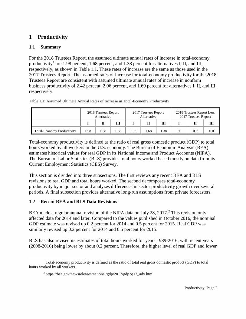
1.1 Summary For the 2018 Trustees Report, the assumed ultimate annual rates of increase in total-economy productivity1 are 1.98 percent, 1.68 percent, and 1.38 percent for alternatives I, II, and III, respectively, as shown in Table 1.1. These rates of increase are the same as those used in the 2017 Trustees Report. The assumed rates of increase for total-economy productivity for the 2018 Trustees Report are consistent with assumed ultimate annual rates of increase in nonfarm business productivity of 2.42 percent, 2.06 percent, and 1.69 percent for alternatives I, II, and III, respectively. Table 1.1: Assumed Ultimate Annual Rates of Increase in Total-Economy Productivity
2018 Trustees Report Alternative
2017 Trustees Report Alternative
2018 Trustees Report Less 2017 Trustees Report
I II III I II III I II III
Total-Economy Productivity 1.98 1.68 1.38 1.98 1.68 1.38 0.0 0.0 0.0
Total-economy productivity is defined as the ratio of real gross domestic product (GDP) to total hours worked by all workers in the U.S. economy. The Bureau of Economic Analysis (BEA) estimates historical values for real GDP in its National Income and Product Accounts (NIPA). The Bureau of Labor Statistics (BLS) provides total hours worked based mostly on data from its Current Employment Statistics (CES) Survey. This section is divided into three subsections. The first reviews any recent BEA and BLS revisions to real GDP and total hours worked. The second decomposes total-economy productivity by major sector and analyzes differences in sector productivity growth over several periods. A final subsection provides alternative long-run assumptions from private forecasters.
1.2 Recent BEA and BLS Data Revisions BEA made a regular annual revision of the NIPA data on July 28, 2017.2 This revision only affected data for 2014 and later. Compared to the values published in October 2016, the nominal GDP estimate was revised up 0.2 percent for 2014 and 0.5 percent for 2015. Real GDP was similarly revised up 0.2 percent for 2014 and 0.5 percent for 2015. BLS has also revised its estimates of total hours worked for years 1989-2016, with recent years (2008-2016) being lower by about 0.2 percent. Therefore, the higher level of real GDP and lower
1 Total-economy productivity is defined as the ratio of total real gross domestic product (GDP) to total
hours worked by all workers. 2 https://bea.gov/newsreleases/national/gdp/2017/gdp2q17_adv.htm
Productivity, Page 3
level of total hours worked in the revised data implies a higher level of productivity for the period.3
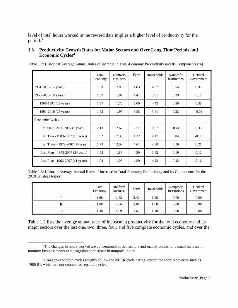
1.3 Productivity Growth Rates for Major Sectors and Over Long Time Periods and Economic Cycles4
Table 1.2: Historical Average Annual Rates of Increase in Total-Economy Productivity and Its Components (%)
Total Economy
Nonfarm Business
Farm Households Nonprofit Institutions
General Government
1951-2016 (65 years) 1.89 2.03 4.83 4.52 0.54 0.33
1966-2016 (50 years) 1.59 1.84 4.41
3.91
0.39 0.17
1966-1991 (25 years) 1.57
1.70
5.00 4.42
0.56 0.35
1991-2016 (25 years)
1.62 1.97 3.83 3.41
0.22 -0.01
Economic Cycles
Last One - 2000-2007 (7 years) 2.13
2.62 2.77 0.97 -0.44 0.33
Last Two - 1989-2007 (18 years) 1.92 2.33 4.32 4.17 0.04 -0.03
Last Three - 1979-2007 (28 years) 1.73
2.02 4.61 3.88 0.16 0.21
Last Four - 1973-2007 (34 years) 1.62 1.88 4.50 3.82 0.19 0.12
Last Five - 1966-2007 (41 years) 1.73
1.98 4.59 4.22 0.42 0.16
Table 1.3: Ultimate Average Annual Rates of Increase in Total-Economy Productivity and Its Components for the 2018 Trustees Report
Total Economy
Nonfarm Business Farm Households Nonprofit
Institutions General
Government
I 1.98 2.42 2.42 1.98 0.00 0.00
II 1.68 2.06 2.06 1.68 0.00 0.00
III 1.38 1.69 1.69 1.38 0.00 0.00
Table 1.2 lists the average annual rates of increase in productivity for the total economy and its major sectors over the last one, two, three, four, and five complete economic cycles, and over the
3 The changes in hours worked are concentrated in two sectors and mainly consist of a small increase in
nonfarm business hours and a significant decrease in nonprofit hours.
4 Peaks in economic cycles roughly follow the NBER cycle dating, except for short recoveries such as 1980-81, which are not counted as separate cycles.
Productivity, Page 4
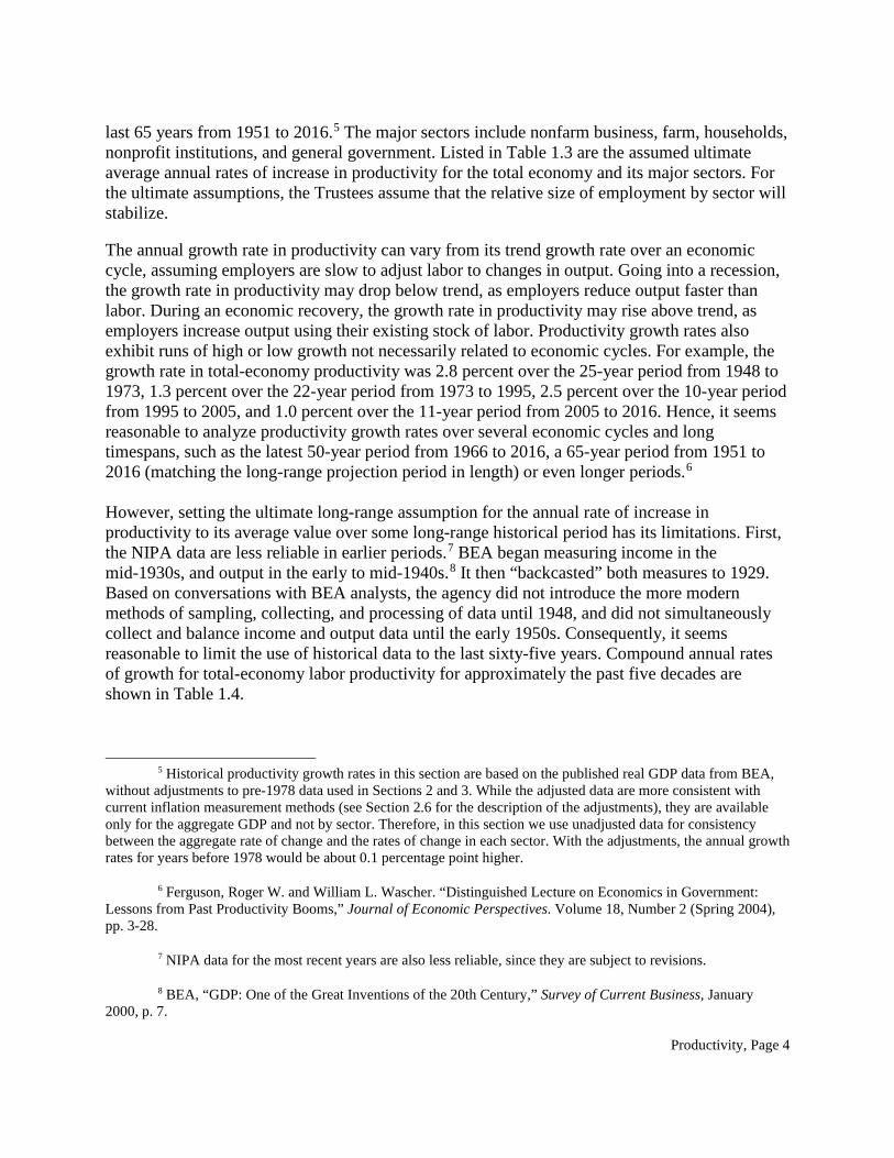
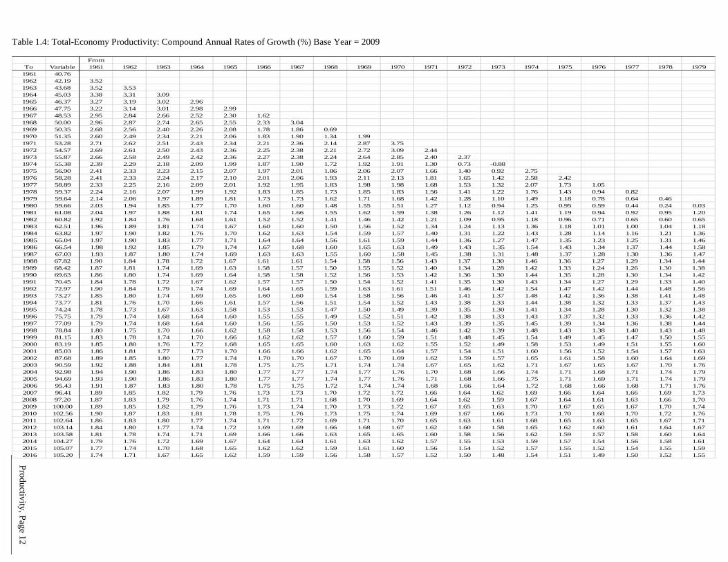
last 65 years from 1951 to 2016.5 The major sectors include nonfarm business, farm, households, nonprofit institutions, and general government. Listed in Table 1.3 are the assumed ultimate average annual rates of increase in productivity for the total economy and its major sectors. For the ultimate assumptions, the Trustees assume that the relative size of employment by sector will stabilize. The annual growth rate in productivity can vary from its trend growth rate over an economic cycle, assuming employers are slow to adjust labor to changes in output. Going into a recession, the growth rate in productivity may drop below trend, as employers reduce output faster than labor. During an economic recovery, the growth rate in productivity may rise above trend, as employers increase output using their existing stock of labor. Productivity growth rates also exhibit runs of high or low growth not necessarily related to economic cycles. For example, the growth rate in total-economy productivity was 2.8 percent over the 25-year period from 1948 to 1973, 1.3 percent over the 22-year period from 1973 to 1995, 2.5 percent over the 10-year period from 1995 to 2005, and 1.0 percent over the 11-year period from 2005 to 2016. Hence, it seems reasonable to analyze productivity growth rates over several economic cycles and long timespans, such as the latest 50-year period from 1966 to 2016, a 65-year period from 1951 to 2016 (matching the long-range projection period in length) or even longer periods.6 However, setting the ultimate long-range assumption for the annual rate of increase in productivity to its average value over some long-range historical period has its limitations. First, the NIPA data are less reliable in earlier periods.7 BEA began measuring income in the mid-1930s, and output in the early to mid-1940s.8 It then “backcasted” both measures to 1929. Based on conversations with BEA analysts, the agency did not introduce the more modern methods of sampling, collecting, and processing of data until 1948, and did not simultaneously collect and balance income and output data until the early 1950s. Consequently, it seems reasonable to limit the use of historical data to the last sixty-five years. Compound annual rates of growth for total-economy labor productivity for approximately the past five decades are shown in Table 1.4.
5 Historical productivity growth rates in this section are based on the published real GDP data from BEA,
without adjustments to pre-1978 data used in Sections 2 and 3. While the adjusted data are more consistent with current inflation measurement methods (see Section 2.6 for the description of the adjustments), they are available only for the aggregate GDP and not by sector. Therefore, in this section we use unadjusted data for consistency between the aggregate rate of change and the rates of change in each sector. With the adjustments, the annual growth rates for years before 1978 would be about 0.1 percentage point higher.
6 Ferguson, Roger W. and William L. Wascher. “Distinguished Lecture on Economics in Government: Lessons from Past Productivity Booms,” Journal of Economic Perspectives. Volume 18, Number 2 (Spring 2004), pp. 3-28.
7 NIPA data for the most recent years are also less reliable, since they are subject to revisions.
8 BEA, “GDP: One of the Great Inventions of the 20th Century,” Survey of Current Business, January 2000, p. 7.
Productivity, Page 5
A second important limitation is that a significant portion of the total historical average annual rate of increase in total-economy productivity occurred because of shifts in workers from relatively low- to high-productivity jobs. For example, over the 50-year period from 1966 to 2016, the ratio of agricultural to total-economy hours worked declined from about 0.050 to 0.017, and the ratio of agricultural to total nominal GDP declined from about 0.026 to 0.007. Furthermore, although farm productivity grew faster than that of any other sector over the last 50 years, the average level of productivity for agricultural workers in 2016 was about 47 percent of the average level of productivity for all workers. This shift complicates the consideration of historical experience. The assumed ultimate long-range value for the annual rate of increase in total-economy productivity should be consistent with the average value over a long-range historical period with adjustment for differences between conditions of the past and conditions expected for the future. The average long-range historical value is inflated due to sectoral shifts in employment that are not expected to continue into the future.9 This problem can be resolved by removing the effects of sectoral shifts in employment from the historical record or, more simply, by setting the ultimate long-range value for the annual rate of increase in total-economy productivity to a weighted average of the expected ultimate long-range values for the annual rate of increase in productivity for each sector.
1.3.1 Sector Productivity Growth Rates
1.3.1.1 Nonfarm Business (NFB) The average annual growth rate in NFB productivity was 2.62 percent over the last economic cycle (i.e., a 7-year period from 2000 to 2007), and 2.33 percent over the last two economic cycles (18-year period from 1989 to 2007). These relatively high growth rates reflect the heavy influence of the 1995-2005 “new economy” period characterized by rapid improvements in computers and their assimilation into the economy. Looking at longer periods, the average annual growth rate in NFB productivity was 2.02 percent over the last three economic cycles (28-year period from 1979 to 2007), 1.88 percent over the last four economic cycles (34-year period from 1973 to 2007), and 1.98 percent over the last five economic cycles (41-year period from 1966 to 2007). These productivity growth rates include the effects of a relatively low growth rate period from 1973 to 1995. This slowdown has been attributed to a shift in employment from relatively high-productivity manufacturing jobs to low-productivity service jobs, and to the influx of new unskilled baby-boomers into the workforce. Historical compound annual rates of growth in labor productivity for the nonfarm business sector are shown in Table 1.5.
9 For example, the 0.033 decline (i.e., from 0.050 to 0.017) in the ratio of agriculture to total-economy hours worked over the last fifty years can’t be repeated in the future since the level of the ratio in 2016 is only 0.017 and it cannot become negative.
Productivity, Page 6
On balance, the 1.98 percent average annual growth rate for NFB productivity over the last five economic cycles (1966 to 2007) may be somewhat below the most reasonable assumption for the ultimate growth rate. Although the faster productivity growth over the last two economic cycles has been followed by slow productivity growth since the last cycle (the growth rate in NFB productivity has averaged only 1.19 percent over the 9-year period from 2007 to 2016), both the recent complete economic cycles and the longest available period of good data point to a somewhat higher long-run rate of growth. (The growth rate in NFB productivity over the last 65 years was 2.03 percent and would be somewhat higher if pre-1978 inflation adjustments were consistent with today’s methodology.) Thus, the assumed ultimate rate of increase in NFB productivity is 2.06 percent. This rate of increase is unchanged from the 2017 Trustees Report.
1.3.1.2 Farm The average annual growth rate in farm productivity was about 4.41 percent from 1966 to 2016. A significant portion of the relatively high growth rate in farm productivity was due to a shift in farm operation and ownership from smaller farms run by the self-employed to larger, more efficient and capital-intensive farms run by corporations. For example, based on BLS’ Current Population Survey (CPS) data, the ratio of self-employed to all workers in the agricultural sector fell from about 0.63 in 1966 to 0.35 in 2016. For the long-range future, this shift is expected to slow and the difference in the productivity growth rates between the farm and nonfarm sectors is expected to decline to zero. Thus, the assumed ultimate rate of increase in farm productivity is 2.06 percent, or equal to the assumed ultimate average annual growth rate in NFB productivity.
1.3.1.3 Nonprofit Institutions (NI) The average annual rate of change in NI productivity was 0.56 percent over the 25-year period from 1966 to 1991, 0.22 percent over the 25-year period from 1991 to 2016, and 0.39 percent over the combined 50-year period from 1966 to 2016. The pattern of growth rates in NI productivity, with periods of positive and negative values, is largely due to shifts in employment within the NI sector. In the NIPA, NI labor compensation accounts for about 84 percent of NI nominal GDP. NI compensation is summed from five subsectors including education, health, social, religious, and business services. For each subsector, the level of real output is defined as the product of the level of average compensation per hour in a base year (currently 2009) and the level of hours worked. This means that the level of productivity in each subsector is a constant (i.e., the average compensation per hour in a base year), and that the growth rate in productivity in each sector is zero. However, this also means that the level of productivity for the total NI sector is a weighted average of the levels of productivity in the subsectors, and that the growth rate in total NI productivity may be positive (or negative), due to shifts in employment from sectors with relatively low (high) average compensation to sectors with relatively high (low) compensation. In fact, BEA data indicate that the average annual compensation in health services has been higher than the average annual compensation in other service sectors since the mid-1970s, and that the growth in employment in health services over the 25-year period from 1966 to 1991 was
Productivity, Page 7
higher than the growth in employment in other service sectors. The NIPA include data on compensation and full-time equivalent employment in health care, educational services, and social assistance.10 These three sectors are mostly composed of NI workers.11 The data show that the level of average annual compensation for full-time equivalent employment in 2016 was $72,900, $58,300, and $33,400 in health care, educational services, and social assistance, respectively. The data also show that the ratio of full-time equivalent employment in the health sector to the total for all three sectors rose from about 0.45 in 1966 to 0.61 in 1986, declined to 0.57 in 2000, and remained relatively stable thereafter.12 Thus, the data indicate that the relative increase in employment in health services significantly contributed to the average annual rate of increase in NI productivity of 0.56 percent over the 25-year period from 1966 to 1991. The data also indicate that the subsequent relative stability in the growth rates in employment across NI subsectors significantly contributed to the decline in the NI productivity growth rate to 0.22 percent over the 25-year period from 1991 to 2016. In the future, it seems reasonable to assume that the more recent historical trend in employment will continue, and that the ultimate long-range growth rates in employment in the NI subsectors will be roughly equal.13 Thus, the assumed ultimate long-range growth rate in NI productivity is zero.
1.3.1.4 General Government (GOV) The average annual rate of increase in GOV productivity was 0.35 percent over the 25-year period from 1966 to 1991 and -0.01 percent over the 25-year period from 1991 to 2016. These relatively small growth rates in GOV productivity are due to shifts in employment within the GOV sector. GOV labor compensation accounts for about 79 percent of GOV nominal GDP.14 GOV compensation is summed from three primary subsectors: federal civilian, federal military, and state and local government. As with the NI subsector, the level of productivity in each subsector is a constant (i.e., the average compensation per hour in a base year), and the growth rate in productivity in each sector is zero. However, this also means that the level of productivity for the
10 BEA, NIPA, Tables 6.2B through 6.2D and Tables 6.5B through 6.5D http://www.bea.gov/iTable/iTable.cfm?ReqID=9&step=1.
11 BEA, “Income and Outlays of Households and of Nonprofit Institutions Serving Households,” Survey of Current Business, April 2003, p. 14 http://www.bea.gov/scb/pdf/2003/04april/0403household.pdf.
12 NIPA categories of services changed in 1998, so present ratios are not directly comparable with the old ones. The ratio declined from 0.61 in 1982-1987 to 0.57 in 2000 (the data for 1998-2000 are available both under the old and the new categorization), and remained roughly constant at 0.71 under the new categorization from 2000 to 2011. However, it has since declined to 0.69 for 2013 through 2016.
13Given that the overall assumptions reflect a continued growth in the health sector as a percent of GDP, this faster growth is assumed to occur in the for-profit sector of the economy.
14 BEA, NIPA, Table 3.10.5
Productivity, Page 8
total GOV sector is a weighted average of the levels of productivity in the subsectors, and that the growth rate in total GOV productivity may be positive (negative), due to shifts in employment from sectors with relatively low (high) average compensation to sectors with relatively high (low) compensation.15 The relatively small, positive growth rate in GOV productivity over some historical periods is due to shifts in employment between subsectors. In the future, the growth rate in GOV productivity could be negative, reflecting a reversal of historical trends. For the future, however, it seems reasonable to assume that the ultimate long-range growth rates in employment in the GOV subsectors will be about equal and that the assumed ultimate long-range growth rate in GOV productivity will be zero.16
1.3.1.5 Households In the NIPA, nominal GDP in the household sector is the sum of the nominal compensation of private household workers and the nominal imputed output of owner-occupied housing (IOH). In 2016, the nominal compensation of private household workers made up only about 1.5 percent of the total nominal GDP in the household sector. Though this component is relatively small, it is useful to analyze each component of GDP in the household sector. Compensation of Household Workers - As with NI and GOV compensation sectors, BEA sets the real growth rate in GDP equal to the growth rate in hours worked. Hence, the growth rate in productivity is, by definition, zero. Imputed Output of Owner-Occupied Housing (IOH) - Renters of apartments and homes pay rent and receive streams of housing services. BEA includes these business transactions in the NIPA. Though the owners of homes pay no rent and have no business transactions, they receive similar streams of housing services. Hence, for consistency, BEA estimates the real and nominal values of housing services received by those who own their own homes (i.e., real and nominal IOH) and includes these amounts in the NIPA. BEA’s inclusion of IOH in GDP creates a problem. Since IOH has no associated measure of labor hours worked, how should it be included when estimating historical and projecting future growth rates in sector and total-economy productivity? There are two approaches in handling IOH in projections of total-economy productivity for the long-range.
15 BEA, “Government Transactions, Methodology Papers: U.S. National Income and Product Accounts,” September 2005, http://www.bea.gov/national/pdf/mp5.pdf.
16 Beginning with the 2017 Report, OCACT estimates that the number of active military will remain constant rather than grow in proportion to civilian employment. This implies a gradual shift in the weights of civilian government and the military, and a resulting small decrease in average productivity of the government sector, but the effect is small.
Productivity, Page 9
First, total real GDP could be projected as the sum of projections for real IOH and real GDP less IOH. Real GDP less IOH would be the product of the total-economy-less-IOH productivity and total hours worked. The ultimate average annual growth rate in total-economy-less-IOH productivity could be set to the weighted average of the assumed ultimate average annual growth rates in sector productivity.17 Real IOH could be projected as a fixed ratio to total real GDP less IOH. 18 Total real GDP could then be constructed as the sum of real IOH and real GDP less IOH. As a second and equivalent approach, household productivity could be defined as the sum of real IOH and real output of private household workers to the total hours worked of private household workers (as in Table 1.2). Using this definition, the average annual rate of increase in productivity for private household workers over the 50-year period from 1966 to 2016 was about 3.91 percent. In the future, however, the average annual growth rate in productivity for private household workers is expected to be much lower. In fact, it is expected to equal the average annual growth rate of total-economy-less-IOH productivity, as described in the first approach.19 The ultimate average annual growth rate in total-economy productivity could be set to the weighted average of the assumed ultimate average annual growth rates in sector productivity.20 Finally, total real GDP would be the product of total-economy productivity and hours worked.
17 Sector weights would be defined as the ratio of sector to total nominal GDP less IOH. 18 Over the 30-year period from 1987 through 2016, the ratio of real IOH to real GDP less IOH has been
fairly constant and averaged 0.078. 19 If,
Pph = Real IOH / Hph Pxph = Real GDP less IOH / Hxph
Then,
. . . Pph = Real IOH – Hph
. . . Pxph = Real GDP less IOH – Hxph
Assuming, . .
Real IOH = Real GDP less IOH . .
Hph = Hxph Then,
. . Pph = Pxph
Where, Pph = Productivity, private household
Pxph = Productivity, total economy less private household Hph = Hours worked, private household Hxph = Hours worked, total economy less private household .
Y = Rate of change in Y 20 In this second approach, sector weights would be defined as the ratio of sector to total nominal GDP.
Productivity, Page 10
1.3.2 Total-Economy Productivity Growth Rate The assumed ultimate growth rate in total-economy productivity is equal to a weighted average of the growth rates in sector productivity and employment (see Section 1.5 Appendix). This relationship is simplified by assuming that the ultimate long-range growth rate in employment in all sectors of the economy will be about equal, and that the ultimate long-range growth rates in productivity for the nonprofit institution, and general government sectors will be zero. Given these assumptions, the ultimate long-range growth rate in total-economy productivity is equal to the weighted average of the ultimate long-range growth rates in productivity in the farm, nonfarm business, and household sectors of the economy. Sector weights are defined as the ratio of sector to total nominal GDP. This “nominal output” weight for the farm sector declined from about 0.026 in 1966 to 0.007 in 2016, and it averaged about 0.008 over the last business cycle from 2000 to 2007. The nominal output weight for the nonfarm business sector was much more stable. It averaged 0.750 over the 25-year period from 1967 through 1991, 0.747 over the 25-year period from 1992 through 2016, and 0.749 over the last business cycle. For the future, the ultimate long-range values for the nominal output weights are assumed to remain at 0.75 for the nonfarm business sector and 0.01 for the farm sector. The nominal weight for the household sector rose from about 0.054 in 1977–79 to the historically high value of 0.077 in 2009. As mentioned, the increase in the weight occurred because the GDP deflator for IOH grew faster than the GDP deflator for all other goods over the period. More recently, the weight has fallen to 0.070 in 2014 and 2015, and 0.071 in 2016. In the future, OCACT expects the GDP deflator for IOH will grow at about the same rate as the GDP deflator for all other goods and that therefore the nominal weight for the household sector should stabilize at 0.07, close to its recent historical average. Sector weights can also be defined as the ratio of sector to total nominal GDP excluding IOH. In this case, the ultimate long-range values for the nominal output weights will be 0.0108 (i.e., 0.01 / (1.0 − 0.07)) for the farm sector, and 0.8065 (i.e., 0.75 / (1.0 − 0.07)) for the nonfarm sector. This analysis indicates that the long-range future growth rate in productivity for the total economy excluding IOH will be about 1.68 percent (i.e., 2.06 * (0.8065 + 0.0108)). It also indicates that the long-range future growth rate in productivity for the total economy including IOH will be about 1.68 percent (i.e., 2.06 * (0.75 + 0.01) + 1.68 * 0.07). Thus, for the 2018 Trustees Report, the assumed annual rates of increase in total-economy productivity are 1.98 percent, 1.68 percent, and 1.38 percent for alternatives I, II, and III, respectively. These rates of increase are the same as those used in the 2017 Trustees Report.
1.4 Projections from Other Sources IHS Markit (formerly Global Insight, Inc.) provides projections through 2047 in its latest long-run trend forecast (see The 30-Year Focus, Third Quarter, August 2017). IHS Markit projects that the average annual rate of increase in productivity will be about 1.57 percent for the nonfarm business sector and 1.36 percent for the total economy. Moody’s Analytics’ September
Productivity, Page 11
2017 forecast extends to 2047. For the 20-year period from 2027 to 2047, Moody’s Analytics projects the average annual growth rate in productivity will be about 1.6 percent for the nonfarm business sector and 1.3 percent for the total economy. The Office of Management and Budget (OMB) Mid-Session Review of the Fiscal Year 2018 Budget includes projections through 2027. The OMB annual growth rate for the total-economy productivity was 2.35 percent for 2027. The Congressional Budget Office (CBO) March 2017 report, The 2017 Long-Term Budget Outlook, includes projections through 2047. CBO’s average annual growth rate for total-economy productivity was 1.6 percent over the entire 30-year period and 1.6 percent over the last 10 years, 2038 through 2047. The Social Security Advisory Board’s 2015 Technical Panel on Assumptions and Methods recommended no changes to the assumed ultimate annual rate of increase in total-economy productivity of 1.68 percent in the 2015 Trustees Report, alternative II.
Productivity, Page 12
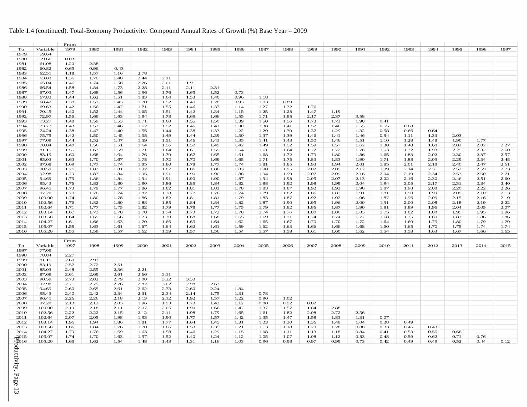
Table 1.4: Total-Economy Productivity: Compound Annual Rates of Growth (%) Base Year = 2009
FromTo Variable 1961 1962 1963 1964 1965 1966 1967 1968 1969 1970 1971 1972 1973 1974 1975 1976 1977 1978 1979
1961 40.761962 42.19 3.521963 43.68 3.52 3.531964 45.03 3.38 3.31 3.091965 46.37 3.27 3.19 3.02 2.961966 47.75 3.22 3.14 3.01 2.98 2.991967 48.53 2.95 2.84 2.66 2.52 2.30 1.621968 50.00 2.96 2.87 2.74 2.65 2.55 2.33 3.041969 50.35 2.68 2.56 2.40 2.26 2.08 1.78 1.86 0.691970 51.35 2.60 2.49 2.34 2.21 2.06 1.83 1.90 1.34 1.991971 53.28 2.71 2.62 2.51 2.43 2.34 2.21 2.36 2.14 2.87 3.751972 54.57 2.69 2.61 2.50 2.43 2.36 2.25 2.38 2.21 2.72 3.09 2.441973 55.87 2.66 2.58 2.49 2.42 2.36 2.27 2.38 2.24 2.64 2.85 2.40 2.371974 55.38 2.39 2.29 2.18 2.09 1.99 1.87 1.90 1.72 1.92 1.91 1.30 0.73 -0.881975 56.90 2.41 2.33 2.23 2.15 2.07 1.97 2.01 1.86 2.06 2.07 1.66 1.40 0.92 2.751976 58.28 2.41 2.33 2.24 2.17 2.10 2.01 2.06 1.93 2.11 2.13 1.81 1.65 1.42 2.58 2.421977 58.89 2.33 2.25 2.16 2.09 2.01 1.92 1.95 1.83 1.98 1.98 1.68 1.53 1.32 2.07 1.73 1.051978 59.37 2.24 2.16 2.07 1.99 1.92 1.83 1.85 1.73 1.85 1.83 1.56 1.41 1.22 1.76 1.43 0.94 0.821979 59.64 2.14 2.06 1.97 1.89 1.81 1.73 1.73 1.62 1.71 1.68 1.42 1.28 1.10 1.49 1.18 0.78 0.64 0.461980 59.66 2.03 1.94 1.85 1.77 1.70 1.60 1.60 1.48 1.55 1.51 1.27 1.12 0.94 1.25 0.95 0.59 0.44 0.24 0.031981 61.08 2.04 1.97 1.88 1.81 1.74 1.65 1.66 1.55 1.62 1.59 1.38 1.26 1.12 1.41 1.19 0.94 0.92 0.95 1.201982 60.82 1.92 1.84 1.76 1.68 1.61 1.52 1.52 1.41 1.46 1.42 1.21 1.09 0.95 1.18 0.96 0.71 0.65 0.60 0.651983 62.51 1.96 1.89 1.81 1.74 1.67 1.60 1.60 1.50 1.56 1.52 1.34 1.24 1.13 1.36 1.18 1.01 1.00 1.04 1.181984 63.82 1.97 1.90 1.82 1.76 1.70 1.62 1.63 1.54 1.59 1.57 1.40 1.31 1.22 1.43 1.28 1.14 1.16 1.21 1.361985 65.04 1.97 1.90 1.83 1.77 1.71 1.64 1.64 1.56 1.61 1.59 1.44 1.36 1.27 1.47 1.35 1.23 1.25 1.31 1.461986 66.54 1.98 1.92 1.85 1.79 1.74 1.67 1.68 1.60 1.65 1.63 1.49 1.43 1.35 1.54 1.43 1.34 1.37 1.44 1.581987 67.03 1.93 1.87 1.80 1.74 1.69 1.63 1.63 1.55 1.60 1.58 1.45 1.38 1.31 1.48 1.37 1.28 1.30 1.36 1.471988 67.82 1.90 1.84 1.78 1.72 1.67 1.61 1.61 1.54 1.58 1.56 1.43 1.37 1.30 1.46 1.36 1.27 1.29 1.34 1.441989 68.42 1.87 1.81 1.74 1.69 1.63 1.58 1.57 1.50 1.55 1.52 1.40 1.34 1.28 1.42 1.33 1.24 1.26 1.30 1.381990 69.63 1.86 1.80 1.74 1.69 1.64 1.58 1.58 1.52 1.56 1.53 1.42 1.36 1.30 1.44 1.35 1.28 1.30 1.34 1.421991 70.45 1.84 1.78 1.72 1.67 1.62 1.57 1.57 1.50 1.54 1.52 1.41 1.35 1.30 1.43 1.34 1.27 1.29 1.33 1.401992 72.97 1.90 1.84 1.79 1.74 1.69 1.64 1.65 1.59 1.63 1.61 1.51 1.46 1.42 1.54 1.47 1.42 1.44 1.48 1.561993 73.27 1.85 1.80 1.74 1.69 1.65 1.60 1.60 1.54 1.58 1.56 1.46 1.41 1.37 1.48 1.42 1.36 1.38 1.41 1.481994 73.77 1.81 1.76 1.70 1.66 1.61 1.57 1.56 1.51 1.54 1.52 1.43 1.38 1.33 1.44 1.38 1.32 1.33 1.37 1.431995 74.24 1.78 1.73 1.67 1.63 1.58 1.53 1.53 1.47 1.50 1.49 1.39 1.35 1.30 1.41 1.34 1.28 1.30 1.32 1.381996 75.75 1.79 1.74 1.68 1.64 1.60 1.55 1.55 1.49 1.52 1.51 1.42 1.38 1.33 1.43 1.37 1.32 1.33 1.36 1.421997 77.09 1.79 1.74 1.68 1.64 1.60 1.56 1.55 1.50 1.53 1.52 1.43 1.39 1.35 1.45 1.39 1.34 1.36 1.38 1.441998 78.84 1.80 1.75 1.70 1.66 1.62 1.58 1.58 1.53 1.56 1.54 1.46 1.42 1.39 1.48 1.43 1.38 1.40 1.43 1.481999 81.15 1.83 1.78 1.74 1.70 1.66 1.62 1.62 1.57 1.60 1.59 1.51 1.48 1.45 1.54 1.49 1.45 1.47 1.50 1.552000 83.19 1.85 1.80 1.76 1.72 1.68 1.65 1.65 1.60 1.63 1.62 1.55 1.52 1.49 1.58 1.53 1.49 1.51 1.55 1.602001 85.03 1.86 1.81 1.77 1.73 1.70 1.66 1.66 1.62 1.65 1.64 1.57 1.54 1.51 1.60 1.56 1.52 1.54 1.57 1.632002 87.68 1.89 1.85 1.80 1.77 1.74 1.70 1.70 1.67 1.70 1.69 1.62 1.59 1.57 1.65 1.61 1.58 1.60 1.64 1.692003 90.59 1.92 1.88 1.84 1.81 1.78 1.75 1.75 1.71 1.74 1.74 1.67 1.65 1.62 1.71 1.67 1.65 1.67 1.70 1.762004 92.98 1.94 1.90 1.86 1.83 1.80 1.77 1.77 1.74 1.77 1.76 1.70 1.68 1.66 1.74 1.71 1.68 1.71 1.74 1.792005 94.69 1.93 1.90 1.86 1.83 1.80 1.77 1.77 1.74 1.77 1.76 1.71 1.68 1.66 1.75 1.71 1.69 1.71 1.74 1.792006 95.43 1.91 1.87 1.83 1.80 1.78 1.75 1.75 1.72 1.74 1.74 1.68 1.66 1.64 1.72 1.68 1.66 1.68 1.71 1.762007 96.41 1.89 1.85 1.82 1.79 1.76 1.73 1.73 1.70 1.72 1.72 1.66 1.64 1.62 1.69 1.66 1.64 1.66 1.69 1.732008 97.20 1.87 1.83 1.79 1.76 1.74 1.71 1.71 1.68 1.70 1.69 1.64 1.62 1.59 1.67 1.64 1.61 1.63 1.66 1.702009 100.00 1.89 1.85 1.82 1.79 1.76 1.73 1.74 1.70 1.73 1.72 1.67 1.65 1.63 1.70 1.67 1.65 1.67 1.70 1.742010 102.56 1.90 1.87 1.83 1.81 1.78 1.75 1.76 1.73 1.75 1.74 1.69 1.67 1.66 1.73 1.70 1.68 1.70 1.72 1.762011 102.64 1.86 1.83 1.80 1.77 1.74 1.71 1.72 1.69 1.71 1.70 1.65 1.63 1.61 1.68 1.65 1.63 1.65 1.67 1.712012 103.14 1.84 1.80 1.77 1.74 1.72 1.69 1.69 1.66 1.68 1.67 1.62 1.60 1.58 1.65 1.62 1.60 1.61 1.64 1.672013 103.58 1.81 1.78 1.74 1.71 1.69 1.66 1.66 1.63 1.65 1.65 1.60 1.58 1.56 1.62 1.59 1.57 1.58 1.60 1.642014 104.27 1.79 1.76 1.72 1.69 1.67 1.64 1.64 1.61 1.63 1.62 1.57 1.55 1.53 1.59 1.57 1.54 1.56 1.58 1.612015 105.07 1.77 1.74 1.70 1.68 1.65 1.62 1.62 1.59 1.61 1.60 1.56 1.54 1.52 1.57 1.55 1.52 1.54 1.55 1.592016 105.20 1.74 1.71 1.67 1.65 1.62 1.59 1.59 1.56 1.58 1.57 1.52 1.50 1.48 1.54 1.51 1.49 1.50 1.52 1.55
Productivity, Page 13
Table 1.4 (continued). Total-Economy Productivity: Compound Annual Rates of Growth (%) Base Year = 2009
FromTo Variable 1979 1980 1981 1982 1983 1984 1985 1986 1987 1988 1989 1990 1991 1992 1993 1994 1995 1996 1997
1979 59.641980 59.66 0.031981 61.08 1.20 2.381982 60.82 0.65 0.96 -0.431983 62.51 1.18 1.57 1.16 2.781984 63.82 1.36 1.70 1.48 2.44 2.111985 65.04 1.46 1.74 1.58 2.26 2.01 1.911986 66.54 1.58 1.84 1.73 2.28 2.11 2.11 2.311987 67.03 1.47 1.68 1.56 1.96 1.76 1.65 1.52 0.731988 67.82 1.44 1.62 1.51 1.83 1.64 1.53 1.40 0.96 1.181989 68.42 1.38 1.53 1.43 1.70 1.52 1.40 1.28 0.93 1.03 0.891990 69.63 1.42 1.56 1.47 1.71 1.55 1.46 1.37 1.14 1.27 1.32 1.761991 70.45 1.40 1.52 1.44 1.65 1.51 1.42 1.34 1.15 1.25 1.28 1.47 1.191992 72.97 1.56 1.69 1.63 1.84 1.73 1.69 1.66 1.55 1.71 1.85 2.17 2.37 3.581993 73.27 1.48 1.59 1.53 1.71 1.60 1.55 1.50 1.39 1.50 1.56 1.73 1.72 1.98 0.411994 73.77 1.43 1.53 1.46 1.62 1.52 1.46 1.41 1.30 1.38 1.41 1.52 1.46 1.55 0.55 0.681995 74.24 1.38 1.47 1.40 1.55 1.44 1.38 1.33 1.22 1.29 1.30 1.37 1.29 1.32 0.58 0.66 0.641996 75.75 1.42 1.50 1.45 1.58 1.49 1.44 1.39 1.30 1.37 1.39 1.46 1.41 1.46 0.94 1.11 1.33 2.031997 77.09 1.44 1.52 1.47 1.59 1.51 1.46 1.43 1.35 1.41 1.43 1.50 1.46 1.51 1.10 1.28 1.48 1.90 1.771998 78.84 1.48 1.56 1.51 1.64 1.56 1.52 1.49 1.42 1.49 1.52 1.59 1.57 1.62 1.30 1.48 1.68 2.02 2.02 2.271999 81.15 1.55 1.63 1.59 1.71 1.64 1.61 1.59 1.54 1.61 1.64 1.72 1.72 1.78 1.53 1.72 1.93 2.25 2.32 2.602000 83.19 1.60 1.68 1.64 1.76 1.70 1.67 1.65 1.61 1.68 1.72 1.79 1.80 1.86 1.65 1.83 2.02 2.30 2.37 2.572001 85.03 1.63 1.70 1.67 1.78 1.72 1.70 1.69 1.65 1.71 1.75 1.83 1.83 1.90 1.71 1.88 2.05 2.29 2.34 2.482002 87.68 1.69 1.77 1.74 1.85 1.80 1.78 1.77 1.74 1.81 1.85 1.93 1.94 2.01 1.85 2.01 2.18 2.40 2.47 2.612003 90.59 1.76 1.83 1.81 1.92 1.87 1.86 1.86 1.83 1.90 1.95 2.02 2.05 2.12 1.99 2.14 2.31 2.52 2.59 2.732004 92.98 1.79 1.87 1.84 1.95 1.91 1.90 1.90 1.88 1.94 1.99 2.07 2.09 2.16 2.04 2.19 2.34 2.53 2.60 2.712005 94.69 1.79 1.86 1.84 1.94 1.91 1.90 1.90 1.87 1.94 1.98 2.05 2.07 2.13 2.02 2.16 2.30 2.46 2.51 2.602006 95.43 1.76 1.82 1.80 1.90 1.86 1.85 1.84 1.82 1.88 1.92 1.98 1.99 2.04 1.94 2.05 2.17 2.31 2.34 2.402007 96.41 1.73 1.79 1.77 1.86 1.82 1.81 1.81 1.78 1.83 1.87 1.92 1.93 1.98 1.87 1.98 2.08 2.20 2.22 2.262008 97.20 1.70 1.76 1.74 1.82 1.78 1.77 1.76 1.74 1.79 1.82 1.86 1.87 1.91 1.81 1.90 1.99 2.09 2.10 2.132009 100.00 1.74 1.80 1.78 1.86 1.82 1.81 1.81 1.79 1.83 1.87 1.92 1.92 1.96 1.87 1.96 2.05 2.15 2.16 2.192010 102.56 1.76 1.82 1.80 1.88 1.85 1.84 1.84 1.82 1.87 1.90 1.95 1.96 2.00 1.91 2.00 2.08 2.18 2.19 2.222011 102.64 1.71 1.77 1.75 1.82 1.79 1.78 1.77 1.75 1.79 1.82 1.86 1.87 1.90 1.81 1.89 1.96 2.04 2.05 2.072012 103.14 1.67 1.73 1.70 1.78 1.74 1.73 1.72 1.70 1.74 1.76 1.80 1.80 1.83 1.75 1.82 1.88 1.95 1.95 1.962013 103.58 1.64 1.69 1.66 1.73 1.70 1.68 1.68 1.65 1.69 1.71 1.74 1.74 1.77 1.68 1.75 1.80 1.87 1.86 1.862014 104.27 1.61 1.66 1.63 1.70 1.66 1.65 1.64 1.62 1.65 1.67 1.70 1.70 1.72 1.64 1.69 1.75 1.80 1.79 1.792015 105.07 1.59 1.63 1.61 1.67 1.64 1.62 1.61 1.59 1.62 1.63 1.66 1.66 1.68 1.60 1.65 1.70 1.75 1.74 1.742016 105.20 1.55 1.59 1.57 1.62 1.59 1.57 1.56 1.54 1.57 1.58 1.61 1.60 1.62 1.54 1.58 1.63 1.67 1.66 1.65
FromTo Variable 1997 1998 1999 2000 2001 2002 2003 2004 2005 2006 2007 2008 2009 2010 2011 2012 2013 2014 2015
1997 77.091998 78.84 2.271999 81.15 2.60 2.932000 83.19 2.57 2.72 2.512001 85.03 2.48 2.55 2.36 2.212002 87.68 2.61 2.69 2.61 2.66 3.112003 90.59 2.73 2.82 2.79 2.88 3.22 3.332004 92.98 2.71 2.79 2.76 2.82 3.02 2.98 2.632005 94.69 2.60 2.65 2.61 2.62 2.73 2.60 2.24 1.842006 95.43 2.40 2.42 2.34 2.31 2.34 2.14 1.75 1.31 0.782007 96.41 2.26 2.26 2.18 2.13 2.12 1.92 1.57 1.22 0.90 1.022008 97.20 2.13 2.12 2.03 1.96 1.93 1.73 1.42 1.12 0.88 0.92 0.822009 100.00 2.19 2.18 2.11 2.07 2.05 1.90 1.66 1.47 1.37 1.57 1.84 2.882010 102.56 2.22 2.22 2.15 2.12 2.11 1.98 1.79 1.65 1.61 1.82 2.08 2.72 2.562011 102.64 2.07 2.05 1.98 1.93 1.90 1.77 1.57 1.42 1.35 1.47 1.58 1.83 1.31 0.072012 103.14 1.96 1.94 1.86 1.81 1.77 1.64 1.45 1.31 1.23 1.30 1.36 1.49 1.04 0.28 0.492013 103.58 1.86 1.84 1.76 1.70 1.66 1.53 1.35 1.21 1.13 1.18 1.20 1.28 0.88 0.33 0.46 0.432014 104.27 1.79 1.76 1.69 1.63 1.58 1.46 1.29 1.15 1.08 1.11 1.13 1.18 0.84 0.41 0.53 0.55 0.662015 105.07 1.74 1.70 1.63 1.57 1.52 1.40 1.24 1.12 1.05 1.07 1.08 1.12 0.83 0.48 0.59 0.62 0.71 0.762016 105.20 1.65 1.62 1.54 1.48 1.43 1.31 1.16 1.03 0.96 0.98 0.97 0.99 0.73 0.42 0.49 0.49 0.52 0.44 0.12
Productivity, Page 14
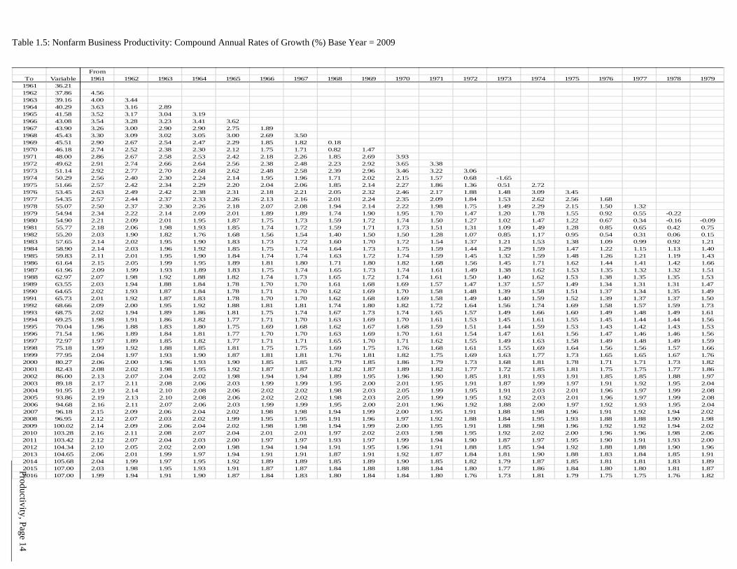
Table 1.5: Nonfarm Business Productivity: Compound Annual Rates of Growth (%) Base Year = 2009
FromTo Variable 1961 1962 1963 1964 1965 1966 1967 1968 1969 1970 1971 1972 1973 1974 1975 1976 1977 1978 1979
1961 36.211962 37.86 4.561963 39.16 4.00 3.441964 40.29 3.63 3.16 2.891965 41.58 3.52 3.17 3.04 3.191966 43.08 3.54 3.28 3.23 3.41 3.621967 43.90 3.26 3.00 2.90 2.90 2.75 1.891968 45.43 3.30 3.09 3.02 3.05 3.00 2.69 3.501969 45.51 2.90 2.67 2.54 2.47 2.29 1.85 1.82 0.181970 46.18 2.74 2.52 2.38 2.30 2.12 1.75 1.71 0.82 1.471971 48.00 2.86 2.67 2.58 2.53 2.42 2.18 2.26 1.85 2.69 3.931972 49.62 2.91 2.74 2.66 2.64 2.56 2.38 2.48 2.23 2.92 3.65 3.381973 51.14 2.92 2.77 2.70 2.68 2.62 2.48 2.58 2.39 2.96 3.46 3.22 3.061974 50.29 2.56 2.40 2.30 2.24 2.14 1.95 1.96 1.71 2.02 2.15 1.57 0.68 -1.651975 51.66 2.57 2.42 2.34 2.29 2.20 2.04 2.06 1.85 2.14 2.27 1.86 1.36 0.51 2.721976 53.45 2.63 2.49 2.42 2.38 2.31 2.18 2.21 2.05 2.32 2.46 2.17 1.88 1.48 3.09 3.451977 54.35 2.57 2.44 2.37 2.33 2.26 2.13 2.16 2.01 2.24 2.35 2.09 1.84 1.53 2.62 2.56 1.681978 55.07 2.50 2.37 2.30 2.26 2.18 2.07 2.08 1.94 2.14 2.22 1.98 1.75 1.49 2.29 2.15 1.50 1.321979 54.94 2.34 2.22 2.14 2.09 2.01 1.89 1.89 1.74 1.90 1.95 1.70 1.47 1.20 1.78 1.55 0.92 0.55 -0.221980 54.90 2.21 2.09 2.01 1.95 1.87 1.75 1.73 1.59 1.72 1.74 1.50 1.27 1.02 1.47 1.22 0.67 0.34 -0.16 -0.091981 55.77 2.18 2.06 1.98 1.93 1.85 1.74 1.72 1.59 1.71 1.73 1.51 1.31 1.09 1.49 1.28 0.85 0.65 0.42 0.751982 55.20 2.03 1.90 1.82 1.76 1.68 1.56 1.54 1.40 1.50 1.50 1.28 1.07 0.85 1.17 0.95 0.54 0.31 0.06 0.151983 57.65 2.14 2.02 1.95 1.90 1.83 1.73 1.72 1.60 1.70 1.72 1.54 1.37 1.21 1.53 1.38 1.09 0.99 0.92 1.211984 58.90 2.14 2.03 1.96 1.92 1.85 1.75 1.74 1.64 1.73 1.75 1.59 1.44 1.29 1.59 1.47 1.22 1.15 1.13 1.401985 59.83 2.11 2.01 1.95 1.90 1.84 1.74 1.74 1.63 1.72 1.74 1.59 1.45 1.32 1.59 1.48 1.26 1.21 1.19 1.431986 61.64 2.15 2.05 1.99 1.95 1.89 1.81 1.80 1.71 1.80 1.82 1.68 1.56 1.45 1.71 1.62 1.44 1.41 1.42 1.661987 61.96 2.09 1.99 1.93 1.89 1.83 1.75 1.74 1.65 1.73 1.74 1.61 1.49 1.38 1.62 1.53 1.35 1.32 1.32 1.511988 62.97 2.07 1.98 1.92 1.88 1.82 1.74 1.73 1.65 1.72 1.74 1.61 1.50 1.40 1.62 1.53 1.38 1.35 1.35 1.531989 63.55 2.03 1.94 1.88 1.84 1.78 1.70 1.70 1.61 1.68 1.69 1.57 1.47 1.37 1.57 1.49 1.34 1.31 1.31 1.471990 64.65 2.02 1.93 1.87 1.84 1.78 1.71 1.70 1.62 1.69 1.70 1.58 1.48 1.39 1.58 1.51 1.37 1.34 1.35 1.491991 65.73 2.01 1.92 1.87 1.83 1.78 1.70 1.70 1.62 1.68 1.69 1.58 1.49 1.40 1.59 1.52 1.39 1.37 1.37 1.501992 68.66 2.09 2.00 1.95 1.92 1.88 1.81 1.81 1.74 1.80 1.82 1.72 1.64 1.56 1.74 1.69 1.58 1.57 1.59 1.731993 68.75 2.02 1.94 1.89 1.86 1.81 1.75 1.74 1.67 1.73 1.74 1.65 1.57 1.49 1.66 1.60 1.49 1.48 1.49 1.611994 69.25 1.98 1.91 1.86 1.82 1.77 1.71 1.70 1.63 1.69 1.70 1.61 1.53 1.45 1.61 1.55 1.45 1.44 1.44 1.561995 70.04 1.96 1.88 1.83 1.80 1.75 1.69 1.68 1.62 1.67 1.68 1.59 1.51 1.44 1.59 1.53 1.43 1.42 1.43 1.531996 71.54 1.96 1.89 1.84 1.81 1.77 1.70 1.70 1.63 1.69 1.70 1.61 1.54 1.47 1.61 1.56 1.47 1.46 1.46 1.561997 72.97 1.97 1.89 1.85 1.82 1.77 1.71 1.71 1.65 1.70 1.71 1.62 1.55 1.49 1.63 1.58 1.49 1.48 1.49 1.591998 75.18 1.99 1.92 1.88 1.85 1.81 1.75 1.75 1.69 1.75 1.76 1.68 1.61 1.55 1.69 1.64 1.56 1.56 1.57 1.661999 77.95 2.04 1.97 1.93 1.90 1.87 1.81 1.81 1.76 1.81 1.82 1.75 1.69 1.63 1.77 1.73 1.65 1.65 1.67 1.762000 80.27 2.06 2.00 1.96 1.93 1.90 1.85 1.85 1.79 1.85 1.86 1.79 1.73 1.68 1.81 1.78 1.71 1.71 1.73 1.822001 82.43 2.08 2.02 1.98 1.95 1.92 1.87 1.87 1.82 1.87 1.89 1.82 1.77 1.72 1.85 1.81 1.75 1.75 1.77 1.862002 86.00 2.13 2.07 2.04 2.02 1.98 1.94 1.94 1.89 1.95 1.96 1.90 1.85 1.81 1.93 1.91 1.85 1.85 1.88 1.972003 89.18 2.17 2.11 2.08 2.06 2.03 1.99 1.99 1.95 2.00 2.01 1.95 1.91 1.87 1.99 1.97 1.91 1.92 1.95 2.042004 91.95 2.19 2.14 2.10 2.08 2.06 2.02 2.02 1.98 2.03 2.05 1.99 1.95 1.91 2.03 2.01 1.96 1.97 1.99 2.082005 93.86 2.19 2.13 2.10 2.08 2.06 2.02 2.02 1.98 2.03 2.05 1.99 1.95 1.92 2.03 2.01 1.96 1.97 1.99 2.082006 94.68 2.16 2.11 2.07 2.06 2.03 1.99 1.99 1.95 2.00 2.01 1.96 1.92 1.88 2.00 1.97 1.92 1.93 1.95 2.042007 96.18 2.15 2.09 2.06 2.04 2.02 1.98 1.98 1.94 1.99 2.00 1.95 1.91 1.88 1.98 1.96 1.91 1.92 1.94 2.022008 96.95 2.12 2.07 2.03 2.02 1.99 1.95 1.95 1.91 1.96 1.97 1.92 1.88 1.84 1.95 1.93 1.88 1.88 1.90 1.982009 100.02 2.14 2.09 2.06 2.04 2.02 1.98 1.98 1.94 1.99 2.00 1.95 1.91 1.88 1.98 1.96 1.92 1.92 1.94 2.022010 103.28 2.16 2.11 2.08 2.07 2.04 2.01 2.01 1.97 2.02 2.03 1.98 1.95 1.92 2.02 2.00 1.96 1.96 1.98 2.062011 103.42 2.12 2.07 2.04 2.03 2.00 1.97 1.97 1.93 1.97 1.99 1.94 1.90 1.87 1.97 1.95 1.90 1.91 1.93 2.002012 104.34 2.10 2.05 2.02 2.00 1.98 1.94 1.94 1.91 1.95 1.96 1.91 1.88 1.85 1.94 1.92 1.88 1.88 1.90 1.962013 104.65 2.06 2.01 1.99 1.97 1.94 1.91 1.91 1.87 1.91 1.92 1.87 1.84 1.81 1.90 1.88 1.83 1.84 1.85 1.912014 105.68 2.04 1.99 1.97 1.95 1.92 1.89 1.89 1.85 1.89 1.90 1.85 1.82 1.79 1.87 1.85 1.81 1.81 1.83 1.892015 107.00 2.03 1.98 1.95 1.93 1.91 1.87 1.87 1.84 1.88 1.88 1.84 1.80 1.77 1.86 1.84 1.80 1.80 1.81 1.872016 107.00 1.99 1.94 1.91 1.90 1.87 1.84 1.83 1.80 1.84 1.84 1.80 1.76 1.73 1.81 1.79 1.75 1.75 1.76 1.82
Productivity, Page 15
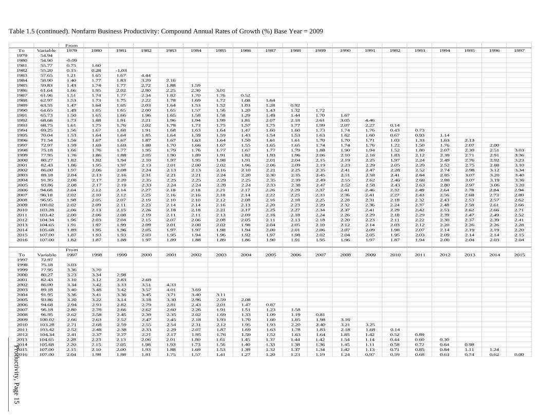
Table 1.5 (continued). Nonfarm Business Productivity: Compound Annual Rates of Growth (%) Base Year = 2009
FromTo Variable 1979 1980 1981 1982 1983 1984 1985 1986 1987 1988 1989 1990 1991 1992 1993 1994 1995 1996 1997
1979 54.941980 54.90 -0.091981 55.77 0.75 1.601982 55.20 0.15 0.28 -1.031983 57.65 1.21 1.65 1.67 4.441984 58.90 1.40 1.77 1.83 3.29 2.161985 59.83 1.43 1.74 1.77 2.72 1.88 1.591986 61.64 1.66 1.95 2.02 2.80 2.25 2.30 3.011987 61.96 1.51 1.74 1.77 2.34 1.82 1.70 1.76 0.521988 62.97 1.53 1.73 1.75 2.22 1.78 1.69 1.72 1.08 1.641989 63.55 1.47 1.64 1.65 2.03 1.64 1.53 1.52 1.03 1.28 0.921990 64.65 1.49 1.65 1.65 2.00 1.65 1.57 1.56 1.20 1.43 1.32 1.721991 65.73 1.50 1.65 1.66 1.96 1.65 1.58 1.58 1.29 1.49 1.44 1.70 1.671992 68.66 1.73 1.88 1.91 2.21 1.96 1.94 1.99 1.81 2.07 2.18 2.61 3.05 4.461993 68.75 1.61 1.75 1.76 2.02 1.78 1.73 1.75 1.57 1.75 1.77 1.99 2.07 2.27 0.141994 69.25 1.56 1.67 1.68 1.91 1.68 1.63 1.64 1.47 1.60 1.60 1.73 1.74 1.76 0.43 0.731995 70.04 1.53 1.64 1.64 1.85 1.64 1.59 1.59 1.43 1.54 1.53 1.63 1.62 1.60 0.67 0.93 1.141996 71.54 1.56 1.67 1.67 1.87 1.67 1.63 1.64 1.50 1.61 1.61 1.70 1.70 1.71 1.03 1.33 1.63 2.131997 72.97 1.59 1.69 1.69 1.88 1.70 1.66 1.67 1.55 1.65 1.65 1.74 1.74 1.76 1.22 1.50 1.76 2.07 2.001998 75.18 1.66 1.76 1.77 1.95 1.79 1.76 1.77 1.67 1.77 1.79 1.88 1.90 1.94 1.52 1.80 2.07 2.39 2.51 3.031999 77.95 1.76 1.86 1.88 2.05 1.90 1.89 1.91 1.82 1.93 1.96 2.06 2.10 2.16 1.83 2.12 2.39 2.71 2.91 3.362000 80.27 1.82 1.92 1.94 2.10 1.97 1.95 1.98 1.91 2.01 2.04 2.15 2.19 2.25 1.97 2.24 2.49 2.76 2.92 3.232001 82.43 1.86 1.95 1.97 2.13 2.01 2.00 2.02 1.96 2.06 2.09 2.19 2.23 2.29 2.05 2.29 2.52 2.75 2.88 3.102002 86.00 1.97 2.06 2.08 2.24 2.13 2.13 2.16 2.10 2.21 2.25 2.35 2.41 2.47 2.28 2.52 2.74 2.98 3.12 3.342003 89.18 2.04 2.13 2.16 2.31 2.21 2.21 2.24 2.20 2.30 2.35 2.45 2.51 2.58 2.41 2.64 2.85 3.07 3.20 3.402004 91.95 2.08 2.17 2.20 2.35 2.25 2.25 2.29 2.25 2.35 2.39 2.49 2.55 2.62 2.46 2.68 2.88 3.07 3.19 3.362005 93.86 2.08 2.17 2.19 2.33 2.24 2.24 2.28 2.24 2.33 2.38 2.47 2.52 2.58 2.43 2.63 2.80 2.97 3.06 3.202006 94.68 2.04 2.12 2.14 2.27 2.18 2.18 2.21 2.17 2.26 2.29 2.37 2.41 2.46 2.32 2.49 2.64 2.78 2.84 2.942007 96.18 2.02 2.10 2.12 2.25 2.16 2.16 2.18 2.14 2.22 2.25 2.33 2.36 2.41 2.27 2.43 2.56 2.68 2.73 2.802008 96.95 1.98 2.05 2.07 2.19 2.10 2.10 2.12 2.08 2.16 2.18 2.25 2.28 2.31 2.18 2.32 2.43 2.53 2.57 2.622009 100.02 2.02 2.09 2.11 2.23 2.14 2.14 2.16 2.13 2.20 2.23 2.29 2.32 2.36 2.24 2.37 2.48 2.58 2.61 2.662010 103.28 2.06 2.13 2.15 2.26 2.18 2.18 2.21 2.17 2.25 2.27 2.34 2.37 2.41 2.29 2.42 2.53 2.62 2.66 2.712011 103.42 2.00 2.06 2.08 2.19 2.11 2.11 2.13 2.09 2.16 2.18 2.24 2.26 2.29 2.18 2.29 2.39 2.47 2.49 2.522012 104.34 1.96 2.03 2.04 2.15 2.07 2.06 2.08 2.05 2.11 2.13 2.18 2.20 2.23 2.11 2.22 2.30 2.37 2.39 2.412013 104.65 1.91 1.97 1.99 2.09 2.01 2.00 2.02 1.98 2.04 2.05 2.10 2.12 2.14 2.03 2.12 2.20 2.26 2.26 2.282014 105.68 1.89 1.95 1.96 2.05 1.97 1.97 1.98 1.94 2.00 2.01 2.06 2.07 2.09 1.98 2.07 2.14 2.19 2.19 2.202015 107.00 1.87 1.93 1.93 2.03 1.95 1.94 1.96 1.92 1.97 1.98 2.02 2.04 2.05 1.95 2.03 2.09 2.14 2.14 2.152016 107.00 1.82 1.87 1.88 1.97 1.89 1.88 1.89 1.86 1.90 1.91 1.95 1.96 1.97 1.87 1.94 2.00 2.04 2.03 2.04
FromTo Variable 1997 1998 1999 2000 2001 2002 2003 2004 2005 2006 2007 2008 2009 2010 2011 2012 2013 2014 2015
1997 72.971998 75.18 3.031999 77.95 3.36 3.702000 80.27 3.23 3.34 2.982001 82.43 3.10 3.12 2.83 2.692002 86.00 3.34 3.42 3.33 3.51 4.332003 89.18 3.40 3.48 3.42 3.57 4.01 3.692004 91.95 3.36 3.41 3.36 3.45 3.71 3.40 3.112005 93.86 3.20 3.22 3.14 3.18 3.30 2.96 2.59 2.082006 94.68 2.94 2.93 2.82 2.79 2.81 2.43 2.01 1.47 0.872007 96.18 2.80 2.78 2.66 2.62 2.60 2.26 1.91 1.51 1.23 1.582008 96.95 2.62 2.58 2.45 2.39 2.35 2.02 1.69 1.33 1.09 1.19 0.812009 100.02 2.66 2.63 2.52 2.47 2.45 2.18 1.93 1.70 1.60 1.85 1.98 3.162010 103.28 2.71 2.68 2.59 2.55 2.54 2.31 2.12 1.95 1.93 2.20 2.40 3.21 3.252011 103.42 2.52 2.48 2.38 2.33 2.29 2.07 1.87 1.69 1.63 1.78 1.83 2.18 1.68 0.142012 104.34 2.41 2.37 2.27 2.21 2.17 1.95 1.76 1.59 1.52 1.63 1.64 1.85 1.42 0.52 0.892013 104.65 2.28 2.23 2.13 2.06 2.01 1.80 1.61 1.45 1.37 1.44 1.42 1.54 1.14 0.44 0.60 0.302014 105.68 2.20 2.15 2.05 1.98 1.93 1.73 1.56 1.40 1.33 1.38 1.36 1.45 1.11 0.58 0.72 0.64 0.982015 107.00 2.15 2.10 2.00 1.93 1.88 1.69 1.53 1.39 1.32 1.37 1.34 1.42 1.13 0.71 0.85 0.84 1.11 1.242016 107.00 2.04 1.98 1.88 1.81 1.75 1.57 1.41 1.27 1.20 1.23 1.19 1.24 0.97 0.59 0.68 0.63 0.74 0.62 0.00
Productivity, Page 16
1.5 Appendix Nordhaus demonstrates how the growth rates in productivity in n sectors of the economy can be aggregated to the growth rate in total-economy productivity.21 Monaco adopts the formulation to aggregate the growth rates in productivity in the nonfarm business, farm, and “all other” sectors.22 Equation A1 is a similar adaptation to five sectors: nonfarm business (n), farm (f), households (h), nonprofit institutions (i), and general government (g).
)wt(wtH)wt(wtH
)wt(wtH)wt(wtH)wt(wtH
wtPwtPwtPwtPwtPP(A1)
Hg
Qgg
Hi
Qii
Hh
Qhh
Hf
Qff
Hn
Qnn
Qgg
Qii
Qhh
Qff
Qnnt
−+−
+−+−+−
+++++=
••
•••
••••••
Where, ▪
X = rate of change in x P = productivity H = hours worked wtQ
f = nominal output weight for farm sector defined as the ratio of nominal GDP in the farm sector to nominal GDP for the total economy
wtHf = hours worked weight for farm sector defined as the ratio of hours worked
in the farm sector to hours worked in the total economy t = total economy In the long-range, it is reasonable to assume that the growth rate in hours worked in all sectors will be equal. Thus, Equation A1 can be simplified to A2.
Qgg
Qii
Qhh
Qff
Qnnt wtPwtPwtPwtPwtPP(A2)
••••••
++++=
Furthermore, if the ultimate long-range growth rates in productivity in the household, nonprofits, and general government sectors are zero, Equation A2 can be further simplified to A3.
Qff
Qnnt wtPwtPP(A3)
•••
+=
21 Nordhaus, William D., “Productivity Growth and the New Economy.” Brookings Papers on Economic Activity, (Volume 2, 2002). pp.211-265
22 Monaco, Ralph, “Issues in Projecting Productivity in the Very Long Term.” Sept. 28, 2005. Treasury Office of Economic Policy. Unpublished.
Price Inflation, Page 1
2. PRICE INFLATION THE 2018 TRUSTEES REPORT
OFFICE OF THE CHIEF ACTUARY, SOCIAL SECURITY ADMINISTRATION TABLE OF CONTENTS PAGE 2 PRICE INFLATION .............................................................................................................. 2
2.1 SUMMARY ...................................................................................................................................................... 2 2.2 CONSUMER PRICE INDEX FOR URBAN WAGE EARNERS AND CLERICAL WORKERS (CPI-W) ......................... 3
2.2.1 Historical Growth in the Adjusted CPI-W ............................................................................................. 3 2.2.2 Future Growth in the CPI-W ................................................................................................................. 4 2.2.3 Recent and Expected Future Changes to Methods BLS Uses to Compute the CPI................................ 5 2.2.4 OCACT Adjustments to the Published CPI-W ....................................................................................... 6
2.3 PRICE DIFFERENTIAL ...................................................................................................................................... 6 2.3.1 Computational Methods for Price Measures ......................................................................................... 7 2.3.2 Coverage Differences ............................................................................................................................ 8 2.3.3 Future Expectations for the Price Differential .................................................................................... 10
2.4 GROSS DOMESTIC PRODUCT IMPLICIT PRICE DEFLATOR (PGDP) ................................................................ 11 2.4.1 Historical Behavior of the Adjusted PGDP ......................................................................................... 11
2.4.1.1 Adjusted Deflator for Personal Consumption Expenditures (PGDP_C) .......................................................... 11 2.4.1.2 Deflator for Investment Expenditures (PGDP_I) ............................................................................................. 12 2.4.1.3 Deflator for Government Expenditures (PGDP_G) ......................................................................................... 16
2.4.2 Recent BEA Changes to PGDP............................................................................................................ 17 2.4.3 OCACT Adjustments to the Published PGDP ...................................................................................... 17
2.5 PROJECTIONS FROM OTHER SOURCES ........................................................................................................... 18 2.6 APPENDIX ..................................................................................................................................................... 23
TABLE OF TABLES PAGE TABLE 2.1: ASSUMED ULTIMATE ANNUAL RATES OF INCREASE IN PRICE LEVEL MEASURES ....................................... 2 TABLE 2.2: HISTORICAL GROWTH IN THE ADJUSTED CPI-W ......................................................................................... 4 TABLE 2.3: ESTIMATED CONTRIBUTION TO THE PRICE DIFFERENTIAL ........................................................................... 9 TABLE 2.4: ADJUSTED CPI-W: COMPOUND ANNUAL RATES OF GROWTH (%) BASE YEAR = 1982-1984 .................... 19 TABLE 2.5: ADJUSTED GDP DEFLATOR: COMPOUND ANNUAL RATES OF GROWTH (%) BASE YEAR = 2009 .............. 21
Price Inflation, Page 2
2 Price Inflation
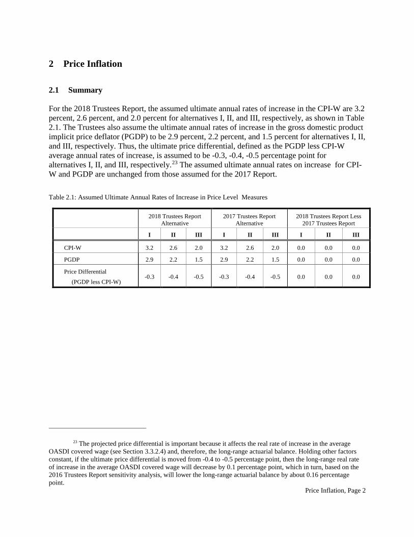
2.1 Summary For the 2018 Trustees Report, the assumed ultimate annual rates of increase in the CPI-W are 3.2 percent, 2.6 percent, and 2.0 percent for alternatives I, II, and III, respectively, as shown in Table 2.1. The Trustees also assume the ultimate annual rates of increase in the gross domestic product implicit price deflator (PGDP) to be 2.9 percent, 2.2 percent, and 1.5 percent for alternatives I, II, and III, respectively. Thus, the ultimate price differential, defined as the PGDP less CPI-W average annual rates of increase, is assumed to be -0.3, -0.4, -0.5 percentage point for alternatives I, II, and III, respectively.23 The assumed ultimate annual rates on increase for CPI-W and PGDP are unchanged from those assumed for the 2017 Report.
Table 2.1: Assumed Ultimate Annual Rates of Increase in Price Level Measures
2018 Trustees Report Alternative
2017 Trustees Report Alternative
2018 Trustees Report Less 2017 Trustees Report
I II III I II III I II III
CPI-W 3.2 2.6 2.0 3.2 2.6 2.0 0.0 0.0 0.0
PGDP 2.9 2.2 1.5 2.9 2.2 1.5 0.0 0.0 0.0
Price Differential
(PGDP less CPI-W) -0.3 -0.4 -0.5 -0.3 -0.4 -0.5 0.0 0.0 0.0
23 The projected price differential is important because it affects the real rate of increase in the average OASDI covered wage (see Section 3.3.2.4) and, therefore, the long-range actuarial balance. Holding other factors constant, if the ultimate price differential is moved from -0.4 to -0.5 percentage point, then the long-range real rate of increase in the average OASDI covered wage will decrease by 0.1 percentage point, which in turn, based on the 2016 Trustees Report sensitivity analysis, will lower the long-range actuarial balance by about 0.16 percentage point.
Price Inflation, Page 3
2.2 Consumer Price Index for Urban Wage Earners and Clerical Workers (CPI-W)
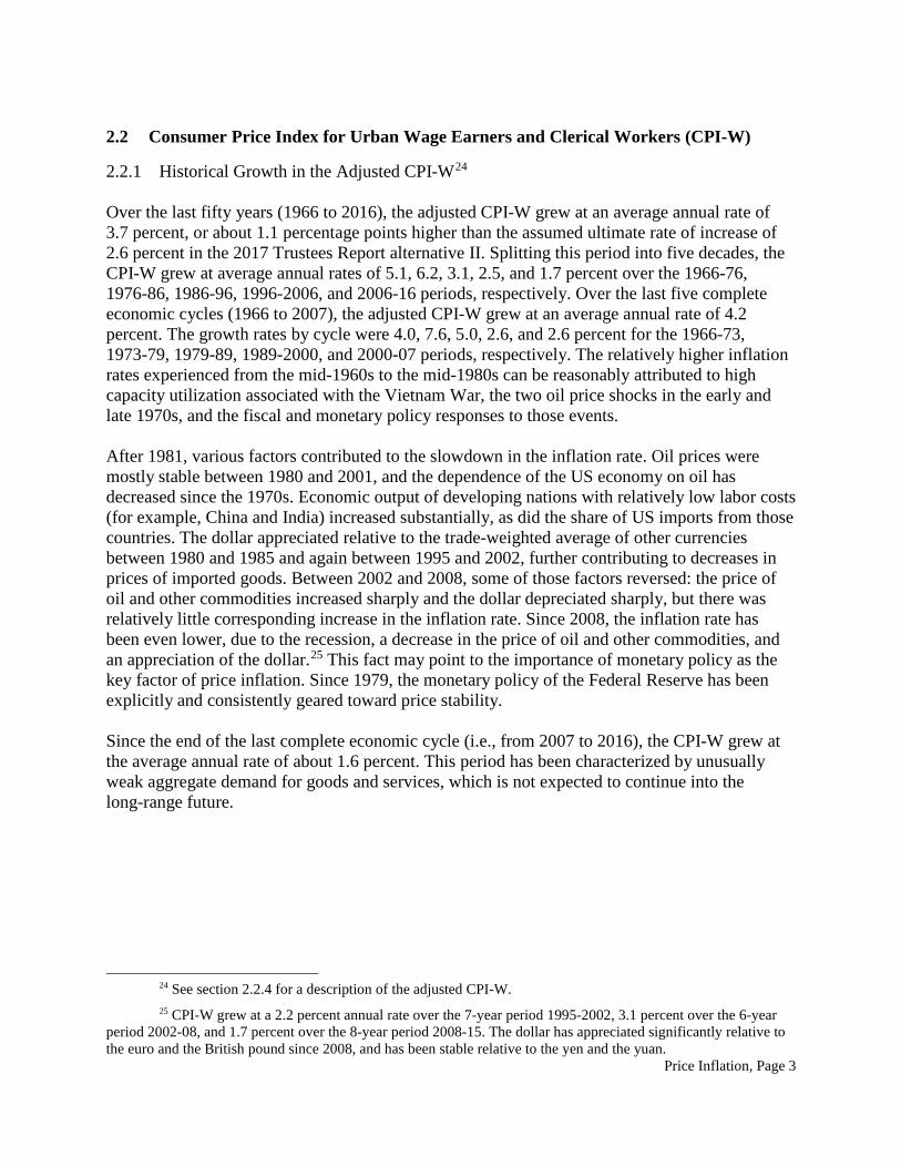
2.2.1 Historical Growth in the Adjusted CPI-W24 Over the last fifty years (1966 to 2016), the adjusted CPI-W grew at an average annual rate of 3.7 percent, or about 1.1 percentage points higher than the assumed ultimate rate of increase of 2.6 percent in the 2017 Trustees Report alternative II. Splitting this period into five decades, the CPI-W grew at average annual rates of 5.1, 6.2, 3.1, 2.5, and 1.7 percent over the 1966-76, 1976-86, 1986-96, 1996-2006, and 2006-16 periods, respectively. Over the last five complete economic cycles (1966 to 2007), the adjusted CPI-W grew at an average annual rate of 4.2 percent. The growth rates by cycle were 4.0, 7.6, 5.0, 2.6, and 2.6 percent for the 1966-73, 1973-79, 1979-89, 1989-2000, and 2000-07 periods, respectively. The relatively higher inflation rates experienced from the mid-1960s to the mid-1980s can be reasonably attributed to high capacity utilization associated with the Vietnam War, the two oil price shocks in the early and late 1970s, and the fiscal and monetary policy responses to those events. After 1981, various factors contributed to the slowdown in the inflation rate. Oil prices were mostly stable between 1980 and 2001, and the dependence of the US economy on oil has decreased since the 1970s. Economic output of developing nations with relatively low labor costs (for example, China and India) increased substantially, as did the share of US imports from those countries. The dollar appreciated relative to the trade-weighted average of other currencies between 1980 and 1985 and again between 1995 and 2002, further contributing to decreases in prices of imported goods. Between 2002 and 2008, some of those factors reversed: the price of oil and other commodities increased sharply and the dollar depreciated sharply, but there was relatively little corresponding increase in the inflation rate. Since 2008, the inflation rate has been even lower, due to the recession, a decrease in the price of oil and other commodities, and an appreciation of the dollar.25 This fact may point to the importance of monetary policy as the key factor of price inflation. Since 1979, the monetary policy of the Federal Reserve has been explicitly and consistently geared toward price stability. Since the end of the last complete economic cycle (i.e., from 2007 to 2016), the CPI-W grew at the average annual rate of about 1.6 percent. This period has been characterized by unusually weak aggregate demand for goods and services, which is not expected to continue into the long-range future.
24 See section 2.2.4 for a description of the adjusted CPI-W. 25 CPI-W grew at a 2.2 percent annual rate over the 7-year period 1995-2002, 3.1 percent over the 6-year
period 2002-08, and 1.7 percent over the 8-year period 2008-15. The dollar has appreciated significantly relative to the euro and the British pound since 2008, and has been stable relative to the yen and the yuan.
Price Inflation, Page 4
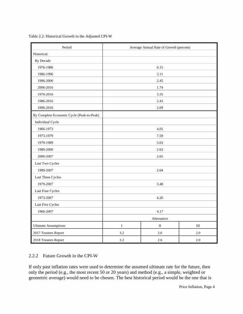
Table 2.2: Historical Growth in the Adjusted CPI-W
Period Average Annual Rate of Growth (percent)
Historical:
By Decade
1976-1986 6.15
1986-1996 3.11
1996-2006 2.45
2006-2016 1.74
1976-2016 3.35
1986-2016 2.43
1996-2016 2.09
By Complete Economic Cycle (Peak-to-Peak)
Individual Cycle
1966-1973 4.05
1973-1979 7.59
1979-1989 5.03
1989-2000 2.63
2000-2007 2.65
Last Two Cycles
1989-2007 2.64
Last Three Cycles
1979-2007 3.48
Last Four Cycles
1973-2007 4.20
Last Five Cycles
1966-2007 4.17
Alternative
Ultimate Assumptions I II III
2017 Trustees Report 3.2 2.6 2.0
2018 Trustees Report 3.2 2.6 2.0
2.2.2 Future Growth in the CPI-W If only past inflation rates were used to determine the assumed ultimate rate for the future, then only the period (e.g., the most recent 50 or 20 years) and method (e.g., a simple, weighted or geometric average) would need to be chosen. The best historical period would be the one that is
Price Inflation, Page 5
most representative of the conditions that are expected to prevail over the upcoming 75-year projection period. The 50-year historical record is filled with inflation-related events, some of which occurred in unique circumstances and have limited relevance for projecting the future. These may include the Vietnam War, oil price shocks, and periods of price controls. Furthermore, after a historically unusual departure in the 1970s, monetary policy has returned to a strong emphasis on price stability. While these specific historical events will not recur in the future (at least not exactly as they have in the past), other inflation-related events may take their place. It is reasonable to expect some additional upward pressure on the future growth rate in the CPI due to changes in international trade. The ratio of net exports (i.e., exports less imports) to GDP averaged about -3.5 percent over the 10-year period from 2007 through 2016. Part of this imbalance is due to imports of relatively low-priced consumer goods from emerging markets, such as China. However, as these developing economies mature, their average wage and consumption are expected to rise relative to their output, and their currencies and price levels are expected to rise relative to those of the U.S. This may put further upward pressure on the prices of basic commodities and, therefore, the CPI. These trends are also expected to ultimately return the ratio of net exports to GDP to zero in the future. The 3.7 percent average annual growth rate for the adjusted CPI-W for the 50-year period from 1966 to 2016 is probably higher than the most reasonable assumption for the ultimate CPI-W annual rate of increase. OCACT believes that the 2.6 percent average annual growth rate for the adjusted CPI-W over the last two complete economic cycles (as measured over an 18-year period from 1989 to 2007), a period that reflects the current domestic monetary policy environment expected to exist in the future, is more representative of an expected future trend. Thus, the assumed ultimate rate of increase in the CPI-W is 2.6 percent for alternative II, and 3.2 and 2.0 percent for alternatives I and III, respectively.
2.2.3 Recent and Expected Future Changes to Methods BLS Uses to Compute the CPI The Bureau of Labor Statistics (BLS) collects and publishes data on the CPI. BLS updated the consumption expenditure weights in the CPI-W and in the CPI for all Urban Consumers (CPI-U) from the 2011-2012 to 2013-2014 period, effective January 2016.26 Since 2000, BLS has been updating the weights every two years, and plans to continue on that schedule, instead of the pre-2000 historical average of about once per decade. BLS believes that more frequent updates of the consumption-expenditure weights will have little or no effect on the average future growth rate in the CPI over long periods.27 Recent data support this view for relatively short periods. When BLS switched from using 1999-2000 to 2001-2002 weights beginning in January 2004, it
26 For BLS’s CPI methodology, see http://www.bls.gov/opub/hom/pdf/homch17.pdf. The new weights are in http://www.bls.gov/cpi/usri_2015.txt, and the weights they replaced are in http://www.bls.gov/cpi/usri11-12_2015.pdf. Unlike in previous years, BLS made no special note of the change in their January 2016 news release.
27 Future Schedule for Expenditure Weight Updates in the Consumer Price Index, BLS, http://stats.bls.gov/cpi/cpiupdt.htm.
Price Inflation, Page 6
published monthly values for the CPI-W (and CPI-U) for January through June 2004 based on the 1999-2000 expenditure weights.28 The values in June 2004 for the CPI-W (and CPI-U) based on the old and new weights were identical. However, the data may also vary over short periods. When BLS switched from using 2001-2002 to 2003-2004 weights beginning in January 2006, it published monthly values for the CPI-W (and CPI-U) for January through June 2006 based on the 2001-2002 expenditure weights.29 The data indicate that the growth rate in the CPI-W (and CPI-U) over this period was about 0.2 percentage point lower using the newer weights. 30
2.2.4 OCACT Adjustments to the Published CPI-W Over the years, BLS has introduced numerous improvements to the CPI-W. For example, beginning in January 1995 and July 1996, BLS introduced changes to correct methodological errors introduced into the index in January 1978 and January 1987. In addition, beginning in January 1999, BLS introduced a new geometric mean formula that assumes some lower-level substitution among items purchased by consumers within broad categories of goods and services due to changes in relative prices. Since BLS has no plans to revise the historical CPI, these improvements present a comparability problem. The goal is to project future growth rates in the CPI, based, in part, on an analysis of historical growth rates. Any projected growth rate in the CPI will be affected by the BLS method improvements mentioned above. Thus, OCACT adjusted the historical CPI to reflect the estimated effects of these method changes, effectively reducing the measured growth rate in the CPI-W over the historical period. This adjustment is the same as in last year’s Trustees Report. Table 2.4 lists the adjusted CPI-W. (See Section 2.6 Appendix for details on OCACT’s adjustments to the actual published CPI-W annual growth rates.)
2.3 Price Differential The Bureau of Economic Analysis (BEA) publishes values for the PGDP in its National Income and Product Accounts (NIPA). The price differential is defined as the annual growth rate in the PGDP less the annual growth rate in the CPI-W. The price differential exists mostly due to differences in computational methods and, to a lesser degree, coverage differences between the CPI-W and the PGDP. For the 2018 Trustees Report alternative II, the assumed ultimate price differential is -0.4 percentage point, which is equal to the sum of -0.3 percentage point due to the difference in computational methods and -0.1 percentage point due to coverage differences.
28 News Release for Consumer Price Index, January through June 2004, BLS, Table 1(OW) and Table 2(OW), http://stats.bls.gov/schedule/archives/cpi_nr.htm.
29 News Release for Consumer Price Index, January through June 2006, BLS, Table 1(OW) and Table 2(OW), http://stats.bls.gov/schedule/archives/cpi_nr.htm.
30 This was partly due to the fact that, compared to the old 2001-2002 weight, the new 2003-2004 weight for gasoline fell by about 0.2 percentage point while the price of gasoline rose by about 25.0 percent from January to June 2006.
Price Inflation, Page 7
Over the 10-year complete economic cycle from 1979 to 1989, the average annual growth rates in the PGDP and the adjusted CPI-W were 4.68 and 5.03 percent, respectively, resulting in a price differential of -0.35 percentage point (i.e., approximately 4.68 less 5.03). Over the next complete economic cycle, an 11-year period from 1989 to 2000, the average annual growth rates in the PGDP and the adjusted CPI-W were 2.20 and 2.63 percent, respectively, resulting in a price differential of -0.43 percentage point (i.e., approximately 2.20 less 2.63). Over the latest complete economic cycle, a 7-year period from 2000 to 2007, the average annual growth rates in the PGDP and the adjusted CPI-W were 2.50 and 2.65 percent, respectively, so the price differential averaged only -0.15 percentage point. It is reasonable to believe this experience was an aberration due to highly unusual price changes in areas where coverage is different between the CPI-W and the PGDP. In particular, prices of exports and imports are far more volatile than prices of goods and services produced and consumed domestically, and the price differential over any short period can be greatly influenced by the volatility of export and import prices. The average annual price differential over the 9-year period from 2007 to 2016 was -0.10 percentage point.31
2.3.1 Computational Methods for Price Measures32 Prior to August 2002, BLS announced that it would produce an additional monthly price index based on the CPI-U using an alternative chained formula for combining prices across broad categories of goods and services.33 This measure (C-CPI-U) is designed to reflect changes in the distribution of consumer expenditures across these broad groups as they occur during each month. The CPI-U (as well as the CPI-W) reflects a static distribution of consumer expenditures on a monthly basis, adjusting the static distribution every two years. BLS simulated a C-CPI-U for the 1990 to 1995 period and estimated that the average annual growth rate in the C-CPI-U would have been 0.15 percentage point lower than the actual published CPI-U for the period. Based in part on this value, the Trustees assumed a 0.2 percentage point difference in the future ultimate average annual growth rates for the PGDP and CPI-W (i.e., a -0.2 price differential) in the 2000, 2001, and 2002 Trustees Reports. In August 2002, BLS began publishing monthly values for the C-CPI-U. BLS also improved and extended its simulation of the C-CPI-U and estimated that the average annual growth rate in the C-CPI-U would have been lower by 0.22 (instead of 0.15) percentage point over the 1990 to 1995 period, 0.43 percentage point over the 1996 to 1999 period, and 0.30 percentage point over
31 This value is greatly influenced by a large decrease in export and import prices in 2015-16. If those last
two years are excluded, the average price differential over the 7-year period from 2007 to 2014 was -0.38 percentage points.
32 By convention, the computational effect and price differential are expressed in positive and negative terms, respectively. For example, a computational effect of 0.3 percentage point will, by itself, contribute -0.3 percentage point to the price differential.
33 Note on a New, Supplemental Index of Consumer Price Change, BLS, http://stats.bls.gov/cpi/cpisuptn.htm.
Price Inflation, Page 8
the combined 1990 to 1999 period.34 Based in part on these higher values, the Trustees increased the assumed difference in the future ultimate average annual growth rates for the PGDP and CPI-W from 0.2 to 0.3 percentage point (i.e., a change from a -0.2 to -0.3 price differential) for the 2003, 2004, and 2005 Trustees Reports. Actual final monthly values for the C-CPI-U are now available back to December 1999.35 One can directly calculate the difference between the static and chained computational methods for the latest periods as the CPI-U less C-CPI-U annual growth rates. The average annual difference over the period from December 1999 to December 2015 was 0.27, and the differences for the 12-month periods ending each December ranged from -0.1 to 0.8 percentage points. In 13 out of the 16 years, the difference was between 0.1 and 0.5 percentage points. It is reasonable to believe that some of the difference between these computational methods in the more recent period may have been due to unique circumstances associated with price volatility in particular items such as energy, and thus that the difference between these two computational methods may be lower in the future. However, for the post-1999 period, the average annual difference using the all items less food and energy expenditure category for the C-CPI-U and CPI-U was 0.31 percent, very close to the value for the all items category.36 Summarizing the BLS data, the difference in growth in the CPI-U and the C-CPI-U was about 0.3 percentage point over the 1990 to 1999 period and about 0.3 percentage point over the period from December 1999 to December 2015. This suggests that the difference in measured growth in prices in the CPI-U and the C-CPI-U is likely to average about 0.3 percentage point in the future.
2.3.2 Coverage Differences The CPI-W covers the consumption pattern for roughly 28 percent of the U.S. population.37 The PGDP covers the consumption expenditures for the entire population, along with investment and government expenditures.38 In fact, the PGDP can be viewed as a weighted average of deflators
34Simulated CPI-U compared to simulated C-CPI-U: U.S. city average, All-items, December indexes relative to previous December, BLS, http://stats.bls.gov/cpi/superchart2.htm.
35 Because the C-CPI-U is dependent upon expenditure data that lag the CPI release date, BLS publishes initial, interim, and final monthly values for each calendar year. As of October 2017, final values were available through September 2016.
36 Using the all items less food and energy expenditure category for the C-CPI-U and CPI-U, the difference between the static and the chained computational methods was 0.7 percentage point in 2000 (compared to 0.8 using the all items category). For subsequent years, the difference was 0.6 (0.3), 0.3 (0.4), 0.4 (0.2), -0.1 (0.1), 0.3 (0.5), 0.4 (0.3), 0.5 (0.4), 0.0 (-0.1), 0.3 (0.3), 0.2 (0.2), 0.0 (0.0), 0.3 (0.3), 0.2 (0.2), 0.4 (0.2) and 0.4 (0.3) percentage point for 12-month periods ending in December 2001, 2002, 2003, 2004, 2005, 2006, 2007, 2008, 2009, 2010, 2011, 2012, 2013 2014, and 2015, respectively.
37 Overview of the CPI, BLS. http://stats.bls.gov/cpi/cpifaq.htm#Question_3. 38 The PGDP also incorporates the effect of price changes in exports less the effect of price changes in
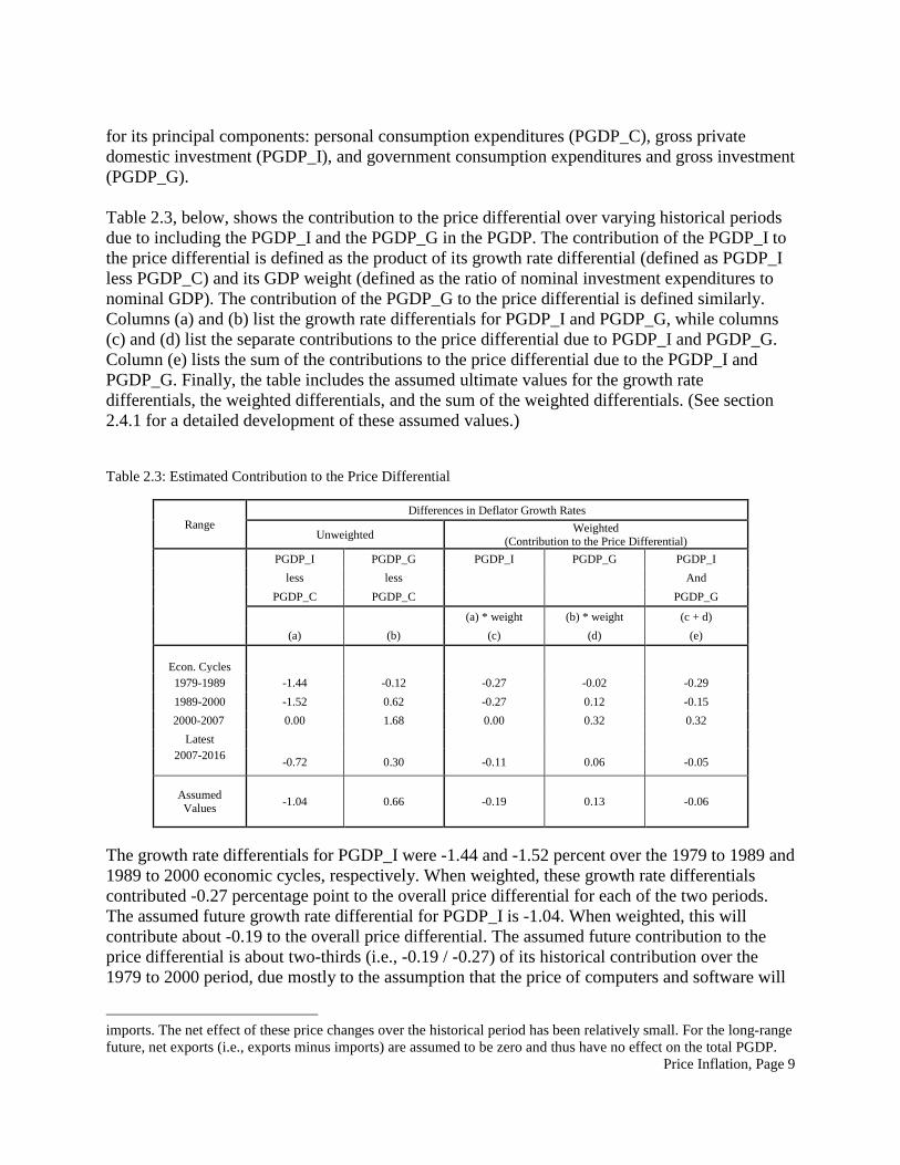
Price Inflation, Page 9
for its principal components: personal consumption expenditures (PGDP_C), gross private domestic investment (PGDP_I), and government consumption expenditures and gross investment (PGDP_G). Table 2.3, below, shows the contribution to the price differential over varying historical periods due to including the PGDP_I and the PGDP_G in the PGDP. The contribution of the PGDP_I to the price differential is defined as the product of its growth rate differential (defined as PGDP_I less PGDP_C) and its GDP weight (defined as the ratio of nominal investment expenditures to nominal GDP). The contribution of the PGDP_G to the price differential is defined similarly. Columns (a) and (b) list the growth rate differentials for PGDP_I and PGDP_G, while columns (c) and (d) list the separate contributions to the price differential due to PGDP_I and PGDP_G. Column (e) lists the sum of the contributions to the price differential due to the PGDP_I and PGDP_G. Finally, the table includes the assumed ultimate values for the growth rate differentials, the weighted differentials, and the sum of the weighted differentials. (See section 2.4.1 for a detailed development of these assumed values.) Table 2.3: Estimated Contribution to the Price Differential
Range Differences in Deflator Growth Rates
Unweighted Weighted (Contribution to the Price Differential)
PGDP_I PGDP_G PGDP_I PGDP_G PGDP_I less less And PGDP_C PGDP_C PGDP_G
(a) * weight (b) * weight (c + d) (a) (b) (c) (d) (e)
Econ. Cycles
1979-1989 -1.44 -0.12 -0.27 -0.02 -0.29 1989-2000 -1.52 0.62 -0.27 0.12 -0.15
2000-2007 0.00 1.68 0.00 0.32 0.32 Latest
2007-2016 -0.72 0.30 -0.11 0.06 -0.05
Assumed Values -1.04 0.66 -0.19 0.13 -0.06
The growth rate differentials for PGDP_I were -1.44 and -1.52 percent over the 1979 to 1989 and 1989 to 2000 economic cycles, respectively. When weighted, these growth rate differentials contributed -0.27 percentage point to the overall price differential for each of the two periods. The assumed future growth rate differential for PGDP_I is -1.04. When weighted, this will contribute about -0.19 to the overall price differential. The assumed future contribution to the price differential is about two-thirds (i.e., -0.19 / -0.27) of its historical contribution over the 1979 to 2000 period, due mostly to the assumption that the price of computers and software will
imports. The net effect of these price changes over the historical period has been relatively small. For the long-range future, net exports (i.e., exports minus imports) are assumed to be zero and thus have no effect on the total PGDP.
Price Inflation, Page 10
not fall as steeply in the long-range future compared to the post-1979 historical period. The 7-year period from 2000 to 2007 was discounted on the belief that the behavior of the PGDP_I during this period was an aberration. The growth rate differential for PGDP_I was 0.0 percent during this period due to the relatively rapid growth in the investment deflators for residential and nonresidential structures. This trend is not sustainable and thus unlikely to continue into future. In fact, the growth rate differential for PGDP_I turned back to an average annual value of -0.72 percent for the 9-year period from 2007 to 2016, reflecting, in part, actual declines in the price of new housing in most markets during the first half of that period. The growth rate differentials for PGDP_G were -0.12 and 0.62 percent over the 1979 to 1989 and 1989 to 2000 economic cycles, respectively. When weighted, these growth rate differentials contributed -0.02 and 0.12 percentage point to the overall price differential for those periods. The assumed future growth rate differential for PGDP_G is 0.66, which when weighted will contribute about 0.13 to the overall price differential. The assumed future contribution to the price differential is about 0.08 higher (i.e., 0.13 – 0.05) than its historical contribution over the 1979 to 2000 period. The PGDP_G contribution to the price differential during this historical period was temporarily depressed due to a relative increase in lower-paid state and local government workers. The PGDP_G contribution to the price differential during the 7-year period from 2000 to 2007 was high because of the unusually high growth rate in average military compensation, averaging 9.2 percent over the period. OCACT believes this relatively high growth rate was due to temporary factors. Federal payments for basic military pay, reenlistment bonuses, and other types of incentive pay increased sharply after the 9/11 terrorist attacks. Furthermore, beginning in 2002, the BEA redefined military compensation to include federal payments to the Uniformed Services Retiree Healthcare Fund. In the future, the OCACT believes that the annual growth rate in average military compensation will slow and follow the assumed ultimate 3.9 percent average annual growth rate in compensation for all workers. The assumed future contribution to the price differential due to the PGDP_I and the PGDP_G is -0.1 percentage point. This is approximately equal to the rounded sum of a -0.19 percentage point price differential due to the PGDP_I and 0.13 percentage point price differential due to the PGDP_G. The assumed future combined contribution of -0.1 percentage point is smaller (less negative) than the actual average annual historical combined contribution to the price differential of -0.21 percentage point over the 1979 to 2000 period.
2.3.3 Future Expectations for the Price Differential For the 2018 Trustees Report, the assumed ultimate price differential is -0.3, -0.4, and -0.5 percentage point for alternative I, II, and III, respectively. For the alternative II, the ultimate price differential of -0.4 percentage point is the sum of -0.3 percentage point due to the difference in computational methods and -0.1 percentage point due to coverage differences between the PGDP and CPI-W. These values are unchanged from the ones used in the 2017 Report.
Price Inflation, Page 11
2.4 Gross Domestic Product Implicit Price Deflator (PGDP)
2.4.1 Historical Behavior of the Adjusted PGDP As mentioned in section 2.3.2, for the future, the PGDP can be viewed as a weighted average of the PGDP_C, PGDP_I, and PGDP_G. The weights are the ratios of the components’ nominal expenditures to total nominal GDP. In 2016, the weights for personal consumption, investment, and government expenditures were about 0.69, 0.16, and 0.18, respectively. These weights summed to more than one because net exports were negative. However, the net exports in the long-range future are assumed to be zero and, hence, the weights are assumed to add up to 1.0. Because these weights have been relatively stable over the last four decades (and have summed to about 1.0), the long-run historical growth rate in PGDP is mostly explained by the separate historical growth rates in PGDP_C, PGDP_I, and PGDP_G. The historical and expected future growth rates for each component deflator are examined below.
2.4.1.1 Adjusted Deflator for Personal Consumption Expenditures (PGDP_C) Given all of the changes to the CPI and PGDP over time, it seems reasonable to expect that the more recent decades best depict the future relationship between the two price measures; more specifically, only the post-1977 period when the adjusted CPI-W incorporates most of the methodological improvements in the CPI as presently defined. Over the 37-year period from 1979 to 2016, the average annual growth rates for the adjusted PGDP_C and adjusted CPI-W were 2.81 and 3.02 percent, respectively. Hence, the difference between these average annual growth rates over this period was about -0.21 percentage point (i.e., 2.81 − 3.02). This -0.21 percentage point observed difference over the 1979 to 2016 period is somewhat smaller (less negative) than the -0.30 percentage point expected future difference (consistent with the estimated 0.30 percentage point difference due to the computational methods used for weighting broad groups of goods and services). Some differences between the two quantities can be expected because the populations covered by the two price measures are different. As mentioned in Section 2.3.2, the CPI-W covers the consumption pattern for roughly 32 percent of the population, while the PGDP_C covers personal consumption expenditures for the total population. The CPI-U, on the other hand, covers about 89 percent of the population. Over the 1979 to 2016 period, the CPI-U grew faster than the CPI-W by about 0.09 percentage point per year, mostly because of relatively larger weights for medical and college expenditures—two areas where prices had been rising faster than for other goods. If the CPI-W had the same expenditure weights as the CPI-U, then the adjusted CPI-W would have grown at an annual rate of roughly 0.09 percentage point faster than it did. This would have resulted in an observed difference (adjusted PGDP_C less adjusted CPI-W growth rates) of -0.30 (i.e., -0.21 − 0.09) percentage point, which is equal to the -0.30 percentage point expected difference due to computational methods alone. The most recently revised BLS and BEA data for 2000 and later also support a 0.30 percentage point effect for the different computational methods (adjusted PGDP_C less adjusted CPI-W
Price Inflation, Page 12
growth rates). As mentioned in Section 2.3.1, BLS has published initial, interim, and final monthly values for the C-CPI-U for each year beginning January 2000. Final values are now available for 2015. The average annual growth rate in the C-CPI-U from the first quarter of 2000 to the fourth quarter of 2015 was 1.88 percent. Over the same period, the average annual growth rates in the PGDP_C, CPI-U, and CPI-W were approximately 1.83, 2.12, and 2.11 percent, respectively. The data suggest that over this period, the contribution of the difference in computational methods was about 0.24 percentage point (i.e., 2.12 − 1.88), and that the PGDP_C price differential was -0.28 percentage point (i.e., 1.83 − 2.11).39 Over the long-range period, it is reasonable to assume that the average annual growth rates in the CPI-W and CPI-U will be roughly equal. It also seems reasonable to assume that the difference in the long-range average annual growth rates (PGDP_C less CPI-W) will be -0.30 percentage point, and that this difference will be only due to the expected 0.30 percentage point effect from the different computational weighting methods. Stated differently, the expected growth-rate differential for the personal consumption deflator (PGDP_C less CPI-W) due to factors other than from the computational weighting methods is assumed to be zero. Thus, the assumed ultimate annual growth rate for PGDP_C is 2.3 percent, equal to the assumed ultimate annual growth rate for CPI-W (i.e., 2.6 percent) less the 0.30 percentage point effect of the different computational weighting methods.
2.4.1.2 Deflator for Investment Expenditures (PGDP_I) The PGDP_I can be viewed as a weighted average of deflators for its principal components: investment in equipment (PGDP_INE), investment in intellectual property (PGDP_INIP), residential investment (PGDP_IR), and investment in nonresidential structures (PGDP_INS).40 The equipment and intellectual property components in their current form were first used in the 2013 revisions to NIPA.
Deflator for Equipment (PGDP_INE) – Over the 37-year period from 1979 to 2016, the average annual growth rate was about 0.12 percent for the PGDP_INE, compared to 2.81 percent for the PGDP_C. The PGDP_INE growth rate has been depressed by the rise in nominal investment expenditures for computers and the sharp decline in their quality-adjusted prices. Over this period, the deflator for computers fell at an average annual rate of about 12.03 percent, and the ratio of nominal investment expenditures for computers to all investment expenditures for equipment rose from about 5 percent to about 13 percent in the late 1990s, followed by a decline to about 7 percent in 2016.
39 The data also suggest that over the period the average annual growth rate in the C-CPI-U (1.88 percent)
was a reasonable approximation of the average annual growth rate in the PGDP_C (1.83 percent), and that the average annual growth rates in the CPI-U (2.12 percent) and CPI-W (2.11 percent) were approximately equal over the period, compared to the 0.09 average annual percentage point differential (CPI-U minus CPI-W) over the 1979-2016 period.
40 This decomposition excludes the change in business inventories, which has averaged roughly 1.7 percent
of total investment expenditures over the 37-year period from 1979 to 2016.
Price Inflation, Page 13
It seems reasonable to assume that quality-adjusted computer prices will continue to decline into the future, but at a somewhat slower rate. The average annual rate of decline was about 12.9 percent over the 1982 to 1994 period, 22.2 percent over the 1994 to 1999 period, and 7.6 percent over the 1999 to 2016 period. The large rate of decline in the late 1990s was probably due to a combination of technological advances and production volume increases that are unlikely to be sustained over a longer period. It seems more reasonable to assume that the future rate of price decline will be similar to that over the last 17 years; thus, the assumed rate of decline in quality-adjusted computer prices is 8 percent per year. Furthermore, it is expected that the ratio of nominal investment expenditures for computers to all investment expenditures for equipment will stabilize at the approximate average value of the ratio over the last decade (i.e., 10 percent). Over the period from 1979 to 2016, the deflator for equipment other than computers grew on average at a 1.58 percent annual rate, or 1.23 percentage points less than the 2.81 percent annual growth rate for the PGDP_C. Similarly, over the last three complete economic cycles (1979-2007), the deflator for other equipment grew slower by 1.33 percentage points per year than PGDP_C. OCACT believes that the growth rate in the price deflator for other equipment will continue to be depressed relative to the PGDP_C, since the prices for at least some items in other equipment (e.g., printers, calculators, etc.) will be driven down by the same types of future technological advancements expected for computers. Thus, it is reasonable to expect that, in the future, the average annual growth rate in other equipment will be about 1.05 percent, or 1.25 percentage points less than the 2.3 percent assumed ultimate average annual growth rate in the PGDP_C. Using these average annual growth rates and weights, OCACT believes that it is reasonable to set the assumed ultimate average annual rate of growth in PGDP_INE in the future to about 0.15 percent (i.e., -8.0 * 0.10 + 1.05 * 0.90). Deflator for Intellectual Property (PGDP_INIP) – Over the 37-year period from 1979 to 2016, the average annual growth rate was about 1.51 percent for the PGDP_INIP, compared to 2.81 percent for the PGDP_C. The PGDP_INIP growth rate has been depressed by the rise in nominal investment expenditures for software and a slow but steady decline in its quality-adjusted prices. Over this period, the deflator for software fell at an average annual rate of about 0.94 percent, and the ratio of nominal investment expenditures for software to all investment expenditures for intellectual property rose from about 17 percent to about 45 percent by 2000, and has slowly increased to about 47 percent since. Software prices have been declining slowly, but steadily. They declined over four of the last five economic cycles (the only exception being the 1973-79 cycle), and their rate of decline averaged between 0 and 1 percent per year over three of those four cycles. (The rate of decline over the 1989-2000 cycle was 1.9 percent per year.) Since the end of the last cycle (a 9-year period from 2007 to 2016), software prices declined at an average annual rate of 0.24 percent. It seems reasonable to expect some future price decline, but at a somewhat slower rate than the average over the last 37 years. OCACT expects that software prices will decline at a rate of 0.5 percent per year. OCACT also expects that the ratio of nominal investment expenditures for software to all investment expenditures for intellectual property will stabilize at about 45 percent.
Price Inflation, Page 14
Over the period from 1979 to 2016, the deflator for intellectual property other than software grew on average at a 2.53 percent annual rate, or 0.28 percentage point less than the 2.81 percent annual growth rate for the PGDP_C. Over the last three complete economic cycles (1979-2007), the deflator for other intellectual property grew at an annual rate of 3.05 percent, slower by 0.19 percentage point per year than the 3.24 percent growth rate in PGDP_C. OCACT believes that it is reasonable to expect that, in the future, the average annual growth rate in the price deflator for other intellectual property will continue to be somewhat lower than the PGDP_C. The assumed growth rate in the deflator for other intellectual property is 2.1 percent, or 0.2 percentage point less than the 2.3 percent assumed ultimate average annual growth rate in the PGDP_C. Using these average annual growth rates and weights, OCACT believes that it is reasonable to set the assumed ultimate average annual rate of growth in PGDP_INIP in the future to about 0.88 percent (i.e., -0.5 * 0.47 + 2.1 * 0.53).
Deflator for Residential Investment (PGDP_IR) – Residential investment is almost entirely composed of investment in fixed structures, which, in turn, is composed of single-family, multifamily, and other structures (e.g., manufactured homes, dormitories, etc.). Over the 21-year period from 1979 to 2000, the average annual growth rate was about 3.75 percent for the PGDP_IR, compared to 3.58 percent for the PGDP_C. Thus, the average annual growth rate for the PGDP_IR was about 0.17 percentage point (3.75 − 3.58) higher than the average annual growth rate in the PGDP_C over the period. However, over the next 7-year period, this differential increased substantially. From 2000 to 2007, the average annual growth rate was about 4.73 percent for the PGDP_IR and 2.24 percent for the PGDP_C. Thus, the average annual growth rate for the PGDP_IR was about 2.49 percentage points (4.73 – 2.24) higher than the average annual growth rate in the PGDP_C over the period. OCACT believes that the 2.49 percent growth rate differential between the PGDP_IR and the PGDP_C over the last business cycle was a temporary market phenomenon characterized by overheated demand for housing, house “flipping,” subprime mortgage lending, and unusually high profits and gains in stock prices for the builders of new homes. Since 2007, there has been a market correction: the housing bubble has collapsed, new and existing home sales have dropped nationally, prices of new homes in most markets have declined, and the profits and stock prices of new homebuilders have plummeted. Although the housing market has been recovering lately, home prices in 2016 were still below the 2006 level, and the number of sales is well below the mid-2000s level. For the 2007 to 2016 period, the average annual growth in PGDP_IR and PGDP_C was 1.49 and 1.48 percent, respectively, indicating a 0,01 percent (1.49 − 1.48) differential between the two deflators. Over the 16-year period from 2000 to 2016, the average annual growth rate for the PGDP_IR was about 2.90 percent, or 1.09 percentage points higher than the 1.81 percent annual growth rate for the PGDP_C.
Price Inflation, Page 15
OCACT believes it is reasonable to disregard the post-2000 period and set the assumed ultimate average annual rate of increase in the PGDP_IR to 2.5 percent, or about 0.2 percentage point higher than the 2.3 percent assumed ultimate average annual rate of increase in the PGDP_C. 41 Deflator for Investment in Nonresidential Structures (PGDP_INS) – Investment in nonresidential structures includes investment in structures used for drilling for petroleum and natural gas. Over the 21-year period from 1979 to 2000, the average annual growth rate for PGDP_INS was 3.62 percent, or slightly less than the 3.75 percent growth rate in PGDP_IR. However, over the 7-year period from 2000 to 2007, the average annual growth rates for PGDP_INS and PGDP_IR were 7.29 and 4.73 percent, respectively. The relatively faster average annual growth rate for PGDP_INS occurred because the average annual growth rate in the deflator for investment in petroleum and natural gas was about 20.9 percent. Excluding the effects of petroleum and natural gas, the average annual growth rate for PGDP_INS was about 6.4 percent, closer to the 4.7 percent average annual growth rate in PGDP_IR over the period. OCACT believes the relatively rapid growth rate in the deflator for investment in petroleum and natural gas is a temporary market phenomenon associated with a run-up in oil prices. The price of a barrel of oil rose from about $26 in 2001 to $72 in 2007, or at an average annual rate of about 19.0 percent. As the market price for oil rose, previously expensive technologies became economically profitable. OCACT believes that in the future the average annual growth rate in the price of a barrel of oil will not be significantly greater than the growth rate in the PGDP_C and that the average annual growth rates in the PGDP_INS and PGDP_IR will be approximately equal. Thus, the assumed ultimate average annual rate of increase in PGDP_INS is 2.5 percent, or 0.2 percentage point higher than the 2.3 percent assumed ultimate average annual growth rate in the PGDP_C, and equal to the assumed ultimate average annual rate of increase in the PGDP_IR.
The ratio of investment expenditures in equipment to total investment expenditures has been stable over the past 60 years, averaging about 36 percent, so it is reasonable to assume that level will continue to hold in the future. Investment in intellectual property has been an increasing share of total investment. Much of the increase, however, has been due to the sharp rise in investment in software from the 1970s to the early 2000s. Since the share of software in the investment in intellectual property has stabilized recently, OCACT believes it is reasonable to assume that the ratio of investment in intellectual property to total investment will be similar to its recent levels, or about 24 percent. OCACT also assumes that the investment expenditure weights for nonresidential investment for structures and residential investment will account for approximately equal shares of the rest of the investment expenditures, or 20 percent each. Thus, the assumed ultimate average annual rate of increase for PGDP_I is 1.26 percent (i.e., 0.15 * 0.36 + 0.88 * 0.24 + 2.5 * (0.20 + 0.20)).
41 In the future, the PGDP_IR may grow faster than the PGDP_C due to more rapid increases in the prices
of scarce land and basic building commodities such as copper, lumber, and cement.
Price Inflation, Page 16
2.4.1.3 Deflator for Government Expenditures (PGDP_G) The PGDP_G can be viewed as a weighted average of deflators for government consumption expenditures (PGDP_GC) and government investment (PGDP_GI). Deflator for Government Consumption Expenditures (PGDP_GC) – Government consumption expenditures can be separated into employee compensation and other (residual) government consumption expenditures. In the NIPA, the deflator for government consumption expenditures on employee compensation is defined as average employee compensation. From 1979 to 2000, a 21-year period covering two complete economic cycles, the average annual growth rate in the deflator for employee compensation and the adjusted CPI-W were about 5.34 and 3.76 percent, respectively. This indicates that over the period, the real annual growth rate in average employee compensation was 1.58 percentage points (i.e., 5.34 – 3.76), slightly higher than the assumed ultimate real annual growth rate in average compensation in the 2017 Trustees Report.42 From 2000 to 2007, a 7-year period covering the latest economic cycle, the average annual growth rate in the deflator for employee compensation and the adjusted CPI-W were about 4.90 and 2.65 percent, respectively. This indicates that over the period, the real annual growth rate in average government compensation was 2.25 percentage points (i.e., 4.90 − 2.65), about a percentage point higher than the 1.27 percent ultimate real annual growth rate in average compensation assumed in the 2017 Trustees Report. OCACT believes that the relatively high growth rate in the deflator for employee compensation over the 2000 to 2007 period is a temporary phenomenon mostly associated with military pay incentives related to the conflicts in Iraq and Afghanistan. Over this period, the average annual growth rates in the average compensation of state and local, federal civilian, and federal military employees were 4.34, 5.50, and 9.21 percent, respectively. By contrast, between 2007 and 2016, the average annual growth rates in the average compensation of state and local, federal civilian, and federal military employees were 2.55, 2.60, and 1.73 percent, respectively, and the average annual growth rate in the deflator for employee compensation was 2.53 percent, or just 0.92 percentage points higher than the 1.61 percent growth rate in CPI-W over the same period. It is reasonable to assume that in the future the average annual growth rate in the average compensation for all government employees will be 3.87 percent, the same rate assumed for the economy-wide average compensation. Therefore, OCACT believes that the average annual growth rate in the deflator for government consumption expenditures on employee compensation will be 3.87 percent.43
42 For the 2017 Trustees Report alternative II, the Trustees assumed that the ultimate average annual rates
of increase in the average compensation for all employees and in the CPI were 3.87 and 2.6 percent, respectively. 43 For the 2018 Report, OCACT assumes the size of the active military remains constant throughout the
projection period, rather than increasing proportionally with the civilian employment. This implies a gradual shift in weights between civilian government employment and the military and, since the average military compensation is higher, a slightly slower average growth in government compensation. However, the effect is small.
Price Inflation, Page 17
It is also reasonable and consistent to assume that the average annual growth rate in the deflator for other government consumption will be equal to the assumed ultimate average annual growth rate in the PGDP_C, or 2.3 percent. Using rough averages over the 1979 to 2016 period, OCACT assumes that future government consumption expenditures for employee compensation will be about 70 percent of total government consumption expenditures. Thus, the assumed ultimate average annual growth rate for PGDP_GC is 3.40 percent (i.e., 3.87 * 0.70 + 2.3 * 0.30). Deflator for Government Investment (PGDP_GI) – Government investment can be separated into 1) structures, 2) equipment, and 3) intellectual property. It is reasonable to assume that the future average annual growth rate in the deflator for each of these categories of government investment will be equal to the expected future average annual growth rate in the corresponding categories of private. Thus, OCACT also assumes the future average annual growth rates in the deflator for government investment will be 2.5 percent for investment in structures, 0.15 percent for investment in equipment, and 0.88 percent for investment in intellectual property. Using rough averages over the 1979 to 2016 period, OCACT assumes the future ratio of government investment components to total government investment will be about 0.45 for structures, about 0.25 for equipment, and about 0.30 for intellectual property. Thus, the assumed ultimate average annual growth rate for PGDP_GI is 1.42 percent (i.e., 2.5 * 0.45 + 0.15 * 0.25 + 0.88 * 0.30). Finally, the historical proportions of government consumption and investment expenditures have been relatively stable over the 40-year period from 1976 to 2016, averaging about 78 and 22 percent of total government expenditures, respectively. Hence, the assumed ultimate average annual rate of increase in the PGDP_G is 2.96 percent (i.e., 3.4 * 0.78 + 1.42 * 0.22).
2.4.2 Recent BEA Changes to PGDP On July 28, 2017, BEA released a regular annual revision to the NIPA affecting the estimates for 2014 and later.44 Compared to previously published values, BEA increased the level of the PGDP by a negligible amount for 2014, and by 0.01 percentage point for 2015. These changes do not warrant any adjustment to the assumed future values.
2.4.3 OCACT Adjustments to the Published PGDP BEA’s estimate of the PGDP is based, in part, on BLS’s estimate of the CPI. BLS has introduced numerous improvements to the CPI that have lowered its post-1995 growth rate. BEA “backcasted” these improvements in the NIPA, lowering the growth rate in the PGDP (and raising the real growth rate in GDP). However, because BEA only backcasted these effects to 1978, OCACT has lowered the pre-1978 growth rate in the PGDP for consistency (see Section
44 https://bea.gov/newsreleases/national/gdp/2017/gdp2q17_adv.htm.
Price Inflation, Page 18
2.6 Appendix for further details on the adjustments to the actual published annual growth rates in PGDP and annual real growth rates in GDP). The adjusted PGDP is shown in Table 2.5.
2.5 Projections from Other Sources IHS Markit (formerly Global Insight, Inc.) provides projections through 2047 in its latest long-run trend forecast (see The 30-Year Focus, Third Quarter, August 2017). Over the 20-year period from 2027 to 2047, IHS Markit projects an average annual rate of increase of 2.40 percent for the CPI and 2.06 percent for the PGDP, with a resulting price differential of -0.34 percentage point (2.06 − 2.40). The Moody’s Analytics’ September 2017 forecast extends to 2047. Over the 20-year period from 2027 to 2047, Moody’s Analytics projects an average annual growth rate of 2.37 percent for the CPI and 1.98 percent for the PGDP, for a price differential of -0.39 percentage point (1.98 – 2.37). The Office of Management and Budget (OMB) Mid-Session Review of the Fiscal Year 2018 Budget includes projections through 2027. OMB’s annual growth rates for the PGDP and CPI-W (and CPI-U) for 2027 were 2.00 and 2.26 percent, respectively. Thus, OMB projects a price differential of -0.26 percentage point (i.e., 2.00 – 2.26). The Congressional Budget Office (CBO) March 2017 report, The 2017 Long-Term Budget Outlook, includes projections through 2047. CBO’s annual growth rates for the PGDP and CPI-W (and CPI-U) for 2027-47 were 2.0 and 2.4 percent, respectively. Thus, CBO projects an average annual price differential of -0.4 percentage point (i.e., 2.0 − 2.4) for the period. The Social Security Advisory Board’s 2015 Technical Panel on Assumptions and Methods recommended assuming an ultimate (i.e., long-range average) annual rate of increase in the CPI-W of 2.5 percent for alternative II, and a price differential of -0.4 percentage point.
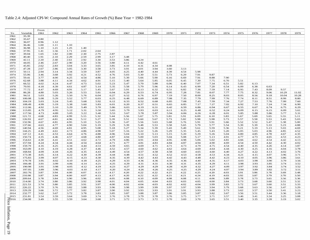
Price Inflation, Page 19
Table 2.4: Adjusted CPI-W: Compound Annual Rates of Growth (%) Base Year = 1982-1984
FromTo Variable 1961 1962 1963 1964 1965 1966 1967 1968 1969 1970 1971 1972 1973 1974 1975 1976 1977 1978 1979
1961 35.391962 35.67 0.801963 36.07 0.96 1.121964 36.46 1.00 1.11 1.101965 36.98 1.10 1.21 1.25 1.401966 37.95 1.41 1.56 1.71 2.02 2.641967 39.04 1.65 1.82 2.00 2.30 2.75 2.871968 40.40 1.91 2.10 2.29 2.59 2.99 3.17 3.481969 42.11 2.20 2.40 2.61 2.92 3.30 3.53 3.86 4.241970 44.05 2.46 2.67 2.90 3.20 3.56 3.80 4.11 4.42 4.611971 45.85 2.62 2.83 3.04 3.33 3.65 3.85 4.10 4.31 4.34 4.081972 47.28 2.67 2.86 3.05 3.30 3.58 3.73 3.91 4.01 3.94 3.60 3.131973 50.11 2.94 3.14 3.34 3.59 3.87 4.05 4.25 4.40 4.44 4.39 4.54 5.981974 55.06 3.46 3.68 3.92 4.21 4.52 4.76 5.03 5.30 5.51 5.73 6.29 7.91 9.871975 59.41 3.77 4.00 4.25 4.54 4.86 5.10 5.39 5.66 5.90 6.16 6.69 7.91 8.88 7.901976 62.68 3.88 4.11 4.34 4.62 4.91 5.15 5.40 5.64 5.85 6.05 6.45 7.30 7.75 6.70 5.511977 66.52 4.02 4.24 4.47 4.73 5.02 5.23 5.47 5.70 5.88 6.06 6.40 7.07 7.34 6.51 5.82 6.131978 70.93 4.18 4.39 4.61 4.87 5.14 5.35 5.58 5.79 5.96 6.14 6.43 6.99 7.20 6.54 6.09 6.38 6.631979 77.72 4.47 4.69 4.91 5.17 5.45 5.67 5.91 6.13 6.32 6.51 6.82 7.36 7.59 7.14 6.95 7.43 8.09 9.571980 86.28 4.80 5.03 5.26 5.53 5.81 6.04 6.29 6.53 6.74 6.95 7.28 7.81 8.07 7.77 7.75 8.32 9.06 10.29 11.021981 94.51 5.03 5.26 5.50 5.76 6.04 6.27 6.52 6.76 6.97 7.19 7.50 8.00 8.25 8.03 8.05 8.56 9.18 10.04 10.281982 100.08 5.08 5.29 5.52 5.77 6.03 6.25 6.48 6.69 6.89 7.08 7.35 7.79 7.99 7.76 7.74 8.11 8.51 8.99 8.801983 104.19 5.03 5.24 5.45 5.68 5.92 6.12 6.33 6.52 6.68 6.85 7.08 7.45 7.59 7.34 7.27 7.53 7.76 7.99 7.601984 108.49 4.99 5.19 5.38 5.60 5.83 6.01 6.20 6.37 6.51 6.65 6.85 7.17 7.27 7.02 6.92 7.10 7.24 7.34 6.901985 112.06 4.92 5.10 5.29 5.49 5.70 5.86 6.03 6.19 6.31 6.42 6.59 6.86 6.94 6.67 6.55 6.67 6.74 6.75 6.291986 113.85 4.79 4.95 5.12 5.31 5.50 5.65 5.79 5.93 6.03 6.11 6.25 6.48 6.52 6.24 6.09 6.15 6.15 6.09 5.611987 117.56 4.73 4.89 5.05 5.22 5.40 5.53 5.67 5.78 5.87 5.94 6.06 6.26 6.28 6.01 5.85 5.88 5.86 5.77 5.311988 121.72 4.68 4.83 4.99 5.15 5.32 5.44 5.56 5.67 5.75 5.81 5.91 6.09 6.10 5.83 5.67 5.69 5.65 5.55 5.111989 126.93 4.67 4.81 4.96 5.12 5.27 5.39 5.51 5.60 5.67 5.73 5.82 5.98 5.98 5.73 5.57 5.58 5.53 5.43 5.031990 132.96 4.67 4.81 4.95 5.10 5.25 5.36 5.47 5.56 5.63 5.68 5.76 5.91 5.91 5.66 5.52 5.52 5.47 5.38 5.001991 137.66 4.63 4.77 4.90 5.04 5.19 5.29 5.39 5.48 5.53 5.58 5.65 5.79 5.77 5.54 5.39 5.39 5.33 5.23 4.881992 140.94 4.56 4.69 4.81 4.95 5.08 5.18 5.27 5.34 5.39 5.43 5.49 5.61 5.59 5.36 5.21 5.19 5.13 5.03 4.691993 144.25 4.49 4.61 4.73 4.86 4.98 5.07 5.16 5.22 5.26 5.29 5.35 5.45 5.43 5.20 5.05 5.03 4.96 4.85 4.521994 147.12 4.41 4.53 4.64 4.76 4.88 4.96 5.04 5.10 5.13 5.15 5.20 5.29 5.26 5.04 4.89 4.85 4.78 4.67 4.351995 150.74 4.35 4.46 4.57 4.68 4.80 4.87 4.94 5.00 5.03 5.04 5.08 5.17 5.13 4.91 4.77 4.73 4.65 4.53 4.231996 154.63 4.30 4.41 4.51 4.62 4.72 4.79 4.86 4.91 4.94 4.95 4.98 5.06 5.02 4.81 4.66 4.62 4.54 4.42 4.131997 157.94 4.24 4.34 4.44 4.54 4.64 4.71 4.77 4.81 4.83 4.84 4.87 4.94 4.90 4.69 4.54 4.50 4.42 4.30 4.021998 159.79 4.16 4.25 4.34 4.44 4.53 4.59 4.65 4.69 4.71 4.71 4.73 4.79 4.75 4.54 4.40 4.35 4.26 4.14 3.871999 163.09 4.10 4.19 4.28 4.37 4.46 4.52 4.57 4.60 4.62 4.62 4.64 4.69 4.64 4.44 4.30 4.25 4.16 4.04 3.782000 168.84 4.09 4.18 4.26 4.35 4.43 4.49 4.54 4.57 4.58 4.58 4.60 4.65 4.60 4.40 4.27 4.22 4.13 4.02 3.762001 173.38 4.05 4.14 4.22 4.30 4.39 4.44 4.48 4.51 4.52 4.52 4.53 4.58 4.53 4.34 4.21 4.15 4.07 3.96 3.712002 175.83 3.99 4.07 4.15 4.23 4.30 4.35 4.39 4.42 4.43 4.42 4.43 4.48 4.42 4.23 4.10 4.05 3.96 3.86 3.612003 179.78 3.95 4.02 4.10 4.18 4.25 4.29 4.33 4.36 4.36 4.35 4.36 4.40 4.35 4.17 4.03 3.98 3.90 3.79 3.562004 184.48 3.91 3.99 4.06 4.14 4.21 4.25 4.29 4.31 4.31 4.30 4.31 4.35 4.29 4.11 3.98 3.93 3.85 3.74 3.522005 190.98 3.91 3.98 4.05 4.12 4.19 4.23 4.27 4.29 4.29 4.28 4.29 4.32 4.27 4.09 3.97 3.92 3.84 3.74 3.522006 197.05 3.89 3.96 4.03 4.10 4.17 4.20 4.24 4.26 4.26 4.25 4.25 4.29 4.24 4.07 3.94 3.89 3.82 3.72 3.512007 202.76 3.87 3.94 4.00 4.07 4.13 4.17 4.20 4.22 4.22 4.21 4.22 4.25 4.20 4.03 3.91 3.86 3.78 3.69 3.482008 210.98 3.87 3.94 4.00 4.07 4.13 4.17 4.20 4.22 4.22 4.21 4.21 4.24 4.19 4.03 3.92 3.87 3.79 3.70 3.502009 209.64 3.78 3.84 3.90 3.96 4.02 4.05 4.08 4.10 4.09 4.08 4.08 4.11 4.06 3.89 3.78 3.73 3.65 3.56 3.362010 214.00 3.74 3.80 3.86 3.92 3.98 4.01 4.04 4.05 4.04 4.03 4.03 4.05 4.00 3.84 3.73 3.68 3.60 3.51 3.322011 221.53 3.74 3.80 3.85 3.91 3.97 4.00 4.02 4.04 4.03 4.02 4.02 4.04 3.99 3.83 3.72 3.67 3.60 3.51 3.332012 226.22 3.70 3.76 3.82 3.88 3.93 3.96 3.98 3.99 3.99 3.97 3.97 3.99 3.94 3.79 3.68 3.63 3.56 3.47 3.292013 229.29 3.66 3.72 3.77 3.82 3.87 3.90 3.92 3.93 3.93 3.91 3.91 3.93 3.88 3.73 3.62 3.57 3.50 3.41 3.232014 232.77 3.62 3.67 3.72 3.78 3.83 3.85 3.87 3.88 3.87 3.86 3.85 3.87 3.82 3.67 3.56 3.51 3.44 3.36 3.182015 231.81 3.54 3.59 3.64 3.69 3.74 3.76 3.78 3.79 3.78 3.76 3.75 3.77 3.71 3.57 3.46 3.41 3.34 3.25 3.082016 234.08 3.49 3.55 3.59 3.64 3.68 3.71 3.72 3.73 3.72 3.70 3.69 3.70 3.65 3.51 3.40 3.35 3.28 3.19 3.02
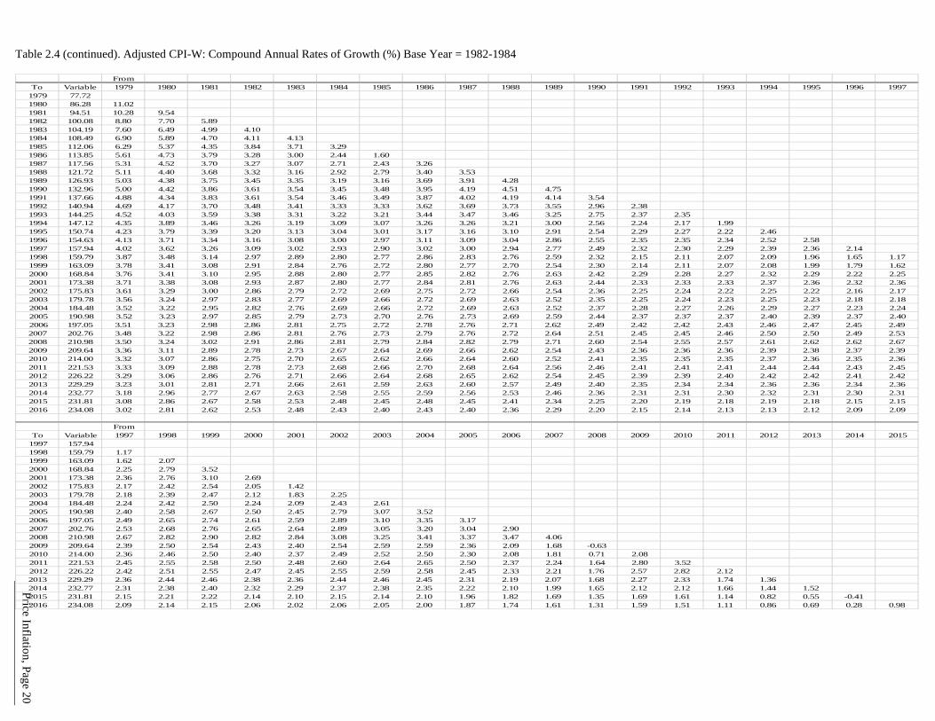
Price Inflation, Page 20
Table 2.4 (continued). Adjusted CPI-W: Compound Annual Rates of Growth (%) Base Year = 1982-1984
FromTo Variable 1979 1980 1981 1982 1983 1984 1985 1986 1987 1988 1989 1990 1991 1992 1993 1994 1995 1996 1997
1979 77.721980 86.28 11.021981 94.51 10.28 9.541982 100.08 8.80 7.70 5.891983 104.19 7.60 6.49 4.99 4.101984 108.49 6.90 5.89 4.70 4.11 4.131985 112.06 6.29 5.37 4.35 3.84 3.71 3.291986 113.85 5.61 4.73 3.79 3.28 3.00 2.44 1.601987 117.56 5.31 4.52 3.70 3.27 3.07 2.71 2.43 3.261988 121.72 5.11 4.40 3.68 3.32 3.16 2.92 2.79 3.40 3.531989 126.93 5.03 4.38 3.75 3.45 3.35 3.19 3.16 3.69 3.91 4.281990 132.96 5.00 4.42 3.86 3.61 3.54 3.45 3.48 3.95 4.19 4.51 4.751991 137.66 4.88 4.34 3.83 3.61 3.54 3.46 3.49 3.87 4.02 4.19 4.14 3.541992 140.94 4.69 4.17 3.70 3.48 3.41 3.33 3.33 3.62 3.69 3.73 3.55 2.96 2.381993 144.25 4.52 4.03 3.59 3.38 3.31 3.22 3.21 3.44 3.47 3.46 3.25 2.75 2.37 2.351994 147.12 4.35 3.89 3.46 3.26 3.19 3.09 3.07 3.26 3.26 3.21 3.00 2.56 2.24 2.17 1.991995 150.74 4.23 3.79 3.39 3.20 3.13 3.04 3.01 3.17 3.16 3.10 2.91 2.54 2.29 2.27 2.22 2.461996 154.63 4.13 3.71 3.34 3.16 3.08 3.00 2.97 3.11 3.09 3.04 2.86 2.55 2.35 2.35 2.34 2.52 2.581997 157.94 4.02 3.62 3.26 3.09 3.02 2.93 2.90 3.02 3.00 2.94 2.77 2.49 2.32 2.30 2.29 2.39 2.36 2.141998 159.79 3.87 3.48 3.14 2.97 2.89 2.80 2.77 2.86 2.83 2.76 2.59 2.32 2.15 2.11 2.07 2.09 1.96 1.65 1.171999 163.09 3.78 3.41 3.08 2.91 2.84 2.76 2.72 2.80 2.77 2.70 2.54 2.30 2.14 2.11 2.07 2.08 1.99 1.79 1.622000 168.84 3.76 3.41 3.10 2.95 2.88 2.80 2.77 2.85 2.82 2.76 2.63 2.42 2.29 2.28 2.27 2.32 2.29 2.22 2.252001 173.38 3.71 3.38 3.08 2.93 2.87 2.80 2.77 2.84 2.81 2.76 2.63 2.44 2.33 2.33 2.33 2.37 2.36 2.32 2.362002 175.83 3.61 3.29 3.00 2.86 2.79 2.72 2.69 2.75 2.72 2.66 2.54 2.36 2.25 2.24 2.22 2.25 2.22 2.16 2.172003 179.78 3.56 3.24 2.97 2.83 2.77 2.69 2.66 2.72 2.69 2.63 2.52 2.35 2.25 2.24 2.23 2.25 2.23 2.18 2.182004 184.48 3.52 3.22 2.95 2.82 2.76 2.69 2.66 2.72 2.69 2.63 2.52 2.37 2.28 2.27 2.26 2.29 2.27 2.23 2.242005 190.98 3.52 3.23 2.97 2.85 2.79 2.73 2.70 2.76 2.73 2.69 2.59 2.44 2.37 2.37 2.37 2.40 2.39 2.37 2.402006 197.05 3.51 3.23 2.98 2.86 2.81 2.75 2.72 2.78 2.76 2.71 2.62 2.49 2.42 2.42 2.43 2.46 2.47 2.45 2.492007 202.76 3.48 3.22 2.98 2.86 2.81 2.76 2.73 2.79 2.76 2.72 2.64 2.51 2.45 2.45 2.46 2.50 2.50 2.49 2.532008 210.98 3.50 3.24 3.02 2.91 2.86 2.81 2.79 2.84 2.82 2.79 2.71 2.60 2.54 2.55 2.57 2.61 2.62 2.62 2.672009 209.64 3.36 3.11 2.89 2.78 2.73 2.67 2.64 2.69 2.66 2.62 2.54 2.43 2.36 2.36 2.36 2.39 2.38 2.37 2.392010 214.00 3.32 3.07 2.86 2.75 2.70 2.65 2.62 2.66 2.64 2.60 2.52 2.41 2.35 2.35 2.35 2.37 2.36 2.35 2.362011 221.53 3.33 3.09 2.88 2.78 2.73 2.68 2.66 2.70 2.68 2.64 2.56 2.46 2.41 2.41 2.41 2.44 2.44 2.43 2.452012 226.22 3.29 3.06 2.86 2.76 2.71 2.66 2.64 2.68 2.65 2.62 2.54 2.45 2.39 2.39 2.40 2.42 2.42 2.41 2.422013 229.29 3.23 3.01 2.81 2.71 2.66 2.61 2.59 2.63 2.60 2.57 2.49 2.40 2.35 2.34 2.34 2.36 2.36 2.34 2.362014 232.77 3.18 2.96 2.77 2.67 2.63 2.58 2.55 2.59 2.56 2.53 2.46 2.36 2.31 2.31 2.30 2.32 2.31 2.30 2.312015 231.81 3.08 2.86 2.67 2.58 2.53 2.48 2.45 2.48 2.45 2.41 2.34 2.25 2.20 2.19 2.18 2.19 2.18 2.15 2.152016 234.08 3.02 2.81 2.62 2.53 2.48 2.43 2.40 2.43 2.40 2.36 2.29 2.20 2.15 2.14 2.13 2.13 2.12 2.09 2.09
FromTo Variable 1997 1998 1999 2000 2001 2002 2003 2004 2005 2006 2007 2008 2009 2010 2011 2012 2013 2014 2015
1997 157.941998 159.79 1.171999 163.09 1.62 2.072000 168.84 2.25 2.79 3.522001 173.38 2.36 2.76 3.10 2.692002 175.83 2.17 2.42 2.54 2.05 1.422003 179.78 2.18 2.39 2.47 2.12 1.83 2.252004 184.48 2.24 2.42 2.50 2.24 2.09 2.43 2.612005 190.98 2.40 2.58 2.67 2.50 2.45 2.79 3.07 3.522006 197.05 2.49 2.65 2.74 2.61 2.59 2.89 3.10 3.35 3.172007 202.76 2.53 2.68 2.76 2.65 2.64 2.89 3.05 3.20 3.04 2.902008 210.98 2.67 2.82 2.90 2.82 2.84 3.08 3.25 3.41 3.37 3.47 4.062009 209.64 2.39 2.50 2.54 2.43 2.40 2.54 2.59 2.59 2.36 2.09 1.68 -0.632010 214.00 2.36 2.46 2.50 2.40 2.37 2.49 2.52 2.50 2.30 2.08 1.81 0.71 2.082011 221.53 2.45 2.55 2.58 2.50 2.48 2.60 2.64 2.65 2.50 2.37 2.24 1.64 2.80 3.522012 226.22 2.42 2.51 2.55 2.47 2.45 2.55 2.59 2.58 2.45 2.33 2.21 1.76 2.57 2.82 2.122013 229.29 2.36 2.44 2.46 2.38 2.36 2.44 2.46 2.45 2.31 2.19 2.07 1.68 2.27 2.33 1.74 1.362014 232.77 2.31 2.38 2.40 2.32 2.29 2.37 2.38 2.35 2.22 2.10 1.99 1.65 2.12 2.12 1.66 1.44 1.522015 231.81 2.15 2.21 2.22 2.14 2.10 2.15 2.14 2.10 1.96 1.82 1.69 1.35 1.69 1.61 1.14 0.82 0.55 -0.412016 234.08 2.09 2.14 2.15 2.06 2.02 2.06 2.05 2.00 1.87 1.74 1.61 1.31 1.59 1.51 1.11 0.86 0.69 0.28 0.98
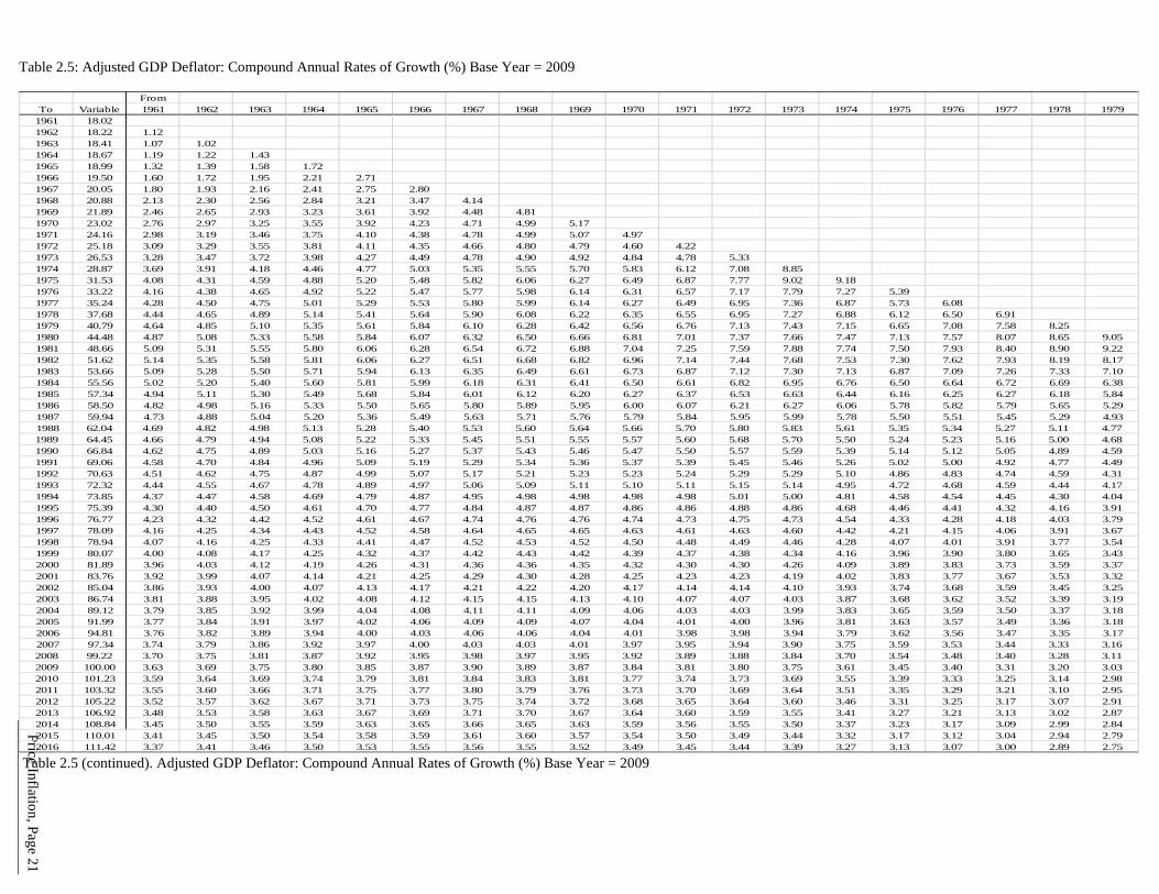
Price Inflation, Page 21
Table 2.5: Adjusted GDP Deflator: Compound Annual Rates of Growth (%) Base Year = 2009
Table 2.5 (continued). Adjusted GDP Deflator: Compound Annual Rates of Growth (%) Base Year = 2009
FromTo Variable 1961 1962 1963 1964 1965 1966 1967 1968 1969 1970 1971 1972 1973 1974 1975 1976 1977 1978 1979
1961 18.021962 18.22 1.121963 18.41 1.07 1.021964 18.67 1.19 1.22 1.431965 18.99 1.32 1.39 1.58 1.721966 19.50 1.60 1.72 1.95 2.21 2.711967 20.05 1.80 1.93 2.16 2.41 2.75 2.801968 20.88 2.13 2.30 2.56 2.84 3.21 3.47 4.141969 21.89 2.46 2.65 2.93 3.23 3.61 3.92 4.48 4.811970 23.02 2.76 2.97 3.25 3.55 3.92 4.23 4.71 4.99 5.171971 24.16 2.98 3.19 3.46 3.75 4.10 4.38 4.78 4.99 5.07 4.971972 25.18 3.09 3.29 3.55 3.81 4.11 4.35 4.66 4.80 4.79 4.60 4.221973 26.53 3.28 3.47 3.72 3.98 4.27 4.49 4.78 4.90 4.92 4.84 4.78 5.331974 28.87 3.69 3.91 4.18 4.46 4.77 5.03 5.35 5.55 5.70 5.83 6.12 7.08 8.851975 31.53 4.08 4.31 4.59 4.88 5.20 5.48 5.82 6.06 6.27 6.49 6.87 7.77 9.02 9.181976 33.22 4.16 4.38 4.65 4.92 5.22 5.47 5.77 5.98 6.14 6.31 6.57 7.17 7.79 7.27 5.391977 35.24 4.28 4.50 4.75 5.01 5.29 5.53 5.80 5.99 6.14 6.27 6.49 6.95 7.36 6.87 5.73 6.081978 37.68 4.44 4.65 4.89 5.14 5.41 5.64 5.90 6.08 6.22 6.35 6.55 6.95 7.27 6.88 6.12 6.50 6.911979 40.79 4.64 4.85 5.10 5.35 5.61 5.84 6.10 6.28 6.42 6.56 6.76 7.13 7.43 7.15 6.65 7.08 7.58 8.251980 44.48 4.87 5.08 5.33 5.58 5.84 6.07 6.32 6.50 6.66 6.81 7.01 7.37 7.66 7.47 7.13 7.57 8.07 8.65 9.051981 48.66 5.09 5.31 5.55 5.80 6.06 6.28 6.54 6.72 6.88 7.04 7.25 7.59 7.88 7.74 7.50 7.93 8.40 8.90 9.221982 51.62 5.14 5.35 5.58 5.81 6.06 6.27 6.51 6.68 6.82 6.96 7.14 7.44 7.68 7.53 7.30 7.62 7.93 8.19 8.171983 53.66 5.09 5.28 5.50 5.71 5.94 6.13 6.35 6.49 6.61 6.73 6.87 7.12 7.30 7.13 6.87 7.09 7.26 7.33 7.101984 55.56 5.02 5.20 5.40 5.60 5.81 5.99 6.18 6.31 6.41 6.50 6.61 6.82 6.95 6.76 6.50 6.64 6.72 6.69 6.381985 57.34 4.94 5.11 5.30 5.49 5.68 5.84 6.01 6.12 6.20 6.27 6.37 6.53 6.63 6.44 6.16 6.25 6.27 6.18 5.841986 58.50 4.82 4.98 5.16 5.33 5.50 5.65 5.80 5.89 5.95 6.00 6.07 6.21 6.27 6.06 5.78 5.82 5.79 5.65 5.291987 59.94 4.73 4.88 5.04 5.20 5.36 5.49 5.63 5.71 5.76 5.79 5.84 5.95 5.99 5.78 5.50 5.51 5.45 5.29 4.931988 62.04 4.69 4.82 4.98 5.13 5.28 5.40 5.53 5.60 5.64 5.66 5.70 5.80 5.83 5.61 5.35 5.34 5.27 5.11 4.771989 64.45 4.66 4.79 4.94 5.08 5.22 5.33 5.45 5.51 5.55 5.57 5.60 5.68 5.70 5.50 5.24 5.23 5.16 5.00 4.681990 66.84 4.62 4.75 4.89 5.03 5.16 5.27 5.37 5.43 5.46 5.47 5.50 5.57 5.59 5.39 5.14 5.12 5.05 4.89 4.591991 69.06 4.58 4.70 4.84 4.96 5.09 5.19 5.29 5.34 5.36 5.37 5.39 5.45 5.46 5.26 5.02 5.00 4.92 4.77 4.491992 70.63 4.51 4.62 4.75 4.87 4.99 5.07 5.17 5.21 5.23 5.23 5.24 5.29 5.29 5.10 4.86 4.83 4.74 4.59 4.311993 72.32 4.44 4.55 4.67 4.78 4.89 4.97 5.06 5.09 5.11 5.10 5.11 5.15 5.14 4.95 4.72 4.68 4.59 4.44 4.171994 73.85 4.37 4.47 4.58 4.69 4.79 4.87 4.95 4.98 4.98 4.98 4.98 5.01 5.00 4.81 4.58 4.54 4.45 4.30 4.041995 75.39 4.30 4.40 4.50 4.61 4.70 4.77 4.84 4.87 4.87 4.86 4.86 4.88 4.86 4.68 4.46 4.41 4.32 4.16 3.911996 76.77 4.23 4.32 4.42 4.52 4.61 4.67 4.74 4.76 4.76 4.74 4.73 4.75 4.73 4.54 4.33 4.28 4.18 4.03 3.791997 78.09 4.16 4.25 4.34 4.43 4.52 4.58 4.64 4.65 4.65 4.63 4.61 4.63 4.60 4.42 4.21 4.15 4.06 3.91 3.671998 78.94 4.07 4.16 4.25 4.33 4.41 4.47 4.52 4.53 4.52 4.50 4.48 4.49 4.46 4.28 4.07 4.01 3.91 3.77 3.541999 80.07 4.00 4.08 4.17 4.25 4.32 4.37 4.42 4.43 4.42 4.39 4.37 4.38 4.34 4.16 3.96 3.90 3.80 3.65 3.432000 81.89 3.96 4.03 4.12 4.19 4.26 4.31 4.36 4.36 4.35 4.32 4.30 4.30 4.26 4.09 3.89 3.83 3.73 3.59 3.372001 83.76 3.92 3.99 4.07 4.14 4.21 4.25 4.29 4.30 4.28 4.25 4.23 4.23 4.19 4.02 3.83 3.77 3.67 3.53 3.322002 85.04 3.86 3.93 4.00 4.07 4.13 4.17 4.21 4.22 4.20 4.17 4.14 4.14 4.10 3.93 3.74 3.68 3.59 3.45 3.252003 86.74 3.81 3.88 3.95 4.02 4.08 4.12 4.15 4.15 4.13 4.10 4.07 4.07 4.03 3.87 3.68 3.62 3.52 3.39 3.192004 89.12 3.79 3.85 3.92 3.99 4.04 4.08 4.11 4.11 4.09 4.06 4.03 4.03 3.99 3.83 3.65 3.59 3.50 3.37 3.182005 91.99 3.77 3.84 3.91 3.97 4.02 4.06 4.09 4.09 4.07 4.04 4.01 4.00 3.96 3.81 3.63 3.57 3.49 3.36 3.182006 94.81 3.76 3.82 3.89 3.94 4.00 4.03 4.06 4.06 4.04 4.01 3.98 3.98 3.94 3.79 3.62 3.56 3.47 3.35 3.172007 97.34 3.74 3.79 3.86 3.92 3.97 4.00 4.03 4.03 4.01 3.97 3.95 3.94 3.90 3.75 3.59 3.53 3.44 3.33 3.162008 99.22 3.70 3.75 3.81 3.87 3.92 3.95 3.98 3.97 3.95 3.92 3.89 3.88 3.84 3.70 3.54 3.48 3.40 3.28 3.112009 100.00 3.63 3.69 3.75 3.80 3.85 3.87 3.90 3.89 3.87 3.84 3.81 3.80 3.75 3.61 3.45 3.40 3.31 3.20 3.032010 101.23 3.59 3.64 3.69 3.74 3.79 3.81 3.84 3.83 3.81 3.77 3.74 3.73 3.69 3.55 3.39 3.33 3.25 3.14 2.982011 103.32 3.55 3.60 3.66 3.71 3.75 3.77 3.80 3.79 3.76 3.73 3.70 3.69 3.64 3.51 3.35 3.29 3.21 3.10 2.952012 105.22 3.52 3.57 3.62 3.67 3.71 3.73 3.75 3.74 3.72 3.68 3.65 3.64 3.60 3.46 3.31 3.25 3.17 3.07 2.912013 106.92 3.48 3.53 3.58 3.63 3.67 3.69 3.71 3.70 3.67 3.64 3.60 3.59 3.55 3.41 3.27 3.21 3.13 3.02 2.872014 108.84 3.45 3.50 3.55 3.59 3.63 3.65 3.66 3.65 3.63 3.59 3.56 3.55 3.50 3.37 3.23 3.17 3.09 2.99 2.842015 110.01 3.41 3.45 3.50 3.54 3.58 3.59 3.61 3.60 3.57 3.54 3.50 3.49 3.44 3.32 3.17 3.12 3.04 2.94 2.792016 111.42 3.37 3.41 3.46 3.50 3.53 3.55 3.56 3.55 3.52 3.49 3.45 3.44 3.39 3.27 3.13 3.07 3.00 2.89 2.75
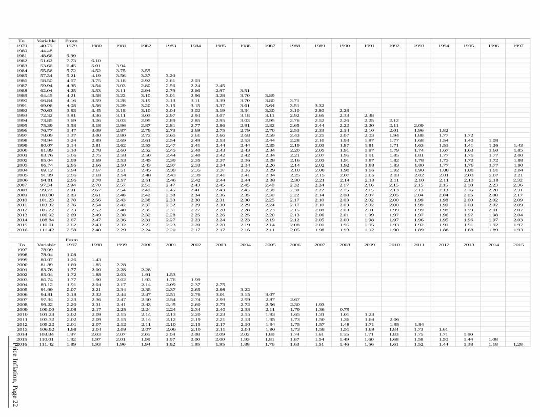
Price Inflation, Page 22
To Variable From
1979 40.79 1979 1980 1981 1982 1983 1984 1985 1986 1987 1988 1989 1990 1991 1992 1993 1994 1995 1996 19971980 44.481981 48.66 9.391982 51.62 7.73 6.101983 53.66 6.45 5.01 3.941984 55.56 5.72 4.52 3.75 3.551985 57.34 5.21 4.19 3.56 3.37 3.201986 58.50 4.67 3.75 3.18 2.92 2.61 2.031987 59.94 4.35 3.54 3.03 2.80 2.56 2.24 2.451988 62.04 4.25 3.53 3.11 2.94 2.79 2.66 2.97 3.511989 64.45 4.21 3.58 3.22 3.10 3.01 2.96 3.28 3.70 3.891990 66.84 4.16 3.59 3.28 3.19 3.13 3.11 3.39 3.70 3.80 3.711991 69.06 4.08 3.56 3.29 3.20 3.15 3.15 3.37 3.61 3.64 3.51 3.321992 70.63 3.93 3.45 3.18 3.10 3.04 3.02 3.19 3.34 3.30 3.10 2.80 2.281993 72.32 3.81 3.36 3.11 3.03 2.97 2.94 3.07 3.18 3.11 2.92 2.66 2.33 2.381994 73.85 3.69 3.26 3.03 2.95 2.89 2.85 2.95 3.03 2.95 2.76 2.52 2.26 2.25 2.121995 75.39 3.58 3.18 2.96 2.87 2.81 2.77 2.86 2.91 2.82 2.65 2.44 2.22 2.20 2.11 2.091996 76.77 3.47 3.09 2.87 2.79 2.73 2.69 2.75 2.79 2.70 2.53 2.33 2.14 2.10 2.01 1.96 1.821997 78.09 3.37 3.00 2.80 2.72 2.65 2.61 2.66 2.68 2.59 2.43 2.25 2.07 2.03 1.94 1.88 1.77 1.721998 78.94 3.24 2.89 2.69 2.61 2.54 2.49 2.53 2.53 2.44 2.28 2.10 1.93 1.87 1.77 1.68 1.54 1.40 1.081999 80.07 3.14 2.81 2.62 2.53 2.47 2.41 2.44 2.44 2.35 2.19 2.03 1.87 1.81 1.71 1.63 1.51 1.41 1.26 1.432000 81.89 3.10 2.78 2.60 2.52 2.45 2.40 2.43 2.43 2.34 2.20 2.05 1.91 1.87 1.79 1.74 1.67 1.63 1.60 1.852001 83.76 3.06 2.75 2.58 2.50 2.44 2.40 2.42 2.42 2.34 2.21 2.07 1.95 1.91 1.85 1.81 1.77 1.76 1.77 2.002002 85.04 2.99 2.69 2.53 2.45 2.39 2.35 2.37 2.36 2.28 2.16 2.03 1.91 1.87 1.82 1.78 1.73 1.72 1.72 1.882003 86.74 2.95 2.66 2.50 2.43 2.37 2.33 2.34 2.34 2.26 2.14 2.02 1.92 1.88 1.83 1.80 1.77 1.76 1.77 1.902004 89.12 2.94 2.67 2.51 2.45 2.39 2.35 2.37 2.36 2.29 2.18 2.08 1.98 1.96 1.92 1.90 1.88 1.88 1.91 2.042005 91.99 2.95 2.69 2.54 2.48 2.43 2.39 2.41 2.41 2.34 2.25 2.15 2.07 2.05 2.03 2.02 2.01 2.03 2.07 2.212006 94.81 2.95 2.70 2.57 2.51 2.46 2.42 2.44 2.44 2.38 2.30 2.21 2.14 2.13 2.11 2.10 2.11 2.13 2.18 2.322007 97.34 2.94 2.70 2.57 2.51 2.47 2.43 2.45 2.45 2.40 2.32 2.24 2.17 2.16 2.15 2.15 2.15 2.18 2.23 2.362008 99.22 2.91 2.67 2.54 2.49 2.45 2.41 2.43 2.43 2.38 2.30 2.22 2.15 2.15 2.13 2.13 2.13 2.16 2.20 2.312009 100.00 2.83 2.61 2.48 2.42 2.38 2.34 2.36 2.35 2.30 2.22 2.14 2.08 2.07 2.05 2.04 2.04 2.05 2.08 2.172010 101.23 2.78 2.56 2.43 2.38 2.33 2.30 2.31 2.30 2.25 2.17 2.10 2.03 2.02 2.00 1.99 1.98 2.00 2.02 2.092011 103.32 2.76 2.54 2.42 2.37 2.32 2.29 2.30 2.29 2.24 2.17 2.10 2.03 2.02 2.00 1.99 1.99 2.00 2.02 2.092012 105.22 2.73 2.52 2.40 2.35 2.31 2.27 2.28 2.28 2.23 2.15 2.08 2.03 2.01 1.99 1.99 1.98 1.99 2.01 2.072013 106.92 2.69 2.49 2.38 2.32 2.28 2.25 2.26 2.25 2.20 2.13 2.06 2.01 1.99 1.97 1.97 1.96 1.97 1.98 2.042014 108.84 2.67 2.47 2.36 2.31 2.27 2.23 2.24 2.23 2.19 2.12 2.05 2.00 1.98 1.97 1.96 1.95 1.96 1.97 2.032015 110.01 2.62 2.43 2.32 2.27 2.23 2.20 2.20 2.19 2.14 2.08 2.01 1.96 1.95 1.93 1.92 1.91 1.91 1.92 1.972016 111.42 2.58 2.40 2.29 2.24 2.20 2.17 2.17 2.16 2.11 2.05 1.98 1.93 1.92 1.90 1.89 1.88 1.88 1.89 1.93
FromTo Variable 1997 1998 1999 2000 2001 2002 2003 2004 2005 2006 2007 2008 2009 2010 2011 2012 2013 2014 2015
1997 78.091998 78.94 1.081999 80.07 1.26 1.432000 81.89 1.60 1.85 2.282001 83.76 1.77 2.00 2.28 2.282002 85.04 1.72 1.88 2.03 1.91 1.532003 86.74 1.77 1.90 2.02 1.93 1.76 1.992004 89.12 1.91 2.04 2.17 2.14 2.09 2.37 2.752005 91.99 2.07 2.21 2.34 2.35 2.37 2.65 2.98 3.222006 94.81 2.18 2.32 2.44 2.47 2.51 2.76 3.01 3.15 3.072007 97.34 2.23 2.36 2.47 2.50 2.54 2.74 2.93 2.99 2.87 2.672008 99.22 2.20 2.31 2.41 2.43 2.45 2.60 2.73 2.72 2.56 2.30 1.932009 100.00 2.08 2.17 2.25 2.24 2.24 2.34 2.40 2.33 2.11 1.79 1.36 0.792010 101.23 2.02 2.09 2.15 2.14 2.13 2.20 2.23 2.15 1.93 1.65 1.31 1.01 1.232011 103.32 2.02 2.09 2.15 2.14 2.12 2.19 2.21 2.13 1.95 1.73 1.50 1.36 1.64 2.062012 105.22 2.01 2.07 2.12 2.11 2.10 2.15 2.17 2.10 1.94 1.75 1.57 1.48 1.71 1.95 1.842013 106.92 1.98 2.04 2.09 2.07 2.06 2.10 2.11 2.04 1.90 1.73 1.58 1.51 1.69 1.84 1.73 1.612014 108.84 1.97 2.03 2.07 2.05 2.04 2.08 2.09 2.02 1.89 1.74 1.61 1.55 1.71 1.83 1.75 1.71 1.802015 110.01 1.92 1.97 2.01 1.99 1.97 2.00 2.00 1.93 1.81 1.67 1.54 1.49 1.60 1.68 1.58 1.50 1.44 1.082016 111.42 1.89 1.93 1.96 1.94 1.92 1.95 1.95 1.88 1.76 1.63 1.51 1.46 1.56 1.61 1.52 1.44 1.38 1.18 1.28
Price Inflation, Page 23
2.6 Appendix OCACT adjustments to the published CPI-W annual growth rates. Between 1978 and 2016, OCACT set the annual growth rate in the adjusted CPI-W to the growth rate in the published CPI-W plus an annual growth rate differential, defined as the growth rate in the CPI-U “Research Series” (CPI-U-RS) less the growth rate in the published CPI-U. BLS constructs the CPI-U-RS by recalculating the CPI-U back to 1978 using present methodology (see http://stats.bls.gov/cpi/cpiurs.htm). An exception to this specification was made because BLS introduced an improvement for “rental equivalence” in 1983 for the CPI-U, but not until 1985 for the CPI-W. Thus, for 1983 and 1984, the annual percent change in the adjusted CPI-W is defined as the percent change in the CPI-U-RS less 0.1 percentage point. This adjustment reflects the belief that, had the introductions been simultaneous in 1983, the observed differences in growth between the two inflation measures would have been equal to their published compound average annual difference (0.1 percentage point) over the post-1985 period. Between 1967 and 1977, the annual growth rate in the adjusted CPI-W was set to the growth rate in the published CPI-W less 0.2 percentage point plus an annual growth rate differential, defined as the growth rate in the CPI-U-X1 (a BLS “experimental series” that incorporates the improvement for rental equivalence into the historical CPI-U) less the growth rate in the actual published CPI-U. The 0.2 percentage point adjustment reflects a BLS estimate of the effect of introducing an improved geometric weighting formula into the CPI-W beginning in January 1999. Finally, for 1966 and earlier, the annual growth rate in the adjusted CPI-W was set to the growth rate in the published CPI-W less the 0.2 percentage point adjustment for the improved geometric formula. OCACT adjustments to the published PGDP and real GDP (and therefore productivity) annual growth rates. As mentioned above, starting in January 1999, BLS introduced a new geometric weighting formula to the CPI, estimating that it would lower the future annual growth rate in the CPI by about 0.2 percentage point. BEA estimates that this change would have had a 50.0 percent “feed-through” effect on the aggregate annual PGDP growth rate in the past. Thus, due to BLS’ introduction of an improved geometric weighting formula to the CPI, BEA lowered the annual growth rate in the aggregate PGDP by about 0.1 percentage point (0.2 * 50.0%). In addition, since the BLS improvement to the CPI does not alter the historical path of nominal GDP, BEA raised the annual real growth rate in the GDP by about 0.1 percentage point. However, BEA made these adjustments only back to 1978. Thus, to improve consistency, OCACT added the effect of this BLS improvement to the earlier data. That is, for 1978 and each earlier year, OCACT lowered the annual growth rate in the CPI by 0.2 percentage point, lowered the annual growth rate in the aggregate PGDP index by 0.1 percentage point, and raised the annual real growth rate in GDP, and therefore productivity, by 0.1 percentage point. Furthermore, a change in the CPI growth rate affects the PGDP through about 85.0% of the prices used to determine one of the components of the PGDP, that is, the GDP deflator for consumption (PGDP_C). Hence, the annual growth rate for the PGDP_C in 1978 and earlier was lowered by about 0.17 percent (0.2 * 0.85).
Average Real Wage Differential, Page 1
3. AVERAGE REAL WAGE DIFFERENTIAL
THE 2018 TRUSTEES REPORT OFFICE OF THE CHIEF ACTUARY, SOCIAL SECURITY ADMINISTRATION
TABLE OF CONTENTS PAGE
3 AVERAGE REAL WAGE DIFFERENTIAL ..................................................................... 2 3.1 SUMMARY ...................................................................................................................................................... 2 3.2 DEFINITION OF AVERAGE REAL WAGE DIFFERENTIAL ................................................................................... 2 3.3 AVERAGE REAL ECONOMY-WIDE EARNINGS GROWTH ................................................................................. 3
3.3.1 Productivity............................................................................................................................................ 5 3.3.2 Other Components: Links between Real Earnings and Productivity ..................................................... 5
3.3.2.1 Ratio of Compensation to Nominal GDP ........................................................................................................... 6 3.3.2.2 Ratio of Earnings to Compensation.................................................................................................................... 7 3.3.2.3 Average Hours Worked ...................................................................................................................................... 8 3.3.2.4 Price Differential (Expressed as Ratio of PGDP to CPI-W) ............................................................................ 10 3.3.2.5 Total Links ....................................................................................................................................................... 10
3.4 PROJECTIONS FROM OTHER SOURCES ........................................................................................................... 10 3.5 APPENDIX A ................................................................................................................................................. 13 3.6 APPENDIX B ................................................................................................................................................. 16
TABLE OF TABLES PAGE TABLE 3.1: ASSUMED AVERAGE REAL WAGE DIFFERENTIAL ........................................................................................ 2 TABLE 3.2: AVERAGE ANNUAL REAL PERCENTAGE CHANGE IN AVERAGE EARNINGS: COMPARISON OF THE U.S.
ECONOMY TO OASDI COVERED ............................................................................................................................ 4 TABLE 3.3: AVERAGE ANNUAL REAL PERCENTAGE CHANGE IN AVERAGE EARNINGS: TOTAL U.S. ECONOMY AND ITS
COMPONENTS ......................................................................................................................................................... 6 TABLE 3.4: AVERAGE HOURS WORKED PER WEEK, TOTAL U.S.: COMPOUND ANNUAL RATES OF CHANGE (%) ......... 11
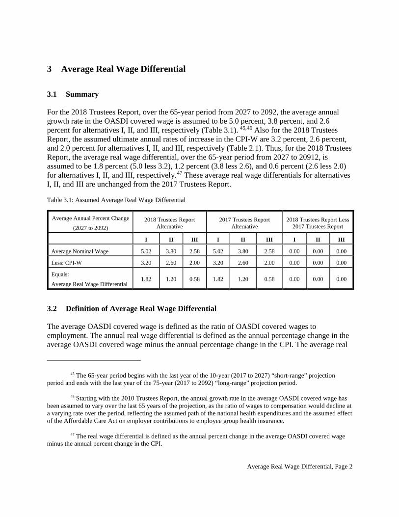
Average Real Wage Differential, Page 2
3 Average Real Wage Differential
3.1 Summary For the 2018 Trustees Report, over the 65-year period from 2027 to 2092, the average annual growth rate in the OASDI covered wage is assumed to be 5.0 percent, 3.8 percent, and 2.6 percent for alternatives I, II, and III, respectively (Table 3.1). 45,46 Also for the 2018 Trustees Report, the assumed ultimate annual rates of increase in the CPI-W are 3.2 percent, 2.6 percent, and 2.0 percent for alternatives I, II, and III, respectively (Table 2.1). Thus, for the 2018 Trustees Report, the average real wage differential, over the 65-year period from 2027 to 20912, is assumed to be 1.8 percent (5.0 less 3.2), 1.2 percent (3.8 less 2.6), and 0.6 percent (2.6 less 2.0) for alternatives I, II, and III, respectively.47 These average real wage differentials for alternatives I, II, and III are unchanged from the 2017 Trustees Report. Table 3.1: Assumed Average Real Wage Differential
Average Annual Percent Change
(2027 to 2092) 2018 Trustees Report
Alternative 2017 Trustees Report
Alternative 2018 Trustees Report Less
2017 Trustees Report
I II III I II III I II III
Average Nominal Wage 5.02 3.80 2.58 5.02 3.80 2.58 0.00 0.00 0.00
Less: CPI-W 3.20 2.60 2.00 3.20 2.60 2.00 0.00 0.00 0.00
Equals:
Average Real Wage Differential 1.82 1.20 0.58 1.82 1.20 0.58 0.00 0.00 0.00
3.2 Definition of Average Real Wage Differential The average OASDI covered wage is defined as the ratio of OASDI covered wages to employment. The annual real wage differential is defined as the annual percentage change in the average OASDI covered wage minus the annual percentage change in the CPI. The average real
45 The 65-year period begins with the last year of the 10-year (2017 to 2027) “short-range” projection period and ends with the last year of the 75-year (2017 to 2092) “long-range” projection period.
46 Starting with the 2010 Trustees Report, the annual growth rate in the average OASDI covered wage has been assumed to vary over the last 65 years of the projection, as the ratio of wages to compensation would decline at a varying rate over the period, reflecting the assumed path of the national health expenditures and the assumed effect of the Affordable Care Act on employer contributions to employee group health insurance.
47 The real wage differential is defined as the annual percent change in the average OASDI covered wage minus the annual percent change in the CPI.
Average Real Wage Differential, Page 3
wage differential over the 65-year period from 2027 to 2092 is the average of annual real wage differentials over the period. Both the income to the Social Security program and the benefits paid are related to total covered earnings (i.e., the combination of covered wages and covered net earnings from self-employment). For this reason, the growth in average earnings, not average wages, is the subject of the balance of this section. The future real growth rates in the average U.S. earnings, average U.S. wages, and the average OASDI covered wage, are expected to be approximately equal.
3.3 Average Real Economy-Wide Earnings Growth Average real earnings in the total U.S. economy are defined as the ratio of total nominal earnings (wage and salary disbursements and net proprietors’ income) to total adjusted civilian employment (see Section 3.5 Appendix A) and U.S. Armed Forces, divided by the adjusted CPI-W. BEA estimates historical values for nominal earnings as part of its broader responsibility of maintaining the NIPA for the U.S. economy. BLS estimates the CPI-W and the civilian employment from its monthly CPS data. Because CPS data for the U.S. represent average weekly employment, the growth in average earnings for the total U.S. economy represents the growth in average weekly earnings for those employed. Average real weekly earnings in the total U.S. economy increased at an average annual rate of 0.96 percent over the last 40 years (1976-2016), 1.22 percent over the last 30 years (1986-2016), 1.20 percent over the last 20 years (1996-2016), and 0.60 percent over the last 10 years (2006-2016). The average real earnings of OASDI covered workers (which differs from average real weekly earnings in the total economy partly because of changes in the number and kind of workers covered by the OASDI program) increased at an average annual rate of 0.91 percent over the last 40 years, 0.83 percent over the last 30 years, 1.58 percent over the last 20 years, and 0.71 percent over the last 10 years (see Table 3.2 below). Note that these periods do not cover complete economic cycles and thus may not be the best indicators of true trend growth rates. Federal civilian government employees will become completely covered under OASDI around 2030 (all employees hired after 1983 are covered). As a result, the composition of OASDI covered employment, which has varied since 1940, will stabilize around 2030. This suggests that it is reasonable to evaluate the 1.17 percent assumed average real rate of increase for covered earnings for alternative II in relation to the historical real growth rate in earnings for all workers in the total economy. Therefore, the balance of this section focuses on the past trends for average earnings in the U.S. economy. Considering complete economic cycles, the average annual real growth rate in earnings for all workers in the total U.S. economy was 2.08 percent from 1966 to 1973 (7 years), -0.45 percent from 1973 to 1979 (6 years), 0.47 percent from 1979 to 1989 (10 years), 2.08 percent from 1989
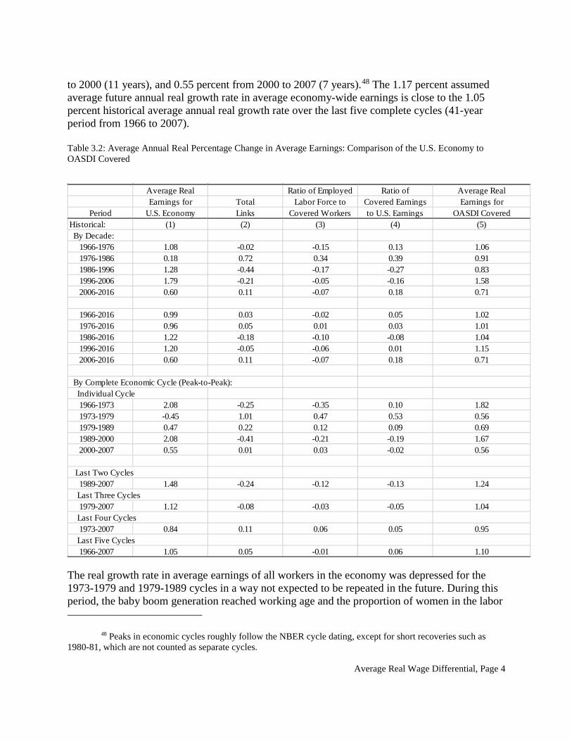
Average Real Wage Differential, Page 4
to 2000 (11 years), and 0.55 percent from 2000 to 2007 (7 years).48 The 1.17 percent assumed average future annual real growth rate in average economy-wide earnings is close to the 1.05 percent historical average annual real growth rate over the last five complete cycles (41-year period from 1966 to 2007). Table 3.2: Average Annual Real Percentage Change in Average Earnings: Comparison of the U.S. Economy to OASDI Covered
The real growth rate in average earnings of all workers in the economy was depressed for the 1973-1979 and 1979-1989 cycles in a way not expected to be repeated in the future. During this period, the baby boom generation reached working age and the proportion of women in the labor
48 Peaks in economic cycles roughly follow the NBER cycle dating, except for short recoveries such as 1980-81, which are not counted as separate cycles.
Average Real Ratio of Employed Ratio of Average RealEarnings for Total Labor Force to Covered Earnings Earnings for
Period U.S. Economy Links Covered Workers to U.S. Earnings OASDI CoveredHistorical: (1) (2) (3) (4) (5) By Decade: 1966-1976 1.08 -0.02 -0.15 0.13 1.06 1976-1986 0.18 0.72 0.34 0.39 0.91 1986-1996 1.28 -0.44 -0.17 -0.27 0.83 1996-2006 1.79 -0.21 -0.05 -0.16 1.58 2006-2016 0.60 0.11 -0.07 0.18 0.71
1966-2016 0.99 0.03 -0.02 0.05 1.02 1976-2016 0.96 0.05 0.01 0.03 1.01 1986-2016 1.22 -0.18 -0.10 -0.08 1.04 1996-2016 1.20 -0.05 -0.06 0.01 1.15 2006-2016 0.60 0.11 -0.07 0.18 0.71
By Complete Economic Cycle (Peak-to-Peak): Individual Cycle 1966-1973 2.08 -0.25 -0.35 0.10 1.82 1973-1979 -0.45 1.01 0.47 0.53 0.56 1979-1989 0.47 0.22 0.12 0.09 0.69 1989-2000 2.08 -0.41 -0.21 -0.19 1.67 2000-2007 0.55 0.01 0.03 -0.02 0.56
Last Two Cycles 1989-2007 1.48 -0.24 -0.12 -0.13 1.24 Last Three Cycles 1979-2007 1.12 -0.08 -0.03 -0.05 1.04 Last Four Cycles 1973-2007 0.84 0.11 0.06 0.05 0.95 Last Five Cycles 1966-2007 1.05 0.05 -0.01 0.06 1.10

Average Real Wage Differential, Page 5
force increased dramatically. As a result, the economy accommodated an extraordinary number of relatively low-paid (inexperienced and young) workers, thus depressing the real growth in the overall average earnings. However, the inclusion of baby boomers in the labor force ended in the mid-1980s, and the increasing percentage of women under age 60 in the labor force stabilized more recently. The rapid increase in average earnings during the complete economic cycle from 1989 to 2000 may reflect maturation of the baby boomers and women in the labor force. The large number of baby boomers and women in the labor force have been reaching prime working ages and thus boosted growth since 1989. This kind of swing in demographic trends is not projected to occur in the future, so consideration of the longer period of the last five complete economic cycles seems appropriate. This approach allows us to average out the effects of past demographic trends, which initially depressed and later boosted average earnings growth. Additional circumstances contributing to potential future growth are discussed in the next two sections on productivity growth and earnings links to productivity.
3.3.1 Productivity Total-economy productivity is defined as the ratio of real GDP to total hours worked in the U.S. economy. For the 2018 Trustees Report, the assumed ultimate annual rates of increase in total-economy productivity to 1.98 percent, 1.68 percent, and 1.38 percent for alternatives I, II, and III, respectively. These ultimate rates of increase for total-economy productivity are approximately consistent with ultimate annual rates of increase in nonfarm business productivity of 2.42 percent, 2.06 percent, and 1.69 percent for alternatives I, II, and III, respectively (see Section 1).
3.3.2 Other Components: Links between Real Earnings and Productivity Not all of the historical gains in productivity have resulted in proportional increases in average real earnings. For example, over the last four economic cycles (1973-2007), average real earnings increased at an average annual rate of only 0.84 percent per year, while productivity for the total U.S. economy increased at 1.64 percent per year. The approximate difference of -0.78 percent per year (1.0084 / 1.0164; values are rounded) was due to changes in the links, that is, those factors that connect productivity to average real earnings in a multiplicative fashion. Table 3.3 summarizes the U.S. experience over the last five decades for each of these factors.49 They include the ratio of compensation to nominal GDP, the ratio of earnings to compensation, the ratio of total hours worked to total average (weekly) employment, and the ratio of the gross
49 Section 3 calculates values for productivity, hours per week, price differential, and average real earnings using adjusted data for the CPI, PGDP, real GDP, and employment (weeks worked). Hence, Table 3.3 contains adjusted productivity values, which may not equal the unadjusted productivity values on Table 1.4 in Section 1. Adjustments to the CPI, PGDP and real GDP are described in Section 2.6 Appendix. Adjustments to employment are described in Section 3.5 Appendix A.
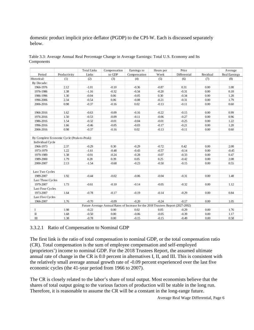
Average Real Wage Differential, Page 6
domestic product implicit price deflator (PGDP) to the CPI-W. Each is discussed separately below.
3.3.2.1 Ratio of Compensation to Nominal GDP The first link is the ratio of total compensation to nominal GDP, or the total compensation ratio (CR). Total compensation is the sum of employee compensation and self-employed (proprietors’) income to nominal GDP. For the 2018 Trustees Report, the assumed ultimate annual rate of change in the CR is 0.0 percent in alternatives I, II, and III. This is consistent with the relatively small average annual growth rate of -0.09 percent experienced over the last five economic cycles (the 41-year period from 1966 to 2007). The CR is closely related to the labor’s share of total output. Most economists believe that the shares of total output going to the various factors of production will be stable in the long run. Therefore, it is reasonable to assume the CR will be a constant in the long-range future.
Total Links Compensation Earnings to Hours per Price AveragePeriod Productivity Links to GDP Compensation Week Differential Residual Real Earnings
Historical: (1) (2) (3) (4) (5) (6) (7) (8) By Decade: 1966-1976 2.12 -1.01 -0.10 -0.36 -0.87 0.31 0.00 1.08 1976-1986 1.38 -1.16 -0.32 -0.34 -0.20 -0.31 0.00 0.18 1986-1996 1.30 -0.04 0.06 -0.05 0.30 -0.34 0.00 1.28 1996-2006 2.34 -0.54 0.06 -0.08 -0.21 -0.31 0.00 1.79 2006-2016 0.98 -0.37 -0.16 0.02 -0.13 -0.11 0.00 0.60
1966-2016 1.62 -0.63 -0.09 -0.16 -0.22 -0.15 0.00 0.99 1976-2016 1.50 -0.53 -0.09 -0.11 -0.06 -0.27 0.00 0.96 1986-2016 1.54 -0.32 -0.01 -0.04 -0.01 -0.25 0.00 1.22 1996-2016 1.66 -0.46 -0.05 -0.03 -0.17 -0.21 0.00 1.20 2006-2016 0.98 -0.37 -0.16 0.02 -0.13 -0.11 0.00 0.60
By Complete Economic Cycle (Peak-to-Peak): Individual Cycle 1966-1973 2.37 -0.29 0.30 -0.29 -0.72 0.42 0.00 2.08 1973-1979 1.22 -1.61 -0.48 -0.43 -0.57 -0.14 0.00 -0.45 1979-1989 1.38 -0.91 -0.24 -0.28 -0.07 -0.33 0.00 0.47 1989-2000 1.79 0.28 0.39 0.05 0.25 -0.42 0.00 2.08 2000-2007 2.13 -1.54 -0.68 -0.23 -0.50 -0.15 0.00 0.55
Last Two Cycles 1989-2007 1.92 -0.44 -0.02 -0.06 -0.04 -0.31 0.00 1.48 Last Three Cycles 1979-2007 1.73 -0.61 -0.10 -0.14 -0.05 -0.32 0.00 1.12 Last Four Cycles 1973-2007 1.64 -0.78 -0.17 -0.19 -0.14 -0.29 0.00 0.84 Last Five Cycles 1966-2007 1.76 -0.70 -0.09 -0.20 -0.24 -0.17 0.00 1.05
I 1.98 -0.22 0.00 0.02 0.05 -0.29 0.00 1.76 II 1.68 -0.50 0.00 -0.06 -0.05 -0.39 0.00 1.17 III 1.38 -0.78 0.00 -0.15 -0.15 -0.49 0.00 0.58
Future Average Annual Rates of Increase for the 2018 Trustees Report (2027-2092)
Table 3.3: Average Annual Real Percentage Change in Average Earnings: Total U.S. Economy and Its Components

Average Real Wage Differential, Page 7
3.3.2.2 Ratio of Earnings to Compensation The second link is the ratio of total worker earnings to compensation. Using NIPA definitions, total worker earnings are the sum of total wage and salary disbursements and total proprietors’ income. Total compensation is the sum of employee compensation and total proprietors’ income. Total employee compensation is the sum of total wage and salary disbursements, employer contributions for employee pension and insurance funds, and employer contributions to government social insurance. Employer contributions to government social insurance include payments for public insurance and publicly mandated insurance such as for unemployment, workers’ compensation, Medicare, and Social Security. The average annual rate of change for the ratio was -0.20 percent from 1966 to 2007, a 41-year period that covers the last five peak-to-peak economic cycles. The historical decline in the ratio has been due primarily to the relatively faster growth in employer contributions to employee pensions and health insurance. Most employer contributions to pensions are for employees in the private sector and are composed of contributions to defined-benefit (DB) and defined-contribution (DC) plans. After declining in the 1980s and 1990s, when the work force was relatively young, asset returns relatively high, and the proportion of employees covered by DB plans was beginning to decline, employer contributions to pension plans rose sharply between 1997 and 2010 as the workforce aged, the stock market experienced two major crashes, and interest rates reached unusually low levels. Counteracting these recent trends is the continuing decline in DB coverage. The contributions have declined somewhat since 2010 as the stock market rebounded and may decline further in the near future if interest rates rise from current low levels. OCACT also expects a relative increase in employer contributions to employee pension funds due to increased life expectancy, and a relative decrease due to a continued shift from defined-benefit to defined-contribution plans. Contributions to employer-sponsored group health insurance (ESI) in the future are expected to be significantly affected by the Affordable Care Act enacted in 2010. This expectation led to a significant change in the assumed future path of the ratio of earnings to compensation between the 2009 and subsequent Trustees Reports.50 For the 2018 Trustees Report, the annual rates of change in the ratio of WSD to WSS are assumed to be consistent with CMS’s most recent projections of ESI. In September 2017, CMS revised its projections of ESI for the period 2020-91. The revised CMS projections differ little from the 2016 projections. The assumed path for the annual rates of change in the ratio of WSD to WSS over the last 65 years of the projection horizon (2027 to 2092) is consistent with the annual rates of change from the revised CMS projections and the National Health Expenditure projections for 2016-25 released in March 2017.51 This will result in an average annual rate of growth in the ratio of WSD to WSS of about -0.08 percent for alternative II over the last 65 years of the 75-year projection period.
50 For details, see Section 3.6 Appendix B. 51 https://www.cms.gov/Research-Statistics-Data-and-Systems/Statistics-Trends-and-
Reports/NationalHealthExpendData/Downloads/proj2016.pdf
Average Real Wage Differential, Page 8
Hence, for the 2018 Trustees Report, the average annual rate of change in the ratio of wages to employee compensation over the last 65 years of the projection horizon (2027 to 2092) is assumed to be 0.02, -0.08, and -0.18 percentage point for alternatives I, II, and III, respectively. Consistent with this, the assumed average annual rate of change in the ratio of earnings to total compensation over the last 65 years of the projection horizon (2027 to 2092) is 0.02, -0.06, and -0.15 percentage point for alternatives I, II, and III, respectively.
3.3.2.3 Average Hours Worked The third link is average hours worked per week (AHW), defined as the ratio of total hours worked to total employment in the U.S. economy. Its compounded annual rate of change is shown in Table 3.4. Total hours worked in the U.S. economy is a special request series provided by BLS, based mostly on the CES. Total employment, computed on an average weekly basis, is the sum of civilian employment and the U.S. Armed Forces. BLS publishes total civilian employment from the CPS. The Census Bureau provides estimates for the U.S. Armed Forces. For the 2018 Trustees Report, the assumed ultimate annual rate of change in average hours worked is +0.05 percent, -0.05 percent and -0.15 percent in alternatives I, II, and III, respectively. These rates of change are the same as those used in the 2017 Trustees Report. The average annual rate of change in AHW was -0.24 percent over the last five economic cycles, a 41-year period from 1966 to 2007. Looking at individual cycles, the average annual rate of change in AHW was -0.72 percent, -0.57 percent, -0.07 percent, 0.25 percent, and -0.50 percent, over the 1966-1973, 1973-1979, 1979-1989, 1989-2000, and 2000-2007 periods, respectively. To reflect, in part, the shift from negative to positive rates of change over the 1966 to 2000 period, the Trustees raised the assumed ultimate intermediate case annual rate of change in AHW from -0.2 percent for the 1996 Trustees Report to -0.1 percent for the 1997 through 2002 Reports, and to 0.0 percent for the 2003 through 2011 Reports. Some of the reversal in the historical decline in AHW between 1982 and 1999 is due to changes in the education and age-sex distributions of the workforce. Workers with higher education tend to work more hours than their less-educated counterparts, males tend to work more hours than females, and prime-age workers more than the very young and the very old. In analyses for the 2001 Trustees Reports (see memorandum dated October 6, 2000 on AHW for more details), OCACT estimated that, due to changes in the education and age-sex distributions of the workforce alone, the average annual rate of change in AHW increased by about 0.18 percent per year over the 1979-1989 period, and by 0.06 percent over the 1989-1998 period. Thus, as a rough approximation, the underlying “trend” rate of change in the AHW was estimated to be about -0.25 percent (-0.07 − 0.18) over the 1979-1989 economic cycle, and about 0.19 percent (0.25 − 0.06) over the 1989-2000 economic cycle. The historical pattern of AHW, as defined in this section, is also affected by the difference between CES and CPS employment measures. While CES estimates the number of jobs in the economy, CPS estimates the number of employed persons. Furthermore, CPS estimates are controlled to population annually between censuses. This causes the ratio of the two measures to
Average Real Wage Differential, Page 9
change over time. Since 2015, BLS has made both the total hours worked and the employment estimate on which it is based available as a special request file.52 The ratio between the employment measure implicit in the BLS measure of total hours worked and the total employment measure used in this section (i.e., CPS-based civilian employment plus the Census estimate of armed forces) has fluctuated between about 1.03 and 1.07. Notably, it was rising steadily in the last decade of the 20th century and declining in the first decade of the 21st century. The average annual rate of change in the average weekly hours implicit in the BLS calculation of total hours worked was -0.62 percent, -0.50 percent, -0.01 percent, -0.03 percent, and -0.25 percent, over the 1966-1973, 1973-1979, 1979-1989, 1989-2000, and 2000-2007 periods, respectively. The average annual rate of change over the last five economic cycles (1966 to 2007) was -0.23 percent, which is almost equal to the average rate of change calculated using the CPS-based employment measure.53 Other data from the CPS also suggested that the trend movement in the average annual rate of change in AHW was close to 0.0 percent over the 1989 to 2000 period. BLS publishes a CPS-based measure of average hours worked per week for the total labor force (AHW_CPS). The average annual rate of change in the AHW_CPS was about 0.02 percent over the 1989 to 2000 period. If the effect of changes in the education and age-sex distributions of the workforce is removed from this measure, the residual average annual rate of change in the AHW_CPS would have been about -0.04 percent (0.02 − 0.06) over the period. The average annual rate of change in AHW was -0.50 percent over the last economic cycle, a 7-year period from 2000 to 2007, suggesting a return to the steep declines over the period from 1966 to 1979. However, the magnitude of this drop may be due to differences in employment estimates described above, as the average annual rate of change implicit in the BLS estimates of total hours worked is -0.25 percent. Also, the average annual rate of change in AHW_CPS was about 0.22 percent over the period, again suggesting a more moderate decline. Regardless, the return to declines in the rate of change in AHW since 2000 was substantial. Accordingly, the Trustees lowered the assumed ultimate annual rate of change in AHW to -0.05 percent starting with the 2012 Report, or approximately equal to the average annual rate of change of -0.05 percent over the last three economic cycles, a 28-year period from 1979 to 2007.54 There are factors that may affect the future AHW in offsetting ways. On one hand, the assumed steady increases in productivity will allow workers to gradually increase leisure time while still maintaining increases in weekly and annual earnings. On the other hand, it is reasonable to assume that the assumed future increases in life expectancy will raise labor force participation rates for older workers and it may also raise AHW, holding other factors constant. The average
52 http://www.bls.gov/lpc/special_requests/us_total_hrs_emp.xlsx. 53 One could further decouple the “average hours worked” link into two links, roughly corresponding to
average hours per job and average jobs per worker. However, despite fluctuations over economic cycles and between censuses, the latter link seems to be very stable over longer time periods, so that such an additional step seems unnecessary for the purpose of deriving assumptions about the future.
54 The corresponding value implicit in the BLS estimate of total hours worked is -0.08 percent.
Average Real Wage Differential, Page 10
projected changes in the education and age-sex distributions of the workforce are not expected to significantly affect the average annual rate of change in the AHW in the future.
3.3.2.4 Price Differential (Expressed as Ratio of PGDP to CPI-W) The final link is the ratio of the PGDP to the CPI-W. Including this ratio is necessary because nominal earnings depend on nominal GDP (i.e., the product of real GDP and the PGDP), but are converted to real earnings using the CPI-W. For the 2018 Trustees Report, the assumed ultimate price differential (expressed as the PGDP less CPI-W average annual rates of increase) is -0.3, -0.4, and -0.5 percentage point for alternative I, II, and III, respectively. For alternative II, the 0.4 percentage point price differential is the sum of a 0.3 percentage point computational difference and a 0.1 percentage point coverage difference (see Section 2.3). These assumed values are unchanged from the ones assumed in the 2017 Trustees Report.
3.3.2.5 Total Links The average annual change in the total links was -0.61 percent over the last three economic cycles and -0.78 percent over the last four cycles. For the 2018 Trustees Report, the assumed average annual changes in the total links are approximately -0.22 percentage point, -0.51 percentage point, and -0.79 percentage point for alternatives I, II, and III, respectively.
3.4 Projections from Other Sources IHS Markit (formerly Global Insight, Inc.) provides projections through 2047 in its latest long-run trend forecast (see The 30-Year Focus, Third Quarter, August 2017). IHS Markit projects that the average annual real growth rate for average U.S. earnings be 1.27 percent over the 20-year period from 2027 to 2047. Moody’s Analytics’ September 2017 forecast extends to 2047. Over the 20-year period from 2027 to 2047, Moody’s Analytics projects that the annual real growth rate for average U.S. earnings will average 1.2 percent. The Office of Management and Budget (OMB) Mid-Session Review of the Fiscal Year 2018 Budget includes projections through 2027. OMB projects that the annual growth real rate for average U.S. earnings will be about 2.1 percent for 2027. The Congressional Budget Office (CBO) March 2017 report, The 2017 Long-Term Budget Outlook, includes projections through 2047. CBO projects that the annual real growth rate for average U.S. wages will average about 1.1 percent over the period 2027 to 2047. The Social Security Advisory Board’s 2015 Technical Panel on Assumptions and Methods recommended no changes to the assumed ultimate (i.e., long-range average) annual real rate of increase in the average wage of 1.17 percent in the 2015 Trustees Report, alternative II. The Technical Panel on Assumptions and Methods also endorsed OCACT’s approach to estimating the effect of health insurance cost on wages.
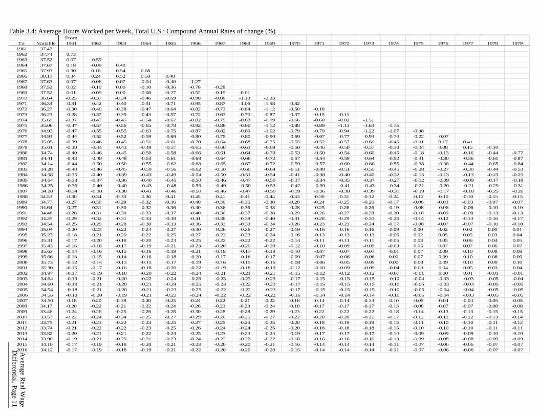
Average R
eal Wage
Differential, Page 11
Table 3.4: Average Hours Worked per Week, Total U.S.: Compound Annual Rates of change (%)
FromTo Variable 1961 1962 1963 1964 1965 1966 1967 1968 1969 1970 1971 1972 1973 1974 1975 1976 1977 1978 1979
1961 37.471962 37.74 0.731963 37.52 0.07 -0.591964 37.67 0.18 -0.09 0.401965 37.93 0.30 0.16 0.54 0.681966 38.11 0.34 0.24 0.52 0.58 0.481967 37.63 0.07 -0.06 0.07 -0.04 -0.40 -1.271968 37.52 0.02 -0.10 0.00 -0.10 -0.36 -0.78 -0.281969 37.52 0.01 -0.09 0.00 -0.08 -0.27 -0.52 -0.15 -0.011970 36.64 -0.25 -0.37 -0.34 -0.46 -0.69 -0.98 -0.88 -1.18 -2.331971 36.34 -0.31 -0.42 -0.40 -0.51 -0.71 -0.95 -0.87 -1.06 -1.58 -0.821972 36.27 -0.30 -0.40 -0.38 -0.47 -0.64 -0.82 -0.73 -0.84 -1.12 -0.50 -0.181973 36.23 -0.28 -0.37 -0.35 -0.43 -0.57 -0.72 -0.63 -0.70 -0.87 -0.37 -0.15 -0.111974 35.69 -0.37 -0.47 -0.45 -0.54 -0.67 -0.82 -0.75 -0.83 -0.99 -0.66 -0.60 -0.81 -1.511975 35.06 -0.47 -0.57 -0.56 -0.65 -0.78 -0.92 -0.88 -0.96 -1.12 -0.88 -0.89 -1.13 -1.63 -1.751976 34.93 -0.47 -0.55 -0.55 -0.63 -0.75 -0.87 -0.82 -0.89 -1.02 -0.79 -0.79 -0.94 -1.22 -1.07 -0.381977 34.91 -0.44 -0.52 -0.52 -0.59 -0.69 -0.80 -0.75 -0.80 -0.90 -0.69 -0.67 -0.77 -0.93 -0.74 -0.22 -0.071978 35.05 -0.39 -0.46 -0.45 -0.51 -0.61 -0.70 -0.64 -0.68 -0.75 -0.55 -0.52 -0.57 -0.66 -0.45 -0.01 0.17 0.411979 35.01 -0.38 -0.44 -0.43 -0.49 -0.57 -0.65 -0.60 -0.63 -0.69 -0.50 -0.46 -0.50 -0.57 -0.38 -0.04 0.08 0.15 -0.101980 34.74 -0.40 -0.46 -0.45 -0.50 -0.58 -0.66 -0.61 -0.64 -0.70 -0.53 -0.50 -0.54 -0.60 -0.45 -0.18 -0.13 -0.16 -0.44 -0.771981 34.41 -0.43 -0.49 -0.48 -0.53 -0.61 -0.68 -0.64 -0.66 -0.72 -0.57 -0.54 -0.58 -0.64 -0.52 -0.31 -0.30 -0.36 -0.61 -0.871982 34.14 -0.44 -0.50 -0.50 -0.55 -0.62 -0.68 -0.65 -0.67 -0.72 -0.59 -0.57 -0.60 -0.66 -0.55 -0.38 -0.38 -0.44 -0.65 -0.841983 34.28 -0.40 -0.46 -0.45 -0.50 -0.56 -0.62 -0.58 -0.60 -0.64 -0.51 -0.48 -0.51 -0.55 -0.45 -0.28 -0.27 -0.30 -0.44 -0.531984 34.58 -0.35 -0.40 -0.39 -0.43 -0.49 -0.54 -0.50 -0.51 -0.54 -0.41 -0.38 -0.40 -0.42 -0.32 -0.15 -0.13 -0.13 -0.23 -0.251985 34.64 -0.33 -0.37 -0.36 -0.40 -0.45 -0.50 -0.46 -0.47 -0.50 -0.37 -0.34 -0.35 -0.37 -0.27 -0.12 -0.09 -0.09 -0.17 -0.181986 34.25 -0.36 -0.40 -0.40 -0.43 -0.48 -0.53 -0.49 -0.50 -0.53 -0.42 -0.39 -0.41 -0.43 -0.34 -0.21 -0.20 -0.21 -0.29 -0.311987 34.28 -0.34 -0.38 -0.38 -0.41 -0.46 -0.50 -0.46 -0.47 -0.50 -0.39 -0.36 -0.38 -0.39 -0.31 -0.19 -0.17 -0.18 -0.25 -0.261988 34.53 -0.30 -0.34 -0.33 -0.36 -0.41 -0.45 -0.41 -0.41 -0.44 -0.33 -0.30 -0.31 -0.32 -0.24 -0.12 -0.10 -0.10 -0.15 -0.151989 34.77 -0.27 -0.30 -0.29 -0.32 -0.36 -0.40 -0.36 -0.36 -0.38 -0.28 -0.24 -0.25 -0.26 -0.17 -0.06 -0.03 -0.03 -0.07 -0.071990 34.64 -0.27 -0.31 -0.30 -0.32 -0.36 -0.40 -0.36 -0.36 -0.38 -0.28 -0.25 -0.26 -0.26 -0.19 -0.08 -0.06 -0.06 -0.10 -0.101991 34.48 -0.28 -0.31 -0.30 -0.33 -0.37 -0.40 -0.36 -0.37 -0.38 -0.29 -0.26 -0.27 -0.28 -0.20 -0.10 -0.09 -0.09 -0.13 -0.131992 34.25 -0.29 -0.32 -0.31 -0.34 -0.38 -0.41 -0.38 -0.38 -0.40 -0.31 -0.28 -0.29 -0.30 -0.23 -0.14 -0.12 -0.13 -0.16 -0.171993 34.54 -0.25 -0.29 -0.28 -0.30 -0.33 -0.36 -0.33 -0.33 -0.34 -0.26 -0.23 -0.23 -0.24 -0.17 -0.08 -0.07 -0.07 -0.10 -0.101994 35.04 -0.20 -0.23 -0.22 -0.24 -0.27 -0.30 -0.26 -0.26 -0.27 -0.19 -0.16 -0.16 -0.16 -0.09 0.00 0.02 0.02 0.00 0.011995 35.23 -0.18 -0.21 -0.20 -0.22 -0.25 -0.27 -0.23 -0.23 -0.24 -0.16 -0.13 -0.13 -0.13 -0.06 0.02 0.05 0.05 0.03 0.041996 35.31 -0.17 -0.20 -0.18 -0.20 -0.23 -0.25 -0.22 -0.22 -0.22 -0.14 -0.11 -0.11 -0.11 -0.05 0.03 0.05 0.06 0.04 0.051997 35.43 -0.16 -0.18 -0.17 -0.19 -0.21 -0.23 -0.20 -0.20 -0.20 -0.12 -0.10 -0.09 -0.09 -0.03 0.05 0.07 0.07 0.06 0.071998 35.63 -0.14 -0.16 -0.15 -0.16 -0.19 -0.21 -0.18 -0.17 -0.18 -0.10 -0.07 -0.07 -0.07 -0.01 0.07 0.09 0.10 0.08 0.091999 35.66 -0.13 -0.15 -0.14 -0.16 -0.18 -0.20 -0.17 -0.16 -0.17 -0.09 -0.07 -0.06 -0.06 0.00 0.07 0.09 0.10 0.08 0.092000 35.73 -0.12 -0.14 -0.13 -0.15 -0.17 -0.19 -0.16 -0.15 -0.16 -0.08 -0.06 -0.05 -0.05 0.00 0.08 0.09 0.10 0.09 0.102001 35.30 -0.15 -0.17 -0.16 -0.18 -0.20 -0.22 -0.19 -0.18 -0.19 -0.12 -0.10 -0.09 -0.09 -0.04 0.03 0.04 0.05 0.03 0.042002 34.97 -0.17 -0.19 -0.18 -0.20 -0.22 -0.24 -0.21 -0.21 -0.21 -0.15 -0.12 -0.12 -0.12 -0.07 -0.01 0.00 0.01 -0.01 -0.012003 34.64 -0.19 -0.21 -0.20 -0.22 -0.24 -0.26 -0.23 -0.23 -0.23 -0.17 -0.15 -0.15 -0.15 -0.10 -0.04 -0.03 -0.03 -0.05 -0.042004 34.60 -0.19 -0.21 -0.20 -0.21 -0.24 -0.25 -0.23 -0.22 -0.23 -0.17 -0.15 -0.15 -0.15 -0.10 -0.05 -0.03 -0.03 -0.05 -0.052005 34.54 -0.18 -0.21 -0.20 -0.21 -0.23 -0.25 -0.22 -0.22 -0.23 -0.17 -0.15 -0.15 -0.15 -0.10 -0.05 -0.04 -0.04 -0.05 -0.052006 34.56 -0.18 -0.20 -0.19 -0.21 -0.23 -0.24 -0.22 -0.22 -0.22 -0.16 -0.14 -0.14 -0.14 -0.10 -0.05 -0.04 -0.03 -0.05 -0.052007 34.50 -0.18 -0.20 -0.19 -0.20 -0.23 -0.24 -0.22 -0.21 -0.22 -0.16 -0.14 -0.14 -0.14 -0.10 -0.05 -0.04 -0.04 -0.05 -0.052008 34.17 -0.20 -0.22 -0.21 -0.22 -0.24 -0.26 -0.23 -0.23 -0.24 -0.18 -0.17 -0.17 -0.17 -0.13 -0.08 -0.07 -0.07 -0.08 -0.082009 33.46 -0.24 -0.26 -0.25 -0.26 -0.28 -0.30 -0.28 -0.28 -0.29 -0.23 -0.22 -0.22 -0.22 -0.18 -0.14 -0.13 -0.13 -0.15 -0.152010 33.57 -0.22 -0.24 -0.24 -0.25 -0.27 -0.29 -0.26 -0.26 -0.27 -0.22 -0.20 -0.20 -0.21 -0.17 -0.12 -0.12 -0.12 -0.13 -0.142011 33.75 -0.21 -0.23 -0.22 -0.23 -0.25 -0.27 -0.25 -0.25 -0.25 -0.20 -0.18 -0.19 -0.19 -0.15 -0.11 -0.10 -0.10 -0.11 -0.122012 33.74 -0.21 -0.22 -0.22 -0.23 -0.25 -0.26 -0.24 -0.24 -0.25 -0.20 -0.18 -0.18 -0.18 -0.15 -0.10 -0.10 -0.10 -0.11 -0.112013 33.82 -0.20 -0.21 -0.21 -0.22 -0.24 -0.25 -0.23 -0.23 -0.24 -0.19 -0.17 -0.17 -0.17 -0.14 -0.09 -0.09 -0.09 -0.10 -0.102014 33.90 -0.19 -0.21 -0.20 -0.21 -0.23 -0.24 -0.22 -0.22 -0.22 -0.18 -0.16 -0.16 -0.16 -0.13 -0.09 -0.08 -0.08 -0.09 -0.092015 34.10 -0.17 -0.19 -0.18 -0.20 -0.21 -0.23 -0.20 -0.20 -0.21 -0.16 -0.14 -0.14 -0.14 -0.11 -0.07 -0.06 -0.06 -0.07 -0.072016 34.12 -0.17 -0.19 -0.18 -0.19 -0.21 -0.22 -0.20 -0.20 -0.20 -0.15 -0.14 -0.14 -0.14 -0.11 -0.07 -0.06 -0.06 -0.07 -0.07
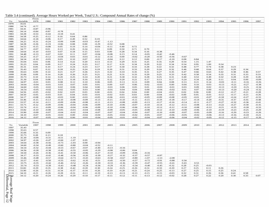
Average R
eal Wage
Differential, Page 12
Table 3.4 (continued). Average Hours Worked per Week, Total U.S.: Compound Annual Rates of change (%)
FromTo Variable 1979 1980 1981 1982 1983 1984 1985 1986 1987 1988 1989 1990 1991 1992 1993 1994 1995 1996 1997
1979 35.011980 34.74 -0.771981 34.41 -0.87 -0.961982 34.14 -0.84 -0.87 -0.781983 34.28 -0.53 -0.44 -0.18 0.411984 34.58 -0.25 -0.12 0.16 0.64 0.861985 34.64 -0.18 -0.06 0.17 0.49 0.52 0.191986 34.25 -0.31 -0.24 -0.09 0.08 -0.03 -0.47 -1.131987 34.28 -0.26 -0.19 -0.06 0.08 0.00 -0.29 -0.52 0.081988 34.53 -0.15 -0.08 0.05 0.19 0.14 -0.04 -0.11 0.40 0.721989 34.77 -0.07 0.01 0.13 0.26 0.24 0.11 0.09 0.50 0.71 0.701990 34.64 -0.10 -0.03 0.07 0.18 0.15 0.03 0.00 0.28 0.34 0.16 -0.381991 34.48 -0.13 -0.07 0.02 0.11 0.07 -0.04 -0.08 0.13 0.14 -0.05 -0.42 -0.461992 34.25 -0.17 -0.12 -0.04 0.03 -0.01 -0.12 -0.16 0.00 -0.02 -0.20 -0.50 -0.56 -0.671993 34.54 -0.10 -0.05 0.03 0.10 0.07 -0.01 -0.04 0.12 0.12 0.00 -0.17 -0.10 0.08 0.841994 35.04 0.01 0.06 0.14 0.22 0.20 0.13 0.13 0.29 0.31 0.25 0.16 0.29 0.54 1.15 1.471995 35.23 0.04 0.09 0.17 0.24 0.23 0.17 0.17 0.31 0.34 0.29 0.22 0.34 0.54 0.95 1.00 0.541996 35.31 0.05 0.10 0.17 0.24 0.23 0.17 0.17 0.30 0.33 0.28 0.22 0.32 0.48 0.77 0.74 0.38 0.231997 35.43 0.07 0.12 0.18 0.25 0.24 0.19 0.19 0.31 0.33 0.29 0.24 0.32 0.46 0.68 0.64 0.37 0.29 0.341998 35.63 0.09 0.14 0.21 0.27 0.26 0.21 0.22 0.33 0.35 0.31 0.27 0.35 0.47 0.66 0.63 0.42 0.38 0.46 0.571999 35.66 0.09 0.14 0.20 0.26 0.25 0.21 0.21 0.31 0.33 0.29 0.25 0.33 0.42 0.58 0.54 0.35 0.31 0.33 0.332000 35.73 0.10 0.14 0.20 0.25 0.24 0.20 0.21 0.30 0.32 0.28 0.25 0.31 0.40 0.53 0.49 0.32 0.28 0.29 0.282001 35.30 0.04 0.08 0.13 0.18 0.16 0.12 0.12 0.20 0.21 0.17 0.13 0.17 0.24 0.34 0.28 0.11 0.04 0.00 -0.092002 34.97 -0.01 0.03 0.08 0.12 0.10 0.06 0.05 0.13 0.13 0.09 0.04 0.08 0.13 0.21 0.14 -0.03 -0.11 -0.16 -0.262003 34.64 -0.04 -0.01 0.03 0.07 0.05 0.01 0.00 0.07 0.06 0.02 -0.03 0.00 0.04 0.10 0.03 -0.13 -0.21 -0.27 -0.382004 34.60 -0.05 -0.02 0.02 0.06 0.04 0.00 -0.01 0.06 0.05 0.01 -0.03 -0.01 0.03 0.09 0.02 -0.13 -0.20 -0.25 -0.342005 34.54 -0.05 -0.02 0.02 0.05 0.03 0.00 -0.01 0.04 0.04 0.00 -0.04 -0.02 0.01 0.07 0.00 -0.13 -0.20 -0.24 -0.322006 34.56 -0.05 -0.02 0.02 0.05 0.03 0.00 -0.01 0.04 0.04 0.00 -0.04 -0.01 0.02 0.06 0.00 -0.12 -0.17 -0.21 -0.282007 34.50 -0.05 -0.03 0.01 0.04 0.03 -0.01 -0.02 0.03 0.03 0.00 -0.04 -0.02 0.00 0.05 -0.01 -0.12 -0.17 -0.21 -0.262008 34.17 -0.08 -0.06 -0.03 0.00 -0.01 -0.05 -0.06 -0.01 -0.02 -0.05 -0.09 -0.08 -0.05 -0.01 -0.07 -0.18 -0.24 -0.27 -0.332009 33.46 -0.15 -0.13 -0.10 -0.08 -0.09 -0.13 -0.15 -0.10 -0.11 -0.15 -0.19 -0.18 -0.17 -0.14 -0.20 -0.31 -0.37 -0.41 -0.482010 33.57 -0.14 -0.11 -0.09 -0.06 -0.08 -0.11 -0.13 -0.08 -0.09 -0.13 -0.17 -0.16 -0.14 -0.11 -0.17 -0.27 -0.32 -0.36 -0.412011 33.75 -0.12 -0.09 -0.06 -0.04 -0.06 -0.09 -0.10 -0.06 -0.07 -0.10 -0.14 -0.12 -0.11 -0.08 -0.13 -0.22 -0.27 -0.30 -0.352012 33.74 -0.11 -0.09 -0.06 -0.04 -0.06 -0.09 -0.10 -0.06 -0.06 -0.10 -0.13 -0.12 -0.10 -0.08 -0.12 -0.21 -0.25 -0.28 -0.332013 33.82 -0.10 -0.08 -0.05 -0.03 -0.04 -0.08 -0.09 -0.05 -0.05 -0.08 -0.12 -0.10 -0.09 -0.06 -0.10 -0.19 -0.23 -0.25 -0.292014 33.90 -0.09 -0.07 -0.04 -0.02 -0.04 -0.07 -0.07 -0.04 -0.04 -0.07 -0.10 -0.09 -0.07 -0.05 -0.09 -0.16 -0.20 -0.23 -0.262015 34.10 -0.07 -0.05 -0.03 0.00 -0.02 -0.04 -0.05 -0.02 -0.02 -0.05 -0.07 -0.06 -0.05 -0.02 -0.06 -0.13 -0.16 -0.18 -0.212016 34.12 -0.07 -0.05 -0.02 0.00 -0.01 -0.04 -0.05 -0.01 -0.02 -0.04 -0.07 -0.06 -0.04 -0.02 -0.05 -0.12 -0.15 -0.17 -0.20
FromTo Variable 1997 1998 1999 2000 2001 2002 2003 2004 2005 2006 2007 2008 2009 2010 2011 2012 2013 2014 2015
1997 35.431998 35.63 0.571999 35.66 0.33 0.092000 35.73 0.28 0.13 0.182001 35.30 -0.09 -0.31 -0.51 -1.192002 34.97 -0.26 -0.47 -0.66 -1.07 0.952003 34.64 -0.38 -0.56 -0.73 -1.03 0.00 -0.942004 34.60 -0.34 -0.49 -0.60 -0.80 -0.04 -0.52 -0.112005 34.54 -0.32 -0.44 -0.53 -0.67 -0.07 -0.40 -0.13 -0.162006 34.56 -0.28 -0.38 -0.45 -0.55 -0.05 -0.29 -0.08 -0.06 0.042007 34.50 -0.26 -0.36 -0.41 -0.50 -0.06 -0.27 -0.10 -0.09 -0.06 -0.162008 34.17 -0.33 -0.42 -0.48 -0.56 -0.20 -0.39 -0.27 -0.32 -0.37 -0.57 -0.972009 33.46 -0.48 -0.57 -0.64 -0.73 -0.43 -0.63 -0.58 -0.67 -0.80 -1.07 -1.53 -2.082010 33.57 -0.41 -0.50 -0.55 -0.62 -0.35 -0.51 -0.45 -0.50 -0.57 -0.72 -0.91 -0.88 0.342011 33.75 -0.35 -0.42 -0.46 -0.52 -0.26 -0.39 -0.33 -0.36 -0.39 -0.47 -0.55 -0.41 0.43 0.532012 33.74 -0.33 -0.39 -0.43 -0.48 -0.24 -0.36 -0.29 -0.32 -0.34 -0.40 -0.45 -0.32 0.28 0.25 -0.032013 33.82 -0.29 -0.35 -0.38 -0.42 -0.20 -0.30 -0.24 -0.25 -0.26 -0.31 -0.33 -0.20 0.27 0.25 0.11 0.262014 33.90 -0.26 -0.31 -0.34 -0.37 -0.16 -0.26 -0.19 -0.20 -0.21 -0.24 -0.25 -0.13 0.27 0.25 0.15 0.25 0.242015 34.10 -0.21 -0.26 -0.28 -0.31 -0.11 -0.19 -0.13 -0.13 -0.13 -0.15 -0.15 -0.03 0.32 0.31 0.26 0.36 0.41 0.582016 34.12 -0.20 -0.24 -0.26 -0.29 -0.10 -0.17 -0.11 -0.12 -0.11 -0.13 -0.12 -0.02 0.28 0.27 0.22 0.29 0.30 0.33 0.07
Average Real Wage Differential, Page 13
3.5 Appendix A BLS has introduced numerous changes to the Current Population Survey (CPS) concepts over the historical period, such that values for employment are not historically comparable over the period (for more detail on noncomparability of CPS concepts, see http://www.bls.gov/cps/eetech_methods.pdf). To make the total employment series more comparable, OCACT adjusted the published values for the following: 1990 Census − 1990 Census-based population controls were introduced in January 1994 by BLS, increasing employment levels for 1990 from the originally-published estimates by about 880,000 (0.7%). BLS later revised the 1990 to 1993 estimates, but not those for earlier years. Consequently, OCACT adjusted the CPS data for 1981 to 1989 using a linear interpolation of the 0.7% increase. 2000 Census − Population controls based on Census 2000 results were introduced by BLS in January 2003. The revised employment series for 2000 was 1.27% (or 1.724 million persons) higher than the previously published series. BLS revised the CPS data only back to January 2000. OCACT adjusted the CPS data back to 1991 by linearly interpolating the 1.27% adjustment. 1994 CPS Methodology Change − In 1994, BLS introduced methodology changes and a complete redesign of its CPS. Because the survey redesign and methodology changes raised the aggregate employment for 1994, the series was not comparable with earlier years. Thus, OCACT applied a multiplicative-adjustment factor estimated by Polivka and Miller (1995)55 to the series for years prior to 1994. The aggregate employment series was adjusted for 1993 and earlier years by a factor of 1.0053. Population Controls since the 2000 Census − Beginning in January 2003, the U.S. Census Bureau reflected its updated population controls in the CPS estimates. The difference between the updated and originally published employment values for December 2002 is an increase of 576,000 persons. Data from December 2002 and earlier are not updated by BLS. OCACT adjusted the employment series back to 2000. In January 2004, the U.S. Census Bureau reflected revised net international migration estimates in its updated population controls. The difference between the updated and originally published employment values for December 2003 is a decrease of 409,000 persons. Data from December 2003 and earlier are not updated by BLS. OCACT adjusted the employment series back to 2000.
55 Anne E. Polivka and Stephen M. Miller, "The CPS after the Redesign: Refocusing the Economic Lens,”
Labor Statistics Measurement Issues; Studies in Income and Wealth Volume 60, Edited by John Haltiwanger, Marilyn E. Manser and Robert Topel, National Bureau of Economic Research, 1998, Table 6. Also available at http://www.bls.gov/ore/pdf/ec950090.pdf. Polivka and Miller’s adjustment factors are for employment-population ratios, not employment levels. Because the CPS methodology change affected the employment levels, but not the civilian noninstitutional population, we can use their multiplicative employment-population ratio factors to adjust the employment levels.

Average Real Wage Differential, Page 14
Beginning in January 2005, the U.S. Census Bureau began using its updated population controls, which reflected updated vital statistics information, as well as revised estimates of net international migration. The difference between the updated and originally published employment values for December 2004 is a decrease of 45,000 persons. Data from December 2004 and earlier are not updated by BLS. OCACT adjusted the employment series back to 2000. In January 2006, the U.S. Census Bureau introduced updated population controls, which reflected updated vital statistics information, as well as revised estimates of net international migration. The difference between the updated and originally published employment values for December 2005 is a decrease of 123,000 persons. Data from December 2005 and earlier are not updated by BLS. OCACT adjusted the employment series back to 2000. In January 2007, the U.S. Census Bureau introduced updated population controls, which reflected revised estimates of net international migration and updated vital statistics information. The difference between the updated and originally published employment values for December 2006 is an increase of 153,000 persons. Data from December 2006 and earlier are not updated by BLS. OCACT adjusted the employment series back to 2000. Beginning in January 2008, the U.S. Census Bureau began using its updated population controls, which reflected updated vital statistics information, as well as revised estimates of net international migration and the institutional population. The difference between the updated and originally published employment values for December 2007 is a decrease of 598,000 persons. Data from December 2007 and earlier are not updated by BLS. OCACT adjusted the employment series back to 2000. In January 2009, the U.S. Census Bureau introduced updated population controls, reflecting revised net international migration and vital statistics information. The difference between the updated and originally published employment values for December 2008 is a decrease of 407,000 persons. Data from December 2008 and earlier are not updated by BLS. OCACT adjusted the employment series back to 2000. Beginning in January 2010, the U.S. Census Bureau began using its updated population controls, reflecting updated vital statistics information, revised estimates of net international migration, as well as methodological changes in the population estimation process. The difference between the updated and originally published employment values for December 2009 is a decrease of 243,000 persons. BLS does not update data from December 2009 and earlier. OCACT adjusted the employment series back to 2000. In January 2011, the U.S. Census Bureau introduced updated population controls, reflecting revised net international migration, vital statistics information, and some methodological changes in the population estimation process. The difference between the updated and originally published employment values for December 2010 is a decrease of 472,000 persons. BLS does not update data from December 2010 and earlier. OCACT adjusted the employment series back to 2000.

Average Real Wage Differential, Page 15
Beginning in January 2012, the U.S. Census Bureau incorporated the Census 2010 population base, as well as adjustments for net international migration, updated vital statistics information, and methodological changes in the population estimation process. The difference between the updated and originally published employment values for December 2011 is an increase of 216,000 persons. BLS does not update data from December 2011 and earlier. OCACT adjusted the employment series back to 2000. In January 2013, the U.S. Census Bureau introduced updated population controls, reflecting net international migration adjustments, updated vital statistics information, and some methodological changes in the population estimation process. The difference between the updated and originally published employment values for December 2012 is an increase of 127,000 persons. BLS does not update data from December 2012 and earlier. OCACT adjusted the employment series back to 2000. In January 2014, the U.S. Census Bureau updated their population controls, reflecting net international migration adjustments, updated birth and death statistics and other information, and some methodological changes in the population estimation process. The difference between the updated and originally published employment values for December 2013 is an increase of 22,000 persons. BLS does not update data from December 2013 and earlier. OCACT adjusted the employment series back to 2000. In January 2015, the U.S. Census Bureau updated their population controls, reflecting net international migration adjustments, updated birth and death statistics and other information, and some methodological changes in the population estimation process. The difference between the updated and originally published employment values for December 2014 is an increase of 324,000 persons. BLS does not update data from December 2014 and earlier. OCACT adjusted the employment series back to 2000. In January 2016, the U.S. Census Bureau updated their population controls, reflecting net international migration adjustments, updated birth and death statistics and other information, and some methodological changes in the population estimation process. The difference between the updated and originally published employment values for December 2015 is an increase of 265,000 persons. BLS does not update data from December 2015 and earlier. OCACT adjusted the employment series back to 2000. In January 2017, the U.S. Census Bureau updated their population controls, reflecting net international migration adjustments, updated birth and death statistics and other information, and some methodological changes in the population estimation process. The Census Bureau’s methodological improvements included changes in the estimation of the foreign-born emigration subcomponent of net international migration. These method changes resulted in higher foreign-born emigration and lower overall net international migration than previously estimated. The difference between the updated and originally published employment values for December 2016 is a decrease of 831,000 persons. BLS does not update data from December 2016 and earlier. OCACT adjusted the employment series back to 2000.
Average Real Wage Differential, Page 16
3.6 Appendix B For the 2009 Trustees Report, the ratio of wages and salaries disbursements (WSD) to employee compensation (WSS) was assumed to decline at a fixed “ultimate” annual rate in each of the last 65 years of the 75-year projection horizon. The assumed ultimate annual rate of change in the ratio of WSD to WSS was set to -0.1, -0.2, and -0.3 percentage point for alternative I, II, and III, respectively. The assumed average annual rate of change of -0.20 percent for alternative II was roughly consistent with the historical record over the last 50 years and the assumed average annual rate of increase in the ratio of ESI to WSS over the next 75 years. In turn, the assumed average annual rate of increase in the ratio of ESI to WSS was mostly based on the Centers for Medicare and Medicaid Services’ (CMS) assumption that the average annual growth rate in national health care expenditures will be about 1.0 percentage point higher than the average annual growth rate in GDP (and in WSS). For the 2010 Trustees Report, CMS projected components of national health care expenditures, including ESI, under pre-new-law assumptions and new-law assumptions (i.e., before and after the new health care reform legislation enacted in 2010). The more detailed CMS data enabled projection of annual rates of change for the ratio of WSD to WSS. For alternative II pre-new-law assumptions, the projected annual rate of change in the ratio of WSD to WSS averaged:
• -0.01 percentage point over the first 10 years (i.e., from 2009 to 2019), • -0.27 percentage point over the next 30 years (from 2019 to 2049), • -0.20 percentage point over the last 35 years (from 2049 to 2084), and • -0.20 percentage point over the total 75-year projection horizon (from 2009 to
2084). Although the projected 75-year average rate of change in the ratio of WSD to WSS was approximately 0.20 percent per year for alternative II in both the 2009 Trustees Report and in the 2010 Trustees Report pre-new-law assumptions, the annual rates of change for each year were different. For alternative II, the projected average annual rate of change in the ratio for the 2010 Trustees Report pre-new-law assumptions, compared to that for the 2009 Trustees Report, was:
• Higher by 0.19 percentage point (-0.01 less -0.20) over the first 10 years of the 75-year projection horizon,
• Lower by 0.07 percentage point (-0.27 less -0.20) over the next 30 years, and • About equal at -0.20 percentage point over the last 35 years.
For the alternative II new-law assumptions, CMS incorporated the effects of the new health care legislation and updated its projection of ESI, which gave a corresponding change in projected annual rates of change for the ratio of WSD to WSS. For the alternative II new-law assumptions, the projected annual rate of change in the ratio of WSD to WSS averaged:
• +0.02 percentage point over the first 10 years (i.e., from 2009 to 2019),
Average Real Wage Differential, Page 17
• -0.11 percentage point over the next 30 years (from 2019 to 2049), • -0.15 percentage point over the last 35 years (from 2049 to 2084), and • -0.13 percentage point over the total 75-year projection horizon (from 2009 to
2084). The projected average annual rate of change in the ratio of WSD to WSS was higher than in the pre-new-law assumptions by:
• 0.03 percentage point (+0.02 less -0.01) over the first 10 years of the 75-year projection horizon,
• 0.16 percentage point (-0.11 less -0.27) over the next 30 years, • 0.05 percentage point (-0.15 less -0.20) over the last 35 years, and • 0.07 percentage point (-0.13 less -0.20) over the total 75-year projection period.

Unemployment Rate, Page 1
4. UNEMPLOYMENT THE 2018 TRUSTEES REPORT
OFFICE OF THE CHIEF ACTUARY, SOCIAL SECURITY ADMINISTRATION TABLE OF CONTENTS PAGE
4 UNEMPLOYMENT RATE .................................................................................................. 2 4.1 SUMMARY ...................................................................................................................................................... 2 4.2 PAST EXPERIENCE .......................................................................................................................................... 2 4.3 FUTURE EXPECTATIONS ................................................................................................................................. 3 4.4 PROJECTIONS FROM OTHER SOURCES ............................................................................................................. 4
TABLE OF TABLES PAGE TABLE 4.1: ASSUMED ULTIMATE TOTAL CIVILIAN UNEMPLOYMENT RATE................................................................... 2 TABLE 4.2: CIVILIAN UNEMPLOYMENT RATES OVER COMPLETE ECONOMIC CYCLES (PEAK-TO-PEAK) ........................ 3 TABLE 4.3: TOTAL AND AGE-SEX ADJUSTED CIVILIAN UNEMPLOYMENT RATES OVER SELECTED INTERVALS (%) ...... 5
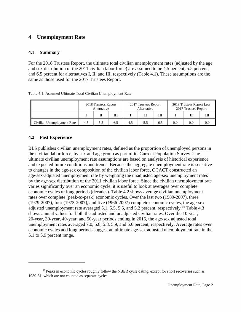
Unemployment Rate, Page 2
4 Unemployment Rate
4.1 Summary For the 2018 Trustees Report, the ultimate total civilian unemployment rates (adjusted by the age and sex distribution of the 2011 civilian labor force) are assumed to be 4.5 percent, 5.5 percent, and 6.5 percent for alternatives I, II, and III, respectively (Table 4.1). These assumptions are the same as those used for the 2017 Trustees Report. Table 4.1: Assumed Ultimate Total Civilian Unemployment Rate
2018 Trustees Report Alternative
2017 Trustees Report Alternative
2018 Trustees Report Less 2017 Trustees Report
I II III I II III I II III
Civilian Unemployment Rate 4.5 5.5 6.5 4.5 5.5 6.5 0.0 0.0 0.0
4.2 Past Experience BLS publishes civilian unemployment rates, defined as the proportion of unemployed persons in the civilian labor force, by sex and age group as part of its Current Population Survey. The ultimate civilian unemployment rate assumptions are based on analysis of historical experience and expected future conditions and trends. Because the aggregate unemployment rate is sensitive to changes in the age-sex composition of the civilian labor force, OCACT constructed an age-sex-adjusted unemployment rate by weighting the unadjusted age-sex unemployment rates by the age-sex distribution of the 2011 civilian labor force. Since the civilian unemployment rate varies significantly over an economic cycle, it is useful to look at averages over complete economic cycles or long periods (decades). Table 4.2 shows average civilian unemployment rates over complete (peak-to-peak) economic cycles. Over the last two (1989-2007), three (1979-2007), four (1973-2007), and five (1966-2007) complete economic cycles, the age-sex adjusted unemployment rate averaged 5.1, 5.5, 5.5, and 5.2 percent, respectively.56 Table 4.3 shows annual values for both the adjusted and unadjusted civilian rates. Over the 10-year, 20-year, 30-year, 40-year, and 50-year periods ending in 2016, the age-sex adjusted total unemployment rates averaged 7.0, 5.8, 5.8, 5.9, and 5.6 percent, respectively. Average rates over economic cycles and long periods suggest an ultimate age-sex adjusted unemployment rate in the 5.1 to 5.9 percent range.
56 Peaks in economic cycles roughly follow the NBER cycle dating, except for short recoveries such as 1980-81, which are not counted as separate cycles.
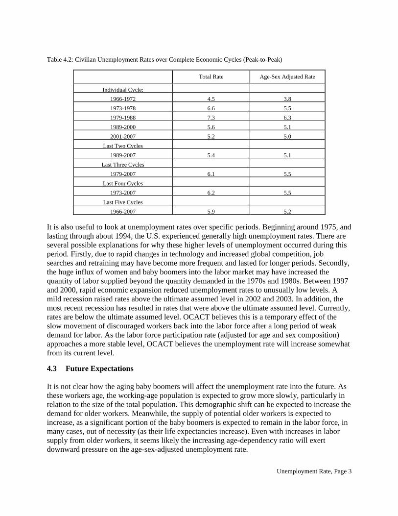
Unemployment Rate, Page 3
Table 4.2: Civilian Unemployment Rates over Complete Economic Cycles (Peak-to-Peak)
Total Rate Age-Sex Adjusted Rate
Individual Cycle: 1966-1972 4.5 3.8 1973-1978 6.6 5.5 1979-1988 7.3 6.3 1989-2000 5.6 5.1 2001-2007 5.2 5.0
Last Two Cycles 1989-2007
5.4 5.1 Last Three Cycles
1979-2007 6.1 5.5 Last Four Cycles
1973-2007 6.2 5.5 Last Five Cycles
1966-2007 5.9 5.2 It is also useful to look at unemployment rates over specific periods. Beginning around 1975, and lasting through about 1994, the U.S. experienced generally high unemployment rates. There are several possible explanations for why these higher levels of unemployment occurred during this period. Firstly, due to rapid changes in technology and increased global competition, job searches and retraining may have become more frequent and lasted for longer periods. Secondly, the huge influx of women and baby boomers into the labor market may have increased the quantity of labor supplied beyond the quantity demanded in the 1970s and 1980s. Between 1997 and 2000, rapid economic expansion reduced unemployment rates to unusually low levels. A mild recession raised rates above the ultimate assumed level in 2002 and 2003. In addition, the most recent recession has resulted in rates that were above the ultimate assumed level. Currently, rates are below the ultimate assumed level. OCACT believes this is a temporary effect of the slow movement of discouraged workers back into the labor force after a long period of weak demand for labor. As the labor force participation rate (adjusted for age and sex composition) approaches a more stable level, OCACT believes the unemployment rate will increase somewhat from its current level.
4.3 Future Expectations It is not clear how the aging baby boomers will affect the unemployment rate into the future. As these workers age, the working-age population is expected to grow more slowly, particularly in relation to the size of the total population. This demographic shift can be expected to increase the demand for older workers. Meanwhile, the supply of potential older workers is expected to increase, as a significant portion of the baby boomers is expected to remain in the labor force, in many cases, out of necessity (as their life expectancies increase). Even with increases in labor supply from older workers, it seems likely the increasing age-dependency ratio will exert downward pressure on the age-sex-adjusted unemployment rate.

Unemployment Rate, Page 4
OCACT expects slower rates of increase in female labor force participation, as their rates of labor force participation stabilize closer to, but generally below, those of their male counterparts. The expected slower growth in the labor supply in the future relative to the total population is expected to produce an age-sex adjusted unemployment rate below the 5.9 percent experienced over the last 40 years (1976-2016). OCACT believes it is more reasonable to expect that the ultimate future age-sex-adjusted unemployment rate will be slightly below the 5.6 level experienced over the last 50 years (1966-2016). Therefore, the assumed ultimate average unemployment rate is 5.5 percent (age-sex adjusted to the 2011 labor force) for alternative II.
4.4 Projections from Other Sources IHS Markit (formerly Global Insight, Inc.) provides projections through 2047 in its latest long-run trend forecast (see The 30-Year Focus, Third Quarter, August 2017). IHS Markit projects the civilian unemployment rate will be 4.7 percent in 2027 and 2047. The Moody’s Analytics’ September 2017 forecast shows a civilian unemployment rate of 5.8 percent in 2027 and 5.1 percent in 2047. The OMB Mid-Session Review of the 2018 Fiscal Year Budget includes projections through 2027. OMB projects an aggregate civilian unemployment rate of 4.8 percent for 2022 and later. The Congressional Budget Office (CBO) report, An Update to the Budget and Economic Outlook: 2017 to 2027 (published June 2017), includes projections through 2027. CBO projects an aggregate civilian unemployment rate of 4.9 percent for 2027. The Social Security Advisory Board’s 2015 Technical Panel on Assumptions and Methods recommended assuming an ultimate (i.e., long-range average) aggregate civilian unemployment rate of 5.5 percent for alternative II.
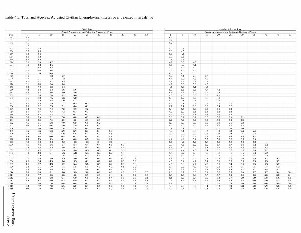
Unem
ployment R
ate, Page 5
Table 4.3: Total and Age-Sex Adjusted Civilian Unemployment Rates over Selected Intervals (%)
Year 1 5 10 15 20 25 30 35 40 45 50 1 5 10 15 20 25 30 35 40 45 501961 6.7 6.31962 5.5 5.21963 5.6 5.21964 5.2 4.71965 4.5 5.5 4.0 5.11966 3.8 4.9 3.3 4.51967 3.8 4.6 3.3 4.11968 3.5 4.2 3.0 3.61969 3.5 3.8 2.9 3.31970 5.0 3.9 4.7 4.2 3.3 4.21971 6.0 4.4 4.6 5.1 3.7 4.11972 5.6 4.7 4.7 4.7 4.0 4.01973 4.9 5.0 4.6 3.9 4.2 3.91974 5.6 5.4 4.6 4.5 4.5 3.91975 8.5 6.1 5.0 5.2 7.2 5.1 4.2 4.51976 7.7 6.5 5.4 5.2 6.4 5.3 4.5 4.51977 7.0 6.7 5.7 5.3 5.8 5.6 4.8 4.51978 6.1 7.0 6.0 5.4 4.9 5.8 5.0 4.51979 5.8 7.0 6.2 5.4 4.7 5.8 5.1 4.51980 7.2 6.8 6.4 5.6 5.6 5.9 5.6 5.3 4.7 4.81981 7.6 6.7 6.6 5.9 5.6 6.3 5.5 5.4 4.9 4.81982 9.7 7.3 7.0 6.2 5.8 8.3 6.0 5.8 5.2 4.91983 9.6 8.0 7.5 6.6 6.0 8.3 6.7 6.2 5.5 5.11984 7.5 8.3 7.7 6.9 6.1 6.5 7.1 6.4 5.8 5.21985 7.2 8.3 7.5 7.1 6.3 6.1 6.3 7.1 6.3 5.9 5.3 5.21986 7.0 8.2 7.5 7.1 6.4 6.1 6.1 7.1 6.3 6.0 5.4 5.21987 6.2 7.5 7.4 7.2 6.6 6.2 5.4 6.5 6.3 6.0 5.5 5.21988 5.5 6.7 7.3 7.2 6.7 6.2 4.9 5.9 6.3 6.1 5.6 5.21989 5.3 6.2 7.3 7.2 6.7 6.2 4.7 5.5 6.3 6.1 5.7 5.21990 5.6 5.9 7.1 7.0 6.8 6.2 6.1 5.0 5.2 6.2 6.0 5.7 5.3 5.21991 6.8 5.9 7.0 6.9 6.8 6.3 6.1 6.2 5.2 6.2 6.0 5.8 5.4 5.21992 7.5 6.1 6.8 7.0 6.9 6.5 6.2 6.9 5.5 6.0 6.0 5.9 5.5 5.31993 6.9 6.4 6.6 7.0 7.0 6.6 6.2 6.4 5.9 5.9 6.1 6.0 5.7 5.31994 6.1 6.6 6.4 7.0 7.0 6.7 6.2 5.7 6.1 5.8 6.2 6.1 5.8 5.41995 5.6 6.6 6.3 6.9 6.9 6.7 6.3 6.2 5.2 6.1 5.7 6.2 6.0 5.8 5.4 5.41996 5.4 6.3 6.1 6.8 6.8 6.7 6.3 6.1 5.0 5.8 5.5 6.1 5.9 5.8 5.5 5.31997 4.9 5.8 6.0 6.5 6.7 6.7 6.4 6.1 4.6 5.4 5.5 5.8 5.9 5.8 5.5 5.31998 4.5 5.3 5.9 6.1 6.6 6.7 6.4 6.1 4.2 4.9 5.4 5.5 5.8 5.8 5.5 5.31999 4.2 4.9 5.8 5.9 6.5 6.6 6.4 6.0 3.9 4.6 5.3 5.4 5.8 5.8 5.6 5.32000 4.0 4.6 5.6 5.7 6.4 6.4 6.4 6.0 6.0 3.7 4.3 5.2 5.2 5.7 5.7 5.6 5.2 5.22001 4.8 4.5 5.4 5.6 6.2 6.3 6.3 6.1 5.9 4.5 4.2 5.0 5.1 5.6 5.6 5.5 5.3 5.22002 5.8 4.6 5.2 5.5 6.0 6.3 6.3 6.1 5.9 5.5 4.4 4.9 5.1 5.5 5.6 5.6 5.3 5.22003 6.0 4.9 5.1 5.6 5.8 6.3 6.4 6.2 5.9 5.8 4.7 4.8 5.2 5.3 5.6 5.6 5.4 5.22004 5.5 5.2 5.1 5.6 5.7 6.3 6.4 6.2 5.9 5.3 5.0 4.8 5.2 5.3 5.6 5.7 5.5 5.22005 5.1 5.4 5.0 5.5 5.6 6.2 6.3 6.2 6.0 5.9 4.9 5.2 4.8 5.2 5.2 5.6 5.6 5.5 5.2 5.22006 4.6 5.4 4.9 5.4 5.5 6.1 6.2 6.2 6.0 5.9 4.5 5.2 4.7 5.1 5.1 5.5 5.5 5.5 5.3 5.22007 4.6 5.2 4.9 5.2 5.4 5.8 6.1 6.2 6.0 5.8 4.5 5.0 4.7 4.9 5.1 5.4 5.5 5.5 5.3 5.22008 5.8 5.1 5.0 5.1 5.5 5.7 6.1 6.2 6.1 5.8 5.7 5.0 4.8 4.9 5.1 5.3 5.5 5.5 5.4 5.22009 9.3 5.9 5.5 5.3 5.7 5.8 6.2 6.3 6.2 5.9 9.2 5.8 5.4 5.1 5.3 5.4 5.7 5.7 5.5 5.32010 9.6 6.8 6.1 5.6 5.9 5.9 6.3 6.3 6.3 6.0 6.0 9.6 6.7 6.0 5.4 5.6 5.5 5.8 5.7 5.7 5.4 5.42011 8.9 7.7 6.5 5.8 6.0 5.9 6.3 6.4 6.4 6.2 6.0 8.9 7.6 6.4 5.7 5.7 5.6 5.9 5.8 5.8 5.5 5.42012 8.1 8.3 6.8 6.1 6.0 6.0 6.3 6.4 6.5 6.3 6.1 8.1 8.3 6.7 5.9 5.8 5.7 5.9 5.9 5.8 5.6 5.52013 7.4 8.7 6.9 6.2 6.0 6.1 6.2 6.4 6.5 6.3 6.1 7.4 8.6 6.8 6.1 5.8 5.8 5.8 6.0 5.9 5.7 5.52014 6.2 8.0 7.0 6.4 6.0 6.1 6.1 6.5 6.5 6.4 6.1 6.2 8.0 6.9 6.3 5.8 5.9 5.8 6.0 6.0 5.8 5.62015 5.3 7.2 7.0 6.5 6.0 6.1 6.1 6.4 6.4 6.4 6.2 5.3 7.2 6.9 6.4 5.8 5.9 5.8 6.0 5.9 5.8 5.62016 4.9 6.3 7.0 6.5 6.0 6.0 6.0 6.3 6.4 6.4 6.2 4.9 6.4 7.0 6.4 5.8 5.8 5.7 5.9 5.9 5.8 5.6
Total Rate Age-Sex Adjusted RateAnnual Average over the Following Number of Years Annual Average over the Following Number of Years
Annual Trust Fund Real Interest Rate, Page 1
5. ANNUAL TRUST FUND REAL INTEREST RATE
THE 2018 TRUSTEES REPORT OFFICE OF THE CHIEF ACTUARY, SOCIAL SECURITY ADMINISTRATION
TABLE OF CONTENTS PAGE
5 ANNUAL TRUST FUND REAL INTEREST RATE ......................................................... 2 5.1 SUMMARY ...................................................................................................................................................... 2 5.2 PAST EXPERIENCE .......................................................................................................................................... 2 5.3 FUTURE EXPECTATIONS ................................................................................................................................. 4 5.4 PROJECTIONS FROM OTHER SOURCES ............................................................................................................. 5
TABLE OF TABLES PAGE TABLE 5.1: ASSUMED ULTIMATE REAL INTEREST RATES .............................................................................................. 2 TABLE 5.2: AVERAGE ANNUAL REAL INTEREST RATE (CALCULATED USING THE ADJUSTED-CPIW) ............................. 3 TABLE 5.3: REAL INTEREST RATES FOR OASDI TRUST FUND NEW ISSUES AND THE COMPOUND AVERAGE REAL
YIELD OVER SELECTED INTERVALS ........................................................................................................................ 7
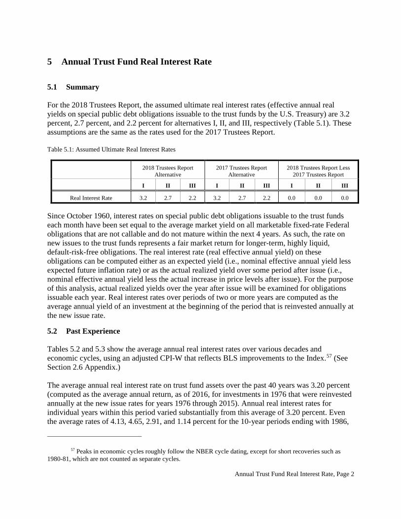
Annual Trust Fund Real Interest Rate, Page 2
5 Annual Trust Fund Real Interest Rate
5.1 Summary For the 2018 Trustees Report, the assumed ultimate real interest rates (effective annual real yields on special public debt obligations issuable to the trust funds by the U.S. Treasury) are 3.2 percent, 2.7 percent, and 2.2 percent for alternatives I, II, and III, respectively (Table 5.1). These assumptions are the same as the rates used for the 2017 Trustees Report. Table 5.1: Assumed Ultimate Real Interest Rates
2018 Trustees Report Alternative
2017 Trustees Report Alternative
2018 Trustees Report Less 2017 Trustees Report
I II III I II III I II III
Real Interest Rate 3.2 2.7 2.2 3.2 2.7 2.2 0.0 0.0 0.0
Since October 1960, interest rates on special public debt obligations issuable to the trust funds each month have been set equal to the average market yield on all marketable fixed-rate Federal obligations that are not callable and do not mature within the next 4 years. As such, the rate on new issues to the trust funds represents a fair market return for longer-term, highly liquid, default-risk-free obligations. The real interest rate (real effective annual yield) on these obligations can be computed either as an expected yield (i.e., nominal effective annual yield less expected future inflation rate) or as the actual realized yield over some period after issue (i.e., nominal effective annual yield less the actual increase in price levels after issue). For the purpose of this analysis, actual realized yields over the year after issue will be examined for obligations issuable each year. Real interest rates over periods of two or more years are computed as the average annual yield of an investment at the beginning of the period that is reinvested annually at the new issue rate.
5.2 Past Experience Tables 5.2 and 5.3 show the average annual real interest rates over various decades and economic cycles, using an adjusted CPI-W that reflects BLS improvements to the Index.57 (See Section 2.6 Appendix.) The average annual real interest rate on trust fund assets over the past 40 years was 3.20 percent (computed as the average annual return, as of 2016, for investments in 1976 that were reinvested annually at the new issue rates for years 1976 through 2015). Annual real interest rates for individual years within this period varied substantially from this average of 3.20 percent. Even the average rates of 4.13, 4.65, 2.91, and 1.14 percent for the 10-year periods ending with 1986,
57 Peaks in economic cycles roughly follow the NBER cycle dating, except for short recoveries such as 1980-81, which are not counted as separate cycles.
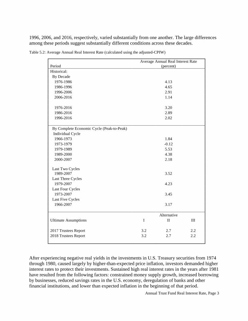
Annual Trust Fund Real Interest Rate, Page 3
1996, 2006, and 2016, respectively, varied substantially from one another. The large differences among these periods suggest substantially different conditions across these decades.
Table 5.2: Average Annual Real Interest Rate (calculated using the adjusted-CPIW)
Period Average Annual Real Interest Rate
(percent) Historical: By Decade 1976-1986 4.13 1986-1996 4.65 1996-2006 2.91 2006-2016 1.14 1976-2016 3.20 1986-2016 2.89 1996-2016 2.02 By Complete Economic Cycle (Peak-to-Peak) Individual Cycle 1966-1973 1.84 1973-1979 -0.12 1979-1989 5.53 1989-2000 4.38 2000-2007 2.18 Last Two Cycles 1989-2007 3.52 Last Three Cycles 1979-2007 4.23 Last Four Cycles 1973-2007 3.45 Last Five Cycles 1966-2007 3.17 Alternative Ultimate Assumptions I II III 2017 Trustees Report 3.2 2.7 2.2 2018 Trustees Report 3.2 2.7 2.2
After experiencing negative real yields in the investments in U.S. Treasury securities from 1974 through 1980, caused largely by higher-than-expected price inflation, investors demanded higher interest rates to protect their investments. Sustained high real interest rates in the years after 1981 have resulted from the following factors: constrained money supply growth, increased borrowing by businesses, reduced savings rates in the U.S. economy, deregulation of banks and other financial institutions, and lower than expected inflation in the beginning of that period.
Annual Trust Fund Real Interest Rate, Page 4
As the rate of inflation declined from the highs of the early 1980s and remained under control, the real interest rate slowly followed suit, declining to 2.34 percent in 2000. In October 2001, the federal government, in response to its favorable budget situation, suspended the sale of 30-year Treasury securities (leaving the 10-year notes as the longest duration being issued). Since then, the budget has fallen back into deficit and, beginning in February 2006, the Treasury re-introduced regular semi-annual auctions of the 30-year nominal Treasury bond. Neither the budget deficits nor the federal funds rate hikes by the Federal Reserve between 2004 and 2006 have resulted in a spike in real interest rates, due in part to foreigners’ increased willingness to accumulate Treasury securities. Instead, the real interest rate continued to trend downward, reaching 0.63 percent in 2008. Since 2008, the annual real interest rate has averaged only 1.11 percent, largely due to slow economic growth, unconventional monetary policies such as quantitative easing, a global savings glut, as well as a strong demand for safe assets in order to satisfy regulatory requirements in the financial sector.
5.3 Future Expectations Real interest rates have been unusually low during the 2000-2016 period, and are not expected to remain low in the future. Real interest rates were unusually low during the 2000-2007 as rates were distorted by large purchases of safe assets (including Treasury securities) by foreign central banks as their foreign exchange reserves accumulated. The low interest rates helped fuel the housing bubble, and when the bubble burst in 2007, investors sought a safe haven in Treasury securities. The sluggish economic growth in the United States together with financial instability abroad contributed to the low real interest rates in the post-2009 period. In addition, during most of this period, foreign central banks continued to accumulate foreign exchange reserves, which also contributed to the low real interest rates. While foreigners have recently become net sellers of Treasury securities, US financial institutions’ demand for Treasury securities has increased in order to satisfy their regulatory requirement that they hold sufficient high-quality liquid assets, such as Treasury securities. Over the near term, yields on Treasury securities can be expected to rise moderately as long as the economy continues to improve and the Federal Reserve continues with its interest rate normalization process. The Federal Reserve, which ended its asset-purchase program (quantitative easing) in October 2014, has raised its Federal funds rate four times since December 2015, and started its balance sheet normalization process in October 2017 by gradually reducing its securities holdings. This balance sheet normalization process is expected to continue as long as the economy continues to grow as anticipated and should put upward pressure on longer-term interest rates. Over the longer term, several factors are expected to result in higher yields on Treasury securities. First, the CBO projects that budget deficits will exceed one trillion dollars by 2022. By 2027, CBO projects the amount of publicly held debt will exceed 91 percent of GDP. The high level of debt may eventually lead to sharp and sudden increases in the yields on Treasury securities. Second, efforts are underway to reduce regulatory requirements for financial institutions that were put in place following the most recent recession, which may reduce the

Annual Trust Fund Real Interest Rate, Page 5
demand for safe assets such as Treasuries. Third, continued growth in the global economy may reduce the demand for safe assets such as Treasury securities. In recent years, term structure models have become popular and are used to decompose the long-term interest rate into a short-term interest rate and a term premium. Unfortunately, a study by the Congressional Budget Office58 found that yield-curve-based models have been worse predictors of long-term interest rates than the Blue Chip consensus forecasts over the past three decades. Moreover, even the Blue Chip consensus forecasts failed to predict the declining long-term interest rates over that period. When determining the assumed ultimate real interest rate for the long-range period, OCACT believes it is important to take into consideration the real interest rates experienced over long historical periods as well as whether or not the relatively low real interest rates experienced in the recent past can continue well into the long-range period. Over the last five economic cycles (1966-2007), which included the 2000-2007 cycle during which real interest rates averaged only 2.18 percent, the real interest rate averaged 3.17 percent. Even if only the post-1987 period (through 2016) is considered, the real interest rate averaged 2.83 percent while the CPI growth rate averaged 2.4 percent. The low real interest rates experienced in the 2007-2016 period (averaging 1.06 percent) do not make a compelling case for significantly changing the ultimate assumptions. Thus, the Trustees maintain the ultimate real interest rate assumption at 3.2 percent, 2.7 percent and 2.2 percent for alternatives I, II and III, respectively. However, should the government debt in the future grow to a level higher than what investors are willing to absorb, then a higher real interest rate assumption would be reasonable.
5.4 Projections from Other Sources IHS Markit (formerly IHS Global Insight, Inc.) includes projections through 2047 in its August 2017 30-Year Focus Trend Forecast. They project real yields on 10-year U.S. Treasury notes to rise from 0.7 percent for 2018 to an ultimate rate in the 1.6 to 1.7 percent range for 2028 and thereafter. Moody’s Analytics’ September 2017 forecast projects real yields on 10-year U.S. Treasury notes to rise from 0.5 percent in 2018 to an ultimate rate of 1.9 percent for 2039 through 2047 (their final projection year). Macroeconomic Advisers produces forecasts to 2025 only. The Office of Management and Budget (OMB) Fiscal Year 2018 Budget projects the real yield on the trust funds’ special-issue securities to reach 1.6 percent by 2023 and remain at that level for the remainder of the projection period (through 2095). The Congressional Budget Office (CBO) 2017 Long-Term Budget Outlook (published March 2017) includes projections through 2091. CBO projects real yields on 10-year Treasury notes of 2.3 percent in 2046 and later. The
58 CBO, “Did Treasury Debt Markets Anticipate the Persistent Decline in Long-Term Interest Rates?”,
Working Paper 2017-07. https://www.cbo.gov/publication/53153
Annual Trust Fund Real Interest Rate, Page 6
Social Security Advisory Board’s 2015 Technical Panel on Assumptions and Methods recommended lowering the alternative II real interest rate assumption to 2.5 percent. The prior technical panel, which met in 2011, recommended lowering the alternative II real interest rate assumption to 2.7 percent.
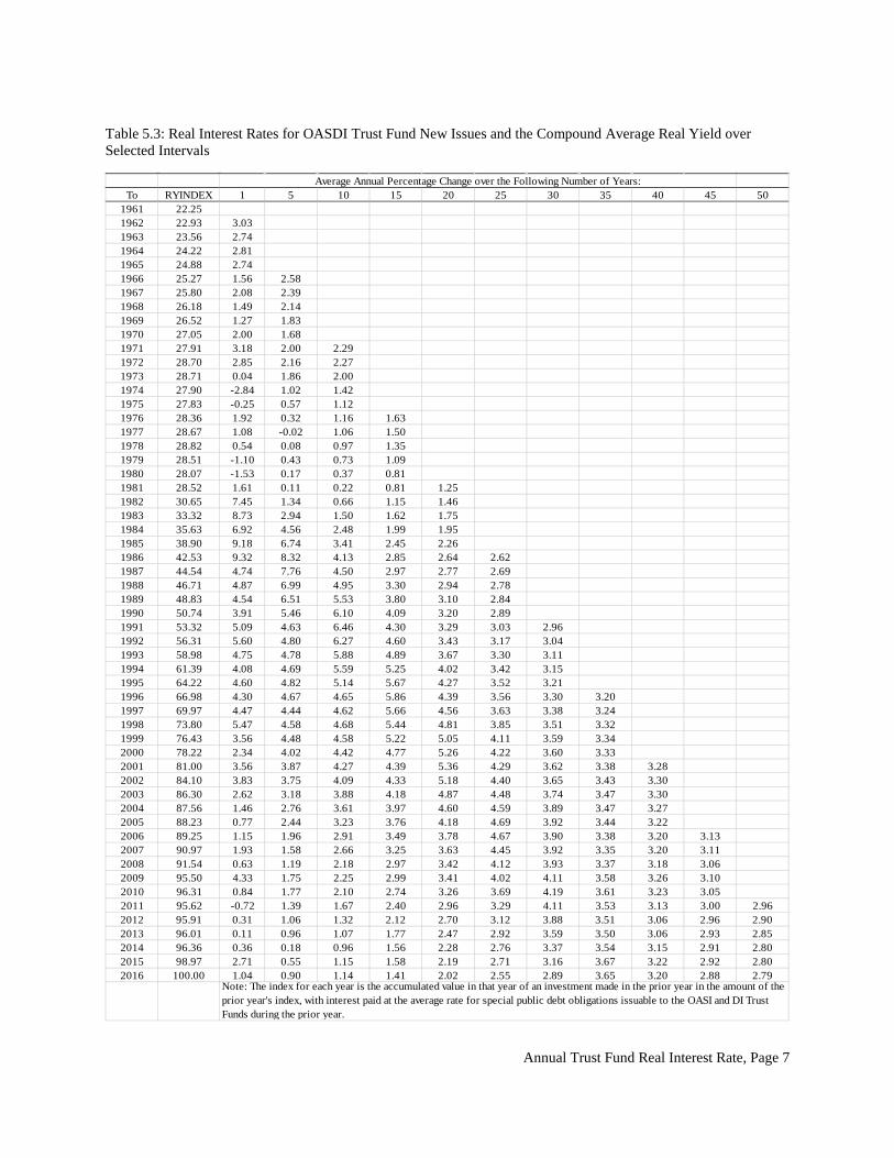
Annual Trust Fund Real Interest Rate, Page 7
Table 5.3: Real Interest Rates for OASDI Trust Fund New Issues and the Compound Average Real Yield over Selected Intervals
To RYINDEX 1 5 10 15 20 25 30 35 40 45 501961 22.251962 22.93 3.031963 23.56 2.741964 24.22 2.811965 24.88 2.741966 25.27 1.56 2.581967 25.80 2.08 2.391968 26.18 1.49 2.141969 26.52 1.27 1.831970 27.05 2.00 1.681971 27.91 3.18 2.00 2.291972 28.70 2.85 2.16 2.271973 28.71 0.04 1.86 2.001974 27.90 -2.84 1.02 1.421975 27.83 -0.25 0.57 1.121976 28.36 1.92 0.32 1.16 1.631977 28.67 1.08 -0.02 1.06 1.501978 28.82 0.54 0.08 0.97 1.351979 28.51 -1.10 0.43 0.73 1.091980 28.07 -1.53 0.17 0.37 0.811981 28.52 1.61 0.11 0.22 0.81 1.251982 30.65 7.45 1.34 0.66 1.15 1.461983 33.32 8.73 2.94 1.50 1.62 1.751984 35.63 6.92 4.56 2.48 1.99 1.951985 38.90 9.18 6.74 3.41 2.45 2.261986 42.53 9.32 8.32 4.13 2.85 2.64 2.621987 44.54 4.74 7.76 4.50 2.97 2.77 2.691988 46.71 4.87 6.99 4.95 3.30 2.94 2.781989 48.83 4.54 6.51 5.53 3.80 3.10 2.841990 50.74 3.91 5.46 6.10 4.09 3.20 2.891991 53.32 5.09 4.63 6.46 4.30 3.29 3.03 2.961992 56.31 5.60 4.80 6.27 4.60 3.43 3.17 3.041993 58.98 4.75 4.78 5.88 4.89 3.67 3.30 3.111994 61.39 4.08 4.69 5.59 5.25 4.02 3.42 3.151995 64.22 4.60 4.82 5.14 5.67 4.27 3.52 3.211996 66.98 4.30 4.67 4.65 5.86 4.39 3.56 3.30 3.201997 69.97 4.47 4.44 4.62 5.66 4.56 3.63 3.38 3.241998 73.80 5.47 4.58 4.68 5.44 4.81 3.85 3.51 3.321999 76.43 3.56 4.48 4.58 5.22 5.05 4.11 3.59 3.342000 78.22 2.34 4.02 4.42 4.77 5.26 4.22 3.60 3.332001 81.00 3.56 3.87 4.27 4.39 5.36 4.29 3.62 3.38 3.282002 84.10 3.83 3.75 4.09 4.33 5.18 4.40 3.65 3.43 3.302003 86.30 2.62 3.18 3.88 4.18 4.87 4.48 3.74 3.47 3.302004 87.56 1.46 2.76 3.61 3.97 4.60 4.59 3.89 3.47 3.272005 88.23 0.77 2.44 3.23 3.76 4.18 4.69 3.92 3.44 3.222006 89.25 1.15 1.96 2.91 3.49 3.78 4.67 3.90 3.38 3.20 3.132007 90.97 1.93 1.58 2.66 3.25 3.63 4.45 3.92 3.35 3.20 3.112008 91.54 0.63 1.19 2.18 2.97 3.42 4.12 3.93 3.37 3.18 3.062009 95.50 4.33 1.75 2.25 2.99 3.41 4.02 4.11 3.58 3.26 3.102010 96.31 0.84 1.77 2.10 2.74 3.26 3.69 4.19 3.61 3.23 3.052011 95.62 -0.72 1.39 1.67 2.40 2.96 3.29 4.11 3.53 3.13 3.00 2.962012 95.91 0.31 1.06 1.32 2.12 2.70 3.12 3.88 3.51 3.06 2.96 2.902013 96.01 0.11 0.96 1.07 1.77 2.47 2.92 3.59 3.50 3.06 2.93 2.852014 96.36 0.36 0.18 0.96 1.56 2.28 2.76 3.37 3.54 3.15 2.91 2.802015 98.97 2.71 0.55 1.15 1.58 2.19 2.71 3.16 3.67 3.22 2.92 2.802016 100.00 1.04 0.90 1.14 1.41 2.02 2.55 2.89 3.65 3.20 2.88 2.79
Average Annual Percentage Change over the Following Number of Years:
Note: The index for each year is the accumulated value in that year of an investment made in the prior year in the amount of the prior year's index, with interest paid at the average rate for special public debt obligations issuable to the OASI and DI Trust Funds during the prior year.

Ratio of OASDI Taxable Payroll to Covered Earnings, Page 1
6. RATIO OF OASDI TAXABLE PAYROLL TO COVERED EARNINGS
THE 2018 TRUSTEES REPORT OFFICE OF THE CHIEF ACTUARY, SOCIAL SECURITY ADMINISTRATION
TABLE OF CONTENTS PAGE 6 RATIO OF OASDI TAXABLE PAYROLL TO COVERED EARNINGS ...................... 2
6.1 SUMMARY ...................................................................................................................................................... 2 6.2 PAST EXPERIENCE .......................................................................................................................................... 2 6.3 FUTURE EXPECTATIONS ................................................................................................................................. 3 6.4 PROJECTIONS FROM OTHER SOURCES ............................................................................................................. 4
TABLE OF TABLES PAGE TABLE 6.1: ASSUMED ULTIMATE TAXABLE EARNINGS RATIOS ..................................................................................... 2 TABLE 6.2 OASDI TAXABLE RATIO, 1983 TO 2016 ....................................................................................................... 5 TABLE OF FIGURES PAGE FIGURE 6.1: PERCENTAGE OF OASDI COVERED EARNINGS BELOW THE TAXABLE MAXIMUM: 1983 TO 2016 .............. 3
Ratio of OASDI Taxable Payroll to Covered Earnings, Page 2
6 Ratio of OASDI Taxable Payroll to Covered Earnings
6.1 Summary For the 2018 Trustees Report, the assumed ultimate ratios of OASDI effective taxable payroll to covered earnings (taxable ratio) are 84.0 percent, 82.5 percent, and 81.0 percent for alternatives I, II and III, respectively (Table 6.1). These assumed ultimate ratios are the same as those used for the 2017 Trustees Report.
Table 6.1: Assumed Ultimate Taxable Earnings Ratios
2018 Trustees Report Alternative
2017 Trustees Report Alternative
2018 Trustees Report Less 2017 Trustees Report
I II III I II III I II III
Taxable Ratio (percent) 84.0 82.5 81.0 84.0 82.5 81.0 0.0 0.0 0.0
OASDI effective taxable payroll (or taxable payroll) is the effective amount of covered earnings subject to the full Social Security payroll tax rate (12.4 percent since 1990). Taxable wages for an employee are the total covered wages from all wage employment up to the taxable maximum (also known as the.contribution and benefit base). Taxable wages for an employer are the sum of all covered wages paid to each employee up to the taxable maximum. Employees with multiple jobs whose total wages exceed the taxable maximum are eligible for a refund of excess employee taxes withheld; employers are not eligible for a refund on this basis. For self-employed workers with no taxable wages, taxable earnings are the amount of covered self-employment net earnings up the taxable maximum. For self-employed workers with taxable wages, covered self-employment net earnings are taxable up to the excess (if any) of the taxable maximum over their taxable wages for the year. The taxable ratio is essentially the proportion of covered earnings that is at or below the taxable maximum.
6.2 Past Experience The taxable ratio fell from over 89 percent in 1983 to 84.3 percent in 2001, resulting in an average annual rate of change in the taxable ratio of about -0.34 percent (see Figure 6.1). The decline was related to several factors that increased the concentration of earnings among the very high earners compared to all other earners. Some of the drop in the taxable ratio in the late 1980s was due to the Tax Reform Act of 1986, which lowered the top marginal income tax rate from 50 percent in 1986 to 28 percent in 1988. The drop in the income tax rate influenced some high earners to shift some non-covered income to covered earnings, thereby lowering the taxable ratio. In the 1990s, the growth in the use of stock options59 in the pay packages of the very high
59 Nonqualified stock options are subject to the OASDI tax. For more information on the tax treatment of stock options,
see publication by Grant Thornton’s G. Edgar Adkins, Jr., entitled “Taxation of Stock Options and Restricted Stock: the Basics and Beyond” (https://www.grantthornton.com/~/media/content-page-files/tax/pdfs/white-papers-survey-reports-articles/2013/Taxation-of-stock-options-Adkins.ashx.)
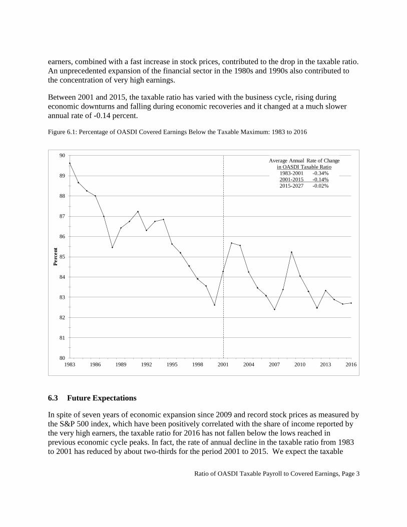
Ratio of OASDI Taxable Payroll to Covered Earnings, Page 3
earners, combined with a fast increase in stock prices, contributed to the drop in the taxable ratio. An unprecedented expansion of the financial sector in the 1980s and 1990s also contributed to the concentration of very high earnings.
Between 2001 and 2015, the taxable ratio has varied with the business cycle, rising during economic downturns and falling during economic recoveries and it changed at a much slower annual rate of -0.14 percent.
Figure 6.1: Percentage of OASDI Covered Earnings Below the Taxable Maximum: 1983 to 2016
6.3 Future Expectations In spite of seven years of economic expansion since 2009 and record stock prices as measured by the S&P 500 index, which have been positively correlated with the share of income reported by the very high earners, the taxable ratio for 2016 has not fallen below the lows reached in previous economic cycle peaks. In fact, the rate of annual decline in the taxable ratio from 1983 to 2001 has reduced by about two-thirds for the period 2001 to 2015. We expect the taxable
80
81
82
83
84
85
86
87
88
89
90
1983 1986 1989 1992 1995 1998 2001 2004 2007 2010 2013 2016
Perc
ent
Average Annual Rate of Changein OASDI Taxable Ratio1983-2001 -0.34%2001-2015 -0.14%2015-2027 -0.02%

Ratio of OASDI Taxable Payroll to Covered Earnings, Page 4
ratio will continue the trend of slowing decline in the near future and will stabilize to reach its ultimate value of 82.5 percent by the end of 2027 for the alternative II assumption.
6.4 Projections from Other Sources The Congressional Budget Office also makes projections of the taxable earnings ratio. In The 2017 Long-Term Budget Outlook published in March 2017, CBO projects the taxable ratio to fall from 82 percent in 2017 to 79 percent in 2027 and remain at that level thereafter (through 2047). One year earlier, in The 2016 Long-Term Budget Outlook, CBO projected the taxable ratio to fall to about 77.4 percent in 2027 and remain in the 77.4 to 77.5 percent range thereafter (through 2090).
The Social Security Advisory Board’s 2015 Technical Panel on Assumptions and Methods recommended lowering the alternative II ultimate taxable ratio from 82.5 percent to 82.2 percent. For alternatives I and III, the Technical Panel recommended ultimate taxable ratios of 84.0 percent and 79.0 percent, respectively. The 2011 Technical Panel recommended ultimate taxable ratios of 84.3 percent, 82.2 percent, and 80.0 percent for alternatives I, II and III, respectively.
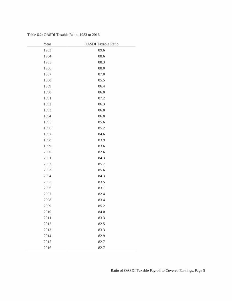
Ratio of OASDI Taxable Payroll to Covered Earnings, Page 5
Table 6.2: OASDI Taxable Ratio, 1983 to 2016
Year OASDI Taxable Ratio 1983 89.6 1984 88.6 1985 88.3 1986 88.0 1987 87.0 1988 85.5 1989 86.4 1990 86.8 1991 87.2 1992 86.3 1993 86.8 1994 86.8 1995 85.6 1996 85.2 1997 84.6 1998 83.9 1999 83.6 2000 82.6 2001 84.3 2002 85.7 2003 85.6 2004 84.3 2005 83.5 2006 83.1 2007 82.4 2008 83.4 2009 85.2 2010 84.0 2011 83.3 2012 82.5 2013 83.3 2014 82.9 2015 82.7 2016 82.7