The Long-Run Impacts of Special Education

Briana Ballis† and Katelyn Heath*

October 24, 2019

Latest version available at: https://brianaballis.weebly.com

Abstract

Over 13 percent of US students participate in Special Education (SE) programs annually, at a cost of$40 billion. However, the effect of SE placements remains unclear. This paper uses administrativedata from Texas to examine the long-run effect of reducing SE access. Our research design exploitsvariation in SE placement driven by a state policy that required school districts to reduce SEcaseloads to 8.5 percent. We show that this policy led to sharp reductions in SE enrollment. Thesereductions in SE access generated significant reductions in educational attainment, suggesting thatmarginal participants experience long-run benefits from SE services.

† University of California, Davis. Department of Economics. Email: bmballis@ucdavis.edu. * Cornell University.Department of Economics. Email: kmh324@cornell.edu.

We thank Scott Carrell, Paco Martorell, Marianne Page, Marianne Bitler, Maria Fitzpatrick, Michael Lovenheim,Douglas Miller, Jordan Matsudaira, Michal Kurlaender, and Jacob Hibel for useful discussions and suggestions. Wewould like to thank participants at the UC Davis Applied Microeconomics Brown Bag, the Association for EducationFinance and Policy 43rd Annual Conference, the UC Davis Alumni conference, the Western Economic AssociationInternational 93rd Annual Conference, the 40th annual Association for Public Policy Analysis and ManagementConference, and Claremont McKenna - Southern California Conference in Applied Microeconomics (SoCCAM) forvaluable comments. We also thank everyone at the UT Dallas Research Center who have helped us get acquainted withthe administrative data. The conclusions of this research do not necessarily reflect the opinions or official positionof the Texas Education Agency, the Texas Higher Education Coordinating Board, the Texas Workforce Commission,or the state of Texas. This material is based upon work supported by the National Science Foundation under GrantNumber (#1824547). Any opinions, findings, and conclusions or recommendations expressed in this material are thoseof the author(s) and do not necessarily reflect the views of the National Science Foundation. This project receivedsupport from the Social Security Administration (SSA) funded as part of the Disability Research Consortium. Theopinions and conclusions expressed are solely those of the authors and do not represent the opinions or policy ofSSA or any agency of the Federal Government. Briana Ballis acknowledges financial support from the DisabilityResearch Consortium Fellowship from SSA via Mathematica Policy, the National Science Foundation, and the UCDavis Economics department. Katelyn Heath acknowledges financial support from the National Academy of Educationand the National Academy of Education/Spencer Dissertation Fellowship Program, the Bronfenbrenner Center forTranslational Research, Christopher Wildeman, Cornell University Graduate School, Cornell Policy Analysis andManagement Department, and the Cornell Economics department Labor Grant. All errors are our own.

1 IntroductionSpecial Education (SE) program participation grew by over 40 percent between 1975 and 2018.

Currently, over 13 percent of public school students participate in SE programs annually, at a cost

of $40 billion (National Center for Education Statistics, 2015; Elder, Figlio, Imberman, & Persico,

2019). While the purpose of SE is to ameliorate the challenges students with disabilities may face

throughout schooling and later in life, considerable uncertainty surrounds the effectiveness of SE

spending. On the one hand, students are likely to benefit from the individualized educational support

(such as one-on-one tutoring, a classroom aide, therapy, or standardized testing modifications) that

SE offers. But for students with less severe conditions there are several reasons why SE participation

could be harmful: being placed in segregated learning environments or held to relatively lower

expectations regarding achievement may inhibit long-run success.

Despite significant increases in SE participation for students with less severe conditions,

there is little consensus on how placement (or lack of) affects the long-run trajectories of marginal

participants. The main difficulty in evaluating the effectiveness of SE programs is identifying a

plausible counterfactual. Students are selected to participate in SE because teachers believe they are

at risk of low achievement or poor behavioral outcomes. However, because SE inclusion criteria are

neither straightforward nor standardized for students with less severe conditions, it is not possible to

exploit discontinuities in SE diagnostic criteria to identify the causal impacts of SE participation.1

Instead, exogenous changes in SE participation are required for causal identification. But because

SE eligibility rules were determined federally in 1975 (with very minor changes since) it is difficult

to identify variation in SE placement across locations or over time that is plausibly exogenous.

This paper provides evidence on the long-run effects of SE by exploiting a rare policy

change that introduced exogenous variation in SE participation for marginal participants. In

2005, the Texas Department of Education implemented a district-level SE enrollment target of1For the vast majority of SE students with learning or behavioral impairments, the most common symptoms are

poor academic performance or classroom behaviors. Since many students exhibit these symptoms occasionally, thereare inconsistencies in SE placement based on how teachers, parents, or diagnosticians perceive these symptoms.

1

8.5 percent. This policy led to an immediate drop in SE enrollment. Over the next ten years,

statewide SE enrollment declined by 4.5 percentage points, from 13 percent to 8.5 percent. By

2018, roughly 225,000 fewer students were enrolled in SE programs annually across the state.2 To

our knowledge, this is the first major policy change that caused such a large and sudden change

in SE participation for a large representative sample of students. Nearly 10 years after the policy

was implemented, the federal government determined that the 8.5 district target violated federal

disability law, which highlights why policies such as this one are so rare. We exploit this policy

change using administrative data from Texas that follow the universe of public school students into

adulthood, allowing us to provide the first long-run causal estimates of SE programs.

Our research design exploits the pre-policy variation in SE rates across districts, which

led to significant differences in policy pressure to reduce SE enrollment. To identify the direct

impacts of SE programs for students with disabilities, we focus on cohorts enrolled in SE before the

policy’s implementation and estimate the long-run effect of a reduction in SE access using two main

identification strategies.3 First, we use a difference-in-differences strategy that compares changes

in SE removal, educational attainment, and labor market outcomes across cohorts with different

amounts of expected school enrollment after 2005 in districts with lower versus higher pre-policy

SE rates. This strategy estimates the average effect of reducing overall access to SE for students

with disabilities. Second, we use exposure to the policy as an instrument for SE removal in an

instrumental variables (IV) framework. This second strategy allows us to identify the long-run

impacts of SE removal for students on the margin of SE placement decisions, precisely the group

for whom the net benefits of SE are most unclear.

The validity of our research design rests on the assumption that districts facing more

policy pressure had similar counterfactual trends as districts facing less pressure. Event study graphs2This is computed by multiplying total enrollment in Texas public schools in 2018 (roughly 5 million) by the 4.5

percentage point reduction in total SE enrollment that occurred post-policy.3This sample restriction ensures that all students in our sample will share the same underlying conditions. The

policy pressure to reduce SE enrollment significantly changes the incentives to classify marginal students, which in turnchanges the underlying conditions of SE students. As we will justify in Section 3.2, we focus on 5th grade SE cohorts.However, we demonstrate that our results are not sensitive to this grade cohort restriction.

2

demonstrate that the pre-policy district SE rate is uncorrelated with outcomes for cohorts who were

too old to have been enrolled in school under the policy. Thus, it is unlikely our results are being

driven by pre-trends. In addition, we show that changes in predicted outcomes and attrition are

both uncorrelated with pre-policy rates of SE enrollment. This suggests that endogenous changes in

district composition are not driving our results. For our IV approach to yield causal estimates of SE

removal for marginal students, we must additionally assume that the policy only impacted students

through changes in SE removal. We provide strong evidence in support of this exclusion restriction

assumption. While the policy led to significant increases in the likelihood of SE removal, it did not

generate other changes in instruction or resources for SE students.

Our results suggest that students who are denied access to SE services experience sig-

nificant declines in educational attainment. Our difference-in-differences estimates imply that SE

students enrolled in the average district experienced a 3.5 percentage points (or 12 percent) increase

in the likelihood of SE removal, a 1.9 percentage points (or 2.6 percent) decrease in the likelihood

of high school completion, and a 1.2 percentage points (or 3.7 percent) decrease in the likelihood of

college enrollment after the policy’s introduction.4 For students on the margin of SE placement

decisions, our IV estimates imply that SE removal decreases both high school completion and

college enrollment by 52.2 and 37.8 percentage points, respectively. Lower-income and minority

students experience larger increases in SE removal, and the negative impact of SE removal on

educational attainment are concentrated among these students. We do not find that SE removal

leads to significant declines in college degree attainment or earnings in the labor market, measured

shortly after high school graduation (six years later). However, it is likely that the longer run college

completion and employment effects may differ once these outcomes have time to fully realize.5

The large reductions in high school completion and college enrollment that we document suggest

that later life labor market outcomes are also likely to decline.4These effect sizes are computed for SE students fully exposed to the policy after 5th grade and enrolled in the

average school district that served 13 percent of their students in SE at baseline.5Among SE students, the wage differential across college enrollment decisions emerges roughly six years after high

school completion. This suggests that it may still be too early to measure these outcomes.

3

Why do marginal students (i.e. those with relatively mild conditions) experience such

large reductions in educational attainment after SE removal? Part of the explanation is mechanical.

SE students can satisfy modified high school graduation requirements, which may make educational

attainment easier. For instance, students enrolled in SE may be able to graduate from high school

without passing an exit exam, which is a typical high school graduation requirement. We find that

students denied access to SE are significantly more likely to take the high school exit exam and

significantly less likely to pass it. However, it is unlikely that changes in high school graduation

requirements alone are driving our results. For instance, SE students are also likely to benefit from

the additional resources and more focused attention they receive. We find that the long-run negative

impacts of SE removal are concentrated in lower-resourced districts. This highlights the potential

importance that additional SE resources provide, especially in districts with less available resources

to prepare students with special needs for adulthood. Finally, it is important to highlight that we are

inferring SE program effects based on SE removal. For students who are accustomed to receiving

additional support in school, the negative impacts of SE removal could be particularly pronounced.6

Credibly estimating the long-run impacts of SE programs is difficult due to data limitations

and the empirical challenges previously noted. The few studies that have examined SE access and

placement have largely focused on short run outcomes and mostly find positive effects. Various

identification strategies have been used in an attempt to account for the endogenous placement of

students into SE. For example, using within student changes, Hanushek, Kain, and Rivkin (2002)

find that SE participation improves math performance for students with mild learning and behavioral

conditions. Using strategic placement in SE due to an accountability change that placed pressure on

schools to improve overall student performance, Cohen (2007) finds that SE participation reduces

absenteeism for marginal low-achieving students.7 Only one paper (Prenovitz, 2017) finds that6Long-run responses to never participating in SE may not mirror the impacts of SE removal. For instance, those

never enrolled in SE do not incur any potential stigma associated with a disability label and do not become accustomedto additional supports during school. However, with our administrative data it is difficult to identify students on themargin of placement prior to a SE diagnosis.

7Cohen (2007) also finds suggestive evidence that SE placement reduces the probability of dropping out andimproves GPA but these results are not significant at conventional levels.

4

SE participation harms student achievement. However, this difference from prior studies is likely

driven by the context that she focuses on. Prenovitz (2017) infers SE program effects based on

the introduction of No Child Left Behind (NCLB) that held schools accountable for SE subgroup

performance. In this setting, schools faced incentives to assign SE to higher-achieving students and

remove SE services for lower-achieving students, resulting in strategic SE placements for students

most unlikely to benefit from SE. Moreover, these results offer little insight into the role of SE

participation on adult outcomes. To date, the only evidence on the long-run impacts of SE has been

descriptive and focused on small samples (Newman et al., 2011).

We contribute to the literature in several important ways. First, to our knowledge, we

offer the first long-run causal impacts of SE participation for marginal students. Second, our focus

on one of the largest and plausibly exogenous reductions in SE access allow us to isolate changes in

SE access without having to make strong identification assumptions. Finally, using population data

from Texas, a large and diverse state, we are able to estimate differential responses to SE access

across many subgroups. We find that less advantaged students and those in lower-resourced or

lower-performing districts are more negatively impacted by reduced SE access, suggesting that less

access to SE programs may serve to expand pre-existing gaps in later life outcomes among these

groups.

More broadly, our results speak to central questions of how to raise human capital for

vulnerable student populations. First, we add to the literature that investigates the best way to

allocate school resources. In particular, are targeted resources (such as those offered by SE) or

broader improvements in school quality (that affect all students) more effective at improving long-

run trajectories for at-risk groups? The closest related work by Setren (2019) finds that students with

mild disabilities experience large achievement gains when they transition to Boston charter schools

which reduce individualized instructional support (by removing students from SE), but offer higher

quality overall instruction than Boston public schools. However, whether effective charter schools

can be replicated is unclear. Our results suggest large returns to investing in specialized educational

5

support when overall improvements in school quality are not possible. A rough comparison suggests

that targeting additional educational resources to students with less severe disabilities offer returns

that are significantly larger than reducing classroom sizes or increasing teacher salaries, but similar

to early childhood programs such as Head Start or Perry-Preschool, which are commonly viewed as

highly effective interventions (Levin, Belfield, Muennig, & Rouse, 2007).8

Second, we provide new evidence to the literature on the timing of human capital invest-

ments. While a large amount of evidence points to early childhood (i.e. before age 5) as the critical

period to invest resources in vulnerable youth (Garces, Thomas, & Currie, 2002; Deming, 2009;

Schweinhart et al., 2005), significantly less is known about the efficacy of interventions later during

childhood. Our findings suggest that investing additional resources for vulnerable groups later

during childhood can offer similar returns as early childhood investments do.

2 Background

2.1 Special Education Programs

The Individuals with Disabilities Education Act (IDEA) requires public schools to provide all

students a “free and appropriate” education. Under IDEA, students with disabilities receive SE

services to facilitate success in school and later in life. In Texas, as well as in other states, SE

program eligibility depends on having a qualifying disability that adversely affects learning, as

determined by teachers and specialists. The SE process begins when a parent, teacher, or school

administrator requests that a student be evaluated for SE services. Once referred, a psychologist

or special education teacher evaluates whether a student qualifies for SE services. SE students

are re-evaluated once every three years (or sooner if a parent or teacher requests it). Typically

students are first referred to SE during elementary school and continue to qualify for SE throughout

their entire schooling. However, some students transition out of SE if a student no longer requires8For this cost/benefit analysis, we use the social cost of a high school drop-out suggested by Levin et. al (2007). See

Section 6 for more detail on the methodology used to compare the cost/benefit across programs.

6

additional educational support to be able to succeed in school.9

Participating students receive individualized services and accommodations aimed at

ameliorating the challenges they are likely to face throughout schooling and later in life. Because

of this individualization, what SE offers is wide-ranging. Students may receive instruction in

general education classrooms accompanied by a classroom aid, in resource rooms for part of the

school day, or in separate classrooms or schools entirely. Additionally, they may be eligible for

extra time on standardized exams or take modified exams, which test content below grade level.

Another important component of SE is the close tracking of goals in annual meetings with parents

and teachers. Initially, yearly academic or behavioral goals are developed and tracked, and as

students approach high school graduation the focus turns towards adulthood goals of either college

enrollment or employment.10

As previously noted, SE participation has grown significantly since 1975 (from 8 to

13 percent). These increases in SE participation have been driven by large increases in learning

disabilities, speech impairments, other health impairments (including ADHD), and emotional

disturbance. Altogether, these conditions, hereafter referred to as “malleable disabilities”, now

represent over 90 percent of total SE enrollment in Texas. Unlike conditions that are physical or

more cognitively severe, SE eligibility for these conditions often involve discretion on the part

of diagnosticians, teachers, and parents. First, because the most common symptoms for these

disabilities are poor academic performance and classroom behaviors, which many students exhibit

occasionally, there are inconsistencies in SE referrals (Kauffman, Hallahan, & Pullen, 2017).

Moreover, even after being referred, determining whether these conditions adversely affect learning

without additional support (the main SE inclusion criteria) can be subjective, as can determining

whether students should remain in SE over time (Association et al., 2013). This subjectivity9For instance, in our sample over 70 percent of SE students who are diagnosed during elementary school (as of 5th

grade) continue to participate in SE into high school.10This preparation for adulthood is called transition planning. Students who aim to enroll in college typically receive

guidance on which colleges they should apply to and which courses would best prepare them for college. Those focusedon employment typically receive guidance on apprenticeships or other career/technical courses that may be beneficialonce they enter the labor market. Specific examples of transition plans are included in Appendix Figures A.1 and A.2

7

underscores the empirical challenges involved in estimating the causal impact of SE participation.

2.2 Policy Background

In the 2004-05 academic year, Texas implemented the Performance Based Monitoring Analysis

System (PBMAS) to monitor SE programs in public schools. Under the PBMAS, districts received

annual reports, which included several indicators to monitor SE programs. Broadly, these indicators

were aimed at limiting SE participation, improving SE students’ academic and behavioral outcomes,

and reducing the amount of services and accommodations being provided to SE students (i.e.

reducing time spent in separate classrooms and modified test-taking). However, beyond introducing

strong downward pressure on SE enrollment, this policy did not introduce significant policy pressure

on districts to make other changes for SE students. At the time the policy was introduced, roughly

98 percent of districts met or nearly met policy thresholds related to behavioral and academic

outcomes and 80 percent of districts met or nearly met policy thresholds related to the services and

accommodations offered to SE students. In contrast, only 5 percent of districts met the thresholds

related to SE enrollment.11

In this paper, we focus on the policy pressure to reduce SE enrollment due to the intro-

duction of a district SE enrollment target of 8.5 percent. Under this policy, any district that served

more than 8.5 percent of their students in SE faced state interventions ranging in severity based

on a district’s distance above the target.12 Districts closer to the target were subject to developing

monitoring improvement plans, while those further away were subject to third party on-site moni-

toring visits (Texas Education Agency, 2016).13 The first PBMAS report was received by districts

in December of the 2004-05 academic year, and was met by a sharp decline in SE enrollment.14

11Panel A of Appendix Table A.1 provides more detail on the fraction of districts that met, nearly met, did not meet,or were far out of compliance in each of SE monitoring area.

12Appendix Figure A.3 shows the rating that each district was assigned based on their SE rate.13Despite minimal sanctions for districts closer to the target, districts responded strongly. Based on a series of

interviews featured in a Houston Chronicle investigation of this policy school administrators report taking this targetseriously. For instance, one special education director noted, “We live and die by compliance. You can ask any specialed director; they’ll say the same thing: We do what the Texas Education Agency (TEA) tells us” (Rosenthal, 2016).

14Because the first PBMAS report was received in the middle of the 2004-05 school year (i.e. December 2004), inwhat follows, we consider the 2005-06 academic year as the first post-policy year. This was the first academic yearwhere districts would have responded to the policy pressure to reduce SE enrollment.

8

Figure 1 demonstrates that while the fraction of students enrolled in SE programs was constant

during the five years prior to the SE enrollment target (2000-2005), there was a sharp decline during

the five years afterwards (2005-2010). The average district experienced a 4.5 percentage point drop

with the largest reductions for districts furthest from the target.

In order to utilize the introduction of this policy to study the long-run effects of SE

participation, it is important to establish that the introduction of the SE enrollment target was

exogenous. Importantly, it appears to have been introduced in response to an unexpected state

budget cut (Hill et al., 2004) rather than statewide trends in SE enrollment or expenditures. There

is strong anecdotal evidence that it was unanticipated by districts (Rosenthal, 2018) and Figure

1 shows little indication of pre-trends in SE enrollment in the period leading up to the policy’s

introduction. In addition, it is important to establish that exploiting the cross-district variation in the

pre-policy district SE rate will allow us to identify the effect of a reduction in SE access separate

from other changes for SE students. Despite the SE enrollment target being introduced as part of a

broader monitoring effort, it is unlikely districts would have made other changes for SE students

beyond reducing their access to SE programs. As previously noted, the policy pressure to make any

instructional changes beyond SE removal was minimal. Therefore, we assume that the introduction

of PBMAS impacted students only through reducing their access to SE programs. Reassuringly,

throughout the paper we demonstrate that the pressure to make other instructional changes for SE

students are not driving our results, in support of this assumption.

3 Data and Summary Statistics

3.1 Data Sources

We leverage restricted-access administrative data from the Texas Schools Project (TSP). These data

follow the universe of Texas public school students into adulthood, tracking key education and labor

market outcomes. Specifically, we start with student-level records from the Texas Education Agency

(TEA). These data contain records for all Texas public school students in grades K through 12,

9

including yearly information on demographics, academic, and behavioral outcomes.15 Importantly,

these data include information on annual SE program participation, as well as disability type, the

amount of time spent in resource rooms (i.e. receiving instruction in separate classrooms),16 and

whether students’ took the unmodified version of standardized exams. Thus, we are able to carefully

track changes in SE placement, as well as the types of accommodations being offered to students

over time. We link these student-level school records from TEA to post-secondary enrollment data

from the Texas Higher Education Coordinating Board (THECB), as well as to labor market earnings

from the Texas Workforce Commission (TWC). The THECB data include enrollment and degree

attainment information for all Texas universities and the TWC includes earnings records for all

Texas employees subject to the state unemployment system.

These administrative data are advantageous both in terms of the number of long-term

outcomes and the large sample size. One drawback of using administrative data from a single state

is that we cannot track people who leave Texas. However, outmigration from Texas is quite low.

Most people born in Texas remain in the state (Aisch, Gebeloff, & Quealy, 2014) and only 1.7

percent of Texas residents leave the state each year (White et al., 2016). In addition, we are able to

link a subset of our sample to the National Student Clearinghouse (NCS) data in order to determine

how often students attend college out of state. Only 1.7 percent of SE students enroll in college

outside of Texas within two years of their high school graduation.17

3.2 Sample Construction

To identify the impact of SE on student outcomes, we focus on students enrolled in SE prior to the

enactment of the target and infer program effects from policy-driven SE removals. In particular,15Our data does not include performance on modified versions of standardized exams. Because the policy significantly

reduced SE enrollment, the fraction of students observed in the achievement data will be increasing endogenouslyover time due to fewer students enrolled in SE students who have the option of taking the modified versions. Thisunderscores why we do not focus on the impact of SE removal on achievement as a primary outcome in this paper.

16Specifically, we observe whether students spent all day in regular classrooms (or mainstreamed), less than 50percent of the day in separate classrooms, or more than 50 percent of the day in separate classrooms.

17We demonstrate in Section 5.4 that our results are not sensitive to the inclusion of out of state college enrollment.When we focus the subset of students for whom we observe NSC data (i.e. 5th grade SE cohorts from 2001 through2005), models that include out of state college enrollment provide nearly identical estimates to our main estimateswhich only include college enrollment within Texas.

10

we focus on students enrolled in SE programs as of 5th grade. We focus on 5th grade SE cohorts

for several reasons. First, they capture a stable sample of SE students: as Appendix Figure A.4

makes clear, SE enrollment typically grows rapidly throughout elementary school and levels off

by 5th grade (with very little new enrollment afterwards). Moreover, 5th grade cohorts have many

remaining years in school making them more susceptible to the policy change than older cohorts

would have been.18

Our main analysis sample consists of 5th grade SE cohorts enrolled between 1999-00 and

2004-05. The 2004-05 cohort was the last cohort diagnosed before the SE enrollment target was

enforced in public schools.19 Since the policy significantly changed the composition of students

identified with disabilities, this cohort restriction is necessary in order to ensure that students in

our sample have similar underlying conditions. Unless otherwise specified, we also restrict the

earliest cohort to the 1999-00 cohort (rather than the 1995-96 cohort when our data begins). We

make this additional restriction in order to avoid including cohorts affected by the introduction of

school finance equalization in Texas that also affected SE classification incentives (Cullen, 2003).

In particular, Cullen (2003) demonstrates that school finance equalization increased fiscal incentives

to enroll marginal students in higher-wealth districts. By 1999-00, SE enrollment rates had leveled

off.20 Finally, we limit our sample to students in districts that served between 6.6 and 21.5 percent

of their students in SE in 2004-05 to focus on districts with typical rates of SE.21 The final sample

consists of roughly 40,000 SE students from each cohort, for a total of 227,555 students.

To examine a particularly vulnerable subgroup, we use information about one’s disability18However, our results are not sensitive to this grade cohort restriction. In Appendix Table A.9 we demonstrate that

the impact of SE removal for 4th and 6th grade cohorts provide similar estimates to 5th grade cohorts.19Our data reports SE participation as of October. Thus the 2004-05 cohort was enrolled in SE as of October 2004

prior to when districts received the first PBMAS report in December 2004.20While school finance equalization changed classification incentives, it led to relatively small changes in SE access.

As such, in Appendix Table A.9 we demonstrate that our results are largely unchanged if we use the the extendednumber of cohorts (i.e. 1995-96 - 2004-05) or use cohorts in our main analysis sample (i.e. 1999-00 - 2004-05). Thus,it is sometimes helpful to extend the number of 5th grade cohorts back to 1995-96. For instance, in our event-studyanalysis extending the number of cohorts back to 1995-96 allows us to provide more visual evidence of pre-trends. Ifwe use the 1995-96 as our oldest 5th grade cohort rather than the 1999-00 cohort, this will be clearly specified.

21This drops roughly 1% of the overall sample since district outliers with respect to SE rates are small. Wedemonstrate in Appendix Table A.9 that our results are nearly identical if these districts are included.

11

(measured as of 5th grade) to identify students whose diagnoses may have been easier to manipulate

under the policy. We classify students as being more vulnerable to the policy pressure to reduce SE

enrollment if they had a malleable disability (including learning disabilities, speech impairments,

other health impairments (includes ADHD), or emotional disturbance) and if they received more

than 50 percent of their instruction in general education classrooms at baseline.22 In what follows,

we refer to this subgroup as our “high-impact” sample consisting of 189,042 students.

3.3 Summary Statistics

Table 1 presents summary statistics for 5th grade cohorts enrolled between 1999-00 and 2004-05.

Columns 1 vs. 2 compare students not enrolled in SE to those who are as of 5th grade. Students in

SE are more likely to receive Free and Reduced-Price Lunch (FRL), are slightly more likely to be

enrolled in the English Language Learner (ELL) program, have lower performance on standardized

exams (conditional on taking the unmodified version of the tests), and have lower long-run outcomes

(i.e. less likely to graduate, enroll in college, and have lower early labor market outcomes). These

differences help to highlight the fact that raw comparisons between those who receive SE services

and those who do not will be biased due to negative selection into SE programs.

Column 2 of Table 1 demonstrates that 91 percent of SE students diagnosed by 5th

grade have malleable disabilities, the most common of which is a learning disability at 60 percent.

The majority of SE students, 84 percent, receive over 50 percent of their instruction in regular

classrooms and 30 percent take unmodified standardized exams. As previously noted, SE students

may transition out of SE programs if SE services are no longer appropriate. Columns 3 vs. 4

of Table 1 compare SE students who continue in SE to those removed by 9th grade. 5th grade

SE students who lose SE are less likely to receive FRL, less likely to participate in ELL, have

higher achievement on standardized exams, and better long-run outcomes.23 Nearly all students

who lose SE have malleable disabilities (98 percent) and require fewer modifications to the regular22The rationale for this restriction is that if students are receiving most of their instruction outside of general education

classrooms then they are likely to have more severe conditions which may make it more difficult to justify SE removal.23High school graduation is the one exception to this pattern which can likely be explained by accommodated

graduation requirements available only to SE students.

12

curriculum; over 97 percent receive over 50 percent of their instruction in regular classrooms and

60 percent take unmodified standardized tests. These differences highlight the positive selection

into SE removal; without exogenous changes in SE participation, comparisons between those who

continue in SE vs. those who lose SE will be biased due to positive selection into SE removal.

4 Empirical Strategy

4.1 Difference-in-Differences Estimates of the Policy on Outcomes

We first estimate the causal impact of the policy pressure to reduce SE enrollment on student

outcomes. The SE enrollment target was introduced in all districts at the same time, so it is not

possible to use cross-district variation in implementation date. Instead, we use differences in

treatment intensity, which varies across students in two ways. First, districts with higher pre-policy

rates of SE enrollment faced stronger policy pressure to reduce SE enrollment. Thus, any effect of

the policy should be increasing with a student’s district’s pre-policy SE enrollment rate.24 Second,

5th grade cohorts were differentially treated under the policy based on the remaining number of

years that they were expected to be enrolled in school after the policy’s introduction in 2004-05.

We start by estimating an event-study specification that allows us to identify the impact of

the policy for each 5th grade cohort separately as follows:

Yicd = g0 +2005

Âj=cmin

g j {c = j}⇥SERatePred +l1Xicd +l2Zdc + gd +fc + eicd (1)

where Yicd is an indicator for SE removal or a long-run outcome for student i in 5th grade cohort

c in district d. SERatePred is the fraction of SE students above the 8.5 percent target in a students’

5th grade district in the 2004-05 school year (the year before the policy was implemented)25 and is24While this district level treatment is continuous, it may be helpful to think about districts under more policy pressure

as forming the “treated” group, whereas, those under less pressure form the “control” group.25We assign policy exposure based on a student’s 5th grade district (which was determined pre-policy). This ensures

that our estimates will be free of bias from selection into districts under less policy pressure to reduce SE enrollment.

13

interacted with each 5th grade cohort indicator variables. We control for 5th grade district fixed

effects gd and 5th grade cohort fixed effects fc. The vector Xicd , includes a dummy for gender, race,

Free and Reduced-Price Lunch (FRL) status, English Language Learner (ELL) classification, gender-

race interactions, primary disability, unmodified exam indicator, and level of classroom inclusion,

all measured at baseline in 5th grade, in order to absorb differences by student demographics and

disability type. Further, to control for changes in district-level demographics, Zdc, includes the

district percent of students by racial group, FRL, ELL, and gender for the full student population

and for the SE student population all defined at baseline.26

The main variables of interest, g j, identify differences in outcomes across students in

districts with higher versus lower pre-policy SE rates for each 5th grade cohort separately. We begin

with this specification since it allows us to directly test our main identification assumption, that in

the absence of the policy, districts with higher pre-policy SE rates would have exhibited similar

trends to districts with lower pre-policy SE rates. If our results are not being driven by pre-trends,

g j should be zero for 5th grade cohorts who were too old to be enrolled in school under the policy.

Next, we estimate the average effect of the policy using a difference-in-differences

specification. We make two specification decisions that are motivated by our event-study results

discussed in more detail in Section 5. First, cohorts with more years of policy exposure after 5th

grade experienced the largest changes in SE removal. Thus, we choose a continuous measure of

post-policy exposure that accounts for the number of years after 5th grade each cohort was expected

to be enrolled in school after 2004-05. Second, we find that the policy led to significant declines

in high school completion. Because this will change the composition of high school enrolled

students, we decide to focus on policy exposure during a period right before high school drop-out

decisions are made. In Texas, most students decide to drop-out of high school right after 9th grade

(Texas Education Agency, 2018). Therefore, we define post-policy exposure between 5th grade and

expected 9th grade.27 Reassuringly, our results are not sensitive to small changes in the time period26Controlling for average district characteristics allow us to account for overall changes in district demographics,

while controlling for district averages using SE students accounts for compositional changes for students in our sample.27This is defined as four years after 5th grade. If we measured policy exposure between 5th grade and observed 9th

14

used to measure policy exposure.28 To illustrate the cross-cohort variation we utilize, Appendix

Table A.2 shows policy exposure by each 5th grade cohort in our main analysis sample. Specifically,

we estimate the following specification:

Yicd = d0 +d1(SERatePred ⇥FracExposedc)+l1Xicd +l2Zdc + gd +fc + eicd (2)

where FracExposedc is a continuous measure of policy exposure, defined as the share of time

between 5th and expected 9th grade that each cohort was enrolled in school after 2004-05. All

other variables are as previously defined. The main coefficient of interest, d1, represents the average

impact of the policy pressure to reduce SE enrollment on student outcomes.

As previously noted, this approach relies on the assumption that districts under more

policy pressure to reduce SE enrollment had similar counterfactual trends relative to districts facing

less pressure. Our event-study plots discussed in more detail in Section 5 provide compelling

evidence against the existence of pre-trends. Nevertheless, we perform three additional checks to

rule out the possibility that our results are being driven by differential trends. First, we investigate

whether the policy led to differential attrition. If more motivated parents (whose children would be

expected to have better outcomes) in more treated districts decided to move their children out of

Texas public schools after policy implementation, then it would be possible that are results are being

driven by compositional changes, rather than the policy pressure to reduce SE enrollment. Columns

1 and 2 of Appendix Table A.3 provide estimates of d1 from Equation 2 where the outcome variable

is an indicator for whether a student was enrolled in Texas public schools in expected 9th grade

(conditional on being enrolled in 5th grade) or an indicator for whether a student’s 9th grade district

differed from their 5th grade district. These results provide strong evidence that our results are

grade we would mechanically assign more years of policy exposure to grade repeaters. By focusing instead on expected9th grade we ensure that each student within a 5th grade cohort is assigned the same amount of policy exposure.

28When we focus on policy exposure between 5th grade and expected 8th grade or 5th grade and expected 10th gradewe find similar results (Appendix Table A.9).

15

unlikely to be driven by differential attrition or district switching.29

Second, we ask whether changes in demographics were correlated with initial district SE

rates. If there were demographic changes in more treated districts around the time that the policy was

introduced, it is possible that these demographic changes (rather than the policy) could be driving

our results.30 To address this possibility, we test whether changes in predicted outcomes (based on

student demographics)31 and demographic characteristics were correlated with initial district SE

rates. Columns 3, 4, and 5 of Appendix Table A.3 provide estimates of d1 from Equation 2 where the

outcome variables are predicted outcomes for each of our main outcome variables (i.e. SE removal,

high school completion and college enrollment). Columns 6, 7, and 8 of Appendix Table A.3

provide estimates of d1 from Equation 2 where the outcome variables are student demographic

characteristics. If changes in district composition were uncorrelated with initial district SE rates, d1

should be zero. Across these outcomes only two are statistically significant for the full sample and

one is for the high impact sample. For the full sample presented in Panel A, we find that predicted

college enrollment and SE removal are positively correlated with policy exposure. For the high

impact sample presented in Panel B, we find that predicted high school completion is positively

correlated with policy exposure. None of these effects, however, are economically meaningful.32

Moreover, the positive direction of these effects suggest, if anything, that students in more treated

districts were becoming positively selected over time, which would underestimate the negative

impact we find on long-run outcomes.

A final concern is that the estimated effect of the policy could be driven by differential

trends in outcomes due to underlying population differences in more versus less treated districts.33

29While district switching does not pose a threat to our identification strategy since we assign treatment based oneach student’s 5th grade district, excessive district switching could attenuate our estimates of the policy on outcomes.

30For instance, changes in poverty or immigration could have differed by pre-policy SE rates.31To obtain predicted outcomes, we regress our main outcomes (SE removal, high school completion, college

enrollment) on all covariates in Equation 2, excluding treatment. Then, using the coefficients from this model, wepredict SE removal, HS graduation, and college enrollment.

32For the full sample, these positive effects (significant at the 5 percent level) are small and correspond to a 1percentage point (or roughly 3 percent) change for both outcomes. For the high impact sample, given that thecoefficients in our main models are nearly ten times larger, we do not believe this positive relationship is of concern.

33It is important to highlight that while our identification strategy requires that district level policy exposure to be

16

Reassuringly, our results are robust to time trends interacted with district level characteristics

measured in the 2004-05 school year. Appendix Table A.4 presents results where we include trends

interacted with the baseline fraction of Hispanic students, fraction of FRL students, and total cohort

size. In all cases, the estimates are robust to the inclusion of such trends, likely ruling out the

possibility that differences in trends across student demographics are driving our results.

4.2 IV Estimates of SE Removal on Long-Run Outcomes

Next, we use changes in SE access as an instrument for changes in SE participation. Since our

setting focuses on students already enrolled in SE programs, our first stage outcome is SE removal

and our instrument is our measure of policy exposure (i.e. SERatePred ⇥ FracExposedc). With

this approach, we identify the local average treatment effect (LATE) of SE removal on long-run

outcomes for students on the margin of SE placement decisions, precisely the group for whom the

net benefits of SE are most unclear.

This IV approach hinges on two assumptions. First, the policy must generate variation in

SE removal. As we will demonstrate in Section 5.1, the policy significantly increased the likelihood

of SE removal. Second, we must assume that the exclusion restriction holds. That is, policy

exposure only impacted students through changes in SE removal. Thus, a potential concern is that

the policy lead to changes that could affect student outcomes through other channels. For instance,

if more treated districts made other instructional changes for SE students (i.e. changes in resources

or the types of accommodations offered), then we would not be able to interpret our reduced form

effect on student outcomes as the effect of SE removal alone.

To rule out other channels, we first consider whether more treated districts changed

resources for SE students. Given these districts were reducing the number of students enrolled in

SE, they may have shifted resources from SE programs to regular education, at the detriment of SE

students’ outcomes. Alternatively, if districts kept resources constant, students who continued to be

uncorrelated with changes in long-run outcomes, it does not require district level policy exposure to be uncorrelatedwith district characteristics. In fact we find that more treated districts were slightly less likely to be hispanic, slightlymore likely to receive FRL, be located in rural areas, and have a smaller average cohort size.

17

enrolled in SE after the policy could have benefited from more resources per SE pupil. As shown in

Table A.5, we find no significant impact of the enrollment target on district level SE or GE per-pupil

spending or on student-teacher ratios during the five years after policy introduction, suggesting that

changes in school-based resources for SE students are unlikely to be driving our results.

Next we examine whether students in more treated districts experienced other instructional

changes. A potential concern is that the introduction of the PBMAS may have led to changes in

the services and accommodations being offered to SE students. As previously noted in Section

2.2, due to the minimal policy pressure that the PBMAS placed on districts (except for the strong

pressure to reduce SE access), we believe it is unlikely students would have experienced other

changes in services or accommodations. Importantly, we can rule out this possibility empirically.

Columns 2 through 4 of Appendix Table A.6 provide estimates of d1 from Equation 2 where the

outcome variables are indicators for whether students spent minimal time in separate classrooms (i.e.

resource rooms) or took the unmodified test (all measured during expected 9th grade).34 Overall, we

find little evidence that the policy introduced other changes in services or accommodations for SE

students. We only find that the policy significantly increased the likelihood of taking the unmodified

math exam. However, to interpret this positive finding, it is important to note that students no longer

enrolled in SE will have to take unmodified exams, making it plausible that this effect is driven

by SE removal as opposed to changes in how test-taking decisions for SE students are made. The

magnitude of this positive coefficient is nearly identical to the magnitude of the coefficient on SE

removal (both corresponding to a 4 percentage point increase), providing suggestive evidence in

support of this conjecture.35

34These outcomes were chosen based on the specific indicators monitored under the PBMAS. The only indicatorsthat we cannot directly test is whether districts were making efforts to improve the academic achievement of SE students.Since we only observe scores for the unmodified version of the exam, it is hard to address whether the academicperformance of SE students was improving. However, as illustrated in Appendix Table A.1, 97% of all school districtswere already meeting the academic standards outlined prior to policy implementation, suggesting very minimal policypressure along this dimension. Furthermore, any pressure to improve academic outcomes would underestimate thenegative effect of SE removal on long-run outcomes that we find.

35Furthermore, this increase in unmodified test taking would only introduce bias if the type of exams a SE studenttakes has a direct influence on long-run outcomes, which is a-priori unclear given the flexibility available to SE studentsregarding high school graduation requirements. For instance, even if SE students take the unmodified exams and failthem, high school graduation may still be deemed appropriate.

18

These findings provide strong evidence that beyond large increases in SE removal, students

in districts under more policy pressure to reduce SE enrollment were unlikely to be impacted in

other ways. Reassuringly, we demonstrate in Section 5.4 that our results are robust to dropping

districts under pressure to reduce the amount of time spent in separate classrooms or taking modified

exams. We also show that our results are robust to focusing on SE students who were already

taking unmodified versions of standardized exams and spending less time in resource rooms (i.e.

the level of additional services compliant under the PBMAS policy). The robustness of our results

to these sample restrictions (which allow us to focus in on students likely to only be impacted by

the policy pressure to reduce SE access), suggest that it is very unlikely our results are being driven

by anything other than the pressure to reduce SE enrollment.36

5 Results

5.1 Difference-in Differences Results

SE Removal

We begin by establishing that the policy pressure to reduce SE enrollment increased the likelihood

of SE removal. First, we examine the relationship between the 2004-05 district SE rate and the

likelihood of SE removal for each 5th grade cohort separately with an event-study plot. While our

main analysis sample includes SE students from 1999-00 through 2004-05 (as justified in Section

3.2), we extend the number of cohorts back to 1995-96 for this event-study analysis to provide

additional visual evidence of pre-trends.37 Figure 2 plots the full set of g j from Equation 1 where the

outcome is an indicator for whether a student was removed from SE in the year they were expected

to be in 9th grade. Cohorts expected to graduate high school before the policy or with late exposure

(after expected 9th grade) did not experience increases in SE removal. This pattern provides strong36Moreover, Panel B of Appendix Table A.1 demonstrates that compliance in other areas of SE monitoring was

uncorrelated with the pressure to reduce SE enrollment. This suggests that even if SE monitoring did introduce changesin Texas, the pressure to make changes were not stronger for districts facing the most pressure to reduce SE enrollment.

37We also present event study results for our main analysis sample in Appendix Figure A.5. Event-study plots thatinclude 5th grade cohorts between 1999-00 and 2004-05 demonstrate similar patterns to event-study plots that includean expanded number of 5th grade SE cohorts (i.e. between 1995-96 and 2004-05).

19

evidence that pre-trends in SE removal are unlikely to be driving our results. Cohorts exposed to the

policy between 5th and 9th grade experienced significant increases in SE removal by expected 9th

grade, with the largest increases for cohorts with more years of policy exposure before 9th grade.38

To quantify the magnitude of these effects, we turn to our difference-in-differences

estimates for 5th grade SE cohorts between 1999-00 and 2004-05. Table 2 provides estimates of d1

from Equation 2 where the outcome variable is an indicator for whether a student lost SE services in

the year that they were expected to be enrolled in 9th grade (or four years after 5th grade). We show

results for the overall sample in Panel A and our high impact sample (those with mild malleable

disabilities) in Panel B. Starting with a model that only includes 5th grade cohort indicators and

district fixed effects, we successively add controls. For both samples, our estimated effects are

largely stable to choice of specification, especially once we condition on individual disability type

measured at baseline (i.e. as of 5th grade). In our fully specified model, the policy significantly

increased the likelihood of SE removal in districts with higher pre-policy SE rates for both samples.

The results for the overall sample suggest that SE students at the average district (that was

4.5 percentage points above the SE enrollment target in 2004-05) who were fully exposed to the

policy after 5th grade experienced a 3.5 percentage points (.00778*4.5) or 12 percent increase in the

likelihood of SE removal. We observe larger effects for our high impact sample, implying that the

policy had a larger impact on SE removal for students whose SE placement decisions may have been

easier to manipulate. In the high impact sample, SE students at the average district who were fully

exposed to the policy after 5th grade experienced a 4.2 percentage points (.00921*4.5) or 13 percent

increase in the likelihood of SE removal. In addition, the policy had little impact on students whose

SE removal would have been more difficult to justify with more severe or straightforward conditions.

Appendix Table A.7 presents estimates for students with more severe malleable disabilities (who

required separate instruction for more than 50 percent of the day) and those with non-malleable38Appendix Figure A.6 shows an event study plot that looks at an indicator of ever losing SE as the outcome variable.

This plot shows a very similar pattern to the one presented in Figure 2. 5th grade cohorts exposed in later grades (i.e.after 9th grade) are not more likely to lose SE despite being partially enrolled in school after the policy went into effect.

20

disabilities.39 For both groups, the estimates are statistically indistinguishable from zero, implying

that these students were unlikely to lose SE under the policy.

Educational Attainment

Next, we estimate whether less access to SE due to the policy impacted educational attainment

decisions. Again, we start with event-study plots for an extended number of cohorts.40 Figure 3

plots the full set of g j from Equation 1 where the outcome is an indicator for whether a student

graduated from high school (Panel A) or enrolled in college within four years of their expected high

school graduation (Panel B). Both plots demonstrate similar patterns. Cohorts expected to graduate

high school before the policy was implemented or with late exposure did not experience significant

declines in educational attainment. These patterns provide strong evidence that differential trends in

educational attainment are unlikely to be driving our results. Moreover, the impacts of the policy

are increasing across cohorts with the number of years that they were exposed to the policy after 5th

grade and before 9th grade. These results demonstrate the relevance of our treatment margin, which

defines treatment between 5th and expected 9th grade. Despite older cohorts being partially exposed

to the policy later during high school, the effects on educational attainment are being driven by 5th

grade cohorts who were exposed to the policy before the were expected to be in 9th grade.

To quantify the magnitude of these effects, we turn to our difference-in-differences

estimates for students enrolled in 5th grade SE cohorts between 1999-00 and 2004-05. Table 3

provides estimates of d1 from Equation 2, where the outcomes is either an indicator for whether a

student graduated from high school (Panels A and B) or whether a student enrolled in college within

4 years of their expected high school graduation (Panels C and D). We show the results separately

for the full sample (Panels A and C) and the high impact sample (Panels B and D). Importantly,

these estimates are very stable once individual disability type is controlled for, demonstrating that39Non-malleable disabilities include autism, deafness, blindness, developmental delay, hearing impairments, intellec-

tual disabilities, orthopedic impairments and traumatic brain injury.40We also present event study results for our main analysis sample in Appendix Figure A.5. Event-study plots that

include 5th grade cohorts between 1999-00 and 2004-05 demonstrate similar patterns to event-study plots that includean expanded number of 5th grade SE cohorts (i.e. between 1996-97 and 2004-05).

21

once we condition on a student’s underlying condition, exposure to the SE enrollment target is

independent of these outcomes. These results demonstrate that the policy significantly reduced the

likelihood of high school completion and college enrollment for both samples.

The results for the overall sample suggest that at the average district (that was 4.5

percentage points above the SE enrollment target in 2004-05) full exposure to the policy after

5th grade decreased the likelihood of high school graduation by 1.9 percentage points (or 2.6

percent) and decreased the likelihood of college enrollment by 1.2 percentage points (or 3.7 percent).

Moreover, the effects are stronger for students in our high impact sample who experienced a

2.2 percentage point (3.1 percent) decrease in the likelihood of high school graduation and a 1.7

percentage point (4.8 percent) decrease in the likelihood of college enrollment. The results for

those with severe malleable disabilities and those with non-malleable disabilities are presented

in Appendix Table A.7. These groups who were less likely to be impacted did not experience

reductions in educational attainment due to the policy. Thus, the negative impacts on educational

attainment outcomes are driven by the students who were likely to lose SE services. This is

reassuring for our IV approach that assumes the reduced form effects are solely being driven by SE

removal.

Early College Completion and Labor Market Outcomes

In this paper, we measure college completion and labor market earnings 6 years after expected high

school graduation. This is the latest the youngest 5th grade cohort in our sample can be followed.

Since 33 percent of SE students who attend college are still enrolled in college 6 years after high

school, we acknowledge that the longer-term effects for these outcomes may differ once there is

enough time post-policy for students to complete college.41 Nonetheless, we present early college

completion and labor market outcomes in Appendix Table A.8 for 5th grade SE cohorts between41Appendix Figure A.7 plots the raw yearly earnings profiles associated with a SE student’s college enrollment

decision for the oldest cohort in our main analysis sample (i.e. those in SE in 5th grade in 1999-00), who can befollowed up to 13 years after their expected high school graduation. While this plot does not account for selection intocollege enrollment, it does highlight the fact that the wage differential across the decision to enroll in college that arisesroughly five years after high school graduation, and grows rapidly thereafter.

22

1999-00 and 2004-05, with the important caveat that these outcomes may be too early to measure.

These estimates suggest a decline in earning a Bachelor’s or Associate’s degree, being employed,

and earnings, all measured six years after each cohort’s expected high school graduation. However,

none are estimated precisely for either sample.

5.2 IV Estimates

Having demonstrated that the SE enrollment target significantly increased the likelihood of SE

removal, we apply an IV approach to identify the causal impact of SE removal on long-run outcomes.

The results of this IV analysis are presented in Table 4, where we present results for 5th grade

SE cohorts between 1999-00 and 2004-05 in our high impact sample.42 We start with OLS

estimates of SE removal on educational outcomes in Column 3. Using OLS models, we find that

SE removal is associated with small decreases in high school completion and small increases in

college enrollment.43 However, OLS estimates will be biased upwards since students who typically

experience SE removal do so because they experience improvements in their learning or behavioral

outcomes. Our IV estimates presented in Column 4 illustrate the extent to which OLS estimates of

the impact of SE removal are biased upwards. Students in our high impact sample on the margin of

SE placement were 52.2 percentage points less likely to graduate high school and 37.8 percentage

point less likely to enroll in college, as a consequence of SE removal.44 While these are large

effects, given that SE removal is accompanied with a significant change in a student’s instructional

environment and high school graduation requirements (even for marginal students), we believe

these estimates are of plausible magnitude. We consider the plausibility of these magnitudes in

greater detail in Section 6.42For reference, Columns 1 and 2 of Table 4 show the first stage effect (i.e. the impact of the policy on SE removal by

9th grade) and the reduced form effect (i.e. the impact of the policy on educational attainment outcomes), respectively.43While we would expect to find that SE removal was associated with positive increases in high school completion,

the negative correlation can likely be explained by differences in high school graduation requirements. Despite the factthat students removed from SE programs are positively selected, it is more difficult to graduate outside of SE programswhich raises high school graduation standards.

44At the bottom of Table 4 we report the Kleibergen-Paap F-statistic to test whether our instrument is weak. TheKleibergen-Paap F-statistic of 17.02 is above critical values that test for weak instruments.

23

5.3 Heterogeneous Impacts

We next explore whether there are differential impacts of the policy by socio-economic background.

Ideally, we would first determine how the underlying conditions of marginal students compare

across subgroups. If the underlying conditions across subgroups were similar, we would be able to

attribute differences in SE removal to differences in how different subgroups respond to SE access.45

On the other hand, if the underlying conditions across subgroups differed, then differential responses

to SE removal could be driven by the disability severity of marginal participants. Unfortunately,

definitively establishing how the marginal SE student compares across student demographics is

difficult with most available datasets (including our own). Recent evidence that has been able

to account for a large number of student characteristics, namely health endowments or early

achievement measures, points to minority students being less likely to be enrolled in SE (Elder

et al., 2019) with fewer differences in SE access by family income (Hibel, Farkas, & Morgan,

2010).46 Despite having access to fewer covariates than these recent studies, we arrive at a similar

conclusion based on models that predict 5th grade SE receipt based on demographics and 3rd

grade achievement.47 Although our predictive models only offer suggestive evidence of how the

underlying conditions compare across subgroups, we view it as likely that at baseline, minority

students were likely to have more severe conditions than non-minority students (due to facing less

SE access) but that there were fewer differences in disability severity across family income (since

access to SE was more equal).48

45Even if marginal students across subgroups had similar underlying conditions, differential responses to SE removalcould emerge if more advantaged youth attended higher-resourced schools or had parents that were better able to offsetthe negative consequences of SE removal by paying for services outside of school.

46Elder et al. (2019) link a rich set of health and economic endowments at birth to later SE participation. Hibel et al.(2010) utilize information on achievement prior to Kindergarten entry to predict SE participation.

47Specifically during the pre-policy period, we predict the likelihood of SE participation by 5th grade using 3rdgrade characteristics. Before accounting for 3rd grade achievement, minority and FRL students are more likely to beenrolled in SE programs by 5th grade (Column 1, Appendix Table A.10). Once we condition on 3rd grade achievement,however, being FRL displays a relatively weak relationship with the likelihood of SE placement in 5th grade (i.e. only0.5 percentage points less likely to be enrolled in SE), while being a minority student is a stronger predictor of notbeing enrolled in SE as of 5th grade (i.e. 4 percentage points less likely).

48In other words, the differences we document across race may partly reflect the fact that minority students werelikely to have more severe conditions at baseline. However, the differences across family income are likely to reflectdifferences in how low-income students respond to less SE access.

24

Our estimates suggest that low-income and minority students are significantly more likely

to lose SE as a consequence of the policy. Panel A of Table 5 demonstrates that the likelihood of

losing SE is nearly twice as high for FRL students relative to non-FRL students (Columns 1 vs.

2).49 On average, students eligible for FRL are 5 percentage points more likely to lose SE after

the policy, while the estimates for non-FRL students are indistinguishable from zero. Moreover,

this difference is statistically significant, with a p-value associated with the test of equality across

coefficients of 0.02. Similarly, minority students are more likely to lose SE than white students. On

average, minority students are 5 percentage points more likely to lose SE, while white students are

3 percentage points more likely to lose SE. This difference, however, is not statistically significant,

with a p-value associated with the test of equality across coefficients of 0.25. These results are

consistent with less advantaged parents being less able to challenge SE removal decisions being

made by school personnel under pressure to reduce SE enrollment (Koseki, 2017).

We find that the reductions in educational attainment are driven by low-income and

minority students. In Table 5 we show difference-in-differences and IV estimates for high school

completion in Panel B and for college enrollment (within 4 years of expected high school graduation)

in Panel C. IV estimates reveal that marginal FRL students are 49 percentage points less likely

to graduate from high school and enroll in college if removed from SE. IV estimates reveal that

marginal minority students are 57 percentage points less likely to graduate from high school and

68 percentage points less likely to enroll in college if removed from SE. In contrast, non-FRL and

white students do not experience declines in educational attainment due to the policy. There is only

one instance where we find an impact of the policy on longer-run outcomes for non-FRL students.

Difference-in-differences estimates reveal that non˙FRL students are more likely to drop out of high

school, however this could be driven by driven by higher income parents moving their children into

private school or home schooling after 9th grade.

When interpreting these differences by race, it is important to highlight that districts were

separately under pressure to limit SE enrollment for minority students if the rate of minority students49Our sample includes 5th grade SE cohorts between 1999-00 and 2004-05 in our high impact sample.

25

in SE exceeded the rate of minority students in the district (referred to as “disproportionality”)

under the PBMAS. Districts facing both policy pressures would have more incentives to reduce

SE enrollment among minority students, which could partly explain the larger impacts of SE

removal among these groups.50 Ballis and Heath (2019) show that limiting disproportionality has a

separate effect on minority student outcomes compared to the effect of reducing overall access to

SE programs. Interestingly, while reducing access to SE programs has a negative effect on later

life outcomes, in Ballis and Heath (2019) we find that black students in districts with relatively

higher rates of disproportionality experience small gains in long-run outcomes if removed from SE

programs. We explore the mechanisms that drive these differences in Ballis and Heath (2019).

5.4 Robustness

We have thus far argued that the SE enrollment target was the only major policy change likely

to impact SE students during this time, and have interpreted our results as the effect of losing

access to SE services. We have already demonstrated that exposure to the SE enrollment target was

uncorrelated with other changes in accommodations or services, likely ruling out the possibility

that the other aspects of the PBMAS monitoring introduced other changes (beyond SE removal)

for SE students. However, in this section we provide additional evidence to support this. First

we re-estimate our results dropping districts under pressure to reduce the amount of time spent in

separate classrooms or taking modified exams. Columns 2 and 3 of Appendix Table A.11 present

these results which are nearly identical to our main estimates. This suggests that the small number

of districts facing these additional pressures are not driving our results. Second, we rule out the

possibility that districts facing additional pressures under the PBMAS were on differential trends by

including trends interacted with the 2005 rating in each area of the PBMAS monitoring. Columns

4-6 of Appendix Table A.11 demonstrate that our results are robust to the inclusion of such trends.

As a final check, we re-estimate all of our results on a subset of students who were50Importantly, controlling for the additional pressure to reduce disproportionality of minority groups leaves our

overall and minority group estimates unchanged. We present results for all SE students in Column 8 of Appendix TableA.11, while results for minority students are available upon request.

26

receiving minimal accommodations at baseline (i.e. those taking unmodified exams and who spent

minimal time in separate classrooms). Focusing on this sample ensures we are estimating the

effect of the policy on students who would have been exclusively affected by the policy pressure

to reduce SE enrollment (i.e. these were the students who were already receiving the level of

services and accommodations that were deemed compliant under the PBMAS). Appendix Table

A.12 presents these results. SE removal decreases the probability of graduating high school by

56.6 percentage points and enrolling in college by 31.8 percentage points. We no longer estimate

statistically significant estimates for whether students enroll in college. However, this can likely

be explained by the large reduction in sample size. The fact that the magnitudes for this subgroup

who were already receiving minimal accommodations are similar to our main estimates presented

in Table 4, suggests that other aspects of the policy are unlikely to be driving our results.

Next, we rule out the possibility that other educational policy changes are influencing

our results. To our knowledge, the only other policy change around this time that could have

influenced long-run trajectories was the introduction of No Child Left Behind (NCLB) in 2003.

Since many features of NCLB mirrored those of the existing accountability system that had been in

place in Texas since 1993, we do not expect that NCLB played a large role in Texas. Nonetheless,

it did introduce one important change, namely that SE subgroups were held accountable as a

separate group under accountability. Prenovitz (2017) demonstrates that in North Carolina NCLB’s

implementation led to incentives to alter the set of SE test-takers in order to improve the test

performance of SE students. If low-performing SE students are losing SE in order to boost the SE

subgroup’s performance on standardized exams, we may be over-estimating the negative impact of

SE removal for students on the margin. We present results that account for differences in pre-policy

math test scores (measured in fourth grade) in Appendix Table A.13.51 We find that the highest

performing students were most likely to lose SE, ruling out this type of strategic placement.

As a final robustness check, we re-estimate all of our college enrollment estimates for51We augment Equation 2 by including a term that interacts fourth grade standardized math test scores from fourth

grade with treatment and 4th grade standardized test scores.

27

the subgroup of students for whom we have National Student Clearinghouse (NSC) data. These

additional data allow us to address whether the lack of out of state college enrollment for our full

sample is influencing our college enrollment estimates. For 5th grade cohorts from 2000-01 through

2004-05, we are able to follow out of state college enrollment up to two years after expected high

school graduation. Panel A of Appendix Table A.14 presents results were we omit out of state

college enrollment, and Panel B of Appendix Table A.14 includes out of state college enrollment

within two years of expected high school graduation. We find minimal differences across panels. In

our fully specified model in Column 5, we find nearly identical effects regardless of whether out of

state enrollments are included.

6 Discussion and InterpretationOur results suggest that removal from SE programs for marginal students significantly reduces

educational attainment. This suggests that the potential costs of SE program participation (e.g.

stigma effects or lowered expectations) are outweighed by the benefits. Ideally we would put

our estimated effects in context by comparing them to other studies on SE effectiveness. Yet, as

previously discussed, causal evidence on SE placement is sparse and primarily focuses on short-run

outcomes. Thus, we can benchmark our results by comparing our estimates to the long-run impacts

of other school-based programs that have reduced classroom size or changed resources. One caveat

of this comparison, however, is that these other school-based programs affect all students, rather

than only those with special needs. Other studies have found that reduced kindergarten classroom

size increases college enrollment by 2.7 percent (Dynarski, Hyman, & Schanzenbach, 2013) and a

10 percent increase in school spending leads to 0.27 additional years of completed school (Jackson,

Johnson, & Persico, 2015). We estimate that SE removal decreases college enrollment by 37

percentage points. While our effects are significantly larger, we are focused on a program that

significantly alters a students’ learning environment for a significantly longer time frame. Also, we

are focused on students with disabilities who are a particularly vulnerable group.

Despite our focus on school-aged youth, it is also relevant to compare our estimates to

28

the long-run impacts of early childhood programs. Similar to SE programs that target additional

resources to students at risk of lower achievement, early education programs such as Head Start also

target additional resources to vulnerable groups at younger ages. Head Start, an early childhood

education program that provides additional services (i.e. educational, health, and nutrition related)

to low-income children has been shown to have long-run positive impacts.52 Garces et al. (2002)

estimate that Head Start participation increases college enrollment by 9.2 percentage points. A

rough back of the envelope calculation suggests returns to SE for marginal students that are nearly

identical to the returns to early childhood programs such as Head Start.53

6.1 Mechanisms

Given the large estimated impact SE removal has on educational attainment decisions, we consider

three potential mechanisms. As noted in Section 2.1, SE students may benefit from individualized

instructional support (that could improve learning or behavioral outcomes), accommodations (that

may make grade promotion or graduation requirements easier to meet), or transition planning

services that hold students accountable for making progress towards adulthood goals. To the extent

possible, we explore each of these potential mechanisms in turn.

First, we examine whether reductions in academic or behavioral outcomes are driving

the long-run negative impacts of SE removal that we estimate. Unfortunately, due to the lack of

available data on performance on modified exams, examining the effects of SE removal on student

achievement is limited to the roughly 35 percent of SE students who take unmodified standardized

exams. With this important caveat in mind, we estimate whether exposure to the SE enrollment

target reduced affected students’ engagement in school or standardized test performance. Four years52Other preschool programs such as Abecedarian Project and Perry Preschool have also been shown to have long-run

positive impacts. Campbell, Ramey, Pungello, Sparling, and Miller-Johnson (2002) estimate that the AbecedarianProject increased college enrollment by 22 percentage points, Schweinhart et al. (2005) estimate that Perry Preschoolincreased high school graduation rates by 50 percentage points for females with no effect on males.

53The average additional yearly cost to educate an SE student is $7,016.66 in Texas ($12,573.37 for SE studentsvs. $4,292.71 GE students). The estimated increase in high school graduation over the four years after 5th grade is 52percentage points, yielding a per-graduate cost to educate an additional marginal SE student of $52,955.94 (=(100/53)*(7016.66*4)). Using the social cost of a high school drop-out of $256,000 estimated by Levin et. al (2007), suggestsa benefit cost ratio of 4.8(=(256,000/52,955.94)). Based on a similar calculation, Deming (2009), who identifies thelong-run impacts of Head Start participation, estimates a benefit cost ratio of 4(=256,000/65,116).

29

after 5th grade, we find little evidence that the enrollment target significantly impacted absences or

grade repeating. We also find little evidence of an effect on standardized test performance on the

high school exit exam (Panel A, Table 7). Overall, we only estimate one significant relationship at

the 10 percent level, reading test scores increase by 0.04 of a standard deviation, on average. For the

high impact sample, we do not estimate any relationship between policy exposure and standardized

test performance, attendance, or grade repeating (Panel B, Table 7), suggesting that changes in

behavior or achievement are unlikely to be driving our long-run findings.

Second, we explore whether the accommodations offered to SE students make high school

graduation requirements easier to meet, and subsequent college enrollment more likely. Students

enrolled in SE may be able to graduate without having to pass the high school exit exam, a necessary

requirement for all other students. We find that the enrollment target significantly increased the

likelihood that students took both the math and reading high school exit exam (Columns 5- 6, Table

7), and also increased the likelihood that students were unable to ever pass these exams (Columns

7-8, Table 7),54 suggesting that SE loss would have made it harder to meet graduation requirements.

Finally, it is possible that SE participation raises long-run aspirations through transition

planning. While we are unable to test this mechanism directly, we view it as plausible that holding

students accountable for making progress towards adult goals could be a strong mechanism towards

eventually meeting these goals.

6.2 Mitigating Factors

We next explore school-based factors that could plausibly mediate the impacts of SE removal. For

instance, better resourced or higher-performing districts may have been able to mitigate the negative

impact of SE removal on student outcomes. First, we explore differences by district wealth. Columns

2 and 3 of Table 7 show that while students in high wealth districts are more likely to experience SE

removal (7 percentage points) relative to students in low wealth districts (4 percentage points), they54In Columns 7-8 Table 7, our indicator equals 1 if the student took the high school exit exam and was not able to

pass it on any attempt. While the indicator is equal to 0 if the student passed the high school exit exam on any attemptor never took the exam.

30

are less likely to experience negative long-run consequences associated with this SE removal.55

Affected students attending low wealth districts are 2 percentage points less likely to graduate and

enroll in college, while those attending wealthier districts there is no statistically significant impact

on long-run outcomes. These differences suggest that either higher-wealth districts are able to

help struggling students through better resources in general (e.g. more qualified teachers, better

facilities), or are better able to target additional resources to struggling students.

Another way districts may have been able to accommodate students losing SE was through

locally funded 504 plans (Samuels, 2018). 504 plans are an alternative way students with disabilities

are provided accommodations in school.56 In fact, after the enrollment target was implemented

many districts expanded access to 504 plans in Texas, despite little change in 504 plan enrollment

nationally. Appendix Figure A.8 demonstrates that while the fraction of students enrolled in SE

rapidly declined after the enrollment target was introduced (2005-2010), there was a corresponding

increase in the fraction of students with a 504 plan (2005-2010). Ideally, we would estimate whether

the students who transitioned from SE programs to 504 plans were differentially impacted by SE

loss. However, we do not have access to student level 504 plan data that would allow us to do this.

Instead, we address the potential role that access to 504 plans had on longer-run outcomes by testing

whether there were differential impacts across districts that experienced large growth in 504 plan

enrollment, after the SE enrollment target was introduced. In Columns 4-5 of Table 7 we find that

while all districts reduced access to SE, the negative impacts on long-run educational attainment

were more negative for students in districts that had lower growth in 504 program enrollment.

Finally, we explore differences across different measures of average district performance

to address whether being in a better performing district helps mitigate the negative long-run impact

of SE removal. To explore this possibility, we compare across district level average test scores55We classify high wealth districts as the top 12% of districts in terms of tax base wealth per-pupil during 2004-05.

These are the districts that had to re-distribute their local tax revenues to poorer districts in 2004-05 as part of schoolfinance equalization policy (Cullen, 2003).

56While students receiving 504 plans receive all of their instruction in general education classrooms, they receive ad-ditional accommodations intended to make the general education curriculum more accessible. Typical accommodationsinclude preferential seating, extra time on tests, daily check-ins with teachers, verbal testing, or modified assignments(KidsHealth, 2016).

31

(Table 7, Columns 6-7) and also district value added (Table 7, Columns 8-9). Regardless of what

measure of district performance we rely on, we find that while both high and low performing

districts reduced SE enrollment, the negative impacts of SE removal on educational outcomes were

concentrated among students in lower-performing districts.

7 ConclusionIn this paper, we present evidence on how access to SE programs affects long-run educational

attainment. Specifically, we focus on how reduced students’ access to SE programs during middle

school and early high school ultimately affected their high school completion and post-secondary

enrollment decisions. Our identification strategy is based on the implementation of an SE enrollment

cap, which required school districts to have no more than 8.5 percent of their students enrolled in

SE. This policy change lead to an immediate drop in SE enrollment, which varied across districts

depending on their initial SE enrollment.

Our results strongly indicate that SE services prepare students with disabilities better

for long-run success. We find that in the average school district (with initial SE enrollment of 13

percent), 5th grade SE cohorts experienced a 3.5 percentage point increase in the likelihood of

losing SE four years after 5th grade, a 1.9 percentage point decrease in the likelihood of high school

completion, and a 1.2 percentage point decrease in the likelihood of college enrollment. These

outcomes are strong predictors of adult success. The magnitude of the estimates is larger among

less-advantaged youth and among those attending school in districts with lower wealth and lower

average achievement. Our results are robust to a number of specification checks, including student

attrition from the sample and differences in trends across the types of districts that would have been

closer to or further from compliance with the 8.5 percent threshold prior to implementation.

Having demonstrated that the imposition of the SE enrollment target impacted the like-

lihood of SE participation, we employ an IV approach that allows us to identify how SE removal

impacts long-run educational outcomes. We use policy exposure as an instrument for SE removal

32

and find that SE removal decreases the likelihood a student completes high school by 52.2 percent-

age points and decreases the likelihood of college enrollment by 37.8 percentage points. Again,

we find that these results are driven by less-advantaged youth. Our results suggest there are large,

meaningful, long-run returns to investing in SE services in the public K-12 school setting for

students on the margin of placement, especially those from disadvantaged backgrounds.

While this paper shows robust evidence on the direct impact of SE placement on educa-

tional attainment decisions, the limited time after the policy does not yet allow us to fully follow

students into the labor market. The large wage differential associated with one’s decision to enroll

in college suggests that reduced college enrollment is likely to have negative effects on later labor

market outcomes, once these outcomes are able to fully realize. Understanding the longer-run labor

market effects will be the focus of future research.

33

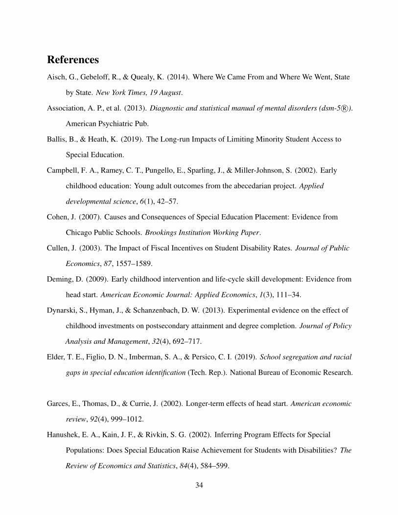
ReferencesAisch, G., Gebeloff, R., & Quealy, K. (2014). Where We Came From and Where We Went, State

by State. New York Times, 19 August.

Association, A. P., et al. (2013). Diagnostic and statistical manual of mental disorders (dsm-5 R�).

American Psychiatric Pub.

Ballis, B., & Heath, K. (2019). The Long-run Impacts of Limiting Minority Student Access to

Special Education.

Campbell, F. A., Ramey, C. T., Pungello, E., Sparling, J., & Miller-Johnson, S. (2002). Early

childhood education: Young adult outcomes from the abecedarian project. Applied

developmental science, 6(1), 42–57.

Cohen, J. (2007). Causes and Consequences of Special Education Placement: Evidence from

Chicago Public Schools. Brookings Institution Working Paper.

Cullen, J. (2003). The Impact of Fiscal Incentives on Student Disability Rates. Journal of Public

Economics, 87, 1557–1589.

Deming, D. (2009). Early childhood intervention and life-cycle skill development: Evidence from

head start. American Economic Journal: Applied Economics, 1(3), 111–34.

Dynarski, S., Hyman, J., & Schanzenbach, D. W. (2013). Experimental evidence on the effect of

childhood investments on postsecondary attainment and degree completion. Journal of Policy

Analysis and Management, 32(4), 692–717.

Elder, T. E., Figlio, D. N., Imberman, S. A., & Persico, C. I. (2019). School segregation and racial

gaps in special education identification (Tech. Rep.). National Bureau of Economic Research.

Garces, E., Thomas, D., & Currie, J. (2002). Longer-term effects of head start. American economic

review, 92(4), 999–1012.

Hanushek, E. A., Kain, J. F., & Rivkin, S. G. (2002). Inferring Program Effects for Special

Populations: Does Special Education Raise Achievement for Students with Disabilities? The

Review of Economics and Statistics, 84(4), 584–599.

34

Hibel, J., Farkas, G., & Morgan, P. (2010). Who is Placed into Special Education? Sociology of

Education, 83(4), 312–332.

Hill, I., et al. (2004). State responses to budget crises in 2004: Texas. Washington, DC: The Urban

Institute.

Jackson, C. K., Johnson, R. C., & Persico, C. (2015). The effects of school spending on

educational and economic outcomes: Evidence from school finance reforms. The Quarterly

Journal of Economics, 131(1), 157–218.

Kauffman, J. M., Hallahan, D. P., & Pullen, P. C. (2017). Handbook of special education.

Routledge.

KidsHealth. (2016). 504 Education Plans. Retrieved from

https://kidshealth.org/en/parents/504-plans.html

Koseki, M. H. (2017). Meeting the needs of all students: Amending the idea to support special

education students from low-income households. Fordham Urb. LJ, 44, 793.

Levin, H. M., Belfield, C., Muennig, P., & Rouse, C. (2007). The public returns to public

educational investments in african-american males. Economics of Education review, 26(6),

699–708.

National Center for Education Statistics. (2015). The Condition of Education At A Glance.

Retrieved from http://nces.ed.gov/programs/coe/indicator cgg.asp

Newman, L., Wagner, M., Knokey, A.-M., Marder, C., Nagle, K., Shaver, D., & Wei, X. (2011).

The Post-High School Outcomes of Young Adults with Disabilities up to 8 Years after High

School: A Report from the National Longitudinal Transition Study-2 (NLTS2). National

Center for Special Education Research, 2, 1–218.

Prenovitz, S. (2017). Accountability Incentives and Special Education.

Rosenthal, B. (2016). Denied: How Texas Keeps Tens of Thousands of Children Out of Special

Education. Houston Chronicle.

Schweinhart, L. J., Montie, J., Xiang, Z., Barnett, W. S., Belfield, C., & Nores, M. (2005). The

high/scope perry preschool study through age 40. Ypsilanti, MI: High Scope Educational

35

Research Foundation.

Setren, E. (2019). The Impact of Specialized Services vs. High Quality General Education on

Special Education and English Language Learner Students. Working Paper.

Texas Education Agency. (2016). 2016-2017 PBMAS Staging Framework.

Texas Education Agency. (2018). Secondary School Completion and Dropouts in Texas Public

Schools 2016-17. Retrieved from

https://tea.texas.gov/acctres/dropcomp index.html

White, S., Potter, L., You, H., Valencia, L., Jordan, J., & Pecotte, B. (2016). Introduction to Texas

Domestic Migration. Office of the State Demographer.

36

Figures/Tables

Figure 1: Change in District level SE enrollment during the pre-policy period (2000-2005) and thepost-policy period (2005-2010)

Note: This figure shows the change in SE enrollment between 2000-2005 and 2005-2010 by SE enrollment in 2004-05.The district level changes are weighted by 2004-05 district enrollment.

37

Figure 2: Event Study Estimates of the Impact of the Policy on SE Removal in Expected 9th Grade(High Impact Sample)

Note: This figure plots coefficients and 95% confidence intervals from an event-study regression that estimatesinteractions between 5th grade cohort dummies and the 2004-05 district SE rate. The outcome is an indicator for SEremoval, measured in the year each student was expected to be enrolled in 9th grade (or 4 years after 5th grade). Eventtime is computed by subtracting 9 from the grade each 5th grade cohort was expected to be enrolled in during thefirst year of the policy (or the 2005-06 school year). The sample includes 5th grade cohorts enrolled in SE between1995-96 to 2004-05 in our high impact sample, including students with a malleable disability (including learningdisabilities, speech impairments, other health impairments (includes ADHD), or emotional disturbance) who spentmore than 50 percent of their instruction in general education classrooms at baseline (measured as of 5th grade). The5th grade cohort from 1995-96 is omitted, so estimates are relative to that unexposed cohort. This regression includescontrols for 5th grade cohort indicators, district fixed effects, gender, race, FRL status, ELL classification, gender-raceinteractions, baseline primary disability, an indicator for whether a student took the unmodified version of the exam,level of classroom inclusion (all measured at baseline in 5th grade). This regression also includes controls for districtcontrols that include tax base wealth per-pupil and the percent of tax base wealth that is residential, as well as thepercentage of students in a district and cohort belonging to each racial group, receiving FRL, classified as ELL, andwho are male for the SE sample and the full sample. Standard errors are clustered by district.

38

Figure 3: Event Study Estimates of the Impact of the Policy on Educational Attainment (HighImpact Sample)

(a) High School Completion

(b) College Enrollment

Note: These figures plot coefficients and 95% confidence intervals from event-study regressions that estimatesinteractions between 5th grade cohort dummies and the 2004-05 district SE rate. The dependent variable is shown in thesub-figure labels. College enrollment is measured within four years of each student’s expected high school graduation.Event time is computed by subtracting 9 from the grade each 5th grade cohort was expected to be enrolled in during thefirst year of the policy (or the 2005-06 school year). The sample includes 5th grade cohorts enrolled in SE between1996-97 to 2004-05 who were in our high impact sample. The 5th grade cohort from 1996-97 is omitted, so estimatesare relative to that unexposed cohort. See Figure 2 for more detail on the sample and the full set of controls. Standarderrors are clustered by district.

39

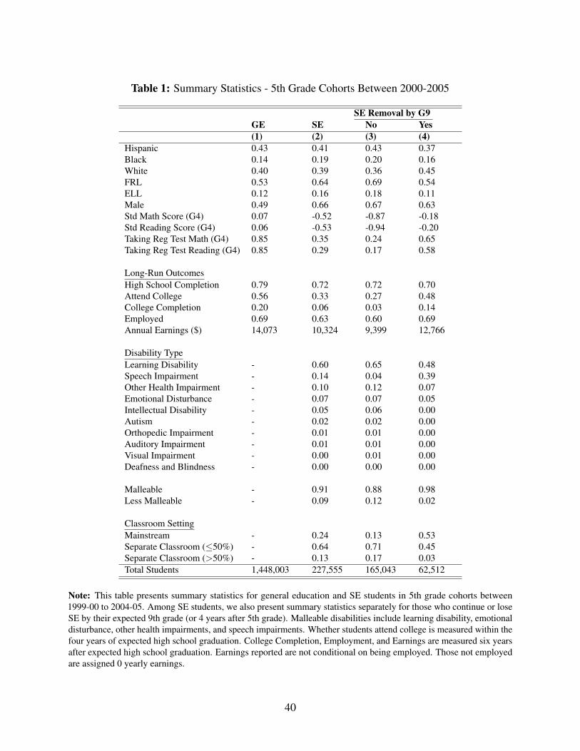
Table 1: Summary Statistics - 5th Grade Cohorts Between 2000-2005

SE Removal by G9GE SE No Yes(1) (2) (3) (4)

Hispanic 0.43 0.41 0.43 0.37Black 0.14 0.19 0.20 0.16White 0.40 0.39 0.36 0.45FRL 0.53 0.64 0.69 0.54ELL 0.12 0.16 0.18 0.11Male 0.49 0.66 0.67 0.63Std Math Score (G4) 0.07 -0.52 -0.87 -0.18Std Reading Score (G4) 0.06 -0.53 -0.94 -0.20Taking Reg Test Math (G4) 0.85 0.35 0.24 0.65Taking Reg Test Reading (G4) 0.85 0.29 0.17 0.58

Long-Run OutcomesHigh School Completion 0.79 0.72 0.72 0.70Attend College 0.56 0.33 0.27 0.48College Completion 0.20 0.06 0.03 0.14Employed 0.69 0.63 0.60 0.69Annual Earnings ($) 14,073 10,324 9,399 12,766

Disability TypeLearning Disability - 0.60 0.65 0.48Speech Impairment - 0.14 0.04 0.39Other Health Impairment - 0.10 0.12 0.07Emotional Disturbance - 0.07 0.07 0.05Intellectual Disability - 0.05 0.06 0.00Autism - 0.02 0.02 0.00Orthopedic Impairment - 0.01 0.01 0.00Auditory Impairment - 0.01 0.01 0.00Visual Impairment - 0.00 0.01 0.00Deafness and Blindness - 0.00 0.00 0.00

Malleable - 0.91 0.88 0.98Less Malleable - 0.09 0.12 0.02

Classroom SettingMainstream - 0.24 0.13 0.53Separate Classroom (50%) - 0.64 0.71 0.45Separate Classroom (>50%) - 0.13 0.17 0.03Total Students 1,448,003 227,555 165,043 62,512

Note: This table presents summary statistics for general education and SE students in 5th grade cohorts between1999-00 to 2004-05. Among SE students, we also present summary statistics separately for those who continue or loseSE by their expected 9th grade (or 4 years after 5th grade). Malleable disabilities include learning disability, emotionaldisturbance, other health impairments, and speech impairments. Whether students attend college is measured within thefour years of expected high school graduation. College Completion, Employment, and Earnings are measured six yearsafter expected high school graduation. Earnings reported are not conditional on being employed. Those not employedare assigned 0 yearly earnings.

40

Table 2: The Impact of the Policy on SE Removal in Expected 9th Grade

(1) (2) (3) (4) (5)

Panel A: Full SampleTreatment 0.0102*** 0.00955*** 0.00816*** 0.00788*** 0.00778***

(0.00206) (0.00210) (0.00214) (0.00188) (0.00188)[0.048] [0.043] [0.037] [0.035] [0.035]

Mean (Y) 0.275 0.275 0.275 0.275 0.275N 227,555 227,555 227,555 227,555 227,555

Panel B: High Impact SampleTreatment 0.0108*** 0.0100*** 0.00961*** 0.00931*** 0.00921***

(0.00277) (0.00279) (0.00235) (0.00213) (0.00213)[0.049] [0.045] [0.043] [0.042] [0.042]

Mean (Y) 0.317 0.317 0.317 0.317 0.317N 189,042 189,042 189,042 189,042 189,042

ControlsCohort FE X X X X XDistrict FE X X X X XIndividual Demo X X X XIndividual Disability X X XDistrict-Cohort Demo X XDistrict Finance X

Note: This table shows difference-in-differences estimates of the impact of the policy on SE removal. Within eachpanel, each column reports estimates of d1 from a separate regression of Equation 2. The outcome variable is anindicator for whether a student lost SE services the year they were expected to be enrolled in 9th grade (or four yearsafter 5th grade). The sample includes 5th grade cohorts enrolled in SE between 1999-00 to 2004-05. Panel A includesestimates for the full sample. Panel B includes estimates for our high impact sample that include students with amalleable disability (including learning disabilities, speech impairments, other health impairments (includes ADHD),or emotional disturbance) who received more than 50 percent of their instruction in general education classrooms atbaseline (both measured as of 5th grade). Individual controls include gender, race, FRL status, ELL classification,gender-race interactions, baseline primary disability, an indicator for whether a student took the unmodified version ofthe exam, and baseline level of classroom inclusion (all measured in 5th grade). District demographic cohort controlsinclude the percentage of students belonging to each racial group, receiving FRL, classified as ELL, and who are malefor the SE sample and the full sample measured at baseline. District financial controls include tax base wealth per-pupiland the percent of tax base wealth that is residential. The effect for the fully exposed student at the average district areshown in brackets, and is defined as the coefficient multiplied by 4.5. Standard errors in parentheses are clustered bydistrict. *p<0.10, ** p<0.05, *** p<0.01.

41

Table 3: The Impact of the Policy on Educational Attainment

(1) (2) (3) (4) (5)High School CompletionPanel A: Full SampleTreatment -0.00409*** -0.00455*** -0.00427*** -0.00428*** -0.00421***

(0.00142) (0.00141) (0.00147) (0.00141) (0.00142)[-0.018] [-0.020] [-0.019] [-0.019] [-0.019]

Mean (Y) 0.718 0.718 0.718 0.718 0.718N 227,555 227,555 227,555 227,555 227,555

Panel B: High Impact SampleTreatment -0.00466*** -0.00515*** -0.00523*** -0.00510*** -0.00497***

(0.00156) (0.00156) (0.00161) (0.00156) (0.00157)[-0.021] [-0.023] [-0.024] [-0.023] [-0.022]

Mean (Y) 0.710 0.710 0.710 0.710 0.710N 189,042 189,042 189,042 189,042 189,042

College EnrollmentPanel C: Full SampleTreatment -0.00118 -0.00214* -0.00223 -0.00266** -0.00264**

(0.00131) (0.00129) (0.00136) (0.00134) (0.00134)[-0.005] [-0.010] [-0.010] [-0.012] [-0.012]

Mean (Y) 0.327 0.327 0.327 0.327 0.327N 227,555 227,555 227,555 227,555 227,555

Panel D: High Impact SampleTreatment -0.00281* -0.00377*** -0.00340** -0.00376** -0.00372**

(0.00143) (0.00140) (0.00148) (0.00149) (0.00149)[-0.013] [-0.017] [-0.015] [-0.017] [-0.017]

Mean (Y) 0.354 0.354 0.354 0.354 0.354N 189,042 189,042 189,042 189,042 189,042

ControlsCohort & District FE X X X X XIndividual Demo X X X XIndividual Disability X X XDistrict-Cohort Demo X XDistrict Finance X

Note: This table shows difference-in-differences estimates of the impact of the policy on educational attainmentdecisions. Within each panel, each column reports estimates of d1 from a separate regression of Equation 2. Thedependent variable is shown in bold. College enrollment is measured within four years of each student’s expected highschool graduation. Panels A and C include estimates for the full sample. Panels B and D include estimates for the highimpact sample. The sample includes 5th grade cohorts enrolled in SE between 1999-00 to 2004-05. See Table 2 formore detail on the sample and the full set of controls. The effect for the fully exposed student at the average district areshown in brackets, and is defined as the coefficient multiplied by 4.5. Standard errors in parentheses are clustered bydistrict. *p<0.10, ** p<0.05, *** p<0.01.

42

Table 4: OLS and IV Estimates of the Impact of SE Removal on Educational Attainment (HighImpact Sample)

FS RF OLS IV(1) (2) (3) (4)

Dependent Variable: SE Removal - High School CompletionG9 (Expected)

Treatment 0.00921*** -0.00497***(0.00157) (0.00213)[0.0414] [-0.022]

Mean (Y) 0.317 0.710

SE Removal -0.0800*** -0.522***(0.00213) (0.184)

Dependent Variable: SE Removal -G9 (Expected) College Enrollment

Treatment 0.00921*** -0.00372**(0.00157) (0.00149)[0.0414] [-0.017]

Mean (Y) 0.317 0.354

SE Removal 0.0717*** -0.378**(0.00361) (0.187)

Kleibergen-PaapF-Statisitic 17.02

Notes: This table reports difference-in-differences estimates of the impact of the policy on SE removal (by expected9th grade) and educational attainment (Columns 1 -2). This table also reports OLS and IV estimates of SE removalon educational attainment outcomes (Columns 3-4). The dependent variable is shown in the panel headings. Collegeenrollment is measured within four years of each student’s expected high school graduation. The sample includes 5thgrade cohorts enrolled in SE between 1999-00 to 2004-05 in our high impact sample (N=189,042). See Table 2 formore detail on the sample and for the full list of controls used. The effect for the fully exposed student at the averagedistrict are shown in brackets, and is defined as the coefficient multiplied by 4.5. Standard errors in parentheses areclustered by district. *p< 0.10, **p < 0.05, *** p< 0.01.

43

Table 5: Heterogeneity by Race and FRL Status (High Impact Sample)

FRL Non-FRL Minority White(1) (2) (3) (4)

Panel A: SE Removal in G9 (Expected)Treatment 0.0114*** 0.0053 0.0108*** 0.0063**

(0.0023) (0.0030) (0.0028) (0.0024)P-value 0.026 0.256

Mean (Y) 0.265 0.409 0.281 0.367Panel B: High School Completion

Difference-in-Differences EstimatesTreatment -0.0056** -0.0050** -0.0063** -0.0030

(0.0021) (0.0019) (0.0023) (0.0018)P-value 0.820 0.172

IV EstimatesSE Removal -0.49531** -0.9568 - 0.57848* -0.4083

(0.1867) (0.6065) (0.2436) (0.3179)P-value 0.506 0.000

Mean (Y) 0.653 0.811 0.678 0.756Panel C: College Enrollment

Difference-in-Differences EstimatesTreatment -0.00566*** -0.0006 -0.00742*** 0.0007

(0.002) (0.003) (0.002) (0.002)P-value 0.060 0.000

IV EstimatesSE Removal -0.49879** -0.1074 -0.68757* 0.1101

(0.1777) (0.5426) (0.2809) (0.3056)P-value 0.000 0.000

Mean (Y) 0.268 0.506 0.313 0.410

N 120,565 68,429 112,462 73,959KP F-statistic 23.7527 3.0476 14.8290 6.8305

Notes: Panel A reports difference-in-differences estimates of the impact of the policy on SE removal. Panel B reportsdifference-in-differences estimates of the impact of the policy on high school completion and IV estimates of SEremoval on high school completion. Panel C reports difference-in-differences estimates of the impact of the policyon college enrollment and IV estimates of SE removal on college enrollment. College enrollment is measured withinfour years of each student’s expected high school graduation. The sample includes 5th grade cohorts enrolled in SEbetween 1999-00 to 2004-05 in our high impact sample. See Table 2 for more detail on the sample and for the full listof controls used. The p-value row presents the p-value associated with the test of equality across the two coefficients(either Columns 1 vs. 2 or Columns 3 vs. 4). Standard errors in parentheses are clustered by district. *p< 0.10, **p< 0.05, *** p< 0.01. 44

Tabl

e6:

The

Impa

ctof

the

Polic

yon

Inte

rmed

iate

Out

com

es

Shar

eR

epea

ted

Std

Scor

eTo

okH

SEx

itU

nabl

eto

Pass

HS

Exit

Abs

ent

Gra

de9

Mat

hR

eadi

ngM

ath

Rea

ding

Mat

hR

eadi

ng

(1)

(2)

(3)

(4)

(5)

(6)

(7)

(8)

Pane

lA:F

ullS

ampl

eTr

eatm

ent

0.00

010.

0004

0.00

140.

0098

*0.

0059

***

0.00

48**

0.00

38**

*0.

0013

**(0

.000

2)(0

.000

5)(0

.004

9)(0

.005

2)(0

.002

0)(0

.002

0)(0

.001

0)(0

.000

6)[0

.00]

[0.0

0][0

.01]

[0.0

4][0

.03]

[0.0

2][0

.02]

[0.0

1]M

ean

(Y)

0.06

90.

026

-0.4

44-0

.545

0.31

40.

324

0.10

00.

044

N22

7,55

522

7,55

599

,029

102,

346

227,

555

227,

555

227,

555

227,

555

Pane

lB:H

igh

Impa

ctSa

mpl

eTr

eatm

ent

8.62

e-05

-6.7

8e-0

5-0

.000

929

0.00

713

0.00

628*

**0.

0052

5**

0.00

454*

**0.

0016

4**

(0.0

003)

(0.0

004)

(0.0

048)

(0.0

052)

(0.0

022)

(0.0

022)

(0.0

012)

(0.0

007)

..

[-0.

00]

[0.0

3][0

.03]

[0.0

2][0

.02]

[0.0

1]M

ean

(Y)

0.06

90.

020

-0.4

37-0

.530

0.35

50.

366

0.11

10.

048

N18

9,04

218

9,04

292

,753

95,4

3018

9,04

218

9,04

218

9,04

218

9,04

2

Not

e:Th

ista

ble

show

sdi

ffer

ence

-in-d

iffer

ence

ses

timat

esof

the

impa

ctof

the

polic

yon

inte

rmed

iate

outc

omes

.With

inea

chpa

nel,

each

colu

mn

repo

rtses

timat

esof

d 1fr

oma

sepa

rate

regr

essi

onof

Equa

tion

2.Th

ede

pend

entv

aria

ble

issh

own

inth

eco

lum

nhe

adin

gs.T

heou

tcom

esin

colu

mns

1th

roug

h4

are

mea

sure

din

expe

cted

9th

grad

e.Th

eou

tcom

esin

Col

umns

6th

roug

h8

are

are

mea

sure

din

expe

cted

10th

grad

e.Pa

nelA

estim

ates

fort

hefu

llsa

mpl

e.Pa

nelB

estim

ates

from

ourh

igh

impa

ctsa

mpl

e.Th

esa

mpl

ein

clud

es5t

hgr

ade

coho

rtsen

rolle

din

SEbe

twee

n19

99-0

0to

2004

-05.

See

Tabl

e2

form

ore

deta

ilon

the

sam

ple

and

the

full

set

ofco

ntro

ls.T

heef

fect

fort

hefu

llyex

pose

dst

uden

tatt

heav

erag

edi

stric

tare

show

nin

brac

kets

,and

isde

fined

asth

eco

effic

ient

mul

tiplie

dby

4.5.

Stan

dard

erro

rsin

pare

nthe

ses

are

clus

tere

dby

dist

rict.

*p<

0.10

,**

p<0.

05,*

**p<

0.01

.

45

Tabl

e7:

Het

erog

enei

tyby

Scho

ol-B

ased

Fact

ors

(Hig

hIm

pact

Sam

ple)

(1)

(2)

(3)

(4)

(5)

(6)

(7)

(8)

(9)

Dis

trict

Wea

lth50

4Pl

anG

row

th.

Ave

rage

Test

Scor

esD

istri

ctVa

lue

Add

edB

asel

ine

Hig

hLo

wH

igh

Low

Hig

hLo

wH

igh

Low

Pane

lA:S

ERe

mov

alin

G9

(Exp

ecte

d)Tr

eatm

ent

0.00

836*

**0.

0165

**0.

0082

9***

0.01

56**

*0.

0067

6***

0.00

601*

*0.

0107

***

0.01

11**

*0.

0072

5**

(0.0

0214

)(0

.006

32)

(0.0

0225

)(0

.004

60)

(0.0

0254

)(0

.002

64)

(0.0

0282

)(0

.003

10)

(0.0

0327

)[0

.04]

[0.0

7][0

.04]

[0.0

7][0

.03]

[0.0

3][0

.05]

[0.0

5][0

.03]

Mea

n(Y

)0.

317

0.36

90.

315

0.28

40.

326

0.36

30.

289

0.33

20.

308

Pane

lB:H

igh

Scho

olC

ompl

etio

nTr

eatm

ent

-0.0

0509

***

-0.0

0580

-0.0

0517

***

-0.0

0147

-0.0

0569

***

-0.0

0358

-0.0

0585

***

-0.0

0366

-0.0

0591

***

(0.0

0157

)(0

.006

12)

(0.0

0163

)(0

.002

96)

(0.0

0183

)(0

.002

19)

(0.0

0205

)(0

.002

40)

(0.0

0215

)[-

0.02

][-

0.03

][-

0.02

][-

0.01

][-

0.03

][-

0.02

][-

0.03

][-

0.02

][-

0.03

]M

ean

(Y)

0.71

00.

793

0.70

60.

712

0.71

00.

756

0.68

20.

746

0.68

7

Pane

lC:C

olle

geEn

rollm

ent

Trea

tmen

t-0

.004

44**

*-0

.004

07-0

.004

59**

*-0

.003

88-0

.004

36**

-0.0

0201

-0.0

0629

***

-0.0

0175

-0.0

0605

***

(0.0

0157

)(0

.003

66)

(0.0

0160

)(0

.002

90)

(0.0

0192

)(0

.002

91)

(0.0

0173

)(0

.002

00)

(0.0

0227

)[-

0.02

][-

0.02

][-

0.02

][-

0.02

][-

0.02

][-

0.01

][-

0.03

][-

0.01

][-

0.03

]M

ean

(Y)

0.35

40.

452

0.34

90.

330

0.36

00.

419

0.31

40.

390

0.33

1

N18

9,04

29,

810

179,

232

37,5

6115

1,48

172

,317

116,

725

73,5

9811

5,44

4

Not

e:Th

ista

ble

show

sdi

ffer

ence

-in-d

iffer

ence

ses

timat

esof

the

impa

ctof

the

polic

yon

SEre

mov

alan

ded

ucat

iona

latta

inm

entd

ecis

ions

ford

iffer

entt

ype

ofdi

stric

ts.H

igh

wea

lthdi

stric

tsha

dta

xba

sew

ealth

per-

pupi

lgre

ater

than

$323

(inth

ousa

nds

ofdo

llars

)and

mad

eup

the

top

12%

ofsc

hool

dist

ricts

inte

rms

ofta

x-ba

sew

ealth

.We

cons

truct

valu

e-ad

ded

asfo

llow

s.W

ere

gres

sav

erag

est

anda

rdiz

edte

stsc

ores

onla

gged

test

scor

es,i

ndic

ator

sfo

rast

uden

t’sra

ce,g

ende

r,SE

stat

us,L

imite

dEn

glis

hPr

ofici

ency

stat

us,a

ndFr

eean

dR

educ

edPr

ice

Lunc

hst

atus

.We

split

dist

ricts

acco

rdin

gto

the

med

ian

ofea

chsc

hool

-bas

edm

easu

re,w

here

thos

eab

ove

the

med

ian

are

labe

lled

“Hig

h”an

dth

ose

belo

war

ela

belle

d“L

ow”.

With

inea

chpa

nel,

each

colu

mn

repo

rtses

timat

esof

d 1fr

oma

sepa

rate

regr

essi

onof

Equa

tion

2.Th

ede

pend

entv

aria

ble

issh

own

inth

epa

nelh

eadi

ngs.

This

tabl

ein

clud

eses

timat

esfr

omou

rhig

him

pact

sam

ple.

The

sam

ple

incl

udes

5th

grad

eco

horts

enro

lled

inSE

betw

een

1999

-00

to20

04-0

5.Se

eTa

ble

2fo

rmor

ede

tail

onth

esa

mpl

ean

dth

efu

llse

tofc

ontro

ls.T

heef

fect

fort

hefu

llyex

pose

dst

uden

tat

the

aver

age

dist

ricta

resh

own

inbr

acke

ts,a

ndis

defin

edas

the

coef

ficie

ntm

ultip

lied

by4.

5.St

anda

rder

rors

inpa

rent

hese

sar

ecl

uste

red

bydi

stric

t.*p

<0.

10,*

*p<

0.05

,***

p<0.

01.

46

A Appendix

Figure A.1: Transition Plan College Bound Student – Page 1

47

Figure A.2: Transition Plan College Bound Student – Page 2

48

Figure A.3: Performance Level Assignment for the SE Representation Rate Indicator

Note: State Interventions increased in severity with distance from 8.5, ranging from designing and implementing animprovement plan with school districts to state audits. Source: PBMAS 2004-05

Figure A.4: Entrance and Exit Rates for students with Malleable Disabilities

Note: The figure plots entrance rates (solid line) and exit rates (dashed line) in each grade for students with malleabledisabilities. Entrance rates represent the number of new students enrolled in SE, divided by the total number of studentsenrolled in the current grade. Exit rates represent the number of students who lost SE, divided by the total number ofstudents enrolled in SE during the grade prior. The sample includes cohorts who were completely unexposed to thepolicy.

49

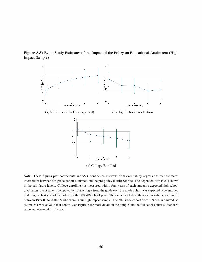
Figure A.5: Event Study Estimates of the Impact of the Policy on Educational Attainment (HighImpact Sample)

(a) SE Removal in G9 (Expected) (b) High School Graduation

(c) College Enrolled

Note: These figures plot coefficients and 95% confidence intervals from event-study regressions that estimatesinteractions between 5th grade cohort dummies and the pre-policy district SE rate. The dependent variable is shownin the sub-figure labels. College enrollment is measured within four years of each student’s expected high schoolgraduation. Event time is computed by subtracting 9 from the grade each 5th grade cohort was expected to be enrolledin during the first year of the policy (or the 2005-06 school year). The sample includes 5th grade cohorts enrolled in SEbetween 1999-00 to 2004-05 who were in our high impact sample. The 5th Grade cohort from 1999-00 is omitted, soestimates are relative to that cohort. See Figure 2 for more detail on the sample and the full set of controls. Standarderrors are clustered by district.

50

Figure A.6: Event Study Estimates of the Impact of the Policy on SE Removal Any Time after 5thGrade (High Impact Sample)

Note: These figures plot coefficients and 95% confidence intervals from event-study regressions that estimatesinteractions between 5th grade cohort dummies and the pre-policy district SE rate. The dependent variable is anindicator variable for whether a student ever lost SE services after 5th grade. Event time is defined as the grade each 5thgrade cohort was expected to be enrolled in during the first year of the policy (or the 2005-06 school year). The sampleincludes 5th grade cohorts enrolled in SE between 1995-96 to 2004-05 who were in our high impact sample. The 5thGrade cohort from 1995-96 is omitted, so estimates are relative to that unexposedcohort. See Figure 2 for more detailon the sample and the full set of controls. Standard errors are clustered by district.

51

Figure A.7: Earnings Trajectories by College Enrollment Choice

Note: This figure plots the earnings trajectories 13 years after expected high school graduation based on an individuals’decision to enroll in college within four years of each student’s expected high school graduation. The sample includesstudents who were in the 1999-00 5th grade SE cohort.

Figure A.8: State Level Participation in 504 Plans and SE Programs

Note: Data for this figure come from the IES. Averages represent district level population averages, that is, the numberof students in special education (or 504 plans), divided by the total number of students in that district and year.

52

Table A.1: Policy Pressure due to PBMAS (2004-05 School Year)

Panel A: Fraction of Districts meeting standards in each PBMAS Monitoring CategoryReduce Services

PBMAS Reduce SE Enrollment Improve Outcomes Separate ModifiedPerformance Level Overall Black Hispanic Behavioral Academic Instruction Test-Taking

(1) (2) (3) (4) (5) (6) (7)0 = Met 0.05 0.53 0.67 0.72 0.97 0.39 0.241 = Nearly Met 0.19 0.08 0.07 0.27 0.03 0.38 0.652 = Not Met 0.53 0.13 0.10 0.02 0.00 0.19 0.113 = Worst Rating 0.24 0.19 0.12 0.00 0.00 0.03 0.00

Panel B: Correlation b/w Pressure to Reduce Overall SE Enrollment and other PBMAS PressuresReduce Services

Reduce SE Enrollment Improve Outcomes Separate ModifiedBlack Hispanic Behavioral Academic Instruction Test-Taking

(2) (3) (4) (5) (6) (7)Correlation Coefficient 0.0122 0.0428 -0.0954* 0.0025 0.0604 0.0976*

Note: This table shows the policy pressure to make changes for SE due to the introduction of PBMAS Monitoring in2005. Panel A shows the fraction of districts that met (0), nearly met standards (1), did not meet (2), or had the worstrating (3) under each area of SE monitoring during 2005. Panel B shows the raw correlation coefficient between thepolicy pressure to reduce overall SE enrollment (based on the distance above the 8.5 SE enrollment target get in 2005)and the average rating in each of the other PBMAS monitoring areas (measured in 2005). *p< 0.10, **p < 0.05, ***p< 0.01

53

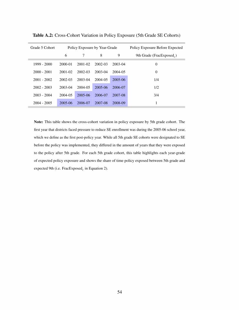
Table A.2: Cross-Cohort Variation in Policy Exposure (5th Grade SE Cohorts)

Grade 5 Cohort Policy Exposure by Year-Grade Policy Exposure Before Expected

6 7 8 9 9th Grade (FracExposedc)

1999 - 2000 2000-01 2001-02 2002-03 2003-04 0

2000 - 2001 2001-02 2002-03 2003-04 2004-05 0

2001 - 2002 2002-03 2003-04 2004-05 2005-06 1/4

2002 - 2003 2003-04 2004-05 2005-06 2006-07 1/2

2003 - 2004 2004-05 2005-06 2006-07 2007-08 3/4

2004 - 2005 2005-06 2006-07 2007-08 2008-09 1

Note: This table shows the cross-cohort variation in policy exposure by 5th grade cohort. The

first year that districts faced pressure to reduce SE enrollment was during the 2005-06 school year,

which we define as the first post-policy year. While all 5th grade SE cohorts were designated to SE

before the policy was implemented, they differed in the amount of years that they were exposed

to the policy after 5th grade. For each 5th grade cohort, this table highlights each year-grade

of expected policy exposure and shows the share of time policy exposed between 5th grade and

expected 9th (i.e. FracExposedc in Equation 2).

54

Table A.3: The Impact of the Policy on Attrition, Predicted Long-Run Outcomes, and ExogenousStudent Characteristics

PredictedDistrict SE

Enrollment Switch Removal High School College(By G9) (By G9) (By G9) Completion Enrollment Hispanic White FRL

(1) (2) (3) (4) (5) (6) (7) (8)Panel A: Full SampleTreatment -0.0003 0.0002 0.0030** 3.00e-05 0.0012** -0.0016 0.0020 -0.0015

(0.0007) (0.0010) (0.0012) (0.0003) (0.0005) (0.0011) (0.0012) (0.0014)[-.001] [.001] [0.01] [0.00] [0.01] [-0.01] [0.01] [-0.01]

Mean 0.902 0.235 0.275 0.718 0.332 0.412 0.386 0.644N 252,315 227,555 227,555 227,555 227,555 227,555 227,555 227,555

Panel B: High Impact SampleTreatment -0.0007 0.0006 0.0024 0.0004* 0.0009 0.0004 -0.0004 0.0004

(0.0008) (0.0011) (0.0015) (0.0002) (0.0006) (0.0003) (0.0003) (0.0003)[-.003] [.003] [0.01] [0.00] [0.00] [0.00] [-0.00] [0.00]

Mean 0.905 0.234 0.317 0.710 0.359 0.421 0.391 0.638N 208,944 189,042 189,042 189,042 189,042 189,042 189,042 189,042

ControlsFE’s X X X X X X X XCohort Demo X X X X X X X XAddt’l Controls X X

Note: This table shows difference-in-differences estimates of the impact of the policy on attrition (by expected 9thgrade), predicted outcomes, and student demographic characteristics. Within each panel, each column reports estimatesof d1 from a separate regression of Equation 2. The dependent variable is shown in the column headings. To obtainpredicted values we generate fitted values from a regression of outcomes on the full set of controls (excluding treatment).Panel A include estimates for the full sample and Panel B include estimates from our high impact sample. The sampleincludes 5th grade cohorts enrolled in SE between 1999-00 to 2004-05. See Table 2 for more detail on the sampleand the full set of controls. The effect for the fully exposed student at the average district are shown in brackets, andis defined as the coefficient multiplied by 4.5. Standard errors in parentheses are clustered by district. *p<0.10, **p<0.05, *** p<0.01.

55

Table A.4: The Effect of the Enrollment Target on SE Placement and Education Attainment–Accounting for Differences in District Level Demographics (High Impact Sample)

(1) (2) (3) (4)

Panel A: Likelihood of Losing SE, 4 Years after G5Treatment 0.00836*** 0.00775*** 0.00799*** 0.00818***

(0.00214) (0.00239) (0.00266) (0.00214)[0.038] [0.035] [0.036] [0.037]

Mean (Y) 0.317 0.317 . 0.317 0.317

Panel B: Likelihood of Graduating from High SchoolTreatment -0.00509*** -0.00373** -0.00442*** -0.00465***

(0.00157) (0.00155) (0.00170) (0.00145)[-0.023] [-0.017] [-0.020] [-0.021]

Mean (Y) 0.710 0.710 0.710 0.710

Panel C: Likelihood of Enrolling in CollegeTreatment -0.00444*** -0.00401** -0.00455** -0.00412***

(0.00157) (0.00167) (0.00190) (0.00147)[-0.020] [-0.018] [-0.020] [-0.019]

Mean (Y) 0.354 0.354 0.354 0.354

ControlsFull Set X X X Xf (t)⇥ Fraction Hispanic Xf (t)⇥ Cohort Size Xf (t)⇥ Fraction FRL X

Note: This table shows difference-in-differences estimates of the impact of the policy on the likelihood of SE removaland educational attainment decisions. Within each panel, Within each panel, each column reports estimates of d1 froma separate regression of Equation 2. The dependent variable is shown in the panel headings. The sample includes 5thgrade cohorts enrolled in SE between 1999-00 to 2004-05 in our high impact sample. See Table 2 for more detail onthe sample and the full set of controls. We also include linear time trends that vary by the fraction of the district thatwas Hispanic, and FRL in 2004-05, as well as a linear trend for the total cohort size in 2004-05. The effect for thefully exposed student at the average district are shown in brackets, and is defined as the coefficient multiplied by 4.5.Standard errors in parentheses are clustered by district. *p<0.10, ** p<0.05, *** p<0.01.

56

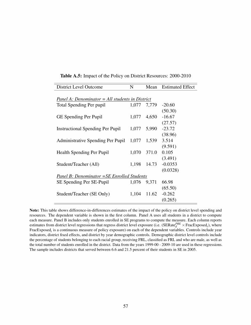
Table A.5: Impact of the Policy on District Resources: 2000-2010

District Level Outcome N Mean Estimated Effect

Panel A: Denominator = All students in DistrictTotal Spending Per pupil 1,077 7,779 -20.60

(50.30)GE Spending Per Pupil 1,077 4,650 -16.67

(27.57)Instructional Spending Per Pupil 1,077 5,990 -23.72

(38.96)Administrative Spending Per Pupil 1,077 1,539 3.514

(9.591)Health Spending Per Pupil 1,070 371.0 0.105

(3.491)Student/Teacher (All) 1,198 14.73 -0.0353

(0.0328)Panel B: Denominator =SE Enrolled StudentsSE Spending Per SE-Pupil 1,076 9,371 66.98

(65.50)Student/Teacher (SE Only) 1,104 11.62 -0.262

(0.265)

Note: This table shows difference-in-differences estimates of the impact of the policy on district level spending andresources. The dependent variable is shown in the first column. Panel A uses all students in a district to computeeach measure. Panel B includes only students enrolled in SE programs to compute the measure. Each column reportsestimates from district level regressions that regress district level exposure (i.e. (SERatePRE

d ⇥FracExposedt), whereFracExposedt is a continuous measure of policy exposure) on each of the dependent variables. Controls include yearindicators, district fixed effects, and district by year demographic controls. Demographic district level controls includethe percentage of students belonging to each racial group, receiving FRL, classified as FRL and who are male, as well asthe total number of students enrolled in the district. Data from the years 1999-00 - 2009-10 are used in these regressions.The sample includes districts that served between 6.6 and 21.5 percent of their students in SE in 2005.

57

Table A.6: The Impact of Policy on Types of Services/Accommodations

RegularClassroom Unmodified Exam Ever

SE Removal (� 79 % day) Math Reading Disciplined(1) (2) (3) (4) (5)

Panel A: Full SampleTreatment 0.00688*** 0.00455 0.00685** 0.00484 -0.00175

(0.00189) (0.00316) (0.00313) (0.00323) (0.00154)[0.03] [0.02] [0.03] [0.02] [-0.01]

Mean (Y) 0.725 0.670 0.435 0.450 0.405N 227,555 227,555 227,555 227,555 227,555

Panel B: High Impact SampleTreatment 0.00836*** 0.00502 0.00778** 0.00557 -0.00175

(0.00214) (0.00311) (0.00342) (0.00354) (0.00158)[0.04] [0.02] [0.04] [0.03] [-0.01]

Mean (Y) 0.317 0.747 0.491 0.505 0.419N 189,042 189,042 189,042 189,042 189,042

ControlsFull Set X X X X X

Note: This table shows difference-in-differences estimates of the impact of the policy on intermediate outcomes. Withineach panel, each column reports estimates of d1 from a separate regression of Equation 2. The dependent variable isshown in the column headings. We identify a student as ever being disciplined in that year if the student had an inschool or out of school suspension, expulsions, or other disciplinary action. All dependent variables are measured in theyear each student was expected to be in 9th grade. Panel A estimates for the full sample. Panel B estimates from ourhigh impact sample. The sample includes 5th grade cohorts enrolled in SE between 1999-00 to 2004-05. See Table 2for more detail on the sample and the full set of controls. The effect for the fully exposed student at the average districtare shown in brackets, and is defined as the coefficient multiplied by 4.5. Standard errors in parentheses are clustered bydistrict. *p<0.10, ** p<0.05, *** p<0.01.

58

Table A.7: The Effect of the SE Enrollment Target on SE Removal and Educational Attainment(Low Impact Samples)

SE Removal High School Completion College Enrollment

Panel A: Severe Malleable DisabilitiesTreatment 0.00145 0.00127 -0.00397 -0.00732* -0.000293 -0.000766

(0.00398) (0.00320) (0.00455) (0.00423) (0.00405) (0.00380)[0.007] [0.006] [-0.018] [-0.033] [-0.001] [-0.003]

Mean (Y) 0.085 0.085 0.653 0.653 0.180 0.180N 17,280 17,280 17,280 17,280 17,280 17,280

Panel B: Non-Malleable DisabilitiesTreatment 0.000718 -0.000364 0.00325 0.000720 0.00155 -0.00182

(0.00259) (0.00240) (0.00263) (0.00282) (0.00402) (0.00333)[0.003] [-0.002] [0.015] [0.003] [0.007] [-0.008]

Mean (Y) 0.049 0.049 0.840 0.840 0.207 0.207N 21,233 21,233 21,233 21,233 21,233 21,233

ControlsYear FE X X X X X XDistrict FE X X X X X XAdditional Controls X X X

Note: This table shows difference-in-differences estimates of the impact of the policy on SE removal and educationalattainment. Within each panel, each column reports estimates of d1 from a separate regression of Equation 2. Thedependent variable is shown in the column headings. We identify a student as ever being disciplined in that yearif the student had an in school or out of school suspension, expulsions, or other disciplinary action. All dependentvariables are measured in the year each student was expected to be in 9th grade. Panel A includes students who werereceiving SE services in 5th grade who had malleable disabilities and spent the majority of the school day receivinginstruction in separate classrooms. Panel B only includes students who were receiving SE services in 5th grade whohad non-malleable disabilities. The sample includes 5th grade cohorts enrolled in SE between 1999-00 to 2004-05. SeeTable 2 for more detail on the sample and the full set of controls. The effect for the fully exposed student at the averagedistrict are shown in brackets, and is defined as the coefficient multiplied by 4.5. Standard errors in parentheses areclustered by district. *p<0.10, ** p<0.05, *** p<0.01.

59

Table A.8: The Effect of the SE Enrollment Target on College Completion and Labor MarketOutcomes – 6 Years after Expected High School Graduation

College Completion Positive Earnings Earnings

Panel A: Full SampleTreatment 0.000683 1.22e-05 -0.000939 -0.00170 -25.89 -20.75

(0.000543) (0.000537) (0.00185) (0.00139) (60.46) (49.21)[0.003] [0.000] [-0.004] [-0.008] [-116.505] [-93.375]

Mean(Y) 0.0627 0.0627 0.629 0.629 11335 11335N 227,555 227,555 227,555 227,555 227,555 227,555

Panel B: High Impact SampleTreatment 7.29e-05 -0.000503 -0.000953 -0.000904 -52.66 -28.39

(0.000651) (0.000629) (0.00156) (0.00147) (61.76) (58.16)[0.000] [-0.002] [-0.004] [-0.004] [-236.970] [-127.755]

Mean (Y) 0.0689 0.0689 0.674 0.674 12525 12525N 189,042 189,042 189,042 189,042 189,042 189,042

ControlsYear FE X X X X X XDistrict FE X X X X X XAdditional Controls X X X

Note: This table shows difference-in-differences estimates of the impact of the policy on college completion (i.e.earning a BA or a MA), being employed, and yearly earnings. These outcomes are all measured in the 6th year after astudent’s expected high school graduation. Within each panel, each column reports estimates of d1 from a separateregression of Equation 2. The dependent variable is shown in the column headings. Panel A estimates for the fullsample. Panel B estimates from our high impact sample. The sample includes 5th grade cohorts enrolled in SE between1999-00 to 2004-05. See Table 2 for more detail on the sample and the full set of controls. The effect for the fullyexposed student at the average district are shown in brackets, and is defined as the coefficient multiplied by 4.5. Standarderrors in parentheses are clustered by district. *p<0.10, ** p<0.05, *** p<0.01.

60

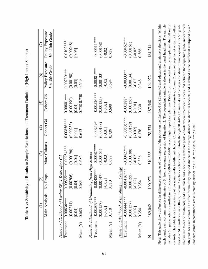
Tabl

eA

.9:S

ensi

tivity

ofR

esul

tsto

Sam

ple

Res

trict

ions

and

Trea

tmen

tDefi

nitio

n(H

igh

Impa

ctSa

mpl

e)

(1)

(2)

(3)

(4)

(5)

(6)

(7)

Mai

nA

naly

sis

No

Dro

psM

ore

Coh

orts

Coh

ortG

4C

ohor

tG6

Polic

yEx

posu

rePo

licy

Expo

sure

5th

-8th

Gra

de5t

h-1

0th

Gra

de

Pane

lA:L

ikel

ihoo

dof

Losi

ngSE

,4Ye

ars

afte

rG

5Tr

eatm

ent

0.00

836*

**0.

0083

5***

0.00

954*

**0.

0085

6***

0.00

801*

**0.

0073

0***

0.01

02**

*(0

.002

14)

(0.0

0206

)(0

.001

96)

(0.0

0253

)(0

.001

90)

(0.0

0198

)(0

.002

48)

[0.0

4][0

.04]

[0.0

4][0

.04]

[0.0

4][0

.03]

[0.0

5]M

ean

(Y)

0.68

30.

683

0.68

60.

613

0.75

80.

730

0.64

9

Pane

lB:L

ikel

ihoo

dof

Gra

duat

ing

from

Hig

hSc

hool

Trea

tmen

t-0

.005

09**

*-0

.004

88**

*-0

.005

87**

*-0

.002

59*

-0.0

0526

***

-0.0

0381

***

-0.0

0511

***

(0.0

0157

)(0

.001

47)

(0.0

0151

)(0

.001

38)

(0.0

0135

)(0

.001

33)

(0.0

0158

)[-

0.02

][-

0.02

][-

0.03

][-

0.01

][-

0.02

][-

0.02

][-

0.02

]M

ean

(Y)

0.71

00.

710

0.69

80.

739

0.69

00.

694

0.73

8

Pane

lC:L

ikel

ihoo

dof

Enro

lling

inC

olle

geTr

eatm

ent

-0.0

0444

***

-0.0

0416

***

-0.0

0427

**-0

.005

05**

*-0

.002

88*

-0.0

0333

**-0

.004

62**

*(0

.001

57)

(0.0

0155

)(0

.001

88)

(0.0

0159

)(0

.001

56)

(0.0

0134

)(0

.001

61)

[-0.

02]

[-0.

02]

[-0.

02]

[-0.

02]

[-0.

01]

[-0.

02]

[-0.

02]

Mea

n(Y

)0.

354

0.35

40.

336

0.37

60.

330

0.34

80.

366

N18

9,04

219

0,97

331

0,66

317

8,37

418

7,54

819

4,97

218

4,21

4

Not

e:Th

ista

ble

show

sdi

ffer

ence

-in-d

iffer

ence

ses

timat

esof

the

impa

ctof

the

polic

yon

the

likel

ihoo

dof

SEre

mov

alan

ded

ucat

iona

latta

inm

entd

ecis

ions

.With

inea

chpa

nel,

each

colu

mn

repo

rtses

timat

esof

d 1fr

oma

sepa

rate

regr

essi

onof

Equa

tion

2.Th

ede

pend

entv

aria

ble

issh

own

inth

epa

nelh

eadi

ngs.

The

sam

ple

incl

udes

5th

grad

eco

horts

enro

lled

inSE

betw

een

1999

-00

to20

04-0

5in

ourh

igh

impa

ctsa

mpl

e.Se

eTa

ble

2fo

rmor

ede

tail

onth

esa

mpl

ean

dth

efu

llse

tof

cont

rols

.Thi

stab

lete

stst

hese

nsiti

vity

ofou

rmai

nre

sults

todi

ffere

ntch

oice

s.C

olum

n1

isou

rbas

elin

ees

timat

es,C

olum

n2

does

notd

rop

the

seto

fdis

trict

outli

ers

base

don

SEen

rollm

enti

n20

04-0

5,C

olum

n3

incl

udes

coho

rtsfr

om19

96-0

7th

roug

h20

04-0

5,C

olum

ns4

and

5ch

ange

sth

esh

are

oftim

eex

pose

daf

ter5

thgr

ade

that

we

use

tode

fine

treat

men

ts,a

ndC

olum

ns6

and

7fo

cus

ondi

ffer

entg

rade

coho

rtsw

here

treat

men

tis

mea

sure

dbe

twee

nth

ere

spec

tive

grad

ean

dex

pect

ed9t

hgr

ade

fore

ach

coho

rt.Th

eef

fect

fort

hefu

llyex

pose

dst

uden

tatt

heav

erag

edi

stric

tare

show

nin

brac

kets

,and

isde

fined

asth

eco

effic

ient

mul

tiplie

dby

4.5.

Stan

dard

erro

rsin

pare

nthe

ses

are

clus

tere

dby

dist

rict.

*p<

0.10

,**

p<0.

05,*

**p<

0.01

.

61

Table A.10: Likelihood of Being Enrolled in SE in Fifth Grade

(1) (2)FRL 0.0187*** -0.00513***

(0.00119) (0.000919)

Immigrant -0.0301*** -0.0124***(0.00633) (0.00384)

Male 0.0370*** 0.0369***(0.000907) (0.000930)

ELL 0.0306*** -0.0332***(0.00620) (0.00345)

Native Amercian 0.00100 -0.00774(0.00532) (0.00530)

Asian -0.0491*** -0.0473***(0.00266) (0.00269)

Black 0.00651*** -0.0395***(0.00226) (0.00228)

Hispanic -0.0218*** -0.0421***(0.00168) (0.00156)

Std Red (G3) -0.0551***(0.00191)

Std Math (G3) -0.0279***(0.00121)

Constant -0.902*** -0.420***(0.0276) (0.0185)

N 1,345,875 1,345,875R-squared 0.038 0.106

Mean 0.0674 0.0674

Note: This table contains results from linear prediction models that predict SE participation in 5th grade based onbaseline demographics and achievement measured in 3rd grade. Standard errors in parentheses are clustered at thedistrict level. *p<0.10, ** p<0.05, *** p<0.01.

62

Tabl

eA

.11:

The

Impa

ctof

the

Polic

yon

SEPl

acem

enta

ndEd

ucat

iona

lAtta

inm

ent–

Acc

ount

ing

forD

iffer

ence

sin

Perf

orm

ance

inSE

Mon

itorin

g(H

igh

Impa

ctSa

mpl

e)

(1)

(2)

(3)

(4)

(5)

(6)

(7)

(8)

Pane

lA:L

ikel

ihoo

dof

Losi

ngSE

(by

Expe

cted

9th

grad

e)Tr

eatm

ent

0.00

836*

**0.

0070

5**

0.00

643*

*0.

0077

6***

0.00

794*

**0.

0090

0***

0.00

844*

**0.

0090

8***

(0.0

0214

)(0

.003

04)

(0.0

0284

)(0

.002

56)

(0.0

0227

)(0

.002

22)

(0.0

0231

)(0

.002

20)

[0.0

38]

[0.0

32]

[0.0

29]

[0.0

35]

[0.0

36]

[0.0

41]

[0.0

40]

[0.0

40]

Mea

n(Y

)0.

683

0.32

60.

338

0.68

30.

683

0.68

30.

683

0.68

3

Pane

lB:L

ikel

ihoo

dof

Gra

duat

ing

from

Hig

hSc

hool

Trea

tmen

t-0

.005

09**

*-0

.004

99**

-0.0

0419

**-0

.005

28**

*-0

.004

97**

*-0

.005

45**

*-0

.005

11**

*-0

.005

38**

*(0

.001

57)

(0.0

0211

)(0

.001

82)

(0.0

0186

)(0

.001

60)

(0.0

0164

)(0

.001

61)

(0.0

0163

)[-

0.02

2][-

.022

][-

.019

][-

0.02

4][-

0.02

2][-

0.02

5][-

0.02

3][-

0.02

4]M

ean

(Y)

0.71

00.

726

0.72

00.

710

0.71

00.

710

0.71

00.

710

Pane

lC:L

ikel

ihoo

dof

Enro

lling

inC

olle

geTr

eatm

ent

-0.0

0444

***

-0.0

0531

**-0

.006

23**

*-0

.006

22**

*-0

.003

98**

-0.0

0415

**-0

.004

35**

-0.0

0394

**(0

.001

57)

(0.0

0242

)(0

.002

15)

(0.0

0196

)(0

.001

72)

(0.0

0167

)(0

.001

70)

(0.0

0168

)[-

0.02

0][-

.024

][-

.028

][-

0.02

7][-

0.01

8][-

0.01

9][-

0.02

0][-

0.02

0]0.

354

0.37

10.

372

0.35

40.

354

0.35

40.

354

0.35

4

N18

9,04

211

5,24

214

4,04

018

9,04

218

9,04

218

9,04

218

9,04

218

9,04

2D

istr

ictS

ampl

eA

llX

XX

XX

XR

educ

eSe

para

teIn

stLo

wM

odifi

edTe

st-T

akin

gLo

wC

ontro

lsFu

llSe

tX

XX

XX

XX

Xf(

t)⇥

Mod

ified

Test

-Tak

ing

Xf(

t)⇥

Sepa

rate

Inst

ruct

ion

Xf(

t)⇥

Bla

ckO

verr

epre

sent

atio

nX

f(t)⇥

His

pani

cO

verr

epre

sent

atio

nX

Bla

ckO

verr

epre

sent

atio

n⇥

Frac

Expo

sed c

XH

ispa

nic

Ove

rrep

rese

ntat

ion⇥

Frac

Expo

sed c

X

Not

e:Th

ista

ble

show

sdi

ffer

ence

-in-d

iffer

ence

ses

timat

esof

the

impa

ctof

the

polic

yon

the

likel

ihoo

dof

SEre

mov

alan

ded

ucat

iona

latta

inm

entd

ecis

ions

.With

inea

chpa

nel,

each

colu

mn

repo

rtses

timat

esof

d 1fr

oma

sepa

rate

regr

essi

onof

Equa

tion

2.Th

ede

pend

entv

aria

ble

issh

own

inth

epa

nelh

eadi

ngs.

The

sam

ple

incl

udes

5th

grad

eco

horts

enro

lled

inSE

betw

een

1999

-00

to20

04-0

5in

ourh

igh

impa

ctsa

mpl

e.Se

eTa

ble

2fo

rmor

ede

tail

onth

esa

mpl

ean

dth

efu

llse

tof

cont

rols

.The

effe

ctfo

rthe

fully

expo

sed

stud

enta

tthe

aver

age

dist

ricta

resh

own

inbr

acke

ts,a

ndis

defin

edas

the

coef

ficie

ntm

ultip

lied

by4.

5.St

anda

rder

rors

inpa

rent

hese

sar

ecl

uste

red

bydi

stric

t.*p<

0.10

,**

p<0.

05,*

**p<

0.01

.

63

Table A.12: OLS and IV Estimates of the Impact of the Enrollment Target on Educational Attain-ment (Regular Math Test-Takers)

Y Mean SE Mean Y OLS FS RF IVGraduated HS 0.516 0.749 0.05347*** 0.01199*** -0.00758*** 0.6323**

(0.00542) (0.00325) (0.00196) (0.208)

College Enrolled 0.477 -0.06852*** -0.00479* 0.39962(0.00480) (0.00236) (0.238)

Kleibergen-PaapF-Statisitic 13.78

Notes: This table reports difference-in-differences estimates of the impact of the policy on SE removal (by expected9th grade) and educational attainment (Columns 1 -2). This table also reports OLS and IV estimates of SE removalon educational attainment outcomes (Columns 3-4). The dependent variable is shown in the row labels. The sampleincludes 5th grade cohorts enrolled in SE between 1999-00 to 2004-05 in our high impact sample who were taking theregular math test at baseline (i.e. 4th grade) (N=76,237). See Table 2 for more detail on the sample and for the full listof controls used. Standard errors in parentheses are clustered by district. *p< 0.10, **p < 0.05, *** p< 0.01.

Table A.13: Triple-Difference Estimates for SE Placement and Educational Attainment, RegularTest-Takers in 4th Grade only

SE Removal HS Grad College EnrolledTreatment 0.0143*** -0.00736*** -0.00476*

(0.00320) (0.00212) (0.00261)

Treatment ⇥ Std Test Score (G4) 0.00410*** -0.000440 0.00148(0.00103) (0.000816) (0.00101)

Mean 0.484 0.749 0.479

N 65,937 65,937 65,937

Notes: This table contains results obtained from a triple difference model where we augment Equation 2 by includinga term that interacts 4th grade standardized math test scores from fourth grade with treatment and lagged 4th gradestandardized math test scores from fourth grade. See Table 2 for the full list of controls and information about each ofthese outcome variables. The sample for these regressions includes students who were taking the unmodified mathexam during 4th grade in SE cohorts between 2000 and 2005. Standard errors in parentheses are clustered at the districtlevel. *p< 0.10, **p < 0.05, *** p< 0.01.

64

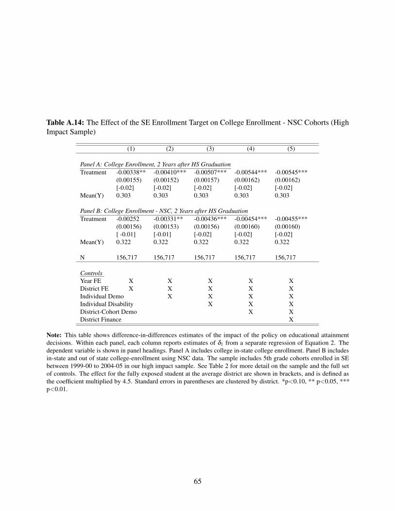
Table A.14: The Effect of the SE Enrollment Target on College Enrollment - NSC Cohorts (HighImpact Sample)

(1) (2) (3) (4) (5)

Panel A: College Enrollment, 2 Years after HS GraduationTreatment -0.00338** -0.00410*** -0.00507*** -0.00544*** -0.00545***

(0.00155) (0.00152) (0.00157) (0.00162) (0.00162)[-0.02] [-0.02] [-0.02] [-0.02] [-0.02]

Mean(Y) 0.303 0.303 0.303 0.303 0.303

Panel B: College Enrollment - NSC, 2 Years after HS GraduationTreatment -0.00252 -0.00331** -0.00436*** -0.00454*** -0.00455***

(0.00156) (0.00153) (0.00156) (0.00160) (0.00160)[ -0.01] [-0.01] [-0.02] [-0.02] [-0.02]

Mean(Y) 0.322 0.322 0.322 0.322 0.322

N 156,717 156,717 156,717 156,717 156,717

ControlsYear FE X X X X XDistrict FE X X X X XIndividual Demo X X X XIndividual Disability X X XDistrict-Cohort Demo X XDistrict Finance X

Note: This table shows difference-in-differences estimates of the impact of the policy on educational attainmentdecisions. Within each panel, each column reports estimates of d1 from a separate regression of Equation 2. Thedependent variable is shown in panel headings. Panel A includes college in-state college enrollment. Panel B includesin-state and out of state college-enrollment using NSC data. The sample includes 5th grade cohorts enrolled in SEbetween 1999-00 to 2004-05 in our high impact sample. See Table 2 for more detail on the sample and the full setof controls. The effect for the fully exposed student at the average district are shown in brackets, and is defined asthe coefficient multiplied by 4.5. Standard errors in parentheses are clustered by district. *p<0.10, ** p<0.05, ***p<0.01.

65