the low-energy electronic structure of s^r^oyqmlab.ubc.ca › arpes › publications › mstheses...

The Low-Energy Electronic Structure of S^R^Oy: An ARPES and XAS Study

by

M. A. Hossain

B.Sc, The University of Dhaka, 2001 CASM, The University of Cambridge, 2002

A THESIS SUBMITTED IN PARTIAL FULFILMENT OF THE REQUIREMENTS FOR THE DEGREE OF

MASTER OF SCIENCE

in

The Faculty of Graduate Studies

(Physics)

THE UNIVERSITY OF BRITISH COLUMBIA

April 20, 2005

© M. A. Hossain, 2005

11

Abstract S r 3 R u 2 0 7 has recently attracted a lot of research effort primarily due to the discovery of magnetic field tuned quantum criticality at low temperature [7, 8]. To understand the mechanism driving the system to this critical point, we need precise information on the low energy electronic excitations, electronic correlation effects and local electronic structure of the system, which are still a subject of intense debate. To address these issues we employed three powerful theoretical and experimental techniques: Density Functional Theory (DFT), Angle Resolves Photoemission Spectroscopy (ARPES) and X-Ray Absorption Spectroscopy (XAS). The band structure calculations were done using the T B - L M T O - A S A (tight binding-linear muffin tin orbital-atomic sphere approximation) approach [34]. Our result agreed very well with the previous calculations [30, 31, 41, 42]. The Density of States (DOS) data were used to interpret the angle dependence of X A S data. We begin with an analysis of the metallic ground state and hybridization between the orbitals in S r 2 R u 0 4

using the X A S data. The same line of analysis was used to interpret S r 3 R u 2 0 7 X A S data. Our data clearly shows the extra features expected due to the presence of a new oxygen site in S r 3 R u 2 0 7 with respect to S r 2 R u 0 4 . With A R P E S we obtained the first high resolution Fermi surface of S r 3 R u 2 0 7 and quasiparticle band dispersion. The overall low energy electronic structure appears to be in agreement with the band structure calculations of Singh et. al. [30].

iii

Contents

Abstract ii

Contents iii

List of Figures iv

Acknowledgements vii

1 Introduction 1

2 Angle Resolved Photoemission Spectroscopy (ARPES) 3 2.1 Kinematics of photoemission 3 2.2 Theory: spectral representation 5 2.3 Photoemission intensity 8 2.4 Lineshape analysis 11

3 X-ray Absorption Spectroscopy (XAS) 14 3.1 X-ray absorption process 15 3.2 XAS matrix element 16 3.3 Angular dependence of XAS spectra 17

4 Strontium Ruthenate: Physical Properties 19 4.1 Crystal structure 20 4.2 Resistivity 22 4.3 Magnetic susceptibility and specific heat 24 4.4 Our sample 25

5 Strontium Ruthenate: Electronic Structure 26 5.1 Quantum chemistry and magnetism 27 5.2 Calculations and experiments 28 5.3 XAS on strontium ruthenate 29 5.4 ARPES on strontium ruthenate: the Fermi surface 39 5.5 Outlook: ARPES Lineshape Analysis of Strontium Ruthenate . . . . 42

Bibliography 43

iv

List of Figures

2.1 Energetics of the photoemission process from Ref. [14]. The electron energy distribution produced by the incoming photons, and measured as a function of the kinetic energy Eki„ of the photoelectrons (right), is more conveniently expressed in terms of the binding energy EB (left) when one refers to the density of states in the solid (EB = 0 at Ep). Ep, EQ and Ev correspond to the Fermi energy, bottom of the valence band and the vacuum level respectively 4

2.2 (a) geometry of an A R P E S experiment, (b)momentum-resolved one electron removal and addition spectra for a noninteracting electron system with a single energy band dispersing across Ep,{c) same spectra for an interacting Fermi-liquid system, (d) photoemission spectrum for gaseous system. Figure taken from Ref. [13] 9

3.1 Schematic description of the x-ray absorption process: an electron is excited from the core level to the unoccupied states in the conduction band by absorbing a photon with energy hu, leaving a hole in the core level. Such an electron-hole pair may decay through either x-ray fluorescence or emission of Auger electrons. Adapted from Ref. [22]. . 14

4.1 S r 2 R u 0 4 crystal structure showing two non-equivalent oxygen sites [32]. 19 4.2 S r 3 R u 2 0 7 crystal structure showing three non-equivalent oxygen sites

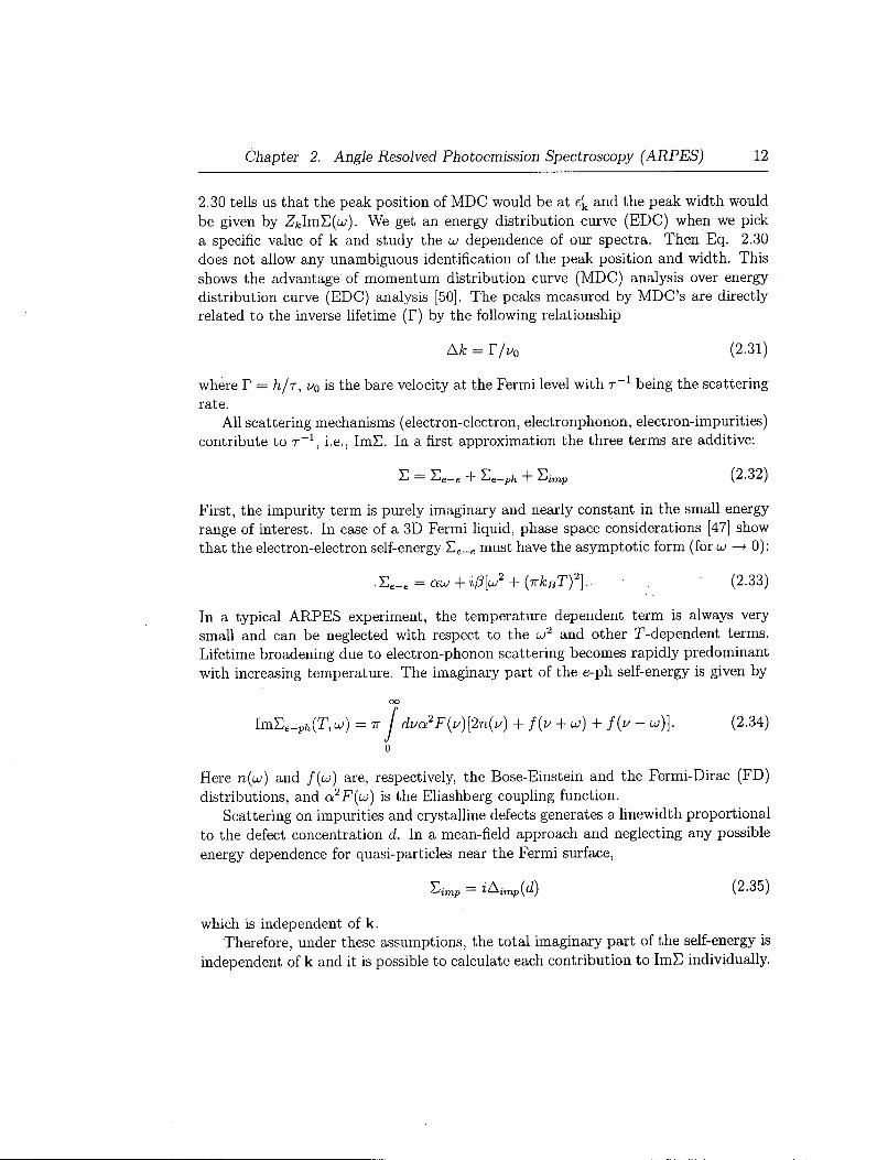
[41] 4.3 The supercell used in the present work following. The corresponding

lattice parameters are \f2a0 x \/2oo x co> rendering a volume which is twice the volume of the undistorted IA/mmm unit cell (Fig. 4.2). The large ratio of the ionic radii of Ru (center of octahedron) to Sr (spheres) places the Ru-0(3) planes under compression. To relieve some of this pressure, the crystal structure responds by rotations (arrows) of the octahedra around the c axis. Taken from Ref. [24] 21

4.4 The electrical resistivity of FZ crystals of S r 3 R u 2 0 7 above 0.3 K . Both pab and pc are shown. The inset shows the low-temperature electrical resistivity against the square of temperature T 2 [25] 22

20

List of Figures v

4.5 The magnetic susceptibility of FZ crystals of Sr3Ru 2 0 7 . The inset shows the low temperature magnetic susceptibility against tmeperature T [25] 23

4.6 The specific heat divided by temperature, Cp/T of FZ crystals of S r 3 R u 2 0 7 [25] 24

4.7 Resistivity versus temperature for two S r 3 R u 2 0 7 crystals. The upper curve is a crystal grown under 100% 0 2 atmosphere and the lower curve is our sample grown under optimised conditions (10% 0 2 + 90% Ar). The dotted lines are Fermi liquid T2 fits to the data between 4K and8K[9] 25

5.1 In the octahedral crystal field, the fivefold degeneracy of d orbital is lifted to two ea orbitals (dx2_y2 and d3z2_T2) and three £ 2 f l orbitals (dxy,dyz and dzx). Taken from Ref. [28] 26

5.2 Panel (a): Density of states plot of Ru in S r 2 R u 0 4 . Panel (b): Density of states plot of Ru in S r 3 R u 2 0 7 30

5.3 O Is X A S of S r 2 R u 0 4 at ^ = 0°, 50°, 80° fitted by a set of gaussians. The angle 9i denotes the angle between the incident beam and the surface normal and all data were taken at 50 K , 0 Tesla 31

5.4 O Is N E X A F S of S r 2 R u 0 4 . The spectra labelled T E Y are taken using the total electron yield method, while the spectra labelled F Y were taken using the fluorescence yield mode [29] 32

5.5 Panel (a): Density of states of in-plane oxygens (0(1)) in S r 2 R u 0 4 . Panel (b): Density of states of apical oxygens (0(2)) in S r 2 R u 0 4 . . . 33

5.6 Sum of the densities of states of oxygen. pXiV sum denotes the sum of px and py DOS of the in-plane (0(1)) and apical oxygens (0(2)) multiplied by a step function that is zero below EF. pz sum denotes the sum of pz DOS of 0(1), 0(2) also multiplied by a step function that is zero below Ep. The inset zooms into the region of our interest. It is important to note that according to the core level shifts, 0(1) has been shifted by 1.33 eV 34

5.7 Panel (a): Density of states plot of between-plane oxygens (0(1)) in S r 3 R u 2 0 7 . Panel (b): Density of states plot of apical oxygens (0(2)) in S r 3 R u 2 0 7 . Panel (c): Density of states plot of in-plane oxygens (0(3)) in S r 3 R u 2 0 7 35

List of Figures vi

5.8 Sum of the densities of states of oxygen. pXiV sum denotes the sum of px and py DOS of 0(1), 0(2) and 0(3) multiplied by a step function that is zero below Ep• pz sum denotes the sum of pz DOS of 0(1), 0(2) and 0(3) also multiplied by a step function that is zero below Ep. The inset zooms into the region of our interest. It is important to note that according to the core level shifts, O(l) and 0(3) has been shifted by 0.68 eV and 1.17 eV respectively. Therefore, steps are visible at 0 eV (due to Fermi function), 0.68 eV (due to core level shift in 0(1)) and 1.17 eV (due to core level shift in 0(3)) 36

5.9 O Is N E X A F S of S r 3 R u 2 0 7 at 0* = 0°, 20°, 35°, 82° fitted by a set of gaussians. A l l data were taken at 50 K , 0 Tesla 37

5.10 Panel (a): in the quadrant of the 2D BZ, the a,/3, and 7 sheets of FS are indicated. Panel (b): Ep intensity map. Primary a, (3, and 7 sheets of FS are marked by red lines, and replica due to surface reconstruction is marked by yellow lines. A l l data were taken on Sr2Ru0 4 cleaved at 10 K . Panel (c): EF intensity map. A l l data were taken at 10 K on S r 2 R u 0 4 cleaved at 180 K [33]. 39

5.11 Panel (a): Fermi surface of S r 3 R u 2 0 7 in the ideal tetragonal structure. Panel (b): Fermi surface of S r 3 R u 2 0 7 in the ideal tetragonal structure folded into the orthorhombic zone. Panel (c): Fermi surfaces of S r 3 R u 2 0 7 in the experimental orthorhombic structure. Note that in Panel (b) and (c) the zone is rotated 45° with respect to the tetragonal and folded. Panel (d) Same as in Panel (c) but with filled areas indicating the effect of 5 meV upwards and downwards shifts of Ep [30]. 40

5.12 A comparison of the measured Fermi surface to the one calculated by Singh et. al. [30] 41

vu

Acknowledgements

First, I would like to thank my supervisor Prof. Andrea Damascelli for countless stimulating discussions, for his sharp and insightful criticism and most importantly, for his great effort to train me as an experimentalist. I am greatly indebted to Ilya Elfimov for his help with the T B - L M T O - A S A program and elucidating the meaning of the DOS plots.

I thank Prof. George Sawatzky for his wonderful Solid State Physics Courses and Prof Johannes Barth for helpful suggestions regarding the thesis. Special thanks to all the members of Damascelli-Sawazky group Jeff Mottershed, Mauro Plate, David Hawthorn, Nicholas Ingle and Andreas Riemann.

The warm hospitality of the B A C H beamline scientists, Federica Bondino, Marco Zangrando, Michele Zacchigna and Fulvio Parmigiani made my first beamtime experience an enjoyable one. I am fortunate to be able to work with Donghui L u at SSRL and Nicholas Ingle, Felix Baumberger and Worawat Meevasana at Prof. Z.-X. Shen's lab, Department of Physics, Stanford University. Finally, I would like to thank Arefa and Ryan for their continuing support and inspiration.

Chapter 1

i

Introduction

Complex oxide systems such as the cuprates, nickelates, and manganites have generated intense study over the last decade. The efforts were, first, to clarify the relationship between the exotic phases of the materials and second, to elucidate the origin and nature of the rich phenomena these compounds exhibit [1], such as unconventional superconductivity, charge and orbital ordering, and colossal magnetoresistance.

More recently, the attention to 4c! transition-metal oxides (TMO) has increased because of numerous intriguing properties, such as superconductivity [4] non-Fermi liquid behavior [10] and metal-insulator transitions have been observed in ruthen-ates and molybdates. The 4d T M O are characterized by more extended orbitals than those of 3d T M O . So, it is generally believed that electrons in the extended 4d orbitals feel weak on-site Coulomb repulsion energy and that the 4d orbitals hybridize more strongly with neighboring orbitals, e.g., oxygen 2p orbitals, than 3d orbitals. However, these qualitative ideas are not sufficient to understand the intriguing physical phenomena observed in some Ad T M O . Quantitative information on physical parameters related to the electronic structures of T M O will serve as a starting viewpoint in investigating various 4d T M O with a potential to discover other new interesting phenomena. They will also allow us to make comparisons with the 3d T M O cases, which can provide us with a better understanding on the strongly correlated electron systems.

Among these 4d T M O Strontium-ruthenium oxides of the Ruddlesden-Popper type compound series of S r n + i R u „ 0 3 n + i with perovskite based crystal structure have been a focus of intensive research due to their diverse and surprising properties. For example, S rRu0 3 is a rare example of an itinerant ferromagnet based on 4d electrons [2, 3]. S r 2 R u 0 4 is isostructural to the high-Tc compound L a 2 _ x B a x C u 0 4 and has the layered perovskite structure with a single R u 0 2 plane per formula unit. It is strongly two dimensional, and shows a Pauli like paramagnetic susceptibility [4]. It is best known for its unconventional superconductivity [4], which is thought to involve spin triplet pairing [5]. Structural distortions in Sr-based ruthenates.are either small or absent. Substituting Ca for Sr, however, introduces larger rotations of the Ru-O octahedra since Ca has a much smaller atomic radii than Sr. This causes the bandwidth to narrow and changes to the crystal field splitting. Thus, although Ca and Sr are both divalent cations, the properties of the Ca-based materials are markedly different than Ru-based materials. C a R u 0 3 is a paramagnetic metal with a large mass enhancement [6], while C a 2 R u 0 4 is an antiferromagnetic insulator [36]. This diversity

Chapter 1. Introduction 2

shows that the ruthenates are characterized by a series of competing instabilities, giving a clear motivation for the careful investigation of all the compounds in the series. An even more important feature of the ruthenates is that, in contrast to 3d oxides such as the manganites and many cuprates, no explicit chemical doping is required to produce metallic conduction. One other advantage is that these materials can be grown in extremely pure form with very low disorder and impurities [9]. This gives a unique opportunity to probe a wide range of correlated electron physics in the low disorder limit.

In this thesis we are investigating one of the most intriguing members of this family: S r 3 R u 2 0 7 . This system has been a subject of intense research when it became clear that this material exhibits behavior consistent with proximity to a metamagnetic (i.e., magnetic field tuned) quantum critical point [7, 8]. In the following chapters we shall introduce the experimental and theoretical techniques that we used to investigate the properties of S r 3 R u 2 0 7 , namely, angle resolved photoemission spectroscopy (ARPES) and X-ray absorption spectroscopy (XAS). This shall be followed by an introduction to the physical properties of Sr 3 Ru 2 07. After that we shall discuss the results of our experiments and band theory calculations.

3

Chap te r 2

A n g l e Resolved Pho toemiss ion Spectroscopy ( A R P E S )

The great success of Angle Resolved Photo-Emission Spectroscopy (ARPES) in the study of solids can be attributed to the capacity of this technique to yield direct access to the energy and momentum of the occupied electronic states. This chapter should serve as an introduction to A R P E S and we want to answer the following basic question: What are we actually measuring in angle resolved photoemission?

We will see that A R P E S measurements have a simple interpretation within the framework of one-electron band theory, i.e., it maps the band structure of the material and, therefore, the Fermi surface. This aspect of A R P E S data analysis has been extensively used in Chapter 5. But, in future, we are more interested to use this technique to study the complex many-body physics of S r 3 R u 2 0 7 . Keeping that goal in mind, we introduce the idea of single-particle spectral function and show that the intensity in a photoemission experiment corresponds to the electron removal part of the spectral function modulated by transition matrix elements. Since spectral function is directly related to self energy which in turn contains all the interactions present in a system, the analysis of A R P E S spectra can provide us with direct information about the dominant interactions present in a system as a function of temperature. We conclude this chapter by a discussion on the subtle issues of A R P E S lineshape analysis to extract information about the self energy of our system. This discussion is based on recent works by N . J. C. Ingle et. al. [50].

2.1 Kinematics of photoemission

When light is incident on a sample, an electron can absorb a photon and escape from the material with a maximum kinetic energy of hu — 4> where u is the frequency of the incident photon and <p is the work function of the metal. The energetics of this photoemission process is sketched in Fig. 2.1.

In an A R P E S experiment, a beam of monochromatic radiation is incident on a sample and, as a result, electrons are emitted by the photoelectric effect and escape into the vacuum in all directions. By collecting photoelectrons with an electron energy analyzer we measure the kinetic energy Ekm of the photoelectrons for a given emission angle. This way the photoelectron momentum in vacuum p is also completely

Chapter 2. Angle Resolved Photoemission Spectroscopy (ARPES) 4

KB

N(E)

Figure 2.1: Energetics of the photoemission process from Ref. [14]. The electron energy distribution produced by the incoming photons, and measured as a function of the kinetic energy Ekin of the photoelectrons (right), is more conveniently expressed in terms of the binding energy EB (left) when one refers to the density of states in the solid (EB = 0 at Ep). Ep, Eo and Ev correspond to the Fermi energy, bot tom of the valence band and the vacuum level respectively.

determined |p| = p = V^mEkin (2.1)

and and p± are determined from the polar (6) and azimuthal (4>) emission angles. Our target now is to construct the electronic dispersion relation of the solid we are

probing from this information. To be more specific, we need to find out the relation between binding energy EB and momentum k for the electrons propagating inside the solid, starting from Ekin a n d p measured for the photoelectrons in vacuum. The photon momentum can be neglected at low photon energies typical ly used in A R P E S experiments. Therefore, exploiting the energy and momentum conservation laws, we


can get the following relations

Ekin = hv-<j>- \EB\ (2.2).

PH = Uk\\ = y/2mEkin- s'm9 (2.3)

where py is the component parallel to the surface of the electron crystal momentum in the extended-zone scheme. Detailed description of the photoemission process and assumptions behind deriving these relationships can be found in Ref. [12].

To examine the standard interpretation of angle resolved photoemission (ARPES) data from a theoretical point of view let us start with the idea of single-particle spectral function.

2.2 Theory: spectral representation One of the most powerful tools available to a many-body physicist is the single-particle spectral function [15]. To illustrate what this is we can start with the spectral decomposition of a time dependent function, f(t), into the sum of its components at various frequencies:

oo

/(£) = J F{uj)eiwtduj (2.4) —oo

where F(to) gives the spectrum of /(£). Let us try to evaluate a similar form of decomposition for the propagator or

Green's function Q(k,uj) at zero temperature. A Green's function can tell us how an initial probability amplitude function evolves in time and space. We start out with a particle wave in space-time. This is propagated forward (in most cases) in time to a final wave using Greens function. The final wave is then used to calculate expectation values of observables. In particular, we are interested in calculating the probability for a wave to scatter off of a target into a particular state. Let {ip^} an<^ E% be the exact eigenstate and energies of the Hamiltonian H of the interacting ./V particle system. The single particle propagator or Green's function can be defined as

G{k2,k1,t2 - *i) = C7+(k 2 ,k 1 , i 2 - h)t2>tl

+G-(k2,k1,t2-t1)t2<tl. (2.5)

where G~(k2,ki, t2 — ti) is the probability amplitude that if at time t\ we remove a particle in (p^ (add a hole in </>kl) from the interacting system in its ground state, then at time t2 the system will be in its ground state with an added hole in </>k2. Thus, G _ ( k 2 , k 1 , i 2 — ti) is just the hole propagator. Similarly, G + ( k 2 , k i , i 2 — ^i) is the


electron propagator. Here <£k. are the eigenstates of the unperturbed single particle Hamiltonian.

Q(k2, k i , £2 — ^1) can be expressed in terms of creation and annihilation operators c k i and cl.:

G(k2,k1,t2-h) = -iQ{t2 - h^M^Mcl^h)^)

+iQ(h - i2)(V'ol41(ii)ck 2(i2)|V'o). (2.6)

where \ip0) is the ground state wave function of the system and Q is the step function. Let tx = 0 and t2 = t. Then

G~(k,t) =iG(-t)

x E ^ l ^ l ^ - 1 ) ^ " 1 ! ^ - ^ ! ^ ) n

= iB{-t) £ -l\cM)\2e-^~B"^ n

= iO(-t)J2\(cKU\2e-«E°N-E"-^ (2.7) n

Taking Fourier transform of Eq. (2.7) we find

°- ( fc .»)-Eiw- i ' M - ( f f -V-) -« ( 2 ' 8 )

where EQ and E Q - 1 are the ground state energies of interacting ./V and N — 1 particle systems respectively.

For large N, these results can be expressed in terms of chemical potential /i, EQ — E % - 1 = E» - Eg'1 + Et1 - E^"1 = u.N~l - u»0-1 = n- unQ. This gives

G-(k,t) = i G ( - i ) E l ( c k ) n 0 | 2 e - ^ — > « (2.9) n

and G - ( k l W ) = J ] | (c k )„„ | 2 1 . (2.10)

^ LU - (fl- LOn0) - 10

The spectral function is defined as:

A- (k ,o , )= ^ | ( c k ) n 0 | 2 (2.11)


or, equivalently, A~(k,Lo) = \(cuU\26(u - LunQ). (2.12)

n

where u> > 0. It gives the probability that the state \IJJQ) with an added hole in state k is an exact eigenstate of the (N — l)-particle system with energy between u> and LO + did.

In a system with large volume, the energy levels are so closely spaced that we can go from a sum to an integral. Therefore, substituting Eq. (2.11) in Eq. (2.9) and (2.10), we can express G~ in terms of spectral function:

oo

G " ( M ) = iQ{-t) J A-^toy-^-^duj (2.13) o

oo _ (

G - ( k , W ) = / <ti f ^ u ) (2.14) J LO — (/i — LO j — 10 0

The retarded Green function is defined as

G{k,Lo) = G+{k,Lo) + [G-(k,w)]*.

Hence, in terms of the spectral function

G(k,L0) = j " A+(k,Lo') + A-(k,u)

dw o

LO — LO' — jl + i5 LO + LO1 — /x — iSj (2.15)

A comparison of Eq. 2.13 with 2.4 suggests that indeed A(k, to) is giving the spectrum of G(k, t). We can now make use of the following identity

1 =pl-\±m5(x) x±i5 \x j

where V denotes the Cauchy principal value [16], to get

A+(k,LJ-lj.) = --ImG(k,u>), u>n (2.16)

A-(k,fi-u) = +-lmG[k,u), to < /* (2.17) 7T


Hence we can define the full spectral function A(k, ui) as:

A(k,u>) = A+(k,to)+A-{k,Lo) = - - ImG(k ,u ; ) . (2.18) TT

The effect of electron-electron correlation to the Green function can be expressed in terms of the electron proper self energy

£(k,w) =ReE(k,w) +iImE(k,w).

Its real and imaginary parts contain all the information on the energy renormaliza-tion and lifetime, respectively, of an electron with band energy e k and momentum k propagating in a many-body system. The Green function can be expressed in terms of self-energy as

G(k,u;) = 1 . (2.19) u> — e k — h(K,ui)

Since A(k,ui) = - £ i m G ( k , w ) ,

A ( v s 1 . Im£(k,a>) . 1 ' ° J > . Tr [to - ek - ReS(k, u>)f + [ImE(k, to)f' ' K ' '

In (2.9), if there is no interaction, then ( c k ) n 0 = 5kn, i.e., ( c k ) n 0 is finite and equal to 1 only for a single energy level. But with interaction, in typical cases ( c k ) n 0 is spread out over a band of energy levels from say n to n", having width AE — u>n»i0 — uin><0.

2.3 Photoemission intensity To describe the photoemission process, we can start with how to calculate the transition probability wno at T = 0 for the optical excitation between the iV-electron ground state and one of the possible final state | ^ ) . This can be approximated by Fermi's golden rule

9-7T

^ n o = T\(^\Hint\^)\25(E» - < - hu) (2.21) where EQ = EQ~1 — EB and E% = E ^ ~ L + E K I N are the initial and final-state energies of the TV-particle system (EB is the binding energy of the photoelectron with kinetic energy ^fc i nand momentum k). The interaction of the the electromagnetic wave,i.e. photon, can be treated as a perturbation given by

- = 2 ^ ( A - P + P - A ) = ^ A ' P (2.22)


Photoemission geometry Non-interacting electron system Fermi liquid system

Figure 2.2: (a) geometry of an A R P E S experiment, (b)momentum-resolved one electron removal and addition spectra for a noninteracting electron system with a single energy band dispersing across Ep,(c) same spectra for an interacting Fermi-liquid system, (d) photoemission spectrum for gaseous system. Figure taken from Ref. [13].

where p is the electronic momentum operator and A is the electromagnetic vector potential.

The standard model of approximating the photoemission process is known as three-step model. Within this approach, the photoemission process is divided into three independent and sequential steps

• optical excitation of the electron to the bulk,

• travel of the excited electron to the surface and

• escape of the photoelectron into vacuum.

The total photoemission intensity is then given by the product of the probabilities of these three independent processes.

In evaluating the first step, and therefore, the photoemission intensity in terms of the transition probability wn0, it would be convenient to factorize the wavefunc-tions in Eq. (2.21) into photoelectron and (N — l)-electron terms. But doing this is not simple because the system will relax. The problems is simplified within the sudden approximation which applies to high kinetic energy electrons. In this limit, the photoemission process is assumed to be sudden, with no post-collisional interaction between the photoelectron and the system left behind. Then the final state can be written as

^ = M^-' (2-23)

where A is an antisymmetric operator that properly antisymmetrizes the iV-electron wavefunction so that Pauli principle is satisfied, is the wavefunction of the photoelectron with momentum k, and is the final state wavefunction of the (N — 1)-electron system left behind which can be chosen as an excited state with energy


E^~l, The total transition probability is then given by the sum over all possible excited states n.

Let us also write the initial state as the product of a one-electron orbital and an (N — l)-particle term 4>Q~1

^ = A ^ ' \ (2.24)

However, TPQ"1 can be expressed as

We should note that ipQ-1 may not be an exact eigenstate of the (N — l)-particle system left by the photoelectron. At this point we can write the matrix element of Eq. (2.21) as

( ^ \ H M \ ^ ) = < t o „ t | ^ > < V ^ W _ 1 > (2-25) where {^Hintl^o) = M%0 is the one-electron dipole matrix element, and the second term is the (N — l)-electron overlap integral. This whole analysis holds even if our initial state is an excited state of the system instead of being the ground state.

The total photoemission intensity measured as a function of Ekin a t a momentum k is

/(k, Ekin) = wn>i oc | M n

k / lj2 \cm,iMEkin + E^-1 - E% - hv) j (2.26) n, i n,i \ m /

where the sum is over an initial state i and | c m > i | 2 = \(il>m~1\ipif~1)\2 is the probability that the removal of an electron from state i will leave the (N — l)-particle system in the excited state m.

Comparing the term inside the parenthesis of Eq. (2.26) with Eq. (2.12), we see that an A R P E S spectrum actually measures the spectral function:

/ ( k , £ f c i n ) = 53|M^|M-(klW) (2.27) n,i

So far we have only discussed about direct photoemission (photon in, electron out). If we repeat the whole calculation starting from C?+(k, t) we can show that inverse photoemission (electron in, photon out) measures A+(k,tu). Also G(k,t,t) is a linear response function to an external perturbation. Therefore, the real and imaginary parts of its Fourier transform G(k, to) have to satisfy causality and hence related by Kramers-Kronig relations. This implies that if we have the full A(k,w) available from direct and inverse photoemission, we can calculate ReG(k, ui) and then obtain the full self energy directly from Eq. (2.19).

The finite temperature effects can be taken into account by implying the sudden


approximation again and the intensity measured in an A R P E S experiment can be written as

I(k,Ekm) = ]T \M^\2A(k,u;)f(u), (2.28) n,i

where f ( t o ) is the fermi function.

2.4 Lineshape analysis In real systems there are many factors that can contribute to the A R P E S spectra. First, the presence of interactions in the system broadens the spectra from a delta function shape to a finite width spectra (Fig. 2.3 (b), (c)). Therefore, the width of A R P E S lineshape reflects the nature of the interactions present in the system we are looking at. Also, the final state lifetime of the photoelectrons adds to the total A R P E S linewidth. The final state energy width is mixed in with a weight factor of Vh±/ve±, where Vh± and ve_i are the band velocities, perpendicular to the surface, of the photohole and photo electron, respectively. Therefore, the effect of the final electron state broadening can be suppressed if Vh± <C ve± [45]. This is why detailed photohole line-shape studies can only be done on surface states or layered systems like Ruddlesden-Popper type compound series of S r n + 1 R u n 0 3 n + 1 . Also, A R P E S spectrometer's finite resolution adds to the total A R P E S linewidth. Considering these effects, Eq. 2.28 can be written as [50]:

/(k, Ekin) = [J 0(k, iy)A{k, w)/(w) + B] ® R(Ak, Acu) (2.29)

where I0(k,u) = J2n t. j M ^ J 2 , B is the generic background and R(Ak,Au) is the experimental momentum and energy resolution, i.e., the response function of the instrument. Now in case of a Fermi liquid system, assuming that the self-energy (£) is a very slowly varying functions of k, Eq. 2.20 can be written in a form specially suitable for A R P E S analysis:

A(k,co) = Z/^K( M 2 + ^ H (2-30) 7r [ w - e ' kJ 2 + ]ZfcIm£(u>)]2

where Zk is the coherence (or renormalization) factor (1 — <9£'/du>)~1 and the renormalized band energy is ek = Zke^. This equation shows that we can expect Lorentzian shape for the A R P E S spectra where the peak width would correspond to the imaginary part of the self energy.

If we pick a specific value of ui and study the k dependence of the spectra, the resulting spectra is called the momentum distribution curve (MDC). In this case Eq.


2.30 tells us that the peak position of M D C would be at e'k and the peak width would be given by ZfcImS(u>). We get an energy distribution curve (EDC) when we pick a specific value of k and study the to dependence of our spectra. Then Eq. 2.30 does not allow any unambiguous identification of the peak position and width. This shows the advantage of momentum distribution curve (MDC) analysis over energy distribution curve (EDC) analysis [50]. The peaks measured by MDC's are directly related to the inverse lifetime (T) by the following relationship

Ak = r > 0 (2.31)

where T = h/r, v0 is the bare velocity at the Fermi level with r _ 1 being the scattering rate.

A l l scattering mechanisms (electron-electron, electronphonon, electron-impurities) contribute to r _ 1 , i.e., ImE. In a first approximation the three terms are additive:

£ = £ e - e ~t" £ e - p / i "f - Ejmp (2.32)

First, the impurity term is purely imaginary and nearly constant in the small energy range of interest. In case of a 3D Fermi liquid, phase space considerations [47] show that the electron-electron self-energy £ e _ e must have the asymptotic form (for u> —> 0):

. £e_e = auj + i(3[u2 + (nkBT)2}. • (2.33)

In a typical A R P E S experiment, the temperature dependent term is always very small and can be neglected with respect to the to2 and other T-dependent terms. Lifetime broadening due to electron-phonon scattering becomes rapidly predominant with increasing temperature. The imaginary part of the e-ph self-energy is given by

oo

ImEe_pfc(r,a;) = 7r jdva2F(u)[2n{v) + f[y + u>) + f(y - to)}. (2.34) o

Here n(u>) and f(u>) are, respectively, the Bose-Einstein and the Fermi-Dirac (FD) distributions, and a2F(u>) is the Eliashberg coupling function.

Scattering on impurities and crystalline defects generates a linewidth proportional to the defect concentration d. In a mean-field approach and neglecting any possible energy dependence for quasi-particles near the Fermi surface,

S i m p = iAimp(d) (2.35)

which is independent of k. Therefore, under these assumptions, the total imaginary part of the self-energy is

independent of k and it is possible to calculate each contribution to ImE individually.


This can be used to find out what type of interactions are most dominating in our system at a certain temperature.

14

Chapter 3

X-ray Absorption Spectroscopy (XAS)

The X-ray absorption process is a photon induced excitation of a core electron to an empty state above the Fermi level. In X-ray Absorption Spectroscopy (XAS) the absorption of x-rays due to this excitation process is measured as a function of photon energy, close to a core level binding energy. This probes the unoccupied states and is therefore complementary to photoemission. X A S has become a very powerful technique in the investigation of the unoccupied states above Ep after highly monochromatic, linearly polarized, easily tunable intense light from synchrotron ra-

a) Relaxation processes

E Y 8

VB

Participator

Auger

I".

core level -<»

Spectator

4 A _

hv

b) X-ray absorption and multiple electron scattering:

sample atoms

£ Electron Hole 4 ^ election mean free path

Figure 3.1: Schematic description of the x-ray absorption process: an electron is excited from the core level to the unoccupied states in the conduction band by absorbing a photon with energy hv, leaving a hole in the core level. Such an electron-hole pair may decay through either x-ray fluorescence or emission of Auger electrons. Adapted from Ref. [22].

Chapter 3. X-ray Absorption Spectroscopy (XAS) 15

diation sources became available. Near-edge x-ray absorption fine structure spectroscopy (NEXAFS) covers an energy range from the absorption threshold to the point at which the extended x-ray absorption fine structure (EXAFS) begins (normally a few tenths of eV above Ep).

3.1 X-ray absorption process

When the energy of an incident x-ray photon exceeds the binding energy of a particular core level, the photon can be absorbed, and the core electron is excited to an unoccupied state, leaving a hole in the core level. This process is illustrated in Fig. 3.1. Such a core hole may decay through x-ray fluorescence or Auger electron emission. The ionized atom may relax by occupation of the core hole with an electron from the valence band (VB), while the generated energy will normally not be used for the emission of a flourescence photon (probability 1%), but will be absorbed for the vaccum emission of an Auger electron (probability 99%) from the valence band. In case of a non-sufficient energy for the emission of the primary electron, it may be excited into a conduction band (CB) level, so that a similar relaxation process becomes possible. This spectator process then results in the emission of only one Auger electron. Alternatively the core hole may be reoccupied by the core level electron itself, so that the excitation energy is finally used for the emission of a valence electron. As the final state of this participator process is comparable to a direct photoemission process and as both mechanisms may happen concurently, the participator excitation is also called resonant photoemission. The number of generated secondary electrons is thereby directly proportional to the x-ay absortion cross section. On their way to the crystal surface these electrons undergo multiple scattering processes with other electrons (Fig. 3.1(b)), so that their number is multiplied while their averaged energy is reduced. Consequently, from the atomic layers near the surface up to 50 A depth low-energy photolectrons are emitted.

The absorption coefficient is given by the convolution between the density of states (DOS) of the core level and that of the unoccupied states. In first approximation, the DOS of the core level can be approximated as a 5-function. The absorption coefficient is then proportional to the DOS of the unoccupied states. In this thesis we discuss soft x-ray-absorption spectra (i.e. frw < 1 keV) of the 0-2p and O-ls absorption edges, which show well-resolved features due to the relatively small life time broadening. For this case, the spectrum consists predominantly of the unoccupied local DOS of oxygen 2p character. A comprehensive review of theoretical approaches to soft-x-ray-absorption spectroscopy is given in Ref. [18].

Two very important aspects of the X A S technique are the site and symmetry sensitivity. The site selectivity is due to the specific binding energy of the core electron and the localized character of the excitation. Because the lifetime of the core hole is short compared to its derealization time, the technique is not only site


selective but also a local probe. And, because the excitation is localized, the dipole selection rules are applicable, which gives the symmetry dependence of the spectra.

3.2 XAS matrix element Most generally, the x-ray-absorption cross section is given by Fermi's golden rule

a(hw) = 4 7 T V - \Wf\HintWi)\26(Ef -E.-hw). (3.1) ° i,f

Hint is the Hamiltonian for the electron-photon coupling defined as [17]:

N

Hmt = -ih-A ^ e ^ e . V , - (3.2) ° i=i

where A represents the intensity of the radiation field, e is a unit vector in the direction of the polarization, and r,- and —ihVj are the position and momentum operators of the j th electron respectively. But now we have variable photon energy fiw.

In the simplest independent particle approximation, if we assume that the other (N — 1) passive electrons are unaffected by the hole in state i/'i, then the matrix element reduces to

. Mfi = (i\mnt\f) - ; • . (3-3) which can be calculated given a band structure.

In X A S , the matrix elements are more important than in A R P E S because of the localized final state. The electric dipole approximation Hint = e.r can be assumed just like the A R P E S Hamiltonian. The dipole selection rules A J = ± 1 (or A L = ± 1 and AS — 0 if spin-orbit coupling is not important) make the spectrum extremely sensitive to the symmetry of the ground state atomic-like wave function. This leads to a powerful capability of X A S : if due to a phase transition the ground state symmetry changes, this can be observed experimentally, even if the change in the ground state energy is much smaller than the spectral resolution [19]. Because synchrotron light is polarized, one can also make use of the dipole selection rules for the change in z-component of the angular momentum (linear and circular dichroism). If e || z, i.e. the polarization vector is parallel to the z axis, Amj = 0. For e ± z and circular polarization, Amj = —1 for left and Amj — +1 for right polarized light; with linear polarization, Amj = ± 1 .


3.3 Angular dependence of X A S spectra

For the photon energies used in X A S , e.g., 500-600 eV for O Is, the wavelength (20-25 A) is much larger than the atom size. Hence the dipole approximation can be applied, i.e., the exponential factor in Eq. (3.2) is set to unity. In spherical coordinates, in which the unit vector is expressed a s n = (sin 9 cos <j>, sin 9 sin <f>, cos 9) the perturbing Hamiltonian can be written as [17]:

Hi, -ih-A c

sin 9 cos (f>——|- sin 9 sin 4>-—h cos 9—-ox ay az

= - l h - A V (-l)mYhm(9,cf>)Y1,_m(^) n £ j

(3.4) m= —1

with Yi,m(0,< defined by

being the spherical harmonic function, and the operator Y i , m ( V ) are

n , i ( V ) = -

Y ^ - Tz

_i_

"71

d

d_ .d_ dx dy d_ dx

.d_ dy

Thus the matrix element in Eq. (3.3) can be written as

e 4n 1

Mfi = -ih-—A (-l)mYiA^<t>)(nMYi,-rn{V)\nfLs) (3.5) m— — 1

where n, and rif are the principle quantum numbers of the initial and final states, respectively. The inner product in the right hand side of Eq. (3.5) can be broken up into radial and angular parts with the angular part calculated according to the usual angular momentum coupling scheme in which the coupled angular momenta ( l ,m) and Lf are projected onto Liy which produces a Clebsch-Gordan coefficient (kmi, 1, -m\lfmj):

( i \li—lf—m.i—m.f

(mLM^WlnfLf) = 1 (kmi, 1, - m ^ m / K n ^ l i n i K Z / ) (3.6)

where ( n ^ H Y i l l n / Z / ) is the reduced matrix element derived from the radial integral. The condition under which the angular integral is non-vanishing gives the selection


rules for dipole-induced transitions:

lj = li ± 1,771/ = rrii + m. (3-7)

In case of linear polarization, the matrix elements with initial s states are then given by

(nis\Hint\nfpx) = -Mfi sin 6 cos (nis\Hint\nfpy) = — M fism.9 sincj) (nis\Hint\rifpz) =-M f i cos 0 (3.8)

with the reduced matrix element calculated using the tabulated values of the Clebsch-Gordan coefficients [17]:

p A-TT 1 M f i = ~lkcYA^/2lf^{nMYll]nflf)- (3'9)

Due to selection rule in Eq. (3.7), the electrons from the O Is core level can only be excited to O 2p-orbitals or higher p-orbitals. Moreover, acording to Eqs. (3.8), only the transition from O Is to the unoccupied O 2pz orbitals is allowed in case of the linear polarization vector perpendicular to the sample surface (9 = 0°). Similarly, the transition from Is to 2pX:V is possible only if the linear polarization is oriented parallel to the sample (9 = 90°).

19

Chapter 4

Strontium Ruthenate: Physical Properties

Structural and transport properties play a very important role in determining the physics of the low-energy electronic structure of the ruthenates. Therefore any attempt to understand the surprising behaviors of S r 2 R u 0 4 and Sr3Ru 20 7 should begin with a thorough discussion of the crystal structure and transport properties. Most of the transport data presented here are taken from Ikeda et. al. [25] whose samples (of residual resistivity 3 /ifl-cm) had the highest purity before our samples (of residual resistivity 0.25 /xfi-cm [9]) were grown. .

Figure 4.1: S r 2 R u 0 4 crystal structure showing two non-equivalent oxygen sites [32].

Chapter 4. Strontium Ruthenate: Physical Properties 20

Figure 4.2: S r 3 R u 2 0 7 crystal structure showing three non-equivalent oxygen sites [41].

4.1 Crystal structure S r 2 R u 0 4 has the K 2 N i F 4 structure, with IA/mmm body-centered tetragonal space-group symmetry. It is isostructural to the Mott insulating compound L a 2 C u 0 4 . There is no evidence for structural distortion in S r 2 R u 0 4 , in comparison with other compounds that approximately adopt this structure.

The lattice parameters are o = b = 3.87 A and c = 12.74 A at T = 300K. A detailed description of the change in the lattice parameters and bond lengths as a function of temperature and pressure are given in Ref. [43]. The bond lengths between Ru and different Oxygens are as follows: Ru-O(l) = 1.934 A , Ru-0(2) = 2.062 A where 0(1) and 0(2) are defined in Fig. 4.1. Also, no structural phase transitions have been observed between room temperature and 100 mK. Like the CuOe octahedra in L a 2 C u 0 4 , the R u 0 6 octahedra are also elongated along the c-axis.

S r 3 R u 2 0 7 is the n — 2 member of the Ruddlesden-Popper series of layered per-


Figure 4.3: The supercell used in the present work following. The corresponding lattice parameters are y/2ao x \/2ao x co, rendering a volume which is twice the volume of the undistorted I4/mmm unit cell (Fig. 4.2). The large ratio of the ionic radii of Ru (center of octahedron) to Sr (spheres) places the Ru-0(3) planes under compression. To relieve some of this pressure, the crystal structure responds by rotations (arrows) of the octahedra around the c axis. Taken from Ref. [24].

ovskites S r n + i R u n 0 3 n + i . The double layered perovskite Sr 3 Ru20 7 is regarded as having an intermediate dimensionality between the systems with n — 1 (2D) and n = oo (3D) [11]. The properties of this material are dominated by layers of ruthenium oxide octahedra where Ru occupies the center of an octahedron of oxygen atoms and Sr is located in the cages formed between these octahedra.

The lattice parameters are: a = b = 5.5006 A, c = 20.725 A [23]. The bond lengths between Ru and different Oxygens are as follows: Ru-O(l) = 2.012 A, Ru-0(2) = 2.039 A, Ru-0(3) = 1.9582 A where 0(1), 0(2) and 0(3) are defined in Fig. 4.2 which shows the undistorted crystal structure of S r 3 R u 2 0 7 . Initially, Sr 3 Ru20 7 was reported


0 50 100 150 200 250 300

Figure 4.4: The electrical resistivity of FZ crystals of S r 3 R u 2 0 7 above 0.3 K . Both pat and pc are shown. The inset shows the low-temperature electrical resistivity against the square of temperature T2 [25].

to be tetragonal, 14/mmm, similar to S r 2 R u 0 4 . However, subsequent measurements revealed rotations of the octahedra due to the ionic sizes of S r 2 + and R u 4 + . Shaked et. al. [23] have shown that the distortions are ordered and refined the crystal structure into space group Bbcb with a rotation of approximately 7°. We can get a picture of the distortion by considering one bilayer of R u 0 6 octahedra, where every octahedron is rotated about the c axis, and in each bi-octahedron the sense of rotation is reversed across the shared apical oxygen atom (Fig. 4.3). The room temperature neutron diffraction data [23] were indexed with respect to a i/2ao x V2~ao x CQ supercell. This supercell (Fig. 4.3) corresponds to a unit cell in the (nonstandard) space group F4/mmm of the undistorted lattice and is twice the volume of the standard 14/mmm unit cell shown in Fig. 4.2. This small distortion has major effect on the band structure and subsequently alters the Fermi surface which is discussed in the next chapter.

4.2 Resistivity

The temperature dependence of the electrical resistivity p(T) is shown in Fig. 4.4 above 0.3 K as measured by Ikeda et. al. [25]. Both pab(T) and pc(T) are metallic


(dp/dT > 0) in the whole region. The ratio of pc/pab is about 300 at 0.3 K and 40 at 300 K . This anisotropic resistivity is consistent with the quasi-twodimensional Fermi-surface sheets obtained from the bandstructure calculations [41] With lowering temperature below 100 K , a remarkable decrease of pc(T) is observed around 50 K . This has been explained as a consequence of the suppression of the thermal scattering with decreasing temperature between quasiparticles and phonons as observed in S r 2 R u 0 4 . Thus, below 50 K , interlayer hopping propagations of the quasiparticle overcome the thermal scattering with phonons. This hopping picture for pc(T) is well consistent with the large value of pc(T) and nearly cylindrical Fermi surfaces. pab(T) shows a change of the slope around 20 K . Such a change in pab{T) has also been reported for S r 2 R u 0 4 under hydrostatic pressure ( « 3 GPa).

As shown in the inset of Fig. 4.4, the resistivity yields a quadratic temperature dependence below 6 K for both pab(T) and pc(T), characteristic of a Fermi liquid as observed in S r 2 R u 0 4 [26]. Ikeda et. al. [25] fitted pab{T) by the formula pab(T) = po + AT2 below 6 K and obtained po = 2.8 ^ficm and A = 0.075 / i f i c m / K 2 . Since the susceptibility is quite isotropic and temperature independent below 6 K , the ground state of Sr3Ru 2 0 7 is ascribable to a Fermi liquid.

Ikeda et. al. also calculated the Kadowaki-Woods ratio . A / 7 2 . Assuming that electronic specific heat 7 = 110 m J / ( K 2 Ru mol) is mainly due to the oi>plane component, they obtained A/j2 = Aab/j2 = 0.6 x 10~5/j,Q c m / ( m J / K 2 Ru mol) 2

close to that observed in heavy fermion compounds.

1 1 1 1 r o H//ab _ S r 3 R u 2 0 7

oi 1 1 1 1 1 1 0 50 100 150 200 250 300

T (K)

Figure 4.5: The magnetic susceptibility of FZ crystals of S r 3 R u 2 0 7 . The inset shows the low temperature magnetic susceptibility against tmeperature T [25].


4.3 Magnetic susceptibility and specific heat Ikeda et. al. [25] has found that the floating zone (FZ) grown crystal of S r 3 R u 2 0 7

with very low residual resistivity (3 /if2-cm for in-plane currents) is a nearly F M para-magnet (enhanced paramagnet) and a quasi-two-dimensional metal with a strongly correlated Fermi-liquid state. Sr 3 Ru 2 07 shows a magnetic susceptibility maximum around 15 K with Curie-Weiss like behavior above 100 K and a metallic temperature dependence of the electrical resistivity. No hysteresis was observed between zero field cooling and field cooling sequences and therefore, it was concluded that there is no ferromagnetism ordering. The nearly isotropic susceptibility of S r 3 R u 2 0 7 was found to be qualitatively similar to that of the enhanced Pauli paramagnetic susceptibility. For an applied field of 0.3 T, there is no in-plane anisotropy of the susceptibility for the whole temperature range (2K < T < 300K).

The susceptibility for both H \\ ab and H || c exhibits Curie Weiss behavior above 200 K . Ikeda et. al. [25] have fitted the observed x(T) from 200 to 320 K with x(T) = Xo + Xcw(T), where xo is the temperature independent term and Xcw(T) = C/(T - Qw) is the Curie-Weiss term. Around Tmax = 16K, x(T) shows a maximum for both H \\ ab and H \\ c. The Floating Zone (FZ) crystal shows nearly isotropic x(T) f ° r crystal axes below Tmax. Hence, the maximum cannot be accredited to the long range A F M order. Therefore, it can be concluded that S r 3 R u 2 0 7 is a paramagnet. Concerning x(T) under high fields, T^x is suppressed down to temperatures below 5 K above 6 T. Such a maximum in xiT) and a field dependent T^x are often observed in a nearly ferromagnetic (enhanced paramagnetic) metal like T iBe 2 or Pd.

0 200 400 600 800 1000 T 2(K 2)

Figure 4.6: The specific heat divided by temperature, CP/T of F Z crystals of S r 3 R u 2 0 7 [25].

The specific heat coefficient of the FZ crystal of S r 3 R u 2 0 7 is 7 = 110 m J / ( K 2


Ru mol). This is somewhat larger compared to other ruthenates (7 = 580 m J / ( K 2

Ru mol) for C a R u 0 3 ) 30 m J / ( K 2 Ru mol) for S r R u 0 3 and 38 m J / ( K 2 Ru mol) for S r 2 R u 0 4 [26]. This suggests that S r 3 R u 2 0 7 is a strongly correlated metallic oxide.

4 . 4 Our s a m p l e

The samples that we used for our our experiments were grown by R. S. Perry at the University of Kyoto [9]. There they used a very systematic procedure that was optimized to grow high quality single crystals of S r 3 R u 2 0 7 using an image furnace. The procedure made it possible to grow the samples at an unprecedented level of purity with a residual resistivity as low as 0.25 /jfi-cm (Fig. 4.7). As ruthenate physics depends so much on the level of disorder present on the sample, these highly pure single crystals of S r 3 R u 2 0 7 gave us the much needed confidence that the experimental results are not arising from disorder effect.

8 -If o I 6

!> 4 CO C/>

DC 2

0 0 2 4 6 8 10

Temperature (K) Figure 4.7: Resistivity versus temperature for two S r 3 R u 2 0 7 crystals. The upper

curve is a crystal grown under 100% 0 2 atmosphere and the lower curve is our sample grown under optimised conditions (10% 0 2 + 90% Ar) . The dotted lines are Fermi liquid T 2 fits to the data between 4K and 8K [9].

26

Chapter 5

Strontium Ruthenate: Electronic Structure

In this chapter we want to explore the hybridization between orbitals in the R u 0 6

octahedra and the Fermi surface of S r 2 R u 0 4 and S r 3 R u 2 0 7 . It is still controversial how strongly the Ad electrons are correlated in these metals and investigating the hybridization between different orbitals in and between RuC"6 octahedral layers will tell us about the important interactions present in the material, to what extent the electronic ground state is affected by structural changes. The hybridization picture can also be used to find out the changes in the orbital population as a function of external perturbations, e.g., temperature, magnetic field etc.

zx yz xy

Figure 5.1: In the octahedral crystal field, the fivefold degeneracy of d orbital is lifted to two eg orbitals (dx2_y2 and d3z2_r2) and three £2 f l orbitals (dxy,dyz and dzx). Taken from Ref. [28].

A R P E S lineshape analysis has entered a new era with the recent efforts [50, 51] to understand the nature of interactions in S r 2 R u 0 4 . In the final section we shall

Chapter 5. Strontium Ruthenate: Electronic Structure 27

outline the future direction of this project in the light of the recent trend in lineshape analysis.

5.1 Quantum chemistry and magnetism Let us consider a transition-metal atom in a crystal with perovskite structure where it is surrounded by six oxygen ions. The fields due to oxygen ions give rise to the crystal field potential which restricts the orbital angular momentum by introducing the splitting of the degenerate d orbitals. Wave functions pointing toward the surrounding ions have higher energy in comparison with those pointing between them. The former wave functions, dxi_yi and dSz2_r2, are called eg orbitals, whereas the latter, dxy,dyz and dzx, are called t2g orbitals (Fig 5.1).

The nominal electronic configuration of R u 4 + is 4d 4. That means, in both Sr2Ru04 and S r 3 R u 2 0 7 , the formal valence (or oxidation state) of the ruthenium ion is 4+, which leaves four electrons remaining in the Ad shell. The Ru ion sits at the center of a Ru-0 octahedron. Under the crystal field of the 0 2 ~ ions in the Ru-0 octahedron the degenerate Ru Ad level is split into triply degenerate t2g and doubly degenerate eg levels. There is covalent p — d ir—bonding of the Ru Ad xy, yz, zx and the oxygen 2p orbitals.

In the presence of octahedral crystal field splitting (with a d4 configuration), there are two possible states for compounds: high spin (t2gel) and low spin {t2geg). Depending on the system, high spin or low spin may be favored. Among other things, the number of unpaired electrons determines the magnetic properties of a material.

According to Hund's rule, one electron is added to each of the degenerate orbitals in a subshell before a second electron is added to any orbital in the subshell. Since there is also crystal field splitting between t2g and eg orbitals, while we are gaining Hund's energy by putting the fourth electron in the eg orbital, we have to pay extra energy to cross the energy gap between t2g and eg. To find out the choice between high-spin and low-spin configurations all we have to do is compare the energy it takes to pair electrons with the energy it takes to excite an electron from t2g to eg

orbitals. If it takes less energy to pair the electrons, the complex is low-spin. If it takes less energy to excite the electron, the complex is high-spin. Since Ad orbitals are much more extended than those of 3d transition metal oxides, they hybridize more strongly with neighboring orbitals, e.g., oxygen 2p orbitals, than 3d orbitals. This makes S ^ R ^ O y a "strong-field" case where the crystal field splitting parameter is large compared to the exchage-energy (pairing energy). Therefore, crystal field wins in the competition with Hund's coupling and the t2g orbitals (dxy, dyz and dzx) are occupied by 4 electrons giving us a low spin configuration, t\ge®g. The fact that R u 4 + ion is in a spin 1 state means that the ground state multiplet has two electrons

- in one orbital in a spin singlet state and one electron each in the rest of the two


orbitals in a total spin 1 state. Naively, a spin 1 ground state should give us a magnetic moment of 2 /x^/Ru but as we mentioned in Sec. 4.3, S r3Ru 2 0 7 does not show any long range magnetic order and, therefore, has no net magnetic moment at room temperature and pressure. But there is a rather sharp changeover from paramagnetism to ferromagnetism under applied pressure [25]. The remnant moment at 2 K under 1.1 GPa is about 0.08 / i ^ / R u , much smaller than that expected for S = l of R u 4 + . This suggests the existence of a substantial ferromagnetic instability in the Fermi-liquid ground state of Sr3Ru 2 0 7 .

5.2 Calculations and experiments

X-ray absorption coefficients are proportional to the the Density Of States (DOS) of the unoccupied states (Sec. 3.1) and, therefore, DOS plots can serve as an extremely useful guide to analyze X A S data. To calculate the partial DOS we have used T B -L M T O - A S A (tight binding-linear muffin tin orbital-atomic sphere approximation) program written by O. Jepsen, G. Krier, A . Burkhardt, and O. K . Andersen [34].

The X-ray absorption measurements were recorded in the total electron yield (TEY) mode at the beamline for advanced dichroism (BACH) at the E L E T T R A Synchrotron Radiation Source in Trieste, Italy [44]. The radiation source, based on two A P P L E - I I helical undulators, is designed for high photon flux and high resolving powers. We used the SG4 grating that operates in the 400-1600 eV range to provide a higher flux, 10 1 2 photons with a resolving power (10000 — 2000). We collected the emitted electrons with a channeltron. The resolution for the O Is X A S spectra taken at B A C H was about 150 meV. Both Sr2Ru0 4 and S r 3 R u 2 0 7 samples were cleaved in air at room temperature and immediately put into a vacuum of about 1 0 - 9 mbar.

A R P E S data were taken at the Stanford Synchrotron Radiation Laboratory (SSRL) and Prof. Z -X Shen's lab at the Department of Applied Physics, Stanford University. At SSRL the data was taken on the normal incidence monochromator beam line equipped with a SES-200 electron analyzer in angle-resolved mode. With this configuration it is possible to simultaneously measure multiple energy distribution curves (EDCs) in an angular window of 12°, obtaining energy-momentum information not at one single k point but along an extended cut in k space. The angular resolution was 0.3° along the cut, corresponding to a k resolution of 1.5% of the Brillouin zone (BZ), with 28 eV photons. The energy resolution was 14 meV, for high-symmetry cuts and photon energy dependence, and 21 meV, for the FS mappings. Sr2Ru0 4 single crystals were oriented by Laue diffraction and then cleaved in situ with a base pressure better than 5 x l 0 _ u torr. The only difference at Stanford Physics Department was the use of He lamp with beam energy 21.2 and 40 eV.


5.3 XAS on strontium ruthenate We begin with the partial DOS of the Ru orbitals in S r 2 R u 0 4 (Fig. 5.2, Panel (a)) and S r 3 R u 2 0 7 (Fig 5.2, Panel (b)). From the DOS plots it is hard to determine any exact value for the crystal field splitting between orbitals with t2g and eg symmetry but an estimation can be made by noting that Fermi energy is roughly in the middle of the relatively sharper t2g. Taking 4eV as the midpoint of the broad eg band the splitting is between 3.5 to 4 eV. The splitting between t2g and eg is much more clear in S r 3 R u 2 0 7 than in S r 2 R u 0 4 .

Figure 5.3 shows the O Is x-ray-absorption spectra of S r 2 R u 0 4 taken in Total Electron Yield (TEY) mode for three orientations of the sample surface towards the polarization vector. Our data agrees well with the published data (Fig. 5.4) [29].

The relative energies of the O Is core levels provide information regarding the Madelung potentials and ionic charges. Although the L D A gives core-level positions with significant absolute errors, it can reliably predict the relative positions of the core levels. Now, in S r 2 R u 0 4 we have two possible non-equivalent positions for oxygens in the Ru-0 perovskite structure as indicated in Fig. 4.1, denoted by 0(1) (in-plane) and 0(2) (apical). At the same time according to our and previous calculations [30, 41] these oxygens have different core level (Is) energies and the difference is 1.33 eV (Singh et. al [30] reports it to be 1.45 eV). Therefore contributions of 0(1) and 0(2) to the t2g part of the spectra should, ideally, be splitted by 1.33 eV into two parts. Also, our and previous [30, 31, 41, 42] band-structure calculations show that the crystal field splitting between orbitals with t2g and eg symmetry is about 4 eV. We observe that separation between peak A and C (also peak B and D) is about 3.5 eV. These results and the observed spectral weight and angular dependence of the peaks A to D lead Schmidt et. al. [29] to assign these peaks as follows: peaks A and B correspond to orbitals with t2g (since we see a separation of 1.33 eV between peak A and B) symmetry and peaks C and D to orbitals with eg symmetry (since A , B are separated by 3.5 eV from C, D respectively). Since the in-place oxygen (0(1)) has a higher core level energy than the apical oxygen (0(2)) by inspecting the (3* = 0° spectra, we can also conclude that peak A and B are originated from the apical and in-plane oxygens respectively.

Now, X A S matrix elements also depends on the sample orientation (Section 3.3) which is evident from the spectra in Fig. 5.3 where &i denotes the angle between the incident beam and the surface normal. At = 0° the light polarization is parallel to the R u 0 2 plane; in this orientation electrons are excited from the O Is core level, due to the dipole selection rule, only into unoccupied O 2pXiV orbitals. At an orientation of Bi — 80° most of the electrons are excited from the O Is core level to unoccupied levels with O 2pz symmetry with a small component into unoccupied O 2px%y orbitals. The 6i — 50° spectra represents something in between 9i — 0° and 80°.

Our DOS simulation of the X A S confirms the following hybridization picture. The


. i 1 1 1 1 1 1 1 1 1 1 1 1 1 ' 1 1 ' 1 1 1

2 4 Binding Energy (eV)

Figure 5.2: Panel (a): Density of states plot of Ru in S r 2 R u 0 4 . Panel (b): Density of states plot of Ru in Sr3Ru 2 0 7 .


Figure 5.3: O Is X A S of S r 2 R u 0 4 at ^ = 0°,50°,80 0 fitted by a set of gaussians. The angle 0$ denotes the angle between the incident beam and the surface normal and all data were taken at 50 K , 0 Tesla.


— i 1 1 • 1

Sr2RuO4(001) O Is NEXAFS

525 530 535

photon energy (eV)

Figure 5.4: O Is N E X A F S of S r 2 R u 0 4 . The spectra labelled T E Y are taken using the total electron yield method, while the spectra labelled F Y were taken using the fluorescence yield mode [29].

hybridization of the apical oxygen (0(2)) pz holes with Ru Adxz and Adyz orbitals, which according to the band-structure calculation has very few unoccupied states just above Ep (Fig. 5.5, Panel (b)), could explain the low intensity of feature A compared to feature B. The contribution of feature B in the 9i = 0° spectra is caused by Ru Adxy hybridized with in-plane oxygen (0(1)) 2pXiV orbitals. The large contribution of holes for peak B in the 0$ = 90° spectra is due to 0(1) 2pz orbitals hybridized with Ru Adxz,Adyz. The bands with Ru Adxz, Adyz character should cross Ep and are therefore the main contribution to peak B perpendicular to the plane. Peak C may be explained by Ru Ad eg (4d3 Z 2_ r 2, Adx2_yi) states hybridized with O 2p states, since it has contribution in both 0, = 0° and 90° spectra. Spectral weight at higher photon energies is more difficult to assign to certain orbitals.

Feature A at a photon energy of 528.5 eV is very pronounced at 0j = 0° in comparison to 0j = 50° and 0j = 80°. However, the spectral weight of this peak is very small in comparison to the other features. Peak B is much more intense than A at 9i = 0° and very rapidly becomes the only t2g contribution as we go to higher angle. The origin and angular dependence of peaks A , B , C and D can be clearly explained


J—i—i—i—i—l i i i i L_i i i i l i i i i I i i i i l i i i i I i i i i_l i i i i I i i i i l i i i i L

2 4 Binding Energy (eV)

Figure 5.5: Panel (a): Density of states of in-plane oxygens (0(1)) in Sr 2 Ru0 4 . Panel (b): Density of states of apical oxygens (0(2)) in Sr 2 Ru0 4 .

by our band structure calculations. Fig. 5.5 shows that both in-plane (0(1)) and apical (0(2)) has unoccupied states of px and py character available close to the Fermi energy. This explains the observation of both A and B peaks at 0, = 0°. On the other hand, unoccupied states of pz character near the Fermi energy are only available for the in-plane oxygen (0(1)) which happens to be in the same energy position as the apical pxy. This explains the gradual decay of peak A and the growth of peak B as we go to higher 0* .

All the features of the DOS calculations mentioned above are presented together in Fig. 5.6. Here we added the px and py DOS of both 0(1) and 0(2) (purple line) to simulate the 0* = 0° XAS. We also added the pz DOS of 0(1) and 0(2) to simulate the other extreme situation Bi = 90°. We should note two important points in the figure: first, as we already mentioned, there is a 1.33 eV core level shifts between the in-plane (0(1)) and apical (0(2)) oxygen core level energies which splits the t2g contribution


0 5 10 15 20

Binding Energy (eV)

Figure 5.6: Sum of the densities of states of oxygen. pX)V sum denotes the sum of px

and py DOS of the in-plane (0(1)) and apical oxygens (0(2)) multiplied by a step function that is zero below Ep. pz sum denotes the sum of pz

DOS of 0(1), 0(2) also multiplied by a step function that is zero below Ep. The inset zooms into the region of our interest. It is important to note that according to the core level shifts, 0(1) has been shifted by 1.33 eV.

into two parts. Therefore, we had shifted the DOS of the in-plane oxygen (0(1)) (one with higher core level energy) by 1.33 eV before adding them to the apical oxygen DOS. Secondly, the states below the Fermi energy do not contribute to our spectra. We have, therefore, multiplied all the DOS data with a step function that is zero below Ep. This explains the sharp steps we have at 0 and 1.33 eV in Fig. 5.6.

We notice two peaks in the purple line (simulating the Qi = 0° spectra) approximately at 0.25 and 1.6 eV that can be identified as the peak A and B of Fig. 5.3. In the pink line (simulating the Bi = 90° spectra) peak A has disappeared and we only see substantially larger peak B at 1.6 eV. Also a peak appears and another one disappears at approximately 3.25 and 5.25 eV respectively as we go from purple to pink line. This simulates the gradual increase and decrease of peaks C and D respectively as we go from 0° to higher Bi. Also between 5 and 10 eV we notice a substantial decrease in the densities of states that is also reflected by the intensity drop of the


i i i i i i i i i I i i i i i i i i i I i i i i i i i i i I i i i i i i i i i I i i i i i i i i i -2 0 2 4 6 8

Binding Energy (eV)

Figure 5.7: Panel (a): Density of states plot of between-plane oxygens ( 0 ( 1 ) ) in Sr3Ru 2 0 7 . Panel (b): Density of states plot of apical oxygens (0(2)) in S r 3 R u 2 0 7 . Panel (c): Density of states plot of in-plane oxygens (0(3)) in S r 3 R u 2 0 7 .


0 5 10 15 20

Binding Energy (eV)

Figure 5.8: Sum of the densities of states of oxygen. p X ) J / sum denotes the sum of px and py DOS of 0(1), 0(2) and 0(3) multiplied by a step function that is zero below Ep. pz sum denotes the sum of pz DOS of 0(1), 0(2) and 0(3) also multiplied by a step function that is zero below Ep. The inset zooms into the region of our interest. It is important to note that according to the core level shifts, 0(1) and 0(3) has been shifted by 0.68 eV and 1.17 eV respectively. Therefore, steps are visible at 0 eV (due to Fermi function), 0.68 eV (due to core level shift in 0(1)) and 1.17 eV (due to core level shift in 0(3)).

higher energy region in the X A S spectra. We can apply the same line of analysis to S r 3 R u 2 0 7 . Fig. 4.2 shows that there

are three different oxygen sites in Sr3Ru20 7 (we have only two in case of Sr^RuO^ denoted by 0(1), 0(2) and 0(3). According to our calculation there are differences in energy between the core levels (Is) of the three oxygen sites and therefore we should, naively, expect the t2g peak (contribution from oxygen 2p hybridized with Ru t2g) to split into three individual peaks. From the value of the core level energies we have extreme-apical (0(2)), between-plane (0(1)) and in-plane (0(3)) oxygen peaks respectively as we go from the lower to higher energy in the t2g region. 0(2) will lie 0.68 eV lower in energy than 0(1) and 0(1) will be 0.49 eV lower than 0(3).

Let us examine the simulated X A S spectra Fig. 5.8 obtained by adding (with core

Chapter 5. Strontium Ruthenate: Electronic Structure 3 7

0.5'

0.4-

0 . 3 H

0.2-

0.1 •

0.4 4 0.3 4

0.2 4

0 . H

J2 1 0 4 • £ 0.3-

0.2 H

go,.

0 .4H

0.3 4

0.2 4

0 1 •

0.0 -I 1 1 1 1 I I I I I I I 1 I I I I I I ' I I I I I I I I I I I I I I I I ' I I I I • I 1 I I I 1 I 1 I 1 1 I 1 I 1 1 1 1 I 1 1 1 1 I

528 530 532 534 536

Photon energy (eV) 538 540

Figure 5.9: O Is N E X A F S of S r 3 R u 2 0 7 at 9t = 0°, 20°, 35°, 82° fitted by a set of gaussians. A l l data were taken at 50 K , 0 Tesla.


level shifts and step function cut-off) pXiV (purple line) and pz (pink line) DOS of 0(1), 0(2) and 0(3). In the energy range where we expect to see X A S peaks originated from O 2p-Ru t2g hybridization (0 to 3 eV), we notice three clear peaks approximately at 0.25, 0.7 and 1.5 eV in the purple line (simulating the Qi = 0° spectra) denoted by A , B and C respectively. In the pink line (simulating the Qi = 90° spectra) we do not see the A and B peaks but peak C becomes much broader shifting slightly to the higher energy and becomes slightly more intense. We also see an entirely new peak appearing at approximately 2.7 eV. Therefore we should expect to see three Ru t2g

originated peaks in the Qi = 0° degree spectra and as we go to higher Qi we should see the first two peaks gradually disappearing and the third one becoming broader and slightly more intense (shifting slightly towards the higher energy). A n entirely new peak should appear about 1 eV higher in energy than the third Qi = 0° peak.

If we now look at our X-ray absorption measurements done on Sr 3 Ru20 7 (Fig. 5.9), at Qi = 0°, we only see two clear peaks (denoted by A B and C in Fig. 5.9) instead of three in the t2g region. These two peaks are 0.45 eV away from each other and therefore appears to be originated from 0(1) and 0(3) 2px\y hybridized with Ru t2g respectively. As we go to higher 6i, peak A B gradually disappears and a new peak (D) emerges at 522.5 eV and peak C height also increases. Hence there are two discrepancy between the simulated and actual spectra. One being the absence of the first t2a peak and the second one being the absence of broadening of the third t2g

peak and the emergence of a new peak at 0.7 eV higher in energy from it. Let us go back to Fig. 5.8 and we immediately notice that both of the first

two peaks are on the Fermi cut-off, i.e., the full DOS peak was on the Fermi edge and therefore part of it is lying below the Fermi energy and not contributing to the spectra. Due to uncertainly in the absolute value of the core level energy shift it is entirely possible for the Fermi energy to shift slightly towards higher energy. This would have drastic effect on the first two peaks but very little on the third one since it is away from the Fermi energy. If this is the case then both of the 0(2) and 0(1) peaks would lose intensity in the Qi = 0° spectra. Another very important point to note that DOS plots does not represent all the features of the X A S spectra. In a first attempt to make the DOS plots to mimic the X A S we should convolute the former with gaussian to introduce necessary broadening arising from instrument resolution, thermal motion inside the solid etc. Since the first two peaks are only 0.45 eV away from each other and if they lose intensity due to Fermi cut-off we can expect to see them as one broad peak like the peak A B in Fig. 5.9. The sharp peak at 522.5 eV is arising solely from from the hybridization between 0(2) pz and Ru d^i^i (eg) orbitals (compare Fig. 5.7 (Panel (b)) and 5.2 (Panel (b))) and does not carry a lot of weight. Therefore, the emergence of peak D can be attributed to the combined effect of weight gained from broadening of peak C and new peak at 522.5 eV in the "pz sum" DOS curve (Fig. 5.8). Higher energy region of Fig. 5.8 indicated a decay of the broad peaks F and G which can be clearly seen in Fig. 5.9.


\

M

Figure 5.10: Panel (a): in the quadrant of the 2D BZ, the a,/3, and 7 sheets of FS are indicated. Panel (b): Ep intensity map. Primary a, j3, and 7 sheets of FS are marked by red lines, and replica due to surface reconstruction is marked by yellow lines. A l l data were taken on S r 2 R u 0 4 cleaved at 10 K . Panel (c): Ep intensity map. A l l data were taken at 10 K on S r 2 R u 0 4 cleaved at 180 K [33].

To end with, we should note that the distance between first two t2g peaks in S r 2 R u 0 4 is about 1 eV and in case of Sr 3 Ru 2 07 it is 0.45 eV. This confirms the validity of our hybridization picture because the site 0(1) is an entirely new oxygen position unique to the bi-layered Sr3Ru 2 0 7 . Therefore, it is expected that we would have a new peak in S r 3 R u 2 0 7 between the two t2g peaks of S r 2 R u 0 4 due to the presence of new oxygen site 0(1). This new peak is expected to reduce the energy difference from 1 to 0.45 eV. The vivid hybridization picture obtained from our investigation will help us to understand the evolution of orbital ordering near the field-tuned quantum critical point point observed in S r 3 R u 2 0 7 [7, 8] and also the effect of Ca, Mn doping on the orbital population.

5.4 A R P E S on strontium ruthenate: the Fermi surface

In the layered perovskite S r 2 Ru0 4 , the d-band region controls the basic physics, because d—d hopping across the insulating SrO layer is virtually nonexistent. The highly planar structure of S r 2 R u 0 4 prevents substantial energy dispersion from developing along the z-axis due to the large interplanar separation of the RuOg octahedra. Instead, in the ab plane, neighboring R u 0 6 octahedra share O ions, which, in turn, are


11 r X

J

I n (11 | z 11 Figure 5.11: Panel (a): Fermi surface of S r 3 R u 2 0 7 in the ideal tetragonal structure.

Panel (b): Fermi surface of Sr3Ru 20 7 in the ideal tetragonal structure folded into the orthorhombic zone. Panel (c): Fermi surfaces of S r 3 R u 2 0 7 in the experimental orthorhombic structure. Note that in Panel (b) and (c) the zone is rotated 45° with respect to the tetragonal and folded. Panel (d) Same as in Panel (c) but with filled areas indicating the effect of 5 meV upwards and downwards shifts of Ep [30].

rr-bonded with the Ru ions. The xy orbital acquires a full 2D energy dispersion due to the O ions that lie along the x- and y-axes, whereas the xz and yz orbitals have only a restricted one-dimensional energy dispersion. As a result three bands crossing Ep along the T — X and Z — X lines that have antibonding characteristics of the Ru t 2 f l and O p n orbitals. Two also cross along the long Y — Z direction. These give rise to three large cylindrical sheets of Fermi surface arising from the three Ru i 2 f l

orbitals. The dxy orbital gives rise to a round cylindrical electronlike sheet centered at T(Z) and the dxz and dyz orbitals provide flat sheetlike sections perpendicular to ky and kz, respectively, that after reconnection become square cylindrical sections around X and T along with strong nesting. Fermi surfaces are composed of three warped cylinders, originating from the Ad t2g orbitals in the R u 0 2 planes [31]. The a and (3 Fermi surfaces arise from ID chains of dyz,dzx orbitals while the 7 sheet originates from a 2D network of planar dxy orbitals. The a sheet is holelike, while /? and 7 are electronlike (Fig. 5.10, Panel (a)).


Figure 5.12: A comparison of the measured Fermi surface to the one calculated by Singh et. al. [30].

The calculated band structure and Fermi surfaces of tetragonal iA/mmm S r3Ru 2 0 7

by Singh et. al. [30] are shown in Fig. 5.11. To a first approximation, the Fermi surfaces of tetragonal S r 2 R u 0 4 may be thought of as deriving from the six bands, three from each R u 0 2 layer, with bonding-antibonding (odd-even) splittings due to the interaction between between the R u 0 2 sheets comprising the bilayer. However, as may be seen from the lack of fourfold symmetry around the X point in Fig. 5.11 (Panel (a)), there is more kz dispersion in tetragonal S r3Ru 2 0 7 than in Sr 2 Ru04.

As a reference point, we show in Fig. 5.11 (Panel (b)) the Fermi surfaces of the tetragonal structure, but folded into the Bbcb orthorhombic zone. This zone is half the area of the tetragonal zone due to the cell doubling and is rotated by 45°. However, the actual distortion is a rotation of approximately 7°, which is not so small, and considerably changes the band structure and, therefore, Fermi surfaces beyond the naive zone folding picture. In fact, significant differences between the folded tetragonal and calculated orthorhombic Fermi surfaces are found, as shown in Fig. 5.11 (Panel (c)) where we should note that hybridization gaps open where folded bands cross. Therefore it is a very non-trivial job to measure and map this Fermi surface. In Fig. 5.12 we have compared our measured Fermi surface map with the calculated one and we can very easily identify square section of the Fermi surface around the X point.


5.5 Outlook: ARPES Lineshape Analysis of Strontium Ruthenate

To outline the future direction of this project, we begin by noting that it is not at all clear that how strongly the \d electrons in the double RuO layer compound Sr 3 Ru20 7

are correlated. We first want to device a careful A R P E S lineshape analysis that can answer the question of how close is the electronic ground state of S r 3 Ru20 7 to a Fermi liquid system.

To do our lineshape analysis properly we need to do measurements in a place on the Fermi surface where we can observe one band dispersing and crossing the Fermi energy. It is evident from the measured Fermi surface of S r 3 R u 2 0 7 (Fig. 5.12) that there are not many place like this. One possible momentum cut is shown in Fig. 5.12 that is suitable for this purpose. Previous works done on S r 2 R u 0 4 [33] has shown that going to the second Brilloin zone (higher angle) helps to find clearer Fermi energy crossing of the bands. This shall also be tried.

S r 3 R u 2 0 7 has the uniqueness to be somewhat in between a 3D and 2D systems and has all the potentials to bridge and help understanding the measurements done on these families of layered materials. Also the problematic surface issue that make A R P E S measurements very difficult to analyze on Sr2Ru0 4 seems to be a bulk issue in S r 3 R u 2 0 7 due to the presence of the small but ordered rotations of the Ru06 octahedras. It is very important to investigate the contribution of these bulk bands in determining transport and magnetic properties of the system. A similar idea on S r 2 R u 0 4 has only been presented in a recent work by T .E . Kidd et. al. [51]. A very precise way to handle these intricate issues has been addressed by N . J . C. Ingle et. al. [50]. This work serves as an inspiration for our future endeavor on the lineshape analysis of S r 3 R u 2 0 7 .

43

B i b l i o g r a p h y

[1] M . Imada, A . Fujimori, and Y . Tokura, Rev. Mod. Phys. 70, 1039 (1998).

[2] P. B . Allen, H. Berger, O. Chauvet, L . Forro, T. Jarlborg, A . Junod, B . Revaz and G. Santi, Phys. Rev. B 53, 4393 (1996),

[3] L. Klein, J. S. Dodge, C. H. Ahn, J. W. Reiner, L . Mieville, T. H . Geballe, M . R. Beasley and A . Kapitulnik, J . Phys. Condens. Matter 8, 10 111 (1996).

[4] Y . Maeno, H. Hashimoto, K . Yoshida, S. Nishizaki, T. Fujita, J .G. Bednorz, and F. Lichtenberg, Nature (London) 372 (1994) 532.

[5] K . Ishida, H. Mukuda, Y . Kitaoka, K . Asayama, Z. Q. Mao, Y . Mori and Y . Maeno, Nature (London) 396, 658 (1998).

[6] G. Cao, S. McCall , M . Shepard, J. E . Crow and R. P. Guertin, Phys. Rev. B 56, 321 (1997).

[7] R. S. Perry, L. M . Galvin, S. A . Grigera, L . Capogna, A . J . Schofield, A . P. Mackenzie, M . Chiao, S. R. Julian, S. I. Ikeda, S. Nakatsuji, Y . Maeno and C. Pfleiderer, Phys. Rev. Lett. 86, 2661 (2001).

[8] S. A . Grigera, R. S. Perry, A. J. Schofield, M . Chiao, S. R. Julian, G. G. Lon-zarich, S. I. Ikeda, Y . Maeno, A . J. Millis and A . P. Mackenzie, Science 294, 329 (2001).

[9] R. S. Perry, Y . Maeno, cond-mat/0403572.

[10] Kostic, Y . Okada, N . C. Collins, Z. Schlesinger, J. W. Reiner, L . Klein, A . Kapitulnik, T. H. Geballe, and M . R. Beasley, Phys. Rev. Lett. 81, 2498 (1998).

[11] T. Williams, F. Lichtenberg, A . Reller, and G. Bednorz, Mater. Res. Bull . 26, 763 (1991).

[12] S. Hiifner, Photoelectron Spectroscopy (Springer, Berlin 1995).

[13] A . Damascelli, Z. Hussain and Z. -X. Shen, Rev. Mod. Phys. 75, 473 (2003).

[14] A . Damascelli, Physica Scripta. 109, 61 (2004).

Bibliography 44

[15] R. D. Mattuck, A Guide to Feynman Diagrams in the Many-Body Problem, (Dover, New York 1992).

[16] http://mathworld.wolfram.com/CauchyPrincipalValue.html

[17] D. D. Vvedensky, in Unoccupied Electronic States, edited by J . C. Fuggle and J. E. Inglesfield, (Springer Verlag, Berlin, 1992), p. 139.

[18] F. M . F. de Groot, J . E l . Spec. 62, 111 (1993)

[19] H. F. Pen, PhD Thesis, University of Groningen (1997).

[20] P. Hohenberg, W. Kohn, Phys. Rev. 136, B864 (1964).

[21] D. H. Lu , PhD Thesis, Inst, of Physics, Chinese Academy of Sciences (1997).

[22] http://www.ieap.uni-kiel.de/surface/ag-kipp/xanes/xanes.htm#WaRiDa79

[23] H. Shaked, J.D. Jorgensen, 0 . Chmaissem, S. Ikeda and Y . Maeno, J. Solid State Chem. 154, 361 (2000).

[24] H. Shaked, J. D. Jorgensen, S. Short, O. Chmaissem, S.-I. Ikeda and Y . Maeno, Phys. Rev. B 62, 8725 (2000).

[25] S. Ikeda, Y . Maeno, S. Nakatsuji, M . Kosaka and Y . Uwatoko, Phys. Rev. B 62, 6089 (2000).

[26] Y . Maeno, K . Yoshida, H. Hashimoto, S. Nishizaki, S.-I. Ikeda, M . Nohara, T. Fujita, A.P. Mackenzie, N .E . Hussey, J .G. Bednorz and F. Lichtenberg, J . Phys. Soc. Jpn. 66, 1405 (1997).

[27] T. Mizokawa L. H. Tjeng, G. A . Sawatzky, G . Ghiringhelli, O. Tjernberg, N . B . Brookes, H. Fukazawa, S. Nakatsuji and Y . Maeno, Phys. Rev. Lett. 87, 077202 (2001).

[28] Y . Tokura and N . Nagaosa, Science 288, 462 (2000).

[29] M . Schmidt,T. R. Cummins, M . Biirk, D. H. Lu, N . Nucker, and S. Schuppler, Phys. Rev. B 53, R14 761 (1996).

[30] D. J. Singh and I. I. Mazin, Phys. Rev. B 63, 165101 (2001).

[31] D. J . Singh, Phys. Rev. B 52, 1358 (1995).

[32] A . P. Mackenzie and Y , Maeno, Rev. Mod. Phys. 75, 657 (2003).

http://mathworld.wolfram.com/CauchyPrincipalValue.html

http://www.ieap.uni-kiel.de/surface/ag-kipp/xanes/xanes.htm%23WaRiDa79

Bibliography 45

[33] A. Damascelli, D. H . Lu, K . M . Shen, N . P. Armitage, F . Ronning, D. L. Feng, C. K im, and Z.-X. Shen, T. Kimura and Y . Tokura, Z. Q. Mao and Y . Maeno, Phys. Rev. Lett. 85, 5194 (2000).

[34] O. Jepsen, G. Krier, A . Burkhardt and O. K . Andersen, The T B - L M T O - A S A program.

[35] S. Nakatsuji, D. Hall, L. Balicas, Z. Fisk, K . Sugahara, M . Yoshioka and Y . Maeno, Phys. Rev. Lett. 90, 137202 (2003).

[36] S. Nakatsuji, S. I. Ikeda, and Y . Maeno, J. Phys. Soc. Jpn. 66, 1868 (1997).

[37] F. Nakamura, T. Goko, M . Ito, T. Fujita, S. Nakatsuji, H . Fukazawa, Y . Maeno, P. Alireza, D. Forsythe, and S. Julian, Phys. Rev. B 65, 220402 (2002).

[38] K . Yoshimura, T. Imai, T. Kiyama, K . R. Thurber, A . W. Hunt, and K . Kosuge, Phys. Rev. Lett. 83, 4397 (1999).

[39] T. He and R. J. Cava, Phys. Rev. B 63, 172403 (2001).

[40] Y . Yoshida, I. Nagai, S. Ikeda, N . Shirakawa, M . Kosaka, N . Mr i , Phys. Rev. B 69, 220411 (2004).

[41] I. Hase nad Y . Nishihara, J. Phys. Soc. Jpn. 66, 3517 (1997).

[42] I. Hase nad Y . Nishihara, J . Phys. Soc. Jpn. 65, 3957 (1996).

[43] O. Chmaissem, J . D. Jorgensen, H . Shaked, S. Ikeda, and Y . Maeno, Phys. Rev. B 57, 5067 (1998).

[44] M . Zangrandoa, M . Finazzi, G. Paolucci, G. Comelli, B. Diviacco, R. P. Walker, D. Cocco and F. Parmigiani, Rev. Sci. Inst. 72, 1313 (2001).

[45] J. B. Pendry, in Photoemission and the Electronic Properties of Surfaces (Wiley, New York, 1978).

[46] R. Claessen, R. O. Anderson, J. W. Allen, C. G. Olson, C. Janowitz, W. P. Ellis, S. Harm, M . Kalning, R. Manzke and M . Skibowski, Phys. Rev. Lett. 69, 808(1992).

[47] L. Hedin and S. Lundqvist, in Solid State Physics, edited by F . Seitz et. al. (Academic, New York, 1969), Vol. 23.

[48] C. M . Varma, P. B . Littlewood, S. Schmitt-Rink, E . Abrahams and A . E . Ruck-enstein, Phys. Rev. Lett. 63, 1996 (1989).

Bibliography 46

[49] M . Hengsberger, R. Fresard, D. Purdie, P. Segovia, and Y . Baer, Phys. Rev. B 60, 10796(1999).

[50] N . J . C. Ingle, K . M . Shen, F . Baumberger, W. Meevasana, D. H . Lu, Z. -X. Shen, A . Damascelli, S. Nakatsuji, Z. Q. Mao, Y . Maeno, T. Kimura, and Y . Tokura, Unpublished.

[51] T. E. Kidd, T. Valla, A . V . Fedorov, P. D. Johnson, R. J . Cava and M . K . Haas, Phys. Rev. Lett. 94, 107003 (2005).

[52] L. Perfetti, C. Rojas, A . Reginelli, L . Gavioli, H . Berger, G. Margaritondo, M . Grioni, R. Gaal, L. Forro, F. R. Albenque, Phys. Rev. B 64, 115102 (2001).

the low-energy electronic structure of s^r^oyqmlab.ubc.ca › arpes › publications › mstheses...

Documents