WP/15/95

The Macroeconomic Effects of Public Investment: Evidence from Advanced Economies

by Abdul Abiad, Davide Furceri and Petia Topalova

2

© 2015 International Monetary Fund WP/15/95

IMF Working Paper

Research Department

The Macroeconomic Effects of Public Investment: Evidence from Advanced Economies

Prepared by Abdul Abiad, Davide Furceri and Petia Topalova

Authorized for distribution by Thomas Helbling

May 2015

Abstract

This paper provides new evidence of the macroeconomic effects of public investment in

advanced economies. Using public investment forecast errors to identify the causal effect of

government investment in a sample of 17 OECD economies since 1985 and model

simulations, the paper finds that increased public investment raises output, both in the short

term and in the long term, crowds in private investment, and reduces unemployment. Several

factors shape the macroeconomic effects of public investment. When there is economic slack

and monetary accommodation, demand effects are stronger, and the public-debt-to-GDP ratio

may actually decline. Public investment is also more effective in boosting output in countries

with higher public investment efficiency and when it is financed by issuing debt.

JEL Classification Numbers: E32, D84, F02, Q41, Q43, Q48

Keywords: Public investment; Fiscal policy; Growth; Debt.

Author’s E-Mail Address: aabiad@imf.org; dfurceri@imf.org; ptopalova@imf.org

This Working Paper should not be reported as representing the views of the IMF.

The views expressed in this Working Paper are those of the author(s) and do not necessarily

represent those of the IMF or IMF policy. Working Papers describe research in progress by the

author(s) and are published to elicit comments and to further debate.

3

Contents Page

I. Introduction .......................................................................................................................4

II. The Macroeconomic Effects of Public Investment: A Stylized Framework ....................6

III. Empirical Strategy and Data .............................................................................................7

IV. Empirical Findings ..........................................................................................................10

A. Baseline results .........................................................................................................10

B. Robustness Checks....................................................................................................15

V. Model Simulations ..........................................................................................................17

VI. Conclusions and Policy Implications ..............................................................................21

References ................................................................................................................................22

Tables

1. Effect of Public Investment on Output in Advanced Economies: Robustness ....................15

Figures

1. Effect of Public Investment in Advanced Economies .........................................................10

2. The Effect of Public Investment in Advanced Economies: The Role of Economic

Conditions ...........................................................................................................................11

3. The Effect of Public Investment in Advanced Economies: The Role of Efficiency ...........12

4. The Effect of Public Investment in Advanced Economies: The Role of Mode of

Financing .............................................................................................................................14

5. Effect of Public Investment in Advanced Economies: The Role of Mode of Financing ....14

6. Effect of Public Investment Shocks on Output, Recessions versus Expansions:

Robustness Checks ..............................................................................................................17

7. Effect of Public Investment Shocks on Output, High versus Low Efficiency:

Robustness Checks ..............................................................................................................17

8. Model Simulations: Effect of Public Investment in Advanced Economies in the Current

Scenario ...............................................................................................................................20

9. Model Simulations: Effect of Public Investment in Advanced Economies: The Role of

Monetary Policy, Efficiency, and Return on Public Capital ...............................................20

4

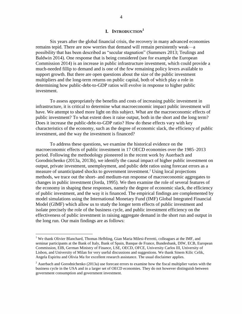
I. INTRODUCTION1

Six years after the global financial crisis, the recovery in many advanced economies

remains tepid. There are now worries that demand will remain persistently weak—a

possibility that has been described as “secular stagnation” (Summers 2013; Teulings and

Baldwin 2014). One response that is being considered (see for example the European

Commission 2014) is an increase in public infrastructure investment, which could provide a

much-needed fillip to demand and is one of the few remaining policy levers available to

support growth. But there are open questions about the size of the public investment

multipliers and the long-term returns on public capital, both of which play a role in

determining how public-debt-to-GDP ratios will evolve in response to higher public

investment.

To assess appropriately the benefits and costs of increasing public investment in

infrastructure, it is critical to determine what macroeconomic impact public investment will

have. We attempt to shed more light on this subject. What are the macroeconomic effects of

public investment? To what extent does it raise output, both in the short and the long term?

Does it increase the public-debt-to-GDP ratio? How do these effects vary with key

characteristics of the economy, such as the degree of economic slack, the efficiency of public

investment, and the way the investment is financed?

To address these questions, we examine the historical evidence on the

macroeconomic effects of public investment in 17 OECD economies over the 1985–2013

period. Following the methodology pioneered in the recent work by Auerbach and

Gorodnichenko (2013a, 2013b), we identify the causal impact of higher public investment on

output, private investment, unemployment, and public debt ratios using forecast errors as a

measure of unanticipated shocks to government investment.2 Using local projections

methods, we trace out the short- and medium-run response of macroeconomic aggregates to

changes in public investment (Jorda, 1995). We then examine the role of several features of

the economy in shaping these responses, namely the degree of economic slack, the efficiency

of public investment, and the way it is financed. The empirical findings are complemented by

model simulations using the International Monetary Fund (IMF) Global Integrated Financial

Model (GIMF) which allow us to study the longer term effects of public investment and

isolate precisely the role of the business cycle, and public investment efficiency on the

effectiveness of public investment in raising aggregate demand in the short run and output in

the long run. Our main findings are as follows:

1 We thank Olivier Blanchard, Thomas Helbling, Gian Maria Milesi-Ferretti, colleagues at the IMF, and

seminar participants at the Bank of Italy, Bank of Spain, Banque de France, Bundesbank, DIW, ECB, European

Commission, EIB, German Ministry of Finance, LSE, OECD, OFCE, University Carlos III, University of

Lisbon, and University of Milan for very useful discussions and suggestions. We thank Sinem Kilic Celik,

Angela Espiritu and Olivia Ma for excellent research assistance. The usual disclaimer applies.

2 Auerbach and Gorodnichenko (2013a) use forecast errors to examine how the fiscal multiplier varies with the

business cycle in the USA and in a larger set of OECD economies. They do not however distinguish between

government consumption and government investment.

5

Increased public investment raises output, both in the short term because of demand

effects and in the long term as a result of supply effects.

But these effects vary with a number of mediating factors, including (1) the degree of

economic slack and monetary accommodation, (2) the efficiency of public

investment, and (3) how public investment is financed.

When there is economic slack and monetary accommodation, demand effects are

stronger, and the public-debt-to-GDP ratio may actually decline.

An increase in public investment that is debt financed could have larger output effects

than one that is budget neutral, with both options delivering similar declines in the

public-debt-to-GDP ratio.

This paper contributes to several strands of literature. First, it reexamines the role of

infrastructure and public investment in economic development. A large body of literature has

focused on the optimal scale of public investment by estimating the long-term elasticity of

output to public and infrastructure capital using a production function approach (see Romp

and de Haan 2007; Straub 2011; and Bom and Ligthart 2014, for surveys of the literature).

Empirically, however, it is difficult to obtain estimates using this approach, which could be

given a causal interpretation. Unobservable factors may affect both economic performance

and government investment decisions, and the relationship between the two likely runs in

both directions. In contrast, our analysis adopts an empirical strategy that allows estimation

of both the short- and medium-term causal effects of public investment on a range of

macroeconomic variables. The paper also builds on the extensive literature on the

macroeconomic effects of fiscal policy and how these might be shaped by the state of the

business cycle and other factors (see, among others, Blanchard and Perotti 2002; Favero and

Giavazzi 2009; Romer and Romer 2010; Kraay 2012; Auerbach and

Gorodnichenko 2013a, 2013b; and Blanchard and Leigh 2013). Most of these papers do not

distinguish between the effects of government consumption and government investment;3 nor

do they examine the longer term effects of fiscal shocks. Finally, the paper contributes to the

recent literature that has used DSGE models to analyze the effects of government spending

shocks in a liquidity trap, including papers by Cogan et al (2010), Freedman et al (2010),

Erceg and Linde (2010a,b), Eggerston (2011), Woodford (2011), Christiano et al (2011), and

Coenen et al (2012).

The rest of the paper is organized as follows. Section II presents a stylized framework

for thinking about the macroeconomic effects of public investment. Section III presents the

empirical analysis used to assess the macroeconomic effect of public investment and

describes the data. Section IV presents the main findings and several robustness checks of the

empirical results, while Section V complements these with model simulations. Section VI

concludes summarizing the main findings and policy implications.

3 Eden and Kraay (2014) is a notable exception. Their paper examines the causal effect of public investment on

private investment and growth in a sample of low income countries.

6

II. THE MACROECONOMIC EFFECTS OF PUBLIC INVESTMENT: A STYLIZED FRAMEWORK

What are the macroeconomic effects of public investment? Following Delong and

Summers (2012), this section presents a highly stylized framework to assess the effect of

public investment on output and the debt-to-GDP ratio, and to evaluate the conditions under

which an increase in public investment may be self-financing.

An increase in public infrastructure investment affects the economy in two ways.

First, similar to other government spending, it boosts aggregate demand through the short-

term fiscal multiplier, whose magnitude may vary with the state of the economy (Auerbach

and Gorodnichenko, 2013a, 2013b). It may also crowd in private investment, given the

highly complementary nature of infrastructure services. The increase in government spending

will also affect the debt-to-GDP ratio, which may increase or decrease depending on the size

of the fiscal multiplier and on the elasticity of revenues to output .

More formally, as demonstrated in Delong and Summers (2012), in the short term

(one year), an increase in public investment as a share of potential GDP ( leads to a

change in the debt-to-potential GDP ratio ( ) given by

, (1)

in which is the fiscal multiplier and is the marginal tax rate.

Over time, there is also a supply-side effect of public infrastructure investment as the

productive capacity of the economy increases with the higher infrastructure capital stock.

The efficiency of investment is central to determining how large this supply-side effect will

be. Inefficiencies in the public investment process, such as poor project selection,

implementation, and monitoring, can result in only a fraction of public investment translating

into productive infrastructure, limiting the long-term output gains (Pritchett 2000;

Caselli 2005).

The extent to which increases in public capital can raise potential output is a key

factor in determining the evolution of the public-debt-to-GDP ratio over the medium and

long term. Over time, the increase in public investment will affect the debt-to-GDP ratio by

affecting its annual debt-financing burden, which is equal to the difference between the real

government borrowing rate (r) and the GDP growth rate (g) times the initial change in the

debt-to-GDP ratio:

(2)

Whether this additional financing burden will lead to an increase in the debt-to-GDP

ratio in the long term will depend on the parameters of equation (2) but also crucially on the

long-run elasticity of output to public capital, . In particular, in the long term, an increase in

public investment will lead to an increase in potential output (Y), which will generate long-

term future tax dividends:

(3)

7

in which is the long-term elasticity of output to public capital and is the initial output-to-

public capital ratio.4 Equations (2) and (3) imply together that if short-term multipliers and

the elasticity of output to public capital are sufficiently large, such that

then at the margin, an increase in public investment will be self-financing.

III. EMPIRICAL STRATEGY AND DATA

This rest of the paper examines whether the theoretical predictions regarding the

macroeconomic effects of public investment are borne out in the data, applying the statistical

approach used by Auerbach and Gorodnichenko (2013a, 2013b) and model simulations. To

identify the causal effect of public investment on output and the debt-to-GDP ratio, our

empirical approach isolates unanticipated changes in public investment as public investment

forecasts errors. Namely, the measure of government investment shocks is the difference

between the actual public investment and the public investment expected by analysts as of

October of the same year. This methodology overcomes two factors that often confound the

causal estimation of the effect of fiscal policy on economic performance.

First, using forecast errors eliminates the problem of “fiscal foresight” (see Forni and

Gambetti 2010; Leeper, Richter, and Walker 2012; Leeper, Walker, and Yang 2013; and Ben

Zeev and Pappa 2014). Agents receive news about changes in fiscal spending in advance and

they may alter their consumption and investment behavior well before the changes occur. An

econometrician who uses just the information contained in the change in actual public

investment would be relying on an information set that is smaller than that used by economic

agents, which could lead to inconsistent estimates of the effects of public investment.5 By

using forecast errors, the Auerbach and Gorodnichenko (2013a, 2013b) methodology

effectively aligns the economic agents’ and the econometrician’s information sets.

Second, using forecast errors minimizes the likelihood that the estimates capture the

potentially endogenous response of fiscal policy to the state of the economy. Even if public

investment shocks are unanticipated, they may still be in response to business cycle

conditions: for example, public projects may be stepped up if growth turns out to be

unexpectedly weak, or alternatively, they may be postponed if fiscal space is tight and

revenues surprise on the downside. For this to be a concern, however, such adjustments to

public investment need to happen within the same quarter news about the state of the

economy is received (i.e. between October and December), since all information about both

public investment and economic performance up until October are incorporated in the

4 For simplicity of formulation, the depreciation rate is assumed to be zero.

5 Leeper, Richter, and Walker (2012) demonstrate the potentially serious econometric problems that result from

fiscal foresight, showing that when agents foresee changes in fiscal policy, the resulting time series have

nonfundamental representations.

8

October forecasts. This is highly unlikely. Furthermore, we later demonstrate that our

findings are robust to purging the public investment shocks from forecast errors in growth.

Using these measures of unanticipated public investment shocks, we estimate two

econometric specifications. First we establish the impact of public investment shocks on real

GDP, the debt-to-GDP ratio, private investment as a share of GDP, and the unemployment

rate. We then examine whether the effects of public investment vary with the state of the

economy following a growing literature that explores the effect of fiscal policy during

recessions and expansions (see Auerbach and Gorodnichenko 2013a, 2013b; Blanchard and

Leigh 2013; IMF 2013; and the literature cited therein). We also investigate the role of public

investment efficiency and mode of financing in shaping the macroeconomic effects of

government investment.

The statistical method follows the approach proposed by Jordà (2005) to estimate

impulse-response functions using local projections. This approach has been advocated by

Stock and Watson (2007) and Auerbach and Gorodichencko (2013a), among others, as a

flexible alternative that does not impose the dynamic restrictions embedded in vector

autoregression (autoregressive-distributed lag) specifications and is particularly suited to

estimating nonlinearities in the dynamic response. The first regression specification is

estimated as follows:

(4)

in which y is the dependent variable (alternatively the log of output, the public-debt-to-GDP

ratio, the private investment-to-GDP ratio, and the unemployment rate); are country fixed

effects, included to control for all time-invariant differences across countries (such as in

countries’ growth rates); are time fixed effects, included to control for global shocks such

as shifts in oil prices or the global business cycle; and FE is the forecast error of public

investment as a share of GDP, computed as the difference between actual and forecast series.

Equation (4) is estimated for each k = 0, . . , 4. Impulse-response functions are computed

using the estimated coefficients , while the confidence bands associated with the estimated

impulse-response functions are obtained using the estimated standard errors of the

coefficients , based on clustered robust standard errors.

In the second specification, the response of the variable of interest is allowed to vary

with the state of the economy and with the degree of public investment efficiency. The

second regression specification is estimated as follows:

(5)

with

9

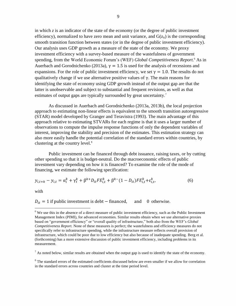
in which z is an indicator of the state of the economy (or the degree of public investment

efficiency), normalized to have zero mean and unit variance, and G(zit) is the corresponding

smooth transition function between states (or in the degree of public investment efficiency).

Our analysis uses GDP growth as a measure of the state of the economy. We proxy

investment efficiency with a survey-based measure of the wastefulness of government

spending, from the World Economic Forum’s (WEF) Global Competitiveness Report.6 As in

Auerbach and Gorodnichenko (2013a), is used for the analysis of recessions and

expansions. For the role of public investment efficiency, we set . The results do not

qualitatively change if we use alternative positive values of . The main reasons for

identifying the state of economy using GDP growth instead of the output gap are that the

latter is unobservable and subject to substantial and frequent revisions, as well as that

estimates of output gaps are typically surrounded by great uncertainty.7

As discussed in Auerbach and Gorodnichenko (2013a, 2013b), the local projection

approach to estimating non-linear effects is equivalent to the smooth transition autoregressive

(STAR) model developed by Granger and Teravistra (1993). The main advantage of this

approach relative to estimating STVARs for each regime is that it uses a larger number of

observations to compute the impulse response functions of only the dependent variables of

interest, improving the stability and precision of the estimates. This estimation strategy can

also more easily handle the potential correlation of the standard errors within countries, by

clustering at the country level.8

Public investment can be financed through debt issuance, raising taxes, or by cutting

other spending so that it is budget-neutral. Do the macroeconomic effects of public

investment vary depending on how it is financed? To examine the role of the mode of

financing, we estimate the following specification:

(6)

with

otherwise.

6 We use this in the absence of a direct measure of public investment efficiency, such as the Public Investment

Management Index (PIMI), for advanced economies. Similar results obtain when we use alternative proxies

based on “government efficiency” or “overall quality of infrastructure,” both also from the WEF’s Global

Competitiveness Report. None of these measures is perfect; the wastefulness and efficiency measures do not

specifically refer to infrastructure spending, while the infrastructure measure reflects overall provision of

infrastructure, which could be poor due to low efficiency but also because of inadequate spending. Berg et al.

(forthcoming) has a more extensive discussion of public investment efficiency, including problems in its

measurement.

7 As noted below, similar results are obtained when the output gap is used to identify the state of the economy.

8 The standard errors of the estimated coefficients discussed below are even smaller if we allow for correlation

in the standard errors across countries and cluster at the time period level.

10

The macroeconomic series used in the analysis come from the Organization for

Economic Co-operation and Development’s (OECD’s) Statistics and Projections database,

which covers an unbalanced sample of 17 OECD economies (Australia, Belgium, Canada,

Denmark, Finland, France, Germany, Iceland, Japan, Korea, Netherlands, New Zealand,

Norway, Sweden, Switzerland, United Kingdom, United States) over the period 1985–2013.

The forecasts of investment spending used in the analysis are those reported in the fall issue

of the OECD’s Economic Outlook for the same year (see Vogel 2007 and Lenain 2002 for an

assessment of OECD forecasts and a comparison with forecasts prepared by the private

sector). The size of the public investment shocks identified using this approach varies

between –4.6 and 1.2 percentage points of GDP, with an average (median) of about –0.3

(–0.1) percentage point of GDP.

IV. EMPIRICAL FINDINGS

A. Baseline results

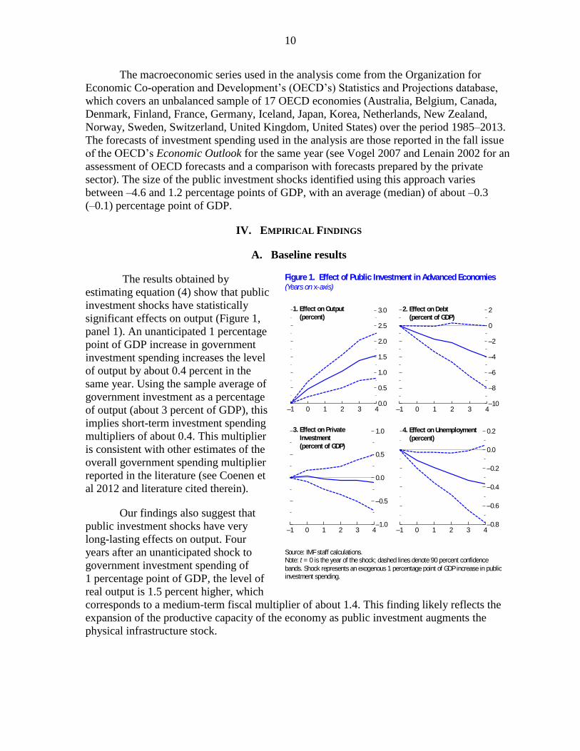
The results obtained by

estimating equation (4) show that public

investment shocks have statistically

significant effects on output (Figure 1,

panel 1). An unanticipated 1 percentage

point of GDP increase in government

investment spending increases the level

of output by about 0.4 percent in the

same year. Using the sample average of

government investment as a percentage

of output (about 3 percent of GDP), this

implies short-term investment spending

multipliers of about 0.4. This multiplier

is consistent with other estimates of the

overall government spending multiplier

reported in the literature (see Coenen et

al 2012 and literature cited therein).

Our findings also suggest that

public investment shocks have very

long-lasting effects on output. Four

years after an unanticipated shock to

government investment spending of

1 percentage point of GDP, the level of

real output is 1.5 percent higher, which

corresponds to a medium-term fiscal multiplier of about 1.4. This finding likely reflects the

expansion of the productive capacity of the economy as public investment augments the

physical infrastructure stock.

0.0

0.5

1.0

1.5

2.0

2.5

3.0

–1 0 1 2 3 4

Figure 1. Effect of Public Investment in Advanced Economies(Years on x-axis)

1. Effect on Output

(percent)

Source: IMF staff calculations.Note: t = 0 is the year of the shock; dashed lines denote 90 percent confidence

bands. Shock represents an exogenous 1 percentage point of GDP increase in public investment spending.

–10

–8

–6

–4

–2

0

2

–1 0 1 2 3 4

2. Effect on Debt

(percent of GDP)

–1.0

–0.5

0.0

0.5

1.0

–1 0 1 2 3 4

3. Effect on Private

Investment

(percent of GDP)

–0.8

–0.6

–0.4

–0.2

0.0

0.2

–1 0 1 2 3 4

4. Effect on Unemployment

(percent)

11

Perhaps surprisingly, higher public investment spending is not associated with an

increase in the debt-to-GDP ratio. The point estimates in panel 2 of the figure show that

higher public investment is typically followed by a reduction in the debt-to-GDP ratio, both

in the short term (by about 0.9 percentage point of GDP) and in the medium term (by about

4 percentage points of GDP), but the

decline in debt is statistically significant

only in the short term. On average, in the

advanced economies in our sample, the

boost to GDP from higher government

investment spending seems to be larger

than the public debt taken to finance it.

There is no statistically significant

effect on private investment as a share of

GDP (panel 3). This result suggests the

crowding in of private investment, as the

level of private investment rises in tandem

with the higher GDP as a result of the

increase in public investment. Finally, an

increase in public investment is found to

reduce the unemployment rate by about

0.11 percent in the very short term and by

about 0.35 percent over the medium term

(panel 4).

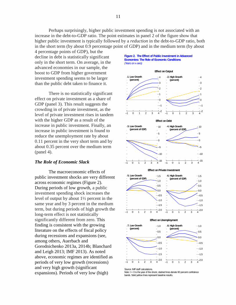
The Role of Economic Slack

The macroeconomic effects of

public investment shocks are very different

across economic regimes (Figure 2).

During periods of low growth, a public

investment spending shock increases the

level of output by about 1½ percent in the

same year and by 3 percent in the medium

term, but during periods of high growth the

long-term effect is not statistically

significantly different from zero. This

finding is consistent with the growing

literature on the effects of fiscal policy

during recessions and expansions (see,

among others, Auerbach and

Gorodnichenko 2013a, 2014b; Blanchard

and Leigh 2013; IMF 2013). As noted

above, economic regimes are identified as

periods of very low growth (recessions)

and very high growth (significant

expansions). Periods of very low (high)

Figure 2. The Effect of Public Investment in Advanced

Economies: The Role of Economic Conditions(Years on x-axis)

1. Low Growth

(percent)

Source: IMF staff calculations.Note: t = 0 is the year of the shock; dashed lines denote 90 percent confidence

bands. Solid yellow lines represent baseline results.

–2

–1

0

1

2

3

4

–1 0 1 2 3 4

2. High Growth

(percent)

–15

–10

–5

0

5

10

–1 0 1 2 3 4

3. Low Growth

(percent of GDP)

–15

–10

–5

0

5

10

–1 0 1 2 3 4

4. High Growth

(percent of GDP)

Effect on Output

Effect on Debt

–2.0

–1.5

–1.0

–0.5

0.0

0.5

1.0

1.5

–1 0 1 2 3 4

5. Low Growth

(percent of GDP)

–2.0

–1.5

–1.0

–0.5

0.0

0.5

1.0

1.5

–1 0 1 2 3 4

6. High Growth

(percent of GDP)

Effect on Private Investment

–2

–1

0

1

2

3

4

–1 0 1 2 3 4

–2.0

–1.5

–1.0

–0.5

0.0

0.5

1.0

–1 0 1 2 3 4

7. Low Growth

(percent)

–2.0

–1.5

–1.0

–0.5

0.0

0.5

1.0

–1 0 1 2 3 4

8. High Growth

(percent)

Effect on Unemployment

12

growth identified also correspond to periods of large negative (positive) output gaps: during

periods of very low (high) growth, the output gap varies between –0.4 and –7.2 (–1.1 and

8.5) percent of potential output, with an average output gap of –3.7 (3.5) percent. Using the

output gap instead of growth rates to identify

economic regimes gives qualitatively similar

results. In particular, during periods of large

negative output gaps, the short-term multiplier

is 0.6 and is statistically significant, but when

output gaps are large and positive, the output

effect of public investment is 0.2 and not

statistically significant.

Public investment shocks also bring

about a reduction in the public-debt-to-GDP

ratio during periods of low growth because of

the much bigger boost in output. During

periods of high growth, the point estimates

suggest a rise in public debt, though the wide

confidence intervals imply that the increase is

not statistically significantly different from

zero. The effects on private investment also

differ based on the state of the economy.

During low-growth periods, the increase in

private investment outpaces the increase in

GDP in the first few years, leading to a rise in

private investment as a share of GDP. But

during high-growth periods the opposite

happens, suggesting the possibility of

crowding out when there is less slack in the

economy. Finally, public investment shocks

reduce unemployment significantly during

low growth periods, by about half

a percentage point in the first year and by

¾ percentage point in the medium term, but

do not have a material effect on

unemployment rates during high-growth

periods.

The Role of Investment Efficiency

The macroeconomic effects of public

investment shocks are also substantially

stronger in countries with a high degree of

public investment efficiency, both in the short

–4

–3

–2

–1

0

1

2

3

4

5

6

–1 0 1 2 3 4

Figure 3. The Effect of Public Investment in Advanced

Economies: The Role of Efficiency(Years on x-axis)

1. High Efficiency

(percent)

Source: IMF staff calculations.Note: t = 0 is the year of the shock; dashed lines denote 90 percent confidence

bands. Solid yellow lines represent baseline results.

–4

–3

–2

–1

0

1

2

3

4

5

6

–1 0 1 2 3 4

2. Low Efficiency

(percent)

–35

–25

–15

–5

5

15

25

–1 0 1 2 3 4

3. High Efficiency

(percent of GDP)

–35

–25

–15

–5

5

15

25

–1 0 1 2 3 4

4. Low Efficiency

(percent of GDP)

Effect on Output

Effect on Debt

–4

–2

0

2

4

–1 0 1 2 3 4

5. High Efficiency

(percent of GDP)

Effect on Private Investment

–3.0

–2.0

–1.0

0.0

1.0

2.0

3.0

–1 0 1 2 3 4

7. High Efficiency

(percent)

–3.0

–2.0

–1.0

0.0

1.0

2.0

3.0

–1 0 1 2 3 4

8. Low Efficiency

(percent)

Effect on Unemployment

–4

–2

0

2

4

–1 0 1 2 3 4

6. Low Efficiency

(percent of GDP)

13

and in the medium term (Figure 3).9 In countries with high efficiency of public investment, a

public investment spending shock increases the level of output by about 0.8 percent in the

same year and by 2.6 percent four years after the shock. But in countries with low efficiency

of public investment, the output effect is about 0.2 percent in the same year and about

0.7 percent in the medium term. As a result, although public investment shocks are found to

lead to a significant medium-term reduction in the debt-to-GDP ratio in countries with high

public investment efficiency, they tend to increase the debt-to-GDP ratio (albeit not in a

statistically significant manner) in countries with low public investment efficiency. There is a

greater boost to private investment when public investment efficiency is high, whereas

private investment as a share of GDP falls when public investment efficiency is low. Finally,

the effects on unemployment reduction are larger in countries with a high level of investment

efficiency. No statistically significant correlation is found between the measure of investment

spending shocks used here and the degree of investment efficiency. This suggests that the

result that macroeconomic effects are larger in countries with higher investment efficiency is

not driven by the fact that investment spending shocks tend to occur more frequently and to

be larger in countries with higher degrees of public investment efficiency.10

The Role of Financing: Debt-financed vs. Budget-neutral Public Investment

9 Berg et al. (forthcoming) reconsider the macroeconomic implications of investment efficiency, noting that

countries with lower efficiency of public investment would tend to have lower capital stock, which would push

up public capital’s rates of return. In our analysis, this channel is likely subdued as we focus on a set of

advanced economies, with relatively little variation in the public capital stock.

10 In particular, the correlation between investment spending shocks and the degree of efficiency is –0.11.

14

The macroeconomic effects of public investment also vary depending on how it is

financed. Government projects financed through debt issuance have stronger expansionary

effects than budget-neutral projects that are financed by raising taxes or cutting other

spending. Budget-neutral public investment shocks are identified in the data as those in

which the difference between the shocks to other components of the government budget and

public investment shocks is greater than or equal to zero. We find that the output effects of

public investment tend to be larger when public investment shocks are debt-financed than

when they are budget-neutral (Figure 4). In particular, although a debt-financed public

investment shock of 1 percentage point of GDP increases the level of output by about

0.9 percent in the same year and by 2.9 percent four years after the shock, the short- and

medium-term output effects of a budget-neutral public investment shock are not statistically

significantly different from zero. The larger short- and medium-term output multipliers for

debt-financed shocks imply that the reduction in the debt-to-GDP ratio is similar in the two

types of shocks. The short-term effects on private investment are similar to those in the

baseline regardless of how public investment is financed, but private investment is boosted as

a share of GDP in the medium-term when public investment is debt-financed, possibly

because of the larger output multipliers. Finally, and in line with the differing effects on

output, the effects of public investment on unemployment are bigger when it is debt-financed

than when it is budget-neutral.

It is possible that increasing debt-financed public investment in countries where debt

is already high may increase sovereign risk and financing costs if the productivity of the

investment is in doubt (e.g., because of poor project selection or implementation),

exacerbating debt sustainability concerns. We thus examine whether public investment

shocks are associated with subsequent changes in real interest rates. Within the sample of

17 advanced economies employed in the estimation, the empirical evidence suggests that

historically, debt-financed public investment shocks have not led to increases in funding

costs, as proxied by sovereign real interest rates (Figure 5, panels 1 and 2).

15

Moreover, an examination of whether the effects of public investment shocks on debt

and output depend on the initial level of public debt yields no evidence that the effects of

public investment differ materially according to the initial public-debt-to-GDP ratio

Figure 4. The Effect of Public Investment in Advanced

Economies: The Role of Mode of Financing(Years on x-axis)

1. Debt Financed

(percent)

Source: IMF staff calculations.Note: t = 0 is the year of the shock; dashed lines denote 90 percent confidence

bands. Solid yellow lines represent baseline results.

–2

–1

0

1

2

3

4

5

6

–1 0 1 2 3 4

2. Budget Neutral

(percent)

–35

–25

–15

–5

5

15

25

–1 0 1 2 3 4

3. Debt Financed

(percent of GDP)

–35

–25

–15

–5

5

15

25

–1 0 1 2 3 4

4. Budget Neutral

(percent of GDP)

Effect on Output

Effect on Debt

–2

–1

0

1

2

3

4

5

6

–1 0 1 2 3 4

–2

–1

0

1

2

3

4

–1 0 1 2 3 4

5. Debt Financed

(percent of GDP)

–2

–1

0

1

2

3

4

–1 0 1 2 3 4

6. Debt Neutral

(percent of GDP)

Effect on Private Investment

–3.0

–2.5

–2.0

–1.5

–1.0

–0.5

0.0

0.5

1.0

–1 0 1 2 3 4

7. Debt Financed

(percent)

–3.0

–2.5

–2.0

–1.5

–1.0

–0.5

0.0

0.5

1.0

–1 0 1 2 3 4

8. Debt Neutral

(percent)

Effect on Unemployment

–1.5

–1.0

–0.5

0.0

0.5

1.0

1.5

–1 0 1 2 3 4

Figure 5. Effect of Public Investment in Advanced Economies:

The Role of Mode of Financing(Percent; years on x-axis)

1. Debt Financed

Source: IMF staff calculations.Note: t = 0 is the year of the shock; dashed lines denote 90 percent confidence

bands. Solid yellow lines represent baseline results.

–1.5

–1.0

–0.5

0.0

0.5

1.0

1.5

–1 0 1 2 3 4

2. Budget Neutral

3. Low Initial Debt

–1

0

1

2

3

4

5

–1 0 1 2 3 4

4. High Initial Debt

Effect on Real Interest Rate

Effect on Output

–1

0

1

2

3

4

5

–1 0 1 2 3 4

5. Debt < 100% of GDP

–1

1

2

3

4

5

–1 0 1 2 3 4

6. Debt > 100% of GDP

–1

0

1

2

3

4

5

–1 0 1 2 3 4

16

(Figure 5, panels 3 and 4). This may, in principle, reflect the fact that debt-to-GDP ratios in

advanced economies were moderate during most of the sample period. However, even when

we focus on country-periods of very high-debt (namely, when the debt-to-GDP ratio exceeds

100 percent of GDP – the 90th

percentile of the debt-to-GDP distribution in the sample), we

do not find any evidence of non-linear effects of the initial level of public debt (Figure 5,

panels 5 and 6).

B. Robustness Checks

Our findings are robust to alternative measures of public investment shocks,

estimation periods, and country samples. As a first robustness check, we use the forecasts of

the spring issue of the same year and the fall issue of the previous year instead of the October

forecast to compute government investment forecast errors. The results in columns 2 and 3 of

Table 1 show that the response functions of real output are almost identical and not

statistically significantly different from that reported in the baseline (Table 1, column 1).

As an additional robustness check, we assess whether the effects of public investment

on output have changed over time. The results show that this is not the case. There has been

no statistically significant change in the public investment multiplier over time in our sample

of advanced economies, even though the point estimates of the output effect of public

investment are somewhat larger in the post-2000 period.

Baseline

April

forecast

Previous

October

Forecast Pre 2000 Post 2000 Growth

Demand

components 1/

Positive

Shocks

Negative

Shocks

Trimmed

top and

bottom 1%

of shocks

(1) (2) (3) (4) (5) (6) (7) (8) (9) (10)

Impact of public investment shock on output at k=

0 0.457 0.264 0.332 0.401 0.581 0.418 0.502 1.013 0.316 0.466

(0.147) (0.160) (0.118) (0.198) (0.209) (0.147) (0.143) (0.447) (0.181) (0.138)

1 0.755 0.581 0.697 0.582 0.948 0.702 0.844 1.240 0.584 0.740

(0.238) (0.216) (0.216) (0.301) (0.387) (0.241) (0.264) (0.619) (0.309) (0.232)

2 1.035 0.966 1.004 0.753 1.223 0.993 1.241 1.576 0.888 1.058

(0.322) (0.270) (0.288) (0.414) (0.489) (0.323) (0.339) (0.763) (0.431) (0.302)

3 1.389 1.099 1.124 1.036 1.569 1.354 1.625 1.706 1.242 1.492

(0.394) (0.349) (0.330) (0.526) (0.575) (0.393) (0.405) (0.754) (0.547) (0.358)

4 1.539 1.318 1.219 1.135 1.642 1.507 1.864 1.459 1.393 1.747

(0.441) (0.402) (0.383) (0.590) (0.796) (0.439) (0.489) (0.715) (0.617) (0.405)

1/ Demand components include private consumption, investment and government consumption.

Purging forecast errors for forecast

errors in:

Note: k=0 is the year of the public investment shock, measured by the public investment forecast error. Standard errors (in parentheses below the

ceofficients) are corrected for heteroskedasticity and clustered at the country level. Sample includes 17 OECD economies for the 1985-2013 period. All

regressions include a full set of country and year fixed effects.

Table 1. Effect of Public Investment on Output in Advanced Economies: Robustness

17

A problem in the identification of public investment shocks is that they may be

endogenous to output growth surprises. Indeed, whereas automatic stabilizers operate mostly

via revenues and social spending, discretionary public investment spending can occur in

response to output conditions. To ensure that our findings do not capture this potential

reverse relationship between output and investment, we separate public investment shocks

from output growth innovations.11 The results obtained by separating public investment

shocks from output growth innovations are almost identical and not statistically significantly

different from those reported in the baseline (Table 1, column 6).

Another possible problem in identifying public investment shocks is a potential

systematic bias in the forecasts concerning economic variables other than public investment,

with the result that the forecast errors for public investment are correlated with those for

other macroeconomic variables. To address this concern, we regress the measure of public

investment shocks on the forecast errors of other components of government spending,

private investment, and private consumption, and use the residuals from this regression as

our measure of public investment shocks. The results, presented in column 7 of Table 1,

show that the response functions of output are almost identical and not statistically

significantly different from that reported in the baseline.

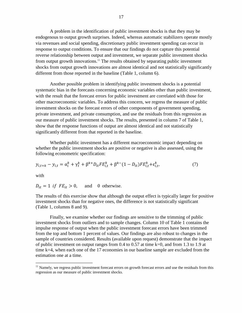
Whether public investment has a different macroeconomic impact depending on

whether the public investment shocks are positive or negative is also assessed, using the

following econometric specification:

(7)

with

otherwise.

The results of this exercise show that although the output effect is typically larger for positive

investment shocks than for negative ones, the difference is not statistically significant

(Table 1, columns 8 and 9).

Finally, we examine whether our findings are sensitive to the trimming of public

investment shocks from outliers and to sample changes. Column 10 of Table 1 contains the

impulse response of output when the public investment forecast errors have been trimmed

from the top and bottom 1 percent of values. Our findings are also robust to changes in the

sample of countries considered. Results (available upon request) demonstrate that the impact

of public investment on output ranges from 0.4 to 0.57 at time k=0, and from 1.3 to 1.9 at

time k=4, when each one of the 17 economies in our baseline sample are excluded from the

estimation one at a time.

11

Namely, we regress public investment forecast errors on growth forecast errors and use the residuals from this

regression as our measure of public investment shocks.

18

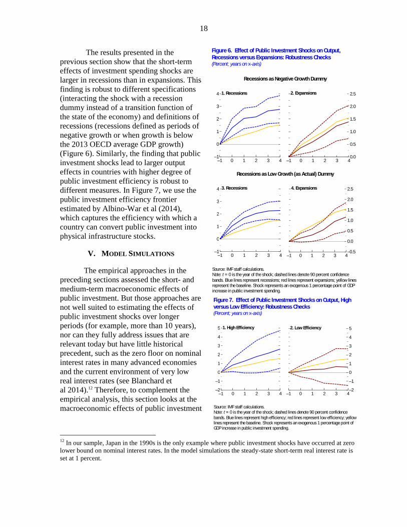
The results presented in the

previous section show that the short-term

effects of investment spending shocks are

larger in recessions than in expansions. This

finding is robust to different specifications

(interacting the shock with a recession

dummy instead of a transition function of

the state of the economy) and definitions of

recessions (recessions defined as periods of

negative growth or when growth is below

the 2013 OECD average GDP growth)

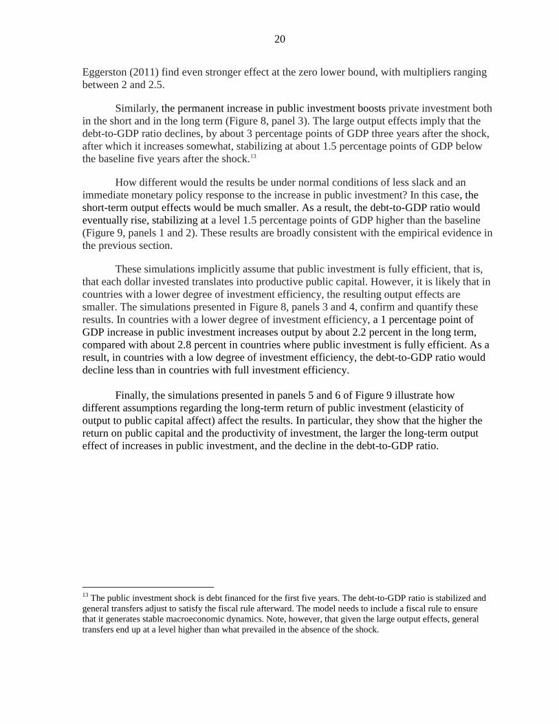
(Figure 6). Similarly, the finding that public

investment shocks lead to larger output

effects in countries with higher degree of

public investment efficiency is robust to

different measures. In Figure 7, we use the

public investment efficiency frontier

estimated by Albino-War et al (2014),

which captures the efficiency with which a

country can convert public investment into

physical infrastructure stocks.

V. MODEL SIMULATIONS

The empirical approaches in the

preceding sections assessed the short- and

medium-term macroeconomic effects of

public investment. But those approaches are

not well suited to estimating the effects of

public investment shocks over longer

periods (for example, more than 10 years),

nor can they fully address issues that are

relevant today but have little historical

precedent, such as the zero floor on nominal

interest rates in many advanced economies

and the current environment of very low

real interest rates (see Blanchard et

al 2014).12 Therefore, to complement the

empirical analysis, this section looks at the

macroeconomic effects of public investment

12

In our sample, Japan in the 1990s is the only example where public investment shocks have occurred at zero

lower bound on nominal interest rates. In the model simulations the steady-state short-term real interest rate is

set at 1 percent.

–2

–1

0

1

2

3

4

5

–1 0 1 2 3 4

Figure 7. Effect of Public Investment Shocks on Output, High

versus Low Efficiency: Robustness Checks(Percent; years on x-axis)

Source: IMF staff calculations.Note: t = 0 is the year of the shock; dashed lines denote 90 percent confidence

bands. Blue lines represent high efficiency; red lines represent low efficiency; yellow lines represent the baseline. Shock represents an exogenous 1 percentage point of GDP increase in public investment spending.

–2

–1

0

1

2

3

4

5

–1 0 1 2 3 4

1. High Efficiency 2. Low Efficiency

–1

0

1

2

3

4

–1 0 1 2 3 4

–0.5

0.0

0.5

1.0

1.5

2.0

2.5

–1 0 1 2 3 4

0.0

0.5

1.0

1.5

2.0

2.5

–1 0 1 2 3 4

Figure 6. Effect of Public Investment Shocks on Output,

Recessions versus Expansions: Robustness Checks(Percent; years on x-axis)

Source: IMF staff calculations.Note: t = 0 is the year of the shock; dashed lines denote 90 percent confidence

bands. Blue lines represent recessions; red lines represent expansions; yellow lines represent the baseline. Shock represents an exogenous 1 percentage point of GDP increase in public investment spending.

1. Recessions 2. Expansions

Recessions as Negative Growth Dummy

–1

0

1

2

3

4

–1 0 1 2 3 4

3. Recessions 4. Expansions

Recessions as Low Growth (as Actual) Dummy

19

shocks using a dynamic stochastic general-equilibrium model.

The analysis uses the IMF’s Globally Integrated Monetary and Fiscal model (see

Kumhof and Laxton 2007; Kumhof, Muir, and Mursula 2010; Coenen and others 2012; for a

detailed description of the model). The main advantage of using such a structural model is

that public investment shocks are strictly exogenous and no identification assumptions are

needed. Moreover, the model presents some attractive features particularly relevant for the

assessment of the impact of fiscal shocks. First, it has a highly detailed fiscal policy block.

Second, it incorporates some empirically relevant channels that shape the transmission of

fiscal shocks (for example, it specifies that a significant share of households is liquidity

constrained). Third, the model captures the effect of automatic stabilizers on both the tax and

spending side.

A critical input in the model-based analysis is the elasticity of output to public capital.

There is now a substantial literature, triggered by the seminal contributions of Aschauer

(1989), that estimates the long-term elasticity of output to public capital. A cursory reading

of the literature reveals estimates ranging widely, from large and positive to slightly negative.

However, a recent meta-analysis by Bom and Ligthart (2014) of 68 of these studies shows

that much of the variation in estimates can be attributed to differences in research design,

including how public infrastructure capital is defined, what output measure is used, whether

capital is installed at the national level or by state and local governments, the econometric

specification and sample coverage, and whether endogeneity and nonstationarity are properly

addressed. Controlling for these factors, Bom and Ligthart come up with a much narrower

range for the estimated output elasticity of public capital. In particular, they suggest that the

elasticity of output with respect to core infrastructure installed by a national government is

0.17. This is the estimated elasticity that is assumed in the baseline simulations.

Since the global financial crisis, policy rates in the largest advanced economies have

been near zero and are expected to remain at this level in the near term because of still-large

output gaps. The effects of public investment shocks under these conditions are examined

through a simulation of the macroeconomic response of output, the public-debt-to-GDP ratio,

and private investment to a 1 percent of GDP increase in public investment, assuming that

monetary policy rates stay close to zero for two years. There are two main reasons to assume

that policy rates stay near zero for two years. First, such an assumption is in line with market

expectations about policy rates for most large advanced economies. Second, in the model, the

only way the central bank can stabilize output and inflation is by cutting nominal interest

rates. When the option of cutting interest rates is removed for a longer period—for example,

three or more years—the model generates unstable macroeconomic dynamics, which

complicates the computation of simulation results.

The results of this simulation suggest that a 1 percent of GDP permanent increase in

public investment increases output by about 2 percent in the same year. Output declines in

the third year after the shock as monetary policy normalizes, then increases to 2.5 percent

over the long term because of the resulting higher stock of public capital (Figure 8, panel 1).

These results are consistent with recent papers that have used theoretical models to analyze

the effect of fiscal stimulus in a liquidity trap. Hall (2009) finds a short- term output

multiplies close to 1.7 at a zero nominal interest rate. Christiano et al (2011) and

20

Eggerston (2011) find even stronger effect at the zero lower bound, with multipliers ranging

between 2 and 2.5.

Similarly, the permanent increase in public investment boosts private investment both

in the short and in the long term (Figure 8, panel 3). The large output effects imply that the

debt-to-GDP ratio declines, by about 3 percentage points of GDP three years after the shock,

after which it increases somewhat, stabilizing at about 1.5 percentage points of GDP below

the baseline five years after the shock.13

How different would the results be under normal conditions of less slack and an

immediate monetary policy response to the increase in public investment? In this case, the

short-term output effects would be much smaller. As a result, the debt-to-GDP ratio would

eventually rise, stabilizing at a level 1.5 percentage points of GDP higher than the baseline

(Figure 9, panels 1 and 2). These results are broadly consistent with the empirical evidence in

the previous section.

These simulations implicitly assume that public investment is fully efficient, that is,

that each dollar invested translates into productive public capital. However, it is likely that in

countries with a lower degree of investment efficiency, the resulting output effects are

smaller. The simulations presented in Figure 8, panels 3 and 4, confirm and quantify these

results. In countries with a lower degree of investment efficiency, a 1 percentage point of

GDP increase in public investment increases output by about 2.2 percent in the long term,

compared with about 2.8 percent in countries where public investment is fully efficient. As a

result, in countries with a low degree of investment efficiency, the debt-to-GDP ratio would

decline less than in countries with full investment efficiency.

Finally, the simulations presented in panels 5 and 6 of Figure 9 illustrate how

different assumptions regarding the long-term return of public investment (elasticity of

output to public capital affect) affect the results. In particular, they show that the higher the

return on public capital and the productivity of investment, the larger the long-term output

effect of increases in public investment, and the decline in the debt-to-GDP ratio.

13

The public investment shock is debt financed for the first five years. The debt-to-GDP ratio is stabilized and

general transfers adjust to satisfy the fiscal rule afterward. The model needs to include a fiscal rule to ensure

that it generates stable macroeconomic dynamics. Note, however, that given the large output effects, general

transfers end up at a level higher than what prevailed in the absence of the shock.

21

0.0

0.5

1.0

1.5

2.0

2.5

3.0

2013 14 15 16 17 18 19 20 21 22 23

Source: IMF staff estimates.Note: Shock represents an exogenous 1 percentage point of GDP increase in public investment spending.

Figure 8. Model Simulations: Effect of Public Investment in

Advanced Economies in the Current Scenario

1. Output

(percent deviation from baseline)

–4

–3

–2

–1

0

1

2013 14 15 16 17 18 19 20 21 22 23

2. Debt

(percentage-point-of-GDP deviation from baseline)

0.0

0.5

1.0

1.5

2.0

2.5

3.0

3.5

4.0

2013 14 15 16 17 18 19 20 21 22 23

3. Private Investment

(percent deviation from baseline)

–5

–4

–3

–2

–1

0

1

2

2013 15 17 19 21 23

–4

–2

0

2

4

2013 15 17 19 21 230

1

2

3

4

2013 15 17 19 21 23

Source: IMF staff estimates.Note: Shock represents an exogenous 1 percentage point of GDP increase inpublic investment spending.

Figure 9. Model Simulations: Effect of Public Investment in

Advanced Economies: The Role of Monetary Policy, Efficiency,

and Return on Public Capital

1. Effect on Output

(percent deviation from

baseline)

2. Effect on Debt

(percentage-point-of-GDP

deviation from baseline)

Monetary Policy

Monetary policy accommodates Monetary policy does not accommodate

0

1

2

3

4

2013 15 17 19 21 23

3. Effect on Output

(percent deviation from

baseline)

4. Effect on Debt

(percentage-point-of-GDP

deviation from baseline)

EfficiencyHigh efficiency Low efficiency

–5

–4

–3

–2

–1

0

1

2

2013 15 17 19 21 230

1

2

3

4

2013 15 17 19 21 23

5. Effect on Output

(percent deviation from

baseline)

6. Effect on Debt

(percentage-point-of-GDP

deviation from baseline)

Return on Public CapitalBaseline Low return High return

22

VI. CONCLUSIONS AND POLICY IMPLICATIONS

We examine the macroeconomic impact of increased public investment, and find that

such investment raises output in both the short and long term, crowds in private investment,

and reduces unemployment, with limited effect on the public debt ratio. We also find that

these effects vary with a number of mediating factors. The effects of public investment are

particularly strong when there is slack in the economy and monetary accommodation. In such

cases, the boost to output from higher government investment may exceed the debt issued to

finance the investment. Government projects are more effective in boosting output in

countries with higher efficiency of public investment. Finally, the mode of financing

investment matters. We find suggestive evidence that debt-financed projects have larger

expansionary effects than budget-neutral investments financed by raising taxes or cutting

other government spending.

Our findings suggest that for economies with clearly identified infrastructure needs

and efficient public investment processes and where there is economic slack and monetary

accommodation, there is a strong case for increasing public infrastructure investment.

Moreover, evidence suggests that increasing public infrastructure investment will be

particularly effective in providing a fillip to aggregate demand and expanding productive

capacity in the long run, without raising the debt-to-GDP ratio, if it is debt financed.

Finally, our results show how critical increasing investment efficiency is to mitigating

the possible trade-off between higher output and higher public-debt-to-GDP ratios. Thus a

key priority in many economies, particularly in those with relatively low efficiency of public

investment, should be to raise the quality of infrastructure investment by improving the

public investment process.

23

References

Albino-War, Maria, Svetlana Cerovic, Juan Carlos Flores, Francesco Grigoli, Javier Kapsoli,

Haonan Qu, Yahia Said, and others. 2014. “Making the Most of Public

Investment in Oil-Exporting Countries.” Staff Discussion Note 14/10,

International Monetary Fund, Washington.

Aschauer, David Alan. 1989. “Is Public Expenditure Productive?” Journal of Monetary

Economics 23 (2): 177–200.

Auerbach, Alan, and Yuriy Gorodnichenko. 2013a. “Fiscal Multipliers in Recession and

Expansion.” In Fiscal Policy After the Financial Crisis, eds. Alberto Alesina

and Francesco Giavazzi, NBER Books, National Bureau of Economic

Research, Inc., Cambridge, Massachusetts.

———. 2013b. “Measuring the Output Responses to Fiscal Policy.” American Economic

Journal: Economic Policy 4 (2): 1–27.

———. 2014. “Fiscal Multipliers in Japan.” NBER Working Paper 19911, National Bureau

of Economic Research, Cambridge, Massachusetts.

Ben Zeev, Nadav, and Evi Pappa. 2014. “Chronicle of a War Foretold: The Macroeconomic

Effects of Anticipated Defense Spending Shocks.” CEPR Discussion Paper

9948, Centre for Economic Policy Research, London.

Berg, Andrew, Ed Buffie, Catherine Pattillo, Rafael Portillo, Andrea Presbitero, and Luis-

Felipe Zanna. 2015. “Some Misconceptions about Public Investment

Efficiency and Growth.” IMF Working Paper, forthcoming.

Blanchard, Olivier J., Davide Furceri, and Andrea Pescatori. 2014. “A prolonged period of

low real interest rates?” Chapter 8 in Secular Stagnation: Facts, Causes and

Cures. Teulings, Coen, and Richard Baldwin, eds. London: Centre for

Economic Policy Research.

Blanchard, Olivier J., and Daniel Leigh. 2013. “Growth Forecast Errors and Fiscal

Multipliers.” American Economic Review 103 (3): 117–20.

Blanchard, Olivier J., and Roberto Perotti. 2002. “An Empirical Characterization of the

Dynamic Effects of Changes in Government Spending and Taxes on Output.”

Quarterly Journal of Economics 107 (4): 1329–68.

Bom, Pedro R., and Jenny E. Ligthart. 2014. “What Have We Learned from Three Decades

of Research on the Productivity of Public Capital?” Journal of Economic

Surveys 28 (5): 889–916.

Caselli, Francesco. 2005. “Accounting for Cross-Country Income Differences.” NBER

Working Paper 10828, National Bureau of Economic Research, Cambridge,

Massachusetts.

24

Christiano, Lawrence, Martin Eichenbaum, and Sergio Rebelo. 2011. “When Is the

Government Spending Multiplier Large?” Journal of Political Economy,

119(1): 78–121.

Coenen, Günter, Christopher J. Erceg, Charles Freedman, Davide Furceri, Michael Kumhof,

René Lalonde, Douglas Laxton, and others. 2012. “Effects of Fiscal Stimulus

in Structural Models.” American Economic Journal: Macroeconomics 4 (1):

22–68.

Cogan, John F., Tobias Cwik, John B. Taylor, and Volker Wieland. 2010. “New Keynesian

versus Old Keynesian Government Spending Multipliers.” Journal of

Economic Dynamics and Control 34(3): 281–295.

Delong, J. Bradford, and Lawrence H. Summers. 2012. “Fiscal Policy in a Depressed

Economy.” Brookings Papers on Economic Activity 44 (1): 233–97.

Eden, Maya, and Aart Kraay. 2014. “Crowding In and the Returns to Government

Investment in Low-Income Countries.” World Bank Policy Research Working

Paper 6781, World Bank, Washington.

Eggertsson, Gauti B. 2011. “What Fiscal Policy is Effective at Zero Interest Rates?” NBER

Macroeconomics Annual 2010, Vol. 25, ed. Daron Acemoglu and Michael

Woodford, 59–112. Chicago: University of Chicago Press.

Erceg Christopher J., and Jesper Lindé. 2010a. “Is There a Fiscal Free Lunch in a Liquidity

Trap?” Board of Governors of the Federal Reserve System, International

Finance Discussion Paper 1003.

Erceg, Christopher J., and Jesper Lindé. 2010b. “Asymmetric Shocks in a Currency Union

With Monetary and Fiscal Handcuffs.” NBER National Seminar on

Macroeconomics 2010. Vol. 7, ed. Richard Clarida, and Francesco Giavazzi,

95–135, Chicago: University of Chicago Press.

European Commission. 2014. “An Investment Plan for Europe.”

http://ec.europa.eu/priorities/jobs-growth-investment/plan/index_en.htm.

Favero, Carlo, and Francesco Giavazzi. 2009. “How Large are the Effects of Tax Changes?”

NBER Working Paper 15303, National Bureau of Economic Research, Inc.

Cambridge, Massachusetts.

Freedman, Charles, Michael Kumhof, Douglas Laxton, Dirk Muir and Susanna

Mursula. 2010. “Global Effect of Fiscal Stimulus During the Crisis.” Journal

of Monetary Economics 57: 506–526.

Forni, Mario, and Luca Gambetti. 2010. “Fiscal Foresight and the Effects of Government

Spending.” CEPR Discussion Paper 7840, Centre for Economic Policy

Research, London.

25

Granger, Clive W. J., and Timo Terasvirta. 1993. Modelling Nonlinear Economic

Relationships. New York: Oxford University Press.

Hall, Robert E. 2009. “By How Much Does GDP Rise if the Government Buys More

Output?” NBER Working Paper 15496, National Bureau of Economic

Research, Cambridge, Massachusetts.

International Monetary Fund (IMF). 2013. “Reassessing the Role and Modalities of Fiscal

Policy in Advanced Economies.” IMF Policy Paper, Washington.

Jordà, Òscar. 2005. “Estimation and Inference of Impulse Responses by Local Projections.”

American Economic Review 95 (1): 161–82.

Kraay, Aart. 2012. “How Large Is the Government Spending Multiplier? Evidence from

World Bank Lending.” Quarterly Journal of Economics 127 (2): 829–87.

———. Forthcoming. “Government Spending Multipliers in Developing Countries:

Evidence from Lending by Official Creditors.” American Economic Journal:

Macroeconomics.

Kumhof, Michael, and Douglas Laxton. 2007. “A Party without a Hangover? On the Effects

of U.S. Government Deficits.” IMF Working Paper 07/202, International

Monetary Fund, Washington.

Kumhof, Michael, Dirk Muir, and Susanna Mursula. 2010. “The Global Integrated Monetary

and Fiscal Model (GIMF)—Theoretical Structure.” IMF Working Paper

10/34, International Monetary Fund, Washington.

Leeper, Eric M., Alexander W. Richter, and Todd B. Walker. 2012. “Quantitative Effects of

Fiscal Foresight.” American Economic Journal: Economic Policy 4 (2): 115–

44.

Leeper, Eric M., Todd B. Walker, and Shu-Chun S. Yang. 2013. “Fiscal Foresight and

Information Flows.” Econometrica 81 (3): 1115–45.

Lenain, Patrick. 2002. “What Is the Track Record of OECD Economic Projections?”

Organisation for Economic Co-operation and Development, Paris.

Pritchett, Lant. 2000. “The Tyranny of Concepts: CUDIE (Cumulated, Depreciated,

Investment Effort) Is Not Capital.” Journal of Economic Growth 5 (4): 361–

84.

Romer, Christina, and David Romer. 2010. “The Macroeconomic Effects of Tax Changes:

Estimates Based on a New Measure of Fiscal Shocks.” American Economic

Review, Vol. 100, No. 3, pp. 763–801.

Romp, Ward, and Jakob de Haan. 2007. “Public Capital and Economic Growth: A Critical

Survey.” Perspectiven der Wirtschaftspolitik 8 (S1): 6–52.

26

Stock, James H., and Mark W. Watson. 2007. “Why Has U.S. Inflation Become Harder to

Forecast?” Journal of Money, Credit and Banking 39 (S1): 3–33.

Straub, Stephane. 2011. “Infrastructure and Development: A Critical Appraisal of the Macro-

level Literature.” Journal of Development Studies 47 (5): 683–708.

Summers, Lawrence H. 2013. Remarks in honor of Stanley Fischer. Fourteenth Jacques

Polak Annual Research Conference, International Monetary Fund,

Washington, November 7–8.

Teulings, Coen, and Richard Baldwin, eds. 2014. Secular Stagnation: Facts, Causes and

Cures. London: Centre for Economic Policy Research.

Vogel, Lukas. 2007. “How Do the OECD Growth Projections for the G7 Economies

Perform? A Post-mortem.” OECD Working Paper 573, Organisation for

Economic Co-operation and Development, Paris.

Woodford, Michael. 2011. “Simple Analytics of the Government Expenditure Multiplier.”

American Economic Journal: Macroeconomics, 3(1): 1–35.