the macroeconomics of us consumer bankruptcy choice: chapter
TRANSCRIPT
FEDERAL
Ten Independen
WORKING PAPERSRESEARCH DEPARTMENT
WORKING PAPER NO. 03-14 THE MACROECONOMICS OF U.S. CONSUMER
BANKRUPTCY CHOICE: CHAPTER 7 OR CHAPTER 13?
Wenli Li Federal Reserve Bank of Philadelphia
Pierre-Daniel Sarte
Federal Reserve Bank of Richmond
September 2002
RESERVE BANK OF PHILADELPHIA
ce Mall, Philadelphia, PA 19106-1574• (215) 574-6428• www.phil.frb.org

Working Paper No. 03-14
The Macroeconomics of U.S. Consumer Bankruptcy Choice: Chapter 7 or Chapter 13?
Wenli Li* and Pierre-Daniel Sarte†‡
September 2002
________________
*Research Department, Federal Reserve Bank of Philadelphia. †Corresponding Author: Pierre-Daniel Sarte, Research Department, Federal Reserve Bank of Richmond, P.O. Box 27622, Richmond, VA 23261. e-mail: [email protected]. ‡The views expressed in this paper are those of the authors and do not necessarily reflect those of the Federal Reserve Bank of Philadelphia, the Federal Reserve Bank of Richmond, or the Federal Reserve System. We thank Kartik Athreya, Andreas Hornstein, Je. Lacker, John Walter, John Weinberg, as well as seminar participants at the Board of Governors, the Federal Reserve Bank of New York, the 2002 Midwest Macroeconomics Conference, and the 2002 North American Summer Meetings of the Econometric Society for their comments. Any errors are our own.
Abstract
Because of the recent surge in U.S. personal defaults, Congress is currently debating bankruptcy
reform legislation requiring a means test for Chapter 7 filers. This paper explores the effects of
such a reform in a model where, in contrast to previous work, bankruptcy options and production
are explicitly taken into account. Our findings indicate that means testing would not improve upon
current bankruptcy provisions and, at best, leaves aggregate filings, output, and welfare unchanged.
Put simply, given already existing provisions, the introduction of an efficient means test would not
bind. However, we do find that a tightening of existing bankruptcy laws, in the form of lower
Chapter 7 asset exemptions, can be welfare improving. Contrary to previous studies, the analysis
also suggests that eliminating bankruptcy entirely would cause significant declines in both output
and welfare.
JEL Classifications: D52; G18
Keywords: Chapter 7 and Chapter 13 bankruptcy; borrowing constraints; means-testing
2
1 Introduction
Between 1980 and 2000, the total number of U.S. personal bankruptcy filings rose from
331� 264 to nearly 1�3 million per year, reaching a historic high in 1998 (1�4 million). The
preceding increase is seen more clearly in the rate of consumer bankruptcies per 100,000
households, which nearly tripled from 410 to 1197. Approximately 70 percent of these filings
were recorded as Chapter 7 “total liquidation” filings rather than Chapter 13 “re-scheduling”
filings.1 Predictably, net losses to creditors grew twice as fast as consumer installment credit
during the 1980s and 1990s and are now counted in the tens of billions of dollars. In
response to these events, the U.S. Congress is currently considering a major overhaul of
the U.S. bankruptcy system. The bankruptcy reform bills under legislative discussion — the
Bankruptcy Abuse Prevention and Consumer Protection Act and the Bankruptcy Reform
Act — are meant to make it more challenging to file under Chapter 7. In particular, the current
bills would make it possible to file under Chapter 7 only if the following two requirements
are satisfied:
• The debtor’s current income does not exceed median household income.
• The debtor’s estimated five-year earnings less expenses is less than 25 percent of hergeneral unsecured debts.
Debtors who fail to meet these requirements must either repay their debts in full or file under
Chapter 13.
Changes in bankruptcy provisions are likely to affect not only which chapter a debtor
chooses but also the aggregate incidence of bankruptcy. Moreover, the incidence of bank-
ruptcy affects the general riskiness of loans and, consequently, risk premia charged by com-
petitive lenders. Since risk premia in turn help determine the rate of return to savings
and investment, a careful evaluation of changes to the bankruptcy system must take into
account both incentive effects and general equilibrium feedback effects on prices. In this pa-
per, we construct a dynamic general equilibrium framework that helps us explore the various
channels through which bankruptcy reforms affect credit allocation and economic efficiency.2
1Current U.S. consumer bankruptcy law possesses two separate bankruptcy procedures, known as Chapter
7 and Chapter 13. When a debtor files for bankruptcy under Chapter 7, she must give up all assets not
legally sheltered from creditor seizure in exchange for a discharge of almost all pre-existing debts. Under
Chapter 13, a debtor may keep all of her property in exchange for a promise to pay all or some specified
part of her debts out of future earnings under a payment plan approved by the court.2The existence of bankruptcy procedures helps risk-averse borrowers by providing them with insurance
against unexpected declines in income or wealth. Bankruptcy, in effect, allows creditors to share a portion
3

Our findings indicate that means testing would not improve upon current bankruptcy
provisions and, at best, leaves aggregate bankruptcy filings, output, and welfare unchanged.
In essence, given already existing provisions, the introduction of an optimal means test
would not disqualify households that currently choose to file for bankruptcy. Thus, our
model suggests that the costs of bankruptcy, in terms of resource transfers and other non-
pecuniary penalties such as exclusion from credit markets, are already high enough that the
decision to file is not taken lightly.
It is possible to make the means test strict enough to eradicate Chapter 7 bankruptcies.
In this case, however, Chapter 13 defaults simultaneously rise and both output and welfare
decrease. In particular, because the required debt repayment plan under Chapter 13 reduces
expected earnings, a higher rate of Chapter 13 bankruptcies discourages labor effort. In
addition, the elimination of Chapter 7 defaults implies that creditors collect more effectively
on their loans. In equilibrium, therefore, the lending rate falls, which stimulates a higher
volume of consumer debt. The increase in consumer debt, in turn, reduces the available
supply of capital and, given the reduction in labor input, output falls.
While the introduction of a means test is at best non-binding, we do find that a tightening
of existing bankruptcy laws, in the form of lower Chapter 7 asset exemptions, can help
increase both output and welfare. Interestingly, this result emerges because lower asset
exemptions perversely lead to more Chapter 7 but fewer Chapter 13 bankruptcies. Indeed,
with a lower exemption level, the greater confiscation of assets in the event of Chapter 7
default implies a reduced incentive to save and, consequently, a higher likelihood of default.
With default more likely, the borrowing premium rises which increases the burden of debt
repayment under Chapter 13. As a result, Chapter 13 bankruptcies fall in equilibrium and
labor input correspondingly rises. Furthermore, the higher borrowing premium induces a
lower volume of consumer loans, which helps raise the supply of available capital. In this
case, the rise in labor input and capital leads to an increase in output.
Finally, while households in our economy can benefit from a tightening of existing bank-
ruptcy provisions, we find that eliminating bankruptcy options entirely carries significant
social costs. Hence, in contrast to previous work, notably by Athreya (2001), our framework
of the risk associated with borrowers’ earnings prospects. Of course, the tacit assumption here is that
consumers cannot fully insure against idiosyncratic income risk. This lack of full insurance can arise for
a variety of reasons. If, for example, individual income constitutes unverifiable private information, then
providing any insurance against fluctuations that agents face may not be possible. Furthermore, in the
face of adverse selection problems where different groups of individuals possess different risk characteristics,
insurance companies will protect themselves by penalizing entire groups rather than single individuals when
these risk characteristics are not publicly observable. In such situations, some groups may find themselves
unable to purchase adequate insurance (Aiyagari 1997).
4
provides a partial justification for the existence of bankruptcy provisions in the first place.
In terms of modeling strategy, this paper most closely resembles those of Athreya (2001)
and Li (2001). While Athreya (2001) studies bankruptcy filings only under Chapter 7,
Li (2001) investigates both Chapter 7 and Chapter 13 filings but does so in a two-period
framework. Because neither of the two papers allows for production, it is impossible to fully
address efficiency concerns. Introducing production explicitly turns out to have significant
implications for welfare calculations relative to previous studies.
Other related papers include Chatterjee, Corbae, Nakajima, and Rios-Rull (2001), Lehn-
ert and Maki (2002), Livshits, MacGee and Tertilt (2001), Wang and White (2000), and Zha
(2001). As in Athreya (2001), Chatterjee et al. (2001) analyze unsecured consumer loans
but allow for default only under Chapter 7. Their innovation, however, lies in the explicit
modeling of a menu of credit levels and interest rates offered by credit suppliers. Lehnert
and Maki (2002) focus on Chapter 7 bankruptcy filings in an economy with aggregate risk.
Livshits et al. (2001) allow for income garnishment in a partial equilibrium life-cycle frame-
work. Neither of the above papers allows for economy-wide production that uses capital
as an input. Wang and White (2000) focus on optimal bankruptcy proceedings. Here, in
contrast, existing provisions are taken as given. Finally, Zha (2001) models bankruptcy as a
state where borrowers cannot commit to making contractually agreed payments.
The rest of the paper is organized as follows. Section 2 presents the theoretical framework
and defines equilibrium. In Section 3, we describe the choice of parameter values that define
the benchmark model and discuss our calibration results. Section 4 carries out a quantitative
evaluation of the policy proposal currently before Congress. In section 5, we explore several
alternative policy experiments. Section 6 offers some concluding remarks.
2 The Benchmark Model
The basic framework adopted in our study is that of the deterministic growth model modified
to include a large number of households subject to uninsured idiosyncratic shocks to their
labor productivity.3 As in Chatterjee et al. (2001), Zha (2001), and others, these agents
have an option to file for bankruptcy under Chapter 7. We further extend previous work in
two important ways.
First, households are also given the option to file under Chapter 13 in the event of default.
Indeed, one of the main features of the proposed Chapter 7 reform is that it effectively pushes
households toward Chapter 13 or the full repayments of debts.
3See Hugget (1993), and Aiyagari (1994).
5

Second, production is explicitly taken into account. Two inputs enter the production
process: capital and labor. A single good is produced every period. Capital at a given date,
consists of output accumulated up to that date net of loans. Households make savings,
borrowing, and labor decisions in each period. We view this second feature as an important
component of any discussion addressing the efficiency implications of changes in bankruptcy
procedures. More specifically, whereas eliminating bankruptcy provisions entirely involve
welfare gains in Athreya (2001), the absence of such provisions implies substantial welfare
losses once production is introduced.4 Taking production into consideration, therefore, helps
justify the existence of bankruptcy provisions in practice.
Finally, contrary to most previous studies, households may simultaneously borrow and
save at different rates in our environment. In smoothing consumption intertemporally, the
presence of exemption levels under Chapter 7 implies that, in equilibrium, households will
choose to borrow before drawing down their assets completely (see Li 2001).
2.1 Preferences and Endowments
Households maximize their expected sum of discounted utility �P∞
�=0 ���(��� ��), where 0 �
� � 1 is the subjective time discount factor, �� represents consumption at date , and �� is
labor supply in period . Household preferences are assumed to have the following form:
�(��� ��) =[�1−�
� (1− ��)�]1−� − 1
1− � (1)
This utility function is characterized by constant relative risk aversion and an intratemporal
elasticity of substitution between consumption and leisure equal to one.
In each time period, households are endowed with one unit of time that can be allocated
either to work or leisure. Following Hansen (1985), and Hansen and Imrohoroglu (1992), we
assume that households can choose to work a given number of hours or not at all, � ∈ {0�b�}.Household income fluctuates over time as a result of stochastic labor productivity shocks
denoted by �. The labor productivity shock takes values in R+ and follows a first order
Markov process whose cumulative distribution function is (�0|�) with associated densityfunction �(�0|�).
2.2 Technology
There exists a neoclassical aggregate production function,
�� = � (�����)� (2)4Without production, Athreya (2001) shows that bankruptcy provisions carry considerable deadweight
costs relative to the benefits associated with increased consumption smoothing.
6

where �� is total output, �� denotes capital input, and �� represents effective labor input.
The production function exhibits constant returns to scale with respect to capital and labor.
Capital depreciates at a constant rate �, 0 ≤ � ≤ 1, when used in production. The productionfunction satisfies the Inada conditions with respect to inputs.
There also exists an intermediation sector that processes all deposits and loans. This
sector invests any deposits net of lending as capital input in the production process. We
denote the gross deposit rate by ��. For simplicity, we assume that the lending rate is set
to cover transaction costs and aggregate default risk.5 Thus, all borrowers are charged the
same rate ��+�+��. Here, � is an exogenous transaction cost per unit of loan that captures
the cost of servicing accounts. The endogenous risk premium required to cover potential
default is denoted ��. When the intermediation sector is competitive, the deposit rate equals
the marginal product of capital in equilibrium. Intermediaries then choose the borrowing
premium, ��, so as to break even.
2.3 Bankruptcy Provisions
The key aspect of current U.S. personal bankruptcy law is the existence of two separate
procedures: Chapter 7 and Chapter 13.6
Debtors who file under Chapter 7 of the U.S. bankruptcy code are not required to use
future income to repay their debts but must surrender any wealth exceeding a predetermined
exemption level. Put another way, Chapter 7 allows the discharge of all eligible debts and
the debtor enjoys a “fresh start.” We denote the level of asset exemption under Chapter 7
by �.7
Alternatively, debtors can file for bankruptcy under Chapter 13 which offers virtually the
opposite option. Under Chapter 13, the law allows debtors to keep all property, exempt and
nonexempt, in exchange for a promise to pay off their debts out of future earnings. This
typically takes the form of a five-year court-approved payment plan. Let �(�) denote the
percentage of wage income that is collected by creditors in a given year when a debtor has
debt � . Since the repayment period usually spans five years, we have that:
�(�) =(�+ � + �) �
estimated five-year income� (3)
5In principle, lending rates can be made contingent on loan amounts, income, and other household
characteristics. See Chatterjee et al. (2001) for a study that incorporates these possibilities.6Personal bankruptcy law focuses exclusively on non-collateralized consumer debt such as credit card
debt. In this paper, therefore, we do not consider debt incurred to finance various types of capital.7Exemptions can be very different across states. For simplicity, we assume that all households in our
economy face the same exemption level.
7
Observe that Chapter 13 calls for the repayment of principal plus interest as of the time of
the filing. Any interest accrued beyond that date does not have to be repaid. The above
specification is consistent with the empirical observation that the burden of debt repayment
under Chapter 13, (�+ � + �)�, increases with the level of debt, �.
Households that file under either Chapter 7 or Chapter 13 become ineligible for Chapter 7
bankruptcy within six years of their initial filing. Only households that pay their debts in full
under the five-year plan offered by Chapter 13 remain eligible for Chapter 7. Nevertheless, in
practice, most credit agencies do not distinguish between Chapter 7 and Chapter 13 debtors.
In our model, we prevent households that default under Chapter 7 from borrowing during
the six years that follow their filing. To capture the lack of discrimination between Chapter
7 and Chapter 13 debtors by credit agencies, we further restrict households that declare
bankruptcy under Chapter 13 from obtaining credit during the length of the repayment
period.
As in Athreya (2001), we model exclusion from credit markets using a lottery that de-
termines the average length of time during which a household is prevented from borrowing.
Specifically, in each period following bankruptcy, a household remains in the borrowing-
constrained state with probability ��, � = 7, 13, where �7 and �13 correspond to a Chapter
7 and a Chapter 13 filing, respectively. Hence, 1�(1 − ��) captures the mean waiting time
needed to regain full access to credit markets following bankruptcy. While approximating
the fixed duration for which a household’s poor credit history is maintained by the bank-
ruptcy code, this device also allows us to avoid having to keep track of how many periods
have elapsed since an individual household last declared bankruptcy.
Finally, we assume that households that file for bankruptcy bear a utility cost of filing,
denoted �. We use this non-pecuniary cost as a proxy for all expenses not directly linked
to the cost of exclusion from credit markets. These expenses include court costs, lawyers’
fees, and the time cost associated with preparing a clear case. In addition, many authors
refer to this utility cost as “stigma” and argue that social stigma is an important factor in
households’ bankruptcy decisions. White (1998), for instance, found that at least 15 percent
of the households in her nation-wide sample could benefit financially from bankruptcy given
their assets, debt levels, and the exemptions available in their states. The personal filing
rate in the U.S., however, represents only 1�2 percent of the adult population. Several other
studies have uncovered evidence that a recent lessening of stigma has encouraged consumers
to file for bankruptcy. These studies include Fay, Hurst, and White (2002), Gross and
Souleles (2001) and Buckley and Brinig (1998).
At the beginning of each period, our economy is populated by three types of households.
We denote the measure of unconstrained households (i.e., those with access to credit) by
8
���, including households that have paid their debts in full and whose credit history has
been repaired. We let ���chap.7 represent the measure of borrowing-constrained households
that have filed under Chapter 7. Throughout the paper, the letter “�” in the superscript
“��chap.7” stands for constrained. Thus, constrained households that have filed under Chap-
ter 13 have measure ���chap.13. Observe that in each period, only unconstrained households
can freely choose to file for bankruptcy.
2.4 The Household’s Problem
Households maximize expected lifetime utility and take all prices — the deposit rate, the
loan rate, and the wage rate — as given. Since we study only stationary equilibria in which
all aggregate variables are constant over time, we can treat prices parametrically in each
household’s optimization problem. We omit the time index to simplify notation. We distin-
guish between two types of households below: those with access to credit and those that are
borrowing constrained.
2.4.1 Unconstrained Households
Let ��(!� �� �) denote the value function of a household with access to credit at the begin-
ning of the period. The relevant states for this household include its asset level, ! ∈ " = R+,
its debt level, � ∈ # = [0� �], and its labor productivity draw, � ∈ E = R+. It has three
options: it can either pay off its debt, file for bankruptcy under Chapter 7, or file for bank-
ruptcy under Chapter 13. We use (!� �� �) to denote the value function of the household
if it repays its debt in full in the current period, chap.7(!� �) to denote its value function
if it currently chooses Chapter 7, and chap.13(!� �� �) to represent the value function of the
household if it files for bankruptcy under Chapter 13.
The value of repaying one’s debt today is defined recursively as follows:
(!� �� �) = max{����0� 0}
{�(�� �) + �
ZE ��(!0� �0� �0)� (�0|�)} (P1)
subject to
�+ !0 ≤ �!+ �$� + �0 − (�+ � + �)�� (4)
�� !0 ≥ 0�
0 ≤ �0 ≤ ��
� ∈ {0�b�}�where � is current period consumption, !0 denotes the amount of assets carried into next
period, �0 represents debt, and $ is the the household’s wage. Equation (4) simply captures
9

the household’s budget constraint. Note that there exists an upper bound on how much debt
a household can carry into the next period. Equation (P1) also shows that a household that
pays off its debt in full in the current period necessarily gains unconstrained access to credit
markets in the following period.
To define the value of filing for bankruptcy to an unconstrained household, we first need
to introduce additional notation. Let ��chap.7(!� �) denote the value function of a household
that has filed under Chapter 7 and that is now borrowing constrained. Let ��chap.13(!� �� �)
represent the value function of an analogous household that has filed under Chapter 13. The
value of filing for Chapter 7 can then be recursively defined as:
chap.7(!� �) = max{����0}
{�(�� �)− �+ �
ZE ��chap.7(!0� �0)� (�0|�)} (P2)
subject to
� + !0 ≤ min(�!� �) + �$�� (5)
�� !0 ≥ 0�
� ∈ {0�b�}�Note that once a household chooses to file for bankruptcy under Chapter 7, all its debts
are discharged and � no longer serves as a state variable. These households currently suffer
a utility loss �. Moreover, as depicted in their budget constraint (5), they can keep assets
up to the exemption level �. These households are necessarily borrowing constrained in the
following period and, as a result, have continuation utility ��Chap.7(!0� �0).
An unconstrained household that files for bankruptcy under Chapter 13 solves the fol-
lowing problem:
chap.13(!� �� �) = max{����0}
{�(�� �)− �+ �
ZE ��chap.13(!0� �� �0)� (�0|�)} (P3)
subject to
�+ !0 ≤ �!+ [1− �(�)]�$�� (6)
�� !0 ≥ 0�
� ∈ {0�b�}�Once a household has filed under Chapter 13, it is allowed to keep all its assets but only
a portion 1 − �(�) of its current wage.8 Additionally, as for those filing under Chapter 7,
8Observe that �(�) = (�+�+�)�Estimated five-year income acts essentially as a wage tax. In practice, courts typically
base estimated five-year income on current earnings. In our model, this assumption would require that we
keep track of an additional state variable, namely, the level of labor productivity at the time of default. For
simplicity, we use instead mean labor productivity in computing estimated five-year earnings conditional on
Chapter 13 default.
10

this household pays the bankruptcy cost �. In the following period, households filing under
Chapter 13 do not have access to credit.
Since a household authorized to borrow can choose to repay its debts or file for bankruptcy
under either Chapter 7 or Chapter 13, we have that:
��(!� �� �) = max { (!� �� �)� chap.7(!� �)� chap.13(!� �� �)}� (7)
2.4.2 Borrowing-Constrained Households
We now turn to the problem faced by borrowing-constrained households. These households
have defaulted on their debts in the past. A Chapter 7 defaulter who is now restricted from
credit markets solves the following problem:
��chap.7(!� �) = max{����0}
{�(�� �)− �+ �
ZE[�7
��chap.7(!0� �0) (P4)
+(1− �7) ��(!0� 0� �0)]� (�0|�)}
subject to
�+ !0 ≤ �! + �$�� (8)
�� !0 ≥ 0�
� ∈ {0�b�}�Observe that a constrained Chapter 7 household continues to suffer a utility loss from hav-
ing filed for bankruptcy. In the following period, it will carry on unable to borrow with
probability �7 or regain access to credit with probability 1− �7.
Likewise, a constrained household that has defaulted under Chapter 13 solves:
��chap.13(!� �� �) = max{����0}
{�(�� �)− �+ �
ZE[�13
��chap.13(!0� �� �0) (P5)
+(1− �13) ��(!0� 0� �0)]� (�0|�)}
subject to
�+ !0 ≤ �!+ [1− �(�)]�$�� (9)
�� !0 ≥ 0�
� ∈ {0�b�}�A household in default under Chapter 13 continues to pay off its debt out of wages. Further-
more, it cannot borrow for consumption purposes as long as it remains in the constrained
11
state. Analogously to Chapter 7 debtors, it suffers the current period utility loss from having
filed for bankruptcy. A Chapter 13 defaulter will continue to be barred from credit markets
in the following period with probability �13 or regain entry into the unconstrained pool with
probability 1− �13.
2.4.3 Choosing between Chapter 7 and Chapter 13
Define the collection of value functions, ≡ © � chap�7� chap.13� ��chap.7� ��chap.13ª. Ob-
serve that problems (P1), (P2), (P3), (P4), and (P5) represent a set of five functional
equations in five unknown functions, and define a mapping �+1 = Γ( �). Figure 1 displays
some properties of chap.7 and chap.13 in that solve (P1) through (P5) (i.e., = Γ( )),
and offers us intuition as to how households decide between filing for Chapter 7 and Chapter
13. In particular, note that chap.7 increases with ! for ! ≤ ���, and becomes invariant to
changes in ! for ! % ���. Moreover, ��chap.13 increases continuously with ! and decreases
continuously with �. These results are shown formally in Appendix A.
Put simply, Figure 1 tells us that the value function of a Chapter 7 debtor increases with
wealth below the exemption level and is invariant to changes in assets thereafter. Since all
wealth above the exemption level must be surrendered in the event of Chapter 7 default,
any assets accumulated beyond that level do not influence the value of declaring Chapter 7
bankruptcy. Furthermore, because Chapter 7 provides for the discharge of all debts, changes
in � leave chap.7 unaffected.
Note in Figure 1 that when household wealth is relatively low, ! ≤ !∗, the value of
declaring bankruptcy under Chapter 7 dominates Chapter 13 bankruptcy. The reverse is
true for households whose assets are relatively high, ! ≥ !∗. Hence, if both Chapter 7 and
Chapter 13 bankruptcies are observed in equilibrium, our model implies that Chapter 13
defaulters have higher assets than households that default under Chapter 7. In a sense, it
is only natural that Chapter 13, which allows households to retain their assets, would be
more attractive to households with relatively more wealth.9 Indeed, using a random sample
of Chapter 7 and Chapter 13 cases from a population of 17,565 bankruptcies, Domowitz and
Sartain (1999) found that net worth levels were important factors in debtors’ bankruptcy
choice decisions. Higher levels of net worth relative to debt pushed debtors into Chapter 13
with a probability double that predicted for households with low equity holdings (see also
Nelson 1999).
Appendix A also demonstrates that the value function of households that file under
9In principle, it is possible for � chap.7 to lie everywhere below � chap.13 in Figure 1. However, no Chapter
7 defaults would ever be observed in this case.
12
Chapter 13 is decreasing in debt holdings. Given the deposit rate, �, higher debts imply
a higher debt burden, �(�), by equation (3), and reduce household resources available for
consumption. This is shown as the shift from (!� �� �) to (!� �0� �) for �0 % � in Figure
1. It follows that the greater the debt held by a given household, the more likely it is to
file under Chapter 7. In this case, the new asset threshold at which the household becomes
indifferent between Chapter 7 and Chapter 13 increases to !∗∗ % !∗. We now turn to the
firm’s problem.
2.5 The Firm’s Problem
A representative firm in our model economy takes as given the wage, $, as well as the interest
rate, �, and solves the following optimization problem:
max{���}
� (�� �)− (�− 1)� − $�− ��� (10)
Labor and capital inputs are chosen so as to equate the wage and the rental rate on capital
with their respective marginal product. In our analysis, the production function � (�� �) takes
the Cobb-Douglas form, ���1−�, where & captures the share of capital income in output.
2.6 Equilibrium
An equilibrium for this economy is a set of prices (the deposit rate, the borrowing rate, and
the wage), household consumption, labor, and credit allocations, as well as firms’ decision
rules, such that i) households’ decisions maximize their lifetime utility, ii) firms’ decision
rules maximize profits, iii) all markets clear, and iv) individual and aggregate behavior are
consistent. Appendix B gives a formal description of the stochastic stationary equilibrium.
3 Parameterization of the Benchmark Model
A time period in the model corresponds to one year. There are four sets of parameters that
need to be calibrated. These parameters relate to preferences, technology in both production
and intermediation, bankruptcy provisions, and the stochastic process for labor productivity.
We choose these parameters so as to match key U.S. economic statistics. The complexity
of our model economy does not allow for the derivation of analytical solutions. Appendix
C provides a description of the numerical method used to compute the model’s stationary
equilibrium.
13
3.1 Calibration
The discount factor � is chosen so as to match the annualized post-WWII real return available
on T-bills, approximately 2�7 percent. As in Aiyagari and McGrattan (1998), we set the
risk-aversion parameter, , to 1�5, which implies slightly more curvature in utility than
the logarithmic function. Following Hansen and Imrohorglu (1992), we let ' = 0�67, and
set b� to 0�45. Assuming that individuals have 98 hours a week of substitutable time notspent eating, sleeping, or engaged in other personal care, this value of b� corresponds to45 hours a week spent working and commuting for employed agents. As with many other
quantitative studies on business cycles, the labor share of income is set to 0�70, which implies
that & = 0�3. Consistent with the postwar average depreciation of fixed private capital and
consumer durables, we choose an annual depreciation rate � of 0�1.
Following Athreya (2001), the transaction cost parameter � is set to 5 percent. This
value represents the difference between the deposit rate, �, and the lending rate in the
absence of bankruptcy provisions, � + � . Evans and Schmalensee (1999) found that the
cost of servicing credit card accounts is roughly 5�3 percent. In addition, it is important
for us to match the risk spread between the deposit rate and the lending rate with default,
�+ � + �. According to an annual report by the Board of Governors of the Federal Reserve
System (http://www.federalreserve.gov/boarddocs/RptCongress/creditcard/1999), over the
five years since the last major change in bankruptcy law, the Bankruptcy Reform Act of
1994, the real interest rate on unsecured loans has averaged 13�5 percent. The difference
between 13�5 percent and the deposit rate, �, is the risk spread we attempt to match in the
paper.
The parameters �7 and �13 govern the average time during which households remain
unable to borrow once they have filed for bankruptcy. As described earlier, according to
current U.S. personal bankruptcy law, debtors whose debts are discharged under Chapter 7
are ineligible for bankruptcy during the six years that follow their filing. Under Chapter 13,
debtors typically enter a five-year payment plan approved by the court. Hence, we set �7
and �13 to 0�83 and 0�80, respectively.
Finally, we choose the remaining parameters of the model so as to match the following
five U.S. economy statistics.
1) Capital-output ratio. Given the absence of public capital, the stock of capital in the
model economy is identified with producers’ equipment and structures, inventories, resi-
dential structures, and land. Investment then corresponds to fixed private investment and
changes in inventories. This is consistent with the measurement of GNP in the NIPA and
gives us an annual capital-output ratio of 2�5.
14
2) Debt to income ratio. According to the G.19 consumer credit release by the Board
of Governors (http://www.federalreserve.gov/releases/G19/Current/), from 1995 to 2000,
revolving consumer credit averaged 9 percent of total disposable income. Revolving credit
consists of “open-end” unsecured loan contracts that can be extended indefinitely as long as
minimum monthly payments are made. There also exists non-revolving credit that consists
of “closed-end” loan contracts that must be paid off during a predetermined period of time,
including automobile, mobile home, and some credit card loans. While non-revolving credit
may include some unsecured debt, this percentage is likely to be small. Therefore, under our
benchmark scenario, we match the 9 percent ratio of revolving credit to income.
3) Gini index of income. Using PSID data, Quadrini (2000) has calculated a U.S. Gini
index of income of approximately 0�44 for both 1984 and 1989.
4) and 5) Percentage of households that file for bankruptcy under Chapters 7 and 13. Ac-
cording to statistics published by the American Bankruptcy Institute (http://www.abiworld.
org/), between 1995 and 2000, the percentage of households that filed for bankruptcy in any
given year averaged 1�18 percent, 70 percent of whom filed under Chapter 7.
To simplify the calibration, we make two assumptions regarding the stochastic processes
describing labor productivity. First, we assume that it follows a two-state Markov chain with
values in [�� 2− �] so that average labor productivity is 1. Second, the transition matrix for
labor productivity is assumed to be symmetric:"( 1− (
1− ( (
#�
The following five parameters are then set to achieve our five U.S. economy statistics
above: the maximum amount of debt a household can hold, �, the asset exemption level
that applies under Chapter 7, �, the bankruptcy stigma, �, the value of labor productivity,
�, and the transition probability for labor productivity disturbances, (.10
The parameter values that achieve our calibration targets are summarized in Table 1.
A solvent household has a borrowing ceiling of 0�98, roughly twice the average income in
the economy. The asset exemption level for Chapter 7 debtors turns out to be 0�4, which
matches average income. The bankruptcy stigma suffered by defaulters amounts to a 6
percent reduction in their lifetime welfare. This relatively high nonpecuniary bankruptcy
cost is consistent with a large empirical literature. As pointed out earlier, White (1998)
10As a first approximation, we assume the natural logarithm of � to be a first-order autoregressive process
with serial correlation coefficient, ��, and standard deviation, ��. We then use the procedure described in
Tauchen (1986) to approximate the autoregression of log(�) with a two-state first-order Markov chain for
given values of �� and ��. The values of �� and �� are taken from Aiyagari (1994).
15

argues that pure financial incentives should lead to nationwide filing rates in excess of 15
percent, well above observed actual filing rates of 1�2 percent. Furthermore, Sullivan et
al. (1989) provide a detailed discussion of the typically desperate financial circumstances of
those who file for bankruptcy, arguing that few take the option lightly. Using a panel data
set of credit card accounts, Gross and Souleles (2001) also find that default costs, including
social, information, and legal costs, are crucial in explaining the recent trend in default rates.
3.2 Calibration Results
We report the main properties of the benchmark model economy and their data counterparts
in Table 2. As shown in the table, the model does well in reproducing the statistics our
calibration set out to match. The risk spread implied by the model is 10�5 percent, close to
the 10�8 percent rate observed in the data. We were also successful in replicating both the
debt to income ratio as well as the percentage of defaults in the economy.
In addition to these statistics, our framework also performs relatively well in reproducing
debt-related facts we had not specifically set out to match. Personal bankruptcy in our model
results in the discharge of nearly 6 percent of total consumer debt. This matches closely the
1997 WEFA estimates indicating that bankruptcy filings led to the discharge of $42 billion
in consumer debt, roughly 7 percent of the $568 dollars held in consumer revolving debt.
Approximately 70 percent of the debt that is released, both in the model and in the data,
is due to Chapter 7 filings. Our framework also implies that Chapter 13 defaulters repay on
aggregate about 65 percent of their debts, somewhat higher than the 57 percent repayment
rate for Chapter 13 filings reported by the GAO (see the U.S. General Accounting Office,
1983, p. 43). The Gini coefficient of wealth we obtain, however, is only 0�48, below the 0�63
value that is found in U.S. data.
Another implication of the model is that, on average, Chapter 13 debtors in the economy
have higher assets than those that file under Chapter 7. Moreover, Chapter 13 debtors are
less likely to work after the filing. These results are consistent with related empirical findings
(Nelson 1999, and Domowitz and Sartain 1999). Finally, in contrast to previous studies, our
framework makes it possible for close to 15 percent of households to hold both savings and
debt simultaneously.11
11Using the Consumer Expenditure Survey, Lehnert and Maki (2002) find that about 16 percent of house-
holds hold simultaneously liquid assets and unsecured debts exceeding $2000.
16

4 An Evaluation of the Current Proposal
Using our calibrated model economy, we now analyze the “need-based” bankruptcy relief
reform proposal currently included in both House Bill (H.R. 333) and Senate Bill (S. 420).
In particular, we study the impact of the bill on aggregate output, total bankruptcy filings,
and welfare.
The “need-based” relief bill currently pending before Congress is designed to give debtors
no more than the relief they need. More specifically, the provisions in the bill are intended to
identify debtors who have the ability to repay some portion of their debts out of their future
earnings, to deter them from obtaining relief under Chapter 7 of the Bankruptcy Code, and
to relegate them to obtaining relief under Chapter 13. The House and Senate bills share
two general means tests. In particular, a household that “passes” either of the following two
tests would be barred from filing under Chapter 7:
• The debtor’s income meets or exceeds the regional median income of households withthe same number of members.
• The debtor’s estimated five-year earnings less expenses represent at least 25 percent ofher general non-priority unsecured debts.
Alternatively, note that to “fail” the means test implies that a household would be
allowed to file for Chapter 7.12 Both the House and Senate bills take into consideration
various expenses with respect to their need-based tests, with living allowances generally
based on IRS standards but not necessarily with the same accommodations.13 Given the
differences between the two bills, and the fact that court-determined expenses are likely
to be subjective in nature, we experiment with different levels of expenses measured as a
proportion of estimated five-year earnings and denoted by ), (0 ≤ ) ≤ 1). When ) = 1, all12This (somewhat odd) way of defining what it means to “pass” or “fail” the means test is taken from the
actual bills.13The House bill, for example, allows a debtor to claim certain education expenses for a child under the
age of 18 year as well as estimated administrative expenses and attorney fees associated with a Chapter 13
case. The House bill also authorizes a 5 percent enhancement for food and clothing expenses under certain
circumstances. In contrast, the Senate bill allows a debtor to claim expenses for the care of an elderly,
chronically ill, or disabled member of the debtor’s household or immediate family. In addition, the Senate
bill permits the debtor to claim reasonably necessary expenses incurred to maintain the safety of the debtor
and the debtor’s family from domestic violence. Further, the Senate bill allows a debtor to claim payments
made to secured creditors, in addition to the amount required pursuant to the underlying agreement, that
are needed to enable the debtor to retain possession of a primary residence, motor vehicle, or other property
necessary for the support of the debtor or the debtor’s dependents.
17

of a defaulters’ estimated five-year income is used in defining the means test. That is, no
expenses are allowed in the second test above. As ) rises, it becomes increasingly difficult
to “fail” the means test because fewer and fewer expenses are allowed, and therefore, it is
easier for a household’s income to represent 25 percent of its debts. In other words, as )
rises, it becomes more difficult to declare bankruptcy under Chapter 7.
Although the two bills contain many other provisions, including a need-based test for
Chapter 13 debtors in the House bill, there is less consensus both in the House and in the
Senate regarding Chapter 13 provisions. Furthermore, to facilitate comparison of our results
with those of other studies, we restrict ourselves to the need-based test for Chapter 7 debtors.
Recall from equation (7) in section 2 that, in the benchmark case without means-testing,
a household with access to credit can choose to repay its debt or file for bankruptcy under
either chapter. With means-testing, however, equation (7) must now be altered to:
��(!� �� �) =
max{ (!� �� �)� chap.7(!� �)� chap.13(!� �� �)} when the household
fails the means-test,
max{ (!� �� �)� chap.13(!� �� �)} otherwise.(11)
Put another way, when a household “passes” the means-test, it no longer has the option to
file under Chapter 7.
4.1 Effects on Prices and Quantities
Table 3 presents our main findings regarding the current bankruptcy reform bill. It depicts
the responses of key variables to the introduction of means testing for Chapter 7 defaulters.
Observe first that relative to the benchmark case, the means test does not bind for values
of ) that are less than or equal to 0�37. Put another way, when ) ≤ 0�37, households thatchoose to file for bankruptcy absent means testing remain free to do so. In this case, Chapter
7 defaults as a percentage of the population remains as in the benchmark scenario at ap-
proximately 0�8 percent, and all other allocations as well as prices are unchanged. Of course,
as ) rises, the means test becomes more stringent and Chapter 7 defaults can eventually be
driven out. A value of ) = 0�40 is enough to eliminate the benchmark percentage of Chapter
7 defaults.
As the severity of the means test increases, households that borrow are effectively left
with only two options: paying off their debts or filing for Chapter 13. It is not surprising,
therefore, that the incidence of Chapter 13 defaults rises significantly once Chapter 7 defaults
have been eradicated. This switch in chapter choice implies that creditors are able to collect
more effectively on their loans so that, in equilibrium, the default premium,�, and the lending
18
rate, � + � + �, both fall. In the case where ) % 0�40, the lending rate falls by 17�5 basis
points. Given the lower lending rate, the volume of consumer debt rises, which helps reduce
the supply of available capital. Observe that the aggregate stock of private capital must add
up to total assets net of loans:
� =
Z����E
(!�� − ���)���� +
Z��E
!��chap.7����chap.7 +
Z����E
!��chap.13����chap.13 (12)
(see Appendix B). The lower equilibrium capital stock is in turn consistent with a higher
deposit rate, �.
The increase in Chapter 13 bankruptcies that prevails once Chapter 7 defaults have been
eliminated also implies a lower level of labor input. Recall that the required debt repayment
plan under Chapter 13 acts as a wage tax and, therefore, reduces the incentive to work.
With both labor input and capital input falling as the means test becomes strict enough,
output necessarily decreases.
4.2 Implications for Welfare
We define welfare as the sum of all agents’ utilities in the economy. A welfare change is
measured as the percent change in benchmark consumption at every date and state that
equates the level of welfare in the alternative case with the reference case. Three main
factors determine the effects of stricter Chapter 7 provisions on total welfare.
First, we have seen that a means test severe enough to eradicate Chapter 7 bankrupt-
cies also lowers both labor and capital input so that total output falls. This leads to a
corresponding decrease in aggregate consumption, which has a direct negative impact on
welfare.
Second, recall that each loan in our model carries a transaction cost, � . The lower lending
rate that emerges when ) is high enough is associated with a higher volume of loans and,
consequently, an increase in aggregate transaction costs. In the case depicted in Table 3,
the level of debt increases significantly given the fall in output and the noticeable rise in the
debt to income ratio. As in Athreya (2001), these costs represent a pure deadweight loss and
also reduce both total consumption and welfare.
Finally, as the difficulty of filing for Chapter 7 increases, marginal households with esti-
mated five-year earnings at the threshold now only have the option to file for Chapter 13 or
pay off their debts. With fewer options available, these households are unambiguously worse
off.
It should be observed that the 17�5-basis-point decrease in the lending rate, � + � + �,
shown in the third column of Table 3 does make it cheaper to borrow. Consequently, some
19
households are now better able to smooth consumption intertemporally. However, Table 3
suggests that in equilibrium, the gain in welfare implied by these households’ increased con-
sumption smoothing falls far short of the welfare losses implied by the other forces discussed
above. When the means test is made stringent enough to eliminate Chapter 7 defaults,
welfare falls a full 1 percentage point. In the end, therefore, we find that means testing does
not improve upon current bankruptcy provisions and, at best, leaves output and welfare
unchanged.
5 Alternative Policy Experiments
In this section, we explore the implications of two alternative bankruptcy reforms. First, we
experiment with lowering asset exemption levels as an alternative way to tighten Chapter 7
provisions. We have just seen that means testing is at best non-binding relative to the current
bankruptcy code. Changes in the existing code, however, will alter credit allocations and
may improve economic efficiency. Second, we study the polar case in which no bankruptcy
is allowed. The results are summarized in Table 4.
5.1 Lowering Asset Exemptions under Chapter 7
This section discusses the implications of lowering the level of asset exemptions, �, under
Chapter 7 as an alternative to the means test proposed by the U.S. Congress.
Regarding credit allocation, lower asset exemptions lead to two forces that act in opposite
directions. On the one hand, a lower exemption level implies greater confiscation of assets
and, at the margin, less financial benefits from filing under Chapter 7. This effect tends to
decrease Chapter 7 defaults. On the other hand, precisely because more assets are confiscated
in the event of default, a lower exemption level also reduces the incentive to save and increases
the incentive to borrow. Furthermore, in saving less and/or borrowing more, households
find themselves at greater risk of default under Chapter 7. In equilibrium, we find that the
reduced incentive to save dominates and perversely leads to greater Chapter 7 bankruptcies.
In the example shown in Table 4, which maximizes welfare, savings for Chapter 7 defaulters
decrease by 1�3 relative to the benchmark case while consumer debt for these households rises
slightly. Furthermore, with a lower exemption level, the measure of additional households
that file for bankruptcy under Chapter 7 increases 0�109 percent relative to the benchmark
case of 0�86 percent.
The larger incidence of Chapter 7 bankruptcies also implies a deterioration in borrower
repayment rates. Consequently, in order to break even, the default premium, �, and thus
20
the lending rate, � + � + �, must increase. Furthermore, recall from equation (3) that the
percentage of wage income that may be collected by creditors under Chapter 13, �(�), is
proportional to defaulters’ debt burden, (� + � + �)�. Since debt burden increases with a
higher lending rate, the prospect of filing under Chapter 13 now worsens. In equilibrium,
lower exemption levels under Chapter 7 actually lead to fewer Chapter 13 filings and fewer
total defaults.
Because the rise in the loan rate also induces less consumer debt, capital input increases
in equilibrium along with output. Moreover, the reduction in total consumer debt translates
into smaller deadweight losses arising from transaction costs, and the decrease in aggregate
filings also reduces the losses associated with non-pecuniary bankruptcy costs. The latter
forces, of course, all tend to increase total consumption and welfare.
We should note, however, that reductions in Chapter 7 asset exemptions cannot lead
to ever-increasing welfare. Because Chapter 7 defaults continue to rise with lower asset
exemptions, total filings eventually also increase as the incidence of Chapter 13 bankruptcies
can be driven down only to zero. As aggregate bankruptcy filings rise, so do the deadweight
losses associated with ex-post penalties that do not transfer resources, such as credit market
restrictions, court costs, and stigma. Furthermore, the higher lending rate associated with
lower asset exemptions makes it more expensive to borrow and reduces households’ ability
to smooth consumption across dates. In the example depicted in Table 4, we identify the
level of asset exemption that maximizes steady state-welfare. Relative to the benchmark
scenario, this case leads to a non-negligible 0�4 percent improvement in welfare. At that
point, Chapter 13 defaults are virtually eliminated.
5.2 Eliminating Bankruptcy Provisions
Our last experiment suggested that households may benefit somewhat from a tightening
of existing bankruptcy procedures and lower aggregate defaults. That is not to say that
bankruptcy serves no beneficial role. In particular, while the analysis of optimal bankruptcy
provisions lies beyond the scope of this paper, we now discuss the efficiency implications of
eliminating bankruptcy entirely.14
In a setting without production, the welfare consequences of removing bankruptcy pro-
visions may be understood in terms of three main effects. First, recall that bankruptcy is
typically justified as a means of insurance for households that suffer adverse income shocks.
Specifically, since households face uninsurable idiosyncratic risk in our environment, there
14Wang and White (2000) suggest combining Chapters 7 and 13 so that debtors filing for bankruptcy
would have to use both assets and future earnings, after exemptions, to repay their debts.
21

will be states of the world in which a household’s income is low. Requiring the full repayment
of debts in this case, through the elimination of bankruptcy, would directly result in welfare
losses from temporarily low consumption. Second, because lenders are always repaid when
default options are eliminated, the absence of bankruptcy procedures also implies a lower
lending rate and, in equilibrium, a higher volume of loans. Since each loan carries a service
cost, � , the elimination of bankruptcy is associated with larger deadweight losses linked to
credit transactions. The third effect acts in an opposite direction and can yield substantial
welfare gains. In fact, without bankruptcy, Athreya (2001) shows that the ensuing reduction
in bankruptcy costs associated with exclusion from credit markets and other non-pecuniary
penalties can significantly outweigh the welfare losses stemming from decreased consumption
smoothing. Absent production, eliminating bankruptcy can yield welfare gains ranging up
to 0�7 percent (Athreya 2001). The challenge, of course, then lies in explaining the existence
of bankruptcy provisions in the first place. Table 4 indicates that a possible answer to this
question lies in the explicit modeling of production.
The third column of Table 4 shows that removing the option of bankruptcy leads to a
sharp fall in the lending rate, by approximately 4�8 percent from 13 percent to just 8�14
percent, and a corresponding increase in consumer debt. Here, the debt to income ratio
rises 34 percent. In addition, because households now find it cheaper to borrow, the need
for precautionary savings decreases, which induces a rise in the deposit rate, in this case
by roughly 60 basis points. While these features also emerge when abolishing bankruptcy
provisions in an endowment economy, both the increase in debt and the rise in the deposit
rate are now further associated with a significant decrease in the stock of capital available for
production. Moreover, the fall in aggregate capital leads to an inward shift in labor demand
and, in equilibrium, both wages and labor input fall. In our framework, and contrary to most
previous studies, the sharp decline in both capital input and labor input reduces production
of the final good, total consumption, and welfare. In particular, relative to the benchmark
case, we find that getting rid of bankruptcy leads to a 4�4 percent reduction in total output
and as much as a 3�3 percent decrease in welfare.
6 Concluding Remarks and Directions for Future Re-
search
The recent surge in U.S. personal bankruptcy filings has prompted several reform proposals
revolving around the issue of consumer bankruptcy choice. Specifically, a central question
has been whether households should be encouraged to choose Chapter 13 over Chapter 7.
22

This paper draws on the existing literature and provides a quantitative analysis of several
policy alternatives in a dynamic general equilibrium model with both bankruptcy options
and production.
Our analysis indicates that the reform bills currently pending before Congress would not
help improve economic efficiency or social welfare. Given current bankruptcy provisions,
an efficient means test is, at best, non-binding. However, a tightening of already existing
bankruptcy procedures, in the form of lower Chapter 7 asset exemptions, may prove effective
in terms of increasing both total output and welfare. Furthermore, in our experiment, we
saw that Chapter 7 bankruptcies perversely rose in response to lower asset exemption levels
in spite of total filings coming down. We conclude that to focus on curbing Chapter 7 filings
exclusively, as in the current House and Senate bills, may be misleading. Finally, contrary
to recent studies, the introduction of production showed that, while stricter bankruptcy
provisions could increase both output and welfare in the long run, completely eliminating
default options proved substantially costly.
An important policy analysis issue relates to the transition from one policy regime to
another. Indeed, our study relied on a comparison between different stationary equilibria and
did not capture potential efficiency changes during the transition. Because of the difficulties
involved in tracking the distribution of wealth as an endogenous state variable, we leave
this matter to future research.15 Another omission in our analysis, as in all existing studies,
lies in the consideration of housing. Although the main residences of those who file for
bankruptcy are mostly exempt under current provisions, it has been shown empirically that
home ownership plays a key role both with respect to the decision to file and the choice of
bankruptcy chapters. The inclusion of home ownership, therefore, seems to be a natural
next step in this research agenda.
15See Krusell and Smith (1998) for a possible approach to this problem.
23

Appendix A.This appendix derives some useful properties of the value functions in ≡ { � chap�7,
chap.13, ��chap.7� ��chap.13}.
Consider the mapping defined in the text, �+1 = Γ( �). By applying the Theorem of
the Maximum, note first that the operator Γ maps functions in � that are continuous in
!� � and � into functions in �+1 that are also continuous in !� � and �. Because Γ also
satisfies Blackwell’s sufficient conditions, namely, monotonicity and discounting, it defines
a contraction mapping in the space of continuous functions with the uniform norm. Hence
value functions in exist and are continuous functions of !� � and �.
We now wish to show that the operator Γ maps functions in that are nondecreasing
in ! into functions in that are weakly increasing in !. In particular, as in Figure 1, we
demonstrate why chap.7 increases with ! for ! ≤ ��� while it is invariant to ! thereafter.
To this end, from (P2), let
� chap.7(!� �� !0� �) = �(min(�!� �) + �$� − !0)�
*chap�7(!0� �) =Z
��Chap.7��(!0� �0)� (�0|�)�and consider two asset levels !1 � !2. Suppose first that !1 � !2 ≤ ���. Then, under the
assumption that �(�) is increasing:
chap.7��+1(!1� �) = max�0��
©�(�!1 + �$� − !0) + �*chap�7(!0� �)
ª� max
�0��
©�(�!2 + �$� − !0) + �*chap�7(!0� �)
ª ≡ chap.7��+1(!2� �)�
Next, consider the case where !1 ≤ ��� � !2. Then,
chap.7��+1(!1� �) = max�0��
©�(�!1 + �$� − !0) + �*chap�7(!0� �)
ª≤ max
�0��
©�(�+ �$� − !0) + �*chap�7(!0� �)
ª ≡ chap.7��+1(!2� �)�
Finally, when ��� ≤ !1 � !2, we have that:
chap.7��+1(!1� �) = max�0��
©�(�+ �$� − !0) + �*chap�7(!0� �)
ª= max
�0��
©�(�+ �$� − !0) + �*chap�7(!0� �)
ª ≡ chap.7��+1(!2� �)�
Using similar arguments, it can be established that chap.13��+1(!1� �� �) � chap.13��+1(!2,
�� �) whenever !1 � !2. In this case, from problem (P3), define:
� chap.13(!� �� �� !0� �) = �(�!+ [1− �(�)]�$� − !0)�
24
and
*chap�13(!0� �� �) =Z
��Chap.13��(!0� �� �0)� (�0|�)�
Furthermore, because �(�) increases with � by equation (3), we have that chap.13��+1(!� �1� �)
% chap.13��+1(!� �2� �) when �1 � �2.
25

Appendix B.
Description of Equilibrium
We denote a household’s payment decision by +, where + = 1 if the household pays off
its debts, + = 2 if the household files for bankruptcy under Chapter 7, and + = 3 if the
household files for bankruptcy under Chapter 13.
Given the bankruptcy provisions characterized by the asset exemption level under Chap-
ter 7, �, the wage payment share under Chapter 13, �(�), and non-pecuniary costs incurred
from having filed for bankruptcy, �, a stochastic stationary equilibrium in our economy is
described by:
i) a set of prices consisting of the deposit rate, �, the lending rate, � + � + �, and the
wage, $
ii) a set of decision rules for unconstrained borrowers, {�, �, !, �, +}��, for Chapter 7
defaulters without access to credit, {�, �, !}��chap.7, and for borrowing constrained Chapter
13 defaulters, {�, �, ! }��chap.13
iii) firms’ demand for capital and labor, {�� �}iv) a set of value functions, { ��, , chap�7, chap.13, ��chap.7, ��chap.13}v) and a set of probability measures, {���, ���chap.7, ���chap.13}
such that:
a) Households’ decision rules solve the maximization problems described in section 2.4.
b) the labor market clears,
� =
Z����E
�������� +
Z��E
����chap.7����chap.7 +
Z����E
����chap.13����chap.13� (13)
Here, the left-hand side of equation (13) represents total labor supply by unconstrained
households, borrowing constrained Chapter 7 debtors, and constrained Chapter 13 debtors.
The right-hand side of the equation is simply labor demand. The second integral is defined
only over "× E, since the debts of Chapter 7 defaulters are entirely discharged.c) the market for capital clears:
� =
Z����E
(!�� − ���)���� +
Z��E
!��chap.7����chap.7 +
Z����E
!��chap.13����chap.13� (14)
The left-hand side of equation (14) captures total savings net of loans while the right-hand
side represents firms’ capital demand.
26

d) financial intermediaries break even:
�
Z����E
¡���
¢���� = (�+ �)
Z����E
�[1(+ = 1)]����
+
Z����E
max(0� �!− �)[1(+ = 2)]����
+
Z����E
�(�)�$���[1(+ = 3)]����
+
Z����E
�(�)�$���chap.13����chap.13� (15)
In the above equation, 1(�) is an indicator function that takes the value 1 if the statement
inside the parenthesis is true and 0 otherwise. The left-hand side of the equation denotes
payments intermediaries must make to their depositors. These payments correspond in effect
to the costs of making loans. The right-hand side captures payments from borrowers. The
first term on the right-hand side represents payments from unconstrained households that
repay their debts in full, the second term captures assets seized from households that choose
to default under Chapter 7, while the third term is the payments collected from current
Chapter 13 debtors. The last term in equation (15) represents payments collected from
previous Chapter 13 debtors.
e) given the subsets ,� ∈ ", , ∈ #, and ,� ∈ E , the distribution of households� = [�� ���chap.7� ���chap.13] is a fixed point of the mapping described by the following three
functional equations:
���(,�� , � ,�) =
Z��������
½Z����E
1(!0 ∈ ,�� �0 ∈ , � �
0 ∈ ,�� + = 1)�(�0|�)����+
Z��E1(!0 ∈ ,�� �
0 ∈ , � �0 ∈ ,�)(1− �7)�(�
0|�)����chap.7+Z����E
1(!0 ∈ ,�� �0 ∈ , � �
0 ∈ ,�)(1− �13)�(�0|�)����chap.13
¾�!0��0��0 (16)
In equation (16), the measure of households authorized to borrow next period, ���(,�� , � ,�),
consists of three groups. First, those in state (!� �� �) who repay their debts in the cur-
rent period and who choose an asset level, !0 ∈ ,�, a debt level, �0 ∈ , , and whose
labor productivity draw is �0 ∈ ,� in the following period. These households have mea-
sure 1(!0 ∈ ,�� �0 ∈ , � �
0 ∈ ,�� + = 1)�(�0|�)����. Second, Chapter 7 debtors who are
able to regain access to credit markets and whose measure is 1(!0 ∈ ,�� �0 ∈ , � �
0 ∈,�)(1 − �7)�(�
0|�)����chap.7. Finally, households permitted to borrow next period also in-
clude current Chapter 13 debtors who are able to leave the constrained state and whose
27

measure is 1(!0 ∈ ,�� �0 ∈ , � �
0 ∈ ,�)(1 − �13)�(�0|�)����chap.13. The next two equations
relate to the accounting of constrained households. First, we have that:
���Chap.7(,�� ,�) =
Z�����
½Z����E
1(!0 ∈ ,�� �0 ∈ ,�� + = 2)�(�
0|�)����+
Z��E1(!0 ∈ ,�� �
0 ∈ ,�)�7�(�0|�)����chap7
¾�!0��0� (17)
Put more simply, the measure of Chapter 7 defaulters restricted from credit next period,
���Chap.7(,�� ,�), consists of unconstrained households that file under Chapter 7 in the cur-
rent period as well as previous Chapter 7 defaulters that continue in the constrained state.
Likewise for borrowing constrained Chapter 13 debtors next period, we have that:
���chap13(,�� , � ,�) =
Z��������
½Z����E
1(!0 ∈ ,�� �0 ∈ , � �
0 ∈ ,�� + = 3)�(�0|�)����+
Z����E
1(!0 ∈ ,�� �0 ∈ , � �
0 ∈ ,�)�13�(�0|�)����chap13
¾�!0��0��0� (18)
28

Appendix C.Computation Method
We use successive approximations of the different value functions in order to solve for a
stationary equilibrium. The iterative procedure consists of two main steps.
1) We begin with a guess for the prices (the deposit rate, the lending rate, and the wage
rate). Given that the aggregate production function exhibits constant return to scale, from
equation (10) we have that
� + � − 1$
=
µ&
1− &
¶³��
´�
Therefore, since the deposit rate and the wage rate are linked by the capital to labor ratio,
we need only guess this ratio. Given the guesses for prices, we then use value iteration to
solve the functional equations defined in the households’ problems.
In this step, we discretize the state space by choosing a grid of feasible asset and debt
holdings. The minimum asset level is set to zero, and the maximum level is chosen so as to
always exceed households’ asset position in the following period. Furthermore, the minimum
debt level is set to zero and the maximum debt level, �, is set to match the economy-wide
debt to income ratio as described in the main text of the paper.
We choose the total number of grid points in " to be 200 and the number of grid points
in # to be 50. We approximate the different value functions between different nodes using a
Chebyshev algorithm outlined in Judd (1999, page 238). The interpolation nodes are chosen
optimally based on the interpolation error formula with the Chebyshev minmax property
(Judd 1999, page 221-22). The optimal value functions and decision rules for the finite-state
discounted dynamic programming problems described in the text are found by successive
approximations. This approach involves starting with initial guesses for the value functions
and using these guesses to obtain subsequent approximations by computing the right side
of the value functions. This process continues until the sequence of value functions has
converged.
2) The invariant distribution corresponding to the decision rules generated by households’
problems is found by iterating on equations (16), (17), and (18). Together with the household
decision rules, the invariant distribution is used to check market-clearing conditions. New
guesses for the prices are chosen according to whether markets revealed excess supply or
excess demand at the previous prices. Specifically, the algorithm is based on the conjecture
that excess demand for credit decreases in the deposit rate and that excess demand for labor
is a decreasing function of the wage.
29
To compute the invariant distribution in this step, we begin with an initial approximation
and evaluate the right-hand side of equations (16), (17), and (18) using the decision rules
associated with households’ problems. The resulting distribution on the left-hand side of
these equations is then used as the next candidate and the process is repeated until successive
approximations are sufficiently close. Once the invariant distribution is found, the market-
clearing constraints are evaluated and new candidate prices are chosen. With new prices in
hand, we repeat steps 1) and 2) until all markets clear.
30

References
[1] Aiyagari, R.S., 1994. Uninsured Idiosyncratic Risk and Aggregate Saving. Quarterly
Journal of Economics 109 (3), 659-684.
[2] Aiyagari, R.S., 1997. Macroeconomics with Frictions. Quarterly Review, Federal Reserve
Bank of Minneapolis, 28-36.
[3] Aiyagari, R.S., McGrattan, E., 1998. The Optimum Quantity of Debt. Journal of Mon-
etary Economics 42, 447-469.
[4] Athreya, K., 2001. Welfare Implications of The Bankruptcy Reform Act of 1999. Journal
of Monetary Economics, forthcoming.
[5] Buckley, F.H., Brinig, M. F., 1998. The Bankruptcy Puzzle. The Journal of Legal Studies
27 (1), 181-207.
[6] Brunstad, G.E., Jr., 2000. Bankruptcy and the Problems of Economic Futility: A Theory
on the Unique Role of Bankruptcy Law. The Business Lawyer 55 (2), 499-591.
[7] Chatterjee, S., Corbae, D., Nakajima, M., Rios-Rull, J., 2001. A Quantitative Theory of
Unsecured Consumer Credit with Risk of Default. Federal Reserve Bank of Philadelphia
Working Paper No. 02-6.
[8] Domowitz, I., Eovaldi, T.L., 1993. The Impact of the Bankruptcy Reform Act of 1978
on Consumer Bankruptcy. The Journal of Law and Economics 36, 803-835.
[9] Domowitz, I., Sartain, R.L., 1999. Determinants of the Consumer Bankruptcy Decision.
The Journal of Finance 16 (2), 403-420.
[10] Evans, D., Schmalensee, R., 1999. Paying with Plastic: The Digital Revolution in Buy-
ing and Borrowing. The MIT Press, Cambridge, Massachusetts, London, England.
[11] Fay, S., Hurst, E., White, M.J., 2002. The Household Bankruptcy Decision. American
Economic Review 92 (3), 706-718.
[12] Gross, D.B., Souleles, N.S., 2001. An Empirical Analysis of Personal Bankruptcy and
Delinquency. Review of Financial Studies, forthcoming.
[13] Hansen, G.D., 1985. Indivisible Labor and the Business Cycle. Journal of Monetary
Economics 16 (3), 309-327.
31
[14] Hansen, G.D., Imrohoroglu, A., 1992. The Role of Unemployment Insurance in an
Economy with Liquidity Constraints and Moral Hazard. Journal of Political Economy
100 (1), 118-142.
[15] Hugget, M., 1993. The Risk-Free Rate in Heterogeneous-Agent Incomplete-Insurance
Economies. Journal of Economic Dynamics and Control 17, 953-969.
[16] Judd. K.L., 1999. Numerical Methods in Economics. The MIT press, Cambridge, Massa-
chusetts, London, England.
[17] Krusell, P., Smith, A.A., 1998. Income and Wealth Heterogeneity in the Macroeconomy.
Journal of Political Economy 106 (5), 867-896.
[18] Lehnert, A., Maki, D.M., 2002. Consumption, Debt and Portfolio Choice: Testing the
Effect of Bankruptcy Law. Finance and Economics Discussion Series 2002-14, The Fed-
eral Reserve Board of Governors.
[19] Li, W., 2001. To Forgive or Not to Forgive: An Analysis of U.S. Consumer Bankruptcy
Choices. Economic Quarterly, Federal Reserve Bank of Richmond 87 (2), 1-22.
[20] Livshits, I., MacGee, J., Tertilt, M., 2001. Consumer Bankruptcy: A Fresh Start. Federal
Reserve Bank of Minneapolis Working Paper 617.
[21] Mehra, R., Prescott, E.C., 1985. Time to Build and Aggregate Fluctuations. Journal of
Monetary Economics 15, 145-161.
[22] Mortensen, D.T., Pissarides, C.A., 1994. Job Creation and Job Destruction in the The-
ory of Unemployment. Journal of Economic Dynamics and Control 61 (3), 397-415.
[23] Nelson, J.P., 1999. Consumer Bankruptcy and Chapter Choice: State Panel Evidence,
Contemporary Economic Policy 17 (4), 552-566.
[24] Quadrini, V., 2000. Entrepreneurship, Saving, and Social Mobility. Review of Economic
Dynamics 3, 1-40.
[25] Stokey, N.L., Lucas, R.E., Prescott, E.C., 1989. Recursive Methods in Economic Dy-
namics. Havard University Press, Cambridge, Massachusetts, and London, England.
[26] Sullivan T.A., Warren, E., Westbrook, L., 1989. As We Forgive Our Debtors: Bank-
ruptcy and Consumer Credit in America. Oxford Press Inc.
32

[27] Tauchen, G., 1986. Finite State Markov-chain Approximations to Univariate and Vector
Autoregressions. Economic Letters 20, 177-181.
[28] Visa U.S.A. Inc. 1996. Consumer Bankruptcy: Causes and Implications. San Francisco:
Visa U.S.A. Inc..
[29] Wang, H., White, M.J., 2000. An Optimal Personal Bankruptcy Procedure and Pro-
posed Reforms. Journal of Legal Studies 29, 1, 255-286.
[30] WEFA Group, 1998. The Financial Costs of Personal Bankruptcy. GAO B-279802
GAO/GGD-98-116R.
[31] White, M.J., 1998. Why Don’t More Households File for Bankruptcy? Journal of Law,
Economics, and Organization 14 (2), 205-231.
[32] Zha, T., 2001. Bankruptcy Law, Capital Allocation, and Aggregate Effects: A Dy-
namic Heterogeneous Agent Model with Incomplete Markets. Annals of Economics and
Finance 2, 379-400.
33
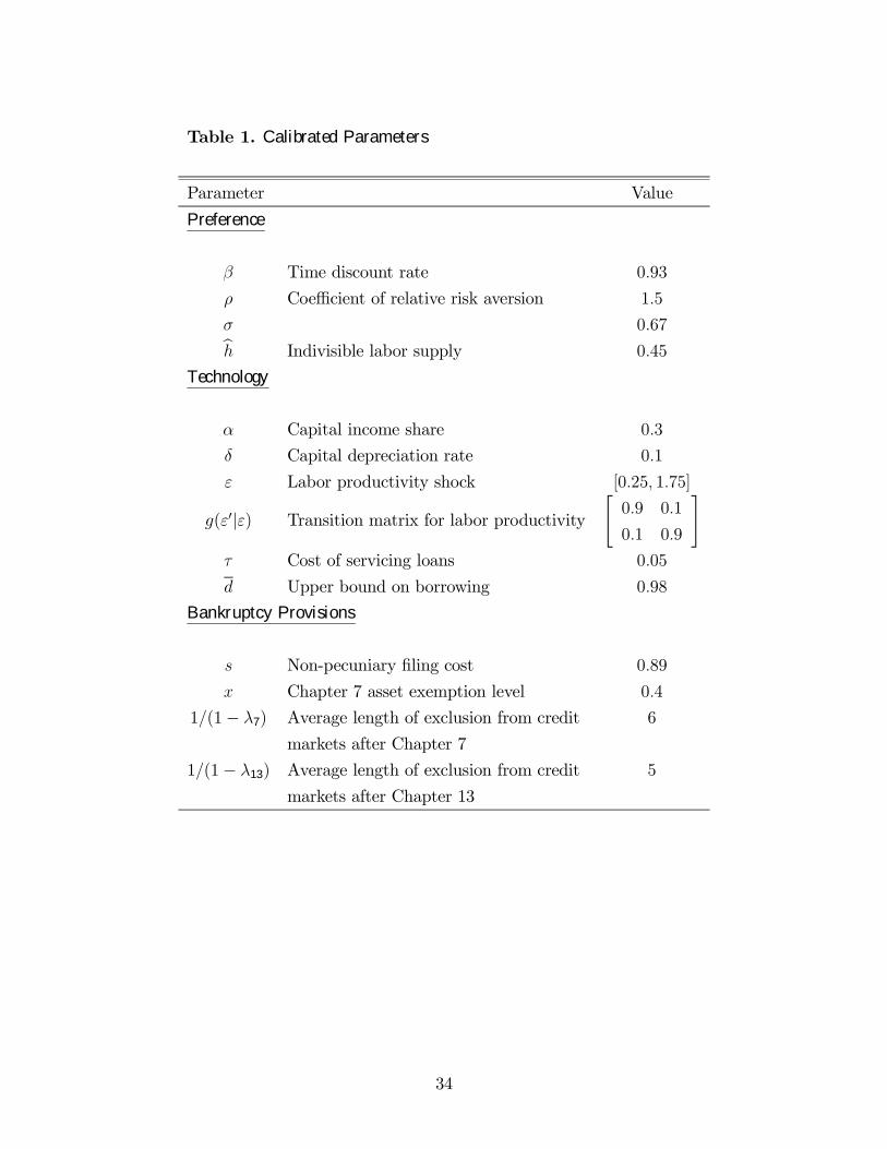
Table 1. Calibrated Parameters
Parameter Value
Preference
� Time discount rate 0�93
Coefficient of relative risk aversion 1�5
' 0�67b� Indivisible labor supply 0�45
Technology
& Capital income share 0�3
� Capital depreciation rate 0�1
� Labor productivity shock [0�25� 1�75]
�(�0|�) Transition matrix for labor productivity
"0�9 0�1
0�1 0�9
#� Cost of servicing loans 0�05
� Upper bound on borrowing 0�98
Bankruptcy Provisions
� Non-pecuniary filing cost 0�89
� Chapter 7 asset exemption level 0�4
1�(1− �7) Average length of exclusion from credit 6
markets after Chapter 7
1�(1− �13) Average length of exclusion from credit 5
markets after Chapter 13
34

Table 2. The Benchmark Model Economy
Statistics U.S. Data Model
Risk premium (%) 10.8 10.5
Capital/output 2.5 2.4
Debt/income 0.09 0.10
Gini index of income 0.44 0.45
Percentage of defaults (%)
Total 1.18 1.25
Chapter 7 0.83 0.86
Chapter 13 0.35 0.39
Table 3. Implementing the Bill: Means-testing for Chapter 7 Filers
Efficient Driving Out
Statistics Benchmark Means Testing Chapter 7 Defaults
() ≤ 0�37) () ≥ 0�40)(% change from benchmark)
Deposit rate (%)(1) 2.516 2.516 +0.011
Lending rate (%) 13.008 13.008 −0.175Debt/income 0.104 0.104 +4.047
Savings 1.412 1.412 +0.008
Capital 1.366 1.366 −0.264Labor 0.392 0.392 −0.114Output 0.570 0.570 −0.171Welfare −0.761 −0.761 −1.010Chapter 7 filings (%) 0.860 0.860 −0.860Chapter 13 filings (%) 0.386 0.386 +0.708
Total filings 1.246 1.246 −0.151Wealth Gini 0.484 0.484 +0.207
Note 1. For the deposit rate, as well as all variables already expressed in percent,
changes from the benchmark are in levels.
35

Table 4. Alternative Policy Changes
Tightening asset exemptions
Benchmark under Chapter 7 Eliminating bankruptcy
Statistics (� = 0�4) (� = 0�375)(2) provisions entirely
(% change from benchmark) (% change from benchmark)
Deposit rate (%) 2.516 −0.023 +0.596
Lending rate (%) 13.008 +0.027 −4.867Debt/income 0.104 −6.013 +34.146
Savings
Total 1.412 −0.046 +1.873
Ave. Chap. 7 filer 0.003 −33.33 N/A
Ave. Chap. 13 filer 0.160 −0.125 N/A
Consumer debt
Ave. Chap. 7 filer 0.167 +0.119 N/A
Ave. Chap. 13 filer 0.196 −0.101 N/A
Capital 1.366 +0.326 −8.989Labor 0.392 +0.053 −2.430Output 0.570 +0.133 −4.447Welfare −0.761 +0.421 −3.330Chap. 7 filings (%) 0.860 +0.109 N/A
Chap. 13 filings (%) 0.386 −0.375 N/A
Total filings (%) 1.246 −0.265 N/A
Gini (wealth) 0.484 −0.206 +1.240
Note 2. The case � = 0�375 maximizes steady state welfare.
36

a (assets)x/R a* a**
Vchap. 7(a,ε)
V (value function)
Vchap. 13(a,d',ε)
Vchap. 13(a,d,ε)
d increases to d' > d
Figure 1. The Effects of Assets and Debt on Bankruptcy Choice
37

38