The marginal propensity to hire∗

Davide Melcangi

University College London†

December 2017

Job Market PaperPlease click here for the most recent version

Abstract

This paper studies the link between firm-level financial constraints and employment decisions, as

well as the implications for the propagation of aggregate shocks. I exploit the idea that, when the

financial constraint binds, a firm adjusts its employment in response to cash flow shocks. I identify

such shocks from changes to business rates, a UK tax based on a periodically estimated value

of the property occupied by the firm. A 2010 revaluation implied that similar firms, occupying

similar properties in narrowly defined geographical locations, experienced different tax changes,

allowing me to control for confounding shocks to local demand. I find that, on average, for every

£1 of additional cash flow, 39 pence are spent on employment. I label this response the Marginal

Propensity to Hire (MPH). I then calibrate a firm dynamics model with financial frictions towards

this empirical evidence. As in the data, small and leveraged firms in the model have a greater

MPH. Simulating a tightening of credit conditions, I find that the model can account for much of

the decline in UK aggregate output and employment observed in the wake of the financial crisis.

Keywords: financial frictions, employment, heterogeneous firmsJEL classification: E24, E44, G01, G32

∗I am grateful to Vincent Sterk and Marco Bassetto for invaluable advice and guidance, and also toMorten Ravn for insightful suggestions and discussions. For helpful comments, I also thank Wendy Carlin,Wei Cui, Ralph Luetticke, Franck Portier, Javier Turen, Mimosa Distefano, Silvia Sarpietro and Carlo Galli.I thank the UK Data Service for guidance and assistance with regard to the data. Data contains informationprovided by the Valuation Office Agency under the Open Government Licence v3.0. The UK Data Serviceagrees that the outputs are non-disclosive, and cannot be used to identify a person or organisation. The useof the BSD data does not imply the endorsement of the data owner or the UK Data Service at the UK DataArchive in relation to the interpretation or analysis of the data. This work uses research datasets which maynot exactly reproduce National Statistics aggregates.†Department of Economics and Centre for Macroeconomics, address: Drayton House, 30 Gordon Street,

London, WC1H 0AX, United Kingdom. E-mail: d.melcangi.12@ucl.ac.uk

1

1 Introduction

The rise in unemployment following the financial crisis has underscored the importanceof links between financial and labour markets. The long-standing challenge that this lit-erature faces is the identification of financially constrained firms, which remains difficult.This implies it is also difficult to pin down the role that these constraints actually play forfirms’ employment decisions and, in turn, for macroeconomic dynamics.

In this paper, I exploit the idea that, when financial constraints bind, a firm adjusts itsemployment in response to cash flow shocks. I label this response the marginal propensityto hire (MPH). Consider a cash flow shock that is uncorrelated with the firm’s productionfrontier and demand. When unconstrained, the firm is at its optimal size and therefore itsemployment decisions are neutral to the additional cash flow. When constrained, instead,the firm uses the additional cash flow to hire more workers and expand its size: the MPHis positive in this case.

This paper entails two main contributions. First, I use a novel combination of threelarge data sets from the UK and a new source of variation to estimate how employmentresponds to cash flow shocks and how the MPH varies across firms. Second, I use thisempirical evidence as an input to discipline a theoretical model that combines firm hetero-geneity and financial frictions. I use the calibrated model to shed light on the heterogeneityof the MPH that is found in the data and to study the aggregate responses to a tighteningin credit conditions, as well as their relation to the moments of the MPH distribution.

Although cash flows can be measured, it is difficult to come by exogenous variation. Iidentify cash flow shocks from changes to business rates, a UK tax based on a periodicallyestimated value of the property occupied by the firm. The fact that business rates are notexplicitly related to firm performance makes changes to this tax a good candidate forthe identification of such shocks. Estimated rental values used to compute the businessrates are typically re-assessed every five years, and the infrequency of the revaluation maycause sharp changes to the tax liability.1 Focusing on the revaluation which took placein 2010, I document that a high degree of variation in tax bill changes persists even ata narrow geographical level and within similar types of properties. When re-estimatingthe rental values, properties are grouped in valuation schemes by a government agency,which then makes assumptions over the standard property in each scheme; this formsthe basis of the revaluation. The creation of more than 60 thousand schemes, which aredefined geographically at a very narrow local level, introduces a lot of the aforementionedvariation. This allows me to control for relevant confounding factors as local demandshocks. I estimate the MPH by comparing the net hiring of similar firms, occupying

1See, for instance, the IFS 2014 Green Budget and the article “Southwold: welcome to the town wherebusiness rates are set to rise 177%”, published by The Guardian on 9 March 2017.

2

similar properties, in the same geographical area, which face different revaluations.I construct a unique dataset that combines employment data at the establishment and

firm level with balance sheet data at the firm level and tax data at the property level.Employment data is sourced from the Business Structure Database (BSD), a confidentialpanel that comprises the near universe of UK firms - around 2.5 million per year - from1997 to 2016. Balance sheet data between 2006 and 2015, for around 1.5 million firms,are taken from FAME (Financial Analysis Made Easy). Finally, tax bills are calculatedusing information from the Valuation Office Agency (VOA), which covers 1.9 millionbusiness property valuations in England and Wales for 2005 and 2010. My data set hasseveral advantages. First, it allows for the identification of cash flow shocks in a verybroad sample, while addressing relevant endogeneity concerns. Second, it enables meto study the role of financial constraints on employment, which has received much lessattention than the vast literature on investment-cash flow sensitivity arising from Fazzariet al. (1988). Third, the data used in my work mainly consist of small firms, often young,and that are typically not publicly listed. Private firms may rely more heavily on exter-nal finance, as documented by Zetlin-Jones and Shourideh (2017). These features makeFAME and the BSD particularly suitable for the study of financial frictions.

I estimate that, for every additional £1 of cash flow generated by the tax revaluation,on average 39 pence are spent on employment. The richness of the data allows me toaddress relevant endogeneity issues, such as local and idiosyncratic shocks, and anticipa-tion. Firms’ employment does not respond to future cash flow shocks and the results arenot driven by the non-tradable sector, which is typically more sensitive to local demand.By ruling out relocations and physical changes to the property following the revaluation,I exclude the possibility that the employment response is driven by endogenous locationmotives or changes to the cost of capital, rather than by the cash flow channel. The MPHvaries depending on firm characteristics: I find that employment at small and more lever-aged firms is more responsive to cash flow shocks.

I then build a heterogeneous-firm model with financial frictions that is motivated anddisciplined by the empirical evidence on the MPH and its heterogeneity. Firms in themodel are heterogeneous ex-post due to persistent idiosyncratic productivity and face twofinancial frictions. First, they cannot issue equity. Second, they need to pay the wage billin advance of production and face a working capital collateral constraint as in Jermannand Quadrini (2012). The model is rich enough to match a wide range of micro featuresof the data; at the same time, its tractability enables me to derive a closed-form analyti-cal formula for the MPH. When both financial constraints bind, firms are willing to useadditional cash flow to increase their future wealth. This increases their ability to takeup working capital loans and thus allows them to hire more workers, implying a positive

3

MPH. Moreover, constrained firms have a marginal product of labour that is greater thanthe wage, and I find that this gap is positively correlated with the MPH.

The model is calibrated to reproduce both macro- and micro-economic features of thedata, as well as the average MPH estimated in the empirical analysis. I use the modelto uncover the mechanisms behind the MPH. First, the model generates a distribution ofmarginal propensities to hire and endogenously replicates the heterogeneity found in thedata. Small and more leveraged firms are more likely to be credit-constrained and dis-play increasingly greater employment-cash flow sensitivities. Second, I use the model tostudy how each parameter affects the distribution of the MPH by influencing the extensivemargin – i.e.: the share of constrained firms –, the intensive margin – i.e.: the firm-levelendogenous tightness of financial frictions –, or both. While all the model parametersaffect the MPH, I find that the capital endowment of entrants is particularly informative.This parameter can be interpreted as an additional financial friction on start-up loans.

I study the response of the calibrated economy to an unexpected tightening of creditconditions, calibrated to match the fall in net debt in the UK between 2008 and 2011. Themodel can account for much of the decline in aggregate employment and output experi-enced by the UK during the Great Recession. I also investigate how relevant momentsof the MPH distribution can inform policymakers and macroeconomists about the differ-ential responses to aggregate shocks. Analytically, I show that the response of aggregateemployment to a credit tightening depends positively both on the average MPH and on thecovariance between MPH and firm size. Given that the model parameters typically affectthese moments in opposite directions, which effect prevails in the aggregate is a quantita-tive question. Numerically, I find that economies with a greater average MPH, achievedby changing the capital endowment of entrants, display a larger and more prolonged fallin aggregate employment following a credit tightening episode.

The findings of this paper have several policy implications. The sensitivity of employ-ment to cash flow may be informative about the design and the effectiveness of policiessuch as targeted subsidies. For instance, the heterogeneity of the MPH with respect tofirm size can be related to the debate on size-dependent policies.2 Moreover, the modelshows that knowing the average MPH and the covariance between MPH and firm size isimportant in order to assess the sensitivity of aggregate employment to the tightness of thefinancial friction as well as for the effectiveness of stabilisation policies. I find that bothmoments fall during a credit tightening. This implies that uniform transfers may be lesseffective in those periods, given the lower average sensitivity of employment to additionalcash flow, while targeting small firms may boost aggregate employment more.

2See Guner et al. (2008) on the topic. Cahuc et al. (2014) investigate the effectiveness of hiring creditsintroduced in France in 2009, which were targeted to firms with less than 10 employees. In recent years,the UK government has put in place a set of small business grants that depend on firm size.

4

The paper is organised as follows. In Section 2, I describe extensively the businessrates, the revaluation process and document evidence of the extent of the variation in taxchanges. After describing the data in section 3, I present the main reduced-form findings,in the form of average MPH and its robustness to a wide set of confounding factors (sec-tion 4). Sections 4.3 and 4.4 investigate the response to balance sheet variables other thanemployment and the MPH heterogeneity in the data. The model is presented thereafter(section 5), while section 6 describes the calibration and how different parameters affectthe MPH. Finally, section 7 deals with the macroeconomic implications of the MPH.

Related literature

A large body of academic work has studied the sensitivity of investment to cash flow andits relation with financial constraints.3 The long-standing issue faced with this literatureis the identification of cash flow shocks and, in turn, of financially constrained firms.Indeed, cash flow may contain information on future profitability, thus driving a spuriouscorrelation with investment. More recent papers try to identify arguably exogenous shocksto internal funds. Among others, Rauh (2006) exploits defined-benefit pension refundingshocks. My paper proposes a new source of exogenous variation and a large dataset whichallows me to study the response of the whole distribution of firms. This includes private,small and young firms, which are expected to be more affected by financial frictions.

My paper shifts the focus from the impact of financial constraints on capital investmentto their influence on employment decisions. A few papers have recently studied empiri-cally the interaction between financial constraints and employment. Schoefer (2015) esti-mates the dollar-for-dollar sensitivity of employment to cash flow and uses this to motivatea search and matching model with wage rigidity among incumbent workers and financialfrictions. He borrows identification strategies from the investment literature and estimatesemployment - cash flow sensitivities ranging between 0.22 and 0.72. His empirical anal-ysis, however, is limited to publicly listed firms. Chodorow-Reich (2013) investigates theeffect of bank lending frictions on employment outcomes. Compared to their work, I canmeasure the size of the cash flow shock and therefore the employment response to £1 ofadditional cash flow.4 Giroud and Mueller (2017) find that more leveraged firms cut moretheir employment in response to consumer demand shocks in the Great Recession.

My paper also fits into the vast literature that incorporates firm-level financial frictionsin models of firm dynamics. In corporate finance, most of the literature focuses on the role

3See Hubbard (1998) for a survey and Kaplan and Zingales (1997).4Benmelech et al. (2015) also test for the causal effect of financial constraints on firm employment

decisions looking at three quasi experiments: exploiting heterogeneity in the maturity of long-term debt,analyzing the impact of bank deregulation across the United States in the 1970s and exploiting a loan supplyshock originating in Japan in the 1990s.

5

played by financial constraints in distorting investment decisions, as surveyed by Strebu-laev and Whited (2012).5 In particular, labour is typically hired on the spot market andfirms can always implement the static optimum: this implies that financial frictions haveno direct and independent effect on employment decisions.6 By explicitly modelling alink between labour demand and financial frictions, my model contributes to the literatureby formalizing the concept of a marginal propensity to hire out of cash flow shocks andstudying its theoretical and quantitative properties.

Finally, this paper is related to a growing macro literature that focuses on firm-levelfinancial frictions, as surveyed by Quadrini (2011). Among seminal and influential con-tributions, Gertler and Gilchrist (1994) and Bernanke et al. (1999) propose a “financialaccelerator” mechanism that amplifies and propagates shocks to the macroeconomy. Theysuggest that small firms are more affected by financial constraints, a feature corroboratedboth by the empirical and theoretical parts of my paper. As in Jermann and Quadrini(2012), the financial constraint considered in my model shows up as a labour wedge.Moreover, I embed this framework in a heterogeneous firm setting, shedding light on theinteraction between labour and finance in the cross-section. Recent papers have inves-tigated the effect of shocks to financial constraints in a model with firm heterogeneity.Among others, Khan and Thomas (2013) focus on capital misallocation, while Bassettoet al. (2015) on the differential impact on corporate and entrepreneurial sector. Buera etal. (2015) introduce search frictions in a model of producer heterogeneity to argue that acredit crunch can translate onto a protracted increase in unemployment. My paper hintsat the relevance of additional statistics, associated with the marginal propensity to hire, tocorrectly calibrate this type of models and draw macroeconomic implications.

2 Business Rates revaluation

Occupiers of business property in the UK pay each year a tax, the business rates, which isa percentage of the estimated market rental value of the property.7 Occupiers are liable topay the tax regardless whether they own or rent the property. Business rates raised £26.1billion in 2012-13, which was 4.5% of total fiscal revenues and the equivalent of twothirds of the amount raised by corporate tax. Recurrent taxes levied on business property

5An exception is Michaels et al. (2016), who integrate costly external finance with both labor and capitaldemand. Empirically, they document that wages and leverage are strongly negatively correlated; their modelshows that both financing frictions and wage bargaining are important to reproduce this finding.

6A separate strand of literature has recently introduced financial frictions in search models. Boeri et al.(2017) study the interaction between labour and financial frictions and its role for firms’ incentives to holdliquidity.

7Business rates is the common denomination for non-domestic rates. This study uses data for Englandand Wales. Business rates are also levied in Scotland and Northern Ireland, but they are handled differently.

6

in the UK are among the highest in the OECD.8

The tax liability is calculated by multiplying a percentage, called business rates mul-

tiplier, by the rateable value, which is the estimated market rental value of the property.9

Every five years, the Valuation Office Agency (VOA) re-estimates the rateable values forEnglish and Welsh properties, and this revaluation triggers the tax changes studied in thispaper.10 Multipliers are instead updated every year in line with the Retail Price Index(RPI). In revaluation years, the multiplier is adjusted so that the average bills increase inline with RPI inflation. This implies that the impact of revaluations is purely redistribu-tive, creating winners - properties for which the tax liability falls after the revaluation - andlosers - properties that experience an increase in their tax bills. Since business rates are setnationally, the revaluation is not affected by discretionary incentives of the policymaker.

The revaluation that took effect on 1 April 2010 is the object of this study. I documenta large degree of variation in tax changes even at fine local level and among similar prop-erties. Figure 1 shows the average change in the business rates liability due to the revalua-tion, at the postcode sector level for large offices in the Manchester area. Although there issome spatial correlation across postcode sectors, it is not infrequent to observe neighbour-ing areas with very different average tax changes. Tax changes vary significantly even atnarrower geographical level. For each postcode sector in England and Wales, I computethe standard deviation of tax changes for large offices. The average standard deviation is£8,150 (12% in growth terms) and the average range £29,771 (32%).11

What is the source of this large variation? To answer this question, it is useful topresent the 2010 revaluation process in more detail. The VOA collected rent informationfrom business tenants and used this to estimate the rateable values, defined as a reasonablerent as of 1 April 2008, under full repairing and insurance terms. Similar propertiesin an area were grouped together in a valuation scheme; within each scheme, the VOAmade assumptions about the standard property, which formed the basis for the valuationof each property in the scheme. Finally, each rateable value was adjusted to accountfor idiosyncratic differences within the scheme.12 Hence the source of variation is two-fold: it is partly due to the assignment to different valuation schemes, and partly down toproperty-specific differences within each scheme.

The creation of 60,022 valuation schemes introduced many discontinuities and the

8OECD data on receipts from recurrent taxes on immovable property, levied on non-households, as ashare of national income in 2011. Data is not available for a small set of countries as US, Japan and Italy.

9The rateable value broadly represents the annual rent the property could have been let for on the openmarket on the reference date, on full repairing and insuring terms. Hence the rateable value will be typicallydifferent from the rent that is actually be paid on the property.

10The last revaluation was delayed by two years and took place in 2017.11On average there are 10 large offices in a postcode sector (median is 4). The average standard deviation

increases to £12,763, and the range to £64,960, when looking at postcode sectors with at least 10 properties.12For example a property without air conditioning belonging to a scheme which assumes it.

7

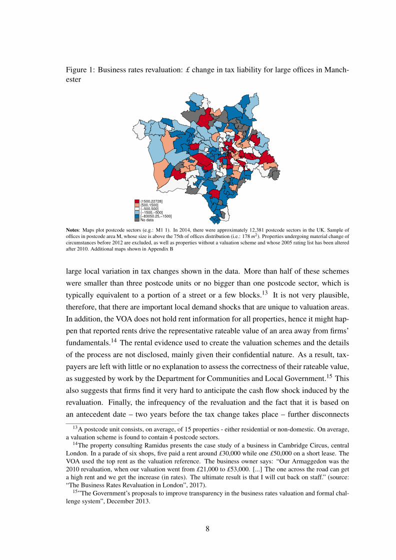
Figure 1: Business rates revaluation: £ change in tax liability for large offices in Manch-ester

(1500,22728](500,1500](−500,500](−1500,−500][−83050.25,−1500]No data

Notes: Maps plot postcode sectors (e.g.: M1 1). In 2014, there were approximately 12,381 postcode sectors in the UK. Sample ofoffices in postcode area M, whose size is above the 75th of offices distribution (i.e.: 178 m2). Properties undergoing material change ofcircumstances before 2012 are excluded, as well as properties without a valuation scheme and whose 2005 rating list has been alteredafter 2010. Additional maps shown in Appendix B

large local variation in tax changes shown in the data. More than half of these schemeswere smaller than three postcode units or no bigger than one postcode sector, which istypically equivalent to a portion of a street or a few blocks.13 It is not very plausible,therefore, that there are important local demand shocks that are unique to valuation areas.In addition, the VOA does not hold rent information for all properties, hence it might hap-pen that reported rents drive the representative rateable value of an area away from firms’fundamentals.14 The rental evidence used to create the valuation schemes and the detailsof the process are not disclosed, mainly given their confidential nature. As a result, tax-payers are left with little or no explanation to assess the correctness of their rateable value,as suggested by work by the Department for Communities and Local Government.15 Thisalso suggests that firms find it very hard to anticipate the cash flow shock induced by therevaluation. Finally, the infrequency of the revaluation and the fact that it is based onan antecedent date – two years before the tax change takes place – further disconnects

13A postcode unit consists, on average, of 15 properties - either residential or non-domestic. On average,a valuation scheme is found to contain 4 postcode sectors.

14The property consulting Ramidus presents the case study of a business in Cambridge Circus, centralLondon. In a parade of six shops, five paid a rent around £30,000 while one £50,000 on a short lease. TheVOA used the top rent as the valuation reference. The business owner says: “Our Armaggedon was the2010 revaluation, when our valuation went from £21,000 to £53,000. [...] The one across the road can geta high rent and we get the increase (in rates). The ultimate result is that I will cut back on staff.” (source:“The Business Rates Revaluation in London”, 2017).

15”The Government’s proposals to improve transparency in the business rates valuation and formal chal-lenge system”, December 2013.

8

rateable values from current firms’ fundamentals.16

The features of the revaluation and the fact that similar properties in the same geo-graphical area experienced different tax changes make the latter a good candidate for theidentification of plausibly exogenous cash flow shocks. Most importantly, this relies onthe fact that business rates “bear little or no relation to (firms’) turnover, profits or abilityto pay. Instead, it is arbitrarily based upon notional property values.”17 Section 4 discussesthe identification assumptions in detail.

3 Data

I construct a unique dataset that combines employment data at the establishment and firmlevel with business rates tax data at the property level and balance sheet data at the firmlevel. The employment data are provided by the Office for National Statistics (ONS)Business Structure Database (BSD). This dataset contains a small number of variables foralmost all business organisations in the UK. It consists of a series of annual snapshots,taken around April, of the Inter-Departmental Business Register (IDBR). The IDBR isa live register of data collected via administrative records. I combine them in a longi-tudinal panel of establishments and firms for the years 1997-2016. The tax data comesfrom the Valuation Office Agency and contains nearly all - 1.9 million - business propertyvaluations in England and Wales for the 2005 and 2010 rating lists, linked by a propertyidentifier.18 It contains details of the location and rateable values of each property, as wellas property characteristics and the valuation scheme numbers as contained in the Sum-mary Valuation (SMV) files. Balance sheet and income statement data are taken fromFAME (Financial Analysis Made Easy), as provided by the Bureau van Dijk. I considera panel of roughly 1.2 million UK firms, for the years 2006 - 2014, which can be mergedwith the BSD data. This is a much broader sample than other alternatives often used inliterature, as it is not limited to publicly listed firms, as US Compustat, but it mainly con-tains private limited companies (96% of the sample). Indeed, the UK Companies Houserequires all incorporated companies to disclose balance sheet information. Appendix A.1provides extensive information on each data source and the details of the dataset creation.

The main bulk of the analysis uses information on the first two datasets. Tax data at theproperty level is matched with BSD establishment data; given the confidential nature of

16Dentons, the world’s largest law firm, commented that commercial property rents fluctuate constantlywhile business rates are slow to respond, “creating unrealistic rateable values” (source: “Rating – the roadto revaluation: Reform”, Lexology, March 30 2017).

17Source: ”Business Rates - an Unfair System”, 16 February 2017, Federation of Small Businesses.18This allows me to construct only one tax change. Extending the dataset over time, thus incorporating

information on revaluations at different years, would help significantly the identification of the MPH and itsheterogeneity, besides the features of the MPH distribution.

9

the BSD data, business rates unique addresses cannot be used. Hence, I merge the datasetsusing postcode unit information and create a mapping between establishment-level indus-try codes and property type. In the UK, a postcode unit is typically very small, generallyrepresenting a street, part of a street or even a single property. There are approximately1.75 million postcodes in the United Kingdom according to the ONS. I keep the establish-ments that remain active between 2009 and 2011 and do not change location. I am ableto match 174,726 establishments with the properties they occupy; this is associated with135,139 firms. This matching strategy allows me to evaluate firms’ responses to a change

in the tax liability they actually face. On the other hand, it leaves out the establishmentsthat cannot be uniquely matched to their properties. For instance, if in the same postcodeunit there is more than one shop and more than one establishment in the retail or whole-sale sector. Appendix A.4 shows that the estimated coefficients are qualitatively similar tothe benchmark estimates when averaging over postcodes-industry-property type groups.

Appendix A.1 describes the sampling strategy in detail.19 I exclude the propertiesincurring in physical changes after the revaluation and before 2012. Indeed, firms havethe possibility to reduce their tax bill by changing the features of the property and thenreporting a material change of circumstances to the Valuation Office Agency.20 This mayimply a change in employment due to the complementarity with fixed assets and followinga response to a change in the user cost of capital; since, instead, I am interested in thebalance sheet channel of cash flow shocks, I exclude this possibility. Finally, I drop theconstruction sector, because of its specific nature when it comes to a property tax. Afterthese sample selections, the dataset contains 82,506 establishment-tax observations.

4 Empirical strategy

The empirical strategy aims at estimating the effect of cash flow shocks induced by thebusiness rates revaluation on firms’ employment decisions. I consider the followingbenchmark specification for a firm i, in the industry sector k occupying a property j inthe geographical area m:

∆2009,11Ei,k, j,m = α +β∆2009,10Tj + γxi,2008 +θz j,2008 +µk,2008 +Pm + εi,k, j,m (1)

19Excluded observations include public sector establishments, properties without a valuation schemereference number and establishments that changed enterprise between 2009 and 2011.

20Material change of circumstances typically involve matters affecting the physical state or physicalenjoyment of the hereditament and the category of occupation of hereditament (Rating Manual Volume 2Section 5). While potentially still working through the balance sheet, the cash flow shock may depend onthe marginal product of capital and driven by other reasons such as endogenous location choices.

10

where the outcome variable ∆2009,11Ei,k, j,m is the change in employment at the firm i

between 2009 and 2011 and ∆2009,10Tj is the £ change in the tax liability at the propertyj, induced by the business rates revaluation in 2010. Firms may have multiple estab-lishments and thus occupy multiple properties. In order to directly exploit property andgeographic characteristics used for identification, for each firm i I retain the property j

associated with the largest (in absolute value) tax change. In appendix A.3 I show that theresults are robust to different specifications for multiple-establishment firms, also because86% of firms in the sample have only one establishment. x, z, µ and P are sets of firm,property, industry and geographical controls, respectively, which are discussed below.21

I identify the effects of cash flow shocks on employment changes by comparing sim-ilar firms, occupying similar properties in the same geographical area. The coefficient ofinterest is β . Correct identification hinges on the fact that there is neither omitted vari-able simultaneously affecting the business rates and employment, nor reverse causality.There are three main possible confounding factors that may affect identification. First,there could be local shocks that simultaneously affect employment and the business rates.Second, shocks idiosyncratic to the firm may affect employment and - via physical im-provements - the estimated rateable value of the property. Finally, cash flow changesinduced by the revaluation may be anticipated. I now discuss how different controls areaimed at addressing these issues.

The inclusion of postcode area dummies Pm for the location of the property is moti-vated by the attempt to control for local shocks and anticipation. Being based on rentalevidence, tax changes vary across geographical areas. I decide to consider geographicalunits for which it is reasonable to think that a firm may be aware of the trends in rents andanticipate at least part of the tax change. The benchmark specification considers postcodearea dummies. A postcode area is formed by the initial characters of the alphanumericUK postcode. For instance, the postcode area N stands for North London. In 2014 therewere 124 postcode areas in the UK (source: ONS). Standard errors are clustered at thislevel. I also consider tighter specifications at the postcode district level.22

Industry-specific shocks may simultaneously affect tax changes and employment. Whilebusiness rates in levels could be correlated with firm industry through real estate inten-sity, it is less clear ex ante how business rates revaluations could reflect industry-specificshocks. A certain industry may have, for instance, experienced a boom which boostedemployment and the rents of properties typically used in that industry, thus in turn imply-

21All controls are measured before the tax change takes place. Property features may be different beforeand after the revaluation; moreover, firms may change industry. Section 4.2 looks specifically at these cases.

22A postcode district typically identifies a town and the surrounding villages (e.g.: BA6 for the area ofGlastonbury), most part of a bigger city (e.g.: GL1 for the centre of Gloucester, a city with a population ofaround 130,000 people) or part of a local authority/borough in London (e.g.: N3 for Barnet). In 2014 therewere 3,114 postcode districts in the UK according to the ONS.

11

ing a tax increase upon revaluation. As in most of the endogeneity issues of this paper,we expect that, if present, this channel should bias the MPH downwards. To clean out thispossible channel, I control for firm-level industry dummies µk,2008 defined at the sectionlevel of UK SIC 2007 codes.23

Finally, I introduce firm controls measured in 2008 and property controls before therevaluation. Property controls consist of property type, the tax bill in 2008 and the prop-erty size measured in square meters. I define three dummies for the property type: whethera property is an office, a shop or a factory/warehouse.24 These dummies play a similar roleto industry dummies. Moreover, they control for the possibility that firms partly antici-pate the tax change by having information on rent trends for specific types of properties.I complement these dummies with a set of industry dummies before the revaluation at theestablishment level.25 The size of the property and the tax bill may correlate with the sizeof the tax change. Since identification exploits both the sign and the size of the tax change,it seems sensible to control for these features. The same applies to firm pre-determinedcharacteristics, namely the inverse of average sales of firm i in 2007 and 2008 and thenumber of firm employees in 2008. Moreover, controlling for firm size helps addressingthe concern that the ability to predict the tax change may correlate with firm characteris-tics, with different anticipation effects and a possible threat to correct identification.

4.1 The average MPH

Table 1 shows the employment effects of the changes in the business rates liability in-duced by the 2010 revaluation. The explanatory variable of interest, ∆2009,10Tj,m, is thedifference in tax bill to be paid at the property j before and after the revaluation. The taxbill is obtained by multiplying the multiplier (tax rate) for the specific year by the rateablevalue estimated by the VOA in that year. After the 2010 revaluation, a transitional reliefwas introduced in England, aimed at phasing in sharp changes in the tax bills. Tax shockscalculated here are before any relief: appendix A.2 deals extensively with this. The taxchange is scaled by firm i average sales in 2007 and 2008, to improve comparability acrossfirms.26 The dependent variable shown in the first 5 columns is the level change in em-

23Examples of section levels are manufacturing, education, information and communication. There are18 sector sections in the sample.

24I construct these dummies by pooling together similar categories, which are by far the most recurrentand represent almost half of the sample. Sometimes a valuation scheme pools different property typestogether; hence adding these dummies may be ”controlling away” some of the effects I am trying to estimate.In unreported results, I show that the estimation results are robust to a broader definition of shops, such that60% of the properties in the sample are assigned to one of the three property types. Similarly, the MPHcoefficient is slightly lower but still significant at 1% if we control for all categories as defined by the VOA.

25These may differ from firm-level industry dummies only for firms with multiple establishments. Theirinclusion leaves the MPH coefficient basically unchanged.

26Results are robust to rescaling by either year.

12

Table 1: The average MPH

∆2009,11Emp ∆2009,11Log(Emp)

(I) (II) (III) (IV) (V) (VI) (VII) (VIII)

∆2009,10T −0.34∗∗∗ −0.40∗∗∗ −0.39∗∗∗ −0.36∗∗∗ −0.41∗∗∗ −0.59∗∗∗ −0.72∗∗∗ −0.72∗∗∗

(0.10) (0.11) (0.11) (0.11) (0.16) (0.17) (0.17) (0.18)

Postcode area FE X X X X X XIndustry dummies X X X XFirm controls X X X XProperty controls X X X XPostcode area x industry FE XPostcode district x industry FE X

Observations 63,242 63,242 63,242 63,242 63,242 63,242 63,242 63,242R2 0.00 0.01 0.01 0.02 0.03 0.00 0.01 0.01

Note: ∆2009,11Emp is the change in the number of employees at firm i, rescaled as explained in the text. ∆2009,10T is the scaledtax change as explained in the text. Industry dummies are measured in 2008, at the firm-level, and defined at the section level ofUK SIC 2007 codes. Firm controls include firm i number of employees in 2008 and the inverse of average sales between 2007 and2008. Given the timing of the data, it should be noted that I define firm sales in 2008 as the value reported in the business register inApril 2008, hence typically referring to the financial year 2007-2008. Property controls consist of the size of the property measuredin m2, the business rates liability in 2008, industry dummies at the establishment level and dummies for whether the property is afactory/warehouse, a shop or an office. Interacting industry dummies at the establishment-level, instead of firm-level, in column IVand V delivers the same results. Standard errors (in parentheses) are clustered at the postcode area level, except for column V in whichthey are clustered at the postcode district level. ∗, ∗∗ and ∗∗∗ denote significance at the 10%, 5% and 1% level, respectively.

ployment at the firm i between 2009 and 2011. I multiply this by a single, constant wage,and divide it by firm i average sales in 2007 and 2008. This rescaling allows me to expressthe MPH coefficient β as the negative of the pound-for-pound sensitivity of employmentto the cash flow changes induced by business revaluation in 2010. For the rescaling, Iuse the median gross annual earning of all employees in 2010, as recorded by the AnnualSurvey of Hours and Earnings;27 this amounts to £21,024. The 2009-2011 horizon foremployment changes is chosen due to the timeline of the revaluation. Draft revaluationswere made public on 30 September 2009, while becoming effective on the 1st April 2010.BSD employment data is a snapshot of the business register as at April each year.

The estimated MPH is fairly insensitive to the inclusion of different sets of controls.Column III suggests that, for every £1 of additional cash flow, 39 pence are spent onemployment. This sensitivity increases slightly as we control for a narrower geographicalarea, the postcode district, interacted with the industry dummies. This tighter specificationcontrols for local shocks specific to an industry in a narrow geographical area, whichmight have simultaneously affected firms’ employment and the estimated rateable values.

Columns VI-VIII show instead the semi-elasticity of employment to the tax shocks. In

27See Appendix A.1 for more details. While being convenient in terms of interpretation, a single wagemasks a good deal of heterogeneity, which may affect the MPH. For instance, the fact that small firms typi-cally pay lower wages and employ more part-time employees (ASHE 2016) may lead to the overestimationof the MPH. For this reason, the estimated coefficient should be referred to employment changes only, andthe wage transformation only as a way to express those changes in £ terms.

13

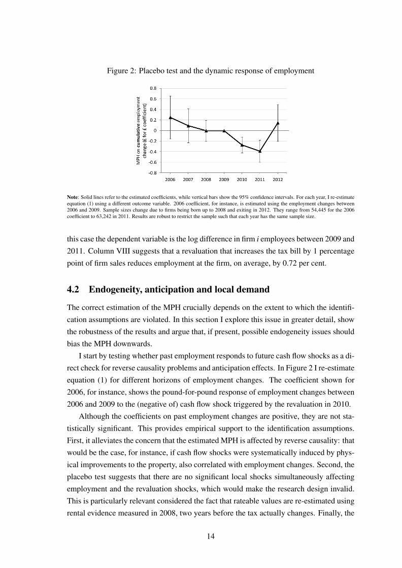
Figure 2: Placebo test and the dynamic response of employment

Note: Solid lines refer to the estimated coefficients, while vertical bars show the 95% confidence intervals. For each year, I re-estimateequation (1) using a different outcome variable. 2006 coefficient, for instance, is estimated using the employment changes between2006 and 2009. Sample sizes change due to firms being born up to 2008 and exiting in 2012. They range from 54,445 for the 2006coefficient to 63,242 in 2011. Results are robust to restrict the sample such that each year has the same sample size.

this case the dependent variable is the log difference in firm i employees between 2009 and2011. Column VIII suggests that a revaluation that increases the tax bill by 1 percentagepoint of firm sales reduces employment at the firm, on average, by 0.72 per cent.

4.2 Endogeneity, anticipation and local demand

The correct estimation of the MPH crucially depends on the extent to which the identifi-cation assumptions are violated. In this section I explore this issue in greater detail, showthe robustness of the results and argue that, if present, possible endogeneity issues shouldbias the MPH downwards.

I start by testing whether past employment responds to future cash flow shocks as a di-rect check for reverse causality problems and anticipation effects. In Figure 2 I re-estimateequation (1) for different horizons of employment changes. The coefficient shown for2006, for instance, shows the pound-for-pound response of employment changes between2006 and 2009 to the (negative of) cash flow shock triggered by the revaluation in 2010.

Although the coefficients on past employment changes are positive, they are not sta-tistically significant. This provides empirical support to the identification assumptions.First, it alleviates the concern that the estimated MPH is affected by reverse causality: thatwould be the case, for instance, if cash flow shocks were systematically induced by phys-ical improvements to the property, also correlated with employment changes. Second, theplacebo test suggests that there are no significant local shocks simultaneously affectingemployment and the revaluation shocks, which would make the research design invalid.This is particularly relevant considered the fact that rateable values are re-estimated usingrental evidence measured in 2008, two years before the tax actually changes. Finally, the

14

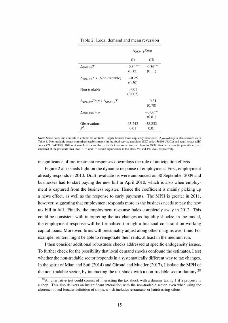
Table 2: Local demand and mean reversion

∆2009,11Emp

(I) (II)

∆2009,10T −0.34∗∗∗ −0.36∗∗∗

(0.12) (0.11)

∆2009,10T x (Non-tradable) −0.25(0.30)

Non-tradable 0.001(0.002)

∆2007,09Emp x ∆2009,10T −0.31(0.78)

∆2007,09Emp −0.06∗∗∗

(0.01)

Observations 63,242 58,252R2 0.01 0.01

Note: Same notes and controls of column III of Table 1 apply besides those explicitly mentioned. ∆2007,09Emp is also rescaled as inTable 1. Non-tradable sector comprises establishments in the food service activities (SIC codes 56101-56302) and retail sector (SICcodes 47110-47990). Different sample sizes are due to the fact that some firms are born in 2008. Standard errors (in parentheses) areclustered at the postcode area level. ∗, ∗∗ and ∗∗∗ denote significance at the 10%, 5% and 1% level, respectively.

insignificance of pre-treatment responses downplays the role of anticipation effects.Figure 2 also sheds light on the dynamic response of employment. First, employment

already responds in 2010. Draft revaluations were announced on 30 September 2009 andbusinesses had to start paying the new bill in April 2010, which is also when employ-ment is captured from the business register. Hence the coefficient is mainly picking upa news effect, as well as the response to early payments. The MPH is greater in 2011,however, suggesting that employment responds more as the business needs to pay the newtax bill in full. Finally, the employment response fades completely away in 2012. Thiscould be consistent with interpreting the tax changes as liquidity shocks: in the model,the employment response will be formalised through a financial constraint on workingcapital loans. Moreover, firms will presumably adjust along other margins over time. Forexample, renters might be able to renegotiate their rents, at least in the medium run.

I then consider additional robustness checks addressed at specific endogeneity issues.To further check for the possibility that local demand shocks confound the estimates, I testwhether the non-tradable sector responds in a systematically different way to tax changes.In the spirit of Mian and Sufi (2014) and Giroud and Mueller (2017), I isolate the MPH ofthe non-tradable sector, by interacting the tax shock with a non-tradable sector dummy.28

28An alternative test could consist of interacting the tax shock with a dummy taking 1 if a property isa shop. This also delivers an insignificant interaction with the non-tradable sector, even when using theaforementioned broader definition of shops, which includes restaurants or hairdressing salons.

15

Table 3: Idiosyncratic shocks

∆2009,11Emp

(I) (II)

∆2009,10T −0.40∗∗∗ −0.39∗∗∗

(0.12) (0.11)

Industry change dummy -0.008∗∗

(0.003)

Property type change dummy -0.005(0.004)

Increase in m2 dummy 0.001(0.002)

Property size unchanged X

Observations 53,444 63,242R2 0.01 0.01

Note: Same notes and controls of column III of Table 1 apply besides those explicitly mentioned. Standard errors (in parentheses) areclustered at the postcode area level. ∗, ∗∗ and ∗∗∗ denote significance at the 10%, 5% and 1% level, respectively.

If business rates revaluations were proxying local demand shocks, we would expect thenon-tradable sector to respond less to tax changes because of higher sensitivity to localdemand. In contrast, the non-tradable sector displays an even greater MPH, although notsignificant, as shown in Column I of Table 2. There may clearly be other reasons behindthis finding; for instance, firms in the non-tradable sector may have, on average, a differentbalance sheet structure.

Revaluations are based on rental evidence in 2008, hence two years before the taxactually changes. In the event of systematic mean reversion, the coefficients may bebiased by endogeneity with respect to past employment growth. Consider a small area thatis doing well in 2008: employment growth would be positive and revaluations may bringalong an increase in the tax liability. If employment growth mean reverts in 2010, whenthe revaluation takes place, the MPH coefficient may be spuriously measuring this meanreversion. In the spirit of Giroud and Mueller (2017), in column II I explicitly control for2007-09 employment growth, as well as its interaction with the tax shock. Although thereare signs of mean reversion, the average MPH remains roughly unchanged.

Finally, I specifically address the possibility that idiosyncratic shocks may affect firmemployment and - via physical improvements - the estimated rateable value and, in turn,the tax change. Column I of Table 3 restricts the sample to the cases in which the size ofa property, measured in square meters, is the same before and after the revaluation. Theestimated MPH is unchanged, further limiting the concerns about idiosyncratic shocksand anticipation. In column II, I explicitly control for property-specific changes around

16

the revaluation. In particular, I augment specification (1) by including three additionalcontrols: a dummy that takes 1 if the firm changed industry between 2008 and 2010,another dummy taking 1 for changes to the property type before and after the revaluationand a third dummy taking 1 when the post-revaluation property size is larger than before.None of these events affects the employment response to the cash flow shock.

The data allow me to control for observable property characteristics. Although unob-servable features, like quality, may drive part of the tax change, it is unlikely that this cansystematically bias the relationship between employment and tax changes.29

4.3 Balance sheet responses

I now examine how firms’ balance sheets and other key variables are affected by cash flowshocks induced by the business rates revaluations. I match the BSD-VOA sample used inthe previous section with the FAME dataset. Since balance sheet reporting requirementsdepend on the legal status of the firm and its features, I am able to match roughly half ofthe sample. Appendix A.7 describes the FAME dataset in detail.

Balance sheet data can be used to estimate the response of firm variables other thanemployment to cash flow shocks, which are shown in Table 4. Column I shows the pound-for-pound sensitivity of employment to tax shocks, as estimated previously, for the re-stricted balance sheet sample. The coefficient is of similar magnitude and significance.

I then estimate equation (1) for different outcome variables related to the balance sheetof the firms. The response of investment to cash flow shocks has been the object of a veryextensive literature, since the seminal contributions of Fazzari et al. (1988) and Kaplan andZingales (1997). Different reporting requirements imply that the granularity of balancesheet data is a function of firm characteristics; for this reason, I define investment as thedifference in fixed assets plus depreciation, when the latter is reported. To be in line withearlier analysis for employment, the time frame is 2009-11.30

The estimated coefficient suggests that business rates revaluations that increase thefirm tax liability imply a reduction in capital investment, although insignificantly differ-ent from zero. To be more in line with the existing literature on investment - cash flowsensitivity, column III uses as a dependent variable capital investment between 2009 and

29A business occupying a property without air conditioning, for example, may anticipate to be includedin a valuation scheme that assumes air conditioning for the representative property. This seems to be beyondthe firm capabilities, however, especially given the absence of underlying rental information. In the sameway, it is hard to think about a mechanism by which a business adds air conditioning to its property, thistranslates into an increase in the tax bill, and then reverberates into a negative change in employment througha channel different than the tax change.

30Appendix A.7 shows robustness to different definitions of investment. The reporting month for thebalance sheet data ranges from July to end of year; results do not change qualitatively when looking atchanges between 2008 and 2011.

17

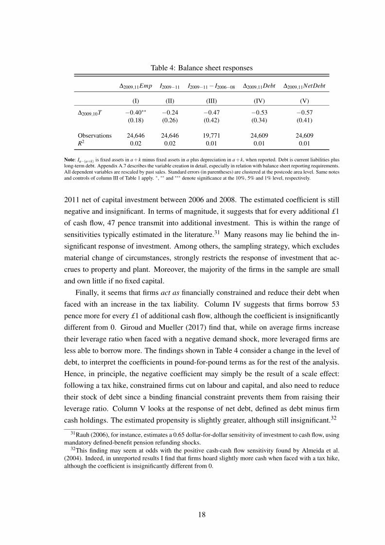
Table 4: Balance sheet responses

∆2009,11Emp I2009−11 I2009−11− I2006−08 ∆2009,11Debt ∆2009,11NetDebt

(I) (II) (III) (IV) (V)

∆2009,10T −0.40∗∗ −0.24 −0.47 −0.53 −0.57(0.18) (0.26) (0.42) (0.34) (0.41)

Observations 24,646 24,646 19,771 24,609 24,609R2 0.02 0.02 0.01 0.01 0.01

Note: Ia−(a+k) is fixed assets in a+ k minus fixed assets in a plus depreciation in a+ k, when reported. Debt is current liabilities pluslong-term debt. Appendix A.7 describes the variable creation in detail, especially in relation with balance sheet reporting requirements.All dependent variables are rescaled by past sales. Standard errors (in parentheses) are clustered at the postcode area level. Same notesand controls of column III of Table 1 apply. ∗, ∗∗ and ∗∗∗ denote significance at the 10%, 5% and 1% level, respectively.

2011 net of capital investment between 2006 and 2008. The estimated coefficient is stillnegative and insignificant. In terms of magnitude, it suggests that for every additional £1of cash flow, 47 pence transmit into additional investment. This is within the range ofsensitivities typically estimated in the literature.31 Many reasons may lie behind the in-significant response of investment. Among others, the sampling strategy, which excludesmaterial change of circumstances, strongly restricts the response of investment that ac-crues to property and plant. Moreover, the majority of the firms in the sample are smalland own little if no fixed capital.

Finally, it seems that firms act as financially constrained and reduce their debt whenfaced with an increase in the tax liability. Column IV suggests that firms borrow 53pence more for every £1 of additional cash flow, although the coefficient is insignificantlydifferent from 0. Giroud and Mueller (2017) find that, while on average firms increasetheir leverage ratio when faced with a negative demand shock, more leveraged firms areless able to borrow more. The findings shown in Table 4 consider a change in the level ofdebt, to interpret the coefficients in pound-for-pound terms as for the rest of the analysis.Hence, in principle, the negative coefficient may simply be the result of a scale effect:following a tax hike, constrained firms cut on labour and capital, and also need to reducetheir stock of debt since a binding financial constraint prevents them from raising theirleverage ratio. Column V looks at the response of net debt, defined as debt minus firmcash holdings. The estimated propensity is slightly greater, although still insignificant.32

31Rauh (2006), for instance, estimates a 0.65 dollar-for-dollar sensitivity of investment to cash flow, usingmandatory defined-benefit pension refunding shocks.

32This finding may seem at odds with the positive cash-cash flow sensitivity found by Almeida et al.(2004). Indeed, in unreported results I find that firms hoard slightly more cash when faced with a tax hike,although the coefficient is insignificantly different from 0.

18

Table 5: MPH heterogeneity in the data

∆2009,11Emp

A = Size A = AgeA = Labourproductivity A = Leverage ratio A = Net leverage ratio

Samples: Whole Whole Whole FAME FAME

(I) (II) (III) (IV) (V)

∆2009,10T x (A≤ A) −0.42∗∗∗ −0.40∗∗ −0.38∗∗ −0.32 −0.16(0.11) (0.16) (0.14) (0.26) (0.23)

∆2009,10T x (A > A) 1.24 −0.38∗∗ −0.52∗∗∗ −0.46∗∗ −0.64∗∗

(0.82) (0.14) (0.14) (0.26) (0.25)

(A≤ A) −0.001 −0.001 −0.02∗∗∗ 0.002 0.003(0.002) (0.002) (0.01) (0.002) (0.002)

Observations 63,242 63,242 63,242 24,633 24,633R2 0.01 0.01 0.01 0.02 0.02

Note: Standard errors (in parentheses) are clustered at the postcode area level. Same notes and controls of column III of Table 1 apply.∗, ∗∗ and ∗∗∗ denote significance at the 10%, 5% and 1% level, respectively. Size is the number of firm i employees in 2008; the cutoffA is 25 employees. Small firms are 87% of the whole sample. Age is the firm age in 2008. The cutoff is 5 years of age; 26% of firmsare classified as young in the whole sample. Labour productivity is the ratio between firm sales in 2008 and the number of employeesat the firm in 2008. The cutoff is the median in the whole sample, which is roughly £66,000 per employee. Median values have beenrounded to the nearest hundred to avoid disclosure issues. Leverage ratio is the ratio of total debt (current liabilities and long-term debt)over total assets. I consider the firm average leverage ratio between 2007 and 2008. The cutoff is the median, 0.60. Net leverage ratiois the ratio of total debt (current liabilities and long-term debt) net of cash over total assets. I consider the firm average net leverageratio between 2007 and 2008. The cutoff is the median, 0.395.

4.4 MPH heterogeneity

How does the MPH vary across firms? The model in section 5 will formalise the linkbetween MPH and financial constraints, and its resulting heterogeneity by firm charac-teristics. The richness of the data, however, also allows me to test whether firm featuresassociated with financial constraints in the literature are associated with stronger employ-ment sensitivity. Table 5 decomposes the coefficients by a set of proxies.

Small firms appear to be the main determinant of the estimated MPH. In column Ifirms have been grouped according to their number of employees in 2008, defining smallfirms as those with less than 25 employees. When interacting the tax shock by a firmage dummy, the difference is less stark; young firms (5 years of age or less) display thesame MPH as old firms. Employment at productive firms, classified as those whose sales-employment ratio in 2008 was above median, responds more to tax shocks.

Finally, more leveraged firms display a greater MPH on average. Column IV classifiesas leveraged the firms whose total debt to total assets ratio before the tax revaluation wasabove the cross-sectional median of the sample. In column V I show that if we net leverageratio with cash holdings, the difference in MPH among groups is even more pronounced.

19

This finding suggests the importance of firms’ liquid assets in assessing the link betweenfinancial constraints and employment. In previous work, I show that cash-intensive firmscut their workforces by less during the Great Recession.

The ex-ante classification of firms by financial constraint proxies has been the objectof controversy in the literature.33 The findings shown in table 5 suggest that small firmsare more affected by financial frictions. Gertler and Gilchrist (1994) proposed size as aproxy for financial constraints, motivated by the fact that small firms exhibit a higher de-gree of idiosyncratic risk and are more bank-dependent. Since then, the literature has de-bated over the differential tightness of financial constraints by firm size, and the resultingsensitivity of small and large firms over the business cycle. Recent work on this includeMehrotra and Crouzet (2017). The MPH heterogeneity also suggests that balance sheetpositions may be related to the endogenous tightness of financial constraints. My findingsecho Giroud and Mueller (2017), who find that more leveraged firms displayed a greatersensitivity to consumer demand in the Great Recession. The structural model presentedin the next section formally links the MPH with financial constraints and endogenouslyreproduces the heterogeneity observed in the data.

5 The model

The empirical findings presented in the previous sections motivate a model of firm dynam-ics in which financial constraints affect hiring decisions directly. In this section I proposea model that combines a working capital collateral constraint, as in Jermann and Quadrini(2012), with firm heterogeneity. The model is tractable enough to derive an analyticalform for the MPH; at the same time, it generates rich cross-sectional dynamics that areconsistent with the empirical findings.

5.1 The firm problem

The economy is populated by a large number of firms, each using pre-determined capitalstock k and labour n to produce a final good. Each firm operates a decreasing returns toscale production function and produces output y according to:

yt = z j,tkνt nα

t , ν +α < 1 (2)

where z j,t is a stochastic and persistent idiosyncratic productivity that follows a Markovchain: z ∈ Z ≡ z1, ..,zNz , with Pr(zt+1 = zi|zt = z j) = π

zji ≥ 0 and ∑

Nzi=1 π

zji = 1. Capital kt

is chosen at time t− 1 while labor nt can be flexibly changed at time t. Capital evolves

33See, for instance, Farre-Mensa and Ljungqvist (2016)

20

according to kt+1 = (1− δk)kt + it where it is investment and δk is the depreciation rate.Each firm can also invest in a financial asset. When b is positive, the firm is borrowing, atan interest rate r that is the same used to discount the next period expected value. Whenb is negative, the firm is saving and the asset earns an interest income r(1−υ). This taxpenalty of savings ensures that currently unconstrained firms distribute positive dividendseven when attaching a positive probability to be constrained in the future.34 The model isin partial equilibrium, therefore assuming that wages and interest rates are fixed. The firmdistributes dividends dt to their shareholders and cannot issue equity: hence dt ≥ 0.35

Finally, the firm pays a lump-sum tax τt . I normalise this tax to 0. In the followingsection I will define the MPH as marginal changes in employment that stem from marginalchanges in τt . While business rates may depend on firm’s capital, the revaluation changesconsidered in the empirical analysis are effectively akin lump-sum cash flow shocks, espe-cially given the sample selection that excludes relocations and establishment closures. Bymodelling the MPH this way, I can generalise its implications to a generic cash flow shockand, more broadly, relate them to the link between financial constraints and employment.

The firm budget constraint reads as follows:

yt−wnt− τt− it +bt+1−R(bt)bt = dt (3)

Where R(bt) =

1+ r if bt > 0

1+ r(1−υ) if bt ≤ 0.

The focus of the model is on understanding how financial frictions affect firms’ em-ployment decisions. In order to limit the possibility that firms accumulate sufficient re-sources such that the enforcement constraint is never binding, I assume that each firmfaces a constant probability πe of being forced to exit the economy in any given period.This assumption will also allow me to match micro features of the data as well as theempirical evidence on the MPH. The timing goes as follows. A firm starts a period withpre-determined capital stock kt , inter-temporal debt bt it incurred in the previous periodand its current idiosyncratic productivity level z j,t . The firm learns immediately whetherit will survive to the following period.

I will start by focusing on the firms that survive to the following period. Following

34A tax penalty is commonly used in corporate finance literature (e.g.: Riddick and Whited (2009)).Section 6.1 deals with the quantitative relevance of this assumption. Most importantly, the average MPH isnot affected: υ limits net financial savings of firms paying dividends, whose MPH is 0 anyway.

35While this is certainly a stringent assumption, it helps to match the average MPH estimated in the data.Moreover, it ensures it is possible to derive a closed-form analytical formula for the marginal propensityto hire. The properties of the model are qualitatively preserved as long as equity issuance remains costly.Appendix E investigates the quantitative importance of costly equity issuance.

21

Jermann and Quadrini (2012), I assume that there is a cash flow mismatch between pay-ments made at the beginning of the period and the realization of revenues. In particular,I assume that the wage bill needs to be financed in advance of production, so that workercompensation is financed by intra-period loans, such that lt = wnt . I assume that the firmdoes not pay any interest on these loans. Before producing, a firm chooses labour nt , in-vestment it , dividend payment dt and the new inter-temporal debt bt+1. At the end of theperiod revenues are realised, the firm pays investment, the lump-sum tax, dividend payoutand the debt liabilities R(bt)bt . Before repaying the intra-period loan lt , the firm decideswhether it wants to default or not.

Since firms can default on their obligations, their ability to borrow is bounded bythe limited enforceability of debt contracts. I follow Jermann and Quadrini (2012) andassume that, at the time of contracting the loan, the recovery value of capital is uncertain.In case of default, the lender may be able to recover the full value kt+1 with probabilityφ , while with the complement probability the lender recovers nothing from the borrower.Appendix C describes how we can derive the following enforcement constraint based onthe predicted outcome of renegotiation between the firm and the lender in case of default:

lt ≤ φ(kt+1−bt+1) (4)

As for most of the collateral constraints used in the literature, more capital relaxesthe constraint, while more debt makes it tighter. The specific choice of this constraint isentirely motivated by its analytical tractability, since it allows me to derive a closed-formanalytical formula for the MPH. The crucial feature required for the results of this paperis that working capital depends on labour. In other words, that the financial friction affectsemployment decisions directly.

If the firm learns that it will not survive, I assume that will not carry capital and debtto the following period.36 This implies that the exiting firm cannot hire any worker, andthus cannot produce. The value of exiting firms is just their current stream of dividends:Ve(kt ,bt) = (1−δk)kt−R(bt)bt . Since dividends cannot go negative, the value of exitingfirms cannot be negative either. This introduces an additional constraint bt

kt≤ (1−δk)

1+r . Notethat this constraint applies to all firms: I want to rule out the possibility that survivingfirms take up too much debt and find themselves insolvent after learning about their exit.

Every period, the fraction πe of firms that exits the economy is replaced by the samenumber of new firms. Each new firm is assumed to enter the economy with zero debtbt , initial capital stock kt = k0 and idiosyncratic productivity drawn from the ergodic

36In principle, exiting firms may have the incentive to do so in order to take up an intra-period loan andproduce. I assume that the lender also observes that the firm will be dead in the following period, and thusdoes not believe any promise of the firm to repay new inter-temporal debt next period.

22

distribution implied by{

πzi j

}.

We can summarise the optimisation problem for surviving firms - those that learn, atthe beginning of the period, they will survive to the following period - as follows:

V (kt ,bt ,z j,t) = maxdt ,kt+1,bt+1,nt

{dt +

11+ r

Nz

∑i=1

πzjiV0(kt+1,bt+1,zi,t+1)

}subject to:

z j,tkνt nα

t −wnt− τt− kt+1 +(1−δk)kt +bt+1−R(bt)bt = dt ≥ 0 (5)

wnt ≤ φ(kt+1−bt+1) (6)

V0(kt+1,bt+1,zi,t+1) = πeVe(kt+1,bt+1,zi,t+1)+(1−π

e)V (kt+1,bt+1,zi,t+1) (7)

Ve(kt ,bt ,z j,t) = [(1−δk)kt−R(bt)bt ]≥ 0 (8)

5.2 The analytical MPH

Firms’ optimal employment decisions are given by the following first order condition:

(αz j,tkν

t nα−1t −w

)(1+ξt) = wµt (9)

Where ξ is the Lagrange multiplier associated with the non-negativity of dividends,while µ the Lagrange multiplier on the working capital collateral constraint. Let usfocus on a partial equilibrium framework and normalise the wage to 1. I define withn∗ = g(kt ,bt ,z j,t) the policy function for employment that solves the firm problem. Then,I define the marginal propensity to hire out of cash flow shocks as the negative of thederivative of optimal employment with respect to the lump-sum tax: MPH = ∂n∗

∂ (−τt).

In order to derive an analytical formula for this object, I first solve the model assumingthat τt = 0. Then, I divide the firms in two groups: I define positive-MPH firms those forwhich both the working capital constraint and the non-negativity of dividends are binding.I can combine the two binding constraints and derive the following expression:

z j,tkνt (n

∗)α −n∗− n∗

φ− τt +(1−δk)kt−R(bt)bt = 0

Differentiating this equation with respect to −τt , we get:37

MPH =1

1+ 1φ−MPL

(10)

37Using the negative of the tax change is done entirely for presentation purposes. This facilitates theinterpretation of the MPH as the sensitivity of employment to cash flow.

23

Where MPL = αz j,tkνt (n

∗)α−1. It is important to notice that these steps rely on theassumption that a marginal change in τt does not make one of the two constraints slack. Inother words, I am assuming that the marginal cash flow shock does not affect the constraintstatus of the firms. This may instead happen in reality; in appendix E I show that the MPHcan be calculated to take this into account, at the price of losing its analytical tractability.

The formula derived above could be defined as the MPH for already-constrained firms.Most importantly, it holds only if µt > 0 and ξt > 0. When the collateral constraint isslack, firms choose labour in an unconstrained way. They set the marginal product oflabour equal to the wage, and so the MPH is 0.

To summarise, taking µt and ξt as given, the MPH is:

MPH =

1

1+ 1φ−MPL

if µt > 0 and ξt > 0

0 otherwise(11)

6 Quantitative exploration

6.1 Calibration

I summarise the distribution of firms over (k,b,z) using the probability measure λ onthe Borel algebra S = K x B x Z, where k ∈ K, b ∈ B and z ∈ Z. Define the stationarydistribution of firms λ ∗(S), which is obtained iterating over the following law of motionof the firms’ distribution until convergence:

λt+1(A,zi) = (1−πe)∫M

πzjiλt(d[k x b x z j])+π

eχ(k0)H(zi) , ∀(A,zi) ∈ S

where M = (k,b,z j)|(k∗(k,b,z j),b∗(k,b,z j)) ∈ A, k∗ and b∗ are the policy functionsfor capital and debt respectively. χ(k0)= {1 if (k0,0) ∈ A ; 0 otherwise }, which basicallysays that new entrants are born with k0 capital and 0 debt. They also draw a idiosyncraticproductivity from the ergodic distribution H(zi).

One period is one year, in line with the data used to estimate the MPH. The probabilityof exit πe is set to 0.1, in order to match an average firm exit rate of 10% in the UK. Thisis the average death rate of businesses between 2010 and 2015 as published by the ONSBusiness demography bulletin. I estimate the firm death rate for earlier years using theBusiness Structure Database, finding similar magnitudes: 10% in 2005, 9.7% in 2006.The real interest rate r is 4 percent, as in Khan and Thomas (2013) . The tax on interest

24

Table 6: Parameter values

r υ πe δk α ν ρz σε φ χ

0.04 0.20 0.10 0.107 0.65 0.25 0.66 0.11 0.50 0.05

Notes: r is the interest rate, πe the exogenous probability of firm exit, δk the depreciation rate, α and ν the exponents on labour andcapital in the production function, ρz is the persistence of firm-level productivity, σε the standard deviation of its innovations, φ and χ

the share of average capital that pins down the capital endowment of entrants.

savings υ is set to 20% following Michaels et al. (2016).38 As mentioned before, thewage is normalized to 1.

The remaining parameters are calibrated jointly to match the same number of mo-ments. Table 6 lists the parameter values, while the upper panel of Table 7 the model fitto the targeted moments. Although all parameters affect all targeted moments, we canidentify more pronounced dependence of some parameters on a particular moment.

First, I target a labour share of 0.6. This the 1987-2013 average of the ratio betweenprivate non-financial corporations (PNFCs) total compensation of employees over the PN-FCs gross value added in the UK. Although financial frictions imply that not all firms settheir marginal product of labour to the wage, α is still particularly informative of this mo-ment. The depreciation rate δk pins down the aggregate investment to capital ratio. The1997-2013 average of the ratio between PNFCs gross fixed capital formation and PNFCsnet capital stock is 0.107. The targeted capital-output ratio is the average of the ratiobetween the PNFCs net capital stock and the PNFCs gross value added over the sameperiod. In spite of the presence of financial frictions and exogenous exit, ν is still veryinformative of this moment, conditional on the depreciation rate.39

The remaining moments are calculated using the BSD-VOA and FAME-BSD-VOAsamples used for the empirical findings at section 4. The parameter governing the financialfriction, φ , has a role in determining many moments related to the debt position of theeconomy. I decide to target the share of net savers, defined as the share of firms whose netfinancial debt b is negative. In the lower panel of Table 7 I show that the model performswell also with respect to other moments of the net leverage ratio distribution.

The model economy matches the average MPH, computed at the firm-level as ex-plained in the previous section. While all parameters affect the MPH, the capital en-

38A positive υ implies that firms at the optimal size do not carry a large amount of net financial savings.Its quantitative role, however, is negligible: driving υ to 0 rises the share of net savers to 24%, lowers theaverage net leverage ratio to 0.21 and rises its standard deviation 0.45. Most importantly, leaves the averageMPH basically unaffected at 0.376. Indeed, a positive υ increases the share of firms facing a bindingworking capital constraint and a slack non-negativity of dividends. Both constraints are required to bind forthe MPH to be positive, which implies it is not very sensitive to this parameter.

39Without any frictions, the capital-output ratio would be ν

r+δk. Financial frictions and firm exit affect the

capital stock. Assuming that exiting firms do not produce, however, lowers aggregate output relative to thecapital stock, and thus bring the capital-output ratio closer to its frictionless counterpart.

25

Table 7: Model fit

Targeted Moments Model Data

Labour share 0.60 0.60Capital-output ratio 1.72 1.68Share of net savers 0.21 0.21Standard deviation ofemployment growth rates 0.31 0.30

Average MPH 0.39 0.39

Non-targeted Moments Model Data

Autocorrelation of TFP growth rates -0.18 -0.23Standard deviation ofsales growth rates 0.35 0.33

Standard deviation ofnet leverage ratios 0.34 0.43

Average net leverage ratio 0.27 0.35Correlation of net leverage ratiosand log of employment −0.45 0.07

Correlation of net leverage ratiosand log of total assets −0.44 −0.01

Notes: Labour share, capital-output ratio and investment ratio in the data are calculated using data from the United Kingdom Nationalaccounts, blue book 2016, published by the ONS. All the other moments are computed using the BSD-VOA and the FAME-BSD-VOAsamples used in section 4. Firm-level values for debt and capital are end-of-period, to be in line with balance sheet data. See AppendixD for the calculation of the moments. Employment growth rates are calculated both in the model and in the data as the symmetric

weighted employment growth2(ni,t−ni,t−1)

ni,t+ni,t−1, as in Moscarini and Postel-Vinay (2012)

dowment of new entrants - as a share of aggregate capital - is particularly informative.Increasing the share decreases the average MPH. This parameter can be thought as gov-erning an additional financial friction on startups, which defines the startup capital of newfirms. The parameter delivered by the benchmark calibration, χ = 5%, implies a ratio ofnewly-born average employment to average employment of 10.1%, very close to Davisand Haltiwanger (1992) findings.

I assume that idiosyncratic productivity follows an AR(1) log-normal process, suchthat log(zt+1) = ρz log(zt)+εt+1, with εt+1∼N

(0,σ2

ε

). When solving and simulating the

model, I discretise the firms’ log-normal productivity process by the means of Tauchenand Hussey (1991), using 7 values. The calibrated standard deviation of innovations toidiosyncratic productivity, σ , allows the model to match the standard deviation of em-ployment growth rates. Finally, I set the persistence of firm-level productivity, ρ , to thesame value estimated by Khan and Thomas (2013). This value gets the model very closeto the serial correlation of TFP growth rates. In the model, by defining TFP growth rate

26

Figure 3: Distribution of MPH in the model

0 0.1 0.2 0.3 0.4 0.5 0.6 0.7 0.8 0.9 1

MPH

0

0.05

0.1

0.15

0.2

0.25

0.3

0.35

Fra

ctio

n o

f firm

s

as ∆t ln(z) = ln(zt)− ln(zt−1), we can exploit the properties of the AR(1) process to finda closed-form formula for the serial correlation:40 corr(∆t ln(z),∆t+1ln(z)) = ρ−1

2 . In thedata, I estimate the log of TFP as a Solow residual, using the calibrated values for α andν as labour and capital share.

The lower panel of Table 7 shows that the model does a good job in matching addi-tional moments, although not explicitly targeted in the calibration. In particular, both thestandard deviation and the average of net leverage ratios are very close to the data. In con-trast with the data, however, the model predicts a negative correlation of leverage ratioswith size, both if measured with total assets or the number of employees. In the model,all debt is taken up by firms for investment purposes; this, coupled with exogenous firmexit, implies that small firms are necessarily more leveraged.

6.2 Properties of the MPH

Section 5.2. already presented some of the properties of the MPH in the model. In thissection I show explicitly how firm observable characteristics are correlated with the MPH.By doing so, I will use the calibrated model as a tool to rationalise the MPH heterogeneityobserved in the data.

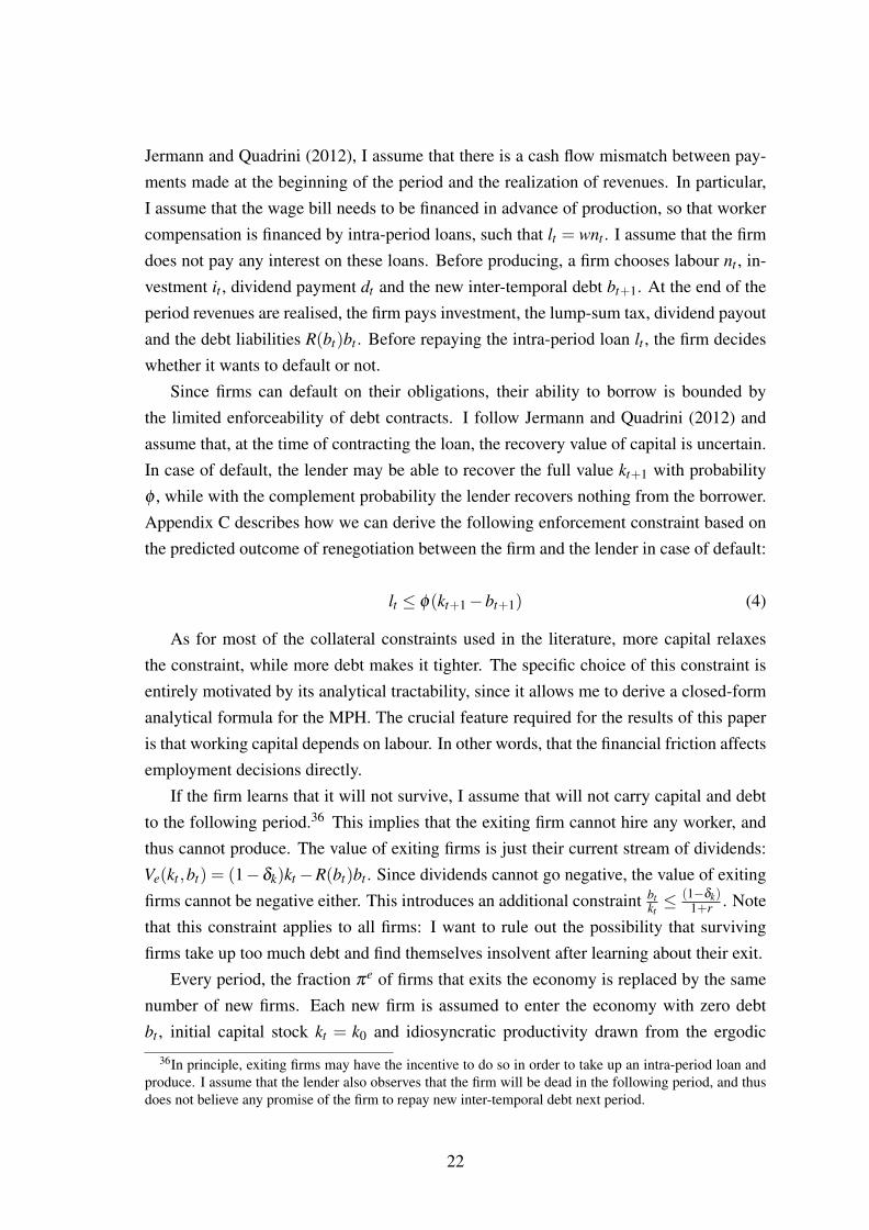
First, the model generates a distribution of MPHs, as shown in figure 3. φ determinesthe lower bound of positive propensities, as can be seen in equation (11). 68% of the firmsin the calibrated model display a positive MPH; the largest firm-level MPH is 0.90. Theshare of constrained firms may seem high; the implied share of firms not paying dividends,however, seems in line with existing evidence, especially given the fact that the model is

40To show this, we use the following findings. First, the autocovariance of TFP growth rates is ρ−11+ρ

σ2ε .

Second, the variance of the log of productivity is σ2ε

1−ρ2 . Third, the variance of TFP growth rates is 2σ2ε

1+ρ.

27

calibrated to data heavily skewed towards small and private firms.41

As in the data, small firms have a greater MPH. The correlation with lagged labour is -0.35 and can be visualized in figure 4a. Two forces affect this correlation; first, conditionalon being positive, the MPH is negatively correlated with size, due to the relationship withthe MPL shown in section 5.2. Second, smaller firms are more likely to have a positiveMPH. It is important to notice that firm exit contributes to this finding.42 Nevertheless,even in presence of firm exit, the correlation can become positive under certain calibra-tions, as shown in the following section.

The model also predicts that more leveraged firms have a greater MPH, as found in thedata. The correlation with net leverage ratio is 0.81, and figure 4b shows that there evenexists a cutoff ratio above which all firms have a positive MPH. As noticed for size, the re-lationship between MPH and leverage is sustained through two different channels. On theextensive margin, highly leveraged firms face a binding collateral constraint and thereforeare more likely to display a positive MPH. Conditional on this, more leveraged firms arealso smaller and, most importantly, have a large MPL, which results in greater firm-levelMPH. Finally, higher labour productivity in the model is associated with greater MPH.Indeed, the firms in the model will have a binding working capital collateral constraintwhen their marginal product of labour is greater than the wage.

The properties highlighted in this section refer to the analytical MPH, derived as insection 5.2.43 Appendix E solves the model for different tax shocks and numerically esti-mates the propensities of labour, capital and debt. This highlights two potential channelsof internal propagation. First, when constrained firms increase employment in responseto a positive cash flow shock, they also make more profits and thus have additional dis-posable resources. Second, greater disposable income may induce firms to borrow moreinter-temporally - anticipating a larger wealth in the future - and further propagate theresponse to the shock.44

41Michaely and Roberts (2011) find that 59% of UK private firms do not pay any dividend, while theshare falls to 29% for publicly listed firms. Their sample of private firms, moreover, excludes small andmedium firms.

42Without exit, the model typically displays a firm-level productivity z cutoff, above which firms havea positive MPH. If the endogenous tightness of the financial frictions is weak, the correlation betweenproductivity and size is positive enough that the correlation between size and MPH is also positive.

43In order to check for accuracy, I numerically evaluate the MPH out of a change in the net financial assetb using the policy functions that solve the model. The resulting average MPH at the stationary distributionis also 0.39.

44The effect on labour is ambiguous: on one hand higher inter-temporal debt sustains more capital in-vestment, potentially relaxing the collateral constraint. On the other hand, it crowds out labour by makingthe constraint tighter.

28

Figure 4: MPH heterogeneity in the model

0 0.1 0.2 0.3 0.4 0.5 0.6 0.7 0.8 0.9 1

MPH

0

5

10

15

20

25

30

35

Em

plo

ym

ent

(a) MPH and size

0 0.1 0.2 0.3 0.4 0.5 0.6 0.7 0.8 0.9 1

MPH

-1

-0.8

-0.6

-0.4

-0.2

0

0.2

0.4

0.6

0.8

1

Net le

vera

ge r

atio

(b) MPH and net leverage ratios

Notes: Figures plot simulated data for the sample of surviving firms used to compute the moments in Table 7. Size is measured interms of employment. In panel (a), model-generated employment has been rescaled so that 1 is the mean employment in the model-generated distribution. To be in line with the data, size and net leverage ratios are lagged one period with respect to the MPH, toidentify pre-determined conditions. The contemporaneous correlation between MPH and size is -0.23. See appendix D for furtherdetails.

6.3 Comparative statics

The marginal propensity to hire in the model can be interpreted as a measure of the en-dogenous tightness of the financial frictions. As such, parameters other than those govern-ing the financial friction itself affect the MPH. In this section I focus on four parameters,and discuss their role in affecting the MPH. In particular, I underline how the averageMPH is effectively the result of two channels; an extensive margin, which measures howmany firms in the economy are constrained, and an intensive margin, which quantifiesthe firm-level intensity of the financial constraints.45 Telling these two channels apart isuseful in order to identify the role played by each parameter in affecting the MPH.

Figure 5 shows how the average MPH changes as we change one parameter at a time,and leaving all the others fixed at the values shown in Table 6.

Endowing new entrants with more capital, by the means of increasing χ , is very effec-tive in lowering the average MPH, as can be seen in the first panel. A larger initial capitalstock implies that firms take less time to mature. In other words, more firms accumulateenough wealth - before exiting - to be able to absorb a negative cash flow shock by reduc-ing dividends or taking up more debt: for this reason, their MPH is 0. This channel can bevisualized in the first panel of figure 7: a larger capital endowment of newly born firms isassociated with a lower share of firms with positive MPH. Greater χ , however, also acts

45The intensity of financial constraints can also be expressed as the average MPH for constrained firms.This statistic can be easily backed out dividing the average MPH by the share of firms with positive MPH.The maximum firm-level MPH, shown in figure 6, also gives an idea of the dispersion of the MPH distribu-tion; since the lower bound of the MPH is φ , this allows us to work out the range of propensities.

29

along the intensive margin of the MPH, as shown in Figure 6. Equation 10 shows that theMPH is inversely correlated with the marginal product of labour. In the model, smallerfirms are more likely to have a larger gap between labour productivity and the wage. Thisgap governs the intensity of the employment response to cash flow shocks.

The second panel of Figures 5-7 shows that the exogenous tightness of the collateralconstraint, φ , affects the average MPH through two counteracting forces. On one hand,greater φ increases the lower bound of positive MPH, as can be seen in equation 10,shifting the MPH distribution to the right. Greater φ implies that firms can get a largerintra-period loan for a given future wealth. £1 of additional cash flow will transmit intomore employment given the capacity to borrow more. On the other hand, it reduces theshare of constrained firms because it makes it easier to borrow. In the quantitative exerciseconsidered here, the first effect prevails.

Finally, neither the persistence nor the standard deviation of firm-level productivityplay a quantitatively important role for the average MPH. σε affects the MPH through two,opposite, margins. A larger variance increases the maximum firm-level MPH by actingthrough the marginal product of labour. On the other hand, it may trigger a precautionarysavings motive that reduces the share of constrained firms.

Figure 8 shows how the correlation between MPH and size is affected by the differentparameters. First, it is not always true that economies with a greater average MPH willalso display a more negative relationship between MPH and labour. Second, we noticethat, even in presence of firm exit, the correlation can turn positive if newly born firmsare endowed with a large initial capital stock. We have noticed earlier how entry and exitcan break the relationship between productivity and size; in particular, the smaller thenew entrants the greater the probability they are credit-constrained, since they will nothave enough wealth to sustain the employment growth suggested by their idiosyncraticproductivity.

30

Figu

re5:

Ave

rage

MPH

0.0

50.1

0.1

50.2

0.2

50.3

0.3

50.1

5

0.2

0.2

5

0.3

0.3

5

0.4

0.4

5

Average MPH

(a)E

ntra

nts’

capi

tal(

%),

χ

0.3

0.4

0.5

0.6

0.7

0.1

5

0.2

0.2

5

0.3

0.3

5

0.4

0.4

5

Average MPH

(b)C

redi

tvar

iabl

e,φ

0.5

50.6

0.6

50.7

0.7

50.1

5

0.2

0.2

5

0.3

0.3

5

0.4

0.4

5

Average MPH

(c)P

ersi

sten

ceof

firm

-lev

elpr

oduc

tivity

,ρz

0.0

80.1

0.1

20.1

40.1

5

0.2

0.2

5

0.3

0.3

5

0.4

0.4

5

Average MPH

(d)S

tand

ard

devi

atio

nof

ε,σ

ε

Figu

re6:

Max

imum

firm

-lev

elM

PH

0.0

50.1

0.1

50.2

0.2

50.3

0.3

5

0.5

0.6

0.7

0.8

0.91

1.1

1.2

Maximum firm-level MPH

(a)E

ntra

nts’

capi

tal(

%),

χ

0.3

0.4

0.5

0.6

0.7

0.5

0.6

0.7

0.8

0.91

1.1

1.2

Maximum firm-level MPH

(b)C

redi

tvar

iabl

e,φ

0.5

50.6

0.6

50.7

0.7

5

0.5

0.6

0.7

0.8

0.91

1.1

1.2

Maximum firm-level MPH

(c)P

ersi

sten

ceof

firm

-lev

elpr

oduc

tivity

,ρz

0.0

80.1

0.1

20.1

4

0.5

0.6

0.7

0.8

0.91

1.1

1.2

Maximum firm-level MPH

(d)S

tand

ard

devi

atio

nof

ε,σ

ε

31

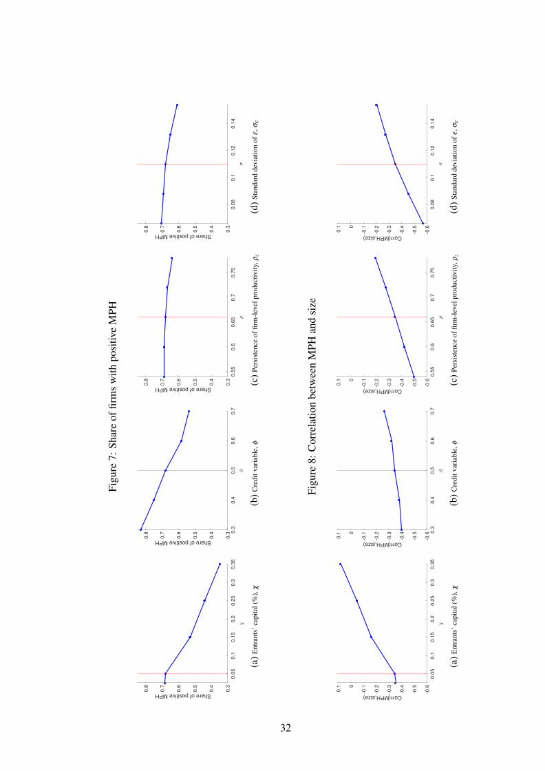
Figu

re7:

Shar

eof

firm

sw

ithpo

sitiv

eM

PH

0.0

50.1

0.1

50.2

0.2

50.3

0.3

50.3

0.4

0.5

0.6

0.7

0.8

Share of positive MPH

(a)E

ntra

nts’

capi

tal(

%),

χ

0.3

0.4

0.5

0.6

0.7

0.3

0.4

0.5

0.6

0.7

0.8

Share of positive MPH

(b)C

redi

tvar

iabl

e,φ

0.5

50.6

0.6

50.7

0.7

50.3

0.4

0.5

0.6

0.7

0.8

Share of positive MPH (c)P

ersi

sten

ceof

firm

-lev

elpr

oduc

tivity

,ρz

0.0

80.1

0.1

20.1

40.3

0.4

0.5

0.6

0.7

0.8

Share of positive MPH

(d)S

tand

ard

devi

atio

nof

ε,σ

ε

Figu

re8:

Cor

rela

tion

betw

een

MPH

and

size

0.0

50.1

0.1

50.2

0.2

50.3

0.3

5-0

.6

-0.5

-0.4

-0.3

-0.2

-0.10

0.1

Corr(MPH,size)

(a)E

ntra

nts’

capi

tal(

%),

χ

0.3

0.4

0.5

0.6

0.7

-0.6

-0.5

-0.4

-0.3

-0.2

-0.10

0.1

Corr(MPH,size)

(b)C

redi

tvar

iabl

e,φ

0.5

50.6

0.6

50.7

0.7

5-0

.6

-0.5

-0.4

-0.3

-0.2

-0.10

0.1

Corr(MPH,size)

(c)P

ersi

sten

ceof

firm

-lev

elpr

oduc

tivity

,ρz

0.0

80.1

0.1

20.1

4-0

.6

-0.5

-0.4

-0.3

-0.2

-0.10

0.1

Corr(MPH,size)

(d)S

tand

ard

devi

atio

nof

ε,σ

ε

32

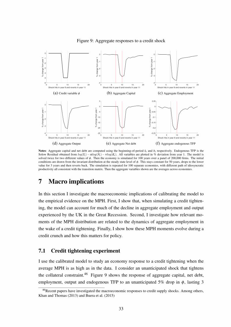
Figure 9: Aggregate responses to a credit shock

0 5 10 15 20

Shock hits in year 8 and reverts in year 11

-6

-5

-4

-3

-2

-1

0

% c

hange fro

m y

ear

1

(a) Credit variable φ

0 5 10 15 20

Shock hits in year 8 and reverts in year 11

-4

-3

-2

-1

0

% c

hange fro

m y

ear

1

(b) Aggregate Capital

0 5 10 15 20

Shock hits in year 8 and reverts in year 11

-4

-3

-2

-1

0

% c

hange fro

m y

ear

1

(c) Aggregate Employment

0 5 10 15 20

Shock hits in year 8 and reverts in year 11

-4

-3

-2

-1

0

% c

hange fro

m y

ear

1

(d) Aggregate Output

0 5 10 15 20

Shock hits in year 8 and reverts in year 11

-25

-20

-15

-10

-5

0

5

% c

hange fro

m y

ear

1

(e) Aggregate Net debt

0 5 10 15 20

Shock hits in year 8 and reverts in year 11

-0.25

-0.2

-0.15

-0.1

-0.05

0

0.05

% c

hange fro

m y

ear

1

(f) Aggregate endogenous TFP

Notes: Aggregate capital and net debt are computed using the beginning-of-period kt and bt respectively. Endogenous TFP is theSolow Residual obtained from log(Yt)−αlog(Nt)− ν log(Kt). All variables are plotted in % deviation from year 1. The model issolved twice for two different values of φ . Then the economy is simulated for 100 years over a panel of 200,000 firms. The initialconditions are drawn from the invariant distribution at the steady state level of φ . This stays constant for 50 years, drops to the lowervalue for 3 years and then reverts back. The simulation is repeated for 100 separate economies, with different path of idiosyncraticproductivity all consistent with the transition matrix. Then the aggregate variables shown are the averages across economies.

7 Macro implications

In this section I investigate the macroeconomic implications of calibrating the model tothe empirical evidence on the MPH. First, I show that, when simulating a credit tighten-ing, the model can account for much of the decline in aggregate employment and outputexperienced by the UK in the Great Recession. Second, I investigate how relevant mo-ments of the MPH distribution are related to the dynamics of aggregate employment inthe wake of a credit tightening. Finally, I show how these MPH moments evolve during acredit crunch and how this matters for policy.

7.1 Credit tightening experiment

I use the calibrated model to study an economy response to a credit tightening when theaverage MPH is as high as in the data. I consider an unanticipated shock that tightensthe collateral constraint.46 Figure 9 shows the response of aggregate capital, net debt,employment, output and endogenous TFP to an unanticipated 5% drop in φ , lasting 3

46Recent papers have investigated the macroeconomic responses to credit supply shocks. Among others,Khan and Thomas (2013) and Buera et al. (2015)

33

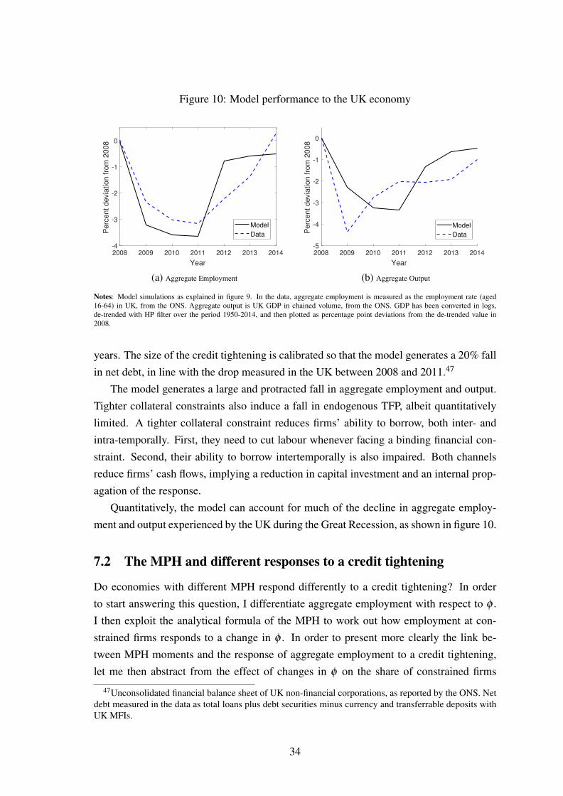
Figure 10: Model performance to the UK economy

2008 2009 2010 2011 2012 2013 2014

Year

-4

-3

-2

-1

0

Perc

ent devia

tion fro

m 2

008

Model

Data

(a) Aggregate Employment

2008 2009 2010 2011 2012 2013 2014

Year

-5

-4

-3

-2

-1

0

Perc

ent devia

tion fro

m 2

008

Model

Data

(b) Aggregate Output

Notes: Model simulations as explained in figure 9. In the data, aggregate employment is measured as the employment rate (aged16-64) in UK, from the ONS. Aggregate output is UK GDP in chained volume, from the ONS. GDP has been converted in logs,de-trended with HP filter over the period 1950-2014, and then plotted as percentage point deviations from the de-trended value in2008.

years. The size of the credit tightening is calibrated so that the model generates a 20% fallin net debt, in line with the drop measured in the UK between 2008 and 2011.47

The model generates a large and protracted fall in aggregate employment and output.Tighter collateral constraints also induce a fall in endogenous TFP, albeit quantitativelylimited. A tighter collateral constraint reduces firms’ ability to borrow, both inter- andintra-temporally. First, they need to cut labour whenever facing a binding financial con-straint. Second, their ability to borrow intertemporally is also impaired. Both channelsreduce firms’ cash flows, implying a reduction in capital investment and an internal prop-agation of the response.

Quantitatively, the model can account for much of the decline in aggregate employ-ment and output experienced by the UK during the Great Recession, as shown in figure 10.

7.2 The MPH and different responses to a credit tightening

Do economies with different MPH respond differently to a credit tightening? In orderto start answering this question, I differentiate aggregate employment with respect to φ .I then exploit the analytical formula of the MPH to work out how employment at con-strained firms responds to a change in φ . In order to present more clearly the link be-tween MPH moments and the response of aggregate employment to a credit tightening,let me then abstract from the effect of changes in φ on the share of constrained firms

47Unconsolidated financial balance sheet of UK non-financial corporations, as reported by the ONS. Netdebt measured in the data as total loans plus debt securities minus currency and transferrable deposits withUK MFIs.

34

and postpone its analysis. I therefore consider a (approximate) sensitivity of aggregateemployment to φ , which can be decomposed as follows in the spirit of Olley and Pakes(1996):48

∂N∂φ≈∫ ni

φ 2 MPHidi =1

φ 2 [E(MPH)E(n)+COV (MPH,n))di (12)

Two forces are in place. Greater average MPH, ceteris paribus, implies a greatersensitivity of aggregate employment to φ . As discussed before, this depends, in turn, onboth how many firms are constrained and the firm-level intensity of the financial friction.In an economy in which employment choices are more often and more severely impairedby borrowing restrictions, a further tightening of credit conditions will intuitively result ingreater employment losses. On the other hand, aggregate employment will respond moreto a credit tightening the more positive the covariance between employment and the MPH.When larger firms are more severely affected by financial frictions, a tightening of creditconditions will cause larger employment losses due to the greater employment share ofthese firms. As shown in figures 5-8, the two forces often go in the opposite direction.

The analysis so far has clearly pointed at the relevance of MPH statistics for the re-sponse of aggregate employment to a credit tightening. Nevertheless, it abstracts from theresponse of the share of constrained firms, it is necessarily applied to local changes in φ

and focuses on the response upon impact. I now compare numerically how economiesthat differ with respect to their average MPH respond differently to the credit tighteningshock considered in figure 9. This exercise crucially depends on the way in which dif-ferent values of the average MPH are achieved. I decide to focus on χ , given that thequantitative properties of the MPH are particularly sensitive to this parameter.

Figure 11 shows the impulse response functions for three different economies. Thesolid black line refers to the benchmark calibrated economy with an average MPH of0.39. The second economy, in red, achieves an average MPH of 0.23 by the means ofincreasing χ to 25%.49 In the dashed blue-line economy firms never exit: the averageMPH is 0.07.

Aggregate responses are clearly ordered by the average MPH of the economy. Thedrop in aggregate employment upon impact can be tied to the analytical analysis pursuedat the beginning of this section. A greater average MPH implies, ceteris paribus, a strongerresponse of aggregate employment. The benchmark economy, however, has also the low-est covariance between employment and the MPH. According to equation 12 this shouldimply, ceteris paribus, a weaker response of aggregate employment. The former effectdominates in the aggregate. The blue economy, for instance, has a covariance of 0.0178,

48Full derivation in Appendix F.49This implies that the entrants’ employment size is 37% of the average.

35

Figure 11: Aggregate responses to a credit shock: different MPH by changing χ

0 5 10 15 20

Shock hits in year 8 and reverts in year 11

-6

-5

-4

-3

-2

-1

0

% c

hange fro

m y

ear

1

(a) Credit variable φ

0 5 10 15 20

Shock hits in year 8 and reverts in year 11

-4

-3

-2

-1

0

1

% c

hange fro

m y

ear

1

(b) Aggregate Capital

0 5 10 15 20

Shock hits in year 8 and reverts in year 11

-4

-3

-2

-1

0

1

% c

hange fro

m y

ear

1

(c) Aggregate Employment

0 5 10 15 20

Shock hits in year 8 and reverts in year 11

-4

-3

-2

-1

0

1

% c

hange fro

m y

ear

1

(d) Aggregate Output

0 5 10 15 20

Shock hits in year 8 and reverts in year 11

-200

-150

-100

-50

0

50

% c

hange fro

m y

ear

1

(e) Aggregate Net debt

0 5 10 15 20

Shock hits in year 8 and reverts in year 11

-0.25

-0.2

-0.15

-0.1

-0.05

0

0.05

% c

hange fro

m y

ear

1

(f) Aggregate endogenous TFP

MPH = 0.07 MPH = 0.23 MPH = 0.39

Notes: Aggregate capital and net debt are computed using the beginning-of-period kt and bt respectively. Endogenous TFP is theSolow Residual obtained from log(Yt)−αlog(Nt)− ν log(Kt). All variables are plotted in % deviation from year 1. The model issolved twice for two different values of φ . Then the economy is simulated for 100 years over a panel of 200,000 firms. The initialconditions are drawn from the invariant distribution at the steady state level of φ . This stays constant for 50 years, drops to the lowervalue for 3 years and then reverts back. The simulation is repeated for 100 separate economies, with different path of idiosyncraticproductivity all consistent with the transition matrix. Then the aggregate variables shown are the averages across economies.

compared with -0.0058 in the benchmark: this is not enough, however, to overturn thefact that the average MPH is more than 5 times lower than in the black economy. In turn,aggregate employment falls by 1.6% upon impact when the MPH is low, and 3.3% whenit is high. Most importantly, note that only the benchmark economy is in line with thedata with regard to the covariance between MPH and firm size. The alternative calibra-tions shown in the figure, in contrast, imply that larger firms will exhibit greater marginalpropensities to hire, at odds with the empirical evidence shown in Table 5. We can alsouse equation 12 and the numerical impulse responses to back out the portion of the initialdrop in aggregate employment accounted for by the firms becoming constrained after thecredit shock. This is 7.4% in the black economy, 1.8% in the intermediate and 10% in thelow-MPH economy.50

Economies with different average MPH also display different aggregate dynamics,beyond the response upon impact. When the MPH is low, a credit tightening implies

50It should be noted, however, that part of this gap may be due to the inaccuracy of the first-order Taylorapproximation.

36

a short-lived drop of employment and capital - note that they both start recovering dur-ing the crisis - and an overshooting when ordinary credit conditions are restored. Netdebt drops substantially and absorbs part of the credit tightening. The higher the aver-age MPH, the larger both the drop of employment and capital and its persistence; in thebenchmark economy, the credit tightening propagates implying that, 5 years after the endof the credit contraction, aggregate output is still 0.4% below its pre-crisis levels. A creditsupply shock implies a drop in endogenous TFP, as also found by Khan and Thomas(2013): tighter financial frictions imply stronger misallocation of resources. In particular,productive firms with little wealth take more time to expand towards their optimal size.The greater the MPH, the stronger this effect: TFP drops 4 times more in the benchmarkeconomy than in the low-MPH economy.

This section has shed some light on the interaction between the MPH and the ag-gregate dynamics following a credit tightening. While simulation exercises suggest thateconomies with greater average MPH display a larger and more prolonged fall in aggre-gate employment, this may be specific to the way in which different MPH moments havebeen achieved - i.e.: by changing χ . Moreover, equation 12 clearly shows that additionalmoments as the covariance between MPH and size are important. Analysing in greaterdetail the features of the MPH distribution seems a promising avenue to better understandthe transmission mechanism of credit supply shocks onto aggregate employment and isleft to future research.

7.3 The MPH during a credit tightening

What happens to the MPH during a credit crisis? In section 6.3 we have seen how φ

affects the marginal propensity to hire along two opposite margins. When the collateralconstraint is tighter, more firms will be at the binding constraint, which implies that theshare of firms with positive MPH will increase. This is shown in figure 12b. On theother hand, φ is negatively correlated with the firm-level analytical MPH, as shown inequation 10. Indeed, φ measures the firm’s capacity to leverage up on future wealth andborrow intra-temporally. For a given £1 of additional cash flow, firms will be able toborrow less the lower φ , thus transmitting in fewer additional employment expendituresand therefore a lower MPH. This effect prevails on average, implying the small dip in theaverage MPH seen in figure 12a.

This finding suggests that stabilisation policies in the form of uniform lump-sum trans-fers may be less effective in boosting aggregate employment during credit tightening pe-riods. While the analytical MPH abstracts from the effect of lump-sum cash flow shockson changes in the constraint status of the firm, it is not clear ex ante why the size of thesetransfers should have differential effects along this margin during a credit tightening pe-

37

Figure 12: The MPH in a credit crisis

0 5 10 15 20

Shock hits in year 8 and reverts in year 11

0.37

0.375

0.38

0.385

0.39

0.395

0.4

Ave

rag

e M

PH

(a) Average MPH

0 5 10 15 20

Shock hits in year 8 and reverts in year 11

67

68

69

70

71

72

% o

f firm

s w

ith

po

sitiv

e M

PH

(b) Share of firms with positive MPH

0 5 10 15 20

Shock hits in year 8 and reverts in year 11

-0.25

-0.245

-0.24

-0.235

-0.23

-0.225

-0.22

Co

rr(M

PH

,em

plo

ym

en

t)

(c) Correlation between MPH and size

0 5 10 15 20

Shock hits in year 8 and reverts in year 11

0.009

0.0095

0.01

0.0105

0.011

0.0115

0.012

Se

nsitiv

ity o

f a

gg

reg

ate

em

plo

ym

en

t to

(d) Sensitivity of aggregate employment to φ

Notes: Notes to figure 9 apply. The correlation plotted in 12c is contemporaneous. Panel (d) shows the approximate sensitivity ofaggregate employment to φ , as computed in equation 12

riod. A credit crunch makes also more mildly negative the correlation between MPH andsize, as shown in figure 12c. This suggests that policies targeted at small firms should bemore effective during this type of recessions. Finally, in figure 12d I plot the approximateresponse of aggregate employment to φ computed using equation (16). In this context,we can interpret this statistic from a policy perspective. Suppose the policymaker wasable to affect the tightness of financial frictions by acting on φ , this statistic would givethe approximate sensitivity of aggregate employment, with the usual caveat of abstract-ing from the response of the extensive margin. This sensitivity falls slightly during thecredit tightening period. The fall in the average MPH, in aggregate employment, andin the covariance between employment and MPH all push down the sensitivity during acredit crunch. φ itself, however, has fallen, implying that the drop is less pronounced.As before, this finding suggests that policies aimed at acting directly on the tightness offinancial frictions may be less effective during credit crunches.

38

8 Conclusions

The interaction between firm-level financial constraints and employment decisions hasreceived a lot of attention following the Great Recession and the financial crisis. In thispaper, I first empirically show that financial constraints matter for firms’ employmentdecisions. I exploit the idea that, when financial constraints bind, a firm adjusts its em-ployment in response to cash flow shocks. I use a novel combination of three large datasets in the UK and a new source of variation to estimate this response, which I label theMarginal Propensity to Hire. In particular, I exploit the changes to a UK tax based on aperiodically estimated value of the property occupied by the firm. I find that, on average,for every £1 of additional cash flow, 39 pence are spent on employment. Moreover, smalland leveraged firms display a greater MPH. I then build a model of firm dynamics andfinancial frictions and calibrate it to macro and micro features of the data, including theaverage MPH. The model sheds light on the nature of employment - cash flow sensitivitiesand can replicate the empirical evidence on the cross-sectional heterogeneity of the MPH.The empirical evidence on the MPH and its distribution can be used as a tool to informquantitative macro models. In this paper I show that, simulating a tightening of creditconditions, the calibrated model can account for much of the decline in aggregate outputand employment observed in the wake of the financial crisis. In ongoing work, I am us-ing the theoretical apparatus and its link with the empirical findings to tackle another bigmacro question, namely how much misallocation do financial frictions create.

39

References

Almeida, Heitor, Murillo Campello, and Michael S Weisbach, “The cash flow sensi-tivity of cash,” Journal of Finance, 2004, 59 (4), 1777–1804.

Anyadike-Danes, M, K Bonner, and M Hart, “Job Creation and Destruction in the UK:1998-2010,” BIS Analytical Report, 2011.

Bassetto, Marco, Marco Cagetti, and Mariacristina De Nardi, “Credit crunches andcredit allocation in a model of entrepreneurship,” Review of Economic Dynamics, 2015,18 (1), 53–76.

Benmelech, Efraim, Nittai K Bergman, and Amit Seru, “Financing labor,” 2015.

Bernanke, Ben S, Mark Gertler, and Simon Gilchrist, “The financial accelerator in aquantitative business cycle framework,” Handbook of macroeconomics, 1999, 1, 1341–1393.

Boeri, Tito, Pietro Garibaldi, and Espen R Moen, “Financial constraints in searchequilibrium: Mortensen Pissarides meet Holmstrom and Tirole,” Labour Economics,2017, Forthcoming.

Bond, Stephen, Kevin Denny, John Hall, and William McCluskey, “Who pays busi-ness rates?,” Fiscal Studies, 1996, 17 (1), 19–35.

Bond, Stephen R and Mans Soderbom, “Conditional investment–cash flow sensitivitiesand financing constraints,” Journal of the European Economic Association, 2013, 11

(1), 112–136.

Bracke, Philippe, “House prices and rents: Microevidence from a matched data set inCentral London,” Real Estate Economics, 2015, 43 (2), 403–431.

Brav, Omer, “Access to capital, capital structure, and the funding of the firm,” Journal of

Finance, 2009, 64 (1), 263–308.

Buera, Francisco J, Roberto N Fattal Jaef, and Yongseok Shin, “Anatomy of a creditcrunch: from capital to labor markets,” Review of Economic Dynamics, 2015, 18 (1),101–117.

Cahuc, Pierre, Stephane Carcillo, and Thomas Le Barbanchon, “Do hiring creditswork in recessions? Evidence from France,” 2014.

40

Chaney, Thomas, David Sraer, and David Thesmar, “The collateral channel: How realestate shocks affect corporate investment,” American Economic Review, 2012, 102 (6),2381–2409.

Chodorow-Reich, Gabriel, “The employment effects of credit market disruptions: Firm-level evidence from the 2008–9 financial crisis,” Quarterly Journal of Economics, 2013,129 (1), 1–59.

Davis, Steven J and John Haltiwanger, “Gross job creation, gross job destruction, andemployment reallocation,” Quarterly Journal of Economics, 1992, 107 (3), 819–863.

Farre-Mensa, Joan and Alexander Ljungqvist, “Do measures of financial constraintsmeasure financial constraints?,” Review of Financial Studies, 2016, 29 (2), 271–308.

Fazzari, Steven M, R Glenn Hubbard, Bruce C Petersen, Alan S Blinder, andJames M Poterba, “Financing constraints and corporate investment,” Brookings pa-

pers on economic activity, 1988, 1988 (1), 141–206.

Gertler, Mark and Simon Gilchrist, “Monetary policy, business cycles, and the behaviorof small manufacturing firms,” Quarterly Journal of Economics, 1994, 109 (2), 309–340.

Giroud, Xavier and Holger M Mueller, “Firm leverage, consumer demand, and em-ployment losses during the Great Recession,” Quarterly Journal of Economics, 2017,132 (1), 271–316.

Guner, Nezih, Gustavo Ventura, and Yi Xu, “Macroeconomic implications of size-dependent policies,” Review of Economic Dynamics, 2008, 11 (4), 721–744.

Hubbard, R Glenn, “Capital-Market Imperfections and Investment,” Journal of Eco-

nomic Literature, 1998, 36, 193–225.

Jermann, Urban and Vincenzo Quadrini, “Macroeconomic effects of financial shocks,”American Economic Review, 2012, 102 (1), 238–271.

Kaplan, Steven N and Luigi Zingales, “Do investment-cash flow sensitivities provideuseful measures of financing constraints?,” Quarterly journal of economics, 1997, 112

(1), 169–215.

Khan, Aubhik and Julia K Thomas, “Credit shocks and aggregate fluctuations in aneconomy with production heterogeneity,” Journal of Political Economy, 2013, 121 (6),1055–1107.

41

Mehrotra, Neil and Nicolas Crouzet, “Small and Large Firms over the Business Cycle,”in “2017 Meeting Papers” number 600 Society for Economic Dynamics 2017.

Mian, Atif and Amir Sufi, “What explains the 2007–2009 drop in employment?,” Econo-

metrica, 2014, 82 (6), 2197–2223.

Michaels, Ryan, Beau Page, and Toni M Whited, “Labor and capital dynamics underfinancing frictions,” 2016.

Michaely, Roni and Michael R Roberts, “Corporate dividend policies: Lessons fromprivate firms,” Review of Financial Studies, 2011, 25 (3), 711–746.

Moscarini, Giuseppe and Fabien Postel-Vinay, “The contribution of large and smallemployers to job creation in times of high and low unemployment,” American Eco-

nomic Review, 2012, 102 (6), 2509–2539.

Office for National Statistics, “Business Structure Database, 1997-2017: Secure Ac-cess,” 9th Edition, 2017, (SN 6697).

Olley, G. Steven and Ariel Pakes, “The Dynamics of Productivity in the Telecommuni-cations Equipment Industry,” Econometrica, 1996, 64 (6), 1263–1297.

Quadrini, Vincenzo, “Financial frictions in macroeconomic fluctuations,” 2011.

Rauh, Joshua D, “Investment and financing constraints: Evidence from the funding ofcorporate pension plans,” Journal of Finance, 2006, 61 (1), 33–71.

Riddick, Leigh A and Toni M Whited, “The corporate propensity to save,” Journal of

Finance, 2009, 64 (4), 1729–1766.

Schoefer, Benjamin, “The financial channel of wage rigidity.” PhD dissertation, HarvardUniversity 2015.

Strebulaev, Ilya A and Toni M Whited, “Dynamic models and structural estimation incorporate finance,” Foundations and Trends in Finance, 2012, 6 (1–2), 1–163.

Tauchen, George and Robert Hussey, “Quadrature-based methods for obtaining ap-proximate solutions to nonlinear asset pricing models,” Econometrica, 1991, pp. 371–396.

Zetlin-Jones, Ariel and Ali Shourideh, “External financing and the role of financialfrictions over the business cycle: Measurement and theory,” Journal of Monetary Eco-

nomics, 2017.

42

Appendix

A The data

A.1 Data description and construction

This paper uses information primarily from three data sources, which I describe in thissection: The Business Structure Database (Office for National Statistics (2017)), the Rat-ing List and Summary Valuations compiled by the Valuation Office Agency and the Fi-nancial Analysis Made Easy (FAME) of the Bureau van Dijk.

Quoting the UK Data Service Catalogue description, “The Business Structure Database(BSD) is derived primarily from the Inter-Departmental Business Register (IDBR), whichis a live register of data collected by HM Revenue and Customs via VAT and Pay As YouEarn (PAYE) records. The IDBR data are complimented with data from ONS businesssurveys. If a business is liable for VAT and/or has at least one member of staff regis-tered for the PAYE collection tax system, then the business will appear on the IDBR (andhence in the BSD). In 2004, it was estimated that the businesses listed on the IDBR ac-counted for 99 per cent of economic activity in the UK. Only very small businesses, suchas self-employed, were not found on the IDBR.”

The BSD is created by the ONS virtual Micro-data Laboratory (VML); every year,a snapshot of the IDBR is taken around April, and the captured point-in-time data aresupplied to the VML by the following September. The reporting period is generally thefinancial year. For example, the 2000 BSD file is produced in September 2000, usingdata captured from the IDBR in April 2000. The data will typically reflect the financialyear of April 1999 to March 2000. Employment information for the vast majority offirms, for instance, is updated on the IDBR using quarterly PAYE information. However,the ONS may, during this time, update the IDBR with data on companies from its ownbusiness surveys. I follow the literature, such as Anyadike-Danes et al. (2011), and definethe BSD variables with respect to the named year of the snapshot. The data are dividedinto enterprises and local units. The enterprise is defined as “the smallest combinationof legal units that is an organisational unit producing goods or services, which benefitsfrom a certain degree of autonomy in decision-making, especially for the allocation of itscurrent resources”. A local unit is “an enterprise or part thereof (e.g.: a workshop, factory,warehouse, office, mine or depot).”; “(...) to qualify as a local unit, a business entitymust only consist of one site at a mailing address”. For each business, data are availableon employment, turnover, foreign ownership, legal status, industrial activity based onStandard Industrial Classification (SIC), year of birth and death, as well as postcodes forboth enterprises and local units. Turnover information is available only at the enterprise

43

level. Within the IDBR, every local unit and enterprise is given its own, unique referencenumber when it enters onto the IDBR which remains unique to that business whilst itremains, in the same form, on the register. Given its confidential nature, the BusinessStructure Database can be accessed only through the UK Data Service Secure Lab.

Tax liabilities are calculated using information on Rating Lists and Summary Valu-ations, as provided by the Valuation Office Agency. The VOA compiles and maintainsthe rating list of rateable values for around 1.9 million non-domestic properties in Eng-land and Wales. About 80% of these properties have a summary valuation. I considerinformation drawn from the 2005 and 2010 rating lists, with summary valuations infor-mation for 2010. The data contains information on the adopted rateable value, the addressof the property, date information on alteration to the rateable value and its effectiveness,the property category type and description, the size of the property measured in squaremeters, the adopted pounds per square meter rateable value and the valuation scheme ref-erence number. Part of the tax data is live, which means that any physical change to theproperty after the revaluation will over-write the existing information. I try to account forthis while matching the data by creating two comparable datasets. This will not be anissue in the empirical analysis, since the specific sample considered contains non-updatedinformation at 2010 for all properties. For the tax data, I retain the properties that havenon-missing rateable values before and after 2010. This excludes properties that werebuilt, or closed, after the revaluation. For the BSD local unit data, I start by retaining localunits in England and Wales, to be in line with the business rates. I then keep local unitsthat did not change postcode sector around the revaluation,51 and that are live between2009 and 2011. I also exclude local units that die after 2012 without changing postcode,interpreting this as a property closure too. I break each side of the sample into two groups,depending on whether each full postcode unit has only one property (local unit) or more.I then proceed to match those sample groups. In some cases, one local unit is associatedwith more properties in the same postcode. Local units are defined as places where eco-nomic activity is carried out by one or more persons work; VOA properties, instead, donot require any employee. I therefore create a mapping between the SIC industry code ofthe local unit and the category type of the property, allowing for groups of properties thatare likely to be part of the same local unit.52 The mapping between industry codes andproperty types is also used for postcodes with multiple local units and multiple properties,or to check ex post the correctness of the matching.

51I allow for small changes in the postcode unit, since this allows me to match over postcode sector tooat a later stage. This may be coding error, change in the coding of the last letter of a postcode, or genuinerelocations ”next door”. In unreported results, I check that the estimated average MPH is unaffected whendropping these few occurrences.

52For example any property and its car park/ATMs/garages, or a school with its sport ground.

44

In order to allow for measurement error of postcode units, I repeat the same strategy atthe postcode sector level, adding a small number of additional matches. The final sampleconsists of roughly 175,000 observations. The sample is then merged with firm-level in-formation from the BSD, using the unique identifier that links local units and enterprises.There are 135,139 firms in the sample. I then exclude central government bodies and lo-cal authority establishments, establishments with 0 employees, properties with a rateablevalue of £0. To be in line with rental method for revaluation, as explained in section 2,I keep only the properties reporting a valuation scheme reference number. Moreover, Iexclude all properties whose category - i.e.: property type - may be valued with methodsother than the rental method. 53 I then exclude the properties incurring in material changeof circumstances between 1 April 2010 and 2012. Indeed, firms have the possibility toreduce their tax bill by changing the features of the property and then reporting a materialchange of circumstances at the Valuation Office Agency.54 This may imply a change inemployment due to the complementarity with fixed assets and following a response toa change in the user cost of capital; since, instead, I am interested in the balance sheetchannel of cash flow shocks, I exclude this possibility. In the data, it is not possible toobserve directly whether a material change of circumstances took place. Nevertheless,I follow the Rating Manual, Volume 2, Section 5, Paragraph 6 and assume that any ef-

fective date beyond 2010 is deemed to be the date the circumstances arose that requiredthe list to be altered. I also drop all properties incurring in an alteration to its pre-2010rateable value taking place after 2010. This is typically the result of overdue resolutionof appeals or retroactive changes to the tax bill. Finally, I drop the establishments thatchanged enterprise between 2009 and 2011, and the construction sector (UKSIC 41100-43999), given its special nature when it comes to a property tax. The sample now consistsof 82,506 establishment-tax observations. The employment variable used in the analysisexcludes business owners - thus measuring only the number of employed staff. To protectthe results from the effect of the outliers, I trim the dependent variables at the 1st and 99thpercentiles. I also drop the upper and lower 0.75 percent of the scaled tax shock. Resultsare robust to 1 percentile trimming of the tax shock.

When calculating the pound-for-pound MPH, I rescale the employment changes byan annual wage of £21,024. According to the Annual Survey of Hours and Earnings, in

53Fish farms and public religious worship halls may be exempted upon request to the local authority.The other valuation methods are: contractors’ basis, revenue and expenditure method, fair maintainablereceipts, agreed valuation, special treatment (e.g.: football stadia). The relevant information can be foundin the Valuation Office Agency Rating Manual, Volume 5. I also exclude all the categories that may bevalued through a national, rather than local, scheme.

54Material change of circumstances typically involve matters affecting the physical state or physicalenjoyment of the hereditament and the category of occupation of hereditament (Rating Manual Volume 2Section 5). While potentially still working through the balance sheet, the cash flow shock may depend onthe marginal product of capital and driven by other reasons such as endogenous location choices.

45

Table 8: Descriptive statistics

Mean Std. Dev. Median Mean (>0)

∆2009,10T (% of Sales2008) − 0.05 0.7 -0.03 0.4∆2009,11Emp (% of Sales2008) 1.4 15 0 17Emp2008 103 2,054 5Sales2008 (Th GBP) 17,364 541,400 250

Note: Moments calculated from the sample of 63,242 observations in Table 1. Median values are averages around the median whenthere are less than 10 observations taking the median value.

April 2010 median gross weekly earnings for all employees were £404, which gives therescaling wage if multiplied by 52 weeks. It seems sensible to consider both part-time andfull-time employees when calculating the wage, especially given the very large number ofsmall firms in the sample. Moreover, small firms typically pay lower wages and employmore part-time employees, as shown in the 2016 Annual Survey of Hours and Earnings;this may lead to overestimation of the pound-for-pound MPH.55 On the other hand, itmay underestimate the MPH since gross earnings slightly underplay firms’ labour costs.Gross weekly earnings include regular pay - gross of income tax and employee Nationalinsurance contributions -, overtime pay and one-off bonuses, but exclude employer Na-tional insurance contributions, employer contributions to pensions schemes, benefits inkind, signing-on fees and stock options not paid through payroll.

Table 8 shows the descriptive statistics for the sample used in Table 1, while Figure13 the distribution of the scaled tax shocks.

A.2 Robustness to the average MPH

The analysis done in section 4 constructs tax shocks using tax liabilities calculated by theauthor. A few important comments are worth making, which will be the object of thissection. The tax liability is calculated by multiplying the relevant rateable value by themultiplier. There are two main multipliers, one for Wales and one for England. I referto section 2 for the description of how multipliers are updated every year. I then make aseries of adjustments concerning the multipliers. The City of London authority chargedan additional 0.4p for the properties in its area. Since the 1st April 2010, the Greater Lon-don Authority introduced a 2p additional levy on the multiplier, for rateable values over£55,000. Small properties, in England only, benefit from a lower multiplier, depending

55The median weekly earnings at micro firms (less than 10 employees) was 64% of the overall median in2016. Part-time employees at those firms earned even less (35%). At the other extreme of the distribution,full-time employees at large firms earned 29% more than the overall median.

46

Figure 13: The distribution of tax shocks

Note: Distribution of ∆2009,10T as of column III of Table 1.

on the rateable value of their property and the sum of all rateable values at the business.56

The small business multiplier is automatically assumed, according to the rateable value ofthe property, since 2010 revaluation; the VOA then checks if the conditions of eligibilityapply to the ratepayer. In the main analysis, I compute small business multipliers. Col-umn I of Table 9 shows that the results are unchanged if I get rid of the small businessmultipliers when constructing the tax liabilities.

A number of reliefs are in place, which may affect the business rates liability. Thesmall business rates relief is subject to the same conditions of the small business multi-plier, but businesses need to explicitly apply for this to the relevant local authority. Thedataset does not have the necessary information to take this into account, since businessesare not matched with all the properties they occupy and, moreover, there is no public in-formation on whether the business rates relief has been granted. Restricting the analysisto the observations that are certainly not affected by the SBRR reduces the sample size bymore than half but delivers similar results.

After the 2010 revaluation, a transitional relief was introduced in England only, aimedat phasing in sharp changes in the tax bills. The VOA set out the limits on the percentage

56To qualify for the small business multiplier, the ratepayer needed to fulfil the following criteria forthe 2005 (2010) rating list: the ratepayer must occupy only one business in England or must occupy oneproperty in England and other additional business properties, such that the main property has a rateablevalue less than £15,000 (£18,000) and £21,500 (£25,500) in London, each additional business property hasa rateable value less than £2,200 (£2,600) and the combined value is less than the threshold.

47

Table 9: Robustness

∆2009,11Emp (∆2009,11Emp−∆2006,08Emp)

(I) (II) (III) (IV) (V)

∆2009,10T −0.38∗∗∗ −0.39∗∗∗ −0.54∗∗

(0.13) (0.11) (0.21)

1st year relieved ∆T −0.57∗∗∗

(0.18)

5-year relieved ∆T −0.10∗∗∗

(0.03)

Observations 63,242 63,242 63,242 62,700 54,703R2 0.01 0.01 0.01 0.01 0.01

Note: Standard errors (in parentheses) are clustered at the postcode area level. ∗, ∗∗ and ∗∗∗ denote significance at the 10%, 5% and1% level, respectively. Same notes and controls of column III of Table 1 apply.

by which the rates bill can increase or decrease every year.57 The property is consideredinto the scheme until the true tax liability does not exceed the relieved tax bill. ColumnII shows the marginal propensity to hire calculated out of the first-year cash flow shockinduced by the revaluation, after the transitional relief is considered. The coefficient isclearly larger than in the main analysis, because some firms know that they will face alarger tax shock in the future. In column III, I calculate the 5-year present value of taxshocks. This sums the relieved cumulative tax shocks for the following 5 years, withrespect to the pre-revaluation tax liability.5859 The coefficient is still slightly larger thanone fifth of the average MPH, suggesting that calculating the tax shocks before any reliefeffectively underestimates the MPH.

Excluding the financial and insurance activities (section K, UKSIC 2007 codes 64110-66300) and the public administration and defence (section O, UKSIC 2007 codes 84110- 84300) does not affect the estimates, as shown in Column IV. The estimated MPH isunchanged if excluding also the real estate activities (section L, UKSIC 2007 codes 68100

57The scheme was originally devised to last 5 years. Limits to the reductions of tax bills were introducedto partly fund the scheme. Different limits apply for small and large properties, classified as such dependingon their rateable value and whether they are in London. Year on year increases were limited to 5, 7.5, 10,15 and 15 per cent for small properties, 12.5, 17.5, 20, 25 and 25 per cent for large properties. Decreaseswere limited to 20, 30, 35, 55 and 55 per cent for small properties and 4.6, 6.7, 7, 13 and 13 per cent forlarge properties.

58Note that this is meant to be a calculation made upon revaluation impact by a potential business. Theex-post actual sum of tax changes will be different, since business rates multipliers are adjusted every yearin line with RPI.

59The present value as a share of firm sales has an average of -0.3%, 3.0% of standard deviation and ison average 1.5% conditional on being positive.

48

- 68320).Finally, in column V I estimate the pound-for-pound sensitivity of the change in net

hiring to a cash flow shock. In order to do so, I net the 2009-11 employment changewith the 2006-08 employment change. The estimated coefficient is slightly larger thanthe benchmark, in line with the fact that there is a mild positive correlation between therevaluation and pre-2008 employment changes.

In unreported findings, I check that the results are robust to the anticipation of futurechoices along the extensive margin, such as establishment closures or material change ofcircumstances. 634 establishments in the sample are shut down in 2012: excluding theseobservations leaves the estimated average MPH unchanged. The MPH is even slightlygreater at −0.42∗∗∗ when excluding the establishments relocating in 2012. Finally, thecoefficient is unchanged when excluding the material change of circumstances takingplace in 2012.

A.3 Multiple establishments

The benchmark analysis pursued in this paper retains, for every firm i, the largest (in ab-solute value) establishment-level tax shock. This has the advantage of using explicitly theproperty-level and geographic controls to clean potentially endogenous and anticipatedeffects of the tax shock on employment. On the other hand, firms with multiple estab-lishments will be likely to face an overall tax change that is different from than the oneconsidered in the analysis. The direction of the bias is unclear ex ante, because it dependson the correlation between the different tax shocks faced by each firm i. In this section Ishow that, in practice, this issue does not affect the estimation of the MPH.

First, I show that, by restricting the sample to the firms with only one establishmentbetween 2009 and 2011, as done in Column I of Table 10, the vast majority of obser-vations is kept and the average MPH unchanged. In Column II I re-introduce multiple-establishment firms and estimate the MPH out of the overall tax shock at the firm level(i.e.: the sum across all establishments). This specification may introduce some noisesince the property-level and geographical controls refer to the property associated withthe largest firm-level tax shock. The estimated coefficient is very similar, suggesting thatthe bias introduced by looking only at the largest tax shock (in absolute value) for eachfirm does not systematically affect the estimation.

I then try to quantify the direction of the bias related with multiple establishments. Atthis stage, it is useful to recall that businesses have two ways to overturn a tax change:closing the establishment, or physically changing the property, incurring in a material

49

Table 10: Multiple-establishment firms

∆2009,11Emp

(I) (II) (III)

∆2009,10T −0.40∗∗∗ −0.41∗∗∗

(0.11) (0.11)

Total firm-leveltax change −0.38∗∗∗

(0.11)

Single establishments only X

Number of firms 55,121 63,242 63,242R2 0.01 0.01 0.01

Note: Same notes and controls of column III of Table 1 apply. Standard errors (in parentheses) are clustered at the postcode arealevel, except for column IV in which they are clustered at firm level. ∗, ∗∗ and ∗∗∗ denote significance at the 10%, 5% and 1% level,respectively.

change of circumstances. Both options are excluded by the sampling strategy.60 Reshuf-fling workers across different establishments should not be caused by a tax shock, since itdoes not overturn any tax change, unless a physical change takes place. If the estimatedMPH is really measuring the employment responses out of cash flow shocks, we wouldexpect firms with multiple establishments, and whose total tax shock partly cancels out atthe firm level, to respond less. The analysis performed in Table 1 may also be affected byanother source of bias: for some firms in the sample it is not possible to match all the es-tablishments with the associated tax change at the property level. I investigate both issuesby augmenting specification (1) as follows. First, I add a dummy M that takes 1 if not allfirm i establishments are matched with a tax entry. Second, a dummy O which takes 1 ifthe overall firm tax shock has a different sign than the largest shock ∆2009,10Tj,m. Only0.1% of the firms in the sample have overall offsetting shocks. Finally, I interact bothdummies with ∆2009,10Tj,m.

As shown in Column III, the average MPH is even slightly greater than the benchmarkestimate. All the coefficients associated with the additional variables described above areinsignificantly different from 0. Only firms with at least one establishment not matchedwith the property have, on average, a more positive employment growth. Most impor-tantly, firms with offsetting shocks do not display a systematically different response tothe tax change, providing an additional test for the presence of the cash flow channelwhich I try to quantify.

60Closures and material change of circumstances are ruled out until 2012. In Appendix A.2 I show thatthe coefficient is not affected by employment responses in anticipation of closures or physical changestaking place after 2012.

50

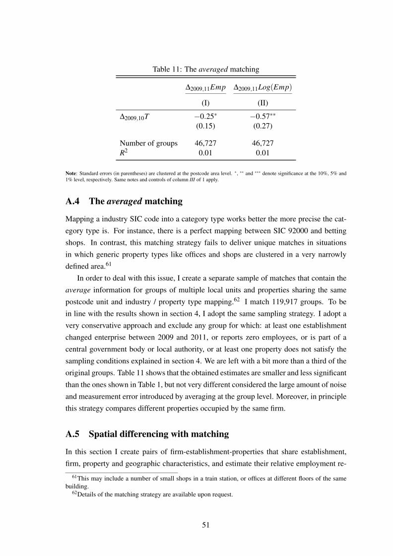
Table 11: The averaged matching

∆2009,11Emp ∆2009,11Log(Emp)

(I) (II)

∆2009,10T −0.25∗ −0.57∗∗

(0.15) (0.27)

Number of groups 46,727 46,727R2 0.01 0.01

Note: Standard errors (in parentheses) are clustered at the postcode area level. ∗, ∗∗ and ∗∗∗ denote significance at the 10%, 5% and1% level, respectively. Same notes and controls of column III of 1 apply.

A.4 The averaged matching

Mapping a industry SIC code into a category type works better the more precise the cat-egory type is. For instance, there is a perfect mapping between SIC 92000 and bettingshops. In contrast, this matching strategy fails to deliver unique matches in situationsin which generic property types like offices and shops are clustered in a very narrowlydefined area.61

In order to deal with this issue, I create a separate sample of matches that contain theaverage information for groups of multiple local units and properties sharing the samepostcode unit and industry / property type mapping.62 I match 119,917 groups. To bein line with the results shown in section 4, I adopt the same sampling strategy. I adopt avery conservative approach and exclude any group for which: at least one establishmentchanged enterprise between 2009 and 2011, or reports zero employees, or is part of acentral government body or local authority, or at least one property does not satisfy thesampling conditions explained in section 4. We are left with a bit more than a third of theoriginal groups. Table 11 shows that the obtained estimates are smaller and less significantthan the ones shown in Table 1, but not very different considered the large amount of noiseand measurement error introduced by averaging at the group level. Moreover, in principlethis strategy compares different properties occupied by the same firm.

A.5 Spatial differencing with matching

In this section I create pairs of firm-establishment-properties that share establishment,firm, property and geographic characteristics, and estimate their relative employment re-

61This may include a number of small shops in a train station, or offices at different floors of the samebuilding.

62Details of the matching strategy are available upon request.

51

Table 12: Spatial differencing with matching

∆d∆2009,11Emp

(Ia) (Ib) (IIa) (IIb)

∆d∆2009,10T −0.29∗∗ −0.28∗∗ −0.47∗∗∗ −0.47∗∗∗

(0.11) (0.12) (0.16) (0.17)

Paired by:Postcode area X XPostcode district X XIndustry sector X X X XProperty type X X X X

Different valuationschemes X X

Number of pairs 1,776,039 1,694,232 98,007 80,103Number of firms 59,970 59,828 45,673 42,530R2 0.00 0.00 0.00 0.00

Note: Standard errors (in parentheses) are clustered at the firm level. Industry sector refers to the both firm and establishment sector.∗, ∗∗ and ∗∗∗ denote significance at the 10%, 5% and 1% level, respectively.

sponse to relative tax shocks. One pair, for example, will consist of two ICT firms, eachoccupying an office, both located in the postcode district N1.

While being conceptually similar to the benchmark equation estimated in 4, this spec-ification is tighter in that it retains only the firms that can be associated with at leastanother firm in a pair. Moreover, it allows me to investigate the importance of belongingto different valuation schemes as a source of the variation in tax changes.

For each pair, I compute the difference in any continuous variable between the twoobservations in the pair. I denote as ∆d the difference operator. Categorical controls usedin the matching strategy (e.g.: industry dummies) will drop from the specification whenapplying the operatore ∆d . I then estimate the differenced specification below:

∆d∆2009,11Ei, j,k,m = α +β∆d∆2009,10Tj +∆dγxi,2008 +∆dθz j,2008 +∆dεi, j,k,m (13)

I consider two different levels of matching tightness when creating the pairs. Incolumn Ia of Table 12 I match observations with respect to the firm and establishmentindustry sector, the property type (i.e.: whether the property is an office, a shop or awarehouse/factory) and the postcode area. 59,970 firms are matched, which means thatroughly 5% of the original sample is dropped. The coefficient is still very significant butlower than the one estimated in Table 1. Column Ib uses the same matching strategy but

52

restricts the sample to pairs in which the two paired observations belong to different val-uation schemes. The average MPH is unaffected, suggesting that the variation betweenvaluation schemes is an important driver of the estimated MPH.

Column IIa considers a tighter matching strategy at the postcode district level. Onepair in this sample, for example, will consist of two ICT firms, each occupying an office,both located in the postcode district N1. The MPH becomes larger while remaining verysignificant. By looking at narrower geographical areas we are more likely to control forconfounding local demand. The direction of the bias suggests that local demand shocksunderplay the MPH by affecting the tax change and employment growth in the samedirection. Even in this case the results are robust to the exclusion of pairs belonging to thesame valuation scheme.

A.6 Spatial differencing with matching: km distance

In this section I follow the same approach as in section A.5, but I create pairs of establishment-properties that are located within a certain distance, rather than sharing the same postcodearea or postcode district. This approach has the advantage of comparing observations thatare located nearby but across a postcode area border; on the other hand, it skews the geo-graphical distribution of the sample. As shown in the first three columns, the coefficientbecomes larger and more significant as the distance narrows down, which is assuring forthe identification strategy. Moreover, as shown by column IV of Table 13, the variationis mainly driven by properties belonging to different valuation schemes. As the distanceis further reduced to 1km, however, the coefficient becomes statistically insignificant, al-though is around the same magnitude of the coefficient in the previous column.

As we narrow down the distance between the two sides of a pair, the geographicalcomposition of the sample becomes dramatically skewed towards areas of high businessproperty density. For instance, the share of observations in the postcode districts W1B-W1W (more central part of West London) goes from 4.8% to 11% and to 36% when thedistance is 10, 5 and 1 km respectively. Most importantly, the same is not true for thespatial differencing with matching constructed with postcode geographic controls. Theshare of observations in the same area is 1.5% in the sample in Table 12, 2.7% when webuilt pairs sharing the same postcode area and 4.3% with postcode district.

A.7 Balance sheet data

The balance sheet data used in section 4.3 and for the calibration of the model is takenfrom FAME (Financial Analysis Made Easy), a database compiled by the Bureau vanDijk. Brav (2009) provide detailed and extensive explanation of the FAME dataset and

53

Table 13: Spatial differencing (km) with matching

∆d∆2009,11Emp

Distance ≤ 20km ≤ 10km ≤ 5km ≤ 5km ≤ 1km

(I) (II) (III) (IV) (V)

∆d∆2009,10T −0.25∗∗ −0.32∗∗ −0.33∗∗ −0.35∗∗ −0.32(0.12) (0.14) (0.15) (0.16) (0.28)

Different valuationschemes X

Number of pairs 3,269,611 1,247,587 491,777 455,208 67,011Number of firms 58,734 55,729 49,600 48,038 28,591R2 0.00 0.00 0.00 0.00 0.00

Note: Standard errors (in parentheses) are clustered at the firm level. In all specifications, pairs are created when sharing propertytype, firm and establishment sector, besides the geographical distance. ∗, ∗∗ and ∗∗∗ denote significance at the 10%, 5% and 1% level,respectively.

the legal framework for incorporation at the Companies House. In this appendix I willrefer only to the features of the data that specifically refer to the analysis pursued in thispaper. A sample of around 1.5 million FAME firms was matched to the Business StructureDatabase by the UK data service, anonymising the company registration numbers issuedby the Companies House upon registration of the firm. The matching rate was quitehigh, at 83%. For around 3% of the cases, one BSD firm is associated with more FAMEfirms; this will happen whenever a demographic change involves reincorporation at theCompanies House, but no change in the enterprise definition within the Business StructureDatabase. Among duplicates, I retain the observations with the longest history of balancesheet data and the largest value for turnover and total assets in 2008, under the assumptionthat this should allow to pick the consolidated balance sheet of an enterprise group. I thenretain the firms reporting a non-missing value for total assets either in 2007 or 2008.In line with Brav (2009), I exclude the following company types: Guarantee, LimitedLiability Partnership, Not Companies Act, Other, Public Investment Trust, and Unlimited.For reliability of the balance sheet entries, I also exclude the firms classified by the BSDas sole proprietorships or partnerships in 2008.

Around half of the BSD-VOA sample is matched with balance sheet information fromFAME. The vast majority of unmatched firms are set up as legal entitites that do not haveto report financial information at the Companies House. 96% of the firms in the sampleare not quoted. Table 14 shows some descriptive statistics for the sample.

Depending on the following inclusion criteria, firms need to disclose financial infor-mation at different levels of granularity. As of 2017, companies are classified as small if

54

Table 14: FAME subsample: descriptive statistics

Mean Std. Dev. Median Mean (>0)

∆2009,10T (% of Sales2008) − 0.02 0.67 −0.04 0.37∆2009,11Emp (% of Sales2008) 1.3 14 0 15I2009−11 (% of Sales2008) 1.6 18 12∆2009,11Debt (% of Sales2008) 2.1 25 15∆2009,11NetDebt (% of Sales2008) 0.9 28 17Emp2008 214 3,187 6Sales2008 (Th GBP) 34,397 689,200 410TotalAssets2008 (Th GBP) 44,717 1,593,099 222

Note: Moments calculated from the sample of 24,646 observations in Table 4. Median values are averages around the median whenthere are less than 10 observations taking the median value.

they fulfil two of the following criteria for two consecutive years: annual turnover equalto £6.5 million or less, balance sheet total must not exceed £3.26 million and averagenumber of employees must be 50 or lower. Small companies need to submit an abridgedbalance sheet and no profit and loss account.63 The vast majority - around 80% - of thefirms in the matched sample fit into this bin. Following the Small Company regulations(SI 2008), an abridged balance sheet consists of the items labelled with a letter or a Romannumber in the balance sheet format set out in the regulation. This will guide the variablesdefinition in this paper.

With regard to investment, CAPEX is not part of the compulsory reporting for the vastmajority of firms. For these reasons, I use information from the asset side of the balancesheets. Firms can choose whether to report Fixed Assets (item B) or its three components(Intangible assets, tangible assets and investments). Missing values for fixed assets implythat no line for this category was reported in the original accounts documents. Given thereporting requirements, I interpret a missing entry for fixed assets as a 0, for non-missingobservations of total assets in the same year.64 In column I of Table 15 I show the responseto the tax shocks when investment is calculated using only the non-missing informationon fixed assets. Not imputing a zero entry clearly reduces the sub-sample but does notaffect the coefficient much. Column II defines, instead, investment as the difference intangible assets plus depreciation.

I define debt as current liabilities plus long-term debt. The use of current liabilitiesinstead of short-term debt in current liabilities is motivated by the fact that the latter is not

63Note that the BSD, reporting information on sales for all enterprises, takes care of this shortcoming.64A non-missing observation for total assets implies that a balance sheet had been compiled. Inspecting

the original accounts documents, it seems that firms do not report fixed assets in their balance sheet whennot owning any, rather than explicitly adding a line in the accounts with £0.

55

Table 15: FAME robustness

I2009−11 Itang2009−11 I2008−11 ∆2008,11Debt ∆2008,11NetDebt I2006−08 ∆2009,11Emp

(I) (II) (III) (IV) (V) (VI) (VII)

∆2009,10T −0.26 −0.14 −0.22 −0.42 −0.51 −0.41 −0.37∗∗

(0.29) (0.24) (0.36) (0.41) (0.46) (0.31) (0.19)

Observations 23,227 22,797 24,686 24,659 24,659 21,246 23,532R2 0.02 0.02 0.01 0.01 0.01 0.03 0.02

Note: Standard errors (in parentheses) are clustered at the postcode area level. Controls are the same as in Table 4. ∗, ∗∗ and ∗∗∗ denotesignificance at the 10%, 5% and 1% level, respectively.

part of the compulsory items in the abridged balance sheet. It should be borne in mindthat this might overestimate firms’ stock of debt.65 Net debt is defined as debt minus Bank

deposits, which is the FAME definition for cash at bank and in hand.The reporting month for the balance sheet data is not the same for all firms, and range

from July to end of year. This may imply that the dependent variables are computed withrespect to a reference value that is already affected by the news of a future tax shock.66

To account for this, I repeat the same analysis as in Table 4, but over the period 2008-11,as shown in columns III-V.

In Column VI I run a placebo test which shows that past investment does not respondto future tax changes. In case of reverse causality, we might expect to find a positivecoefficient indicating that part of the tax change is due to firms’ investment – in theirproperty – before the revaluation. In contrast, the estimated coefficient is negative andinsignificantly different from 0.

Finally, FAME data also allow me to control for firms’ capital intensity directly, whichI define as firm fixed assets as a ratio of firm sales in 2008. First, this controls for pos-sible confounding factors related to real estate intensity, on top of the industry dummiesincluded in the main regressions. Second, it implicitly and partly controls for the owner-ship status, since renters will typically have a lower stock of fixed assets. This analysisis further expanded in section A.8. As shown in column VII, the MPH coefficient is notaffected.

65Current liabilities are typically made of Bank Loans and overdrafts, trade creditors and other creditors.The latter term includes debt in corporation tax, dividends, social securities and VAT, besides accruals anddeferred income.

66Draft revaluations were published on 30 September 2009. Firms reporting their 2009 balance sheet forthe period 1 January - 31 December may already account for the revaluation in the 2009 values.

56

Table 16: Renters and owners

∆2009,11Emp

(I) (II) (III)

∆2009,10T x renters −0.41∗ −0.41∗∗∗ −0.46∗∗

(0.22) (0.19) (0.20)

∆2009,10T x owners −0.40 −0.36 0.03(0.25) (0.42) (0.48)

Renters −0.005∗∗ −0.009∗∗∗ −0.008∗∗∗

(0.002) (0.002) (0.002)

Observations 24,646 24,646 24,646R2 0.02 0.02 0.02

Note: Standard errors (in parentheses) are clustered at the postcode area level. Controls are the same as in Table 4. ∗, ∗∗ and ∗∗∗ denotesignificance at the 10%, 5% and 1% level, respectively.

A.8 Renters and owners

Although the business rates are paid by the occupiers of the property, it may be arguedthat, at least in the long-run, some of the tax incidence will be borne by property own-ers.67 In addition, there are other possible reasons for which renters and owners mayrespond differently to the revaluation. First, if the value of the property correlates withthe estimated rateable value, this could impact the owners through the collateral channelpresented by Chaney et al. (2012) among others. Second, given the correlation betweenestimated rateable values and the self-reported business rents used when creating the valu-ation schemes, renters may be better able to anticipate the revaluation; note, however, thatany deviation from their expectations will be likely to cause sharper responses, exactly inform of unexpected changes. Finally, renters may be more sensitive to the shock if thisalso comes together with a change in the rent they pay, thus resulting in a underestimationof the effective cash flow shock at the firm.

In order to investigate whether there are systematic differences between renters andowners in terms of MPH, I follow Chaney et al. (2012) and group firms according tothe fixed assets they own. Balance sheet reporting requirements, as explained previously,make this analysis drastically more difficult than with Compustat data using by Chaneyand co-authors. I consider two definitions of renters. In the first column of Table 16, Iclassify as renters those properties whose fixed assets in both 2007 and 2008 were lessthan £6,000. This cutoff is chosen so that around a fourth of observations are defined asrenters. A uniform cutoff, besides arbitrary, is also probably not a good indicator of the

67For an analysis on this issue see Bond et al. (1996) and a 2015 report by Regeneris consulting.

57

ownership status of a property. Another alternative is to look at the price to rent ratio, or,conversely, at the rental yields. Bracke (2015) finds an average ratio of 19 for a matcheddataset of residential properties in central London. The CBRE UK all sector averageprime yields averaged around 5% in 2007, thus implying a ratio of price to annual rent ofaround 20. In column II and III I experiment with two cutoffs: a price-rent ratio of 15 and5 respectively, where the ratio is computed by dividing firm fixed assets by the rateablevalue.68 The implied share of renters is 42% and 61% respectively.

B Additional maps

Figure 14: Business rates revaluation: Most frequent growth rate in tax liability for largeoffices in Manchester

(.15,2.23](.04,.15](−.04,.04](−.15,−.04][−.23,−.15]No data

Notes: Maps plot postcode sectors (e.g.: M1 1). Sample of offices in postcode area M, whose size is above the 75th of officesdistribution (i.e.: 178 m2). Properties undergoing material change of circumstances before 2012 are excluded, as well as propertieswithout a valuation scheme and whose 2005 rating list has been altered after 2010. For each property, I compute the percentage growthrate in the tax liability due to the revaluation, rounded at the integer. The map shows the mode of this quantity at the postcode sector.

C Derivation of the financial friction

This section derives the enforcement constraint shown in equation 4. As mentioned insection 5.1, exiting firms are forbidden to borrow, so I will focus on firms that have al-ready learnt they will survive to the next period. The decision to default arises after therealization of revenues, but before repaying the intra-period loan. At this stage, the firmhas total liabilities lt + bt+1. The firm also holds liquidity given by its revenues minus

68A cutoff of 5 is aimed at including potentially high-yielding properties, like industrials or London-based. This, however, implies a yield of 20%, hence a very conservative approach.

58

all the payments that were not financed through the intra-period loan. Hence, we can seefrom the budget constraint that firm liquidity is equal to the intra-period loan lt . Since theliquidity can be easily diverted, the only asset available for liquidation by the lender isphysical capital kt+1.

Let us assume that there are two different creditors, and that the inter-period creditoris senior to the intra-period creditor. If the firm defaults, the lender acquires the rightto liquidate the firm’s capital. The recovery value of firm’s capital, however, could bekt+1 or 0. At the moment of contracting the loan, neither the lender nor the firm knowthe recovery value. With probability φ , the collateral has full value by the end of theperiod. With probability 1−φ , it has no value at the end of the period, but full value atthe beginning of the following period. Whether collateral has value at the end of periodt is only discovered if liquidation is triggered at that point. If the intra-period creditortriggers liquidation and kt+1 has no value in period t, then she gets nothing. The collateralwill have again full value at the beginning of the next period, and kt+1 ≥ bt+1 ensures thatthe inter-period creditor gets the loan back. If kt+1 has instead full value, the interperiodcreditor is senior and gets bt+1, so the intra-period creditor gets kt+1−bt+1.

In order to derive the renegotiation outcome, I follow Jermann and Quadrini (2012)and assume that the firm has all the bargaining power in the renegotiation and the lendergets only the threat value. A defaulting firm can offer φ (kt+1−bt+1) to the intra-periodlender in order to dissuade her from triggering liquidation. In this case both lenders areindifferent between liquidating the firm or not.

From the borrower perspective, enforcement requires that the value of not defaultingis not smaller than the expected value of defaulting:

11+ r

Nz

∑i=1

πzjiV0(kt+1,bt+1,zi,t+1)≥ lt +

11+ r

Nz

∑i=1

πzjiV0(kt+1,bt+1,zi,t+1)−φ(kt+1−bt+1)

(14)from which we derive: lt ≤ φ(kt+1−bt+1).

D Numerical method and calibration

The model is solved with value function iteration. The AR(1) process for the log ofidiosyncratic productivity is discretized using Tauchen and Hussey (1991) method over7 grid points. Following Khan and Thomas (2013) , I specify the value function overV (k, b

k ,z); using bk allows me to restrict the knot points to the feasible set. For capital, I

use a convex grid of 60 points; the convexity enables me to define the capital endowmentof entrants precisely. The quantitative results are unchanged if using 80 grid points. I use

59

also 60 points for the net leverage ratio. The majority of firms in the simulations borrow orhave a mildly negative net leverage ratio; hence, I define the grid as being concave whenb is negative, and linear otherwise. This also accounts for the potential kink introducedaround zero leverage by the tax on interest rate.

The marginal propensity to hire is computed as explained in section 5.2. In order toidentify whether a firm has µt > 0 and ξt > 0, I proceed as follows. For the first Lagrangemultiplier, I compute the slackness of the collateral constraint; labor decisions is definedin the numerical solution such that there is exactly no slack if the constraint is binding.To assess whether the non-negativity of dividends binds, I use the envelope condition

and define ξt =Vk(kt ,

btkt,z j,t)

νz j,tkν−1t (n∗)α+1−δk−R(bt)

btkt

, where n∗ is the optimal choice of labour, and

Vk(kt ,btkt,z j,t) is the derivative of the value function with respect to capital, calculated

numerically using the numerical solution of the model.At the calibration stage, the following moments are computed using the invariant dis-

tribution λ ∗(S) obtained using (13). Given the assumption that exiting firms do not pro-duce, the labour share is equal to

∫S n∗(k,b,z)λ (d[k x b x z j])∫S y∗(k,b,z)λ (d[k x b x z j])

.Following Khan and Thomas (2013) , aggregate investment is computed as∫

S [(1−πe)(k∗(k,b,z)− (1−δk))+πe(k0− (1−δk)k)]λ ∗(d[k x b x z]).The average MPH is computed restricting the stationary distribution to non-exiting

firms only.The remaining empirical moments are computed as follows. I consider the BSD-VOA-

FAME sample used in Table 4. The net leverage ratio is computed as the ratio betweenthe firm-level average net debt in 2007 and 2008 and the firm-level average total assets be-tween 2007 and 2008. Using one of the two years only gives very similar results. The netleverage ratios are winsorized between -1 and 1. The log of TFP is estimated for each firmi as follows: log(T FPi,t) = log(Salesi,t)−αlog(Employeesi,t)−ν log(FixedAssetsi,t−1)

where α and ν are the calibrated values in the model. Fixed assets are chosen to be oneperiod in advance to be in line with the model, since in the data they are recorded atthe end of the year. This implies that the TFP growth can be computed only between2007 and 2008 and between 2008 and 2009, since balance sheet data start in 2006. Usingcontemporaneous fixed assets changes the autocorrelation marginally, to -0.21.

The standard deviation of employment and sales growth rates are computed with thelarger BSD-VOA sample, used to estimate the MPH in Table 1. The reported momentsrefer to growth rates between 2005 and 2006, for a set of firms that remain alive throughout2012. Using the FAME-BSD-VOA sample delivers very similar values for the reportedmoments.

In the model, I draw a sample of 200,000 firms from the invariant distribution, andsimulate it for 50 periods, discarding the first 40 periods. I retain the firms that are alive

60

for all the last 10 periods, to be in line with the data sample from which the targetedmoments will be calculated. Two biases may arise: aging and selection. Both the modeland the data suffer from the aging bias: as we go on over time in the sample, survivingfirms are older and thus the moments will be affected.69 To overcome this issue, I computethe cross-sectional moments in the first year of the sample. Selection bias, defined as thesurviving firms being ex ante - in the first year of the sample - different from the wholesample may exist in the data, while it is not present in the model given the random natureof exit.

The share of net savers is defined as the fraction of firms in the restricted simulatedpanel that have negative end-of-period net debt (i.e.: bt+1 < 0).70 In the same way, netleverage ratios used to compute the moments are end-of-period. They are defined asnet debt b over total assets, which is given by k plus financial savings |b < 0|. Growthrates are also computed using the sample of surviving firms. This introduces a slightaging bias, since they must be calculated for firms of at least 2 years of age. Similarly,autocorrelations introduce a minimum age of 4 years.

To be in line with the empirical counterpart, Figures 4a and 4b consider last period sizeand net leverage ratios. Consider the simulated panel of surviving firms used to computethe moments in Table 7. Figure 4a shows the correlation between the MPH in the secondyear of the panel and labour n chosen in the first year. Net leverage ratios in figure 4a arethe beginning-of-period 2 values - hence chosen in period 1. Looking at the second yearof the panel introduces a slight aging bias, since firms are restricted to be at least 2 yearsof age. Nevertheless, the average MPH is only mildly affected (0.378). Moreover, thisstrategy has the advantage that the correlations are not affected by the normalization onthe pre-determined debt for new entrants.

E Equity issuance and balance sheet propensities

This section extends the model to allow for equity issuance, although subject to a cost.First, I show that, for large enough costs, the properties of the MPH are preserved. Second,this corroborates the reliability of the analytical MPH used in the main analysis.71 Third,this allows me to estimate the model counterpart of investment and debt propensities tocash flow estimated in the data.

69Note, however, that standard deviation of growth rates remains fairly constant over time in the datasample.

70Note that this share is slightly different if calculated using the beginning-of-period stock of debt andthe invariant distribution, given the normalization bt = 0 for entrants.

71The accuracy of the analytical MPH has been also checked by comparing it with the numerical coun-terpart evaluated out of changes to b. At stationary distribution, the resulting average MPH is 0.39 as foundfor the analytical counterpart.

61

I proceed as follows. I solve the model for 10 levels of a lump-sum tax τ , equal to10% of each decile of the output stationary distribution for a model with τ = 0. Then Isimulate a panel of 200,000 firms, drawn from the invariant distribution at τ = 0. After50 years, I hit each firm with an unexpected change in τ; the size of the shock is firm-specific and is chosen to be 10% of their sales 2 years before.72 The shock is assumedto be permanent. For each firm, I define a treatment path, which feeds in the tax shock,and a control path, which keeps τ = 0. This allows me to define firm-level responses fora given path of idiosyncratic productivity z. Propensities are calculated at the firm-levelas the difference between the treatment and the control variable, divided by the size of theshock.

I consider two equity issuance cost functions. The benchmark follows Bond andSoderbom (2013), defining the cost as convex and such that the marginal cost is increasingin issued equity relative to the firm’s stock of capital:

Ξ(dt) = 1(dt < 0)(

ϑ

2

)(dt

kt

)2

kt (15)

In the last column of Table 17 I also explore the possibility of a linear cost, as inMichaels et al. (2016): Ξ(dt) = η |dt |1(dt < 0).

I follow the corporate finance literature and re-write the recursive problem so thatfirms maximise the present discounted expected value of after-fee dividends:

V (kt ,bt ,z j,t) = maxdt ,kt+1,bt+1,nt

{dt−Ξ(dt)+

11+ r

Nz

∑i=1

πzjiV0(kt+1,bt+1,zi,t+1)

}

subject to constraints 5-8. Table 17 shows the average propensities with differentequity issuance costs.73 In the first column, I consider a very large cost to mimic aneconomy that approaches the case explored in the main text in which equity issuanceis forbidden. The parameters for the following two columns are taken from Bond andSoderbom (2013), and Michaels et al. (2016)) for the last. MPI denotes the average changein capital following a cash flow shock, while MPB in debt.

First, we notice that the average MPH is lower than when equity issuance is forbidden.This is mainly due to the extensive margin: even in presence of large and convex equityissuance costs, many firms have been able to save themselves out of the constraint bypursuing small equity issuances in the past, and using them to finance capital investment.

72This approach makes the analysis more similar to the data, compared to a uniform lump-sum shock forall firms. Firms keep treating the shock as lump-sum, although its size effectively depends on past sales.

73Average of the firm-level responses on the first year of the tax shock. Sample of firms that did not exitbetween 2 years before the shock - that defines the scaling sales - and the year of the shock.

62

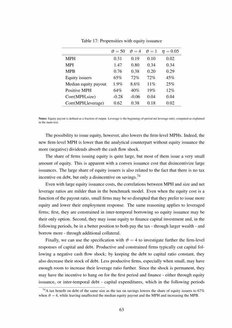
Table 17: Propensities with equity issuance

ϑ = 50 ϑ = 4 ϑ = 1 η = 0.05

MPH 0.31 0.19 0.10 0.02MPI 1.47 0.80 0.34 0.34MPB 0.76 0.38 0.20 0.29Equity issuers 65% 72% 72% 45%Median equity payout 1.9% 8.6% 11% 25%Positive MPH 64% 40% 19% 12%Corr(MPH,size) -0.28 -0.06 0.04 0.04Corr(MPH,leverage) 0.62 0.38 0.18 0.02

Notes: Equity payout is defined as a fraction of output. Leverage is the beginning-of-period net leverage ratio, computed as explainedin the main text.

The possibility to issue equity, however, also lowers the firm-level MPHs. Indeed, thenew firm-level MPH is lower than the analytical counterpart without equity issuance themore (negative) dividends absorb the cash flow shock.

The share of firms issuing equity is quite large, but most of them issue a very smallamount of equity. This is apparent with a convex issuance cost that disincentivize largeissuances. The large share of equity issuers is also related to the fact that there is no taxincentive on debt, but only a disincentive on savings.74

Even with large equity issuance costs, the correlations between MPH and size and netleverage ratios are milder than in the benchmark model. Even when the equity cost is afunction of the payout ratio, small firms may be so disrupted that they prefer to issue moreequity and lower their employment response. The same reasoning applies to leveragedfirms; first, they are constrained in inter-temporal borrowing so equity issuance may betheir only option. Second, they may issue equity to finance capital investment and, in thefollowing periods, be in a better position to both pay the tax - through larger wealth - andborrow more - through additional collateral.

Finally, we can use the specification with ϑ = 4 to investigate further the firm-levelresponses of capital and debt. Productive and constrained firms typically cut capital fol-lowing a negative cash flow shock; by keeping the debt to capital ratio constant, theyalso decrease their stock of debt. Less productive firms, especially when small, may haveenough room to increase their leverage ratio further. Since the shock is permanent, theymay have the incentive to hang on for the first period and finance - either through equityissuance, or inter-temporal debt - capital expenditures, which in the following periods

74A tax benefit on debt of the same size as the tax on savings lowers the share of equity issuers to 67%when ϑ = 4, while leaving unaffected the median equity payout and the MPH and increasing the MPB.

63

expands their wealth and ability to pay the tax. For this reason, 11% of firms display anegative MPI when ϑ = 4, and this share increases to 12% when ϑ = 1.

F Sensitivity of aggregate employment to φ

With a slight abuse of notation, I sort the firms in the economy by their constraint statusand define c as the cutoff below which all firms are constrained. Considering a measure 1of firms, aggregate employment is:

N =

c∫0

nci di+

1∫c

nui di (16)

Then by the means of the Leibniz rule we get:

∂N∂φ

=

c∫0

∂nci

∂φdi+

1∫c

∂nui

∂φdi+

∂c∂φ

[nc(c)−nu(c)] (17)

The economy can be classified in three groups: already constrained firms with a pos-itive MPH, firms becoming constrained due to the change in φ and unconstrained firmswith a zero MPH. For the last group, the derivative of employment with respect to φ is0. For the first group, we can exploit the binding financial constraints. I differentiate thecombined non-negativity of dividends and collateral constraint, when both binding, to get:MPL ∂n

∂φ− ∂n

∂φ− ∂n

∂φ

1φ+ n

φ 2 = 0. This implies:

∂ni

∂φ=

ni

φ 2 MPHi (18)

In order to present more clearly the link between MPH moments and the responseof aggregate employment to a credit tightening, let me now abstract from the effect ofchanges in φ on the share of constrained firms. By doing so, the response of aggregateemployment is approximately given by:

∂N∂φ≈∫ ni

φ 2 MPHidi (19)

This object can be decomposed as follows, in the spirit of the Olley and Pakes (1996)decomposition:

∫ ni

φ 2 MPHidi =1

φ 2

[E(MPH)E(n)+

∫(ni−E(n))(MPHi−E(MPH))di

](20)

64

which can be rewritten as equation 12.

G Aggregate TFP shocks and the MPH

This section works along the lines of 7.2 but for an aggregate TFP shock. Figure 15shows the response of aggregate capital, net debt, labour, output and endogenous TFPto an unanticipated 1% drop in aggregate exogenous TFP, lasting 3 years. Aggregateexogenous TFP is defined as A in the new firm-level production function yt = Az j,tkν

t nαt ;

in steady state, A is 1. Solid lines refer to the economies with the financial frictions,while dashed lines to the economies’ counterparts without. When there are no financialfrictions, the average MPH is 0.

In the blue economy, the average MPH is 0.07, in the red economy is 0.23 while theblack economy depicts the benchmark case with MPH equal to 0.39.

Introducing exogenous exit to an otherwise frictionless economy implies a much strongerresponse of aggregate capital, labour and output. Financial frictions, however, dampen allresponses, and more so the higher the average MPH of the economy. Moreover, the gapopens up as the crisis goes by. At trough, labour has fallen by 15% less in the low-MPH economy than its frictionless counterpart, while the dampening is 10 times larger,at 146%, for the high-MPH economy. Finally, the propagation of the shock, measured interms of years required for output to recover to the pre-crisis episode, is shorter the largerthe MPH of the economy.

65

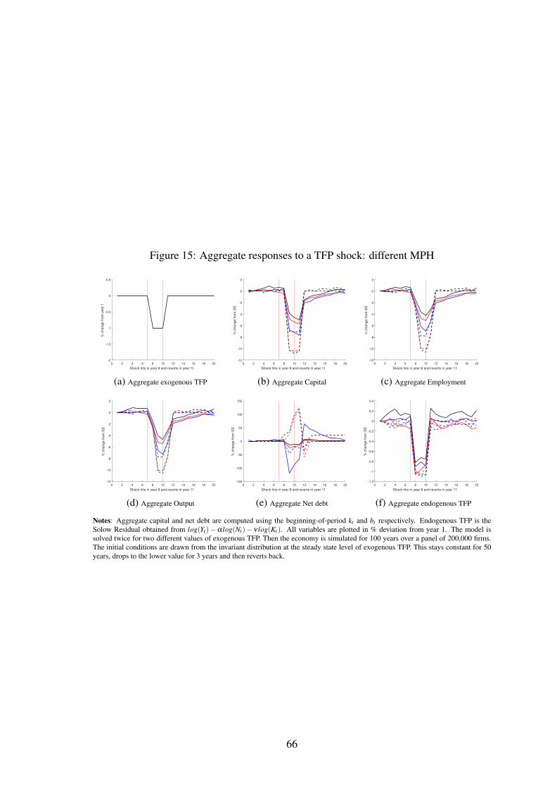
Figure 15: Aggregate responses to a TFP shock: different MPH

0 2 4 6 8 10 12 14 16 18 20

Shock hits in year 8 and reverts in year 11

-2

-1.5

-1

-0.5

0

0.5

% c

ha

ng

e f

rom

ye

ar

1

(a) Aggregate exogenous TFP

0 2 4 6 8 10 12 14 16 18 20

Shock hits in year 8 and reverts in year 11

-12

-10

-8

-6

-4

-2

0

2

% c

ha

ng

e f

rom

SS

(b) Aggregate Capital

0 2 4 6 8 10 12 14 16 18 20

Shock hits in year 8 and reverts in year 11

-12

-10

-8

-6

-4

-2

0

2

% c

ha

ng

e f

rom

SS

(c) Aggregate Employment

0 2 4 6 8 10 12 14 16 18 20

Shock hits in year 8 and reverts in year 11

-12

-10

-8

-6

-4

-2

0

2

% c

ha

ng

e f

rom

SS

(d) Aggregate Output

0 2 4 6 8 10 12 14 16 18 20

Shock hits in year 8 and reverts in year 11

-150

-100

-50

0

50

100

150

% c

ha

ng

e f

rom

SS

(e) Aggregate Net debt

0 2 4 6 8 10 12 14 16 18 20

Shock hits in year 8 and reverts in year 11

-1.2

-1

-0.8

-0.6

-0.4

-0.2

0

0.2

0.4

% c

ha

ng

e f

rom

SS

(f) Aggregate endogenous TFP

Notes: Aggregate capital and net debt are computed using the beginning-of-period kt and bt respectively. Endogenous TFP is theSolow Residual obtained from log(Yt)−αlog(Nt)− ν log(Kt). All variables are plotted in % deviation from year 1. The model issolved twice for two different values of exogenous TFP. Then the economy is simulated for 100 years over a panel of 200,000 firms.The initial conditions are drawn from the invariant distribution at the steady state level of exogenous TFP. This stays constant for 50years, drops to the lower value for 3 years and then reverts back.

66