the market for corporate assets: who engages in mergers...

The Market for Corporate Assets:Who Engages in Mergers and Asset Sales

and Are There Efficiency Gains?

VOJISLAV MAKSIMOVIC and GORDON PHILLIPS*

ABSTRACT

We analyze the market for corporate assets. There is an active market for corpo-rate assets, with close to seven percent of plants changing ownership annuallythrough mergers, acquisitions, and asset sales in peak expansion years. The prob-ability of asset sales and whole-firm transactions is related to firm organizationand ex ante efficiency of buyers and sellers. The timing of sales and the pattern ofefficiency gains suggests that the transactions that occur, especially through assetsales of plants and divisions, tend to improve the allocation of resources and areconsistent with a simple neoclassical model of profit maximizing by firms.

IN THE UNITED STATES there is a large and active market for corporate assets,from individual plants and divisions up to sales of entire corporations. Eachyear over the period 1974 to 1992, an average 3.89 percent of the largemanufacturing plants in the country changed ownership.1 This average maskssubstantial procyclical time variation, so that in expansion years, an aver-age of 6.19 percent of manufacturing plants are involved in mergers andacquisitions and asset sales in each year. While the literature has succeededin providing many insights about the gains and losses in mergers, mergerscomprise only about one half of the total number of assets traded.2 Much lessis known about partial-firm asset sales.3

* Robert H. Smith School of Business, The University of Maryland. This research was sup-ported by NSF Grant #SBR-9709427. We thank Judy Chevalier, John Graham, Peter MacKay,Steven Michael, Harold Mulherin, René Stulz, Michael Vetsuypens, an anonymous referee, andseminar participants at Duke, Illinois, NYU, The National Bureau of Economic Research, Stan-ford, University of Texas at Austin, University of Texas at Dallas, Virginia Tech, and the West-ern Finance Association meetings for helpful comments. We also thank Sang Nguyen andresearchers at the Center for Economic Studies for their comments and help with the data usedin this study. The research was conducted at the Center for Economic Studies, U.S. Bureau ofthe Census, Department of Commerce. The authors alone are responsible for the work and anyerrors or omissions.

1 These statistics are described in detail below.2 For a comprehensive survey see Jensen and Ruback ~1983! and also Ravenscraft and Scherer

~1987!.3 Early studies are Alexander, Benson, and Kampmeyer ~1984!, and Hite, Owers, and Rogers

~1987!. The number of transactions in these studies has been fairly small because the data isdifficult to obtain. Schlingemann, Stulz, and Walkling ~2002! also analyze segment sales.

THE JOURNAL OF FINANCE • VOL. LVI, NO. 6 • DEC. 2001

2019

In this study, we treat mergers, acquisitions, and asset sales as compo-nents of the overall market for firm assets in manufacturing industries.Using detailed plant-level data from the Longitudinal Research Database~LRD! compiled at the Census Bureau, we track sales of individual plantsand benchmark their efficiency against that of other plants in the industry.We ask several questions: Does the market facilitate the reallocation of as-sets to more efficient uses? How big is the market for plants, and each of thesegments ~individual plants, divisions, and entire firms!? What are the fac-tors that drive mergers and asset sales? We also ask whether firm organi-zation affects how firms participate in the market for assets. Does thesubsequent productivity of the transacted plants vary by the buying andselling firms’ organizational characteristics?

An inf luential view in the literature is that major investment and take-over decisions of firms are inf luenced by conf licts of interest between man-agers and the owners of the firm.4 This view suggests that many acquisitionsare undertaken for empire building and managerial entrenchment by man-agers, and that they serve little economic purpose. Morck, Shleifer, and Vishny~1990! provide evidence that the stock market reacts negatively to diversi-fying acquisitions and to acquisitions where the bidder’s managers performpoorly prior to the acquisitions. For asset sales, Jain ~1985! finds that sell-off announcements are greeted positively by the market and that they pro-ceed a period of negative returns for the sellers. Lang, Poulsen, and Stulz~1995! find asset sales follow poor firm-level performance. John and Ofek~1995! find that the remaining assets of the firm improve in performanceafter asset sales that subsequently leave the firm more focused. These stud-ies suggest that transactions either follow inefficient investments by firmsor act to unwind such investments.

An alternative view, modeled in Maksimovic and Phillips ~2002!, positsthat firms grow and purchase assets efficiently across the industries in whichthey operate.5 This model is also consistent with existing evidence.6 The modelmakes specific testable predictions about the timing and the direction ofsales. In our model, firms become focused when their prospects in their mainindustry significantly improve. They may optimally choose to remain un-focused if their prospects in their main industry are not as good as otherfirms that choose to become focused. Firms sell assets in their less produc-tive divisions following positive demand shocks for these divisions.

4 See Jensen ~1986! and Hart and Moore ~1995!.5 The model is based on Lucas ~1978!. Lucas ~1978! and Williamson ~1985! stress the costs of

managing a larger organization.6 We do not have transaction prices or stock price data. Thus, we cannot test whether one

party gains or loses in the stock market as a result of the transaction. The advantage of ourstudy is that we look at actual productivity changes while stock market data includes a re-sponse to the price paid and prior expectations, in addition to the value of any productivitychanges.

2020 The Journal of Finance

The intuition for the Maksimovic and Phillips ~2002! model is simple. Somefirms are more productive and can produce more than other firms from agiven number of plants. Firms adjust in size until the marginal benefit isequal to the marginal cost of production. As output prices increase, the moreproductive firms have a larger gain in value from the assets they control.As a result, they find it optimal to acquire plants from less productive firmsin the industry, even when that entails some increase in the costs of man-agement. By the same token, a positive shock in an industry increases theopportunity cost of operating as an inefficient producer in that industry.Thus, industry shocks alter the value of the assets and create incentives fortransfers to more productive uses. Given the generally positive upward trendin GDP in the U.S. economy during the mid- and late 1980s, the model canexplain the trend towards increased focus over this period.

Empirically we find that the pattern of transactions ~procyclical sales andsubsequent increases in productivity! is consistent with this model. Our em-pirical results show that assets are more likely to be sold ~1! when the econ-omy is undergoing positive demand shocks, ~2! when the assets are lessproductive than their industry benchmarks, ~3! when the selling division isless productive, and ~4! when the selling firm has more productive divisionsin other industries. For mergers and acquisitions, we find evidence that theless productive firms tend to sell at times of industry expansion. Firms aremore likely to be buyers when they are efficient and are more likely to pur-chase additional assets in industries that experience an increase in demand.

Sellers and buyers of individual plants and divisions tend to be large con-glomerates. A firm’s internal organization has a significant effect on theprobability that an asset is sold. Assets are significantly more likely to besold by peripheral divisions than by main divisions of conglomerates. Thesales of main divisions are much rarer events, perhaps because only divi-sions in which the firm has a core competency become main divisions. Forconglomerates, we find that the probability of the whole firm being sold offis negatively correlated with firm size and with firm focus.

Our results show that most transactions in the market for assets result inproductivity gains. The average productivity of the buyer’s and seller’s ex-isting assets is an important determinant of the gain to trade, suggestingthat firms have differing levels of ability to exploit assets, and that theircomparative advantage is in their main industries. The subsequent observedincrease in productivity of the transferred assets is consistent with thesegains offsetting the increased costs to the purchasing firm of managing alarger organization.7 Thus, the market for corporate assets facilitates theredeployment of assets from firms with a lower ability to exploit them tofirms with a higher ability. There is less support for the hypothesis that

7 Thus, the existence of measurable productivity gains following a transfer does not implythat the transfer’s timing is not optimal. A full dynamic model would be necessary to addressthe question of the optimal timing of transfers.

The Market for Corporate Assets 2021

empire building predominantly drives asset purchases. However, becausemeasured gains are negative for a minority of transactions, we cannot rejectthe possibility that some transactions may be motivated by agencyconsiderations.

Our evidence primarily relates to two literatures: the literature on assetsales and the literature on mergers. Our paper views and considers thesetwo types of transactions as part of a larger market for assets. The literatureon sales of plants and divisions is relatively small. Alexander et al. ~1984!,Jain ~1985!, and Hite et al. ~1987! have found a positive stock market re-sponse to asset sales. Lang et al. ~1995! have shown these asset sales followpoor firm-level performance and that the stock-market gains are positive forfirms that pay out the proceeds instead of reinvesting within the firm.8 Johnand Ofek ~1995! show that the remaining assets of the firm improve in per-formance after asset sales that subsequently leave the firm more focused.Maksimovic and Phillips ~1998! show that firms in Chapter 11 tend to selltheir most efficient plants, whereas firms in a control sample tend to selltheir least efficient plants.

Schlingemann, Stulz, and Walkling ~2002! ~SSW! examine sales of divi-sions. They compare firms that report the sale of one or more whole seg-ments with a control sample of firms which do not divest. Working withaccounting data, they predict how firms choose which segments to divest.SSW’s principal finding is that the liquidity of the market for assets playsan important role in determining which asset is divested. The probabilitythat a segment is divested is higher if the asset is in an industry with aliquid market for assets and if it performs poorly. The divested segments areon average smaller than segments that are retained.

There is a large literature on the gains from mergers that has examinedthe gains to the bidders and targets in the stock market. Lang, Stulz, andWalkling ~1991! show that the total stock market gains in tender offers arehighest when the bidder has a high Tobin’s q and the target has a low q. Thisis consistent with the notion that gains are highest when well-managed firmstake over badly managed firms. Less is known about the gains in partialfirm sales. Several studies have examined the cash f low performance of firmsbefore and after mergers. Matsusaka ~1993! examines the ex ante financialperformance of firms before they merge and Ravenscraft and Scherer ~1987!examine the ex post financial performance of mergers using FTC line-of-business data. Other studies that have documented performance changesfollowing mergers using the LRD include Lichtenberg and Siegel ~1992! andMcGuckin and Nguyen ~1995, 1999!. McGuckin and Nguyen ~1999! show

8 The advantage over using stock market data and event studies is that a stock marketresponse ref lects the price paid relative to anticipated gains. Gains in productivity can stilloccur if the excess stock market return equals zero if the seller captures the gains. Similarly acombined positive stock market response ~for buyers and sellers! may ref lect information beingrevealed about the assets’ value in the future and may not represent any real productivitygains.


that whether a firm is multiplant or single plant affects observed produc-tivity gains. Kaplan and Weisbach ~1992! track firms after they merge andfind that divestiture rates by purchasers of unrelated firms are higher thanpurchasers of related firms. Even the firms that were broken up, however,show positive combined stock market responses ~buyer and seller! at thetime of the acquisition and do not show declines in operating performancebefore they are broken up. Our theory predicts that firms will buy assetsoutside of their main areas of expertise during recessions and sell unrelatedassets to firms expanding their core business units during booms. Fluck andLynch ~1999! also predict that conglomerate firms maximizing shareholdervalue will buy firms outside of their primary area of expertise duringrecessions.

Following Jensen ~1986!, several authors argue that firm investment andgrowth can be explained by managers’ tendency to overinvest in projectsthat yield private gains. Using data on bidding firms, Lang et al. ~1991!show that the shareholders do not benefit if acquisitions are made using freecash f lows. Scharfstein ~1997! and Rajan, Servaes, and Zingales ~2000! ar-gue that investment distortions are endemic within conglomerates. A similarlogic might suggest that firms acquire plants and divisions that they cannotrun efficiently. By contrast, our view of acquisitions is based on Maksimovicand Phillips ~2002!, who show that the growth by conglomerates’ divisions isconsistent with a simple profit-maximizing model with scarce managerial ororganizational ability. Graham, Lemmon, and Wolf ~2002! show that con-glomerate firms purchase firms that have lower Tobin’s q than the firmsthat remain single-segment firms. Chevalier ~1999! also shows that conglom-erate firms purchase firms that have a different sensitivity of cash f low toinvestment than firms that conglomerates choose not to purchase. Theseresults are consistent with our model and evidence that conglomerate firms,given productivity differences, make selective acquisitions of certain types offirms.9

Two recent studies by Mitchell and Mulherin ~1996! and Andrade andStafford ~1999! show that industry characteristics such as technologicalchanges and capacity utilization are strongly associated with the incidenceof mergers, takeovers, and investment. We are able to exploit plant-leveldata to obtain a more detailed picture of intraindustry firm-level determi-nants of asset transactions. Our evidence suggests that firm organizationand efficiency drives most of the intraindustry trades.

The remainder of this paper is organized as follows. We discuss our ana-lytical framework of analysis in Section I. The data is discussed in Sec-tion II. Section III presents the descriptive statistics of the market for assets.The firm’s decisions to buy and sell and the gains from the transaction areanalyzed in Sections IV and V, respectively. Section VI concludes.

9 The evidence in Maksimovic and Phillips ~2002! shows that conglomerates grow their moreproductive segments faster.


I. Framework for Analyzing Trades in Assets

The hypotheses that we examine are motivated by a neo-classical model offirm organization across multiple markets, advanced by Maksimovic andPhillips ~2002!. Firms sell some or all their assets when there is an expectedgain in productivity if the assets are operated by another firm. These tradesoccur because firms differ in organizational ability and these differencesdetermine their productivity in different industries. The model shows how aprofit-maximizing firm chooses the quantity of capacity to employ in eachindustry and how demand shocks in one industry affect capacity decisions inother industries. It provides predictions on how firm organization affectswho trades assets, and the magnitude of the gains from such activity. Thesepredictions differ from the predictions of models that assume that firmsacquire assets outside their main industry because managers engage in em-pire building behavior. Thus, the predictions of the model can be used to testthe hypothesis that the trade in assets by multiindustry firms allocates as-sets to more productive uses. This section describes the model and sets outthe hypotheses motivated by the model.

Consider first the market for assets when firms maximize profits andfinancial market imperfections are not material. Following Lucas ~1978!,Maksimovic and Phillips ~2002! argue that management teams of firms orfirm organizations differ in their ability to operate plants efficiently.10 Man-agement teams of all abilities find it more difficult to manage a large firmthan a small firm. Thus, a high quality management team may operate amarginal plant in a large firm only as efficiently as a low quality manage-ment team operates a marginal plant in a small firm. Firm size and thescope of a firm’s operations adjust until the profit from operating the mar-ginal plant is equalized across all firms in the industry. As industry condi-tions change, a firm’s comparative advantage in operating plants also changes.As a result, there are gains to trading assets, and trade occurs until theprofit from operating the marginal plant is again equalized. In the equilib-rium, firms with more skilled managers or organizations still have a higheraverage productivity than firms managed by less skilled managers.

The model focuses on how changes in industry demand affect the marginalvalue of plant production in single-segment and in multisegment firms, andthus the direction and the gains to trade in plants. As demand increases,output prices also increase, and the ability to produce more output per unitinput becomes relatively more valuable. The increased value of output isnow greater than the increased cost of operating the firm at a larger size.More productive firms can sell the output at a price that is high enough tocompensate for the diseconomies of operating at a larger size. This raises the

10 More generally, their model can be reinterpreted as positing the existence of a fixed firm-specific factor of production that induces diminishing returns to scale. Following Lucas ~1978!,they identify this factor with managerial, or more generally, organizational ability.


price of capacity in the market for physical assets and less productive man-agers will find it more advantageous to sell their plants to more productivemanagers instead of producing output themselves.

Thus the model predicts that assets f low from more productive to lessproductive firms when demand increases.11 The divisions with more skilledmanagement teams thus gain in size relative to divisions managed by lessskilled managers in the same industry. The volume of sales is higher whenthe technology in the industry is such that productivity does not decreasesteeply as a firm acquires more capacity in the industry. The magnitude oftransactions in response to such demand shocks depends, in part, on whetheror not there are significant diseconomies of scale.

When demand falls, the costs of managing a large firm outweigh the ben-efits of high productivity and at the margin firms may shed assets. How-ever, if the overall trend in the economy exhibits positive growth, we wouldexpect the magnitude of this f low to be lower empirically. Firms would ex-pect such transactions to be reversed subsequently when economic growthresumes. In addition, the existence of transaction costs would reduce theincentive to engage in such transactions, as the opportunity cost of an assetbeing operated outside its best use is lower in a recession. Under these con-ditions, the incentives to engage in transactions will be larger after positiveindustry shocks, giving rise to more transactions when demand increases.

To summarize, the profit-maximizing model suggests tests of the followingpredictions.

HYPOTHESIS 1: Sales of assets are more likely to occur when the industry re-ceives a positive demand shock. The higher (lower) the productivity of a di-vision (or a single-segment firm) the higher the probability that it buys (sells).

Trade-offs between managerial ability and size also hold within multiseg-ment firms. A firm grows its segments until the value of a marginal invest-ment is equalized across industries in which it operates. Thus, the growthand efficiency of a segment may affect a firm’s decision to buy or sell plantsin another segment. The model predicts that a firm reduces its capacity inan industry by selling assets when the value of these assets to another firmis higher. The opportunity cost may be high either because other firms inthe industry can better use the assets, or because the selling firm has betterprospects in other industries. Thus, a multisegment firm sells plants in asegment when its other segments are growing fast and it is an efficientproducer in these other segments. It may also sell a segment when the seg-ment is not an efficient producer, but the industry is doing well and theplant is relatively more valuable to other, more efficient, producers. Thesepredictions are summarized in the following hypothesis.

11 The model allows buying of new capacity from an external market with an upward slopingsupply curve. An upward sloping supply curve can be justified given adjustment costs for newcapacity, or through time-to-build, or given increasing costs of needed inputs to build new ca-pacity. Firms may also scrap assets if the demand in the industry is sufficiently low.


HYPOTHESIS 2: Asset trades in multisegment firms follow a specific pattern:There is an increased probability that a segment is sold (purchased), when(1) the firm has lower (higher) productivity in an industry and this industryreceives a positive demand shock, and (2) the firm’s other segments havehigher (lower) relative productivity and these other industries receive positivedemand shocks.

The asset purchase decision works similarly to the sale decision. Multi-segment firms may purchase plants in an industry if their other segmentsare less productive producers in industries that receive a positive demandshock. In that case, these less productive segments optimally sell out tomore productive producers in their respective industries, and the firm ex-pands faster in its remaining segments. Firms may also purchase plants inan industry when their prospects elsewhere diminish. This occurs if they aremore productive producers in other industries and these industries suffernegative demand shocks.

This prediction may also be used to distinguish the neoclassical modelfrom several hypotheses about the acquisition decisions of multisegment firmswhen managers act opportunistically or when there are material financialmarket imperfections. Lamont ~1997!, for example, suggests that firms wouldbe more likely to invest outside their main divisions when their main divi-sion receives a positive demand shock. Thus, if the main division of firms ismore efficient than peripherals, this prediction on the effect of demand shockson the purchase and sale decisions in other industries is opposite to that ofour model.

Jensen’s ~1986! free cash f low theory suggests that when firms have ex-cess cash f low, they tend to use it to acquire additional assets that theycannot operate efficiently. More recently Rajan et al. ~2000! and Scharfsteinand Stein ~2000! have also argued that the organizational structure of con-glomerates makes them likely to waste assets. Although we cannot identifythe dissipation of shareholder wealth from managers overpaying for acqui-sitions or the appropriation of cash f lows from assets, our empirical testswill detect the extent to which the dissipation of free cash f lows in multi-segment firms leads to acquisition patterns that differ from those predictedby efficient allocation across industries.

These predictions regarding the f low of assets between firms have impli-cations for the analysis of firm organization and restructuring. Profit-maximizing firms grow more in industries in which they have a comparativeadvantage. Thus, on average, the larger divisions of multisegment firms arepredicted to have a higher mean productivity than smaller, peripheral divi-sions.12 As a result, in the long run, main divisions are more likely to bebuyers and peripheral divisions are more likely to be sellers. For the same

12 Maksimovic and Phillips ~2002! examine this prediction and show it to be consistent withsegment-level data constructed from underlying plant-level census data.


reason the expected gain in productivity is higher when the plant is sold bya peripheral division and purchased by a buyer’s main division than if thepurchase is of a plant in a buyer’s peripheral division.

The differences in productivity between main and peripheral units of thesame firm are also likely to create an association between organizationalstructure and trades following a demand shock. When the main division ofa multisegment firm receives a positive demand shock, the firm will sellcapacity in the peripheral divisions. When the main unit receives a negativedemand shock, the firm will acquire assets in peripheral units.13 We sum-marize these predictions in the following hypothesis.

HYPOTHESIS 3: Multisegment firms increase their focus through acquisitionswhen demand is high in their main industries, and decrease their focuswhen demand is low. The probability that an asset is sold and the expectedgain from the sale are higher for assets operated by peripheral divisions offirms.

Our model does not make a distinct prediction for transactions involvingthe whole firm—such as mergers—and transactions involving only some plantsor divisions. In fact, we expect the model to predict mergers less well thanpartial firm transactions: Mergers or acquisitions of multidivisional firmsmay involve the transfer of some divisions that do not fit under new own-ership and that would not have occurred in isolation.14

II. Data

We use data from the Longitudinal Research Database ~LRD!, maintainedby the Center for Economic Studies at the Bureau of the Census.15 The LRDdatabase contains detailed plant-level data for manufacturing plants ~SICcodes 2000–3999! on the value of shipments produced by each plant, invest-ments broken down by equipment and buildings, and the number of employ-ees. The LRD tracks approximately 50,000 manufacturing plants every yearin the Annual Survey of Manufactures ~ASM!. This database is only a surveyfor smaller plants. The ASM covers all plants with more than 250 employ-ees. In addition, it also includes smaller plants that are randomly selectedevery fifth year to complete a rotating five-year panel. Once selected, plants

13 We would also expect to see similar effects on other divisions when peripheral units re-ceive demand shocks. However, because peripheral units are smaller than main units, theseeffects are less likely to be detectable.

14 Another model that has implications for the timing of asset sales is Shleifer and Vishny~1992!. Shleifer and Vishny stress the importance of asset sales that occur by firms with highdebt when industries become temporarily distressed. We do not examine the predictions of thismodel in this paper given that this database does not have financial structure variables.

15 For a more detailed description of the Longitudinal Research Database ~LRD! see McGuckinand Pascoe ~1988!.


are required by U.S. law to answer the questions. Many data items used~e.g., the number of employees, employee compensation, total value of ship-ments! also represent items that are also reported to the IRS, increasing theaccuracy of the data.

There are several advantages to this database. First, it covers both publicand private firms in manufacturing industries. Second, coverage is at theplant level, and output is assigned by plants at the four-digit SIC code level.Thus, firms that produce under multiple SIC codes are not assigned to justone industry. Third, plant-level coverage means that we can track plantseven as they change owners. In addition to a plant-level identifier, the data-base contains a code that identifies which assets change ownership. Thesetwo features are key to our study, as they allow us to identify assets thathave changed hands from year to year. Thus, plants have to be part of anASM panel for the plants to remain in our study.

We confine our analysis to the period 1974 through 1992. We use 1974 asthe starting year of our analysis because it is the first year of a five-yearpanel; 1992 is the last year of data available to us. We aggregate plants intofirm-level business segments at the three-digit SIC code level and excludesegments that are less than $1 million in real value of shipments in 1982dollars. Our regressions contain observations beginning in 1979 given weuse five years of lagged data in order to calculate productivity for each plantin each year.

III. The Basic Facts

Before preceding to test the hypotheses from the prior section, we firstdescribe the data and present some basic facts about the market for assets.

A. The Number and Types of Transactions

We classify firms as single segment or multiple segment based on three-digit SIC codes. If a firm produces 97.5 percent of its sales or higher in onethree-digit SIC code, we classify that firm as a single-segment firm andexclude the small peripheral segment. We classify all other firms as multiple-segment firms. For these firms, we also classify each segment as either amain segment or a peripheral segment. Main segments are segments whosereal value of shipments ~in 1982 dollars! is at least 25 percent of the firm’stotal shipments.

We classify transactions into three types: single-plant transactions by single-plant firms, multiplant transactions broken into full divisions and partialdivisions ~at the three-digit SIC code level!, and full-firm transactions. Webreak transactions into these three categories as it seems plausible thattransactions in which a single plant changes hands between multiplant firmsin the same industry are marginal investment transactions that have theleast implications for both future investment policy and corporate control.


Transactions in which a division is sold have greater implications for man-agerial control. Finally whole-firm transactions ~mergers and acquisitions!include the purchase of a whole multisegment firm, and thus buyers mayobtain extra assets outside of their area of expertise that they would nototherwise acquire. Gains may thus differ across transaction types.

Table I presents summary statistics for asset reallocations in our data setbetween 1974 and 1992. We break out the transactions into whole-firm dis-positions ~mergers and takeovers! and sales of assets by firms that remainin existence.16

Table I shows that from 1974 to 1992, the total number of plants reallo-cated in mergers and takeovers was approximately equal to the total num-ber of plants reallocated in sales by ongoing firms. On average, 1.95 percentof plants are reallocated annually through takeovers and mergers, whereas0.95 percent and 0.99 percent are reallocated through sales of entire andpartial divisions, respectively. In each case, the plants reallocated tend to bebelow average in size ~real value of shipments! for their industry. More plantsthan not are sold to buyers whose major focus is producing in the sameindustry, defined at the three-digit SIC code level.17 The proportion of sameindustry buyers is lowest for whole-firm dispositions, and highest for partial-division sales. Table I also shows that more transactions occur in industriesthat are in expansion than in recession.

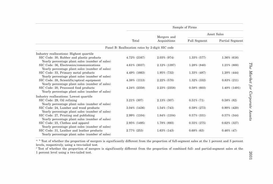
Table I also shows the two-digit SIC code industries with the highest andlowest rates of reallocations in our sample. The highest annual rate is 4.72percent, for Rubber and Plastics, followed by Electronics, Primary Metalproducts, Optical Equipment, and Processed Food Products. The lowest an-nual reallocation rate is 2.77 percent, for Leather and Leather Products,followed by Clothes and Apparel, Printing and Publishing, Lumber and Woodproducts, and Oil Refining. Comparing the types of transactions across in-dustries, it is evident that the rates of partial- and full-division sales inparticular differ considerably within these industries. Thus, for example,the full-division sales rates for Rubber and Plastics and Leather and LeatherProducts are 1.33 percent and 0.68 percent, respectively. The correspondingrates for partial-division sales are 1.36 percent and 0.46 percent, respectively.

B. Who Are the Buyers and Sellers?

Table II shows the characteristics of the firms that sell and acquire assets,by transaction category. In the table, we also break out mergers and acqui-sitions into those that involve sellers with just one plant, sellers in just oneindustry, and sellers who operate in more than one industry. In all cases, thecharacteristics are measured in the year prior to the transaction. The ac-quiring firm in the case of partial and full divisional sales is the buying

16 Thus, a firm that sells its only division is classified as a merger.17 More precisely, buyers for whom that industry is one of the top two industries in which

they operate, and who produce at least 25 percent of their output in that industry.


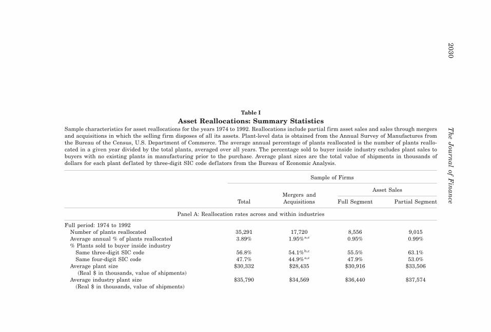
Table I

Asset Reallocations: Summary StatisticsSample characteristics for asset reallocations for the years 1974 to 1992. Reallocations include partial firm asset sales and sales through mergersand acquisitions in which the selling firm disposes of all its assets. Plant-level data is obtained from the Annual Survey of Manufactures fromthe Bureau of the Census, U.S. Department of Commerce. The average annual percentage of plants reallocated is the number of plants reallo-cated in a given year divided by the total plants, averaged over all years. The percentage sold to buyer inside industry excludes plant sales tobuyers with no existing plants in manufacturing prior to the purchase. Average plant sizes are the total value of shipments in thousands ofdollars for each plant def lated by three-digit SIC code def lators from the Bureau of Economic Analysis.

Sample of Firms

Asset Sales

TotalMergers andAcquisitions Full Segment Partial Segment

Panel A: Reallocation rates across and within industries

Full period: 1974 to 1992Number of plants reallocated 35,291 17,720 8,556 9,015Average annual % of plants reallocated 3.89% 1.95%a,c 0.95% 0.99%% Plants sold to buyer inside industry

Same three-digit SIC code 56.8% 54.1%b,c 55.5% 63.1%Same four-digit SIC code 47.7% 44.9%a,c 47.9% 53.0%

Average plant size~Real $ in thousands, value of shipments!

$30,332 $28,435 $30,916 $33,506

Average industry plant size $35,790 $34,569 $36,440 $37,574~Real $ in thousands, value of shipments!

2030T

he

Jou

rnal

ofF

inan

ce

Sample of Firms

Asset Sales

TotalMergers andAcquisitions Full Segment Partial Segment

Panel B: Reallocation rates by 2-digit SIC code

Industry reallocations: Highest quartileSIC Code: 30, Rubber and plastic products

Yearly percentage plant sales ~number of sales!4.72% ~2167! 2.03% ~974! 1.33% ~577! 1.36% ~616!

SIC Code: 36, Electronics0communicationsYearly percentage plant sales ~number of sales!

4.61% ~3037! 2.12% ~1397! 1.28% ~840! 1.21% ~800!

SIC Code: 33, Primary metal productsYearly percentage plant sales ~number of sales!

4.49% ~1663! 1.95% ~732! 1.33% ~487! 1.20% ~444!

SIC Code: 38, Scientific0optical equipmentYearly percentage plant sales ~number of sales!

4.38% ~1113! 2.22% ~570! 1.32% ~332! 0.83% ~211!

SIC Code: 20, Processed food productsYearly percentage plant sales ~number of sales!

4.24% ~2358! 2.23% ~2358! 0.58% ~603! 1.40% ~1491!

Industry reallocations: Lowest quartileSIC Code: 29, Oil refining

Yearly percentage plant sales ~number of sales!3.21% ~307! 2.13% ~307! 0.51% ~71! 0.58% ~82!

SIC Code: 24, Lumber and wood productsYearly percentage plant sales ~number of sales!

3.04% ~1436! 1.54% ~743! 0.59% ~273! 0.90% ~420!

SIC Code: 27, Printing and publishingYearly percentage plant sales ~number of sales!

2.99% ~1104! 1.84% ~1104! 0.57% ~331! 0.57% ~344!

SIC Code: 23, Clothes and apparelYearly percentage plant sales ~number of sales!

2.95% ~1495! 1.78% ~893! 0.55% ~275! 0.62% ~327!

SIC Code: 31, Leather and leather productsYearly percentage plant sales ~number of sales!

2.77% ~253! 1.63% ~143! 0.68% ~63! 0.46% ~47!

a, b Test of whether the proportion of mergers is significantly different from the proportion of full-segment sales at the 1 percent and 5 percentlevels, respectively, using a two-tailed test.c Test of whether the proportion of mergers is significantly different from the proportion of combined full- and partial-segment sales at the1 percent level using a two-tailed test.

Th

eM

arketfor

Corporate

Assets

2031

Table II

Asset reallocations: Summary StatisticsSample characteristics for asset reallocations for the years 1974 to 1992. Reallocations include partial firm asset sales and sales through takeoversand mergers in which the selling firm disposes of all its assets. Plant-level data is obtained from the Annual Survey of Manufactures from theBureau of the Census, U.S. Department of Commerce. Recession ~expansion! years are the three years classified as having the largest decline~expansion! in the aggregate real value of industrial production. Industry capacity utilization quartiles are yearly quartiles based on the ratesreported by the Department of the Census. Long-run industry growth0decline quartiles are calculated using growth rates for aggregate industryshipments over a 15-year period, with beginning and ending periods representing three-year averages for 1974 to 1976 and 1990 to 1992.

Sample of Firms

Asset Sales

TotalMergers and

Takeovers Full Division Partial Division

Transactions by aggregate economy conditionsRecession years ~1981, 1982, 1991!

Average % reallocated ~total number! 3.57% ~5,148! 2.16% ~3,112! 0.70% ~1,003! 0.72% ~1,033!Expansion years ~1986, 1987, 1988!

Average % reallocated ~total number! 6.19% ~8,989! 2.69% ~3,904! 1.73% ~2,509! 1.77% ~2,576!Indeterminate Years 3.21% 1.73% 0.70% 0.78%

Transactions by industry capacity utilizationLow industry capacity utilization ~bottom quartile!

Average % reallocated ~total number! 3.86% ~8,618! 1.90% ~4,244! 0.99% ~2,210! 0.97% ~2,164!High industry capacity utilization ~top quartile!

Average % reallocated ~total number! 3.69% ~8,413! 1.92% ~4,375! 0.87% ~1,977! 0.90% ~2,061!

Transactions by long-run industry growth0declineQuartile 1: Declining industry growth

Average % reallocated ~total number! 4.01% ~6,290! 1.95% ~3,058! 1.09% ~1,707! 0.97% ~1,525!Quartile 2

Average % reallocated ~total number! 3.86% ~5,250! 1.96% ~2,666! 1.05% ~1,425! 0.85% ~1,160!Quartile 3

Average % reallocated ~total number! 3.52% ~10,008! 1.80% ~5,131! 0.88% ~2,505! 0.83% ~2,372!Quartile 4: High industry growth

Average % reallocated ~total number! 4.03% ~15,746! 2.01% ~7,870! 0.87% ~3,405! 1.14% ~4,471!

2032T

he

Jou

rnal

ofF

inan

ce

firm. In the case of mergers and acquisitions, these are the surviving firms.For mergers we also report the characteristics of buyers who operate inmultiple three-digit SIC code industries.

Firms that sell full and partial divisions tend to be quite large ~averagerevenues of $1.328 and $1.849 billion! and operate in an average of approx-imately eight three-digit industries. Sellers of partial divisions tend to op-erate a greater number of plants ~an average of 31.48 in contrast to anaverage of 23.72 plants operated by sellers of entire divisions!. Only approx-imately a quarter of the plants sold in the sales of entire divisions belong toone of the seller’s main divisions, whereas approximately half of plants soldin partial division sales belong to one of the seller’s main divisions.

Buyers of entire divisions are of similar size and operate a similar numberof plants as the sellers, whereas the buyers of partial divisions are on aver-age about two thirds as large as the sellers. Buyers in both categories tendto be slightly more focused than the sellers, operating in an average of ap-proximately six three-digit SIC code industries. The buyers’ main divisionsacquired 53.8 percent and 63.1 percent of the plants purchased in entire andpartial-division transactions, respectively. Thus, the market for asset salesis one in which both the buyers and sellers are conglomerate firms. Thesellers sell peripheral divisions and marginal plants to the main divisions ofthe buyers. Although the buyers are somewhat smaller and more focusedthan the sellers, the differences between them are not large.

In contrast, the average seller in a merger operates 1.78 plants and hassales of $51 million. Approximately 80 percent of all full-firm sales ~mergersand purchases! involve the sale of small, one-plant firms. About 10 percentof all mergers involve multiplant single-industry firms ~average number ofplants, 5.15! and approximately 10 percent involve multiple-industry firms.Even in this last category, the sellers have an average of only 7 plants, havesales of $239 million, and operate in an average of approximately three three-digit SIC code industries. Buyers of whole firms are larger than the sellers.On average, they operate 16.64 plants, produce in 4.66 three-digit SIC codeindustries, and have annual sales of $856 million. About a half of the ac-quired plants are operated by the buying firms’ main divisions.

To summarize, we find several differences between the buyers in partialfirm dispositions and mergers. On average, buyers of full or partial divisionstend to be larger than buyers in mergers, they operate more plants, and tendto operate in a larger number of industries. These differences arise becausea larger proportion of buyers in mergers are single-industry firms. The sub-set of buyers in mergers who operate in multiple industries are slightly big-ger in size and in the number of industries in which they operate.

C. Aggregate and Industry Demand and Asset Reallocations

We compare asset reallocations during economic expansions and reces-sions. We classify years as recession or expansion years by using aggregateand aggregate-detrended industrial production. Detrended industrial pro-


duction is defined as the actual less predicted industrial production, wherewe calculate predicted industrial production from a regression of industrialproduction on a yearly time trend. Recession years are years in which bothreal and detrended industrial production decline relative to the previousyear. We classify years as expansion years when both real and detrendedindustrial production increase relative to the previous year.

This procedure gives us results similar to the NBER recession dating pro-cedure, which the NBER does quarterly. This procedure also allows us toclassify a year such as 1980, which, according to the NBER, had a recessionof less than six months. Using this procedure, we classify 1981, 1982, and1991 as recession years. For comparability, we also take the top three ex-pansion years—1986 through 1988. ~Other expansion years were 1976 through1978 and 1984 through 1985.! Given that actual and detrended industrialproduction did not move in the same direction, 1979, 1980, 1983, 1989, and1992 are indeterminate years.

Table III shows that more assets are reallocated in expansions. The ratesof reallocations during expansion years ~the three years with the highestincreases in the aggregate real value of industries production! and recessionyears ~the three years with the largest decline in the aggregate real value ofindustries production! are 6.20 percent and 3.57 percent, respectively. Therates of full- and partial-division sales, in particular, are much higher inexpansions ~1.73 percent and 1.78 percent, respectively!, than in recessionyears ~0.70 percent and 0.72 percent, respectively!. The reallocations ratedue to mergers is somewhat higher in expansions than in recessions ~2.69 per-cent compared to 2.16 percent!. By contrast, the total reallocation rate in theremaining indeterminate years is 3.21 percent, the reallocation rate due tomergers is a low 1.73 percent, whereas the partial- and full-division salesrates are 0.78 percent and 0.70 percent, respectively. Thus, the partial- andfull-division sales are sharply higher in expansion years.

We find that the number of transactions is sharply higher in expansions.The fact that transactions are lower in recessions is consistent with theoverall positive growth trend in the economy causing firms to expect to needmore capacity in the future, when growth resumes. In addition, transactionsin recessions may result in gains that are less likely to offset transactionscosts because the opportunity cost of an asset being operated outside its bestuse is lower in a recession.

We next explore differences in capacity utilization on the rate of transac-tions. We use industry-level capacity utilization data from the Bureau of theCensus. For each year we use capacity utilization to classify into quartilesall the three-digit SIC industries. We report the average rate of transactionsover the sample period for the top and bottom quartile. As Table II shows,the rates of reallocation do not differ materially across capacity utilizationquartiles.

We also report the rates of reallocations by long-run industry growth. AsTable III shows, more reallocations take place in the fastest growingindustries—15,746 in the fastest growing quartile compared to 6,290 in the


Table III

Buyer and Seller CharacteristicsSample characteristics of purchasing firms prior to asset purchases for the years 1974 to 1992. Data is aggregated to firm-level from individualmanufacturing plants. Plant-level data is from the Annual Survey of Manufactures from the Bureau of the Census, U.S. Department of Com-merce. Buyers without any prior manufacturing plants ~foreign buyers, outside manufacturing buyers! are excluded as prepurchase character-istics can not be calculated. Average buyer and seller size is the average value of total shipments def lated by industry price def lators from theBureau of Economic Analysis. 1992 was the last year available at the time the study was conducted.

Sample of Firms

Asset Sales Mergers and Takovers

FullDivision

PartialDivision

Firms withPlants 5 1

Firms withPlants . 1

Multiple Industry Firms~Three-digit SIC Code!

Seller characteristics prior to saleFull period: 1974 to 1992

Number of selling firms 3,774 4,205 9,480 2,204 1,224Average number of plants 23.72 31.48 1.00 5.15 7.0Average seller size ~millions $! 1,328 1,849 22 176 239Average number of three-digit industries 7.56 7.77 1.00 2.21 3.17Average number of four-digit industries 9.58 10.56 1.00 2.53 3.61% of plants sold by seller in its primary line of business

Seller’s primary three-digit line~s!* 28.2% 50.8% 100.0% 70.6% 62.2%Seller’s primary four-digit line~s!* 25.6% 36.3% 100.0% 61.6% 54.9%

Buyer characteristics prior to purchaseFull period: 1974 to 1992

Number of buyers 2,267 2,755 1,648 4,530 3,627Average number of plants 23.50 23.38 1.00 22.33 26.80Average buyer size ~millions $! 1,307 1,357 27.9 1,157 1,410Average number of three-digit industries 6.24 5.75 1.00 6.00 7.24Average number of four-digit industries 8.21 7.58 1.00 7.87 9.51% of plants bought that are in buyer’s home industry

At the three-digit SIC code 53.8% 63.1% 59.1% 30.8% 26.3%At the four-digit SIC code 47.9% 55.2% 49.9% 21.0% 17.4%

* If the seller ~buyer! produces in multiple industries, the seller’s ~buyer’s! home industries are those industries that have at least 20 percent of the firm’s sales.

Th

eM

arketfor

Corporate

Assets

2035

slowest growing quartile of industries. However, the overall rate of transac-tions is similar at approximately four percent. There is some limited evidencethat industries which have more moderate growth rates have a somewhatlower rate of transactions, but the effect, if it exists, is relatively small.

We also subclassify the reallocations into those that occurred in years inwhich the industry ~at the three-digit SIC level! was in expansion, and thosethat occurred in years in which the industry was in recession. For an indus-try to be classified as being in expansion, its real production in that year hasto increase and its real level of output has to exceed its long-term trendlevel. For an industry to be classified as being in recession, the industry’sreal output has to decline in that year and the real level of output has to bebelow the long-term trend level.

Table III suggests that the average rate of reallocations, and in particularthe rate of partial firm sales, is higher in periods of macroeconomic expan-sion. There is less evidence that differences in industry conditions have amaterial effect.

A similar pattern emerges when the time series of sales is plotted. Fig-ure 1 shows both the annual rate of reallocations and detrended aggregateindustrial production. Detrended industrial production is calculated as de-scribed earlier.

Figure 1. Left-hand scale is the total percentage of plants changing ownership byyear. Right-hand scale is aggregate real industrial production detrended.


Figure 1 shows that, consistent with Table II, the annual percentage ofplants that transferred ownership is high in expansions. It is highest in1986 and in 1987, when nearly seven percent of the plants change ownership~adding up mergers and full- and partial-firm asset sales!. The proportion oftransactions that occur in industries that are in expansion also varies con-siderably, and is procyclical. In 1987 and 1988, when few industries are inrecession, the number of plants transacted in these industries clearly declines.

However, when we plot the time series of the proportion of plants trans-acted in industries that were in recession and expansion in Figure 2, we findthat the proportions are very similar. The reason for this result is that fewindustries are in recession when the overall economy is in expansion. Thosethat are in recession have a similar proportion of plants transacted. Thus,time series variation in the overall rate of asset reallocations is driven byeconomy-wide factors.

We next examine the time series variation in the percentage of plantsbroken down by mergers and acquisitions, division sales and partial-divisionsales. Figure 3 breaks the transactions into these categories. In particular,mergers are strongly procyclical, rising in the years before the 1982 reces-sion to over three percent of plants, before falling to one percent of plants in1984. The rate of mergers and acquisitions increased again to almost fourpercent of plants by 1987. Partial-firm asset sales vary less year by year;however they still hit a peak of over four percent ~combining full and partialsegment sales! in 1987.

Figure 2. Change of ownership by type of industry. Expansion ~recession! industries arethe industries in which real and detrended value of shipments at the industry level increase~decline!.


The summary statistics suggest that the rate of asset sales, and in par-ticular of full- and partial-divisions sales, is affected by economy-wide fac-tors. There is less evidence that the average rate of transactions is affectedby industry factors, such as capacity utilization and long-term growth. Wenext explore how within-industry and within-firm characteristics affect whichfirms sell plants and what plants firms choose to sell.

IV. The Probability of an Asset Sale

A. How Sales Vary with Firm Organization

In Figure 4, we show how the proportion of assets sold by division rank,where rank equals one for the largest segment by real value of shipments.

For firms with a given number of segments, as the segment rank of aparticular segment increases, the proportion of its assets sold also increasessharply. The plants in the largest segment of a firm are the least likely to besold. For example, the proportion of largest segment plants sold is less thanone percent for firms with seven or more segments, whereas the proportionof plants that these firms sell in their smallest segments rises to three andfour percent. Schlingemann et al. ~2002! find using accounting data on whole

Figure 3. Percentage of plants reallocated through mergers, full-segment sales, andpartial-segment sales by year.


segments that a firm is more likely to sell small rather than large segments.Maksimovic and Phillips ~2002! find that there is an inverse relation be-tween the rank of a segment and its efficiency, and that the equally rankedsegments of larger firms tend to be more efficient than those of smaller firms.Thus, Figure 4 accords well with the hypothesis that firms are more likely tosell their least efficient plants and also that, holding segment ranks constantacross firms, the rate of plant sales is lower for more efficient segments.

There also exists an inverse relation between the number of segments afirm possesses and the probability that it will be acquired. Three percent ofsingle-segment firms are bought out or merged, whereas only 1.5 percent offirms with six and seven segments are merged.

B. Measurement of Productivity and Demand in Business Segments

To analyze the relation between demand and firms’productivity on asset sales,we need measures of both these variables. We discuss our measures next.

B.1. Productivity of Business Segments

We calculate productivity for all firm segments at the plant level. Ourprimary measure of performance is total factor productivity ~TFP!. TFP takesthe actual amount of output produced for a given amount of inputs and

Figure 4. Percentage of plants sold via asset sale by segment rank as the number ofsegments the firm operates increases. Segment rank equals one for the largest segment afirm operates.


compares it to a predicted amount of output. “Predicted output” is what theplant should have produced, given the amount of inputs it used and themean industry production technology in place. A plant that produces morethan the predicted amount of output has a greater-than-average productiv-ity. This measure is more f lexible than a cash-f low measure of performance,and does not impose the restrictions of constant returns to scale and con-stant elasticity of scale that a “dollar in, dollar out” cash-flow measure requires.

In calculating the predicted output of each plant, we assume that for eachindustry there exists a production function that defines the relation betweena plant’s inputs and outputs. Then, for each industry, we estimate this pro-duction function using an unbalanced panel with plant-level fixed effects,using all plants in the industry within our 1974 to 1992 time frame. If aplant changes owners, we effectively treat the years under each owner asseparate plants, allowing plant-level fixed effects to differ by each owner.For each industry, we calculate productivity using up to five years of laggeddata. Thus we can calculate productivity for the 1979 to 1992 period. Inaddition, each plant has to have at least two years of productivity to beincluded. Finally, each input has to have a nonzero reported value.

In calculating productivity, we assume that the plants in each industryhave a translog production function.18 This functional form is a second-degree approximation to any arbitrary production function, and thereforetakes into account interactions between inputs. To estimate predicted out-puts, we take the translog production function and run a regression of log ofthe total value of shipments on the log of inputs, including cross-product andsquared terms:

ln Qit 5 ai 1 A 1 (j51

N

aj ln Ljit 1 (j51

N

(k5j

N

ajk ln Ljit ln Lkit , ~1!

where Qit represents output of plant i in year t, ai is a plant-level fixedeffect, and Ljit is the quantity of input j used in production for plant i fortime period t. The parameter A is a technology shift parameter, assumed tobe constant by industry, and aj 5 (i51

N aji indexes returns to scale. Plantsthat change ownership have a different fixed effect for each owner, allowingthe plant-level fixed effect to differ by owner.

Our measure of TFP is the residual from equation ~1! plus the plant-levelfixed effect. We standardize plant-level TFP by dividing by the standarddeviation of TFP for each industry. Thus, our comparisons of plants’ TFP arenot driven by differences in the dispersion of productivity within each in-dustry. We discuss the details of the variables used and present some sum-mary statistics from our estimation of TFP in the Appendix.

To check robustness of our regression results, we also use two alternativemeasures of productivity. First we use value added per worker. Value addedper worker is defined as total sales less materials cost of goods sold, divided

18 See Caves and Barton ~1990! and especially Jorgenson ~1986! for more details and exten-sive references on estimating firm production functions.


by the number of workers. This measure has been used in McGuckin andNguyen ~1995!. Second, we use cash f low per dollar of sales. Cash f low isdefined as sales less the sum of the materials cost of goods sold and thecapital expenditures, all divided by the value of sales. Neither of these mea-sures has the desirable theoretical properties of TFP. However, they havethe advantage of being familiar, and since they are not computed from aregression, may have desirable statistical properties.

B.2. Demand in Business Segments

To examine the effect of demand on asset sales, we include measures of bothaggregate and industry demand. For aggregate demand we use detrendedaggregate industrial production, as described earlier.19 We capture changesin demand for an industry’s output using an indicator of economic activity indownstream industries. By using a downstream demand indicator we avoidpotential endogeneity problems that may arise if we were to use changes inthe value of an industry’s own shipments to proxy for demand shocks. Ourmeasure of downstream industry demand is based on a four-digit industrymeasure of downstream economic activity from Baily, Bartelsman, and Halti-wanger ~1998!. This measure is constructed by using the 1977 input–outputmatrix to construct a weighted average index of downstream economic ac-tivity, with weights equal to the share of total shipments from the industryin question.20

C. Probability of Asset Sales

We next analyze how seller characteristics and firm organization inf lu-ence partial firm sales. We separately examine sellers who are single-segment firms, and those that are multiple-segment firms. To be included inthe subsample of firms that might have a partial-firm sale, the single-segment firms must have at least two plants. The regressions in this table~and all subsequent tables! cover the years from 1978 to 1992.21

Hypothesis 2 above suggests that a multiple-segment firm’s decision tosell plants or an entire segment is inf luenced by its performance in othersegments. We test for this effect, and for the effect of industry- and economy-

19 Results are similar using actual industrial production. We use detrended industrial pro-duction to capture the idea that reallocations take place in response to a shock to the marginalvalue of production.

20 The measure was first used in Bartelsman, Caballero, and Lyons ~1994! ~BCL!. The BCLmeasure is still subject to simultaneity bias if a demand shock to the upstream industry affectsactivity in the downstream industry. To avoid this problem, in constructing each upstreamindustry’s index of downstream demand, we exclude all downstream industries from the indexif they purchase a large share of their inputs from that upstream industry ~see Shea ~1993!!.Our results are similar using either this series or the original one constructed by BCL. Wewould like to thank John Haltiwanger for kindly providing both of these data series to us.

21 The beginning year for these regressions is 1978 as that is the first year the change in down-stream industry demand is available. A previous version of the paper used the change in own in-dustry shipments ~beginning in 1975! and found similar results. We also included industryprofitability in the regressions. This variable is insignificant when added to the existing variables.


wide conditions.22 In each case, we run an unbalanced panel probit regres-sion allowing for correlated residuals within panel units, and we reportheteroskedasticity-consistent standard errors. We control for firm size, num-ber of plants, and relative segment rank. Relative segment rank is definedas the segment rank, with the largest segment having rank equal to one,divided by the total number of segments.

The results in Table IV show that demand at the aggregate level affectsthe probability of a partial sale of plants. Plants and segments are morelikely to be sold when aggregate industrial production is high. This effect isstronger for multiple-segment firms.

Productivity strongly affects the probability a plant is sold for multiseg-ment firms. The probability of a sale declines as the plant productivity in-creases and as the plant’s segment productivity increases. This is consistentwith the firm selling its worst plants in its worst divisions.23 Thus, the be-havior of sellers is consistent with the hypothesis that they are selling plantsfor which they do not have superior expertise.

For multisegment firms, a firm’s other segments’ productivity affects theprobability of a plant sale. The probability of sale is positively and signifi-cantly related to the segment’s rank within the firm: The probability that aplant in a smaller segment is sold is higher, holding industry shocks andproductivity constant. The probability of a plant sale is also higher if thefirm’s other segments are more productive. This effect is strongly signifi-cant. In addition, the probability that a plant is sold is higher when thefirm’s other segments are productive and the firm’s other industries have apositive increase to demand. The estimated magnitude of this effect can beshown by varying the magnitude of the other segments’ weighted TFP whileholding all the remaining variables at their median values. The predictedprobability that the segment is sold is 3.35 percent when the other segments’weighted TFP is relatively low ~at the 10th percentile! and the other seg-ment’s relative demand is high. This probability increases to 4.16 percentwhen the other segments’ weighted TFP is relatively high ~at the 90th per-centile!, and relative demand is also high.

In Table V, we present robustness tests of our results using two alterna-tive measures of efficiency: value added per worker and plant cash f low. Thealternative measures of productivity yield similar results as those in Table IV.

In sum, the results in Tables IV and V confirm the importance of aggre-gate demand on the rate of transactions. They are also consistent with profitmaximizing behavior by sellers. Plants are more likely to be sold when they

22 In unreported regressions, we also analyze partial-segment and full-segment sales sepa-rately. We have also estimated the equation for main and peripheral divisions of multiple-segment firms separately. In all material respects, the results are qualitatively similar. Inaddition we analyzed alternative specifications in which the firm multiple segment variableswere weighed by the size of each segment. The results do not differ in any material respect.

23 In unreported regressions, we also examine the choice of which plant to sell within asegment. The probability that a plant is sold is negatively related to the difference between itsproductivity and that of the other plants in the segment.


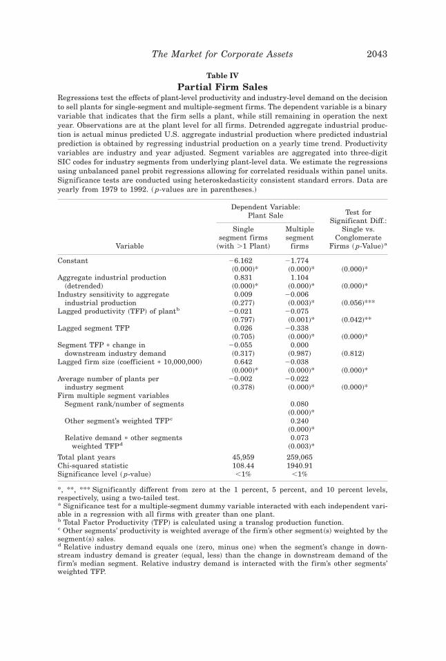
Table IV

Partial Firm SalesRegressions test the effects of plant-level productivity and industry-level demand on the decisionto sell plants for single-segment and multiple-segment firms. The dependent variable is a binaryvariable that indicates that the firm sells a plant, while still remaining in operation the nextyear. Observations are at the plant level for all firms. Detrended aggregate industrial produc-tion is actual minus predicted U.S. aggregate industrial production where predicted industrialprediction is obtained by regressing industrial production on a yearly time trend. Productivityvariables are industry and year adjusted. Segment variables are aggregated into three-digitSIC codes for industry segments from underlying plant-level data. We estimate the regressionsusing unbalanced panel probit regressions allowing for correlated residuals within panel units.Significance tests are conducted using heteroskedasticity consistent standard errors. Data areyearly from 1979 to 1992. ~ p-values are in parentheses.!

Dependent Variable:Plant Sale

Variable

Singlesegment firms

~with .1 Plant!

Multiplesegment

firms

Test forSignificant Diff.:

Single vs.Conglomerate

Firms ~ p-Value!a

Constant 26.162 21.774~0.000!* ~0.000!* ~0.000!*

Aggregate industrial production~detrended!

0.831 1.104~0.000!* ~0.000!* ~0.000!*

Industry sensitivity to aggregateindustrial production

0.009 20.006~0.277! ~0.003!* ~0.056!***

Lagged productivity ~TFP! of plantb 20.021 20.075~0.797! ~0.001!* ~0.042!**

Lagged segment TFP 0.026 20.338~0.705! ~0.000!* ~0.000!*

Segment TFP p change indownstream industry demand

20.055 0.000~0.317! ~0.987! ~0.812!

Lagged firm size ~coefficient p 10,000,000! 0.642 20.038~0.000!* ~0.000!* ~0.000!*

Average number of plants perindustry segment

20.002 20.022~0.378! ~0.000!* ~0.000!*

Firm multiple segment variablesSegment rank0number of segments 0.080

~0.000!*Other segment’s weighted TFPc 0.240

~0.000!*Relative demand p other segments

weighted TFPd0.073

~0.003!*

Total plant years 45,959 259,065Chi-squared statistic 108.44 1940.91Significance level ~ p-value! ,1% ,1%

*, **, *** Significantly different from zero at the 1 percent, 5 percent, and 10 percent levels,respectively, using a two-tailed test.a Significance test for a multiple-segment dummy variable interacted with each independent vari-able in a regression with all firms with greater than one plant.b Total Factor Productivity ~TFP! is calculated using a translog production function.c Other segments’ productivity is weighted average of the firm’s other segment~s! weighted by thesegment~s! sales.d Relative industry demand equals one ~zero, minus one! when the segment’s change in down-stream industry demand is greater ~equal, less! than the change in downstream demand of thefirm’s median segment. Relative industry demand is interacted with the firm’s other segments’weighted TFP.


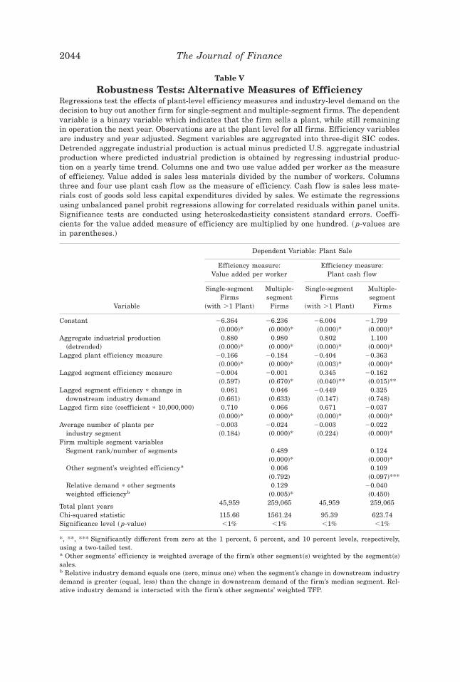
Table V

Robustness Tests: Alternative Measures of EfficiencyRegressions test the effects of plant-level efficiency measures and industry-level demand on thedecision to buy out another firm for single-segment and multiple-segment firms. The dependentvariable is a binary variable which indicates that the firm sells a plant, while still remainingin operation the next year. Observations are at the plant level for all firms. Efficiency variablesare industry and year adjusted. Segment variables are aggregated into three-digit SIC codes.Detrended aggregate industrial production is actual minus predicted U.S. aggregate industrialproduction where predicted industrial prediction is obtained by regressing industrial produc-tion on a yearly time trend. Columns one and two use value added per worker as the measureof efficiency. Value added is sales less materials divided by the number of workers. Columnsthree and four use plant cash f low as the measure of efficiency. Cash f low is sales less mate-rials cost of goods sold less capital expenditures divided by sales. We estimate the regressionsusing unbalanced panel probit regressions allowing for correlated residuals within panel units.Significance tests are conducted using heteroskedasticity consistent standard errors. Coeffi-cients for the value added measure of efficiency are multiplied by one hundred. ~ p-values arein parentheses.!

Dependent Variable: Plant Sale

Efficiency measure:Value added per worker

Efficiency measure:Plant cash f low

Variable

Single-segmentFirms

~with .1 Plant!

Multiple-segment

Firms

Single-segmentFirms

~with .1 Plant!

Multiple-segment

Firms

Constant 26.364 26.236 26.004 21.799~0.000!* ~0.000!* ~0.000!* ~0.000!*


0.880 0.980 0.802 1.100~0.000!* ~0.000!* ~0.000!* ~0.000!*

Lagged plant efficiency measure 20.166 20.184 20.404 20.363~0.000!* ~0.000!* ~0.003!* ~0.000!*

Lagged segment efficiency measure 20.004 20.001 0.345 20.162~0.597! ~0.670!* ~0.040!** ~0.015!**

Lagged segment efficiency p change indownstream industry demand

0.061 0.046 20.449 0.325~0.661! ~0.633! ~0.147! ~0.748!

Lagged firm size ~coefficient p 10,000,000! 0.710 0.066 0.671 20.037~0.000!* ~0.000!* ~0.000!* ~0.000!*


20.003 20.024 20.003 20.022~0.184! ~0.000!* ~0.224! ~0.000!*

Firm multiple segment variablesSegment rank0number of segments 0.489 0.124

~0.000!* ~0.000!*Other segment’s weighted efficiencya 0.006 0.109

~0.792! ~0.097!***Relative demand p other segmentsweighted efficiencyb

0.129 20.040~0.005!* ~0.450!

Total plant years 45,959 259,065 45,959 259,065

Chi-squared statistic 115.66 1561.24 95.39 623.74Significance level ~ p-value! ,1% ,1% ,1% ,1%

*, **, *** Significantly different from zero at the 1 percent, 5 percent, and 10 percent levels, respectively,using a two-tailed test.a Other segments’ efficiency is weighted average of the firm’s other segment~s! weighted by the segment~s!sales.b Relative industry demand equals one ~zero, minus one! when the segment’s change in downstream industrydemand is greater ~equal, less! than the change in downstream demand of the firm’s median segment. Rel-ative industry demand is interacted with the firm’s other segments’ weighted TFP.


are not productive, when their segment is less productive, and when thefirm has better performing assets elsewhere. This finding supports our Hy-potheses 2 and 3.

In Table VI we analyze the economic significance of our regression results.Specifically, we analyze how the probability of a sale by a single-segmentfirm or a division of a conglomerate varies as the level of industrial produc-tion and the productivity of the asset vary, holding all other variables attheir sample medians. The probability of a sale is derived using regressioncoefficients computed in Tables IV and V.

Panel A of Table VI shows how the probability that an asset is sold de-pends on the initial owner’s corporate structure and the asset’s productivity.In general, the probability that an asset is sold by a conglomerate firm ratherthan by a single-segment firm is higher by a factor of approximately four.Using our standard productivity measure, TFP, the probability that a me-dian level asset is sold by a conglomerate firm in any year is 3.71 percent,whereas the corresponding probability for a single-segment firm is 0.85 per-cent. Assets operated by peripheral divisions of conglomerates are sold at asomewhat higher rate.24 We also find that more efficient assets at the 90thpercentile have a lower probability of being sold than less efficient assets~10th percentile!. The results are not sensitive to the choice of productivitymeasure used. The table also shows that smaller peripheral divisions aremore likely to be sold. The probability a division with segment rank equal tothe 90th percentile is sold is 4.13 percent at the median productivity.

Panel B shows how variation in the real level of aggregate industrial pro-duction affects the probability of sale. We present results for the medianlevel of detrended industrial production and for levels that correspond to the90th and 10th percentiles, respectively. The rate of asset sales is very respon-sive to the variation in aggregate industrial production. Thus, for example,when the aggregate production is at the 90th percentile ~the second highestyear!, the probability that an asset of a conglomerate firm is sold is 4.03 per-cent, whereas it is only 3.20 percent when the level of industrial productionis at the 10th percentile ~the second lowest year!. The corresponding statis-tics for single-segment firms are 1.26 percent and 0.57 percent, again illus-trating their lower participation in the market for partial-firm asset sales.

Panel C shows the combined effect of the variation in productivity andaggregate industrial production. A low productivity plant owned by a periph-eral division of a conglomerate has a 4.82 percent probability of being soldwhen industrial production is high, whereas a high productivity plant at atime of low aggregate production has a probability of being sold of only 2.50percent. The corresponding probabilities for single-segment firms are 1.46percent and 0.48 percent, respectively.

24 The difference between single-segment and conglomerate rates may arise in part becausethe exit from an industry is classified as a partial-firm sale for a multisegment firm, but awhole-firm sale in the case of a single-segment firm. We return to this point in our discussionof Table IX.


Table VI

Probability of an Asset SalePredicted probability of an asset sale varying performance measures and industrial productionusing the regression coefficients from Tables IV and V. Panel A presents results varying per-formance measures from the 10th to 90th percentiles. Panel B presents results varying de-trended industrial production from its median value using yearly data from 1979 to 1992.Panel C varies both productivity and aggregate industrial production at their median values.We hold all other variables at their sample medians.

Panel A: Varying Initial Productivity0Performance

10thPercentile

MedianLevel

90thPercentile

Single-segment firmsVarying productivity ~Table IV, column 1! 1.08% 0.85% 0.66%Varying value added per worker ~Table V, column 1! 1.02% 0.88% 0.72%Varying cash f low ~Table V, column 3! 0.99% 0.87% 0.77%

Conglomerate firmsVarying productivity ~Table IV, column 2! 4.32% 3.71% 2.86%

Also decreasing segment rank to 10% ~main divisions! 4.11% 3.52% 2.71%Also increasing segment rank to 90% ~peripheral divisions! 4.80% 4.13% 3.20%

Varying value added per worker ~Table V, column 2! 4.06% 3.66% 3.08%Varying cash f low ~Table V, column 4! 4.19% 3.59% 3.04%

Panel B: Varying Industrial Production

10thPercentile

MedianLevel

90thPercentile

Single-segment firms~Table IV, column 1! 0.57% 0.85% 1.26%

Conglomerate firmsAll divisions ~Table IV, column 2! 3.20% 3.71% 4.03%


All divisions ~Table V, column 2! 3.21% 3.66% 4.09%All divisions ~Table V, column 4! 3.15% 3.59% 4.02%

Panel C: Varying Industrial Production and Productivity

Productivity10th andIndustrialProduction

90th percentileMeanLevel

Productivity90th andIndustrialProduction

10th percentile

Single-segment firmsVarying productivity ~Table IV, column 1! 1.46% 0.85% 0.48%Varying value added per worker ~Table V, column 1! 1.39% 0.88% 0.51%Varying cash f low ~Table V, column 3! 1.32% 0.87% 0.56%

Conglomerate firmsAll divisions ~Table IV, column 2! 4.82% 3.71% 2.50%


All divisions ~Table V, column 2! 5.53% 3.66% 2.70%All divisions ~Table V, column 4! 4.67% 3.59% 2.66%


Taken together, the estimates in Table VI suggest that the probability thata plant is transferred is considerably higher if the plant belongs to a multi-segment firm, particularly a small division of a multisegment firm. Ineffi-cient plants are more likely to be sold than efficient plants, and there areconsiderably more sales in times of high production. These observations areconsistent with the view that the market for plants facilitates the transferof assets to productive uses, and that transfers occur at times when themarginal value of capital is high. There is no evidence that managers ofconglomerate firms are less willing to sell assets than managers of single-segment firms.

D. Probability of Mergers and Acquisitions

In Table VII we analyze mergers and whole firm sell-offs. As before, wesplit the sample of selling firms into single-segment and multiple-segmentfirms. Because the majority of selling firms are small single-plant firms, wealso analyze these separately.

The results in Table VII show that industry demand strongly inf luencesmergers and acquisitions. The rate of mergers and firm sell-offs is higherwhen aggregate demand is high and in industries whose demand is sensitiveto aggregate output shocks. In contrast to the case of partial firm sales, therole of productivity in predicting mergers is less clear-cut. The probabilitythat a single-plant firm is sold decreases with its productivity. We find donot find similar significant effects with the sales of other firms. However,we do find that the probability that a multiple-segment firm is sold falls ifthe firm’s productivity is high and when the industries in which it operatesexperience higher demand. This finding is consistent with the first hypoth-esis in this paper, that firms are more likely to sell in good times when theyare less productive.

The significance of the relation between firm size and the probability ofsale also differs across the categories in Table VII. There is a significantpositive relation between firm size and the probability of sale for single-plant firms, no relation for multiple-plant single-segment firms, and a sig-nificant negative relation for multiple-segment firms. Controlling for size,focused firms are less likely to be sold then diversified firms.

E. Buyer Characteristics and the Probability of a Purchase

In Table VIII we examine the buyers of whole firms. We consider single-segment and multisegment firms separately. To investigate whether the mo-tives for focus-increasing and diversifying purchases are the same, we classifymultisegment buyers into those for whom the purchase increases firm focusand those for whom it decreases focus, as measured by the firm’s herfindahlindex across the segments it operates.

With only the exception of single-plant firms, we find that the probabilitythat a firm is a buyer in a particular industry increases with the buying


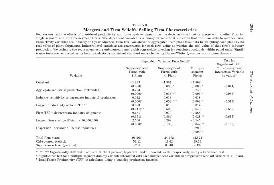
Table VII

Mergers and Firm Selloffs: Selling Firm CharacteristicsRegressions test the effects of plant-level productivity and industry-level demand on the decision to sell out or merge with another firm forsingle-segment and multiple-segment firms. The dependent variable is a binary variable that indicates that the firm sells to another firm.Productivity variables are industry and year adjusted. Firm-level variables are aggregated from plant-level data by weighting each plant by itsreal value of plant shipments. Industry-level variables are constructed for each firm using as weights the real value of that firm’s industryproduction. We estimate the regressions using unbalanced panel probit regressions allowing for correlated residuals within panel units. Signif-icance tests are conducted using heteroskedasticity-consistent standard errors following Huber–White. ~ p-values are in parentheses.!

Dependent Variable: Firm Selloff

Variable

Single-segmentFirms with

1 Plant

Single-segmentFirms with.1 Plant

Multiple-segment

Firms

Test forSignificant Diff.:Multiple-segment

Interaction Variable~ p-value!a

Constant 21.833 21.987 21.808~0.000! ~0.000!* ~0.000!* ~0.644!

Aggregate industrial production ~detrended! 0.723 0.716 0.743~0.000!* ~0.035!** ~0.006!* ~0.952!

Industry sensitivity to aggregate industrial production 0.012 0.013 0.018~0.000!* ~0.054!*** ~0.002!* ~0.519!

Lagged productivity of firm ~TFP!b 20.023 20.018 20.014~0.041!** ~0.526! ~0.549! ~0.600!

Firm TFP p downstream industry shipments 0.181 0.070 20.568~0.191! ~0.864! ~0.028!** ~0.615!

Lagged firm size ~coefficient p 10,000,000! 2.500 0.299 20.145~0.000!* ~0.186! ~0.042!** ~0.166!

Dispersion ~herfandahl! across industries 20.223~0.000!*

Total firm years 96,961 24,772 42,524Chi-squared statistic 56.12 11.62 39.36Significance level ~ p-value! ,1% 0.040 ,1%

*, **, *** Significantly different from zero at the 1 percent, 5 percent, and 10 percent levels, respectively, using a two-tailed test.a Significance test for a multiple-segment dummy variable interacted with each independent variable in a regression with all firms with .1 plant.b Total Factor Productivity ~TFP! is calculated using a translog production function.

2048T

he

Jou

rnal

ofF

inan

ce

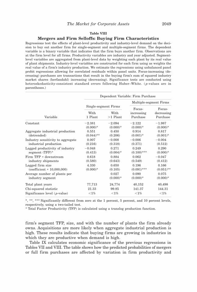
firm’s segment TFP, size, and with the number of plants the firm alreadyowns. Acquisitions are more likely when aggregate industrial production ishigh. These results indicate that buying firms are growing in industries inwhich they are productive when demand is high.

Table IX calculates economic significance of the previous regressions inTables VII and VIII. The table shows how the predicted probabilities of mergersor full firm purchases are affected by variation in firm productivity and

Table VIII

Mergers and Firm Selloffs: Buying Firm CharacteristicsRegressions test the effects of plant-level productivity and industry-level demand on the deci-sion to buy out another firm for single-segment and multiple-segment firms. The dependentvariable is a binary variable that indicates that the firm buys another firm. Observations areat the firm level for all firms. Productivity variables are industry and year adjusted. Segment-level variables are aggregated from plant-level data by weighting each plant by its real valueof plant shipments. Industry-level variables are constructed for each firm using as weights thereal value of a firm’s industry production. We estimate the regressions using unbalanced panelprobit regressions allowing for correlated residuals within panel units. Focus-increasing ~de-creasing! purchases are transactions that result in the buying firm’s sum of squared industrymarket shares ~herfandahl! increasing ~decreasing!. Significance tests are conducted usingheteroskedasticity-consistent standard errors following Huber–White. ~ p-values are inparentheses.!

Dependent Variable: Firm Purchase

Multiple-segment FirmsSingle-segment Firms

VariableWith

1 PlantWith

.1 Plant

Focus-increasingPurchase

Focus-decreasingPurchase

Constant 22.381 22.094 22.122 21.987~0.000!* ~0.000!* ~0.000!* ~0.000!*


0.551 0.450 0.914 0.817~0.044!** ~0.206! ~0.001!* ~0.001!*

Industry sensitivity to aggregateindustrial production

0.007 20.008 20.006 20.004~0.216! ~0.318! ~0.371! ~0.512!

Lagged productivity of industrysegment ~TFP!a

20.048 0.271 0.249 0.290~0.413! ~0.004!* ~0.100!*** ~0.000!*

Firm TFP p downstreamindustry shipments

0.618 0.884 0.062 20.047~0.580! ~0.643! ~0.549! ~0.412!

Lagged firm size~coefficient p 10,000,000!

4.330 0.650 0.196 0.166~0.000!* ~0.105! ~0.091!*** ~0.051!**


0.027 0.090 0.075~0.000!* ~0.000!* ~0.000!*

Total plant years 77,713 24,774 40,152 40,498Chi-squared statistic 21.33 99.85 141.37 144.31Significance level ~ p-value! ,1% ,1% ,1% ,1%

*, **, *** Significantly different from zero at the 1 percent, 5 percent, and 10 percent levels,respectively, using a two-tailed test.a Total Factor Productivity ~TFP! is calculated using a translog production function.


Table IX

Probability of MergersPredicted probability of a merger or full-firm purchase varying performance measures andindustrial production using the regression coefficients from Tables VII and VIII. Panel A presentsresults varying performance measures from the 10th to 90th percentiles. Panel B presentsresults varying detrended industrial production from its median value over 1979 to 1992. Panel Cvaries both productivity and aggregate industrial production at their median values. We holdall other variables at their sample medians.

Panel A: Selling Firms

Varying productivity 10th Percentile Median 90th Percentile

Single-segment selling firms 2.63% 2.55% 2.45%Conglomerate selling firms 3.21% 3.01% 2.77%

Varying industrial production 10th Percentile Median 90th Percentile


Varying productivity &industrial production

Productivity 10th,IndustrialProduction

90th PercentileMedianLevel


10th Percentile


Panel B: Buying Firms

Varying productivity 10th Percentile Median 90th Percentile

Single-segment buying firms 1.85% 2.13% 2.56%Conglomerate buying firms:

Focus increasing 2.30% 2.47% 2.94%Conglomerate buying firms:

Focus decreasing 2.92% 3.27% 3.95%

Varying industrial production 10th Percentile Median 90th Percentile




Varying productivity &industrial production


90th PercentileMedianLevel


10th Percentile





demand conditions. For the case of buying firms, the explanatory variablesand their variation parallel those discussed in the case of partial firm salesin Table VI.

Panel A shows the predicted probabilities of whole firms sales. As in thecase of partial firm sales, whole single-segment firms are less likely to besold than multisegment firms, at 2.55 percent and 3.01 percent, respectively.The difference between the two types of firms is less than the difference forasset sales. Taken together with the results on partial-firm sales in Table VII,our estimates predict that assets owned by conglomerate firms appear to be“in play” to a greater extent than assets owned by single-segment firms.Overall, predicted sales of multisegment firms are very sensitive to varia-tions in both productivity and aggregate industrial demand.

Panel B shows predicted variation in the probability of purchase. Again,the predicted purchases by multisegment firms are higher than by single-segment firms. The predicted probability that a firm is a buyer varies withthe firm’s productivity. However, the predicted probability that a multiseg-ment firm engages in a focus-decreasing purchase depends somewhat moreon the buying firm’s productivity. Both the probability of a purchase by asingle-segment firm and of a focus-decreasing purchase by a multisegmentfirm are also higher when aggregate industrial output is high. Focus-increasing mergers by multisegment firms are not as sensitive to changes inaggregate industrial production.

V. Are There Productivity Gains andWhat Determines the Gains?

In this section, we examine the productivity change ~industry adjusted ineach year! surrounding the asset sales—both for full-firm mergers and salesand for partial-firm sales. To begin the analysis, we first present simplesummary statistics on the change in productivity for the manufacturing plantsinvolved in purchases subsequent to the transactions.

In Table X, we analyze the changes in productivity using a three-by-threematrix to capture the internal organization characteristics of the buyer andthe seller. We classify both the buyer and the seller as a single-segmentfirm, or as a main or peripheral division of a multisegment firm. Becausethe results in Table VII suggest that single-plant firms may behave differ-ently than the rest of the firm population, in the case of mergers we furthersubclassify single-segment sellers into firms with one plant and firms withmore than one plant.

In this table, and in our subsequent tables analyzing productivity changes,we require that both buyer and seller ex ante data exist for each transaction.Transactions for which we have no ex ante data for buying firms includeforeign firms purchasing assets for the first time in the United States, non-manufacturing firms purchasing manufacturing assets, new firms formed topurchase existing assets, assets spun off or carved out from existing firms,


and small firms outside of the ASM sample that purchase larger plants.Given that our subsequent regressions analyze the effect of differences be-tween ex ante buyer and seller productivity, we also only analyze transac-tions for which we have ex ante productivity data for both buying and selling

Table X

Summary Statistics for Change in Productivityfor Assets Sold or Merged

The change in productivity, industry and year adjusted, for three years surrounding asset sales,mergers, or full-firm sales ~year 21 to year 12!. Values represent sample means for transac-tions between buyers and sellers. ~Standard error of the mean in parentheses.! Third row is thenumber of plants transacted.

Panel A: Partial-Firm Sales

Selling Firm Characteristics

Multidivision Firm

MainDivision

PeripheralDivision

Single-segmentFirm

Buying firm characteristicsMultidivision buyer adds to

Main division 0.062 0.103* 0.127~0.039! ~0.036! ~0.092!444 580 87

Peripheral division 20.008 0.047** 0.033~0.027! ~0.021! ~0.076!857 1,544 122

Single-segment buyer 0.019 0.107** 20.038~0.052! ~0.042! ~0.069!275 382 126

Panel B: Full-Firm Mergers and Acquisitions

Selling Firm Characteristics

Multidivision Firm Single-segment Firm

MainDivision

PeripheralDivision

with1 Plant

with.1 Plant

Buying firm characteristicsMultidivision buyer adds to

Main division 0.087** 0.143*** 20.020 20.039~0.041! ~0.083! ~0.039! ~0.043!

396 89 420 234Peripheral division 20.017 20.020 20.051*** 0.058

~0.020! ~0.025! ~0.028! ~0.039!1,278 914 723 401

Single-segment buyer 20.044 0.037 0.053 20.011~0.049! ~0.067! ~0.029! ~0.050!

237 108 677 219

*, **, *** Significantly different from zero at the 1 percent, 5 percent, and 10 percent levels,respectively, using a two-tailed test.


firms.25 After these requirements are taken into account, we are able toanalyze productivity changes for 10,109 transactions.

We calculate the industry adjusted change in productivity from the yearbefore the transaction to two years after the transaction, year 21 to year12, where year 0 is the year of the transaction. For our sample, the meanindustry adjusted change in productivity is 0.02, and is significantly differ-ent from zero at the one percent significance level. The median change inproductivity is also positive. Thus, the majority of the transactions in oursample have led to increases in productivity. Productivity changes for thetransaction types are given in Table X.

Panel A of Table X presents the change in productivity for partial-firmasset sales. We find that all sales from peripheral divisions have significantpositive ex post changes in productivity, regardless of the buyer’s organiza-tional characteristics. For single-segment sellers, no transactions resultedin a significant increase in productivity. There is no evidence that anycategory of transactions leads to significant declines in productivity of theassets sold.

Panel B presents the change in productivity for full-firm sales and merg-ers. Several facts emerge: We find significant productivity gains only whenbuyers add capacity to their main divisions—increasing the focus of theirfirm. Purchases by single-segment firms, although very frequent, do notresult in increased productivity of the purchased assets. Thus, there is evi-dence that restructuring that involves sales from multisegment firms to single-segment firms does not result in gains. Productivity significantly decreasesin only one class of transactions: purchases of single-plant firms by the pe-ripheral divisions of multisegment firms.

The differences in the observed gains in Table X may exist because sometypes of buyers are more efficient in improving assets. The differences mayalso occur if, in some types of transactions, there is a higher incidence ofinefficient sellers and efficient buyers, who have the expertise or resourcesto improve the assets. To examine the latter possibility, we classify transac-tions into those where the productivity of the buyer’s assets in the industryexceeds that of the acquired plants, and into those where it does not.

For partial-firm asset sales, the buyer’s existing plants are more produc-tive than the acquired plants in 59.6 percent of the transactions. For merg-ers and acquisitions, 57.2 percent of the total transactions have buyers thatare more productive than the plants they purchase. These proportions aresignificantly different from each other at the 1.5 percent level. Looking atdifferences based on firm organization, we also find significant differences.For example, for asset sales, we find that when firms add assets to theirmain divisions, their existing plants are more productive in 62.9 percent ofthe transactions. By contrast, for peripheral divisions 59.6 percent of buyersare more productive than purchased plants and for single segment firms

25 This also eliminates transactions occurring prior to 1979, given that we calculate produc-tivity in each industry using five years of lagged data.


54.9 percent are more productive than the purchased plants. In all cases theproportion of transactions is significantly greater than 50 percent at the1 percent level.

We next examine if these differences between the buyer’s and seller’s pro-ductivity significantly affect productivity gains of the purchased plants in amultivariate regression. To test whether the transaction type affects produc-tivity gains after controlling for productivity differences, we also allow for adifferential effect for the difference in seller and buyer productivity based onthe type of transaction. We regress the change in productivity of the pur-chased plants on the difference between the initial productivity of the buyerand the productivity of the plants purchased, buyer’s and the seller’s respec-tive firm sizes, and the selling firm’s initial productivity.

We expect the productivity of acquired plants to increase when they areacquired by a buyer who has higher productivity. However, the productivityof acquired plants may not increase when the buyer’s productivity is lower.To examine whether this occurs, we interact the difference between buyerand seller productivity with an indicator variable that equals one when thepurchased plant is more productive than the buyer. This variable allows theslope coefficient on the difference in buyer and seller productivity to changewhen buyers are less productive than the plants they purchase.

Lastly, to test whether there is a differential affect by type of transaction,we interact the difference in productivity between the buyer and seller withindicator variables identifying the different transaction categories fromTable X. The interaction variables measure how the effect of the differencebetween the buyer’s and seller’s initial productivity on the asset’s change inproductivity depends on whether the transaction is a partial sale or a merger,and on the organizational structure of the buyer and the seller. The interactionvariables thus allow different types of transactions to have larger or smallersensitivities to the difference between initial buyer and seller productivity.

Table XI shows that the productivity gain following a transaction dependson the productivities of the selling and buying firms. Assets increase in pro-ductivity when the productivity of the buying firm is higher than the pro-ductivity of the assets purchased. This finding suggests that the earlier stockmarket evidence of Lang, Stulz, and Walkling ~1989!, which shows total stockmarket gains of tender offers when high q firms acquire low q targets, is notcaused just by tax differences or by purely financial gains. However, whenassets are purchased by a buyer with a lower productivity, the purchasedassets’ productivity falls. Gains in productivity are positively related to theseller’s size and inversely related to the initial seller productivity.

None of the 17 estimated transaction interaction variables is statisticallysignificant. Thus, there is little evidence that the type of transaction affectsproductivity gains, after controlling for the initial buyer’s and seller’sproductivity.

The fact that some buyers acquire assets that are more productive thantheir existing assets, and that the acquired assets’ productivity declines sub-sequently, may initially appear puzzling. One possible explanation is that


Table XI

Change in Productivity Based onBuying & Selling Firm Characteristics

This table presents a single regression that tests the joint effects of buyer and selling firm organizationcharacteristics on the change in plant productivity over a three-year horizon from the year prior to the assetsale or merger ~year 21! to the end of the second year ~year 12! after the transaction. Total Factor Produc-tivity ~TFP! variables are calculated using a translog production function. Lagged firm productivity variablesare aggregated up from individual plants. All productivity variables are industry and year adjusted. Trans-action type variables are indicator variables that show whether the transaction was from a seller’s main orperipheral division or from a single-segment firm to a buyer’s main, peripheral, or to a single-segment buyer.Transaction type dummy variables are then interacted with the difference in productivity between the buyingfirm and the assets purchased. We estimate the regressions using ordinary least squares. Significance testsare conducted using heteroskedasticity-consistent standard errors. ~ p-values in parentheses.!

Dependent Variable:Change in Productivity Year 21 to 12

Transaction Type

Variable Partial Firm Sale Merger0Acquisition

Productivity and transaction sizeLagged productivity ~year 21!

of selling firm’s plants20.453~0.000!*

Difference in productivity ~year 21!

buying firm—productivity of plants purchased0.399

~0.000!*Difference in productivity ~year 21! p Indicator

variable for negative difference in productivity20.084~0.004!*

Buyer size ~coefficient p 10,000,000! 20.003~0.834!

Seller size ~coefficient p 10,000,000! 0.123~0.000!*

Difference in productivity interacted withtransaction characteristics

Sale from seller’s main divisionto buyer’s main division

20.009 0.000~0.931! ~0.907!

Sale from seller’s main divisionto buyer’s peripheral division

20.014 20.043~0.894! ~0.676!

Sale from seller’s main divisionto a single segment buyer

20.032 20.119~0.776! ~0.282!

Sale from seller’s peripheral divisionto buyer’s main division

0.119 omitted~0.268!

Sale from seller’s peripheral divisionto buyer’s peripheral division

20.002 20.058~0.987! ~0.572!

Sale from seller’s peripheral divisionto a single segment buyer

20.090 20.165~0.400! ~0.179!

Sale from single segment firmto buyer’s main division

0.021 20.034~0.883! ~0.750!

Sale from single segment firmto buyer’s peripheral division

0.065 20.045~0.620! ~0.662!

Sale from single segment firmto a single segment buyer

20.034 20.155~0.786! ~0.131!

Constant 20.066~0.000!*

Total transactions:Partial firm sales and merger and acquisitions 10,109R2 0.21F-test all coefficients 5 0 ~ p-value! ,1%

* Significantly different from zero at the 1 percent levels using a two-tailed test.


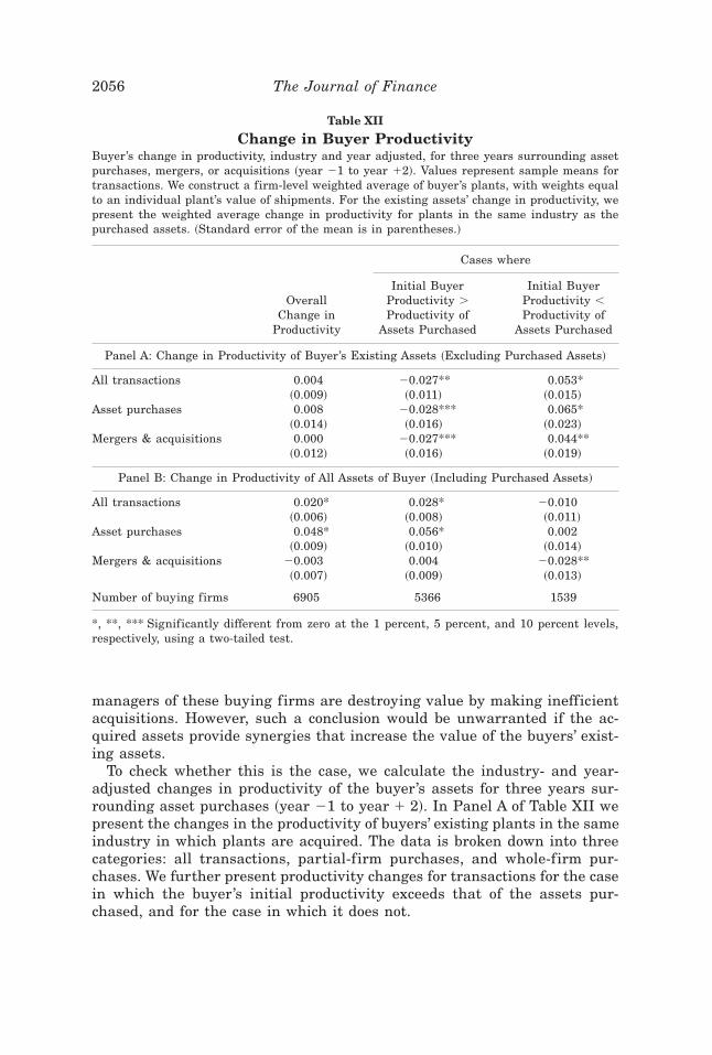
managers of these buying firms are destroying value by making inefficientacquisitions. However, such a conclusion would be unwarranted if the ac-quired assets provide synergies that increase the value of the buyers’ exist-ing assets.

To check whether this is the case, we calculate the industry- and year-adjusted changes in productivity of the buyer’s assets for three years sur-rounding asset purchases ~year 21 to year 1 2!. In Panel A of Table XII wepresent the changes in the productivity of buyers’ existing plants in the sameindustry in which plants are acquired. The data is broken down into threecategories: all transactions, partial-firm purchases, and whole-firm pur-chases. We further present productivity changes for transactions for the casein which the buyer’s initial productivity exceeds that of the assets pur-chased, and for the case in which it does not.

Table XII

Change in Buyer ProductivityBuyer’s change in productivity, industry and year adjusted, for three years surrounding assetpurchases, mergers, or acquisitions ~year 21 to year 12!. Values represent sample means fortransactions. We construct a firm-level weighted average of buyer’s plants, with weights equalto an individual plant’s value of shipments. For the existing assets’ change in productivity, wepresent the weighted average change in productivity for plants in the same industry as thepurchased assets. ~Standard error of the mean is in parentheses.!

Cases where

OverallChange in

Productivity

Initial BuyerProductivity .Productivity of

Assets Purchased

Initial BuyerProductivity ,Productivity of

Assets Purchased

Panel A: Change in Productivity of Buyer’s Existing Assets ~Excluding Purchased Assets!

All transactions 0.004 20.027** 0.053*~0.009! ~0.011! ~0.015!

Asset purchases 0.008 20.028*** 0.065*~0.014! ~0.016! ~0.023!

Mergers & acquisitions 0.000 20.027*** 0.044**~0.012! ~0.016! ~0.019!

Panel B: Change in Productivity of All Assets of Buyer ~Including Purchased Assets!

All transactions 0.020* 0.028* 20.010~0.006! ~0.008! ~0.011!

Asset purchases 0.048* 0.056* 0.002~0.009! ~0.010! ~0.014!

Mergers & acquisitions 20.003 0.004 20.028**~0.007! ~0.009! ~0.013!

Number of buying firms 6905 5366 1539

*, **, *** Significantly different from zero at the 1 percent, 5 percent, and 10 percent levels,respectively, using a two-tailed test.


Panel A shows that for all transactions, and for partial- and whole-firmtransactions taken separately, there is no overall change in the produc-tivity of the buyers’ existing assets in the same industry. However, thebuyers’ assets exhibit a significant decline in productivity in those caseswhere the initial buyers’ productivity exceeds that of the purchased assets.By contrast, buyers’ existing assets in a segment show a significant in-crease in productivity when more productive plants are acquired in thatsegment.

The pattern of gains is consistent with the notion that the addition of aless productive plant to a segment increases control costs and lowers theproductivity of existing assets. A majority of transactions are of this type.The fact that the acquisition of a more productive plant results in gains tothe existing assets and a decline in productivity of the acquired plants isconsistent with buyer purchasing expertise or productive ability that can betransferred to existing assets.

To determine whether the total gains in productivity outweigh the losses,we compute the total changes in the productivity of the buying firm aroundthe period of the transaction. This calculation, which includes the purchasedassets, shows the full effect of the purchase on all of the buyer’s manufac-turing operations. To get a firm-level measure of the productivity gain, weconstruct a weighted average of all plants of the buyer. We weight eachplant’s productivity by its initial value of shipments.

Panel B shows the buyers’ total productivity gains at the firm level. Theresults show that there is a significant firm-level productivity gain in partial-firm sales when the buyer’s productivity exceeds the productivity of the ac-quired plants. Thus, the productivity gain of the acquired plant~s! outweighsthe productivity loss on the firm’s existing assets. Panel B also shows that asignificant firm-level productivity loss only occurs in the case when lessproductive firms acquire more productive firms. In this case, the productiv-ity gain that the buying firm experiences is outweighed by the loss in pro-ductivity of the assets purchased. There are no signif icant f irm-levelproductivity effects in whole-firm sales when the buyer is more efficientthan the seller, or in partial-firm sales when the buyer acquires more effi-cient plants.

These results, combined with the summary statistics that show signifi-cant increases in productivity, are consistent with the hypothesis that themarket for assets works well for asset sales and for the majority of mergers.Assets that are transacted result in significant gains, consistent with Hy-pothesis 1 presented earlier. Contrary to the hypothesis that these divi-sions get subsidized by their parent firms, multidivisional firms are morelikely to sell less productive divisions and these sales to other firms resultin subsequent productivity increases. Our results support the conclusionthat assets change hands as the prospects in the overall economy and intheir other industries improve and their owners discover that they do nothave a comparative advantage in running these assets. There is signifi-cant firm-level fall in productivity surrounding a transaction in cases where


more efficient firms are acquired by less efficient firms—a minority oftransactions.26

Overall these results show that, as suggested by our first hypothesis,there are significant gains for assets being redeployed from less productivesellers to productive buyers. The results on the timing of transactions areconsistent with our second hypothesis, which predicts that more productivefirms will expand their operations in good times and when their prospectsin a given industry look better than the other industries in which theyoperate.

VI. Conclusions

In this paper, we analyze the market for corporate assets ~plants, divi-sions, and whole firms! in manufacturing industries. We analyze both thebuyers and sellers. We show that the market for both full and partial firmsis extensive. On average, 3.89 percent of plants change ownership in eachyear in our study. The total number of transactions varies with the economyand is strongly procyclical. In expansion years, close to 7 percent of plantsannually change ownership. Approximately the same number of plants aresold through partial-firm asset sales as in mergers and acquisitions. Thebuyers and sellers in the partial-firm asset sale market are typically largemultisegment firms, in contrast to the merger and acquisition market wherethe buyers are much bigger than the sellers.

We analyze the factors that are associated with the probability that assetstransfer ownership. We have three main results on the probability assets aresold:

1. For multiple-division firms, the probability of a firm selling assets de-creases with both the asset’s and the segment’s productivity. The prob-ability that assets are sold is higher for peripheral divisions. Theprobability of mergers and firm sell-offs is higher when the sellingfirm is less productive and the industry experiences a positive demandshock.

2. The selling firm’s productivity in other divisions impacts the probabil-ity of a sale. A division is more likely to be sold the better the prospectsof the other divisions.

3. We find that the probability that a firm is a buyer of additional assetsincreases with its efficiency and size.

26 In unreported results, we have also calculated the total effect of acquisitions at the seg-ment level. These calculations measure the changes of productivity of the new and existingassets of the segment that acquires the new assets. The qualitative results at the segment levelare the same as the results at the firm level.


In addition, we show that ex post productivity changes occur for assetstransacted and these productivity changes are associated with buyer andseller initial productivity and firm organization. We also examine the overallchanges in buyer productivity for purchasing firms. Our primary findingsfor changes in productivity for assets transacted are:

1. The gain in productivity of assets under new ownership is higher whenthe selling firm’s productivity is low and is higher the more productivethe buyer.

2. A firm’s internal organization is also associated with observed changesin productivity of the asset sold. Asset sales from peripheral divisionsof sellers to both main and peripheral divisions of buyers show signif-icant productivity gains. For mergers and acquisitions, assets that areacquired by the buyer’s main divisions from other multiple-segmentfirms show significant gains. These gains are primarily explained bythe differences in the initial productivity of buying and selling divisions.

3. When we take into account both the purchased and existing assets, thechange in productivity is positive for partial-firm asset purchases andis insignificantly different from zero for mergers and acquisitions.

4. When firms purchase assets of lower productivity, existing assets in-crease in productivity but the acquired assets decline in productivity.At the firm level, these losses on the acquired assets are offset by theproductivity increases of the purchased assets. Overall firm productiv-ity increases for partial-firm purchases and is insignificant for merg-ers and acquisitions.

5. When firms purchase assets of higher productivity, the acquired assetsdecline and the existing assets increase in productivity. At the firmlevel, the change in productivity is not significantly different from zerofor partial-firm purchases by less efficient producers. Firm-level pro-ductivity declines for one category of transactions: mergers and acqui-sitions by less efficient firms.

These findings suggest that firms have differing levels of ability to exploitassets, and that their comparative advantage is in their main industries.The low productivity of firms’ peripheral divisions prior to the sale, however,does not necessarily imply inefficient ownership. They may optimally oper-ate these divisions until demand is high, at which point more efficient buy-ers acquire these assets.

The productivity gains we document are consistent with buying firms be-ing able to offer a premium in part because of the gains in real productivitythat occur. The results are also consistent with more skilled buying firmsbeing able to transfer skill and improve the assets they purchase. There isno evidence that managers of conglomerate firms are less willing to sellassets than managers of single-segment firms.

The timing of sales and the pattern of productivity gains suggests thatmost transactions that occur in the market for plants and divisions tend toimprove the allocation of resources and are consistent with profit maximiz-


ing by firms across the divisions they operate. Thus, the pattern is consis-tent with profit-maximizing behavior. However, our results do not disprovethe existence of agency conf licts within firms. We identify one category oftransactions, full-firm acquisitions by buyers with lower productivity thanthat of the assets they purchase, for which overall firm productivity de-clines. Moreover, if managers are able to appropriate the gains of produc-tivity from any acquisitions, there might not be a gain to shareholders.

Our results would indicate that efficient firms refocusing in booms mayproduce the highest gains to transactions. Boards of directors should be morewilling to accept productivity explanations for these types of transactions,particularly for partial firm acquisitions.

Despite our finding that most transactions result in gains in productivity,this does not refute the proposition that sometimes managers undertaketransactions that, even given rational expectations, reduce value at the timethe transaction is undertaken. For example, our research would also suggestthat mergers and acquisitions by inefficient firms, presumably with lower stockmarket valuations relative to industry peers, should receive closer scrutinyby boards of directors. Further research should examine the link betweenacquirer and seller stock market valuations and subsequent productivity gains.

Overall, our results suggest that most transactions in the market for as-sets result in an increase in productive efficiency. We conclude that the mar-ket for corporate assets facilitates the redeployment of assets from firmswith a lower ability to exploit them to firms with higher ability.

Appendix

In estimating the TFPs in our sample, we use data for approximately 50,000plants each year. We are able to calculate lagged productivity for plants from1979 to 1992 as we use five years of lagged data to calculate productivity. Inthe productivity regression for each industry, we include three different typesof inputs: capital, labor, and materials, as explanatory variables for eachplant. All these data exist at the plant level. We include plants if plants haveat least two years of data. In addition, all observations must have nonzerovalues for all inputs and outputs. After productivity is calculated, we reportand use these numbers in regressions after excluding the top and bottomone percent of the calculated productivities. We also only include plants ifthe total value of firm shipments is at least 10 million real 1982 dollars.27

After imposing these restrictions, we end up with over 400,000 plant-levelproductivity measures.28 In calculating productivity, the capital variable used

27 We also find similar results changing this requirement to one million real 1982 dollars.28 The regressions in Table IV use 305,024 observations. Single-plant firms, representing

95,916 observations, are not included in Table IV. In addition, 15,874 observations are excludedas we also exclude outliers based on alternative measures of efficiency presented in Table V.The tables for mergers use firm-level observations obtained by aggregating these plant-levelobservations up to the firm level.


is plant’s capital stock that is available to be used in production. To accountfor depreciation of beginning of period capital stock, we use data from theBureau of Economic Analysis to make depreciation adjustments for begin-ning period capital stock at the two-digit level. To the beginning of periodcapital stock, we add the real dollars ~in real 1982 dollars! spent on capitalexpenditures for additions to the capital stock. In addition, to capture vin-tage effects of capital, we include plant age in our productivity calculations.Plant age is either the first year in which the plant appeared in the data-base, or 1972 ~the first year of the database!, if the plant existed in 1972.For the dependent variable, output, the ASM does not state the actual quan-tity shipped by each plant, but shows only the value ~in current period dol-lars! of shipments. We adjust all nominal dollar variables for inf lation byusing four-digit SIC code price def lators for output, materials, and capitalfrom the Bartelsman and Gray ~1994! database. Kovenock and Phillips ~1997!describe these inputs and the method for accounting for inf lation and de-preciation of capital stock in more detail.

To measure the productivity for a firm’s entire business segment, we con-struct a weighted average of individual plant productivity, in which the weightsare the predicted plant-level real value of shipments. The variable for theproductivity of the firm’s other segments is the weighted average of all of thefirm’s other plants outside of the segment in question. Again, the weightsare the predicted plant-level real value of shipments.

Figure A1. Histogram of R-squares from TFP within regressions run each year usingfive years of lagged data.


We also include other firm and segment-level variables in our regressionsto provide additional controls for unmeasured productivity differences andother factors, such as size, that can inf luence firm growth. We include thelagged firm size and the number of plants operated by a firm at the begin-ning of the year. We define firm size as the total value of shipments in real1982 dollars. We exclude all industry segments with real value of shipmentssmaller than one million dollars from our regressions.

Table AI

Total Factor ProductivityTable reports mean coefficients from yearly regressions by industry. Each regression is re-peated in each year for each industry using the last five years of data. Coefficients in columnone represent the average coefficients from regressions estimated in each year for each indus-try ~1,726 total regressions!. Columns two and three represent illustrative industries for 1978.In each year, productivity is the residual plus the firm-specific fixed effect obtained from re-gressing the real value ~def lated! of output on a plant’s age, the value of materials and inputs,the real value of a plant’s capital stock and the hours of labor utilized. Adjustments for depre-ciation for capital stock are made each year using depreciation def lators from the Bureau ofEconomic Analysis. All dollar amounts are def lated to 1982 dollars using def lators for theNational Bureau of Economic Research. ~ p-values in parentheses!.

Independent Variable: Real Value of Output

VariableMean

CoefficientMeat Packing

SIC 2011Oil Refining

SIC 2911

Age 0.013 0.019 0.169~0.061!*** ~0.587! ~0.009!*

Inputs 0.108 0.003 1.661~0.000!* ~0.972! ~0.000!*

Capital stock 0.044 0.084 0.306~0.000!* ~0.124! ~0.001!*

Labor 0.674 0.773 20.072~0.000!* ~0.000!* ~0.600!

~Inputs!2 0.074 20.001 0.009~0.000!* ~0.825! ~0.043!**

~Capital stock!2 0.000 0.075 0.007~0.631! ~0.000!* ~0.411!

~Labor!2 0.020 0.085 20.024~0.000!* ~0.000!* ~0.039!**

Inputs * capital stock 20.029 20.005 0.003~0.000!* ~0.640! ~0.856!

Inputs * labor 20.110 20.005 20.040~0.000!* ~0.503! ~0.003!*

Capital stock * labor 0.044 20.144 20.000~0.000!* ~0.000!* ~0.999!

Constant 3.352 2.819 23.765~0.000!* ~0.000!* ~0.000!*

R2 0.92 0.74

*, **, *** For column one mean value of the coefficient is significantly different from zero at the1, 5, 10 percent levels, respectively, using a two-tailed t-test. For columns two and three, sig-nificance test is whether coefficient is significantly different from zero using a two tailed t-test.


To allow for technical change, each regression is repeated for each indus-try for each year using data for the current year and the preceding fouryears, giving us a rolling panel of data for each year. Thus we can calculateproductivity for the 1978 to 1992 period. We use the earlier years of data,1974 to 1977, only for calculating the first year of productivity.29 Thus, thereare 1,726 separate regressions. Figure A1 shows the distribution of adjustedR2 for the regressions.

In Table AI we present the means of the coefficients for the 1,726 separateregressions covering the whole sample and also the coefficients for two sam-ple industries.

The coefficients for the sample industries are for 1979, the first year forwhich a five-year panel is available. The first industry, SIC 2011 Meat Pack-ing, was selected because it is the first industry in our sample when indus-tries are ranked by SIC codes. Because meat packing is labor intensive, thesecond industry, SIC 2911 Oil Refining was selected to illustrate a capitalintensive industry. The means of the coefficients in the whole sample aresignificantly different from zero. The coefficients of the two sample indus-tries ref lect their technologies. As expected, labor inputs have a more sig-nificant role in the meat packing equation and capital stock inputs are moreimportant in oil refining.

REFERENCES

Alexander, Gordon J., George P. Benson, and Joan M. Kampmeyer, 1984, Investigating thevaluation effects of announcements of voluntary corporate selloffs, Journal of Finance 39,503–517.

Andrade, Gregor, and Erik Stafford, 1999, Investigating the economic role of mergers, Workingpaper, Harvard Business School.

Baily, Martin Neil, Eric J. Bartelsman, and John Haltiwanger, 1998, Labor productivity: Struc-tural change and cyclical dynamics, Working paper 98-7, Center for Economic Studies.

Bartelsman, Eric J., Ricardo J. Caballero, and Richard K. Lyons, 1994, Customer and supplier-driven externalities, American Economic Review 84, 1075–1084.

Bartelsman, Eric J., and Wayne Gray, 1994, The NBER Manufacturing Productivity Database,Working paper, The Center for Economic Studies.

Caves, Richard E., and David R. Barton, 1990, Efficiency in U.S. manufacturing. ~MIT Press,Cambridge, MA!

Chevalier, Judith, 1999, Why do firms undertake diversifying mergers? An examination of theinvestment policies of merging firms, Mimeo, University of Chicago.

Fluck, Zsuzsanna, and Anthony W. Lynch, 1999, Why do firms merge and then divest: A theoryof financial synergy, Journal of Business 72, 319–346.

Graham, John, Michael Lemmon, and Jack Wolf, 2002, Does corporate diversification destroyvalue? forthcoming, Journal of Finance 57.

Hart, Oliver, and John Moore, 1995, Debt and seniority: An analysis of the role of hard claimsin constraining management, American Economic Review 85, 567–585.

29 In an earlier version of this paper, we calculated TFPs using the entire sample period foreach industry. The two methodologies yielded very similar qualitative results.


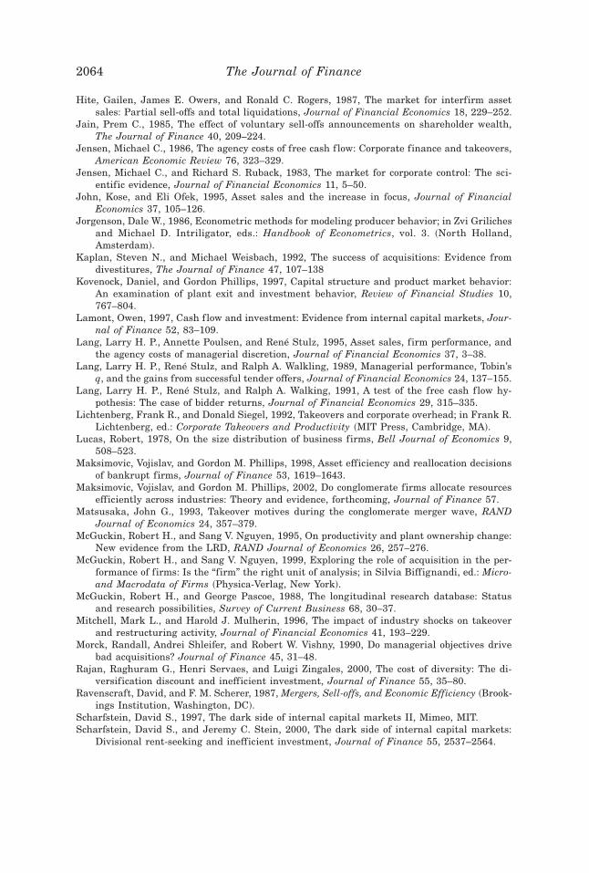
Hite, Gailen, James E. Owers, and Ronald C. Rogers, 1987, The market for interfirm assetsales: Partial sell-offs and total liquidations, Journal of Financial Economics 18, 229–252.

Jain, Prem C., 1985, The effect of voluntary sell-offs announcements on shareholder wealth,The Journal of Finance 40, 209–224.

Jensen, Michael C., 1986, The agency costs of free cash f low: Corporate finance and takeovers,American Economic Review 76, 323–329.

Jensen, Michael C., and Richard S. Ruback, 1983, The market for corporate control: The sci-entific evidence, Journal of Financial Economics 11, 5–50.

John, Kose, and Eli Ofek, 1995, Asset sales and the increase in focus, Journal of FinancialEconomics 37, 105–126.

Jorgenson, Dale W., 1986, Econometric methods for modeling producer behavior; in Zvi Grilichesand Michael D. Intriligator, eds.: Handbook of Econometrics, vol. 3. ~North Holland,Amsterdam!.

Kaplan, Steven N., and Michael Weisbach, 1992, The success of acquisitions: Evidence fromdivestitures, The Journal of Finance 47, 107–138

Kovenock, Daniel, and Gordon Phillips, 1997, Capital structure and product market behavior:An examination of plant exit and investment behavior, Review of Financial Studies 10,767–804.

Lamont, Owen, 1997, Cash f low and investment: Evidence from internal capital markets, Jour-nal of Finance 52, 83–109.

Lang, Larry H. P., Annette Poulsen, and René Stulz, 1995, Asset sales, firm performance, andthe agency costs of managerial discretion, Journal of Financial Economics 37, 3–38.

Lang, Larry H. P., René Stulz, and Ralph A. Walkling, 1989, Managerial performance, Tobin’sq, and the gains from successful tender offers, Journal of Financial Economics 24, 137–155.

Lang, Larry H. P., René Stulz, and Ralph A. Walking, 1991, A test of the free cash f low hy-pothesis: The case of bidder returns, Journal of Financial Economics 29, 315–335.

Lichtenberg, Frank R., and Donald Siegel, 1992, Takeovers and corporate overhead; in Frank R.Lichtenberg, ed.: Corporate Takeovers and Productivity ~MIT Press, Cambridge, MA!.

Lucas, Robert, 1978, On the size distribution of business firms, Bell Journal of Economics 9,508–523.

Maksimovic, Vojislav, and Gordon M. Phillips, 1998, Asset efficiency and reallocation decisionsof bankrupt firms, Journal of Finance 53, 1619–1643.

Maksimovic, Vojislav, and Gordon M. Phillips, 2002, Do conglomerate firms allocate resourcesefficiently across industries: Theory and evidence, forthcoming, Journal of Finance 57.

Matsusaka, John G., 1993, Takeover motives during the conglomerate merger wave, RANDJournal of Economics 24, 357–379.

McGuckin, Robert H., and Sang V. Nguyen, 1995, On productivity and plant ownership change:New evidence from the LRD, RAND Journal of Economics 26, 257–276.

McGuckin, Robert H., and Sang V. Nguyen, 1999, Exploring the role of acquisition in the per-formance of firms: Is the “firm” the right unit of analysis; in Silvia Biffignandi, ed.: Micro-and Macrodata of Firms ~Physica-Verlag, New York!.

McGuckin, Robert H., and George Pascoe, 1988, The longitudinal research database: Statusand research possibilities, Survey of Current Business 68, 30–37.

Mitchell, Mark L., and Harold J. Mulherin, 1996, The impact of industry shocks on takeoverand restructuring activity, Journal of Financial Economics 41, 193–229.

Morck, Randall, Andrei Shleifer, and Robert W. Vishny, 1990, Do managerial objectives drivebad acquisitions? Journal of Finance 45, 31–48.

Rajan, Raghuram G., Henri Servaes, and Luigi Zingales, 2000, The cost of diversity: The di-versification discount and inefficient investment, Journal of Finance 55, 35–80.

Ravenscraft, David, and F. M. Scherer, 1987, Mergers, Sell-offs, and Economic Efficiency ~Brook-ings Institution, Washington, DC!.

Scharfstein, David S., 1997, The dark side of internal capital markets II, Mimeo, MIT.Scharfstein, David S., and Jeremy C. Stein, 2000, The dark side of internal capital markets:

Divisional rent-seeking and inefficient investment, Journal of Finance 55, 2537–2564.


Schlingemann, Frederik, P., René M. Stulz, and Ralph A. Walkling, 2002, Asset liquidity andsegment divestitures, forthcoming , Journal of Financial Economics.

Shea, John, 1993, Do supply curves slope up? Quarterly Journal of Economics 108, 1–32.Shleifer, Andrei, and Robert W. Vishny, 1992, Liquidation values and debt capacity: A market

equilibrium approach, Journal of Finance 47, 1343–1365.Williamson, Oliver, 1985, The Economic Institutions of Capitalism: Firms, Markets, Relational

Contracting, The Free Press, New York.


the market for corporate assets: who engages in mergers...

Documents