1

Introduction

The analytical solution of the atmospheric diffusion equation has been containing different shaped depending on Gaussian and non- Gaussian solutions. An analytical solution with power law for the wind speed and eddy diffusivity with the realistic assumption was studied by [1]the solution has been implemented in the KAPPA-G model [2],and [3] extended the solution of [1] under boundary conditions suitable for dry deposition at the ground. The mathematics of atmospheric dispersion modeling is studied by [4]. In the analytical solutions of the diffusion-advection

equation, assuming constant along the whole planetary boundary layer (PBL) or following a power law was studied by [5-7], [2] and[8].

Estimating of crosswind integrated Gaussian and non-Gaussian concentration through different dispersion schemes is studied by [9].Analytical solution of diffusion equation in two dimensions using two forms of eddy diffusivities is studied by[9]. In this paper the advection diffusion equation (ADE) is solved in two directions to obtain crosswind integrated ground level

ISSN: 2347-3215 Volume 2 Number 5 (May-2014) pp. xx-xx www.ijcrar.com

A B S T R A C T

The advection diffusion equation (ADE) is solved in two directions to obtain the crosswind integrated concentration. The solution is solved using Laplace transformation technique and considering the wind speed depends on the vertical height and eddy diffusivity depends on downwind and vertical distances. We compared between the two predicted concentrations and observed concentration data are taken on the Copenhagen in Denmark.

KEYWORDS

Advection Diffusion Equation, Laplace Transform, Predicted Normalized Crosswind Integrated Concentrations

The Mathematical Modelingof the Atmospheric Diffusion Equation

1Khaled. S.M. Essa*, 2M.M.Abdel El-Wahab, 3H.M.ELsman, 4A.Sh.Soliman, 5S.M.ELgmmal and 6A.A.Wheida

1Department of Mathematics and Theoretical Physics, Nuclear Research Centre, Atomic Energy Authority, Cairo, Egypt 2Astronmy department, Faculty of science, Cairo university, Egypt 3,5 Physics department, Faculty of science, Monofia university, Egypt 4,6Theoretical physics department, National Research Center, Cairo, Egypt

*Corresponding author email: mohamedksm56@yahoo.com

2

concentration in unstable conditions. We use Laplace transformation technique and considering the wind speed and eddy diffusivity depends on the vertical height and downwind distance. We compare between observed data from Copenhagen (Denmark) and predicted concentration data using statistical technique.

Analytical Method

Time dependent advection

diffusion equation is written as [10]

where: C is the average concentration of air pollution ( g/m3).

u is the mean wind speed (m/s). ,

and are the eddy diffusivities coefficients along x, y and z axes respectively (m2/s).

For steady state, taking , and the diffusion in the x-axis direction is assumed to be zero compared with the advective in the same directions, hence:

(2)

We must

assumethat , integrating the equation (2) with respect to y,we obtain the normalized crosswind integrated concentration of contaminant from - to

at a point of the atmospheric advection diffusion equation is written in the form [11];

(3)

Equation (3) is subjected to the following boundary conditions

i. It is assumed that the pollutants are reflected at the ground surface

i.e.

ii. The flux at the top the mixing layer can be given by

Where h is the mixing height

iii. The mass continuity is written in the form:-

( , )y suC x z Q z h at 0x wherQ is

the source strength, is Dirac delta function and sh is the stake height.

The concentration of the pollutant tends to zero at large distance of the source, i.e.

( , ) 0yC x z at z

If L is the operator of the Laplace transform then;

0

( , ) ( , )sxy yC s z e C x z dx Applying the

Laplace transform on equation (3) to have: 2

2

( , )( , ) ( , )y

y y

C s zK suC s z uC x z

zFromboundary condition (iii)this equation becomes

2

2

( , )( , )y

y s

C s zK suC s z Q z h

z

3

Dividing on K to obtain;

2

2

( , )( , )y

y s

C s z su QC s z z h

K Kz(4)

To find particular solution put 0s

Qz h

Kthen;

2

2

( , )( , ) 0y

y

C s z suC s z

Kz(5)

The nonhomogeneous partial differential equation has a solution in the form of particular solution plus complementary solution, particular solution has the following form:

1 2( , )su su

z zK K

yC s z C e C e (6)

And complementary solution;

1 2( , )su su

z zK K

yC s z C z e C z e (7)

Using properties of partial differential equations[12]to obtain:

1 2 0su su

z zK KC z e C z e (8)

And 1 2

su suz z

K Ks

su suC z e C z e Q z h

K K(9)

Multiplying equation (8) by su

Kto obtain

1 2 0su su

z zK Ksu su

C z e C z eK K

(10)

Summing equations (9) and (10) to obtain

2

2

suz

Ks

QC z e z h

suK

K

by integrating

20 0

2

s ssu

zh hK

s

QC z dz e z h dz

suK

K

Then 2 22

ssu

hKQ

C z esuK (11)

From equation (8)we can deduce that 1 2

su suz z

K KC z e C z e

Substituting by 2C z then 12

suz

Ks

QC z e z h

suKby integrating then

4

1 1

2

ssu

hKQ

C z esuK

(12)

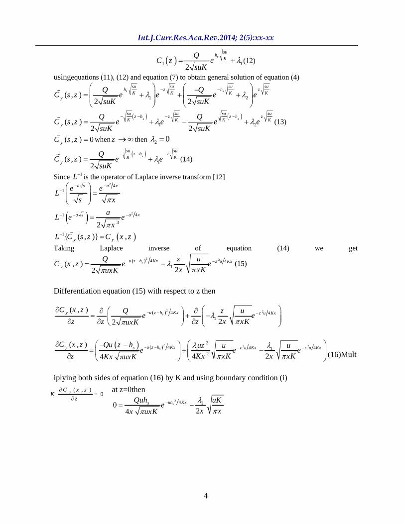
usingequations (11), (12) and equation (7) to obtain general solution of equation (4)

1 2( , )2 2

s ssu su su su

h z h zK K K K

y

Q QC s z e e e e

suK suK

1 2( , )2 2

s s

su su su suz h z z h z

K K K Ky

Q QC s z e e e e

suK suK(13)

( , ) 0yC s z when z then 2 0

1( , )2

s

su suz h z

K Ky

QC s z e e

suK(14)

Since 1L is the operator of Laplace inverse transform [12] 2

2

41

1 4

3

1

2

{ ( , )} ,

a s a x

a s a x

y y

e eL

s x

aL e e

x

L C s z C x z

Taking Laplace inverse of equation (14) we get 2 24 4

1( , )22

su z h Kx z u Kxy

Q z uC x z e e

x xKuxK(15)

Differentiation equation (15) with respect to z then

2 24 41

( , )

22su z h Kxy z u KxC x z Q z u

e ez z z x xKuxK

2 2 22

4 4 41 12

( , )

4 24su z h Kxy s z u Kx z u KxC x z Qu z h uz u u

e e ez Kx xK x xKKx uxK (16)Mult

iplying both sides of equation (16) by K and using boundary condition (i)

at z=0then 2 4 10

24suh KxsQuh uK

ex xx uxK

( , )0yC x z

Kz

5

2

2

4 1

41

24

2

4

s

s

u h K xs

u h K xs

Q u h u Ke

x xx u x K

x Q u h xe

u Kx u x K

2 4

1 2suh KxsQuh

euK

Substituting with in equation (14) to obtain

2 2 24 4 4( , )2 22

s su z h Kx uh Kx z u Kxsy

QuhQ z uC x z e e e

uK x xKuxK

2 22 44( , )22

ssu z h Kxu z h Kx s

y

uzhQC x z e e

xKuxK

2 22 441( , )

22ss

u z h Kxu z h Kx sy

uzhC x z Q e e

xKuxK (17)

In unstable case we take the value of the vertical eddy diffusivity in the

form 1v

zK z k w z

h(18)

Substituting from equation (18) in equation (3), we get that:

2

2

21 1

( ) ( )y y y

v vC C C

x zz

z zk w z k w

h hu z u z

(19)

Applying the Laplace transform on equation (19) respect to x and considering that:

0

( , ) { , ; }

( , ) ,

y p y

sxy y

C s z L C x z x s

C s z e C x z dx

, 0,p y yC

L sC s z C zx

(20)

2 22 44( , )2 2

ssu z h Kxu z h Kx s

y

QuzhQC x z e e

uxK xK uxK

6

WhereLp is the operator of the Laplace transform Substituting from (20) in equation (19), we obtain that:

2

2 2 2 2

* *

21, ,

, 0,y yy y

v v

zC s z C s z us uh

C s z C zzz z z z

z k w z k w zh h h

(21)

Substituting from (ii) in equation (21) we get:-

2

2 2 2 2

* *

21

, ,,

y y sy

v v

zC s z C s z Q z hush

C s zzz z z z

z k w z k w zh h h

(22)

After integrated equation (22) with respect to z, we obtain that:

**

ln,,

1

yy

svv s

z hu s

C s z QzC s z

hz k wk w h

h

(23)

Equation (23) is non homogeneous differential equation then, above equation has got two solutions, one is homogeneous and other is special solution, in order to solve the homogeneous,

we put,

* 1 sv s

Qh

k w hh

=0 in equation (23),the solution becomes:

*

l n

2

, v

z hs u

zz

k wyC s z

c eQ

(24)

After taking Laplace transform in equation (24) and substitute from (ii), we obtain that: -

21

sc z hu s

(25)

Substituting from equation (25) in equation (24) we get that:-

*

ln

, 1

s

s

v

h hs u

hz

k w

yC s ze

Q u s(26)

7

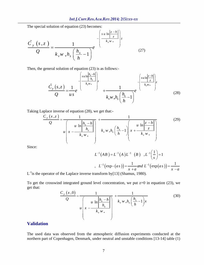
The special solution of equation (23) becomes:

*

ln

, 1

1

v

z hs u

zz

k wy

sv s

C s ze

hQk w h

h

(27)

Then, the general solution of equation (23) is as follows:-

* *

ln ln

, 1 1

1

s

s

v v

h h z hsu suh zz zk w k wy

sv s

C s ze e

hQ u sk w h

h

(28)

Taking Laplace inverse of equation (28), we get that:- , 1 1

lnln1

y

s

ssv s

vv

C x z

Q z hh h uu h zh k w h xu x h k wk w

(29)

Since:

1 1 1 1

1 1

1, 1

1 1, exp exp

L AB L A L B Ls

L a s and L a sx a x a

L-1is the operator of the Laplace inverse transform by[13] (Shamus, 1980).

To get the crosswind integrated ground level concentration, we put z=0 in equation (23), we get that:

,0 1 1

1ln

y

ssv s

s

v

C x

hQ h h k w h xuhh

u xk w

(30)

Validation

The used data was observed from the atmospheric diffusion experiments conducted at the northern part of Copenhagen, Denmark, under neutral and unstable conditions [13-14] table (1)

8

shows that the comparison between observed, predicted model 1 and predicted model integrated crosswind ground level concentrations under unstable condition and downwind distance.

Cy/Q *10-4 (s/m3) Run no.

Stability Down distance

(m) Observed Predicted model 1

K(x) = 0.16 ( w2/u) x.

Predicted model 2 K(z)=kv w* z (1-z /h)

1 Very unstable (A) 1900 6.48 4.469878 5.01 1 Very unstable (A) 3700 2.31 2.295811 2.62 2 Slightly unstable (C) 2100 5.38 3.135609 4.36 2 Slightly unstable (C) 4200 2.95 1.568679 2.26

3 Moderately unstable (B) 1900 8.2 5.454451 5.01 3 Moderately unstable (B) 3700 6.22 2.802046 2.61 3 Moderately unstable (B) 5400 4.3 1.920065 1.80 5 Slightly unstable (C) 2100 6.72 7.136663 4.50 5 Slightly unstable (C) 4200 5.84 2.364105 2.27 5 Slightly unstable (C) 6100 4.97 1.627889 1.57 6 Slightly unstable (C) 2000 3.96 4.961762 4.35 6 Slightly unstable (C) 4200 2.22 1.261926 2.21 6 Slightly unstable (C) 5900 1.83 0.898436 1.60 7 Moderately unstable (B) 2000 6.7 2.647701 4.57 7 Moderately unstable (B) 4100 3.25 1.976309 2.32 7 Moderately unstable (B) 5300 2.23 1.52897 1.81 8 Neutral (D) 1900 4.16 4.26145 4.89 8 Neutral (D) 3600 2.02 2.719159 2.68 8 Neutral (D) 5300 1.52 1.847384 1.85 9 Slightly unstable (C) 2100 4.58 4.657708 4.34 9 Slightly unstable (C) 4200 3.11 1.712648 2.26 9 Slightly unstable (C) 6000 2.59 1.199 1.60

Fig.1 the variation of the tow predicted models ad observed via downwind distance

9

Fig. (1) Shows that the predicted normalized crosswind integrated concentrations values of the model 2are good to the observed data than the predicted of model 1.

Fig.2the variation between the two predicted models and observed concentrations.

Table (2) Comparison between our two models according to standard statistical Performance measure

Models NMSE FB COR FAC2 Predicated model 1 0.30 -0.40 0.78 1.56 Predicated model 2 0.26 0.32 0.67 0.80

Fig. (2) Shows that the predicted data of model 2 is nearer to the observed concentrations data than the predicted data of model 1. From the above figures, we find that there are agreement between the predicted normalized crosswind integrated concentrations of model 2 depends on the vertical height with the observed normalized crosswind integrated concentrations than the predicted model 1 which depends on the downwind distance.

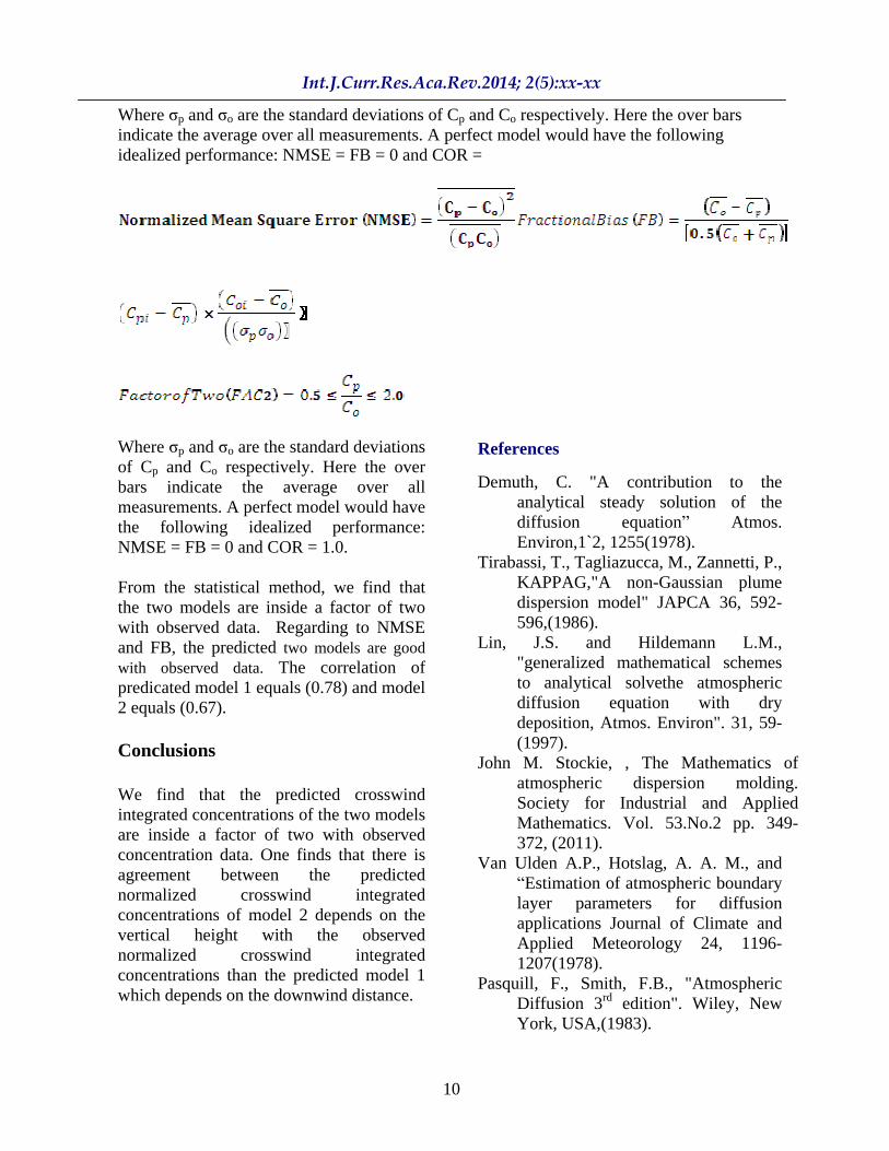
Statistical method

Now, the statistical method is presented and comparison between predicted and observed results will be offered by (Hanna, 1989).The following standard statistical performance measures that characterize the agreement between prediction (Cp=Cpred/Q) and observations (Co=Cobs/Q):

10

Where p and o are the standard deviations of Cp and Co respectively. Here the over bars indicate the average over all measurements. A perfect model would have the following idealized performance: NMSE = FB = 0 and COR =

Where p and o are the standard deviations of Cp and Co respectively. Here the over bars indicate the average over all measurements. A perfect model would have the following idealized performance: NMSE = FB = 0 and COR = 1.0.

From the statistical method, we find that the two models are inside a factor of two with observed data. Regarding to NMSE and FB, the predicted two models are good with observed data. The correlation of predicated model 1 equals (0.78) and model 2 equals (0.67).

Conclusions

We find that the predicted crosswind integrated concentrations of the two models are inside a factor of two with observed concentration data. One finds that there is agreement between the predicted normalized crosswind integrated concentrations of model 2 depends on the vertical height with the observed normalized crosswind integrated concentrations than the predicted model 1 which depends on the downwind distance.

References

Demuth, C. "A contribution to the analytical steady solution of the diffusion equation Atmos. Environ,1`2, 1255(1978).

Tirabassi, T., Tagliazucca, M., Zannetti, P., KAPPAG,"A non-Gaussian plume dispersion model" JAPCA 36, 592-596,(1986).

Lin, J.S. and Hildemann L.M., "generalized mathematical schemes to analytical solvethe atmospheric diffusion equation with dry deposition, Atmos. Environ". 31, 59-(1997).

John M. Stockie, , The Mathematics of atmospheric dispersion molding. Society for Industrial and Applied Mathematics. Vol. 53.No.2 pp. 349-372, (2011).

Van Ulden A.P., Hotslag, A. A. M., and Estimation of atmospheric boundary

layer parameters for diffusion applications Journal of Climate and Applied Meteorology 24, 1196- 1207(1978).

Pasquill, F., Smith, F.B., "Atmospheric Diffusion 3rd edition". Wiley, New York, USA,(1983).

11

Seinfeld, J.H Atmospheric Chemistry and

physics of Air Pollution . Wiley, New York,(1986).

Sharan, M., Singh, M.P., Yadav, A.K," Mathematical model for atmospheric dispersion in low winds with eddy diffusivities as linear functions of downwind distance". Atmospheric Environment 30, 1137-1145, (1996).

EssaK.S.M., and E,A.Found,"Estimated of crosswind integrated Gaussian and Non-Gaussian concentration by using different dispersion schemes". Australian Journal of Basic and Applied Sciences, 5(11): 1580-1587,(2011).

Arya, S. P"Modeling and parameterization of near source diffusion in weak wind" J.Appl.Met. 34, 1112-1122. (1995).

EssaK. S. M., Maha S. EL-Qtaify"Diffusion from a point source in an urban Atmosphere"Meteol.Atmo, Phys., 92, 95-101, (2006).

Shamus "Theories and examples in Mathematics for Engineering and Scientific"(1980).

Gryning S. E., and Lyck E Atmospheric dispersion from elevated sources in anurban area: Comparison between tracer experiments and model calculations , J. Climate Appl. Meteor., 23, pp. 651-660., (1984).

Gryning S.E., Holtslag, A.A.M., Irwin, J.S., Sivertsen, B., Applied dispersion modeling based on meteorological scaling parameters , Atoms. Environ. 21 (1), 79-89(1987).