the mathematical-physical theory of communication-observation

Latency-Information Theory The Mathematical-Physical Theory of Communication-Observation

Erlan H. Feria Department of Engineering Science and Physics, The City University of New York/CSI, USA

E Mail: [email protected] Web Site: http://feria.csi.cuny.edu

Abstract—In this paper the mathematical-physical theory of communication-observation that is part of latency-information theory (LIT) is reviewed. LIT surfaced from the confluence of classical information theory, relativity theory, quantum mechanics, statistical physics and a 1978 conjecture by the author of a structural-physical certainty-uncertainty duality for quantized control. Control, radar, physics and biochemistry applications illustrate the theory. As part of the review, LIT is revealed to communicate through latency-certainty channels and/or information-uncertainty channels for observation across latency-certainty sensors and/or information-uncertainty sensors, a mathematical-physical efficiency perspective of the Universe in a four quadrants revolution. While the first and third quadrants are concerned with the life time of physical signal movers and the life space of physical signal retainers, respectively, the second and fourth quadrants are about the intelligence space of mathematical signal sources and the processing time of mathematical signal processors, respectively. The four quadrants of LIT are conjectured to be physically independent with their system design methodologies guided by dualities and performance bounds. Moreover, the tools of statistical physics bridge them, and inherently lead to the discovery of a novel certainty dual for thermodynamics named lingerdynamics.

Keywords — latency-certainty, information-uncertainty, mathematical-intelligence, physical-life, communication-channel, observation-sensor, thermodynamics, lingerdynamics, biochemistry

I. INTRODUCTION The mathematical-physical theory of communication-

observation is part of latency-information theory (LIT) [1]. This universal efficiency theory emerged from the confluence of five ideas. They are in chronological order: 1) the certainty advocacy of Albert Einstein of relativity theory; 2) the uncertainty advocacy of Werner Heisenberg of quantum mechanics; 3) the source-entropy and channel-capacity lossless performance bounds of Claude Shannon that guide communication system designs [2]; 4) the thermodynamics-entropy of Steven Hawking for black-holes [3]-[4]; and 5) the 1978 conjecture of a structural-physical certainty/uncertainty duality for quantized control by the author [5].

In this review classical information theory will be designated as mathematical information theory (or MIT) since the units of classical information are mathematical binary digit

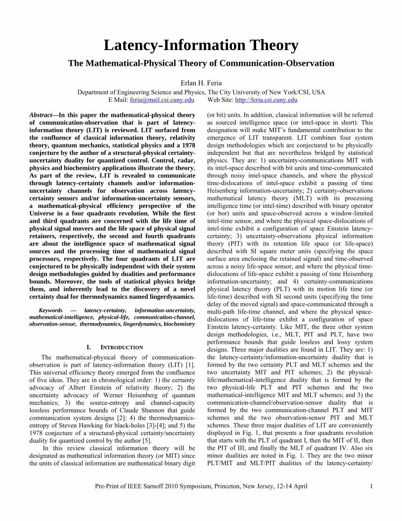
(or bit) units. In addition, classical information will be referred as sourced intelligence space (or intel-space in short). This designation will make MIT’s fundamental contribution to the emergence of LIT transparent. LIT combines four system design methodologies which are conjectured to be physically independent but that are nevertheless bridged by statistical physics. They are: 1) uncertainty-communications MIT with its intel-space described with bit units and time-communicated through noisy intel-space channels, and where the physical time-dislocations of intel-space exhibit a passing of time Heisenberg information-uncertainty; 2) certainty-observations mathematical latency theory (MLT) with its processing intelligence time (or intel-time) described with binary operator (or bor) units and space-observed across a window-limited intel-time sensor, and where the physical space-dislocations of intel-time exhibit a configuration of space Einstein latency-certainty; 3) uncertainty-observations physical information theory (PIT) with its retention life space (or life-space) described with SI square meter units (specifying the space surface area enclosing the retained signal) and time-observed across a noisy life-space sensor, and where the physical time-dislocations of life-space exhibit a passing of time Heisenberg information-uncertainty; and 4) certainty-communications physical latency theory (PLT) with its motion life time (or life-time) described with SI second units (specifying the time delay of the moved signal) and space-communicated through a multi-path life-time channel, and where the physical space-dislocations of life-time exhibit a configuration of space Einstein latency-certainty. Like MIT, the three other system design methodologies, i.e., MLT, PIT and PLT, have two performance bounds that guide lossless and lossy system designs. Three major dualities are found in LIT. They are: 1) the latency-certainty/information-uncertainty duality that is formed by the two certainty PLT and MLT schemes and the two uncertainty MIT and PIT schemes; 2) the physical-life/mathematical-intelligence duality that is formed by the two physical-life PLT and PIT schemes and the two mathematical-intelligence MIT and MLT schemes; and 3) the communication-channel/observation-sensor duality that is formed by the two communication-channel PLT and MIT schemes and the two observation-sensor PIT and MLT schemes. These three major dualities of LIT are conveniently displayed in Fig. 1, that presents a four quadrants revolution that starts with the PLT of quadrant I, then the MIT of II, then the PIT of III, and finally the MLT of quadrant IV. Also six minor dualities are noted in Fig. 1. They are the two minor PLT/MIT and MLT/PIT dualities of the latency-certainty/

Pre-Print of IEEE Sarnoff 2010 Symposium, Princeton, New Jersey, 12-14 April

1

mailto:[email protected]

http://feria.csi.cuny.edu/

2 2

3

3

1 1

Passing of Time Configuration of Space

of Time Dislocated Signals of Space Dislocated Signals“The Heisenberg Advocacy” “The Einstein Advocacy”

2 2

3

3

1 1

Passing of Time Configuration of Space

of Time Dislocated Signals of Space Dislocated Signals“The Heisenberg Advocacy” “The Einstein Advocacy”

Fig.1 The Latency-Information Theory Revolution

information-uncertainty major duality, then the two minor PLT/PIT and MIT/MLT dualities of the physical-life/mathematical-intelligence major duality and finally the two minor PLT/MLT and MIT/PIT dualities of the communication-channel/observation-sensor major duality.

II. THE LIT CONFLUENCE The chronological development of LIT is documented next. It starts with the two lossless efficiency performance bounds of MIT that led to the discovery of six others for LIT [6]. Next the conjectured structural-physical certainty/uncertainty duality is explained. Then a 2004-2005 DARPA University Grant for adaptive knowledge-aided radar system designs is discussed that motivated the confluence of MIT with the structural-physical certainty/uncertainty duality conjecture [7]. The section ends with the physical duals for MIT and MLT, i.e., PLT and PIT that were discovered in 2006.

A. The MIT Performance Bounds The first MIT performance bound is the lower

performance bound for source-coder designs, which is called the source-entropy with symbol H in bit units for the sourced intel-space quantity that it represents. H is defined as the expected source-information

Λ=== ∑Ω

= 21log)()()]([

i iSiSiS gIgPgIEH (1)

))(/1(log)( 2 iSiS gPgI = ∑Ω==Λ 1 )()(2 i iSiS gIgP (2)

where: 1) G {∈ g1,..,gΩ} is a n-dimensional random vector composed of Ω vector outcomes {g1,..,gΩ}; 2) IS(gi) is the gi source-information in bit units; 3) PS(gi) is the gi source-probability; and 4) Λ is viewed as an effective number of outcomes, with Λ=Ω for equally likely outcomes.

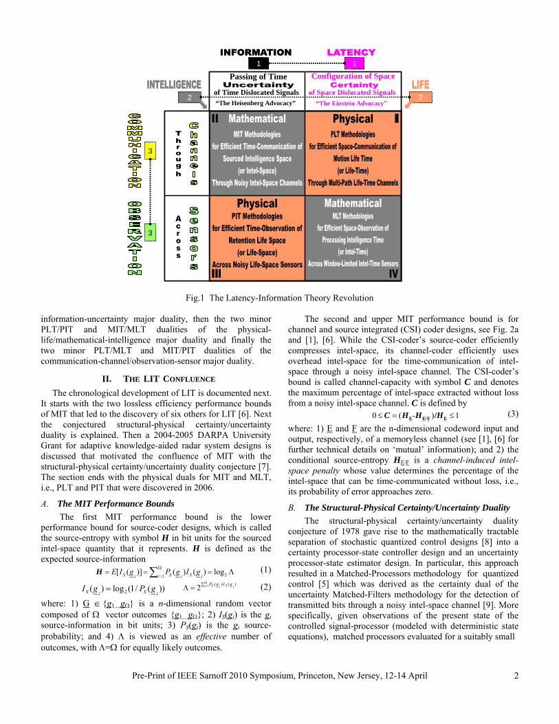
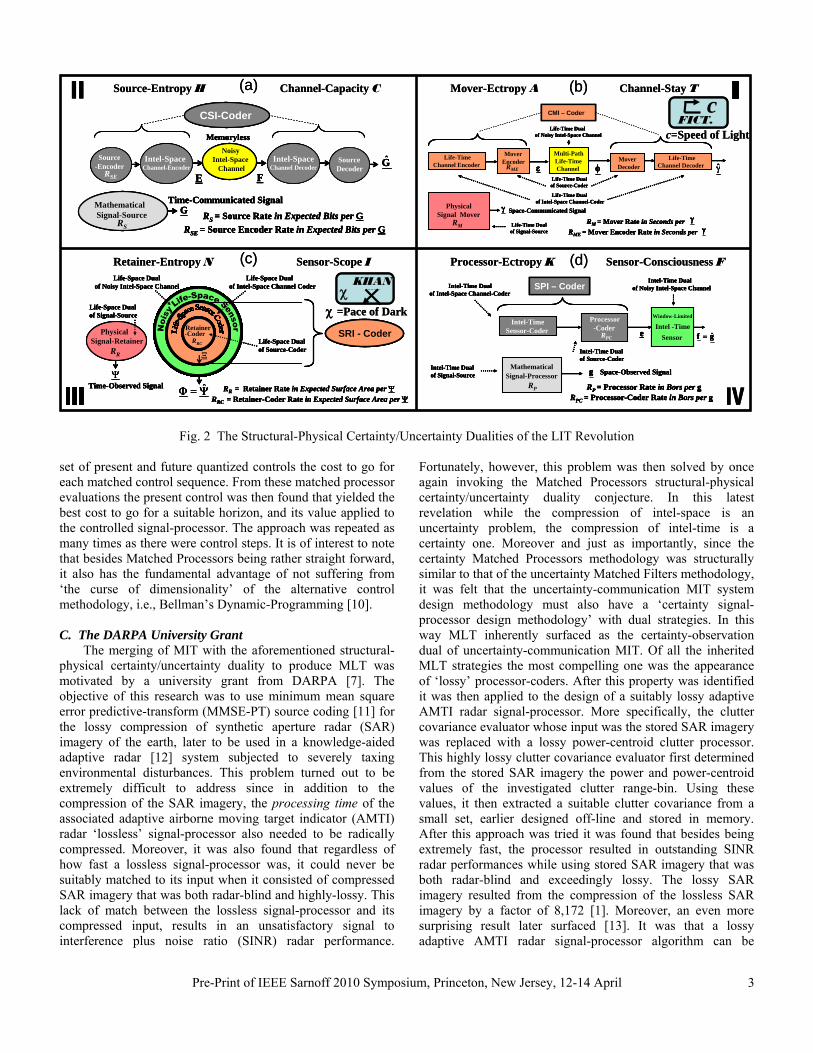
The second and upper MIT performance bound is for channel and source integrated (CSI) coder designs, see Fig. 2a and [1], [6]. While the CSI-coder’s source-coder efficiently compresses intel-space, its channel-coder efficiently uses overhead intel-space for the time-communication of intel-space through a noisy intel-space channel. The CSI-coder’s bound is called channel-capacity with symbol C and denotes the maximum percentage of intel-space extracted without loss from a noisy intel-space channel. C is defined by

1)(0 ≤=≤ EF/EE /HHHC - (3) where: 1) E and F are the n-dimensional codeword input and output, respectively, of a memoryless channel (see [1], [6] for further technical details on ‘mutual’ information); and 2) the conditional source-entropy HE/F is a channel-induced intel-space penalty whose value determines the percentage of the intel-space that can be time-communicated without loss, i.e., its probability of error approaches zero.

B. The Structural-Physical Certainty/Uncertainty Duality The structural-physical certainty/uncertainty duality

conjecture of 1978 gave rise to the mathematically tractable separation of stochastic quantized control designs [8] into a certainty processor-state controller design and an uncertainty processor-state estimator design. In particular, this approach resulted in a Matched-Processors methodology for quantized control [5] which was derived as the certainty dual of the uncertainty Matched-Filters methodology for the detection of transmitted bits through a noisy intel-space channel [9]. More specifically, given observations of the present state of the controlled signal-processor (modeled with deterministic state equations), matched processors evaluated for a suitably small


2

(a) (b)

(d)

RP = Processor Rate in Bors per gRPC = Processor-Coder Rate in Bors per g

Sensor-TimeIntel

Intel-Time Dualof Source-Coder

Intel-Time Dualof Intel-Space Channel-Coder

Intel-Time Dualof Noisy Intel-Space Channel

Intel-TimeSensor-Coder

SPI – Coder

Window-Limited

e gf ˆ=

Processor-Coder

g

RPC

MathematicalSignal-Processor

RP

Intel-Time Dualof Signal-Source Space-Observed Signal


Sensor-TimeIntel





SPI – Coder

Window-Limited

e gf ˆ=

Processor-Coder

g

RPC


RP


CSI-Coder

G

MathematicalSignal-Source

NoisyIntel-Space

ChannelE F

Source-Encoder

RS = Source Rate in Expected Bits per GRSE = Source Encoder Rate in Expected Bits per G

RS

RSE

Intel-SpaceChannel-Encoder

SourceDecoder

Intel-SpaceChannel Decoder

Memoryless

GTime-Communicated Signal

CSI-Coder

G


NoisyIntel-Space

ChannelE F

Source-Encoder


RS

RSE


SourceDecoder


Memoryless


Source-Entropy H Channel-Capacity C Mover-Ectropy A Channel-Stay T

Processor-Ectropy K Sensor-Consciousness F

FICT.c

c=Speed of Light

(c)Retainer-Entropy N Sensor-Scope I

KHANχ

χ =Pace of Dark

Life-Time Dualof Intel-Space Channel-Coder

Life-Time Dualof Source-Coder

Life-TimeChannel Encoder

MoverEncoder

Multi-Path Life-TimeChannel

Life-TimeChannel Decoder

MoverDecoder

CMI – Coder

Life-Time Dualof Noisy Intel-Space Channel

γRME

PhysicalSignal Mover

RM RM = Mover Rate in Seconds perRME = Mover Encoder Rate in Seconds per

γ

ε φ

γγ

Life-Time Dualof Signal-Source

Space-Communicated Signal




MoverEncoder



MoverDecoder

CMI – Coder


γRME



γ

ε φ

γγ



SRI - CoderLife-Space Dual of Source-Coder

Life-Space Dual of Intel-Space Channel Coder

Life-Space Dual of Noisy Intel-Space Channel

RR = Retainer Rate in Expected Surface Area per ΨRRC = Retainer-Coder Rate in Expected Surface Area per Ψ

RetainerCoder

RRC

RetainerCoderRetainerCoder

RetainerRetainerRetainerRetainer

Ξ

Ψ=Φ ˆ

-Coder

RR

RRC

Ψ

PhysicalSignal-Retainer

Life-Space Dualof Signal-Source

Time-Observed Signal

-





RetainerCoder

RRC




Ξ

Ψ=Φ ˆ

-Coder

RR

RRC

Ψ




-

(a) (b)

(d)


Sensor-TimeIntel





SPI – Coder

Window-Limited

e gf ˆ=

Processor-Coder

g

RPC


RP



Sensor-TimeIntel





SPI – Coder

Window-Limited

e gf ˆ=

Processor-Coder

g

RPC


RP


CSI-Coder

G


NoisyIntel-Space

ChannelE F

Source-Encoder


RS

RSE


SourceDecoder


Memoryless


CSI-Coder

G


NoisyIntel-Space

ChannelE F

Source-Encoder


RS

RSE


SourceDecoder


Memoryless


Source-Entropy H Channel-Capacity C Mover-Ectropy A Channel-Stay T

Processor-Ectropy K Sensor-Consciousness F

FICT.c

c=Speed of Light

(c)Retainer-Entropy N Sensor-Scope I

KHANχ

χ =Pace of Dark




MoverEncoder



MoverDecoder

CMI – Coder


γRME



γ

ε φ

γγ






MoverEncoder



MoverDecoder

CMI – Coder


γRME



γ

ε φ

γγ







RetainerCoder

RRC



Ξ

Ψ=Φ ˆ

-Coder

RR

RRC

Ψ




-





RetainerCoder

RRC




Ξ

Ψ=Φ ˆ

-Coder

RR

RRC

Ψ




-

Fig. 2 The Structural-Physical Certainty/Uncertainty Dualities of the LIT Revolution

set of present and future quantized controls the cost to go for each matched control sequence. From these matched processor evaluations the present control was then found that yielded the best cost to go for a suitable horizon, and its value applied to the controlled signal-processor. The approach was repeated as many times as there were control steps. It is of interest to note that besides Matched Processors being rather straight forward, it also has the fundamental advantage of not suffering from ‘the curse of dimensionality’ of the alternative control methodology, i.e., Bellman’s Dynamic-Programming [10]. C. The DARPA University Grant

The merging of MIT with the aforementioned structural-physical certainty/uncertainty duality to produce MLT was motivated by a university grant from DARPA [7]. The objective of this research was to use minimum mean square error predictive-transform (MMSE-PT) source coding [11] for the lossy compression of synthetic aperture radar (SAR) imagery of the earth, later to be used in a knowledge-aided adaptive radar [12] system subjected to severely taxing environmental disturbances. This problem turned out to be extremely difficult to address since in addition to the compression of the SAR imagery, the processing time of the associated adaptive airborne moving target indicator (AMTI) radar ‘lossless’ signal-processor also needed to be radically compressed. Moreover, it was also found that regardless of how fast a lossless signal-processor was, it could never be suitably matched to its input when it consisted of compressed SAR imagery that was both radar-blind and highly-lossy. This lack of match between the lossless signal-processor and its compressed input, results in an unsatisfactory signal to interference plus noise ratio (SINR) radar performance.

Fortunately, however, this problem was then solved by once again invoking the Matched Processors structural-physical certainty/uncertainty duality conjecture. In this latest revelation while the compression of intel-space is an uncertainty problem, the compression of intel-time is a certainty one. Moreover and just as importantly, since the certainty Matched Processors methodology was structurally similar to that of the uncertainty Matched Filters methodology, it was felt that the uncertainty-communication MIT system design methodology must also have a ‘certainty signal-processor design methodology’ with dual strategies. In this way MLT inherently surfaced as the certainty-observation dual of uncertainty-communication MIT. Of all the inherited MLT strategies the most compelling one was the appearance of ‘lossy’ processor-coders. After this property was identified it was then applied to the design of a suitably lossy adaptive AMTI radar signal-processor. More specifically, the clutter covariance evaluator whose input was the stored SAR imagery was replaced with a lossy power-centroid clutter processor. This highly lossy clutter covariance evaluator first determined from the stored SAR imagery the power and power-centroid values of the investigated clutter range-bin. Using these values, it then extracted a suitable clutter covariance from a small set, earlier designed off-line and stored in memory. After this approach was tried it was found that besides being extremely fast, the processor resulted in outstanding SINR radar performances while using stored SAR imagery that was both radar-blind and exceedingly lossy. The lossy SAR imagery resulted from the compression of the lossless SAR imagery by a factor of 8,172 [1]. Moreover, an even more surprising result later surfaced [13]. It was that a lossy adaptive AMTI radar signal-processor algorithm can be


3

designed that emulates the outstanding SINR radar performance of the former scheme without the need of clutter prior-knowledge, i.e., SAR imagery. This highly desirable result surfaced from the discovery that both the range-bin power and its power-centroid can be readily derived from the on-line sample covariance matrix.

D. The MLT Performance Bounds

Similarly to MIT, MLT is found to have two performance bounds for system designs [1], [6]. The first is the lower performance bound for processor-coder designs, which is called processor-ectropy with symbol K and values given in bor units for the processing intel-time levels that it represents. A processor-coder is any replacement of the original signal-processor whose output is said to be lossless when it matches that of the original signal-processor and lossy when it does not. More specifically K is a minimax criterion that is illustrated next with a simple example. This example is of a 1-bit full-adder [14] original signal-processor that has a slow bor multi-level implementation structure where the sum output is associated with six bor levels and the carry-out with five bor levels. The reason for this relatively large number of bor levels is that this full-adder only uses two-input gates. However, for this example it is found that K=3 bors since the minimum number of bor levels needed to generate the carry bit is two, and for the sum bit is three as is noted to be the case when a ‘sum of minterms’ implementation methodology is used [14] and more than two-input gates are allowed. While the 1-bit full adder is a lossless processor-coder, a lossy but faster, by one bor level, 1-bit full adder can be readily derived from the lossless case by only implementing the two bor levels for the carry and by setting the sum output to zero. Thus K is defined (4) )]]([)],..,([max[)](),..,(max[ 111 NPNPNPP gCfgCfgLgL ==Kwhere: a) g=[g1,..gN] is the N-dimensional signal-processor vector output; b) LP(gi) is the gi processor-latency, e.g. LP(sum)=3 bors for the full-adder; and c) fi[CP(gi)]=LP(gi) conveys LP(gi) dependence on gi processor-constraint CP(gi).

The second and upper MLT performance bound is for sensor and processor integrated (SPI) coder designs, see Fig. 2d and [1], [6]. While the SPI-coder’s processor-coder efficiently compresses intel-time, its sensor-coder efficiently uses overhead intel-time for the space-observation of intel-time across a window-limited intel-time sensor. The SPI-coder’s bound is called sensor-consciousness with symbol F and denotes the maximum percentage of the mathematical latency extracted without loss from a window-limited intel-time sensor. F is defined by

1)(0 ef/ee ≤=≤ KKKF /- (5) where: 1) e and f are N-dimensional vectors that are the input and output, respectively, of a window-limited intel-time sensor (see [1], [6] for further technical details on ‘mutual’ latency); and 2) the conditional processor-ectropy Ke/f is a sensor-induced intel-time penalty whose value determines the percentage of the intel-time that can be space-observed without loss. For instance, if a 1-bit full-adder based recursive adder contributes 2 bor levels of delay for each carry-out, its processor-ectropy is Ke=16 bors when it adds 8 bits. Then if

one observes the adder output with a 14-bors window-limited intel-time sensor, the sensor-induced inter-time penalty will be of 2 bor, i.e. Ke/f =2 bors. In turn, this results in the sensor-consciousness value of F=(16-2)/16=0.88 informing us that only 88% of the 16 bors intel-time of Ke can be space-observed without loss. Thus the adder intel-time must be of at least 18 bors. The needed 2 bors can be obtained with a sensor-coder that uses prior-knowledge, e.g. that LSBs can be zero, to begin the addition 2 bors earlier in time [1], [6]. E. The PIT and PLT Physical Duals In 2006 soon after the discovery of the MLT methodology as the certainty dual of the uncertainty MIT methodology, the physical duals for MIT and MLT were also revealed. These physical duals, i.e., PIT for MIT and PLT for MLT, lead to physical system designs that are once again guided by lower and upper performance bounds. Furthermore, the structural-physical certainty/uncertainty duality conjecture for PLT and PIT brings to mind classical themes from physics. The first is the certainty advocacy of Einstein for a perfectly described ‘certainty’ Universe of which his relativity theory was part. Yet it is also well known that the Heisenberg uncertainty principle is at the center of quantum mechanics, which never seems to fail in its description of the real-world for small distances. Thus for many years physicists have been busy in the search for a quantum theory of gravity at the Plank length where it is thought Einstein’s relativity theory yields to quantum mechanics [15]. A recent popular candidate for this theory is string theory with its conjectured eleven dimensions for the Universe as well as further generalizations. Yet, recently [15], experimental data from an exploding star has surfaced conveying a different perspective. This perspective is that the speed of light does not seem to change its value when its wavelength is at the Plank length, with further smaller wavelength results expected in the near future. The results obtained so far have already elicited comments from physicists such as “It would be amazing that in effect we don’t need a quantum theory of gravity,” [15]. Thus it seems that the structural-physical certainty/uncertainty duality conjecture has reasonable support. Retention problems of quantum mechanics may thus be found to form together with the motion problems of relativity theory a true duality where quantum mechanics and relativity theory complement each other and never merge. A desirable outcome of this scenario is that retention problems that are often severely limited in the type of experiments that can be performed, may nevertheless be studied using the structural-physical certainty/uncertainty duality. F. The PLT Performance Bounds

Similarly to MIT and MLT, PLT has been found to have two performance bounds for system designs. The first is the lower performance bound for mover-coder designs, which is called mover-ectropy with symbol A and values given in SI second units for the motion life-time interval that it represents. A mover-coder is any replacement of the original signal-mover of physical signals that is lossless when it moves the same physical signals moved by the original signal-mover and


4

lossy when it does not. Examples of mover-coders are four-wheeled vehicles used in the space-dislocation of people and photons that carry electromagnetic radiation at the speed of light in a vacuum. An example of a lossy mover-coder is an automobile that can only move six people, but yet replaces a van that carries ten people, thus the four people left behind represent a physical signal loss. Similar to the processor-ectropy K, the mover-ectropy A is a minimax criterion that can be conveniently illustrated with a computational device contained in a sphere. The computations start on one side of the sphere and end on the other side with a constant speed v of travel along all possible connecting paths. As a mover moves along one of these connecting paths at constant speed v binary operations are performed in cascade. A is then

A=πr/v (6) where r is the radius of the sphere. To derive this result it is first noted that πr/v is the minimum life-time for computations that are restricted to the surface of the sphere. On the other hand, 2r/v is the minimum life-time for computations that are not restricted as to which path may be taken. Notice that this minimum life-time path is along the diameter of the sphere whose distance is 2r. The largest of these two life-times, i.e. πr/v, is then the minimax mover-ectropy A. Thus A is defined )]]([)],..,([max[)](),..,(max[ 111 NMNMNMM CfCfLL γγγγ ==A (7)

where: a) γ=[γ1,..γN] is the N-dimensional signal-mover vector output; b) LM(γi) is the γi mover-latency, e.g. LM(surface path)= πr/v (where v=c for photon); and c) fi[CM(γi)]=LM(γi) conveys LM(γi) dependence on γi mover-constraint CM(γi).

The second and upper PLT performance bound is for channel and mover (CMI) coder designs, see Fig. 2b and [1], [6]. The c shown in Fig. 2b reminds us about the upper speed of light in a vacuum limit conjectured by Einstein that movers can never exceed. While the CMI-coder’s mover-coder efficiently compresses life-time, its channel-coder efficiently uses overhead life-time for the space-communication of life-time through a multi-path life-time channel. The CMI-coder’s bound is called channel-stay with symbol T and denotes the maximum percentage of the physical latency extracted without loss through a multi-path life-time channel. T is defined by

1)(0 ε/εε ≤=≤ AAAT /φ- (8)

where: 1) ε and φ are N-dimensional vectors that are the input and output, respectively, of a multi-path life-time channel; and 2) the conditional mover-ectropy Aε/φ is a channel-induced life-time penalty whose value determines the percentage of the life-time that can be space-communicated without loss. For instance, if a computational sphere yields 1.2 msec for its minimum surface path and 1 msec for its direct diameter path, Aε=1.2 msec. Then if the computations of each path are slowed down by a life-time channel that increases the computation life-time by at most 0.2 msec, it follows that Aε/φ =0.2 msec. In turn, this results in T=(1.2-0.2)/1.2=0.834 informing us that only 83.3% of the 1.2 msec life-time in Aε can be space-communicated without loss. Thus the spherical computer life-time must be of at least 1.4 msecs.

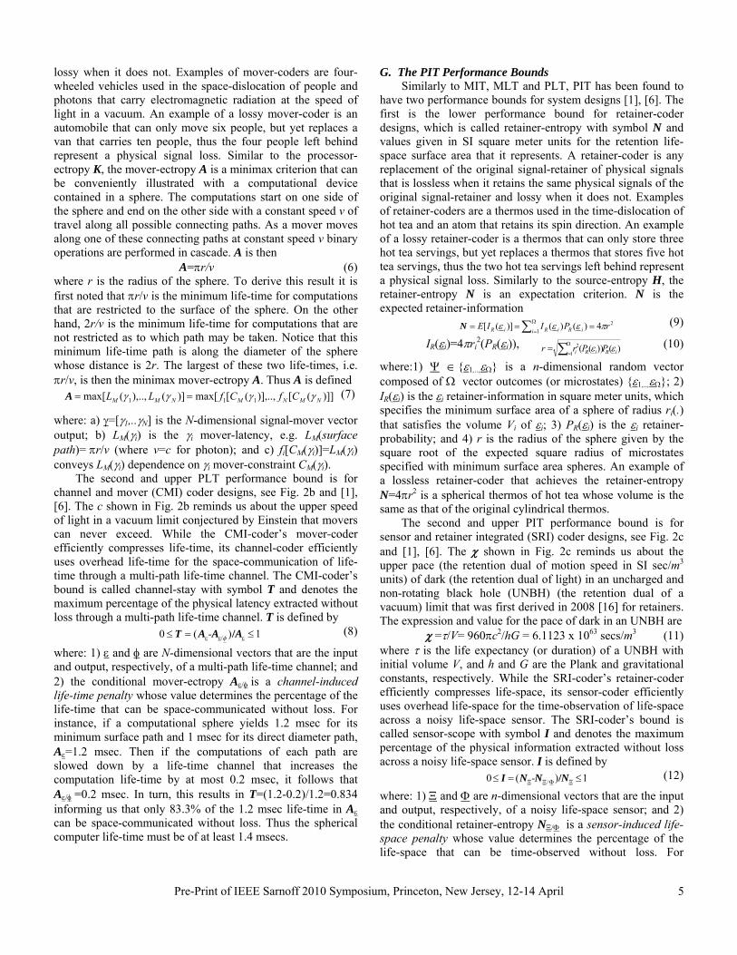
G. The PIT Performance Bounds Similarly to MIT, MLT and PLT, PIT has been found to

have two performance bounds for system designs [1], [6]. The first is the lower performance bound for retainer-coder designs, which is called retainer-entropy with symbol N and values given in SI square meter units for the retention life-space surface area that it represents. A retainer-coder is any replacement of the original signal-retainer of physical signals that is lossless when it retains the same physical signals of the original signal-retainer and lossy when it does not. Examples of retainer-coders are a thermos used in the time-dislocation of hot tea and an atom that retains its spin direction. An example of a lossy retainer-coder is a thermos that can only store three hot tea servings, but yet replaces a thermos that stores five hot tea servings, thus the two hot tea servings left behind represent a physical signal loss. Similarly to the source-entropy H, the retainer-entropy N is an expectation criterion. N is the expected retainer-information

21

4)()()]([ rPIIEi iRiRiR πεεε === ∑Ω

=N (9)

IR(εi)=4πri2(PR(εi)), ∑Ω

==

1 2 )())((

i iRiRi PPrr εε (10)

where:1) Ψ ∈{ε1,..,εΩ} is a n-dimensional random vector composed of Ω vector outcomes (or microstates) {ε1,..,εΩ}; 2) IR(εi) is the εi retainer-information in square meter units, which specifies the minimum surface area of a sphere of radius ri(.) that satisfies the volume Vi of εi; 3) PR(εi) is the εi retainer-probability; and 4) r is the radius of the sphere given by the square root of the expected square radius of microstates specified with minimum surface area spheres. An example of a lossless retainer-coder that achieves the retainer-entropy N=4πr2 is a spherical thermos of hot tea whose volume is the same as that of the original cylindrical thermos.

The second and upper PIT performance bound is for sensor and retainer integrated (SRI) coder designs, see Fig. 2c and [1], [6]. The χ shown in Fig. 2c reminds us about the upper pace (the retention dual of motion speed in SI sec/m3 units) of dark (the retention dual of light) in an uncharged and non-rotating black hole (UNBH) (the retention dual of a vacuum) limit that was first derived in 2008 [16] for retainers. The expression and value for the pace of dark in an UNBH are

χ =τ/V= 960πc2/hG = 6.1123 x 1063 secs/m3 (11) where τ is the life expectancy (or duration) of a UNBH with initial volume V, and h and G are the Plank and gravitational constants, respectively. While the SRI-coder’s retainer-coder efficiently compresses life-space, its sensor-coder efficiently uses overhead life-space for the time-observation of life-space across a noisy life-space sensor. The SRI-coder’s bound is called sensor-scope with symbol I and denotes the maximum percentage of the physical information extracted without loss across a noisy life-space sensor. I is defined by

1)(0 / ≤=≤ ΞΦΞΞ NNNI /- (12)

where: 1) Ξ and Φ are n-dimensional vectors that are the input and output, respectively, of a noisy life-space sensor; and 2) the conditional retainer-entropy NΞ/Φ is a sensor-induced life-space penalty whose value determines the percentage of the life-space that can be time-observed without loss. For


5

instance, if a cylindrical thermos for hot tea with a surface area of 168π cm2 has a retainer-entropy of NΞ=144π cm2, this retainer-entropy can be implemented with a spherical thermos with a 6 cm radius that has the same volume as the original cylindrical thermos. However, if the hot tea is time-observed with a noisy life-space sensor consisting of random people that require the drinking of the hot tea from a thermos cup with a 166π cm2 surface space, the sensor-induced life-space penalty will be of 22π cm2, i.e. NΞ/Φ=22π cm2. In turn, this results in I=(144-22)/144=0.847 informing us that only 84.7% of the 144π cm2 life-space of NΞ can be time-observed without loss. Thus the hot tea life-space must be of at least 166π cm2.

III. THE BRIDGES OF STATISTICAL PHYSICS In this section it is shown that statistical physics, of which

thermodynamics is a special case, offers a natural link between the four LIT quadrants. First a simple relation is noted between the Boltzmann thermodynamics-entropy S and the Shannon source-entropy H [3], i.e.,

HS k 2ln= (13) where S and k, the Boltzmann constant, are given in SI joules per kelvin units and H indicates the expected source-information in bits of the microstates (1). Moreover, when the microstates are equally likely H attains the maximum value of H=log2Ω and S=klnΩ as expected. The thermodynamics-entropy of an uncharged nonrotating black hole (UNBH) has been investigated by Hawking and others [3]-[4], the author inclusive starting in 2008 [16]. The UNBH’s thermodynamics-entropy can be expressed as follows

BitEHEHEH NNHS / 2920ln1/ 2ln/2 2ln/ 3 ==== AchGAck χπ (14) where: 1) EH signifies the ‘event horizon’ where a black-hole meets a vacuum and photon pairs are spontaneously created with one photon emerging inside the vacuum and the other emerging inside the black-hole. While the photon inside the vacuum increases the positive energy of the vacuum, the photon inside the black-hole decreases the positive energy of the black-hole; 2) A is the surface area of the spherical UNBH; 3) SEH, HEH and NEH are the thermodynamics-entropy, source-entropy and retainer-entropy of the UNBH, respectively, with

( )222 /244 cGMrA EHππ ===EHN (15) and MEH being the UNBH mass; and 4) NBit is defined by

(16) BitN 3 /2ln2 chG π= 222 )/2(44 cGMr BitBit ππ ==

PPBit llr 4757.1 2ln == ππ , 3 2/ chGlP π= (17)

RPRP 1774.12ln2 MMMbit == , GhcM RP216/ π= (18)

and denotes the retainer-entropy of a bit that is given by the surface area of a sphere where ½ of its circumference πrBit (rBit is the radius of the sphere) is larger than the Plank length lP as seen from (17) and expected by theory [3]. Moreover, a bit has a mass MBit (or energy for photons) with escape speed close to c (c for photons) exceeding the reduced Plank mass MRP (18).

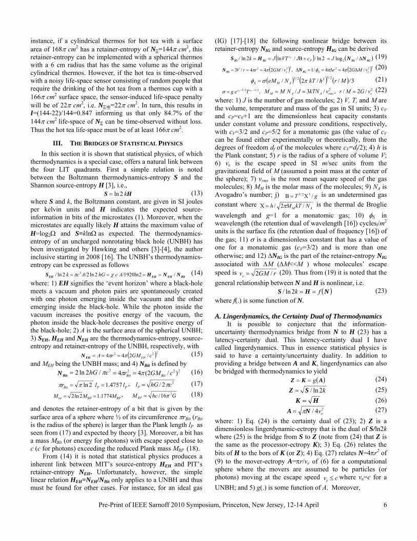
From (14) it is noted that statistical physics produces a inherent link between MIT’s source-entropy HEH and PIT’s retainer-entropy NEH. Unfortunately, however, the simple linear relation HEH=NEH/NBit only applies to a UNBH and thus must be found for other cases. For instance, for an ideal gas

(IG) [17]-[18] the following nonlinear bridge between its retainer-entropy NIG and source-entropy HIG can be derived

( ) ( )IGIGIGIG NNHS Δ=+Β== /log 2ln//ln2ln 2JcJVTJk/ PcV (19)

( ) ,/244/3 222evGMrrV ππ ===IGN ( )222 /244/1 eS vMGr Δ=Δ==Δ ππφIGN (20)

(21) ( ) ( ) ( ) 3// 2/ 2/322/5 /MrhkTNeM AMS πσφ =

(22) where: 1) J is the number of gas molecules; 2) V, T, and M are the volume, temperature and mass of the gas in SI units; 3) c

, 2/32/5 −−= VP cc Tegσ ,/3/ 2rmsAAM vkTNJNMM == 2/2/ evGMr =

V and cP=cV+1 are the dimensionless heat capacity constants under constant volume and pressure conditions, respectively, with cV=3/2 and cP=5/2 for a monatomic gas (the value of cV can be found either experimentally or theoretically, from the degrees of freedom df of the molecules where cV=df/2); 4) h is the Plank constant; 5) r is the radius of a sphere of volume V; 6) ve is the escape speed in SI m/sec units from the gravitational field of M (assumed a point mass at the center of the sphere); 7) vrms is the root mean square speed of the gas molecules; 8) MM is the molar mass of the molecules; 9) NA is Avogadro’s number; j) is an undetermined gas constant where

gT /32/3 Χ=Β

AM NkTMh /2/ π=Χ is the thermal de Broglie wavelength and g=1 for a monatomic gas; 10) φS in weavelength (the retention dual of wavelength [16]) cyclesl/m2 units is the surface fix (the retention dual of frequency [16]) of the gas; 11) σ is a dimensionless constant that has a value of one for a monatomic gas (cV=3/2) and is more than one otherwise; and 12) ΔNIG is the part of the retainer-entropy NIG associated with ΔM (ΔM<<M ) whose molecules’ escape speed is rGMve /2= (20). Thus from (19) it is noted that the general relationship between N and H is nonlinear, i.e.

(23) ( )NHS fk ==2ln/where f(.) is some function of N. A. Lingerdynamics, the Certainty Dual of Thermodynamics

It is possible to conjecture that the information-uncertainty thermodynamics bridge from N to H (23) has a latency-certainty dual. This latency-certainty dual I have called lingerdynamics. Thus in essence statistical physics is said to have a certainty/uncertainty duality. In addition to providing a bridge between A and K, lingerdynamics can also be bridged with thermodynamics to yield

(24) ( )AKZ g==

k2ln/SZ = (25) HK = (26)

24/ evNA π= (27) where: 1) Eq. (24) is the certainty dual of (23); 2) Z is a dimensionless lingerdynamic-ectropy that is the dual of S/ln2k where (25) is the bridge from S to Z (note from (24) that Z is the same as the processor-ectropy K); 3) Eq. (26) relates the bits of H to the bors of K (or Z); 4) Eq. (27) relates N=4πr2 of (9) to the mover-ectropy A=πr/ve of (6) for a computational sphere where the movers are assumed to be particles (or photons) moving at the escape speed where vcve ≤ e=c for a UNBH; and 5) g(.) is some function of A. Moreover,


6

24/ cNA BitBor π= (28)

relates ABor of the NBit’s sphere to NBit to yield the bor ectropy ,4757.1 2ln/ PP TTcrA BitBor === ππ (29) clT P / P =

which is found to be larger than the Plank time TP as expected by theory. Similarly the relationship

24/ eIGIG vNA Δ=Δ π (30)

relates ΔAIG of the ΔNIG’s sphere to ΔNIG. Using the above bridges one obtains for a UNBH

SEH/ln2k = HEH = NEH/NBit = (AEH/ABor)2 = KEH2 = ZEH

2

(31) and for an ideal gas

( ) ( ) 22222 /log/log2ln IGIGIGIGIGIGIGIG ZKAAJNNJHk/S ==Δ=Δ== (32)

The defining expressions for the variables of (31) and (32) given earlier can also be expressed in terms of the physical retention duals of motion variables [16] as well as the lingerdynamics dual for temperature called lingerature. When this is done the following expressions result:

NBit = 4 ln2 lP2= 1920 ln2/cχ (33)

χclP /480= (34) SEH = kNEH /4lP

2 = kcχ NEH /1920 (35)

( ) ( ) ( )223/222 /64/34/24/1 eeSIG ΠOΦvMGN Δ=Δ==Δ πχππφ (36)

τ = 4πr3χ /3 (37) 2 (38) 2243/4 4 4/ cr/acr/GMΦO πχπχτα ===

Gc/ 8143 1210πχΦ = =1.8538 x 10168 Pa.sec4/3/kgR2 (39)

ΔO = ΔMc2/χ (40) cvcrMGOΠ ee /// 2/ 6 3/1 χχτΦ === (41)

( ) ( ) ( ) 3/4/3/ 2/ 3/13 462/322/52 /OchLNceO AMS τπχχπχσφ &&&= (42)

χ/2cMO MM = (43) χ kTL =&&& (44)

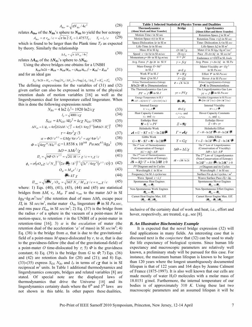
cvcMNkTONLΠ rmsMAMArms /// 3/3 χχ === &&& (45) where: 1) Eqs. (40), (41), (43), (44) and (45) are statistical bridges from ΔM, ve, MM, T and vrms to the mater ΔO in SI kgR=kg.m5/sec3 (the retention dual of mass ΔM), escape pace Πe in SI sec/m3, molar mater OM, lingerature L&&& in SI Pa.sec, and rms pace Πrms in SI sec/m3; 2) Eq. (37) is the bridge from the radius r of a sphere in the vacuum of a point-mass M in motion-space, to retention τ in the UNBH of a point-mater in retention-time [16]; 3) α is the escalation of mater (the retention dual of the acceleration ‘a’ of mass) in SI sec/m6; 4) Eq. (38) is the bridge from a, that is due to the gravitational-field of a point-mass M space-dislocated by r, to α, that is due to the gravidness-fallow (the dual of the gravitational-field) of a point-mater O time-dislocated by τ; 5) Φ is the gravidness constant; 6) Eq. (39) is the bridge from G to Φ; 7) Eqs. (36) and (42) are retention duals for (20) and (21); and 8) Eqs. (33)-(35) express SEH, NBit and lP in terms of cχ that is in SI reciprocal m2 units. In Table 1 additional thermodynamics and lingerdynamics concepts, bridges and related variables [8] are stated. Of special note are the displayed laws of thermodynamics that drive the Universe [18] and its lingerdynamics certainty duals where the 0th and 3th laws are not shown in this table. In other papers these dualities,

Table 1 Selected Statistical Physics Terms and Dualities Thermodynamics

(About Work and Heat Transfer) Bridge Ligerdynamics

(About Effort and Hover Transfer) Motion-Time t in SI sec Retention-Space ξ in SI m3

Motion-Space r(t) in SI m Retention-Time τ (ξ) in SI sec Space-Dislocation Δr in SI m Time- Dislocation Δτ in SI sec

Life-Time Δt in SI sec Life-Space Δξ in SI m3

Mass M in SI kg O=Mc2/χ Mater O in SI kgR=kg.m5/sec3

Speed v =Δr/Δt in SI m/sec Π=vχ/c Pace Π=Δτ/Δξ in SI sec/m3

Momentum p=Mv in SI kg.m/sec pc=υ Endurance υ=OΠ in SI Joule Avg. Force f=Δp/Δt in SI N χγ fv= Avg. Press γ =Δυ/Δξ in SI Pa

Mass-Energy E=Mc2 in SI J

ϖ=E χ

Mater-Viscidity ϖ= Oχ 2

in SI Pa.sec Work W in SI J χWΨ = Effort Ψ in SI Pa.sec Heat Q in SI J χQΛ = Hover Λ in SI Pa.sec

D-less Thermodynamics-Entropy S/ln2k=H is Dimensionless

k2ln/SZ = D-less Lingerdynamics-Ectropy Z=K is Dimensionless

The Thermodynamics Gas Law TJPV &&& = in SI J

χγτ PV=

The Lingerdynamics Gas Law LJ &&& =γτ in SI Pa.sec

Energy-Temperature in SI J ( ) ( ) 2ln/1 HU/US/kkTT ∂∂=∂∂== −&&&

χ TL &&&&&& = Viscidity-Lingerature in SI Pa.sec

( ) ( ) 2ln//2ln// 22 KZ ∂Θ∂=∂Θ∂=L&&&

Internal Energy TJcU V

&&& =

Θ=Uχ Internal Visci ity d

LJcΘ &&& τ=

Heat Capacity Constants cV and cP

cτ=cV and

cγ=cP

Hover Capacity Constants cτ and cγ

Enthalpy Heat PVU +=H

χH=Ξ

Ecthalpy Hover γτ+=ΘΞ

Helmholtz Work TUTU &&&HS 2ln−=−=A

χA=Γ

Helmholtz Effort LΘLΘΓ &&&&&& 22 2ln2ln KZ −=−=

Gibbs Work TTG &&&HS 2ln−=−= HH

χGΥ =

Gibbs Effort LΞLΞΥ &&&&&& 22 2ln2ln KZ −=−=

The 1st Law of Thermodynamics (Conservation of Energy)

ΔU = ΔQ - ΔW

χUΘ Δ=Δ

The 1st Law of Lingerdynamics (Conservation of Viscidity)

ΨΛΘ ΔΔ=Δ - The 2nd Law of Thermodynamics

(Non-Conservation of Entropy) 02ln/ ≥== HS δδδ kTQ

k2ln/SZ δδ =

The 2nd Law of Lingerdynamics (Non-Conservation of Ectropy)

02ln/2ln 22 ≥== KZ δδδ LΛ &&& PV Diagram and its Cycles γτ Diagram and its Cycles

Wavelength λ in SI m Weavelength l in SI sec Frequency f in SI λ cycles/sec Surface Fix φS in l cyclesl / m2

Wave Speed v =λ f Weave Surface Pace ΠS= lφS

Spontaneous Heat ngines ELowHigh TT &&&&&& ⇒

Spontaneous Hove Engines r LowHigh LL &&&&&& ⇒

Non-Spontaneous Work Engines LowHigh TT &&&&&& ⇐

Non-Spontaneous Eff rt Engines oLowHigh LL &&&&&& ⇐

Carnot Heat Engine Max. Eff. ( ) HighLowHigh T/TT &&&&&&&&& −

Carnot Hover Engine Max. Eff. ( ) HighLowHigh L/LL &&&&&&&&& −

inclusive of the certainty dual of work and heat, i.e., effort and hover, respectively, are treated, e.g., see [8]. B. An Illustrative Biochemistry Example

It is expected that the novel bridge expression (32) will find applications in many fields. An interesting case that is discussed next is the conjecture that (32) can be used to study the life expectancy of biological systems. Since human life expectancy and macroscopic parameters are relatively well known, a preliminary study will be pursued for this case. For instance, the maximum human lifespan is known to be longer than 120 years where the longest unambiguously documented lifespan is that of 122 years and 164 days by Jeanne Calment of France (1875-1997). It is also well known that our cells are made mostly of water H2O molecules with a molar mass of 18.0151 g/mol. Furthermore, the internal temperature of our bodies is of approximately 310 K. Using these last two macroscopic parameters and an assumed lifespan it will be


7

shown that (32) predicts a daily caloric intake that correlates well with the expected results.

The development begins by using Clausius’ definition of thermodynamics-entropy to model the daily digestion of food of mass ΔM with the expression

ΔSDig=ΔQ/TDig=C1C2ΔM/TDig in SI J/K units (46) where ΔQ denotes the heat energy in J units of the digested food, TDig is the temperature of digestion, C1=4.2 J/cal and C2=5,000 kcal/kg. On the other hand, it is assumed that a matching or similar amount of mass ΔM is exhaled daily by the human body in the form of a gas. Linked to this exhale that maintains the body mass M and volume V unaltered from day to day, is the Boltzmann thermodynamic-entropy ΔSExh = Sf – Si where Si is the entropy when the day begins and Sf >Si is when it ends. From (32) it is noted that ΔSExh is given by ( ) ( )

IGIG,iIG,fIGIG,iiIGIG,fiifExh kJJJk NNNNNNNSSS ==Δ−ΔΔ+=−=Δ /ln/ln)(

( ))3//(/3/ln ΠNrNrVNNJk IGΔ=Δ=ΔΔ= IGIGIG (47) τ

( )222 /24 4 eIG vGMrN ππ ==

)

)

(48)

( 222 /244/1 eSIG vMGrN Δ=Δ==Δ ππφ (49)

( ) ( ) ( ) ,3// 2/ 2/322/5 /MrhkTNeM ExhAMS πσφ = 2/32/5 −−= VExh

P cc Tegσ (50) 2/3/ / rmsAM vkTJMNM == , (51) 2/2/ evGMr =

1 and 2/ +== VPfV ccdc (52)

V =τ /Π = 4πr3/3 = M/1000 (53) where: 1) τ and Π in (47) and (53) denote a lifespan in secs and retention pace in sec/m3, respectively; 2) the term rΔNIGΠ/3 in (47) corresponds to the M time-dislocation, or weavelength l=rΔNIGΠ/3=86,400 seconds for a single day; 3) J signifies the number of H2O molecules that make up M; 4) ΔJ denotes the number of unknown particles forming ΔM; 5) Eq. (53) assumes that the human mass density is that of liquid water, thus, for instance, if M=70 kg (154.3 lbs) then V=0.07 m3 and r = 0.2557 m; and 6) TExh is the exhale temperature. When (46) and (47) are equated it follows that

(( )2/400,86//ln/000,000'21 MMNNJkTM IGIGDig Δ==ΔΔ=Δ τ . (54) Eqs. (47)-(54) can then be solved under different assumptions, e.g. when M=70 kg, TDig=TExh= 310 K, df=16.1 for H2O at 310 K and τ=130 years (or 4.0997 Gsec) it is found that ΔM = 0.3214 kg for a daily caloric intake of C2ΔM=1,607 kcal (other results derived from (54) are C2ΔM=1,827 kcal if τ=100 yrs, C2ΔM=2,000 kcal if τ=83.4 yrs, etc.). The remaining values for τ=130 years are: 1) σ=1.6672; 2) V=0.07 m3; 3) r=0.2557 m; 4) NIG is 0.8412 m2; 5) ΔNIG =1.7311 x 10-5 m2; 6) J=2.34 x 1027 H2O molecules; 7) ΔJ=1.4643 x 1026 particles with an average molar mass of 1.3216 g/mol for ΔM (e.g. this molar mass is satisfied by 0.1736ΔM of carbon dioxide CO2, 0.0714ΔM of water H2O and 0.755ΔM of hydrogen H atoms); 8) a particle escape speed of ve=19.118 mm/sec; 9) a particle kinetic rms speed of vrms=655.1496 m/sec; 10) a retention pace of Π=58.567 Gsec/m3; 11) a surface fix of φS=57.768 kcyclesl/m2; and 12) a surface pace of ΠS =φSl=4.9911 Gsec/m2. Finally, it should be noted that the previous preliminary study can be readily extended via a multi-species version of (32) to more elaborate molecular models for M.

IV. CONCLUSIONS This paper reviewed the mathematical-physical theory of

communication-observation that is part of latency-information theory or LIT. LIT is expressed in a revolution whose problems fall into two mathematical-intelligence quadrants and two physical-life ones. Using a structural-physical certainty/uncertainty duality conjecture from controls, LIT exhibits design methodologies inherited in each case from classical mathematical information theory or MIT. The efficiency system design philosophy of LIT was illustrated with controls, adaptive radar, physics and biochemistry examples. Moreover, thermodynamics was noted to advance uncertainty bridges for LIT’s MIT and PIT that further illuminate physics retention problems such as those of gases. Using LIT’s conjectured structural-physical dualities, statistical physics was also discovered to have a certainty dual for thermodynamics called lingerdynamics that results in a complete LIT quadrants bridge. The paper ends with an illustration of the conjecture that the derived statistical physics bridge can be used to make reasonable predictions of the daily caloric intake of biological systems for an assumed lifespan.

REFERENCES

[1] Feria, E.H., (2009) “Latency-information theory: A novel latency theory revealed as time-dual of information theory”, Proc. of IEEE Signal Processing Society: DSP Workshop and SPE Workshop, Marco Island, FL, Jan. 2009. LIT publications can be retrieved from author’s website. [2] Shannon, C. E., (1948) “A mathematical theory of communication”, Bell System Tech. Journal, vol. 27, pp. 379-423, 623-656, July, Oct., 1948. [3] Lloyd, S., “Ultimate physical limits to computation”, Nature, Aug. 2000. [4] Bekenstein, J.D., (2007) “Information in the Holographic Universe”, pp. 66-73, Scientific American Reports, Spring 2007. [5] Feria, E.H., (1985) “Matched processors for quantized control: A practical parallel processing approach,” International Journal of Controls, Vol. 42, Issue 3, pp. 695-713, Sept. 1985. [6] _____, (2009) "On a nascent mathematical-physical latency-information theory, Part II: The revelation of a guidance theory for intelligence and life system designs", Proc. of SPIE Defense, Security and Sensing 2009, Vol. 7351-30, pp. 1-16, Orl., Fl., April 14, 2009. [7] _____, (2006), “A predictive-transform compression architecture and methodology for KASSPER, ” Final Technical Report, DARPA Grant FA8750-04-1-0047, May 2006. [8] _____, (2010). Three papers:1) LIT’s Control Roots; 2) Power-Centroid Radar’s LIT Roots; 3) Statistical Physics, Proc. of SPIE Defense, Sec. and Sen. 2010., vol. 7708-29,30,31, Orl.. Florida., 5-9 April 2010. [9] Wozencraft, J.M. and Jacobs, I.M., (1965) “Principles of communication engineering,” Waveland Press, Inc. 1965. [10] Bellman, R. (1957), Dynamic programming, Princeton University Press. Dover paperback edition (2003). [11] Feria, E.H.,(1994),“Decomposed predictive-transform estimation”,IEEE Trans. on Signal Proc., Vol. 42, No. 10, pp. 2811-2822, Oct. 1994, [12] Guerci, J.R. and Feria, E.H., (1996), “Application of a least squares predictive-transform modeling methodology to space-time adaptive array processing,” IEEE Trans. On Sig. Proc., pp.1825-1834, July 1996. [13] Feria, E.H., (2009), "On a nascent mathematical- physical latency- information theory, Part I: The revelation of powerful and fast knowledge-unaided power-centroid radar", Proc. of SPIE Defense, Sec. and Sen.. 2009, Vol. 7351-29, pp. 1-18, Orl., Fl., April 14, 2009. [14] Mano, M.M and Ciletti, M.D., Digital Design, Prentice Hall, 2007. [15] Overbye, D., (2009) “7.3 billion years later, Einstein’s theory prevails”, New York Times, October 28, 2009. [16] Feria, E.H., (2008) “Latency-information theory and applications, Part III: On the discovery of the space dual for the laws of motion in physics”, Proc. of SPIE Def. Sec. Sym., v. 6982-38, pp. 1-18, Apr. 2008. [17] Carter, A.H., Classical and Statistical Thermodynamics, Pr.. Hall, 2001. [18] Atkin, P., “Four laws that drive the Universe”, Oxf. Univ. Press, 2007.


8

the mathematical-physical theory of communication-observation

Documents